Abstract

We study tachyon field inflation in the light of the Planck+WMAP+BICEP2+BAO joint data. While the minimally coupled tachyon field inflation is consistent with the Planck2013 data, it is not confirmed by the Planck+WMAP+BICEP2+BAO dataset. However, a nonminimally coupled tachyon field inflation is consistent with this joint dataset.
PACS: 98.80.Bp,  98.80.Cq,  98.80.Es
Key Words: Inflation, Tachyon Field, Observational Data

1 Introduction

Inflation is a successful paradigm to solve the main problems of the standard cosmological models such as the flatness, horizon and relics problems. The simplest inflationary model is described by a scalar field which slowly rolls down its potential [1, 2, 3]. One of the scalar fields which can be responsible for the early time inflation in the history of the universe, is the tachyon field [4, 5, 6, 7] described by the Dirac-Born-Infeld (DBI) action. There are a wide range of potentials corresponding to this field. So, we confront with several numbers of inflationary models, which their viability should be specified. If a model is consistent with observational data, it can be considered as a viable inflationary model. The recently released observational data, from Background Imaging of Cosmic Extragalactic Polarization (BICEP2) [8], imposes new constraints on the model’s parameters. In this regard, some models are confirmed by observation and some others are ruled out.

Two important parameters in an inflationary models are tensor-to-scalar ratio and the scalar spectral index, which describe the properties of the cosmological perturbations. The limit on the tensor-to-scalar ratio from the combined WMAP9+eCMB+BAO+H₀ data [9], is $r<0.13$. Also, this combined dataset gives the value of the scalar spectral index as $n_{s}=0.9636\pm 0.0084$. The joint Planck+WMAP9+BAO data [10] imposes the constraint $r<0.11$ on the tensor to scalar ratio and gives $n_{s}=0.9643\pm 0.0059$. Now, the Planck+WMAP+BICEP2+BAO dataset  [8, 11], gives new values of these parameters as $r=0.2096^{+0.0443}_{-0.0608}$ and $n_{s}=0.9653^{+0.0129}_{-0.0146}$. The large values of $r$, reported by BICEP2, shows the large amplitude of gravitational wave modes generated during inflation. Another cosmological perturbation parameter which has attracted much interest is the spectral index of the gravitational wave (the tensor spectral index). The Planck+WMAP+BICEP2+BAO dataset gives $n_{t}=1.5261^{+3.4739}_{-3.5261}$. So, this dataset shows the blue tilt of the tensor spectral index which means that the stress-energy tensor violates the Null Energy Condition, meaning that $(\rho+p)<0$, so this is a challengeable result of BICEP2 data. Also, this result doesn’t satisfy the consistency relation $n_{t}=-r/8$, predicted by the standard inflationary model. But, it is demonstrated in [11] that the spectrum of the primordial gravitational waves have significant effect on the CMB TT spectrum at very large scales. Actually, a large change in the positive $n_{t}$ only induces very small change at small angular power. Since at large scales B-mode power is absent, we can not constrain $n_{t}$ tightly with the current observational data. So, it seems that to obtain a reliable value for the tensor spectral index, it should be checked with future experiments.

Here we investigate the status of the tachyon field inflation in the light of recent observational data. By exploring the tensor-to-scalar ratio, scalar spectral index, its running and tensor spectral index, in the background of Planck+WMAP+BICEP2+BAO data, we find that a minimally coupled tachyon field inflation has severe tension with observation and is disproved by recent data. However, a nonminimally coupled tachyon field with some appropriate potentials is consistent with recent observational data.

2 Minimally Coupled Tachyon Field Inflation

The action of a simple inflationary model with a tachyon field, associated with unstable D-branes, can be written as follows

$$S=\int\sqrt{-g}\Bigg{[}\,\frac{1}{\kappa^{2}}R-V(\theta)\sqrt{1-\partial^{\mu}\theta\partial_{\mu}\theta}\,\Bigg{]}d^{4}x\,,$$ (1)

where $\theta$ is the tachyon field, $V(\theta)$ is its potential and $R$ is the 4-dimensional Ricci scalar. In a FRW background, the action (1) leads to the following Friedmann equation

$$H^{2}=\frac{\kappa^{2}}{3}\,\frac{V(\theta)}{\sqrt{1-\dot{\theta}^{2}}}\,.$$ (2)

By variation of the action (1) with respect to the tachyon field we obtaion the equation of motion of the tachyon field as follows

$$\frac{\ddot{\theta}}{1-\dot{\theta}^{2}}+3H\dot{\theta}+\frac{V^{\prime}}{V}=0\,,$$ (3)

where a prime marks a derivative with respect to the tachyon field and a dot refers to derivative with respect to the cosmic time . The energy conservation equation of the model with minimally coupled tachyon field is given by

$$\dot{\rho}_{\theta}+3H(\rho_{\theta}+p_{\theta})=0\,,$$ (4)

where

$$\rho_{\theta}=\frac{V(\theta)}{\sqrt{1-\dot{\theta}^{2}}}\,,$$ (5)

and

$$p_{\theta}=-V(\theta)\sqrt{1-\dot{\theta}^{2}}\,.$$ (6)

For a tachyonic inflationary model the slow roll parameters, which are defined as $\epsilon=-\frac{\dot{H}}{H^{2}}$ and $\eta=-\frac{1}{H}\frac{\ddot{H}}{\dot{H}}$, take the following form [7]

$$\epsilon=\frac{1}{2\kappa^{2}}\frac{V^{\prime 2}}{V^{3}}\,,$$ (7)

and

$$\eta=\frac{1}{\kappa^{2}}\left(\frac{V^{\prime\prime}}{V^{2}}-\frac{1}{2}\frac{V^{\prime 2}}{V^{3}}\right)\,,$$ (8)

Also, the number of e-folds is given by

$$N\simeq-\int_{\theta_{hc}}^{\theta_{f}}\kappa^{2}\frac{V^{2}}{V^{\prime}}d\theta\,.$$ (9)

where $\theta_{hc}$ denotes the value of $\theta$ at the horizon crossing of the scales and $\theta_{f}$ is the value of $\theta$ at the end of inflation.

To test the viability of an inflationary model, studying the spectrum of the perturbations which are produced due to quantum fluctuations of the fields is useful. With a perturbed FRW metric in a longitudinal gauge as [12, 13, 14]

$$ds^{2}=-\big{(}1+2\Phi\big{)}dt^{2}+a^{2}(t)\big{(}1-2\Psi\big{)}\delta_{i\,j}\,dx^{i}dx^{j},$$ (10)

the scalar spectral index, the tensor-to-scalar ratio and the running of the scalar spectral index corresponding to a minimally coupled tachyon model, within the slow-roll approximation ($\dot{\theta}^{2}\ll 1$ and $\ddot{\theta}\ll|3H\dot{\theta}|$), are given as

$$n_{s}-1=-6\epsilon+2\eta,$$ (11)

$$r=\frac{32}{25\pi}\epsilon\,,$$ (12)

and

$$\alpha=\frac{dn_{s}}{d\ln k}$$ (13)

The tensor spectral index in a minimally coupled tachyon model is given by the following expression

$$n_{t}=-2\epsilon\,.$$ (14)

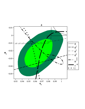
Now, we are going to test this simple model in confrontation with observational data. To this end, we choose several potentials and solve the integral of equation (9). Then we find the value of the scalar field at the horizon crossing and substitute it in equations (11)-(14). Finally we plot the behavior of $r$, $n_{s}$, $\alpha$ and $n_{t}$ in the background of Planck+WMAP+BICEP2+BAO data. The results are shown in figure 1.

Figure 1: Tensor-to-scalar ratio versus the scalar spectral index (a), tensor spectral index versus the scalar spectral index (b), and running of the scalar spectral index versus the scalar spectral index (c), for a model with a minimally coupled tachyon field and in the background of Planck+WMAP+BICEP2+BAO data.

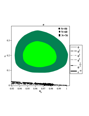
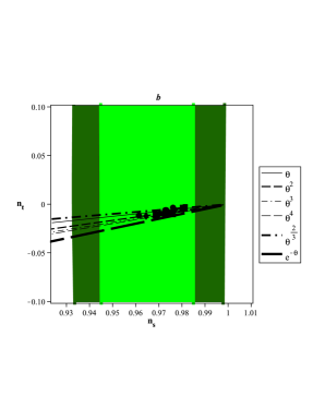
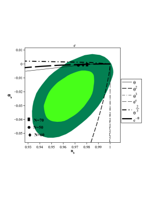
In panel a of figure 1, we have shown the behavior of the tensor-to-scalar ratio versus the scalar spectral index in a model with a minimally coupled tachyon filed and with several potentials. As the figure shows, a tachyon field model with potentials such as a linear potential $V\sim\theta$ [15], a quadratic potential $V\sim\theta^{2}$, a potential as $V\sim\theta^{3}$, a quartic potential $V\sim\theta^{4}$, a potential motivated by axion monodromy, as $V\sim\theta^{\frac{2}{3}}$ [16] and an exponential potential $V\sim e^{-\theta}$ is totally outside the Planck+WMAP+BICEP2+BAO data. We note that a minimally coupled tachyon field inflation with potentials $\theta^{2}$ and $e^{-\theta}$ was supported by the Planck2013 data [7]. Now we see that a minimal tachyon model is ruled out by the Planck+WMAP+BICEP2+BAO joint data. In panel b of figure 1 we have depicted the tensor spectral index versus the scalar spectral index. A minimally coupled tachyon field model predicts a red tilt tensor spectral index, but the value of the tensor spectral index is small. The evolution of the running of the scalar spectral index versus the scalar spectral index is shown in panel c of figure 1. Once again, we see that a minimally coupled tachyon field inflation with mentioned potentials is not supported by this joint dataset. It should be noticed that, with an exponential potential the running of the scalar spectral index is far from the observational data and is not shown in the figure. A minimally coupled tachyon model with an intermediate potential ($V=b\,\theta^{-\beta}\,$ with $\beta=\frac{4l-4}{l-2}$, where $l$ is defined by $a=a_{0}\exp(\vartheta t^{l})$, $0<l<1$) [7] is also quite outside the observational region and is not shown in figure 1.

3 Nonminimally Coupled Tachyon Field

In the presence of a nonminimally coupled tachyon field the action of the model is expressed as follows

$$S=\int\sqrt{-g}\Bigg{[}\frac{1}{\kappa^{2}}R-\frac{1}{2}f(\theta)R-V(\theta)\sqrt{1-\partial^{\mu}\theta\partial_{\mu}\theta}\Bigg{]}d^{4}x\,,$$ (15)

where $f$ is the nonminimal coupling function defined as $f=\xi\theta^{2}$. By using the FRW line element, the Friedmann equation of this model is given by

$$H^{2}=\frac{\kappa^{2}}{3-3\kappa^{2}f}\Bigg{[}\frac{V(\theta)}{\sqrt{1-\dot{\theta}^{2}}}+3f^{\prime}H\dot{\theta}\Bigg{]}\,.$$ (16)

The equation of motion of the tachyon field obtained by varying the action (15) with respect to the field is

$$\frac{\ddot{\theta}}{1-\dot{\theta}^{2}}+3H\dot{\theta}+\frac{V^{\prime}}{V}+\frac{\sqrt{1-\dot{\theta}^{2}}}{2V}f^{\prime}R=0\,.$$ (17)

The presence of the nonminimal coupling changes the energy conservation equation of the model as

$$\dot{\rho}_{\theta}+3H(\rho_{\theta}+p_{\theta})=-3f^{\prime}H^{2}\dot{\theta}\,,$$ (18)

where

$$\rho_{\theta}=\frac{V(\theta)}{\sqrt{1-\dot{\theta}^{2}}}+3f^{\prime}H\dot{\theta}\,,$$ (19)

and

$$p_{\theta}=-V(\theta)\sqrt{1-\dot{\theta}^{2}}-f^{\prime}\ddot{\theta}-2f^{\prime}H\dot{\theta}-2f^{\prime\prime}\dot{\theta}^{2}\,.$$ (20)

The number of e-folds in this setup is given by [7]

$$N\simeq\int_{\theta_{hc}}^{\theta_{f}}\Bigg{(}\frac{3V^{\prime}}{V}\Bigg{)}\Bigg{(}\frac{\kappa^{2}\Big{[}\frac{2VV^{\prime}}{3}-\frac{f^{\prime 2}V^{\prime}R}{3V}-\frac{f^{\prime}V^{\prime 2}}{3V}\Big{]}}{\big{(}1-\kappa^{2}f\big{)}\big{(}-f^{\prime}R-2V^{\prime}\big{)}}\Bigg{)}d\theta\,.$$ (21)

Now we investigate the status of a nonminimally coupled tachyon field inflation in the light of the Planck+WMAP+BICEP2+BAO joint data. In the presence of the nonminimal coupling and with the perturbed FRW metric (10), the scalar spectral index of the model is given by the following expression [7]

$$n_{s}-1=\Bigg{[}\frac{\kappa^{2}\Big{(}f^{\prime}R+2VV^{\prime}\Big{)}}{3H^{2}V\Big{(}1-\kappa^{2}f\Big{)}}-\frac{2V^{\prime}f^{\prime}R-2f^{\prime\prime}R-4V^{\prime\prime}+\frac{4V^{\prime 2}}{V}}{-f^{\prime}R-2V^{\prime}}\Bigg{]}\Bigg{[}\frac{\Big{(}1-\kappa^{2}f\Big{)}\Big{(}-f^{\prime}R-2V^{\prime}\Big{)}}{2V^{2}-f^{\prime 2}R-2f^{\prime}V^{\prime}}\Bigg{]}\,.$$ (22)

The running of the scalar spectral index is obtained by equation (13). The tensor-to-scalar ratio is given by the following expression [7]

$$r\equiv\frac{A_{T}^{2}}{A_{s}^{2}}\simeq\frac{8\pi}{25k^{3}}\Bigg{[}\frac{V^{3}-f^{\prime 2}RV-f^{\prime}V^{\prime}V}{V^{\prime 2}{\cal{C}}}\Bigg{]}\hskip 256.0748pt\\ \times$$

$$\exp\Bigg{[}-2\int\Bigg{(}\frac{\kappa^{2}\Big{(}f^{\prime}R+2VV^{\prime}\Big{)}}{6H^{2}V\Big{(}1-\kappa^{2}f\Big{)}}-\frac{V^{\prime}f^{\prime}R-f^{\prime\prime}R-2V^{\prime\prime}+\frac{2V^{\prime 2}}{V}}{-f^{\prime}R-2V^{\prime}}-\frac{V^{\prime\prime}}{V^{\prime}}+\frac{V^{\prime}}{V}\Bigg{)}d\theta\Bigg{]}$$ (23)

In this setup the tensor spectral index takes the following form

$$n_{t}=\Bigg{(}\frac{-f^{\prime}R-2V^{\prime}}{6H^{2}V}\Bigg{)}\Bigg{(}\frac{\kappa^{2}}{9\big{(}1-\kappa^{2}f\big{)}H^{3}}\Bigg{)}\Bigg{(}-\frac{f^{\prime 2}R}{2V}-\frac{f^{\prime}V^{\prime}}{2V}\Bigg{)}$$

$$\times\Bigg{(}V^{\prime}-\frac{f^{\prime}f^{\prime\prime}R}{V}+\frac{f^{\prime 2}RV^{\prime}}{2V^{2}}-\frac{f^{\prime\prime}V^{\prime}}{V}+\frac{f^{\prime}V^{\prime\prime}}{V}+\frac{f^{\prime}V^{\prime 2}}{V^{2}}+3\kappa^{2}H^{2}\Bigg{)}\,.$$ (24)

Similar to the minimally coupled tachyon field case, we consider some potentials, solve the integral of equation (21) and by using the equations (13) and (22)-(24), we study the behavior of $r$, $n_{s}$, $\alpha_{s}$ and $n_{t}$ in the background of Planck+WMAP+BICEP2+BAO data. The results are shown in the following figures. In figure 2 we have plotted the behavior of the tensor-to-scalar ratio versus the scalar spectral index with several potentials and in the background of Planck+WMAP+BICEP2+BAO data. Figure 3 shows the behavior of the tensor spectral index versus the scalar spectral index with the same potentials. In figure 4 we see the behavior of the running of the scalar spectral index versus the scalar spectral index with the same potentials and in the background of the mentioned dataset. Our numerical analysis shows that a nonminimally coupled tachyon field inflation is observationally viable for some sorts of potential and in some specific ranges of the nonminimal coupling parameter.

Figure 2: Tensor-to-scalar ratio versus the scalar spectral index for a model with a nonminimally coupled tachyon field and in the background of Planck+WMAP+BICEP2+BAO joint data. The panels have been plotted for $N=50$ (a) and $N=60$ (b). Note that, parameter $I$ in the figure refers to Intermediate Potential.

Figure 3: The tensor spectral index versus the scalar spectral index for a model with a nonminimally coupled tachyon field and in the background of Planck+WMAP+BICEP2+BAO joint data. The panels have been plotted for $N=50$ (a) and $N=60$ (b).

Figure 4: The running of the scalar spectral index versus the scalar spectral index for a model with a nonminimally coupled tachyon field and in the background of Planck+WMAP+BICEP2+BAO joint data. The panels have been plotted for $N=50$ (a) and $N=60$ (b).

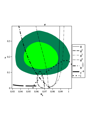
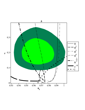
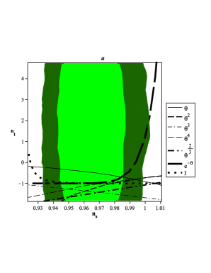
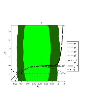
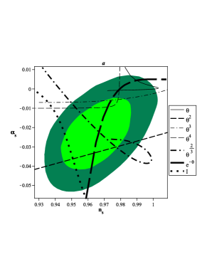
With a linear potential, the nonminimally coupled tachyonic model is consistent with Planck+ WMAP+BICEP2+BAO data if $0.012<\xi<0.078$ (for $N=50$) and $0.0135\leq\xi\leq 0.0794$ (for $N=60$). A nonminimally coupled tachyonic model with a quadratic potential is consistent with recent observational data if $0.081<\xi<0.0883$ (for $N=50$) and $0.0853\leq\xi\leq 0.087$ (for $N=60$). With $V\sim\theta^{3}$, a nonminimally coupled tachyonic model is cosmologically viable if $0.0133<\xi<0.063$ (for $N=50$) and $0.0141\leq\xi\leq 0.0667$ (if $N=60$). With a quartic potential, the Planck+WMAP+BICEP2+BAO data imposes the constraint $0.0101<\xi<0.11$ (for $N=50$) and $0.0106<\xi<0.124$ (for $N=60$) on the model. A nonminimally coupled tachyon model with a potential as $V\sim\theta^{\frac{2}{3}}$ is observationally viable if $0.0122<\xi<0.093$ (for $N=50$) and $0.0130\leq\xi\leq 0.0941$ (for $N=60$). Another potential which we consider here, is an intermediate potential. This potential with a nonminimally coupled tachyon field can be obtained as

$$V=3l^{2}\vartheta^{2}\left({\frac{b}{{\theta}^{2}}}\right)^{\beta}\left(1-{\kappa}^{2}\xi\theta^{2}\right)\kappa^{-2}-{\frac{\kappa^{2}\xi^{2}{\theta}^{2+2\beta}}{1-{\kappa}^{2}\xi\theta^{2}}}\hskip 2.84544pt\\ +\xi\theta\vartheta l{b}^{\beta}\sqrt{{\frac{\kappa^{4}\xi^{2}\theta^{2+2\beta}}{\vartheta^{2}{l}^{2}{b}^{\beta}\left(1-{\kappa}^{2}\xi\theta^{2}\right)^{2}}}+6{\frac{l-1}{\vartheta l}}}\,,$$

where by definition

$$b=\frac{3\left(-2+f\right)^{2}\vartheta l}{8\left(1-l\right)}\,,$$ (25)

and

$$\beta=\frac{2l-2}{-2+l}\,.$$ (26)

With an intermediate potential, there are two constrains on the model; constrains on $\xi$ and $l$. A nonminimally coupled intermediate tachyon field inflation is observationally viable in some ranges of $\xi$ (as shown in the table 1), if $l>0.903$. The constraints on the nonminimal coupling parameter are summarized in table 1. There are two points that should be noticed here. Firstly, with an exponential potential, a nonminimally coupled tachyon field model is still unconfirmed by the Planck+WMAP+BICEP2+BAO data. Secondly, as figure 3 shows, a nonminimally coupled tachyon model with potentials $\theta$, $\theta^{2}$, $\theta^{3}$, $\theta^{4}$, $\theta^{\frac{2}{3}}$ and also the intermediate potential predicts a red tilt of the tensor spectral index. Only with an exponential potential the nonminimally coupled tachyonic model predicts a blue tilt of the tensor spectral index for $\xi<0.071$.

In summary, a minimally coupled tachyon field inflation is not supported by the joint data of Planck+WMAP+BICEP2+BAO since these models predict small values of the tensor-to-scalar ratio in comparison with the recent data. However, the corresponding nonminimal model with potentials $\theta$, $\theta^{2}$, $\theta^{3}$, $\theta^{4}$, $\theta^{\frac{2}{3}}$ and also the intermediate potential is supported well by the mentioned joint dataset. Our numerical analysis sets the constraint $0.0101<\xi<0.124$ on the nonminimal coupling parameter.

Table 1: The ranges of $\xi$ for which a nonminimally coupled tachyon inflation is consistent with the Planck+WMAP+BICEP2+BAO joint data.

$V$		$N=50$		$N=60$
$\theta$		$0.012<\xi<0.078$		$0.0135\leq\xi\leq 0.0794$
$\theta^{2}$		$0.081<\xi<0.0883$		$0.0853\leq\xi\leq 0.087$
$\theta^{3}$		$0.0133<\xi<0.063$		$0.0141\leq\xi\leq 0.0667$
$\theta^{4}$		$0.0101<\xi<0.11$		$0.0106<\xi<0.124$
$\theta^{\frac{2}{3}}$		$0.0122<\xi<0.093$		$0.0130\leq\xi\leq 0.0941$
$e^{-\theta}$		—		—
$I$		$0.041<\xi<0.093$		$0.046\leq\xi\leq 0.084$

References

- [1] A. Guth, Phys. Rev. D, 23, 347 (1981).
- [2] A. D. Linde, Phys. Lett. B, 108, 389 (1982)
- [3] D. H. Lyth and A. R. Liddle, The Primordial Density Perturbation (Cambridge University Press, 2009).
- [4] A. Sen, JHEP, 9910, 008 (1999).
- [5] A. Sen, JHEP, 0207, 065 (2002).
- [6] A. Feinstein, Phys. Rev. D 66, 063511 (2002).
- [7] K. Nozari and N. Rashidi, Phys. Rev. D, 88, 023519 (2013).
- [8] P. A. R. Ade et al. [arXiv:1403.3985 [astro-ph.CO]].
- [9] G. Hinshaw et al., ApJS., 208, 19H.
- [10] P. A. R. Ade et al., [arXiv:1303.5082].
- [11] F. Wu et al. [arXiv:1403.6462 [astro-ph.CO]].
- [12] J. Bardeen, Phys. Rev. D, 22, 1882 (1980).
- [13] V. F. Mukhanov, H. A. Feldman and R. H. Brandenberger, Phys. Rept., 215, 203 (1992).
- [14] E. Bertschinger, [arXiv:astro-ph/9503125], (1995).
- [15] L. Mc Allister, E. Silverstein and A. Westphal, Phys. Rev., D 82, 046003 (2010).
- [16] E. Silverstein and A. Westphal, Phys. Rev., D 78 106003, (2008)