The clustering of galaxies in the SDSS-III Baryon Oscillation Spectroscopic Survey: Baryon Acoustic Oscillations in the Data Release 10 and 11 Galaxy Samples
Abstract
We present a one per cent measurement of the cosmic distance scale from the detections of the baryon acoustic oscillations in the clustering of galaxies from the Baryon Oscillation Spectroscopic Survey (BOSS), which is part of the Sloan Digital Sky Survey III (SDSS-III). Our results come from the Data Release 11 (DR11) sample, containing nearly one million galaxies and covering approximately square degrees and the redshift range . We also compare these results with those from the publicly released DR9 and DR10 samples. Assuming a concordance CDM cosmological model, the DR11 sample covers a volume of 13 Gpc3 and is the largest region of the Universe ever surveyed at this density. We measure the correlation function and power spectrum, including density-field reconstruction of the baryon acoustic oscillation (BAO) feature. The acoustic features are detected at a significance of over in both the correlation function and power spectrum. Fitting for the position of the acoustic features measures the distance relative to the sound horizon at the drag epoch, , which has a value of Mpc in our fiducial cosmology. We find at and at . At 1.0 per cent, this latter measure is the most precise distance constraint ever obtained from a galaxy survey. Separating the clustering along and transverse to the line-of-sight yields measurements at of and . Our measurements of the distance scale are in good agreement with previous BAO measurements and with the predictions from cosmic microwave background data for a spatially flat cold dark matter model with a cosmological constant.
keywords:
cosmology: observations, distance scale, large-scale structure1 Introduction
Measuring the expansion history of the Universe has been one of the key goals of observational cosmology since its founding. To date the best constraints come from measuring the distance-redshift relation over as wide a range of redshifts as possible (Weinberg et al., 2013), and imply that the expansion rate of the Universe has recently transitioned from a deceleration to an acceleration phase (Riess et al., 1998; Perlmutter et al., 1999). While the flat CDM model provides a simple mathematical description of expansion that matches current observations (Planck Collaboration, 2013b), it is physically perplexing given the small vacuum energy density measured, when compared with the high densities that traditionally correspond to new physics (see e.g. Weinberg et al., 2013; Mortonson, Weinberg & White, 2014, for recent reviews). Understanding the physical cause of the accelerating expansion rate remains one of the most interesting problems in modern physics.
One of the most robust methods for measuring the distance-redshift relation is to use the Baryon Acoustic Oscillation (BAO) feature(s) in the clustering of galaxies as a “standard ruler”. The acoustic oscillations arise from the tight coupling of baryons and photons in the early Universe: the propagation of sound waves through this medium gives rise to a characteristic scale in the distribution of perturbations corresponding to the distance travelled by the wave before recombination (Peebles & Yu 1970; Sunyaev & Zel’dovich 1970; Doroshkevich et al. 1978; a description of the physics leading to the features can be found in Eisenstein & Hu 1998 or Appendix A of Meiksin, White & Peacock 1999 and a discussion of the acoustic signal in configuration space can be found in Eisenstein et al. 2007b). This signal is imprinted in the distribution of both the matter and the radiation. The latter are seen as anisotropies in the cosmic microwave background (CMB) radiation while the former are the signal of interest here. The distance that sound waves travel before the coupling between baryons and radiation breaks down, known as the acoustic scale, is quite large, Mpc. The signal therefore relies on simple, linear, well-understood physics that can be well calibrated by CMB anisotropy measurements and is quite insensitive to non-linear or astrophysical processing that typically occurs on much smaller scales. This makes experiments using the BAO signal relatively free of systematic errors.
A number of experiments have used the BAO technique to measure the distance-redshift relationship. The strongest early detections were with galaxies at low-redshift (Cole et al., 2005; Eisenstein et al., 2005; Hutsi, 2006; Tegmark et al., 2006; Percival et al., 2007), though BAO have now also been detected in the distribution of clusters (Veropalumbo et al., 2014), and at higher redshift using the Lyman forest in quasar spectra (Busca et al.,, 2013; Slosar et al., 2013; Kirkby et al., 2013) and cross-correlation betwen quasars and the Lyman forest (Font-Ribera et al., 2013). A review of BAO measurements was provided in Anderson et al. (2012), which described recent experiments (e.g. the 6dFGRS, WiggleZ and SDSS; Beutler et al., 2011; Blake et al., 2011; Padmanabhan et al., 2012), and presented the first set of analyses of the galaxies in Data Release 9 of the Baryon Oscillation Spectroscopic Survey (BOSS Dawson et al., 2012), part of the Sloan Digital Sky Survey III (SDSS III Eisenstein et al., 2011).
In Anderson et al. (2012), we used reconstruction to provide a 1.7 per cent distance measurement from the BOSS DR9 galaxies, the most precise measurement ever obtained from a galaxy survey. This measurement benefitted from a simple reconstruction procedure, that used the phase information within the density field to reconstruct linear behaviour and sharpen the BAO (Eisenstein et al., 2007a). In Anderson et al. (2014) we fitted moments of the anisotropic correlation function measured from the same data, providing distance constraints split into radial and anisotropic directions. We now extend and update the BAO measurements based on the BOSS galaxy samples to the latest dataset from the ongoing BOSS.
This paper concentrates on the DR11 data set, comprised of SDSS-III observations through May 2013, which is scheduled for public release in December 2014 together with the final SDSS-III data release (DR12). The DR10 data set, comprised of observations through June 2012, is already public (Ahn et al., 2013). We provide the DR10 large scale structure samples, including the masks, weights, and random catalogs needed for clustering analyses, through the SDSS-III Science Archive Server. To facilitate community comparisons to our results, in this paper we also present several of our key analyses for the DR10 subset of our data sample.
Five companion papers present extensions to the methodology, testing, and data sets beyond those applied previously to the DR9 data:
- 1.
-
2.
Vargas-Magana et al. (2013) investigates the different possible systematics in the anisotropic fitting methodologies, showing that we achieve unbiased results with fiducial fitting methodology.
-
3.
Manera et al. (2014) describes the production of mock catalogues, used here to determine errors and test our analysis methods.
-
4.
Percival et al. (2014) presents a method to propagate errors in the covariance matrices determined from the mocks through to errors on the final measurements.
-
5.
Tojeiro et al. (2014) presents measurements made at from the low-redshift “LOWZ” BOSS sample of galaxies which we now include in our constraints.
We also have produced a series of companion papers presenting complementary cosmological measurements from the DR10 and DR11 data:
-
1.
Beutler et al. (2013) presents a fit to the CMASS power spectrum monopole and quadrupole, measuring Redshift-Space Distortions (RSD).
-
2.
Samushia et al. (2014) fits the CMASS correlation function monopole and quadrupole, measuring Redshift-Space Distortions (RSD) using a streaming model.
-
3.
Chuang et al. (2013b) fits CMASS correlation function monopole and quadrupole using quasi-linear scales (e.g. above Mpc) to extract single-probe measurements. For the LOWZ sample, they include smaller scales with Finger-of-God modeling.
- 4.
The layout of this paper is as follows. We introduce the data and the catalogue in the next section. The catalogue construction is similar to that described in Anderson et al. (2012) for DR9, and so we focus primarily on the differences and improvements in Section 3. We present the analysis methods for our isotropic and anisotropic measurements in Sections 4 and 5, respectively. We then present the isotropic results in Section 6 and the anisotropic results in Section 7. Our systematic error assessment and final distance measurements are presented in Section 8 and these measurements are placed in a cosmological context in Section 9. We conclude in Section 10.
Throughout the paper we assume a fiducial CDM+GR, flat cosmological model with , , , and , matching that used in Anderson et al. (2012, 2014). Note that this model is different from the current best-fit cosmology; however these parameters allow us to translate angles and redshifts into distances and provide a reference against which we measure distances. The BAO measurement allows us to constrain changes in the distance scale relative to that predicted by this fiducial model.
2 The Data
2.1 SDSS-III BOSS
We use data included in data releases 10 (DR10;Ahn et al. 2013) and 11 (DR11; to be publicly released with the final BOSS data set) of the Sloan Digital Sky Survey (SDSS; York et al., 2000). Together, SDSS I, II (Abazajian et al., 2009), and III (Eisenstein et al., 2011) used a drift-scanning mosaic CCD camera (Gunn et al., 1998) to image over one third of the sky ( square degrees) in five photometric bandpasses (Fukugita et al., 1996; Smith et al., 2002; Doi et al., 2010) to a limiting magnitude of using the dedicated 2.5-m Sloan Telescope (Gunn et al., 2006) located at Apache Point Observatory in New Mexico. The imaging data were processed through a series of pipelines that perform astrometric calibration (Pier et al., 2003), photometric reduction (Lupton et al., 2001), and photometric calibration (Padmanabhan et al., 2008). All of the imaging was re-processed as part of SDSS Data Release 8 (DR8; Aihara et al. 2011).
BOSS is designed to obtain spectra and redshifts for 1.35 million galaxies over a footprint covering square degrees. These galaxies are selected from the SDSS DR8 imaging and are being observed together with quasars and approximately ancillary targets. The targets are assigned to tiles of diameter using a tiling algorithm that is adaptive to the density of targets on the sky (Blanton et al., 2003). Spectra are obtained using the double-armed BOSS spectrographs (Smee et al., 2013). Each observation is performed in a series of -second exposures, integrating until a minimum signal-to-noise ratio is achieved for the faint galaxy targets. This ensures a homogeneous data set with a high redshift completeness of more than per cent over the full survey footprint. Redshifts are extracted from the spectra using the methods described in Bolton et al. (2012). A summary of the survey design appears in Eisenstein et al. (2011), and a full description, including a discussion of the motivation for the targeting criteria, is provided in Dawson et al. (2012).
2.2 Galaxy Catalogues
BOSS selects two classes of galaxies to be targeted for spectroscopy using SDSS DR8 imaging. The ‘LOWZ’ algorithm is designed to select red galaxies at from the SDSS DR8 imaging data via
| (1) | |||
| (2) | |||
| (3) | |||
| (4) |
where here and indicate magnitudes and all magnitudes are corrected for Galactic extinction (via the Schlegel, Finkbeiner & Davis 1998 dust maps), the subscript denotes PSF magnitudes, the subscript denotes ‘model’ magnitudes (Stoughton et al., 2002), the subscript denotes ‘cmodel’ magnitudes (Abazajian et al., 2004), and
| (5) |
and
| (6) |
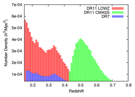
The resulting LOWZ galaxy sample has three times the spatial density of the SDSS-II LRGs, as is shown in Fig. 1, with a similar clustering amplitude to the CMASS sample (Parejko et al., 2013).
We define the effective redshift, , as the mean redshift of a sample weighted by the number of galaxy pairs with separations Mpc. For the LOWZ sample , slightly lower than that of the SDSS-II LRGs as we place a redshift cut to ensure no overlap with the CMASS sample, and hence independent measurements. Further details can be found in Parejko et al. (2013) and Tojeiro et al. (2014). Due to difficulties during the early phases of the project, the sky area of the LOWZ sample lags that of the full survey by approximately , as can be seen in comparison of Tables 1 and 2.
The CMASS sample is designed to be approximately stellar-mass-limited above . These galaxies are selected from the SDSS DR8 imaging via
| (7) | |||
| (8) | |||
| (9) | |||
| (10) | |||
| (11) |
where
| (12) |
and is the -band magnitude within a aperture radius.
For CMASS targets, stars are further separated from galaxies by only keeping objects with
| (13) | |||
| (14) |
unless the target also passes the LOWZ cuts (Eqs. 1-4) listed above.
The CMASS selection yields a sample with a median redshift and a stellar mass that peaks at (Maraston et al., 2013) and a (stellar) velocity dispersion that peaks at (Bolton et al., 2012; Thomas et al., 2013). Most CMASS targets are central galaxies residing in dark matter halos of , but a non-negligible fraction are satellites that live primarily in halos about 10 times more massive (White et al., 2011; Nuza et al., 2013). Further discussion can be found in Tojeiro et al. (2012). Kinematics and emission line properties are described in Thomas et al. (2013).
| DR10 | DR11 | |||||
| Property | NGC | SGC | total | NGC | SGC | total |
| 479,625 | 137,079 | 616,704 | 630,749 | 212,651 | 843,400 | |
| 420,696 | 119,451 | 540,147 | 556,896 | 186,907 | 743,803 | |
| 7,338 | 1,520 | 8,858 | 10,044 | 1,675 | 11,719 | |
| 11,524 | 3,912 | 15,436 | 13,506 | 6,348 | 19,854 | |
| 7,150 | 2,726 | 9,876 | 9,059 | 4,493 | 13,552 | |
| 25,551 | 6,552 | 32,103 | 33,157 | 9,427 | 42,584 | |
| 7,366 | 2,918 | 10,284 | 8,087 | 3,801 | 11,888 | |
| 392,372 | 109,472 | 501,844 | 520,805 | 170,021 | 690,826 | |
| 439,370 | 126,089 | 565,459 | 579,461 | 197,748 | 777,209 | |
| Total area / deg2 | 5,185 | 1,432 | 6,617 | 6,769 | 2,207 | 8,976 |
| Veto area / deg2 | 293 | 58 | 351 | 378 | 100 | 478 |
| Used area / deg2 | 4,892 | 1,375 | 6,267 | 6,391 | 2,107 | 8,498 |
| Effective area / deg2 | 4,817 | 1,345 | 6,161 | 6,308 | 2,069 | 8,377 |
| DR10 | DR11 | |||||
| Property | NGC | SGC | total | NGC | SGC | total |
| 220,241 | 82,952 | 303,193 | 302,679 | 129,124 | 431,803 | |
| 113,624 | 67,844 | 181,468 | 156,569 | 108,800 | 265,369 | |
| 89,989 | 8,959 | 98,948 | 124,533 | 11,639 | 136,172 | |
| 804 | 523 | 1,327 | 944 | 754 | 1,698 | |
| 477 | 278 | 755 | 726 | 497 | 1,223 | |
| 8,199 | 2,928 | 11,127 | 10,818 | 4,162 | 14,980 | |
| 7,148 | 2,420 | 9,568 | 9,089 | 3,272 | 12,361 | |
| 157,869 | 61,036 | 218,905 | 219,336 | 94,444 | 313,780 | |
| 114,905 | 68,645 | 183,550 | 158,239 | 110,051 | 268,290 | |
| Total area / deg2 | 4,205 | 1,430 | 5,635 | 5,793 | 2,205 | 7,998 |
| Veto area / deg2 | 252 | 58 | 309 | 337 | 99 | 436 |
| Used area / deg2 | 3,954 | 1,372 | 5,326 | 5,456 | 2,106 | 7,562 |
| Effective area / deg2 | 3,824 | 1,332 | 5,156 | 5,291 | 2,051 | 7,341 |
Target lists are produced using these algorithms and are then “tiled” to produce lists of galaxies to be observed with a single pointing of the Sloan telescope. Not all targets can be assigned fibers, and not all that are result in a good redshift measurement. In fact, there are three reasons why a targeted galaxy may not obtain a BOSS spectrum:
-
1.
SDSS-II already obtained a good redshift for the object; these are denoted known.
-
2.
A target of different type (e.g., a quasar) is within 62′′; these are denoted missed.
-
3.
another target of the same type is within 62′′; these are denoted cp for “close pair”.
The second and third conditions correspond to hardware constraints on the closest that two fibers can be placed on a plate. In regions where plates overlap, observations of close pairs are achieved. There are two reasons why a spectrum might not result in a good redshift measurement:
-
1.
The spectrum reveals that the object is a star (i.e., it was not properly classified by the imaging data and targeted as a galaxy); denoted star.
-
2.
The pipeline fails to obtain a good redshift determination from the spectrum. These are denoted fail.
The numbers of targets over the sky-region used in our analyses that fall into these categories are given in Table 1 for CMASS and Table 2 for LOWZ. We also report , the total number of galaxies with good BOSS spectra, and , the subset of that pass our redshift cuts. As in Anderson et al. (2012), missed close pairs and redshift failures are accounted for by up-weighting the nearest target of the same target class with a successful spectral identification/redshift (regardless of its category). The LOWZ sample is then cut to and the CMASS sample is cut to to avoid overlap, and to make the samples independent. The regions of sky included for the DR10 and DR11 samples are described in the next section. In order to provide results that use the largest publicly available BOSS data sets, we analyse both the DR10 and DR11 samples throughout this paper.
2.3 Masks
We use the Mangle software (Swanson et al., 2008) to track the areas covered by the BOSS survey and the angular completeness of each distinct region. The mask is constructed of spherical polygons, which form the base unit for the geometrical decomposition of the sky. The angular mask of the survey is formed from the intersection of the imaging boundaries (expressed as a set of polygons) and spectroscopic sectors (areas of the sky covered by a unique set of spectroscopic tiles,see Blanton et al., 2003; Tegmark et al., 2004; Aihara et al., 2011). In each sector, we determine an overall completeness
| (15) |
where is the number of objects in the sector, denotes observed and denotes target. We discard any sectors where . We define the redshift completeness
| (16) |
and discard any sector with . Further details can be found in Anderson et al. (2012), which defined and applied these same two masking choices.
In addition to tracking the outline of the survey region and the position of the spectroscopic plates, we apply several “vetos” in constructing the catalogue. Regions were masked where the imaging was unphotometric, the PSF modelling failed, the imaging reduction pipeline timed out (usually due to too many blended objects in a single field), or the image was identified as having critical problems in any of the 5 photometric bands. We mask the small regions around the centre posts of the plates, where fibres cannot be placed due to physical limitations and also around bright stars in the Tycho catalogue (Høg et al., 2000), with area given by Equation 9 of Anderson et al. (2012). We also place a mask at the locations of objects with higher priority (mostly high- quasars) than galaxies, as a galaxy cannot be observed at a location within the fibre collision radius of these points. In total we masked per cent of the area covered by the set of observed tiles due to our “veto” mask.
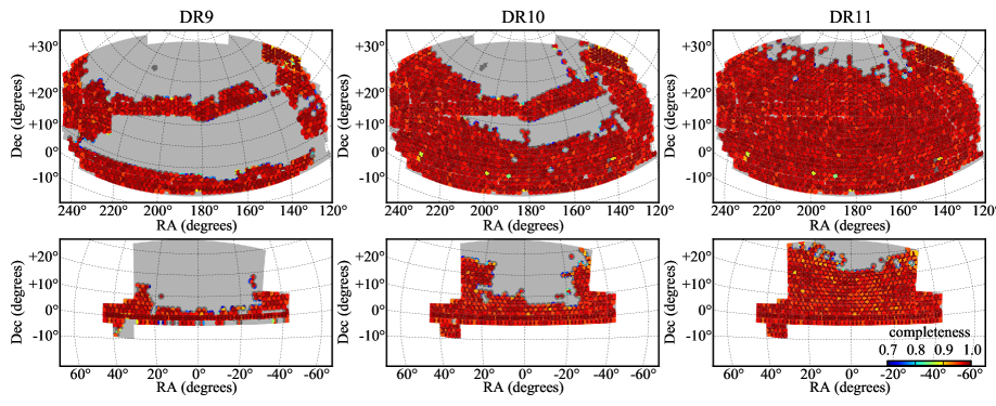
The sky coverage of the LOWZ and CMASS galaxies is shown in Fig. 2 for both the Northern Galactic Cap (NGC) and Southern Galactic Cap (SGC). The ratio of total edge length to total area has decreased significantly with each release, and the effective area has increased from 3,275 deg2 for DR9, to 6,161 deg2, to 8,377 deg2 for the CMASS DR10 and DR11 samples respectively. Tables 1 and 2 list the total footprint area , the area removed by the veto masks , and the total area used . The total effective area is the used area weighted by .
The raw volume enclosed by the survey footprint and redshift cuts is 10 Gpc3 for the DR11 CMASS sample and 3 Gpc3 for the DR11 LOWZ sample, for a total of 13 Gpc3. For these samples, we have also calculated the effective volume, summing over 200 redshift shells
| (17) |
where is the volume of the shell at , and we assume that Mpc3, approximately matching the power spectrum amplitude where the BAO information is strongest. The “holes” in the survey introduced by the veto mask are small, and are better approximated by a reduction in the galaxy density than the volume covered for the large-scale modes of interest. We therefore estimate the galaxy density by dividing the number of galaxies in each shell by the shell volume calculated using area , and the volume of each shell is estimated using area . For DR10, the LOWZ sample then has an effective volume of 1.7 Gpc3, and the CMASS sample 4.4 Gpc3. For DR11, these increase to 2.4 Gpc3 for LOWZ and 6.0 Gpc3 for CMASS.
2.4 Weighting galaxies
To correct for the effects of redshift failures and fiber collisions, each galaxy is given a set of weights. A galaxy is upweighted if its nearest neighbour (of the same target class) had a redshift failure () or a redshift of that neighbour was not obtained because it was in a close pair (). For CMASS, we additionally apply weights to account for the systematic relationships we find between the number density of observed galaxies and stellar density and seeing (weights and , respectively). Each galaxy is thus counted as
| (18) |
where and are equal to 1 for all LOWZ galaxies. In this section, we justify the application of these weights and describe how they are determined.
Ross et al. (2011) created a photometric redshift catalog of the CMASS sample over the full DR8 area, using early BOSS redshifts as a training sample. Using this photometric redshift catalog, Ross et al. (2011) and Ho et al. (2012) found that there exists a significant anti-correlation between the surface number density of CMASS galaxies selected from the SDSS DR8 imaging and stellar density. This relationship was found to impart spurious large-scale clustering in angular distribution of CMASS galaxies.
Ross et al. (2011) and Ho et al. (2012) also found a significant anti-correlation between the number density of CMASS galaxies and seeing of the imaging data. It was found that in areas with poorer seeing the star-galaxy separation algorithm was more restrictive inducing the observed anti-correlation. Using the same catalog, Ho et al. (2012) derived corrections based on measurements of the galaxy-seeing cross-power and applied them to their angular power spectrum measurements, showing that the seeing impacts the measured clustering. Over the DR9 footprint, the impact of the systematic with seeing was found to be insignificant (Ross et al., 2012), as the pattern of seeing over the DR9 area has negligible large-scale power. However, the effect on clustering measured for any given footprint will scale with the pattern of seeing in that particular footprint and any impact on the DR10 and DR11 clustering measurements must be re-tested.
Ross et al. (2012) determined that weights applied to the DR9 CMASS galaxies as a function of stellar density and the magnitude effectively removed any angular and redshift dependence of the CMASS galaxy field on the number density of stars. They found that, while a significant relationship existed between the observed density of CMASS galaxies and seeing, the relationship did not affect the measured clustering. Additional potential systematics such as Galactic extinction, airmass, and sky background were tested and the relationships were consistent with the expected angular variation in galaxy number density. No significant systematic trends were detected in the LOWZ sample.
For the DR10 and DR11 samples, we followed the same procedure as in Ross et al. (2012) to test and model the relation between the density of spectroscopically identified galaxies and stellar density, seeing, Galactic extinction, airmass and sky background. To perform these tests, we made HEALPix (Górski et al., 2005) maps of the DR11 galaxies and compared them to maps of the number of stars with , where is the extinction-corrected -band magnitude, and to maps of the mean values of the potential systematic based on data from the SDSS DR8 Catalog Archive Server (CAS), using various map resolution parameters .
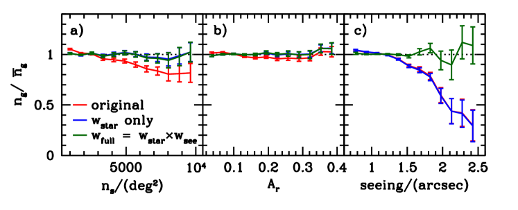
The solid red lines of Fig. 3 show the relationships between the surface number density of galaxies in the CMASS sample, obtained after applying the completeness and close-pair corrections described above, and the stellar density (panel a), Galactic extinction (panel b) and -band seeing (panel c). These lines systematically deviate from , indicating the presence of systematics affecting the galaxy distribution. The error bars in these relations were obtained by applying the same test to the mock catalogues described in Section 3.2. The systematic effect associated with the surface density of stars, , is clearly visible in panel (a), causing a decrease in the number of galaxies of as much as 20 per cent in regions with high stellar density. A weak relation between the observed number of galaxies and the galactic extinction can be seen in panel (b). This is due to the correlation between and and not to an independent systematic. Panel (c) illustrates the strong impact of poor seeing conditions on the observed galaxy number density: an -band seeing of leads to a loss of approximately 50 per-cent of the galaxies. While this effect is dramatic, only 1 per cent of the survey footprint has . The systematic relationship we find between the DR11 CMASS sample and the seeing in the imaging catalog is consistent with relationship found in the DR9 data (Ross et al., 2012).
| DR10 | DR11 | |||
|---|---|---|---|---|
| range | ||||
| 1.015 | -6.3 | 0.998 | 1.1 | |
| 20.3,20.6 | 0.991 | 3.8 | 0.983 | 7.8 |
| 20.6,20.9 | 0.952 | 2.03 | 0.953 | 2.11 |
| 20.9,21.2 | 0.902 | 4.20 | 0.906 | 4.33 |
| 0.853 | 6.42 | 0.870 | 6.06 | |
We use the method to determine the corrective weight for stellar density, , defined in Ross et al. (2012). This method weights galaxies as a function of the local stellar density and the the surface brightness of the galaxy. We use the as a measure of surface brightness and adopt a form for
| (19) |
where and are coefficients to be fit empirically. To construct these weights we divide the CMASS catalogue into five bins of , and fit the coefficients and in each bin so as to give a flat relation between galaxy density and . The stellar density map used for this task is based on a HEALPix grid with , which splits the sky into equal area pixels of 0.21 deg2. This relatively coarse mask is enough to reproduce the large-scale variations of the stellar density. The values of the and coefficients for DR10 and DR11 are given in Table 3. The final weight for a given galaxy is then computed according to the local stellar density by interpolating the binned values of the coefficients and to its observed . The blue lines in Fig. 3 illustrate the effect of applying these weights, which correct for the systematic trend associated with while leaving the relationship with the seeing unchanged, implying there is no significant correlation between the seeing and the stellar density.
Previous analyses of CMASS data (Ross et al. 2011; Ho et al. 2012; Ross et al. 2012) found a systematic dependency with seeing consistent with the one we find for the DR11 CMASS data. In DR9, the relationship was not found to significantly impact the measured clustering and no weight was applied. For DR11, we now find a detectable impact of the relationship with seeing on the measured clustering. We therefore extend the DR9 analyses include a weight, , for the -band seeing, , defined as
| (20) |
which gives a good description of the observed relation. Here the coefficients , and are fitted using the full sample, as opposed to bins of . For this task we use a HEALPix map with (each pixel as a area 0.003 deg2) as high resolution is required to sample the intricate structure of the seeing in the footprint of the survey. The green lines in Fig. 3 show the effect of applying the full weights , which correct for all the observed systematic trends. To avoid applying large weights we set to a constant value for . Introducing is necessary, as we find the pattern of seeing in the SGC has significant angular clustering and thus the systematic induces spurious clustering into SGC measurements. The weights have negligible impact on measurements of the NGC clustering (and, indeed, the DR9 SGC clustering); there is negligible large-scale power in the pattern of the seeing in the NGC data. The best-fit coefficients for the seeing weights we find and apply to the DR10 CMASS data are , and and for DR11 , and . We find no trend in the relationship between galaxy density and seeing as a function of redshift. This implies that weighting based on Eq. 20 removes from the CMASS density field any dependency on seeing in its full 3D space.
3 Analysis changes common to isotropic and anisotropic clustering since DR9
We analyse the BAO feature and fit for distances using the 2-point function in both configuration space (the correlation function, ) and in Fourier space (the power spectrum, ). In Section 4 we present the analysis techniques we use to obtain spherically averaged and and extract isotropic distance scale measurements. In Section 5, we present the analysis techniques we use measure the distance scale along and perpendicular to the line-of-sight using Multipoles and Wedges in configuration space. In this section, we detail the changes common to both the isotropic and anisotropic clustering analysis since DR9. These include changes in: (i) density-field reconstruction, (ii) mock catalogs, and (iii) estimation of errors on these measurements by analyzing mock catalogues.
3.1 Reconstruction
The statistical sensitivity of the BAO measurement is limited by non-linear structure formation. Following Eisenstein et al. (2007a) we apply a procedure to reconstruct the linear density field. This procedure attempts to partially reverse the effects of non-linear growth of structure and large-scale peculiar velocities from the data. This is accomplished using the measured galaxy density field and Lagrangian theory relations between density and displacement. Reconstruction reduces the anisotropy in the clustering, reverses the smoothing of the BAO feature due to second-order effects, and significantly reduces the expected bias in the BAO distance scale that arises from these same second-order effects. Reconstruction thus improves the precision of our BAO scale measurements while simplifying our analyses.
We apply reconstruction to both the LOWZ and CMASS samples. Briefly, we use the galaxy density field, applying an assumed bias for the galaxies, in order to estimate the matter density field and solve for the displacement field. A correction is applied to account for the effect of linear redshift space distortions. Full details of the reconstruction algorithm we apply can be found in Padmanabhan et al. (2012) and Anderson et al. (2012). Compared to Anderson et al. (2012), we have increased the number of points in the random catalogues used both when estimating the displacement field, and when sampling this field to give the shifted field (see Eisenstein et al., 2007a; Padmanabhan et al., 2012; Anderson et al., 2012, for definitions). Internal tests have shown that the results can be biased if the number of points in the random catalogue is too small. Given the large separation between the data in the NGC and SGC, we continue to run reconstruction on these two regions separately.
3.2 Mock catalogs
To create mock galaxy catalogs for LOWZ and CMASS samples we use the the PTHalos methodology described in Manera et al. (2013a) assuming the same fiducial cosmology as the data analysis. The mocks reproduce the monopole and quadrupole correlation functions from the observed galaxies, and are randomly down-sampled to have the same mean as a fitted 10-node spline to the sample . This achieves a smooth redshift distribution for the mean of the mocks. We mask each mock to the area of the observed samples, simulate close-pair completeness (fiber collisions) and randomly downsample to the overall sky completeness based on regions defined by the specific tiling geometry of the data.
To analyse the DR10 and DR11 CMASS samples, 600 mock CMASS galaxy catalogs were used with a slightly updated method as described in Manera et al. (2014). For the LOWZ sample, 1000 mock LOWZ catalogs were created (again assuming the same fiducial cosmology) using a new incarnation of the PTHalos methodology (Manera et al., 2014) that includes a redshift dependent halo occupation distribution. The redshift dependence is fit to the data based jointly on the observed clustering and the observed .
The analysis presented in this paper uses an earlier version of the mocks than the ones that will be publicly released in Manera et al. (2014). The differences are small and include an early estimate of the redshift distribution, a small difference in the way redshifts are assigned to random points, and lower intra-halo peculiar velocities. The mock catalogs are used to test our methodology and estimate covariance matrices. We expect these differences to have negligible statistical and systematic effects, especially when taking the approximate nature of the PTHalos methodology into account. Our systematic error budget is discussed further in Section 9.1.
3.3 Covariance matrices
For each clustering metric we measure on the data, we also measure on the each mock galaxy catalog. We use the distribution of values to estimate the sample covariance matrices that we use in the fitting. We use 600 mock catalogs for CMASS and 1000 for the LOWZ analysis. As the same underlying simulation was used to construct NGC and SGC versions of each mock catalog, we carefully combine a total measurement for each mock by using NGC and SGC measurements from different boxes. The full procedure we adopted is described in detail in Percival et al. (2014), which focuses on understanding the error in the derived covariance matrix. Percival et al. (2014) also includes how we propagate errors in the covariance matrix through to the parameter errors for all results presented in this paper.
4 Measuring isotropic BAO positions
The BAO position in spherically averaged 2-point measurements is fixed by the projection of the sound horizon at the drag epoch, , and provides a measure of
| (21) |
where is the angular diameter distance and is the Hubble parameter. Matching our DR9 analysis (Anderson et al., 2012) and previous work on SDSS-II LRGs (Percival et al., 2010), we assume that the enhanced clustering amplitude along the line-of-sight due to redshift-space distortions does not alter the relative importance of radial and angular modes when calculating spherically averaged statistics. This approximation holds best for our results including reconstruction, which are also our statistically most constraining measures. If we measure the correlation function or power spectrum using a fiducial cosmological model, denoted by a subscript , to convert angles and redshifts into distances, then to an excellent approximation the observed BAO position depends simply on the scale dilation parameter
| (22) |
which measures the relative position of the acoustic peak in the data versus the model, thereby characterising any observed shift. If , the acoustic peak is shifted towards smaller scales, and shifts the observed peak to larger scales. We now outline the methodology we use to measure , tests made using mock catalogues, and how we combine results from , and measurements and from different binning schemes.
4.1 Methodology
We have created separate pipelines to measure the average BAO position in the BOSS data in configuration space using the correlation function, , and in Fourier space using the power spectrum, . The BAO position presents as a single peak in and an oscillation in .
To calculate we use the Landy & Szalay (1993) estimator, summing pair-counts into bins of width (as discussed further in Percival et al., 2014). As a fiducial choice, the smallest bin is centred at , but we will also obtain results for the eight binning choices shifted by increments of . For each binning, we calculate for bin centres in the range (22 bins, for our fiducial choice).
To calculate , we use the Feldman, Kaiser & Peacock (1994) estimator. We use a Fourier grid of size , along each side: this comfortably encloses the survey including both the NGC and SGC components; we use with sufficient zero-padding that aliasing is not a problem which was confirmed by consistency between results from other box sizes. Compared to our DR9 analysis presented in Anderson et al. (2012), we modify our normalisation to properly account for the weights of galaxies introduced to account for nearby close-pair or redshift failures. We calculate in Fourier modes averaged over bin widths of . Percival et al. (2014) find this bin width minimises the combined error when fluctuations in the covariance matrix are also included. Our fiducial choice has the smallest -bin centred at . We will also use the nine additional binning schemes that shift the bin centres by increments of . We calculate for bin centres in the range , giving 35 bins for our fiducial choice. These limits are imposed because the BAO have effectively died out for smaller scales, and larger scales can be sensitive to observational systematics.
We fit the measured, spherically averaged, correlation function and power spectrum separately and then combine results using the mocks to quantify the correlation coefficient between measurements. Our fits use polynomial terms to marginalise over the broad-band shape in either 2-point measurement, while rescaling a model of the damped BAO to fit the data. We use slightly different template BAO models for and fits, as they enter the model functions in different ways.
To produce a template model for the fit, we first compute a linear power spectrum produced by Camb (Lewis et al., 2000). We then split into two components, one oscillatory and the other smooth , that return the Camb derived power spectrum when multiplied together. To perform the split, we fit using the same method that we use to fit to the data, but with a BAO model calculated using the fitting formulae of Eisenstein & Hu (1998). The resulting smooth model is taken to be , and is calculated by dividing by this. This follows the procedure used in Anderson et al. (2012).
The full model fitted to the data power spectrum is then
| (23) |
where
| (24) |
There are therefore six “nuisance” parameters: a multiplicative constant for an unknown large-scale bias , and five polynomial parameters, , , , , and , which marginalise over broad-band effects including redshift-space distortions, scale-dependent bias and any errors made in our assumption of the model cosmology. These effects may bias our measurement of the acoustic scale if not removed.
The damping was treated as a free parameter, with a Gaussian prior with conservative width Mpc centered at the best-fit values recovered from the mocks: for the CMASS sample these are Mpc pre-reconstruction, and Mpc post-reconstruction and for LOWZ they are Mpc pre-reconstruction and Mpc post-reconstruction. This model, which differs from that used to fit the power spectrum in Anderson et al. (2012), is better matched to the now standard model for the correlation function (e.g. Anderson et al., 2012) that we adopt.
To fit to the correlation function, we adopt the template model for the linear correlation function given in Eisenstein et al. (2007b), with damped BAO
| (25) |
where the Gaussian term has been introduced to damp the oscillatory transform kernel at high- to induce better numerical convergence. The exact damping scale used in this term is not important, and we set Mpc, which is significantly below the scales of interest. The power spectrum is given by
| (26) |
where is the same model produced by Camb, and used to create the power spectrum fit template. is a model created using the no-wiggle fitting formulae of Eisenstein & Hu (1998), in which the BAO feature is erased. We refer to this template as the “De-Wiggled” template.
Using this template, our correlation function model is given by
| (27) |
where is a multiplicative constant allowing for an unknown large-scale bias, and the additive polynomial is
| (28) |
where help marginalize over the broadband signal.
Unlike for the power spectrum, we do not allow the damping parameter to vary and instead fix it at the average best-fit value recovered from the mocks: the interplay between and the additive polynomial in our fit to means that the amplitude of the BAO peak has more freedom already.
Apart from the differences in damping correction, the parallel between and fitting methods is clear and follows from the match between Eq. (23) & (26) and between Eq. (24) and the combination of Eqns. (27) & (28). There are three subtle differences: For the power spectrum we only shift the BAO with the parameter , while for we shift the full model. As the nuisance parameters are marginalising over the broadband, this should have no effect. For the correlation function, the nuisance parameters are added to the final model compared to the data ; for the power spectrum, they are added to the smooth model . This slightly changes the meaning of the BAO damping term. We also split the CAMB power spectrum into BAO and smooth components in different ways, utilising the Eisenstein & Hu (1998) functions for the template, whereas for the fit we can applying the same fitting method to the CAMB power spectrum as used to fit the data. The effect of this is expected to be small.
For fits to both the correlation function and power spectrum, we obtain the best-fit value of assuming that and were drawn from multi-variate Gaussian distributions, calculating at intervals of in the range . Our final error on is determined by marginalising over the likelihood surface and then correcting for the error in the covariance matrix as described in Percival et al. (2014).
4.2 Testing on Mock Galaxy Catalogs
We test our and isotropic BAO fitting procedure on each of our CMASS mock galaxy samples, both pre- and post-reconstruction. The results are summarised in Table LABEL:tab:mockbao. Tojeiro et al. (2014) presents similar tests on the LOWZ mock galaxy samples.
| Estimator | /dof | |||
|---|---|---|---|---|
| DR11 | ||||
| Consensus + | 1.0000 | 0.0090 | 0.0088 | |
| combined | 1.0001 | 0.0092 | 0.0089 | |
| combined | 0.9999 | 0.0091 | 0.0090 | |
| post-recon | 1.0001 | 0.0093 | 0.0090 | 28.6/27 |
| post-recon | 0.9997 | 0.0095 | 0.0097 | 17.6/17 |
| pre-recon | 1.0037 | 0.0163 | 0.0151 | 27.7/27 |
| pre-recon | 1.0041 | 0.0157 | 0.0159 | 15.7/17 |
| DR10 | ||||
| post-recon | 1.0006 | 0.0117 | 0.0116 | 28.4/27 |
| post-recon | 1.0014 | 0.0122 | 0.0126 | 17.2/17 |
| pre-recon | 1.0026 | 0.0187 | 0.0184 | 27.7/27 |
| pre-recon | 1.0038 | 0.0188 | 0.0194 | 15.8/17 |
Overall, we find a small, positive bias in the mean recovered values pre-reconstruction, varying between 0.0026 (DR10 ) and 0.0041 (DR11 ). This bias is significantly reduced post-reconstruction, as expected (Eisenstein et al., 2007b; Padmanabhan & White, 2009; Noh, White & Padmanabhan, 2009; Mehta et al., 2011). For the post-reconstruction DR11 samples, given that the uncertainty on one realisation is 0.009, the statistical () uncertainty on is 0.0004. The and results are both consistent with 1 (i.e. unbiased). This result is independent of bin size.
In general, the mean uncertainties recovered from the individual likelihood surfaces are close to the standard deviation in the recovered . All of these values include the appropriate factors to correct for the biases imparted by using a finite number of mocks, determined using the methods described in Percival et al. (2014). The agreement between the recovered uncertainty and the standard deviation suggests that our recovered uncertainties are a fair estimation of the true uncertainty.
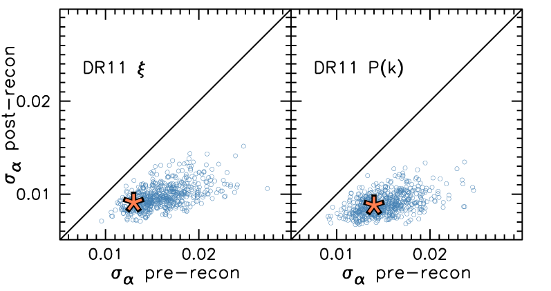
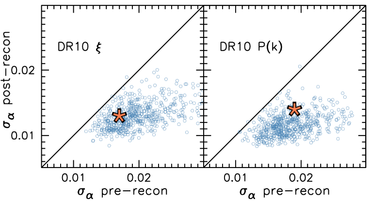
Applying reconstruction to the mock galaxy samples improves the uncertainty in BAO fits substantially. Fig. 4 displays scatter plots of before and after reconstruction for the DR11 (top) and DR10 (bottom) samples for (left) and (right). For DR11 reconstruction reduces the uncertainty in every case. The mean improvement, determined by comparing pre- and post-reconstruction, is more than a factor of 1.5 in every case and is even more for the DR11 results.
In summary, DR11 CMASS post-reconstruction and measurements are expected to yield estimates of the BAO scale, with statistical uncertainties that are less than 1 per cent, obtained from likelihood errors that agree with the standard deviation found in the measurements obtained from the mock samples. Furthermore, post-reconstruction, the systematic errors on the value of measured from the mocks are consistent with zero for both correlation function and power spectrum fits, with an error on the measurement of per cent. Section 8.1 considers possible systematic errors on our measurements in more detail.
4.3 Combining Results from Separate Estimators
We have used and to measure the BAO scale for a number of different binning choices, with different values of bin centres and bin sizes in and respectively. These do not yield perfectly correlated BAO measurements because shot noise varies within each binning choice. Each estimate is un-biased, and we can therefore combine BAO measurements using different binning schemes and different estimators, provided we take the correlation into account, which we will do using the mocks. This results in more precise measurements of the BAO scale.
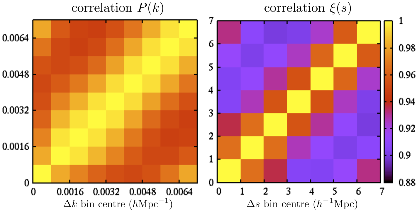
The dispersion in values of that we recover from the mocks for a single choice of bin width but with different bin centres, is greater for than for . There is therefore more to be gained by combining results from offset bins for our analysis of . The correlation matrices for recovered from the eight and the ten bin centres tested (see Section 4.1) are displayed in Fig. 5. For , the correlation is as low as 0.89. The results are more correlated, as all of the correlations are greater than 0.94.
The fact that results using different bin centres are not perfectly correlated implies that an optimised measurement can be made by calculating the weighted mean of across all of the bin centre choices. The process we use is as follows: We find the weighted mean uncertainty, , using the correlation matrix,
| (29) |
We then scale the elements of by to obtain the covariance matrix, , for the measurements at each bin centre. The BAO scale measurement, , and its uncertainty, , obtained combining the results across bin centres are then given by
| (30) |
Applying this to and decreases the uncertainty and standard deviation such that they are nearly identical for and , shown as the “combined” results in Table LABEL:tab:mockbao.
The method we apply to measure the BAO position from has changed from the method applied in Anderson et al. (2012); it is now more similar to the method applied to the measurements (e.g., the smooth polynomials are similar). We combine information across bin centre choices for both fits. This results in BAO measurements that are more correlated between fits to and . We use
| (31) |
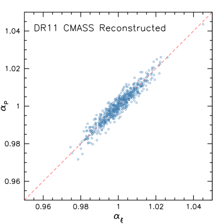
to quantify the correlation between two measures, where in this case represents the standard deviation of sample . For the DR11 CMASS reconstructed mock galaxy samples, we find . Fig. 6 displays a scatter plot illustrating this tight correlation.
In order to combine BAO measurements from and , we take as the mean of the two estimates and its uncertainty as , where is the mean uncertainty of the two estimates. This allows the uncertainty to vary for any given realisation, but assumes that the uncertainty is equal and Gaussian distributed for and . The 0.987 factor is the reduction in uncertainty obtained by averaging two measurements with a 0.95 correlation factor that we identified from the mock measurements.
5 Measuring Anisotropic BAO Positions
Assuming an incorrect cosmology when calculating the galaxy correlation function or power spectrum will differentially shift the BAO feature in both the transverse and line-of-sight directions. These shifts are typically parameterized by and , which are the natural extension of the isotropic scale dilation factor introduced in Section 4. Together, they allow us to measure the angular diameter distance (relative to the sound horizon at the drag epoch ) , and the Hubble parameter via separately through
| (32) |
Another parameterization that exists in the literature decomposes the anisotropic shifts into and an anisotropic warping factor , which can be defined in terms of and as
| (33) |
Note that in the fiducial cosmology, and . In this paper, we concentrate on and , but there are discussions that use and parameterization for the ease of explanation. In particular, we use - and - interchangeably for multipoles as we can convert one to another parameterization easily. Note that the measured through anisotropic clustering is in theory the same as measured using isotropic clustering. However, there can be a small amount of scatter between the two measured s.
We have developed separate pipelines using either multipoles of the correlation function, or top-hat windows in (called wedges Kazin et al., 2012), to estimate and . We now outline the methodology behind each pipeline and present the results of tests on both using mock data.
5.1 Methodology
For the CMASS data we measure the average BAO position in configuration space using moments of the correlation function, , where is the cosine of the angle between a galaxy pair (we use the mid-point of the two galaxy positions in redshift space) and the line-of-sight. We use the CMASS galaxy catalog only and we don’t do an anisotropic Fourier space analysis in this paper (see Beutler et al., 2013, for a complementary analysis). We measure using the Landy & Szalay (1993) estimator, with radial bins of width and angular bins of (see Percival et al., 2014; Vargas-Magana et al., 2013, for the effect of bin-sizes on the measurement). We then project the -dependence to obtain both “multipoles”
| (34) |
and “wedges”,
| (35) |
Throughout we shall denote the Legendre polynomial of order as , since will be reserved for moments of the power spectrum. As wedges and multipoles are alternative projections of , we expect similar constraints from both. We perform both analyses principally as a test for systematic errors.
For both cases we only measure and fit to two projections. For the multipoles we use and 2. In linear theory there is information in the multipole as well, and beyond linear theory there is information in all even multipoles, but we do not include the higher multipoles as the increase in signal-to-noise ratio is small compared to the increase in modeling complexity. Furthermore, after reconstruction, the effect of redshift space distortions is significantly reduced, decreasing the information in further. For the wedges, we choose such that we have a bin which is primarily “radial”, , and a bin which is primarily “transverse”, . This matches the methodology adopted for the anisotropic DR9 BAO measurements presented in Anderson et al. (2014).
We model the moments of the correlation function as the transform of
| (36) |
where
| (37) |
is a streaming model for the Finger-of-God (FoG) effect (Peacock & Dodds, 1994) and is the streaming scale, which we set to . This choice of the streaming scale has been tested in Xu et al. (2012b); Anderson et al. (2014); Vargas-Magana et al. (2013). The term is the linear theory prediction for redshift-space distortions at large scales (Kaiser, 1987). In linear theory , where is the linear growth rate, but we treat as a parameter which we vary in our fits. This allows for modulation of the quadrupole amplitude, as is degenerate with any quadrupole bias. To exclude unphysical values of we a impose a prior. This prior is discussed further in Section 5.2 and its effects tested in Section 7.3. We take to be:
| (38) |
where the term includes some of the non-linearities to second order, and is given by (Goroff et al., 1986; Makino, Sasaki & Suto, 1992; Jain & Bertschinger, 1994):
| (39) |
with given by Eq. (45) of the review of Bernardeau et al. (2002) or the references above. The parameter accounts for the damping of the baryonic acoustic feature by non-linear evolution and for the induced coupling between Fourier modes. We fit to the mocks with these parameters free and use the mean value of the best-fits pre-reconstruction and post-reconstruction. In particular, is fixed to Mpc and is fixed to pre(post)-reconstruction.
The template of Eq. (38) is different from the one used in Anderson et al. (2014) and from the non-linear template used in Section 4. The isotropic fitting in both configuration and Fourier space used the “De-Wiggled” template (Eq. 26), while we use , inspired by renormalized perturbation theory. This template was previously used by Kazin et al. (2013) in the analysis of the CMASS DR9 multipoles and clustering wedges and is described in more detail in Sánchez et al. (2013a).
We then decompose the full 2D power-spectrum into its Legendre moments:
| (40) |
using from Eq. (36), which can then be transformed to configuration space using
| (41) |
where, is the -th spherical Bessel function.
Similar to the isotropic BAO fitting procedure (Section 4), we use polynomial terms to marginalize over the broad-band shape for both multipoles and wedges. The model multipoles, , and projections, , are defined by our template evaluated for the fiducial cosmology. The model fit to the observed multipoles is then
| (42) |
and to the observed wedges is
| (43) |
where Xu et al. (2012b) describe how to include and in the template and Kazin et al. (2013) describe the equivalent methodology for . The parameters are bias factors that rescale the amplitude of the input models, while regulates the amplitude ratio of the two wedges. The polynomial terms
| (44) |
are used to marginalize out broadband (shape) information that contributes to due to, e.g., scale-dependent bias or redshift-space distortions.
In order to find the best-fit values of and , we assume that the correlation function moments are drawn from a multi-variate Gaussian distribution with a covariance matrix derived from our mocks (Manera et al., 2014), corrected as summarized in Section 3.3. We fit to 40 points over the range , including both the monopole and the quadrupole or the two wedges. Since there are 10 parameters in our fitting model, this gives 30 degrees of freedom in the fit.
In our analysis of the wedges, we use a Markov chain Monte Carlo (MCMC) to explore the parameter space
| (45) |
We impose flat priors in all these parameters and obtain our constraints on and by marginalizing over all the remaining parameters.
In our analysis of the multipoles, we explore the parameter space by calculating the likelihood surface over a large grid of and with , and 111We have tested the effect of grid size on and and have verified that finer grids results in no difference to the errors recovered (Vargas-Magana et al., 2013).. Before performing the fit, we normalize the model to the data at and hence . As mentioned previously, we allow to vary in our fits but apply two priors:
-
•
Gaussian prior on centered on , with standard deviation of .
-
•
Gaussian prior on with a standard deviation of 0.2. The central value is set to pre-reconstruction, and zero post-reconstruction (Xu et al., 2012b).
For each grid point, (,), we fit the remaining parameters to minimize the . Assuming the likelihood surface is Gaussian allows us to estimate the uncertainties of and as the standard deviations of the marginalized 1D likelihoods (for more details see Xu et al. 2012b and Vargas-Magana et al. 2013). The deviations are computed by integrating the likelihood surface over and . We do however use an expanded likelihood surface covering a wider range of and as input for measuring cosmological parameters, so the chosen integration intervals do not have any effect on the down-stream cosmological analysis. We test the effect of each of these priors in Section 5.2. We can then easily convert any (,) to (,).
5.2 Testing on Mock Galaxy Catalogues
We test our anisotropic BAO fitting procedure with both multipoles and wedges, pre- and post-reconstruction using mock catalogs. The results are summarized in Table 5. We list the median values of the recovered , , and from all the mock galaxy samples. Pre-reconstruction, we find that there is a small positive bias (0.006) in the median using multipoles and a small negative bias (-0.004) when using wedges. The signs of biases are reversed for , as (again pre-reconstruction) there is a small negative bias (-0.003) for multipoles and a small positive bias (0.001) for wedges. Reconstruction reduces the bias. Post-reconstruction, the largest bias is 0.003 for the median multipole . The others are all . Finally, we note that both the standard deviation of the s and the median of their errors are very consistent. The uncertainties are also significantly larger than the biases on (the bias is at most 11% of the uncertainty on s) for both methods.
Anderson et al. (2014) and Kazin et al. (2013) describe detailed tests applied to the “Wedges” technique. Given the high degree of correlation between wedge and multipole based measurements and fitting methodology of multipoles has changed slightly since Anderson et al. (2014), here we focus on tests based on multipoles.
We tested the robustness of our fits to a number of parameter choices, including the following:
-
•
Changing fitting ranges
-
•
Changing the number of nuisance parameters,
-
•
Changing the priors on and .
The results of these and further tests are extensively detailed in Vargas-Magana et al. (2013). Here we only highlight the specific findings that are pertinent to this analysis (see Table 6). None of the tests resulted in significantly biased values for the best fit parameters or their associated errors. In particular, the best fit values of do not vary by more than per cent for all cases, and most of the best fit values of do not vary by more than per cent. It is particularly interesting to note that the median errors of both and do not change at all for all of the different fitting parameter choices. Note that this is not true if we extend the range of and over which we integrate to make these measurements. By design, the priors act to exclude unphysical models, which otherwise can affect the measured errors. However, the likelihood close to the best-fit solution is not affected by these priors, and hence the best-fit values and errors are not affected.
| Method | ||||||||||||
|---|---|---|---|---|---|---|---|---|---|---|---|---|
| Post-Rec DR11 | ||||||||||||
| Consensus | - | - | - | - | 1.0009 | 0.0252 | 0.0270 | 0.0045 | 0.9984 | 0.0143 | 0.0149 | 0.0018 |
| Multipoles | 1.0002 | 0.0092 | 0.0011 | 0.0122 | 1.0032 | 0.0266 | 0.0248 | 0.0072 | 0.9999 | 0.0149 | 0.0137 | 0.0018 |
| Wedges | 1.0003 | 0.0090 | 0.0005 | 0.0124 | 1.0006 | 0.0264 | 0.0296 | 0.0052 | 0.9993 | 0.0153 | 0.0161 | 0.0026 |
| Pre- Rec DR11 | ||||||||||||
| Multipoles | 0.9995 | 0.0155 | 0.0022 | 0.0189 | 1.0058 | 0.0443 | 0.0384 | 0.0150 | 0.9965 | 0.0210 | 0.0205 | 0.0033 |
| Wedges | 0.9991 | 0.0152 | -0.0011 | 0.0207 | 0.9965 | 0.0475 | 0.0466 | 0.0137 | 1.0007 | 0.0222 | 0.0230 | 0.0086 |
| Model | ||||||||
|---|---|---|---|---|---|---|---|---|
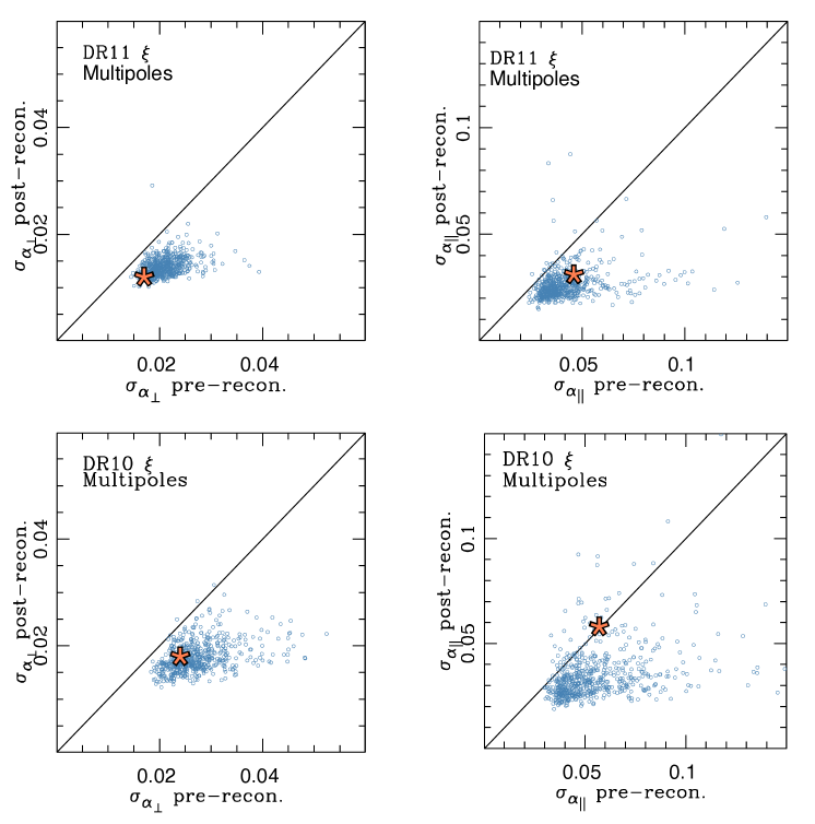
Finally, we further test our Multipoles method by looking at the error on both and for all of our mock galaxy samples (blue points), and compare it to our data in DR10 and DR11 (orange stars). We show in Figure 7 that reconstruction decreases the uncertainty on and in the vast majority of the 600 mock galaxy samples. This is especially true for . The DR10 footprint is less contiguous than the DR11 one and there are thus more outliers in DR10 than in DR11 where reconstruction does not improve the uncertainty. The constraints obtained using the pre- and post-reconstruction wedges show a similar behavior.
5.3 Comparing and Combining Methodologies
Table 5 compares the fitting results of our DR11 mock galaxy catalogs using the multipoles and clustering wedges. There are slight differences in both the median and dispersion between methods in pre-reconstruction, but both are unbiased and give similar errors in both and . For instance, the median and the 68% confidence level of the variation between the two methods, , is while that for is . These are small differences, especially when compared to the standard deviations ( and ) within the mocks, which are on the order of and respectively.

As we can see from Table 5, the fitting results of post-reconstructed mock catalogs from both methods are extremely similar. After reconstruction, the median BAO measurements become even more similar between the two methods and the scatter, relative to the standard deviation, decreases slightly: we find and . The top panels of Fig.8 show scatter plots between the BAO measurements for multipoles and those of wedges, post-reconstruction, determined from the 600 mock samples. The two measurements are clearly correlated.
We find that the multipole results are slightly more precise, on average. We obtain tight constraints on both and . In particular, and pre-reconstruction and post reconstruction, while the median difference in best-fit values are and . As measurements from the two fitting methodologies are clearly correlated, it is not surprising that the obtained precisions on the s are similar.
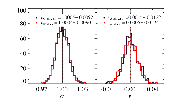
For reasons that will become apparent later in Sec 7, we also look at the differences in fitting results between wedges and multipoles when we measure and , in addition to and . In Figure 9 , we show the histogram of the fitted and from the two different methodologies used in anisotropic clustering. The median values of s are almost identical in the two methodologies with close to zero median shift. The distributions show small median shift of 0.2 and -0.1 per cent which point in different directions for multipoles and wedges approaches respectively. The standard deviations in both and from both methods are also comparable.
In general, the statistics indicate a good agreement between the distributions of the fitted parameters and errors obtained from multipoles and wedges. We do not find any indication that favours one technique over the other. Pre-reconstruction we find differences of 0.2 in the median values of and recovered by the two methods, but post-reconstruction these differences become negligibly small, less than 0.08. We therefore believe that the two methods are equally un-biased. The scatter in the results recovered by the Multipoles and Wedges methods in individual realizations come from shot-noise and differences in methodology, as explored further in Vargas-Magana et al. (2013).
Given that the multipoles and wedges results are both unbiased but are not perfectly correlated, our results are improved by combining the two results. We do this following the procedure adopted in Anderson et al. (2014). Briefly, we take the mean of the log-likelihood surfaces obtained using each method and use this averaged likelihood surface to obtain consensus results. We have applied this procedure to the results from each mock realisation and the statistics are listed as the “consensus” values in Table 5. The standard deviation in both the BAO measurements and their uncertainties have decreased, showing that a small improvement is afforded by combining the two measurements.
6 BAO Measurements from Isotropic Clustering Estimates
6.1 Clustering Estimates
In the previous sections, we detailed our analysis techniques and demonstrated they recover un-biased estimates of the BAO scale. We now apply our results to the BOSS data. We present our isotropic measurements in this section and our anisotropic results in the following section.
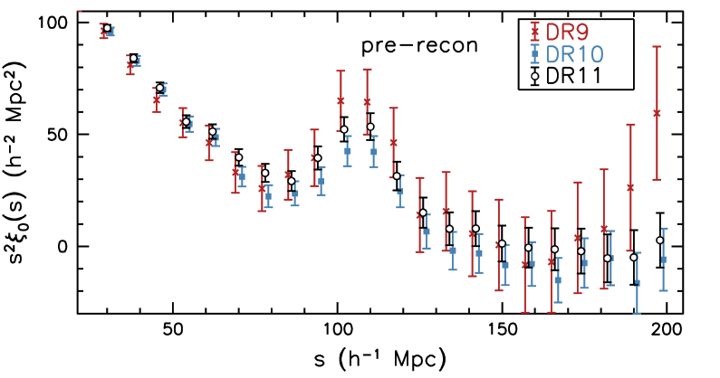
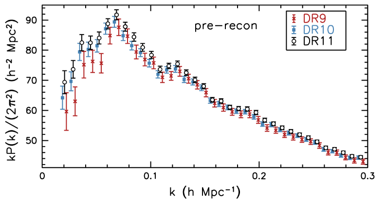
The configuration space and Fourier space clustering measurements made from the DR10 and DR11 CMASS samples are presented in Fig. 10 for and , using our fiducial binning choice. These points are compared against the DR9 clustering results222We recalculate the DR9 using the new method presented in Section 4.1 for consistency. presented in Anderson et al. (2012). For both and , there are variations in the power observed in the different data sets, but the shapes of each are clearly consistent, suggesting that we should expect to recover consistent results for the BAO scale. Measurements of the clustering in the LOWZ sample are presented in Tojeiro et al. (2014).
The power is observed to increase with each data release, and similar behaviour is observed in the correlation function for Mpc. The difference in clustering amplitude can be explained by the tiling of the survey. In order to obtain the most complete sample, dense regions are observed using overlapping plates. Thus, as the survey progresses, a larger percentage of observations using overlapping plates are completed and the mean density of the survey increases. This increase in density occurs almost exclusively by adding over-dense regions and thus increases the clustering amplitude. The measured increase in clustering amplitude is roughly the square of increase in density (4 per cent between DR9 and DR11 and 2 per cent between DR10 and DR11). As the survey nears completion, the issue naturally becomes less important. For DR11, it represents, at worst, a 1 per cent underestimate of the bias of the CMASS galaxies. Consistent trends are found in the LOWZ sample (Tojeiro et al., 2014).
| Estimator | /dof | ||
| DR11 CMASS | |||
| Consensus | (stat+sys) | ||
| + | (stat) | ||
| combined | |||
| combined | |||
| post-recon | 18/27 | ||
| post-recon | 16/17 | ||
| pre-recon | 33/27 | ||
| pre-recon | 14/17 | ||
| DR10 CMASS | |||
| Consensus | (stat+sys) | ||
| post-recon | 23/28 | ||
| post-recon | 14/17 | ||
| pre-recon | 35/28 | ||
| pre-recon | 16/17 | ||
| DR9 CMASS | |||
| Consensus | |||
| DR11 LOWZ | |||
| Consensus | (stat+sys) | ||
| + | (stat) | ||
| DR10 LOWZ | |||
| Consensus | (stat+sys) |
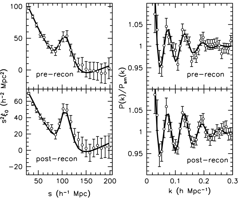
Fig. 11 displays the best-fit BAO model (solid curves) compared to the data for (left panels) and (right panels) for DR11 only. The pre-reconstruction measurements are displayed in the top panels, and the post-reconstruction ones in the bottom panels. The measurements are presented for our fiducial binning width and centring, and show a clear BAO feature in both and , with the best-fit models providing a good fit. The effect of reconstruction is clear for both the correlation function and power spectrum, with the BAO signature becoming more pronounced relative to the smooth shape of the measurements. Indeed, all of the BAO measurements, listed in Table LABEL:tab:isobaoresults, have improved post-reconstruction, in contrast to our DR9 results (Anderson et al., 2012). This behaviour is expected given the results of Section 4.2, which showed that, given the precision afforded by the DR11 volume coverage, reconstruction improved the results from all of our mock catalogues. Reconstruction is particularly striking in the power spectrum plot, showing a clear third peak in the post-reconstruction .
6.2 DR11 Acoustic Scale Measurements
Our BAO measurements are listed in Table LABEL:tab:isobaoresults. The mocks for DR10 and DR11 show significant improvement with reconstruction in most realisations, and we therefore adopt the reconstruction results as our default measurements. Our consensus value for the CMASS BAO measurement, , is determined from a combination of and measurements, and in what follows we describe the process of obtaining this value, and tests that validate it.
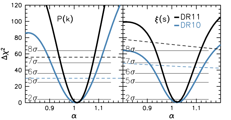
Post-reconstruction, the significance of the BAO detection in both the correlation function and the power spectrum are greater than 7 for the reconstructed DR11 CMASS BAO measurements. The significance of detection is shown in Fig. 12, where we also see a difference in the detection significance between results from and . This variation is caused by the differential ability of the models for the broad-band component to match the offset between the data and the no-baryon model. The broad-band model for the power spectrum has more free parameters than that for the correlation function, so it is perhaps not surprising that the no-baryon model is a slightly better fit.
Table LABEL:tab:isobaoresults also lists /dof for the best-fit models, showing that they are close to unity for DR10 and DR11 fits using both the correlation function and power spectrum. The most unusual is the dof for the post-reconstruction DR11 measurement. Such a low is expected in 10 per cent of cases, thus we conclude that our best-fit models provide adequate descriptions of the data.
The precision of the BAO measurements are typical of those achieved in the mock samples. This consistency in shown in the top panels of Fig. 4, where the orange stars show the uncertainty in the data post-reconstruction versus the uncertainty pre-reconstruction. All of the CMASS data points lie within well the distribution of the mock points. The most discrepant result is for the DR10 measurement post reconstruction; it has an uncertainty of 0.014, while the mean uncertainty from the mock realisations is 0.011, but one can see that many mock realisations recover an uncertainty larger than 0.014.
| Shift | /dof | |
|---|---|---|
| 18/27 | ||
| 19/27 | ||
| 21/27 | ||
| 21/27 | ||
| 20/27 | ||
| 19/27 | ||
| 18/27 | ||
| 16/27 | ||
| 16/27 | ||
| 17/27 | ||
| 12/17 | ||
| 8/17 | ||
| 16/17 | ||
| 14/17 | ||
| 16/17 | ||
| 19/17 | ||
| 17/17 | ||
| 13/17 |
We combine the DR11 CMASS BAO measurements using eight bin centres and the results using ten bin centres in the same manner as applied to the mocks, as described in Section 4.3. The individual fits determined for different bin centres are shown in Table LABEL:tab:binshift. For , our fiducial choice recovered the largest of any of the bin centres. Thus, when combining the results across all of the bin centre choices, decreases to . The uncertainty has decreased by only 2 per cent (compared to the mean of 7 per cent found for the mocks) in part because the estimated uncertainty of the fiducial bin choice (0.0091) is less than the weighted mean uncertainty across all of the bin choices (0.0092). For , the result changes little when we combine across the results of the 10 bin centre choices; it changes from 1.01140.0093 to 1.01100.0093.
We obtain a BAO measurement with an expected error measured from the likelihood surface that is less than 1 per cent for both the reconstructed and . The difference between the two values of is 0.0068. While small in magnitude, this difference is unexpectedly large in the context of the mock results, for which we found a correlation factor of 0.95 between the and results combined across all of the bin choices. Accounting for this correlation factor, the expected 1 dispersion in the and measurements is . The discrepancy in the data is thus 2.4. Comparing to the results from the mocks, we find 7 (1.2 per cent) that have a larger deviation, consistent with our estimation of a 2.4 discrepancy. Both estimates of are stable to a variety of robustness tests, as we will show in Section 6.4, and our tests on mock samples demonstrate that each estimator is unbiased. We therefore conclude that, despite being unusual, the difference between the two measurements is not indicative of an existence of a bias in either measurement.
Our tests on mocks suggest no systematic effects for either the or results when they are obtained by combining results across bin centres. Our methodology applied to mock samples recovers unbiased estimates of the BAO position for both and with nearly identical uncertainty. We therefore obtain the consensus BAO scale measurement by assuming the mean uncertainty of the and measurements for each and using the 0.95 correlation factor. The correct treatment of the data, assuming Gaussian statistics and no systematic uncertainty is to take the mean of and measurements, reducing the uncertainty based on their correlation factor. Thus, our consensus value for the CMASS BAO measurement is , where this uncertainty is purely statistical. Our systematic error budget is discussed in Section 8.1.
We obtain our consensus DR11 LOWZ isotropic BAO measurement, at an effective redshift by applying the same process as applied to CMASS. The details can be found in Tojeiro et al. (2014). The difference in the recovered BAO scale from LOWZ and is within of the expected difference and is opposite in sign to the difference we find for CMASS. The consensus DR11 LOWZ measurement is , considering only the statistical uncertainty.
6.3 DR10 BAO measurements
For completeness, we also include DR10 BAO measurements in Table LABEL:tab:isobaoresults. Post-reconstruction, these data produce a 1.4 per cent BAO scale measurement that is consistent with the DR11 measurements discussed in the previous section. For pre-reconstruction measurements the error on DR11 the result is 30 per cent lower than for DR10. For the post-reconstruction results, the improvement increases to 40 per cent. The reconstruction is more efficient for DR11, which almost certainly results from the more contiguous nature of the DR11 survey mask.
As shown in Fig. 12, the detections for DR10 are both greater than 5, with the significance for the measurement being higher than that of the measurement. As discussed in Section 6.2 the improved detection observed in is because the broad-band model is better able to model the full when no BAO are included, compared with the broad-band model.
The most obvious issue for the DR10 results in Table LABEL:tab:isobaoresults is that, for the DR10 , the measurement of shifts by post-reconstruction, compared to a mean shift of observed in the mocks (here the uncertainty is the standard deviation of the mock values). The size of this shift is thus only just greater than 1 and is consequently not a significant concern.
6.4 DR11 Robustness Checks
| Estimator | Change | /dof | |
| fiducial | 18/27 | ||
| NGC only | 16/27 | ||
| SGC only | 15/27 | ||
| 14/21 | |||
| 11/15 | |||
| 15/23 | |||
| Mpc | 19/28 | ||
| Mpc | 19/28 | ||
| Mpc | 18/28 | ||
| 40/29 | |||
| Spline fit | 17/24 | ||
| 71/79 | |||
| 55/62 | |||
| 33/39 | |||
| 16/20 | |||
| 9/15 | |||
| 5/9 | |||
| 5/6 | |||
| fiducial | 16/17 | ||
| NGC only | 12/17 | ||
| SGC only | 15/17 | ||
| 6/7 | |||
| 24/20 | |||
| 19/19 | |||
| 19/18 | |||
| 18/18 | |||
| free | 15/17 | ||
| 15/17 | |||
| 17/17 | |||
| recon | 11/17 | ||
| recon | 18/17 | ||
| recon | 23/17 | ||
| recon | 14/17 | ||
| 42/38 | |||
| 31/29 | |||
| 19/23 | |||
| 20/19 | |||
| 10/14 | |||
| 9/12 |
In order to ensure that our measurements on the CMASS data are robust to our methodological and binning choices, we re-measure the BAO scale using the reconstructed DR11 power spectrum and correlation function, changing the fitting methods, binning and fitting to the NGC and SGC separately. Table LABEL:tab:isorobust lists the results of these tests.
The absolute difference in the values recovered from the NGC and SGC regions has decreased considerably from Anderson et al. (2012). For the correlations function fits, the decrease if from to . Given the decrease in the uncertainty thanks to the larger area coverage in both regions, the significance of the discrepancy is similar to that found for DR9, 1.4. We find 79 out of the 600 mock samples (13 per cent) have a larger discrepancy, consistent with the estimation of a 1.4 discrepancy. We find a similar picture when we fit to the measurements from NGC and SGC although, in this case, the discrepancy is slightly larger, at 1.8. Less significant differences, with opposite sign, are found in the DR11 LOWZ sample (Tojeiro et al., 2014).
Table LABEL:tab:isorobust also presents results fitting to the power spectrum for different ranges in , removing the largest and smallest-scale data in turn. The recovered errors on do not change significantly if we remove data at or at . This is not surprising, given there is little BAO signal on these scales. Only fitting to reduces the best-fit value of by , but cutting further in to returns the best fit back to the fiducial value, suggesting that there is no wavelength-dependent systematic trend present. Fixing the BAO damping at the best-fit value from the mocks Mpc does not alter the best-fit value of , but does decrease the size of the error, but we consider this action to be too aggressive given that the true value of the damping is unknown. Changing by Mpc does not have a large effect, although overdamping the BAO in the model does increase the error on , as it removes the signal we wish to match to the data.
Results from applying two alternatives to the model for the broad-band power spectrum shape are also shown: Cutting the polynomial model back to a 4-parameter model by setting and in Eq. 24 only slightly affects and the recovered error, but does significantly increase the best-fit value of , showing that this model inadequately describes the shape of the power. Changing to the bicubic spline broad-band model used previously (Anderson et al., 2012) does not significantly affect either the best-fit value of or the recovered error.
Table LABEL:tab:isorobust also presents results reducing the range of scales fitted in the correlations function from to : we find a negligible change in the best-fit value of , and a revised error that only increases by a small amount, demonstrating that this reduced range of scales contains all of the BAO signal as expected. We also present results from possible changes to the model used to fit the broad-band correlation function, where we remove various polynomial terms, or remove the prior on (Eq. 27). The greatest change is an increase in the recovered value of 0.0023 when only the constant term is used to fit (Eq. 28). Indeed, for , the preference for the inclusion of a polynomial is not strong; for three additional parameters. While the correlation function adds terms to a full linear model (Eq. 27), the power spectrum only includes the BAO component (Eq. 23), which is why the polynomial term is less important for . As we did for the power spectrum, we vary the non-linear BAO damping, finding consistent results.
The reconstruction algorithm requires an assumed amplitude for the real-space clustering of the galaxy field () and its associated velocity field (). In the fiducial case, we assume and , which are measured from the mocks. However, our results are not sensitive to these assumptions: if we change each by per cent and re-calculate the reconstructed field for the DR11 data and re-determine , the resulting measurements of show negligible change.
For both the power spectrum and correlation function, Table LABEL:tab:isorobust also presents results where we change the bin size, revealing significant scatter. The equivalent comparison for the mock catalogues was presented in Percival et al. (2014). For both and measured from the data, a dispersion of 0.002 is found in the best-fit values. The weighted mean across bin sizes (accounting for the covariance between bins) is 1.01800.0089 for and 1.01170.0091 for . These measurements are similar to the results obtained when combining across bin centres, suggesting the combined bin centre results largely capture the same information as changing the bin size. The bin size recovers . While this value is significantly larger than any of the other bin sizes, this bin size has a relatively small correlation factor, 0.8, with the weighted mean of the other bin sizes. It is thus only 1.2 from the BAO fit to averaged into narrower bins.
For all of the tests presented in this section, we find no evidence for changes in the best-fit value of that are sufficiently outside of the statistical expectation to indicate the presence of systematic effects. The most significant discrepancy we have observed is the different values of recovered from and , but the robustness checks presented in this section have not pointed to any origin for this difference, other than simply it being a statistical fluctuation.
6.5 Displaying the BAO Feature
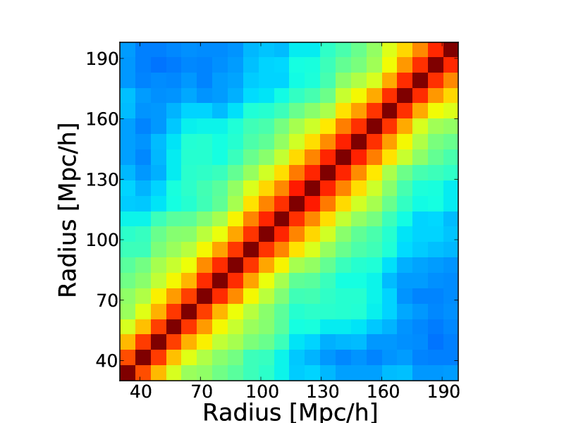
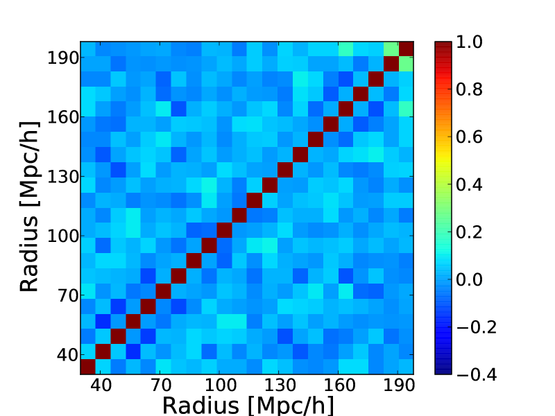
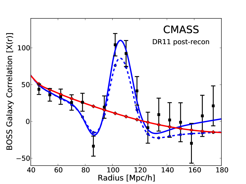
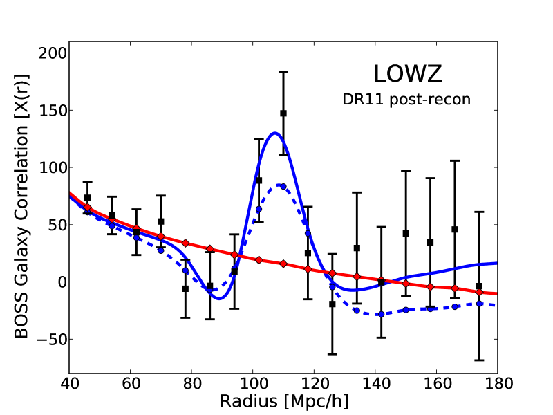
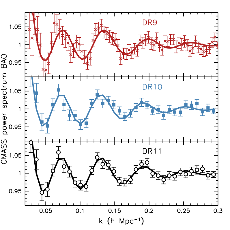
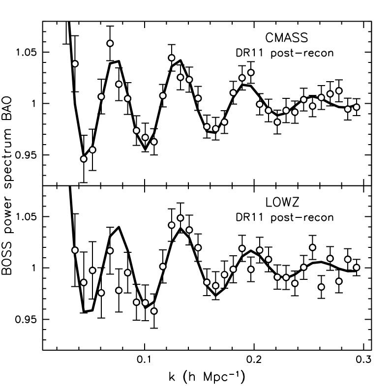
Plots of the two-point clustering statistics can be difficult to interpret because of the correlations between the data points. This effect is particularly severe for the correlation function: as the density of the data set increases, different scales become heavily correlated. For example, fluctuations in the amplitude in poorly constrained modes of very low wavenumbers cause the entire correlation function to shift up and down. This means that the diagonal of the covariance matrix is a poor representation of the actual uncertainties. In the case of the acoustic peak, this leads to the data being more constraining than it appears! This effect is of no consequence for the formal analysis—one simply uses the covariance matrix when fitting models—but it is a challenge for pedagogy.
The correlations of estimators can be avoided by adopting a new basis, i.e., choosing new estimators that are linear combinations of the original correlation function bins. Such transformations are extensively discussed in Hamilton & Tegmark (2000). There are an infinite number of choices of bases that will produce diagonal covariance matrices. The pedagogical challenge is that the new estimators now represent a mixture of all scales and hence it is not clear how to plot the measurements.
Here, we present a hybrid approach in which one adopts a simply-defined estimator with compact support as a function of scale, but chooses the estimator so that the covariances are significantly suppressed. In particular, Hamilton & Tegmark (2000) noted that transformations based on the symmetric square root of the Fisher matrix had surprisingly compact support for their power spectrum analysis. When we formed this matrix for the DR11 CMASS correlation function, we found that the first and second off-diagonal terms are nearly constant and that subsequent off-diagonals are small. This suggests that a basis transform of the pentadiagonal form
| (46) |
will approach a diagonal form. Here, and is the bin center of measurement bin . We introduce the factor so as to normalize such that it returns for constant . For the first two and last two bins, the terms beyond the end of the range are omitted and the normalization adjusted accordingly.
We find that for DR11 CMASS after reconstruction, values of and sharply reduce the covariances between the bins. The reduced covariance matrices for and are shown in Figure 13. The bins near the edge of the range retain some covariances, but the off-diagonal terms of the central submatrix of the reduced covariance matrix have a mean and r.m.s. of , with a worst value of 0.11. For display purposes, this is a good approximation to a diagonal covariance matrix, yet the definition of is well localized and easy to state. For comparison, the reduced covariance matrix of has typical first off-diagonals values of 0.8 and second off-diagonals values of 0.6.
We display this function in Figure 14. One must also transform the theory to the new estimator: we show the best-fit BAO models with and without broadband marginalization, as well as the best-fit non-BAO model without broadband marginalization. The presence of the BAO is clear, but now the error bars are representative. For example, the significance of the detection as measured by the of the best-fit BAO model to the best-fit non-BAO model is 69.5 using only the diagonal of the covariance matrix of , as opposed to 74 with the full covariance matrix. We do not use this transformation when fitting models, but we offer it as a pedagogical view.
The same result is shown for DR11 LOWZ post-reconstruction in Figure 15. Here we use and . The level of the off-diagonal terms is similarly reduced, with an r.m.s. of 3.4 per cent and a worst value of 12 per cent.
It is expected that the best values of and will depend on the data set, since data with more shot noise will have covariance matrices of the correlation function that are more diagonally dominant. Similarly, the choice of a pentadiagonal form may depend on the binning of the correlation function, as it likely reflects a physical scale of the covariances between bins. However, some of the simplicity likely results from the fact that the covariances between nearby bins are dominated by small-scale correlations in the density field that become independent of separation at large separation. This property gives the matrix a regularity: bins at 90 and Mpc will be correlated to each other similarly to bins at 110 and Mpc. Tridiagonal matrices have inverses with exponentially decreasing off-diagonal terms (Rybicki & Press, 1995). Apparently, treating the off-diagonal covariances as exponentially decreasing with only weak dependences on separation provides a good approximation.
For , the measurements in -bins are already fairly independent, as one would expect for a near-Gaussian random field. Correlations between bins can occur because of the finite survey volume and because of non-Gaussianity in the density field. For CMASS, we find the mean first off-diagonal term of the reduced covariance matrix is 0.28 (with a standard deviation of 0.06). When the measurements are divided by the best-fit smooth model, , they are, generally, even less correlated. We determine for each mock sample and construct a revised “BAO” covariance matrix from this. We do not use this covariance matrix to perform any fits—our fits are to the full and use the original covariance matrix. For the revised covariance matrix, the mean first off-diagonal term of the correlation matrix is reduced to 0.03 (with a standard deviation of 0.15). The diagonal elements within this covariance matrix are also reduced in amplitude, reflecting the smaller variance available once a smooth fit has been removed. The errors derived from this matrix thus better represent the errors on the measured BAO; the data when presented as are more independent and provide a more accurate visualisation of the measurements.
Fig. 16 displays the measured post-reconstruction values of , for the BOSS CMASS sample in DR9, DR10, and DR11 (from top to bottom), showing the evolution in the signal-to-noise ratio of the BAO as BOSS has increased its observed footprint. In the DR11 sample, the third peak is clearly visible. In Fig. 17, we display the DR11 post-reconstruction for the two BOSS samples; the CMASS sample at is presented in the top panel and the LOWZ sample at is shown in the bottom panel. The LOWZ sample possesses a clear BAO feature, but the signal-to-noise ratio is considerably lower than that of the CMASS sample.
7 BAO Measurements from Anisotropic Clustering Estimates
7.1 Anisotropic Clustering Estimates
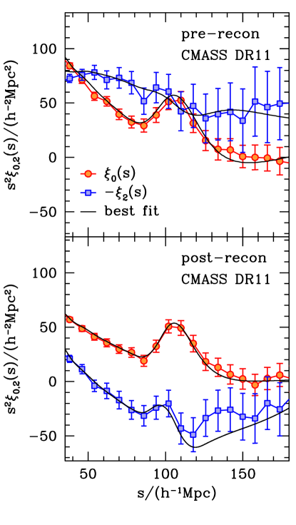
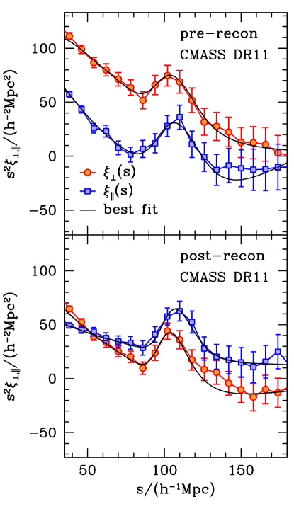
In Section 5, we detailed our analysis techniques (multipoles and wedges statistics), and demonstrated they recover un-biased estimates of the BAO scales both along and perpendicular to line-of-sight with similar uncertainties. We now apply these two techniques to BOSS CMASS sample (at ). Fig. 18 displays the multipoles, , of the DR11 CMASS sample correlation function pre- and post-reconstruction, using our fiducial binning choice, for the range of scales fitted (). For the quadrupole (), we see a dramatic change from the pre- to post-reconstruction results, as the reconstruction algorithm has removed almost all of the redshift space distortion contribution. Further, an apparent dip is now seen in the data on scales slightly larger than the peak in the monopole. The strength of this feature is related to the deviation in from 0 (or the deviation in from 1).
Fig. 19 displays the correlation function divided into two wedges (), once again with the pre-reconstruction measurements displayed in the top panel and the post-reconstruction measurements in the bottom panel. Reconstruction has made the BAO peak sharper for both and . Further, reconstruction has decreased the difference in their amplitudes as the redshift space distortion signal has been reduced.
7.2 DR11 Acoustic Scale Measurement from Anisotropic Clustering
As for our isotropic analysis, the results of our anisotropic BAO fits to the DR10 and DR11 mocks show significant improvement on average with reconstruction (see Table 5), and therefore we adopt post-reconstruction results as our default. Our consensus value for the CMASS anisotropic BAO measurement, , , is determined from a combination of the measurements using the multipoles and the wedges methodologies, and we describe the individual measurements and the process of arriving at our consensus measurement in what follows.
The curves in Figs. 18 and 19 show the best-fit BAO models333The best fits to both where and respectively. to the pre- and post-reconstruction data using the multipoles and wedges methodology. The fits, with characteristics listed in Table 10, provide a good description of the data for 30 dof: the largest is 35 (a larger would be expected 24 per cent of the time) and the smallest is 21 (a smaller would be expected 11 per cent of the time).
The uncertainties on the anisotropic BAO measurements are typical of those we find in the mock samples. For the multipoles result, this is illustrated in Fig. 7, which shows that the uncertainties recovered from the data (orange stars) are within the range of those recovered from mock samples (blue points). The uncertainty on the BAO measurements using the wedges methodology are similar to the multipoles results, with a small increase for , that exactly matches that seen fitting mock catalogues. We further illustrate the constraints obtained from each method in Fig. 20 where one can see the comparison of the 60 per cent and 95 per cent constraints in the and plane scaled by using the two methods. The size of the contours from both methods agree very well, with a slightly more elongated contour from multipoles, showing that the multipoles and wedges contain slightly different information.
The precision of the DR11 results are improved by reconstruction, as expected. This is illustrated in Fig. 20, where the post-reconstruction , contours in the right-hand plot show a dramatic decrease compared to the pre-reconstruction results displayed in the left-hand panel. Based on our testing of 600 mock CMASS samples, we found (as shown in Figure 7) that reconstruction is expected to improve the precision of the multipoles method measurement of by per cent (the median uncertainty decreases from 0.021 to 0.015) and of by 63 per cent (the median uncertainty decreases 0.044 to 0.027), with very similar results using the wedges methodology. We find that for the DR11 data, the results are similar to our expectation, as the improvements in the precision of the results gained by reconstruction are all between 39 and 50 per cent. The improvement in (50 per cent for multipoles and 42 per cent for wedges) is slightly better than expected and the improvement in (39 per cent for multipoles and 48 per cent for wedges) is slightly worse, but Fig. 7 shows that the results (orange stars) are well within the range of the results determined from mock samples (blue points).
Table 10 shows that the DR11 post-reconstruction multipoles and wedges results disagree by close to 1-: , ; , . The difference in is . We then turn to the galaxy mock catalogs to see whether this behavior is common. We find that 39 out of 600 mocks show the same or larger differences between the two methods. The mean difference is with a RMS of suggesting that this difference in the data is a 1.9 event. The difference in is , we also found 45 out of 600 cases that show the same or larger differences between the two methods. The mean difference found in the mocks is and the r.m.s. is , this suggests that the difference in the data is a 1.6 event. This is mostly driven by differences in the fitted results of , Table 10 shows us that the fitted values of from both methodologies only differ by per cent, while is different by per cent, which is comparable to the 1 error on . We thus turn to a discussion using - parametrization in the following discussion.
Pre-reconstruction, the multipoles and wedges measurements in and differ by less than 0.25 as shown in Table 10. Fig. 20 shows that, as reconstruction tightens the constraints from both methods, the central values shift slightly along the axis of constant by per cent in . When we look at this comparison in our mocks, we find a r.m.s. difference in fits of , indicating that the data is a outlier. of 600 mocks have differences more extreme than . The other three cases (DR10 and DR11 pre-reconstruction) show smaller variations. We conclude that this event is consistent with normal scatter of the two estimators.
Our tests on our fitting methodology, presented for the mock samples in Section 5.2 and on the DR11 data in Section 7.3 suggest no systematic issue causing the observed difference between the results of the two methods. Thus, we combine the likelihood distributions recovered from the multipoles and wedges measurements, using the method described in Section 5.3, to recover our consensus anisotropic BAO measurement, and . We quote the statistical and systematic error444The systematic errors are described in Sec 7.3 and Sec 8.1. The addition of the two types of error is described in Sec 8.1. here for consensus values, while the remaining values in Table 10 consider only the statistical errors.
| Model | ||||||||
| DR11 | ||||||||
| Consensus | 1.0190.010 | -0.0250.014 | 0.390 | 0.9680.033 | 1.0450.015 | -0.523 | - | |
| Post-Recons. Multipoles | 0.505 | -0.311 | ||||||
| Post-Recon. Wedges | 0.389 | -0.501 | 21./30 | |||||
| Post-Recon. De-Wiggled | -0.304 | |||||||
| Post-Recon. Isotropic | – | – | – | – | - | |||
| Pre-Recon. Multipoles | 0.495 | -0.246 | ||||||
| Pre-Recon. Wedges | 0.236 | -0.453 | 33/30 | |||||
| Pre-Recon. De-Wiggled | 0.572 | -0.149 | ||||||
| Pre-Recon. Isotropic | - | - | - | - | - | |||
| DR10 | ||||||||
| Consensus | 1.0190.015 | -0.0120.020 | 0.502 | 0.9940.050 | 1.0310.019 | -0.501 | - | |
| Post-Recon. Multipoles | 0.683 | -0.240 | ||||||
| Post-Recon. Wedges | 0.513 | -0.474 | 17/30 | |||||
| Post-Recon. De-Wiggled | 0.669 | -0.163 | 16./30 | |||||
| Post-Recon. Isotropic | – | – | – | – | – | |||
| Pre-Recon. Multipoles | 0.439 | -0.346 | ||||||
| Pre-Recon. Wedges | 0.104 | -0.482 | 30/30 | |||||
| Pre-Recon. De-Wiggled | 0.555 | -0.237 | ||||||
| Pre-Recon Isotropic | – | – | – | – | - |
| Method | /d.o.f | ||||||||
|---|---|---|---|---|---|---|---|---|---|
7.3 Robustness Checks on Data
We measure the DR11 post-reconstruction anisotropic BAO scale with various choices of methodology, in order to test the robustness of our anisotropic BAO measurements. Because of the tight correlation between results calculated from fits to either multipoles or wedges (see Section 5.2), we only present robustness checks for fits to the multipoles. We have only summarized the results of the robustness that are of immediate relevance to this paper here, while the full robustness test of our anisotropic BAO fitting methodology is shown in Vargas-Magana et al. (2013).
We vary the choices when fitting to the data in the same way as we did when testing the results on the mock samples in Section 5.2. The results are summarized in Table 11 and we can see that the differences in central fitted values when we consider different choices of fitting parameters are impressively small. The central fitted values of vary less than per cent, while the various fitted errors vary less than per cent. For all cases but one, the central fitted values of vary less than per cent, while the fitted errors vary less than per cent. The largest variation found is on when we we change the broadband polynomial such that each component () is only limited to 2-terms, which is still relatively small, at per cent, which is less than . We can turn our attention to and , but as expected, since the variations are not large for and , the changes in and are equally small.
We also investigate the effects of priors. We refer the reader to the priors listed in Section 5.1. In both mocks and data of DR11 post-reconstructed, we find that as long as we either limit the to reasonable physical intervals when we calculate the error or use priors on both and , the final fitted central values and errors remain relatively unchanged to within per cent. We have discussed this further in a companion paper (Vargas-Magana et al., 2013), which should be consulted for more details. Finally, it is also interesting to note that a fixed parameter does not change the error or central values by more than per cent. To conclude, the variations of DR11 post-reconstructed data is well within the scatter predicted when the same varying choices are applied to mock galaxy catalogs.
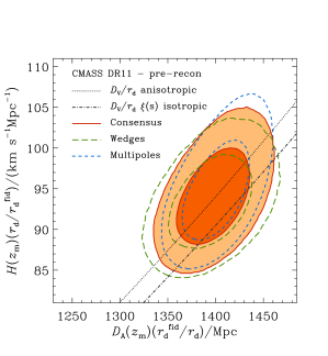
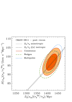
7.4 DR10 Anisotropic BAO measurement
Although our default results are for DR11, it is instructive to examine the results from the reduced DR10 data set, which allow us to follow the transition in data quality from our previous DR9 results to our new DR11 results. Consequently we present anisotropic BAO measurements from DR10 alongside the DR11 measurements in Table 10. For the mock catalogues, Fig. 7 showed that, for fits to the DR10 multipoles, the expected improvement of the measurement in and with reconstruction is from per cent and per cent to per cent and per cent respectively. Using the DR10 data, we measure and pre-reconstruction. Post-reconstruction, we measure and , showing remarkable consistency with the mock results. The measurement using wedges, also presented in Table 10, are similar and consistent. Thus the precision of the BAO measurements from the DR10 data are typical. This can also be seen in Fig. 7, where the orange star representing the data results is within the locus of the blue circles representing results from the mocks.
It is interesting that, for DR10, the error post-reconstruction is slightly larger for , compared with the pre-reconstruction error. We can see this more clearly by looking at the and pair pre- and post-reconstruction in DR10 in Table 10. It seems there is no improvement in , while there is some slight improvement in post-reconstruction. We compare this to the mocks to try and understand this behaviour. Figure 7 shows that not all mocks in DR10 have improved constraints on after reconstruction, even though it is uncommon: out of 600 mocks that do not improve. We do see improvement on nearly all mocks in DR11, which may be due to the fact that DR11 has a more contiguous mask, so that there is less volume close to boundaries. This may contribute to a more successful reconstruction in DR11.
7.5 Comparison with Isotropic Results
For ease of comparison between our isotropic and anisotropic measurements, we include the results from isotropic fits to the correlation function (presented in Table LABEL:tab:isobaoresults) in Table 10. Post-reconstruction, the central values of measured from isotropic and anisotropic clustering are consistent to well within 1-. Pre-reconstruction, the central values of from the isotropic correlation function are approximately 1- higher than from the anisotropic clustering , for both DR10 and DR11. Part of this difference can be explained by the different correlation function templates used for the isotropic and anisotropic analyses. The anisotropic fitting uses as described in Eq 38 which was chosen as it provides less biased measured values of and fitting, while the isotropic fitting uses a non-linear power-spectrum “De-Wiggled template” Anderson et al. (2012, 2014). The differences though between the templates are quite small and are further explored in Vargas-Magana et al. (2013). For comparison, we provide anisotropic fits made using the same “De-Wiggled” power spectrum template used for the isotropic fits in Table 10, it is not surprising that the anisotropic results with the same power spectrum template provides more similar fits to those from the isotropic fits in both pre-reconstruction and post-reconstruction datasets (this is explored further in Vargas-Magana et al. 2013).
For DR11 post-reconstruction, which is our default choice for making cosmological measurements, we note that the isotropic power spectrum fits give lower values of than the isotropic correlation function fits, pulling the isotropic consensus values of down (see Table LABEL:tab:isorobust). On the other hand, the correlation function monopole measurement of agrees very well with the values measured from anisotropic fits to both the monopole and the quadrupole. They are both higher than the consensus value of the isotropic fits (a combination of both isotropic power-spectrum fit and the correlation function fit), and the effect of this is noticeable when the measurements are combined with the CMB data and turned into cosmological constraints (see Fig. 23 and Section 9.2).
Isotropic fits of only allows us to measure the spherically averaged distance , where z is the median redshift of the sample. This has made the approximation that the clustering of the galaxy sample is isotropic. More importantly, the Hubble parameter is degenerate with in this isotropic measurement, and thus we cannot directly probe the expansion of the Universe. The clustering of galaxies is not truly isotropic due to both large-scale redshift-space distortions and from assuming the wrong cosmology when we calculate the 2-point statistics. Therefore, the fit to the anisotropic clustering provides more information by breaking the degeneracy between and . We are therefore not surprised that the anisotropic clustering measurements provides stronger cosmological constraints as demonstrated by the different contour sizes in Fig. 23. We further compare and contrast the isotropic and anisotropic fits in Figure 20. While on average the anisotropic degeneracy direction should lie along the isotropic () direction, in our data set the orientation is closer to vertical. This slight rotation is driven by the shot-noise differences along the line of sight and perpendicular to the line of sight. This is expected, given the comparison of the data and ensemble of mock constraints on and shown in Fig. 7. This figure also illustrates the 0.5 per cent increase in the best-fit from the anisotropic fits compared with the isotropic ones. Anisotropic clustering’s constraining power is also amplified depending on the models we explore. For example, variation in dark energy equation of state () shifts at fixed CMB acoustic scale, and anisotropic clustering measurements provide stronger constraints than isotropic ones in the direction of (Fig. 20).
Therefore, we choose the anisotropic clustering measurements to be the default measurement of the CMASS measurement in our cosmological analysis (thus will only be referred to as CMASS in later sections).
8 The Cosmological Distance Scale
8.1 Systematic Errors on BOSS BAO Measurements
Sections 4 and 5 presented the acoustic scale fits and their statistical errors. Here we present estimates of systematic errors, which we believe to be subdominant by a considerable margin. We organize the discussion into two separate classes of systematic errors. The first set includes possible artifacts from our survey, including the effects of survey boundaries and observational systematics on the reconstruction and fitting methodology. The second set concerns the possible residual effects of galaxy clustering bias on the shift of the acoustic scale after one applies our reconstruction algorithm assuming a large filled survey.
As shown in Table LABEL:tab:mockbao, when run on our mock catalogs, the estimators for both the spherically averaged correlation function and the power spectrum return unbiased results in DR11 after reconstruction, with precision of 0.04 per cent in the mean. Table 5 and Table 6 show that when we run our different estimators (Multipoles and Wedges) for the anisotropic clustering signals on mock catalogs they return unbiased results in DR11 both pre-reconstruction and post-reconstruction. This is an extremely sharp test, as it includes the effects of the survey geometry and ability of reconstruction to remove the non-linear shifts of the acoustic scale that arise from Lagrangian perturbation theory as used in our mocks. It also validates our fitting methodology, e.g., demonstrating that effects of binning, interpolation, and integrations in the measurement and fitting procedures have been handled well. Ross et al. (2014) use two other sets of mocks, using the same formalism as Manera et al. (2013a) but with different halo mass cuts; they find similar unbiased performance after reconstruction, with precision better than 0.1 per cent.
The effects of variations in the fitting methodology was discussed in sections 6 and 7, showing only small offsets, at the level of 0.1-0.2 per cent in for cases that were expected to agree. Anderson et al. (2012), Anderson et al. (2014), and Vargas-Magana et al. (2013) present further tests, again finding no substantial offsets.
One can also search for systematic errors by comparing different aspects of our analysis. Indeed, we do find cases in which different analyses of the same data return acoustic scales that differ by of order 0.5 per cent, e.g., the comparison of the measured from and in DR11. However, these discrepancies occasionally occur in our mock catalogs and hence are not sufficiently unusual to indicate a systematic error, particularly because we examined a substantial number of these comparisons, many of which were unremarkable. If these differences are indeed due to systematic effects, then it must be for reasons that are not present in our mock catalogs, as each of our estimators is unbiased when averaged over many mocks.
The mocks do not include large-angle observational systematics due to such things as variations in star-galaxy separation effectiveness or seeing, as were discussed in Ross et al. (2012). However, the acoustic peak measurement is highly robust to such effects, as they tend to have smooth angular power spectra. One would expect that if such effects were present, they would be much more severe if we omitted the broadband nuisance terms described in § 4. As shown in § 6, performing our correlation function fits with fewer or even none of the three broadband nuisance terms produces changes in of 0.2 per cent or less. Removing two terms from the power spectrum fit also changes the answer by only 0.2 per cent.
Although we measure the clustering within a redshift bin of non-zero thickness, we interpret the fitted scale as measuring the distance to a single effective redshift. We base this estimate on the mean redshift of fully weighted pairs, rounded off for simplicity. This effective redshift is not formally well defined—for example, it might depend on scale or differ between line-of-sight and transverse clustering—but different reasonable choices vary by only 0.01 in redshift. We then expect the effect of this assumption to be small because any error in the effective redshift enters only as the variation with redshift in the ratio of the true cosmology to the fiducial cosmology. For example, we will see in § 9 that the ratio of between the best-fit CDM model and a model with that matches the CMB data varies by about 1 per cent for each 0.1 in redshift. This would be a 0.1 per cent shift for an 0.01 change in effective redshift. Yet this much tilt in the distance-redshift relation is already disfavored by the BAO Hubble diagram and by the supernova data. Hence, we argue that errors in the effective redshift affect our interpretations at below 0.1 per cent.
Similarly, our mocks are based on a single redshift snapshot of the simulations, rather than light-cone outputs that track the exact structure at each redshift. This approach could create errors when we combine a broad redshift bin into one clustering measurement and interpret the acoustic peak as arising from a single, effective redshift. Note that the amplitude of galaxy clustering changes much more slowly than the predicted variation in the amplitude of the matter clustering, which limits the mismatch of combining different redshifts. Preliminary tests of this approximation with light cone simulations in a few cases show the effects to be small, but we intend to extend these tests in the future.
The choice of fiducial cosmology also enters through the linear power spectrum used in our fitting. The assumption of our methodology is that the values recoved from fits with other template spectra would be well predicted by the ratios of sound horizons computed in these cosmologies to that of the fiducial model. Were this not the case, we would simply have to repeat the fit for each new cosmology, searching for cases of . This assumption has been investigated in previous papers and found to be a good approximation (Seo et al., 2008; Xu et al., 2012a, b), with systematic offsets typically at or below 0.1 per cent in . One exception was presented in Xu et al. (2012a), where a case with an extra relativistic neutrino species created an uncorrected 0.5 per cent shift of due to template mismatches. Hence, more exotic cosmologies may require additional consideration of whether the sound horizon fully captures the impact of the variation in the fitting template.
Our conclusion from these tests is that there is no evidence for systematic errors from the survey effects and fitting above the 0.1 per cent r.m.s. level from any effect we have considered. However, there are several such terms that could accumulate, so we triple this to adopt a systematic error of 0.3 per cent for our measurements of . We believe that further tests on a more diverse and realistic set of mock catalogs would boost confidence in the methods at the 0.1 per cent aggregate level.
The analysis of the anisotropic BAO could be subject to additional systematic errors due to the above effects. The anisotropic fitting is more complicated because of redshift distortions and the inherent anisotropy of the survey geometry and light-cone effects. Our tests on mock catalogs show the estimators to be unbiased at the level of 0.2 per cent in . Vargas-Magana et al. (2013) presents an exhaustive set of tests of the multipole fitting method; Xu et al. (2012b), Anderson et al. (2014), and Kazin et al. (2013) present a wide variety of tests on earlier data sets. For the DR11 post-reconstruction case, Vargas-Magana et al. (2013) find variations in at the 0.1-0.2 per cent level as the parameters in the fitting method are varied. We take these results to indicate a 0.3 per cent r.m.s. systematic uncertainty in due to fitting. We increase this estimate to 0.5 per cent to include possible errors in the anisotropic BAO external to our mocks, e.g., due to light cone effects, evolution in the sample, inaccuracies in assumptions about peculiar velocities in the mocks or reconstruction, or mismatches between our fiducial cosmology and the true one.
Our estimate of statistical error does depend on the assumption that the amplitude of clustering in the mocks matches that in the true data, as the sample variance of the density field depends on its power spectrum. Our current mocks have about 10 per cent less power than the data, which might lead to a small underestimate of the sample variance in the correlation function. The variance of the power spectrum analysis would actually be slightly overestimated because the covariance matrix was computed for and hence includes only the fractional error on the power. The fractional error would be somewhat larger because of the increased importance of shot noise relative to a weaker clustering signal. The fact that the effects of a mismatch in clustering amplitude have opposite effects on the estimated errors in and , combined with the result that the uncertainties in recovered from each statistic match closely, further argues that this effect is small. At present, we make no correction to our statistical error bars for the offset of clustering amplitude in our mocks, as the mismatch is small and the exact size of the resulting correction not well known. We also do not include a term in our systematic errors for possible mismatches of the amplitude of clustering, as this does not represent a bias in the mean, but rather an error on the error.
We next turn to systematic errors from true astrophysical shifts due to non-linear structure formation and galaxy clustering bias. Prior to reconstruction, one can see the small expected shift, of order 0.4 per cent, in the fitting of the mocks. From perturbation theory (Crocce & Scoccimarro, 2008; Padmanabhan & White, 2009) and simulations (Padmanabhan & White, 2009; Seo et al., 2010) we expect shifts in the clustering of matter at 0.2-0.25 per cent at these redshifts. Galaxy bias produces additional small shifts (Padmanabhan & White, 2009; Mehta et al., 2011). As reconstruction improves due to the larger and more contiguous survey volume, we expect it to remove the shifts due to large-scale velocities. Mehta et al. (2011) found no example in their models in which the shift after reconstruction was non-zero, with errors of about 0.1 per cent r.m.s.. The mock catalogs used here, as well as the two in Ross et al. (2014), also show no offsets at this level. Of course, our mock catalogs and the galaxy bias models of Mehta et al. (2011) do not span all possibilities, but there is a good physical reason why reconstruction is successful at removing shifts: in a wide range of bias models, the galaxy density field is proportional to the dark matter density field at scales above Mpc. The shifts in the acoustic scale arise in second-order perturbation theory due to large-scale flows, which are well predicted by the galaxy maps. Reconstruction substantially reduces the flows and hence the source of the acoustic scale shifts. To be conservative, we triple the level of uncertainty implied by our current mocks and adopt a systematic error of 0.3 per cent in for shifts from galaxy bias that are not corrected by reconstruction.
Our systematic error budget for galaxy clustering bias does not encompass offsets that could result from the effects of relative streaming velocities between baryons and dark matter in the earliest collapse of proto-galaxies (Tseliakhovich & Hirata, 2010). Although this effect is large at the cosmological Jeans scale of halos, the galaxies we measure in BOSS occupy halos over a million times larger and one might imagine that the impact of the early streaming velocities have been significantly diluted. Empirically, a recent paper by Yoo & Seljak (2013) limited the acoustic scale shifts from this effect through its impact on the large-scale DR9 power spectrum; they found a remaining r.m.s. uncertainty of 0.6 per cent. While we look forward to more work on the possible effects of relative streaming velocities, we do not inflate our systematic errors by this much, as theories often predict the effect to be negligible at mass scales well above the cosmological Jeans scale (see e.g. McQuinn & O’Leary, 2012).
To summarize, for our isotropic analysis, we adopt systematic errors of 0.3 per cent for fitting and survey effects and 0.3 per cent for unmodeled astrophysical shifts. These are applied in quadrature. These systematic errors increase the error on the CMASS consensus value from 0.9 per cent to 1.0 per cent and the error on the LOWZ consensus value from 2.0 per cent to 2.1 per cent. For the anisotropic analysis, we apply the above effects in quadrature to and then add an additional independent systematic error of 0.5 per cent in quadrature to . The impact on the measurement of and is subdominant to the statistical errors.
| Comparison between different CMASS-DR11 results | ||||
|---|---|---|---|---|
| source | method | |||
| this analysis | consensus | |||
| Beutler et al. (2013) | -multipoles | |||
| Samushia et al. (2014) | -multipoles | |||
| Chuang et al. (2013b) | -multipoles | |||
| Sánchez et al. (2013b) | -wedges | |||
8.2 The Distance Scale from BOSS BAO
As described in Anderson et al. (2012) and Anderson et al. (2014), the value of is directly related to the ratio of the quantity to its value in our fiducial model:
| (47) |
Similarly, and measure the ratios of and , respectively, to their values in our fiducial model.
We opt to quote our results by writing these quantities as
| (48) | |||||
| (49) | |||||
| (50) |
With this form, we emphasize that only the ratio of between the adopted and fiducial cosmology matters. There are a variety of possible conventions and fitting formulae available for ; any of these can be used so long as one is consistent. Moreover, within the usual class of CDM cosmologies, the CMB data sets tightly constrain . For example, the Planck Collaboration (2013b) results imply to 0.4 per cent r.m.s. precision for the minimal CDM model and extensions to spatial curvature and low-redshift dark energy. As this is somewhat tighter than our statistical errors on the ’s, it is reasonable to choose a form of the results that emphasizes the absolute measurement of the distance scale.
The effective redshift of CMASS is , while that of LOWZ is . Our fiducial cosmology is , km s-1 Mpc-1, , , eV, , , and . Using this cosmology, we obtain Mpc, Mpc, and km s-1 Mpc-1 for CMASS. For LOWZ, we have Mpc, Mpc, and km s-1 Mpc-1.
Inserting the constraints on , we find the primary isotropic results of this paper:
| (51) | |||||
| (52) |
for the post-reconstruction DR11 consensus values. For the anisotropic CMASS fit, we find
| (53) | |||||
| (54) |
with a correlation coefficient between and of 0.539 (in the sense that higher favors higher ). As described in Section 7.5, we recommend the anisotropic values as our primary result at when fitting cosmological models.
When applying these constraints to test cosmology, one must of course consider the variation in the sound horizon in the models. Our fiducial cosmology has a sound horizon Mpc if one adopts the definition in Eqs. 4 through 6 of Eisenstein & Hu (1998, hereafter, EH98). Alternatively, if one adopts the definition of the sound horizon in Camb, one finds Mpc, which is 2.6 per cent less. Much of the past BAO literature uses the EH98 convention, but we now recommend using Camb as it provides a transparent generalization to models with massive neutrinos or other variations from vanilla CDM. As discussed in Mehta et al. (2012), the ratio of the EH98 and Camb sound horizons is very stable as a function of and , varying by only 0.03 per cent for the range and . Thus in evaluating the ratios that appear in our expressions for , , and , the choice is largely irrelevant. We further find that for , and eV, the approximation of
| (55) |
matches Camb to better than 0.1 per cent, whatever the mass hierarchy. One can use any of these conventions for the sound horizon in applying our results, so long as one is consistent in evaluating and .
For comparison to past work, using the EH98 sound horizon, we find and . Using the Camb sound horizon instead, this shifts to and .
Finally, for the DR10 consensus values, we find
| (56) | |||||
| (57) | |||||
| (58) | |||||
| (59) |
8.3 Comparison with other DR11 Studies and Past Work
We next compare these distance measurements to prior results in the literature. First, we note that the CMASS results from DR9, DR10, and DR11 are in close agreement. DR10 and DR11 are double and triple the survey volume of DR9, respectively, and the survey geometry has become substantially more contiguous. For the consensus values for DR9 after reconstruction, Anderson et al. (2012) found , in good agreement with the DR10 value of and DR11 value of . The DR9 anisotropic analysis of Anderson et al. (2014) found , also in good agreement with our results.
Similarly, the new values are in good agreement with DR9 analyses that utilized the whole broadband correlation function and power spectrum, without the broadband marginalization of the BAO-only analysis. In particular, by fitting the full anisotropic clustering, these analyses are sensitive to the Alcock & Paczynski (1979) distortion of the broadband clustering, which gives additional information on the product . This requires modeling to separate from the redshift-space distortions. Reid et al. (2012) model the monopole and quadrupole moments of the redshift-space DR9 correlation function above Mpc and find Mpc when allowing , and as free parameters in the fit. Kazin et al. (2013) also use the correlation function, but fit to clustering wedges rather than the multipoles. They found consistent values. Sánchez et al. (2013b) also analyzed the correlation function of the DR9 CMASS sample using clustering wedges, fitting to the data above Mpc, but combined their constraints with those derived from other BAO measurements, CMB and SNe data. Their inferences are entirely consistent with the other DR9 measurements. Finally, Chuang et al. (2013) also constrained cosmology from the DR9 CMASS correlation function, finding Mpc. These analyses are all clearly consistent with each other and with the more precise values we find for DR11.
Similar analyses of the additional cosmological information residing in the anisotropic broadband clustering have again been performed for the CMASS DR11 sample. These are presented in a series of companion papers. Beutler et al. (2013) analyses the power spectrum multipoles to measure the BAO signal as well as redshift-space distortions using the clustering model of Taruya, Nishimichi & Saito (2010). Samushia et al. (2014) and Chuang et al. (2013b) use correlation function multipoles, also including additional information from redshift-space distortions. While Samushia et al. (2014) uses the model suggested by Reid et al. (2011), Chuang et al. (2013b) uses a model suggested by Eisenstein, Seo & White (2006), Crocce & Scoccimarro (2006) and Matsubara (2008b). Sánchez et al. (2013b) analyses the correlation function wedges together with external datasets to constrain a wide variaty of cosmological parameters. We compare the various results in Table 12, finding good agreement with those of this paper. The agreement on is close in most cases, while our BAO results differ by about 1 when split anisotropically. Perfect agreement is not expected: these analyses are gaining additional information on from anisotropies in the broadband shape, but none of them use reconstruction. Given the difference in these treatments and the range of clustering statistics and template modeling, we are encouraged by this level of agreement.
Anderson et al. (2012) compared the DR9 CMASS distance measurement to that from the acoustic scale measured by 6dFGS (Beutler et al., 2011), WiggleZ (Blake et al., 2011) and from the BAO detections in SDSS-III imaging data (Padmanabhan et al., 2007; Carnero et al., 2012; Seo et al., 2012). Our DR11 measurement remains in good agreement, within , with these studies.
The LOWZ measurements may be compared to previous work on the SDSS-II Luminous Red Galaxy sample, which covered a similar area of sky but with fewer galaxies. We find very close agreement with the results of Percival et al. (2010) and Padmanabhan et al. (2012). The survey footprints of these studies overlap substantially, but not entirely, with those of DR11 LOWZ. Moreover, Percival et al. (2010) included substantial volume at lower redshift through the SDSS-II MAIN sample (Strauss et al., 2002) and 2dFGRS data sets (Colless et al., 2003); this resulted in an effective redshift of . Both Percival et al. (2010) and Padmanabhan et al. (2012) used the SDSS-II LRG sample out to . Padmanabhan et al. (2012) used density-field reconstruction, while Percival et al. (2010) did not. However, the results are all similar, with differences that are well within . For example, Padmanabhan et al. (2012) measure ; if we adjust this to using the best-fit CDM model and convert to , we find , very similar to the DR11 LOWZ value of .
Previous analyses of the SDSS-II LRG sample have measured the anisotropic BAO to determine and separately (Okumura et al., 2008; Gaztanaga, Cabre & Hui, 2009; Chuang & Wang, 2011; Xu et al., 2012b). As we have not yet done an anisotropic analysis with LOWZ, we cannot directly compare to these works. However, all of these works inferred cosmological parameters in good agreement with what we find in §9, indicating that the distance scales are compatible.
9 Cosmological Parameters
9.1 Data Sets and Methodology
We next consider the cosmological implications of our distance scale measurements. From BOSS, we consider several different measurements. First, we have the measurement from CMASS galaxy clustering in each of DR9, DR10, and DR11. Second, we have the measurement from LOWZ clustering in DR10 and DR11. Finally, we have the and joint measurement from CMASS in DR11. In all cases, we use the post-reconstruction consensus values. When not stated, we refer to the DR11 measurement. We adopt the CMASS anisotropic values as our best cosmological data set, labeling this as “CMASS”, but also show results for the isotropic fit, labeling this as “CMASS-iso”.
At points, we combine our CMASS and LOWZ measurements with two other BAO detections at different redshifts: the measurement of at from the 6dFGS (Beutler et al., 2011) and the measurement of and at in the Lyman forest in BOSS (Busca et al.,, 2013; Slosar et al., 2013; Kirkby et al., 2013). These will be labeled as “6dF” and “LyF”, and the union the BAO data sets will be labelled in plots as “BAO.”
As discussed in the previous section, our BOSS galaxy BAO measurements are consistent with those from the WiggleZ survey (Blake et al., 2011; Kazin et al., 2014) at , 0.60, and 0.73 and with earlier SDSS-II LRG analyses (Percival et al., 2010; Padmanabhan et al., 2012; Xu et al., 2012a; Mehta et al., 2012). We do not include these in our data compilations because of the overlap in survey volume and redshift.
The anisotropies of the cosmic microwave background are an important part of our BAO analysis. We consider three different CMB data sets. The first is the Planck temperature anisotropy data set, excluding lensing information from the 4-point correlations in the CMB (Planck Collaboration, 2013a), supplemented by Wilkinson Microwave Anisotropy Probe (WMAP) 9-year polarization data (Bennett et al., 2013) to control the optical depth to last scattering. This is the so-called “Planck+WP” data set in Planck Collaboration (2013b); we will abbreviate it as “Planck”. This is our primary CMB data set.
Our second CMB data set is the WMAP 9-year temperature and polarization data set (Bennett et al., 2013). We abbreviate this as “WMAP”. We also consider a third option, in which we combine WMAP 9-year data with the temperature power spectra from the finer scale and deeper data from the South Pole Telescope (SPT; Story et al., 2013) and Atacama Cosmology Telescope (ACT; Das et al., 2013). We abbreviate this as “WMAP+SPT/ACT” or more briefly as “eWMAP”. The likelihood code used is the publicly available actlite (Dunkley et al., 2013; Calabrese et al.,, 2013).
As has been widely discussed (e.g., Planck Collaboration, 2013b), the cosmological fits to these CMB data sets mildly disagree. This issue can be easily characterized by comparing the fitted ranges for in the vanilla flat CDM model. The values range from for Planck (Planck Collaboration, 2013b), to for WMAP, and then to for WMAP+SPT/ACT. Note these numbers shift slightly from others in the literature because, following the Planck collaboration, we include a total of 0.06 eV in neutrino masses in all our chains. The 5 per cent shift in is between the central values of Planck and WMAP+SPT/ACT and hence can produce noticeable variations in parameters when combining our BAO results with those from the CMB.
We include cosmological distance measurements from Type Ia supernovae by using the “Union 2” compilation by the Supernova Cosmology Project from Suzuki et al. (2012). Supernova data are an important complement to our BAO data because they offer a precise measurement of the relative distance scale at low redshifts. We refer to this data set as “SN”. However, we note that the recent recalibration of the SDSS-II and Supernova Legacy Survey photometric zeropoints (Betoule et al., 2013) will imply a minor adjustment, not yet available, to the SNe distance constraints.
We use CosmoMC (Lewis & Bridle, 2002) Markov Chain Monte Carlo sampler to map the posterior distributions of these parameters. In most cases, we opt to compute chains using the CMASS DR9 data and then reweight those chains by the ratio of the DR10 or DR11 BAO likelihood to the CMASS DR9 likelihood. For each choice of cosmological model, CMB data set, and inclusion of SNe, we ran a new chain. Using these chains, the variations over choices of the BAO results could be produced quickly. This approach is feasible because the new BAO distance measurements are well contained within the allowed regions of the DR9 CMASS measurements.
We explore a variety of cosmological models, starting from the minimal CDM model. We considered dark energy models of constant and varying , which we notate as “CDM” and “CDM”, respectively. In each case, we consider variations in spatial curvature, labeled as “oCDM”, “oCDM”, and “oCDM”. Following Planck Collaboration (2013b), we assume a minimal-mass normal hierarchy approximated as a single massive eigenstate with eV. This is consistent with recent oscillation data (Forero, Tórtola, & Valle, 2012). We note this since even in this minimal neutrino mass case, the contribution to the expansion history is becoming noticeable in cosmological analyses.
9.2 Comparison of BAO and CMB Distance Scales in CDM
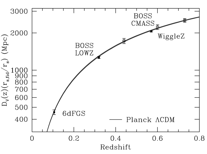
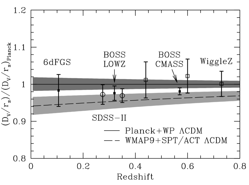
| dataset | ||||||
|---|---|---|---|---|---|---|
| Planck | 0.32 | |||||
| WMAP | 0.32 | |||||
| eWMAP | 0.32 | |||||
| LOWZ | 0.32 | - | - | - | ||
| Planck | 0.57 | |||||
| WMAP | 0.57 | |||||
| eWMAP | 0.57 | |||||
| CMASS-iso | 0.57 | - | - | - | ||
| CMASS | 0.57 |
Results from the BAO method have improved substantially in the last decade and we have now achieved measurements at a wide range of redshifts. In Fig. 21 we plot the distance-redshift relation obtained from isotropic acoustic scale fits in the latest galaxy surveys. In addition to the values from this paper, we include the acoustic scale measurement from the 6dFGS (Beutler et al., 2011) and WiggleZ survey (Blake et al., 2011; Kazin et al., 2014). As the BAO method actually measures , we plot this quantity multiplied by . The very narrow grey band here is the prediction from the Planck CMB dataset detailed in Sec. 9.1. In vanilla flat CDM, the CMB acoustic peaks imply precise measurements of and , which in turn imply the acoustic scale. The angular acoustic scale in the CMB then determines the distance to , which breaks the degeneracy between and once the low-redshift expansion history is otherwise specified (e.g., given , , and ). The comparison between low-redshift BAO measurements and the predictions from the CMB assuming a flat CDM cosmology therefore allows percent-level checks on the expansion history in this model over a large lever arm in redshift. One sees remarkably good agreement between the BAO measurements and the flat CDM predictions from CMB observations.
Fig. 22 divides by the best-fit prediction from Planck Collaboration (2013b) to allow one to focus on a percent-level comparison. In addition to the BAO data from the previous figure, we also plot older BAO measurements based primarily on SDSS-II LRG data (Percival et al., 2010; Padmanabhan et al., 2012). This figure also shows the flat CDM prediction from the WMAP+SPT/ACT data set. The predictions from these two data sets are in mild conflict due to the per cent difference in their values, discussed in Section 9.1. One can see that the isotropic BAO data, and the BOSS measurements in particular, fall between the two predictions and are consistent with both. Note that the recent revision of Planck data by Spergel et al. (2013) results in a value of that is in excellent agreement with our isotropic BAO measurements, which brings Planck predictions of the distance scale at and much closer to BOSS measurements.
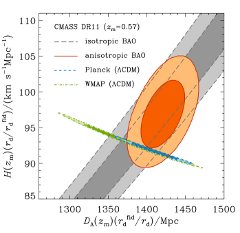
Our 68 and 95 per cent constraints in the plane from CMASS consensus anisotropic measurements are highlighted in orange in Fig. 23. In grey we overplot one-dimensional 1- and contours of our consensus isotropic BAO fit. Also shown in Fig. 23 are the flat CDM predictions from the Planck and WMAP CMB data sets detailed in Section 9.1. The CMB constraints occupy a narrow ellipse defined by the extremely precise measurement of the angular acoustic scale of 0.06 per cent (Planck Collaboration, 2013b). The extent of the ellipse arises primarily from the remaining uncertainty on the physical cold dark matter density, ; Planck narrows the allowed range by nearly a factor of two compared with WMAP. The CMASS isotropic BAO constraints are consistent with both CMB predictions shown here. The anisotropic constraints in particular prefer larger values of (right edge of the WMAP contour) also favored by Planck. Also evident in this plot is the offset between the best fit anisotropic constraint on (or ) and the flat CDM predictions from the CMB.
To make the flat CDM comparison between the CMB and our BAO measurements more quantitative, we report in Table LABEL:tab:CMBpredictions the Planck, WMAP, and eWMAP CDM predictions for our isotropic and anistropic BAO observables at and . All three predictions are in good agreement with our isotropic measurements. The largest discrepancy between the Planck CDM predictions and BOSS measurements is about for the anisotropic parameter (or the closely related ) at . eWMAP and BOSS disagree at about in , which leads to an approximately offset in .
Our measurements therefore provide no indication that additional parameters are needed to describe the expansion history beyond those in flat CDM. However, it is also clear from Fig. 22 and Table LABEL:tab:CMBpredictions that the disagreement between the WMAP+SPT/ACT and Planck CDM BAO predictions is comparable to the error on the BOSS acoustic scale measurement. Under the assumption of a flat CDM model, our anisotropic measurements show a mild preference for the Planck parameter space over WMAP+SPT/ACT. We are optimistic that the further analysis of the CMB data sets will resolve the apparent difference.
Since the uncertainties in the CDM prediction of the BAO observables from the CMB are dominated by the uncertainty in , another way to summarize and compare the BAO measurements across redshift is as a constraint on from the flat CDM model holding the CMB acoustic scale, (Eq. 10 of Planck Collaboration, 2013b), and physical baryon density, fixed. These values are given in the column of Table LABEL:tab:CMBpredictions. We stress that these inferences depend critically on the assumption of a flat CDM expansion history. Using this method, the BOSS inferences are more precise than the CMB and fall between the WMAP and Planck constraints. The isotropic CMASS analysis yields , in close agreement with the LOWZ result of . Our anisotropic analysis shifts to a notably larger value, , closer to the Planck measurement. This shift in between the isotropic and anisotropic CMASS fits is simply a restatement of the half sigma shift in between our isotropic and anistropic fits, discussed in Sec. 7.5.
For our cosmological parameter estimation, we present Planck in most cases but show the results for WMAP and WMAP+SPT/ACT in some cases so that the reader can assess the differences. For most combinations, the agreement is good. This is because the BAO data fall between the two CMB results and hence tend to pull towards reconciliation, and because the low-redshift data sets dominate the measurements of dark energy in cosmologies more complicated than the vanilla flat CDM model.
Fig. 23 and Table LABEL:tab:CMBpredictions illustrate many of the features of the CDM model fits we present in Table 14. For instance, the addition of a CMASS BAO measurement to the CMB improves the constraint on by 40 per cent for Planck (with similar improvements for the other CMB choices). The central values for all three reported CDM parameters shift by one sigma between isotropic and anisotropic CMASS fits. There are also one sigma shifts between Planck and WMAP/eWMAP central parameter values at fixed BAO measurements; taken together, WMAP+CMASS-iso or eWMAP+CMASS-iso and Planck+CMASS differ in their central values of and by about . Additionally combining with other BAO and SN measurements relaxes this tension to about . Within the context of the CDM model, the combination of CMB and BAO provides 1 per cent (3 per cent) constraints on and , respectively. These constraints relax by a factor of 3 (2) in the most general expansion history model, oCDM.
In Anderson et al. (2012) we showed that the BAO distance-redshift relation is consistent with that measured by Type Ia supernovae. This remains true with these DR11 results.
9.3 Cosmological parameter estimates in extended models
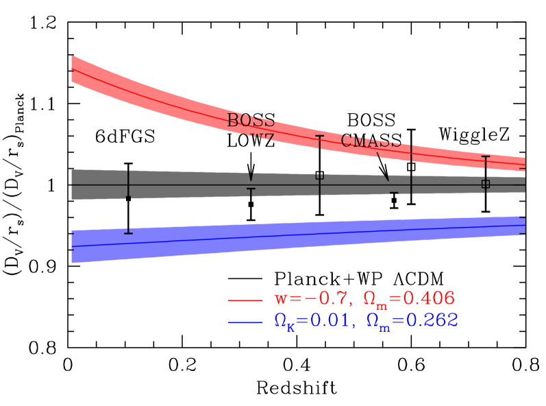
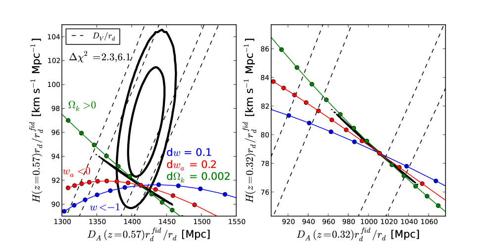
While the flat CDM expansion history is sufficient to explain current CMB and BAO measurements, the addition of precise low-redshift BAO distances greatly improves constraints on parameters that generalize the flat CDM expansion history. In this section we allow for non-zero spatial curvature (), a fixed equation of state for dark energy (), and a time-varying dark energy equation of state ( and ).
Fig. 24 illustrates the utility of BAO measurements for constraining these additional parameters. As one changes the model of the spatial curvature or dark energy equation of state, the and values required to simultaneously match the CMB measurement of and the distance to change. Here, we show the result assuming for a flat cosmology, as well as that for a closed Universe with and a cosmological constant. One can see that these predictions are sharply different from flat CDM at low redshift.
In Fig. 25 we focus instead on the two effective redshifts of our BAO observables, now examining how variations in the new parameters alter predictions for both and . For ease of comparison, we plot contours for both the isotropic (dashed) and anistropic (solid) fits; these values correspond to 68 and 95 per cent confidence regions when fitting two parameters. The extremely narrow black ellipse (nearly parallel with the green curve) shows the predictions from Planck in a flat CDM model; the uncertainty in the Planck predictions are dominated by the uncertainty in cold dark matter density, . The three colored curves cross at the Planck best fit cosmology, and show how the predictions for the BAO observables depend on each of the extra parameters. To produce these curves, we held , , and the CMB acoustic scale fixed; the reader should keep in mind that marginalizing over (the width of the Planck flat CDM prediction) will allow a larger range of parameter values to be consistent with both the CMB and BAO observables compared with the fixed case.
Fig. 25 already anticipates many of the results from detailed joint parameter fitting reported in Tables 14 and 15. For instance, by comparing the model variations to the isotropic BAO measurement uncertainties, the constraint on should be about 30 per cent better from the isotropic BAO feature than the measurement. For the case combining CMASS isotropic and Planck constraints, the uncertainty on (e.g., the extent of the flat CDM Planck contour) degrades the constraint on from to 0.003. For the wCDM model, the situation is reversed: the lower redshift isotropic BAO measurement is more constraining even though the fractional measurement errors are larger. The wCDM model curves also help explain why the Planck + CMASS-iso constraint, , does not improve the error on over our DR9 result, (Anderson et al., 2012), even though our error on the BAO scale has improved from 1.7 per cent to 1 per cent: models with , favored by our CMASS isotropic BAO measurement, produce smaller changes in the BAO observables at per unit change in than models close to . Moreover, the best-fit parameters for both the CMB and BAO datasets have shifted between DR9 and DR11. In fact, combining CMASS-DR9 with Planck instead of WMAP7 yields . In that case, the BAO and CMB flat CDM constraints have closer best fit values.
The left panel of Fig. 25 also demonstrates why the CMASS anisotropic constraints are more constraining than the isotropic ones, particularly for dark energy parameters. Variation in at fixed CMB acoustic scale primarily shifts , and the anisotropic measurements provide tighter constraints in that direction. Note that none of these extra parameters drive the expansion rate as high as our anisotropic best fit to .
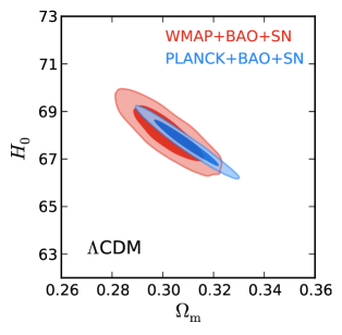
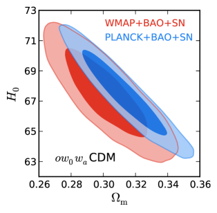
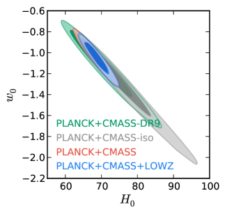
In order to explore our results on the full multi-dimensional parameter space in which we derive our cosmological constraints, we now describe the results of our MCMC chains. Here we use our BAO measurements in combination with CMB results, and supplemented at times by SN data and other BAO measurements, doing the analysis in the context of different cosmological models. We first start by comparing constraints on the parameters , , and from our different BAO datasets in Table 14. In this case we combine BAO with different CMB datasets: Planck, WMAP9, or eWMAP, in the CDM, oCDM, or wCDM cosmological models. We find that all CMB+BAO combinations return similar cosmological fits in CDM and oCDM models, with around 68 km s-1 Mpc-1, around 0.30, and negligible spatial curvature. Somewhat more variation is seen in the wCDM case, because of a degeneracy between and that is described later in this section. However, these variations are accompanied by larger formal errors and are highly consistent with the CDM fit. In our best constrained case (Planck+CMASS in CDM), we find a 1 per cent measurement of , a 1 per cent measurement of , and a 3 per cent measurement of . These broaden only slightly in oCDM, to 2 per cent in . We find a tight measurement of curvature, consistent with a flat Universe with 0.003 error.
The degeneracy between and is shown in Fig. 26. Here we compare the allowed parameter space in the case of Planck and WMAP9, for the minimal CDM model (left panel) and the oCDM model (Chevallier & Polarski, 2001; Linder, 2003) (right panel) The latter was recommended by the Dark Energy Task Force (hereafter DETF; Albrecht et al. 2006) for dark energy Figure of Merit comparisons. This model contains three more degrees of freedom (curvature and a time-dependent equation of state for dark energy). As was discussed in Mehta et al. (2012) and Anderson et al. (2012), the combination of CMB, BAO, and SNe data results produces a reverse distance ladder that results in tight constraints on and despite this flexibility in the cosmological model. The CMB determines the acoustic scale, which the BAO uses to measure the distance to intermediate redshift. The SNe then transfer that distance standard to low redshift, which implies . Combining this with the CMB measurement of yields . As shown in the figure, changing between Planck and WMAP data does not significantly shift these constraints.
As has been discussed before (Mehta et al., 2012; Anderson et al., 2012; Planck Collaboration, 2013b), the value inferred from this reverse distance ladder, km s-1 Mpc-1, is notably lower than some recent local measurements. For example, Riess et al. (2011) finds km s-1 Mpc-1 and Freedman et al. (2012) finds km s-1 Mpc-1. The Riess et al. (2011) value would be decreased by a small recalibration of the water maser distance to NGC 4258 (Humphreys et al., 2013). Efstathiou (2013) warns about possible biases in the period-luminosity relation fits due to low-metallicity Cepheids and finds a lower value of km s-1 Mpc-1 using only NGC 4258 as the primary distance standard, including the maser recalibration, or km s-1 Mpc-1 using three sets of primary standards. While we believe that the comparison of these direct measurements to our BAO results is important, the results are also affected by the ongoing photometric recalibration of the SDSS and SNLS SNe data (Betoule et al., 2013). We have therefore not pursued a more quantitative assessment at this time.
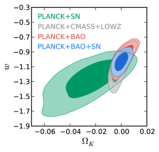
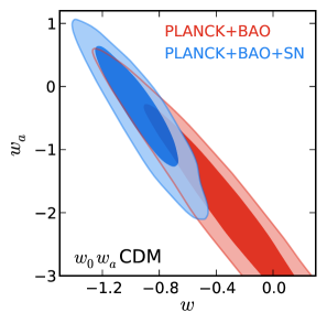
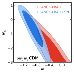
We next discuss how BAO can help constrain additional degrees of freedom. In Table 15 we present our results in more general cosmological models: CDM, oCDM (adding curvature), CDM (adding a equation of state parameter for dark energy), oCDM (adding both), CDM (allowing for time-dependence in the e.o.s. of dark energy), and oCDM (our most general model, for DETF comparisons). In each case, we begin with the results of combining our CMASS and LOWZ data with Planck, showing both isotropic and anisotropic CMASS cases. We then extend the data combination with anisotropic CMASS to include additional BAO information from the 6dFGS and Ly forest, as well as SNe results from the Union 2 compilation. Finally, for the full combination of BAO and SNe, we vary the CMB measurements between Planck, WMAP, and eWMAP to explore any dependency on the tensions between those data sets.
We find that these datasets can constrain the equation of state of dark energy to 6 per cent and curvature to 0.2 per cent, although the time evolution of dark energy is still unconstrained. In the DETF cosmology, we find a Figure of Merit value (inverse square root of the minor of the covariance matrix containing the covariances of and ) of 13.5. We find that the anisotropic BAO measurement from CMASS-DR11 is much more powerful when constraining the equation of state of dark energy (even when considering time-evolving dark energy) than its isotropic counterpart.
Fig. 27 shows the constraints in the – plane for different BAO datasets combined with Planck results. The degeneracy between both parameters is quite evident, showing that a more negative value for can result in a higher estimation for the Hubble constant. This effect can also be seen in Fig. 24; for the CDM model, variations in the distance to intermediate redshift produce larger variations in the local distance scale. The extent of the error contours as we vary the choice BAO data set is somewhat complicated, as was illustrated in Fig. 25. The efficacy of a given BAO distance precision to constrain degrades as the fit shifts to more negative values of ; this is because models with have their dark energy disappear by intermediate redshift, leaving the BAO and CMB constraints degenerate. The improvement when we change from the isotropic CMASS results to the anisotropic ones is partially due to a shift in toward 0 and partially because of the rotation of the contours to favor a constraint. Overall, this figure also shows the consistency between the various BOSS results and the tight constraints on that the BAO now provides.
We turn next to the oCDM case, attempting to measure a constant dark energy equation of state in the presence of non-zero spatial curvature. These constraints are shown in Fig. 28 for several combinations of datasets. The allowed region in this parameter space by the combination CMB+SN is large, due to a substantial degeneracy between and curvature. This degeneracy is lifted by the BAO, which in combination with the CMB sharply constrains the curvature. Even without the SNe data, the BAO distance constraints are now strong enough to measure while simultaneously measuring . With Planck, CMASS, and LOWZ measurements alone, we find . Further combine with the BAO measurement from 6dF and the Lyman-alpha forest BAO measurement from BOSS, we find . In both cases, the fitted cosmologies are consistent with a flat Universe. Hence, the BAO distance scale now provides enough precision, without additional data beyond the CMB, to measure to 11 per cent even while marginalizing over spatial curvature. It is remarkable that the BAO data prefers a flat Universe with despite simultaneously opening two additional degrees of freedom relative to the flat cosmological constant model. We note the BAO and SNe constraints remain highly complementary in their degeneracy directions; adding the SN data shrinks the allowed region further, to while remaining consistent with a flat Universe.
Finally, in Fig. 29 we show our constraints on a time-dependent dark energy equation of state. The contours show the allowed parameter space using the combination of CMB and BAO data, with and without SNe data, in a flat CDM model (left panel) and an oCDM model with curvature (right panel). This parameter space is poorly constrained, with a clear degeneracy between the and parameters, such that less negative values of are related to more negative values of . The addition of SN data suppress the likelihood of less negative values, greatly reducing the allowed parameter space. We note that allowing non-zero spatial curvature degrades the dark energy constraints, but not catastrophically. The area covered by the 2– contour in the CDM case is the DETF Figure of Merit.
10 Conclusion
We have presented constraints on cosmology and the distance-redshift relation from the Data Release 10 and 11 galaxy samples of the Baryon Oscillation Spectroscopic sample. These results, based on the largest volume of the Universe ever surveyed at this high density (, including both LOWZ and CMASS samples), provide the strongest constraints on the distance-redshift relation achieved with the BAO method and the most accurate determination of the distance scale in the crucial redshift range where the expansion of the Universe begins to accelerate.
The combination of large survey volume, high sampling density and high bias of the LOWZ and CMASS galaxies allows detection of the acoustic oscillation signal at unprecedented significance. The acoustic signature is seen in both the power spectrum and the correlation function, before density field reconstruction and after reconstruction. The measures are all highly consistent and the values and errors are in accord with our models and mock catalogs (Manera et al., 2013a, 2014). Unlike our earlier results based upon DR9, we find density-field reconstruction significantly improves our measurement of the acoustic scale (see Fig. 4), with the amount of improvement consistent with expectations if the underlying cosmology were of the CDM family.
With the larger volume of data, we now have statistically significant evidence for variations in the target catalog density that are correlated with seeing and stellar density. We correct for these systematics, along with a correction for redshift failures and galaxies for which a redshift was not obtained due to fiber collisions, using weights. A similar procedure was used in Anderson et al. (2012), except the weights have been revised to correct for the effects of seeing.
We fit the acoustic signature to an appropriately scaled template in both the correlation function and power spectrum, marginalizing over broad-band shape. Our results are insensitive to the model of broad-band power and highly consistent between configuration- and Fourier-space. As an extension of the work reported in Anderson et al. (2012), we now explicitly consider the effects of binning in the correlation function and power spectrum and combine the two methods using several different binning choices. We measure a spherically averaged distance, , in units of the sound-horizon, , at two “effective” redshifts: and . Our consensus results for the distance, including a budget for systematic errors, are and . The measurement at is the first ever 1 per cent measurement of a distance using the BAO method.
As in Anderson et al. (2014), we have used the anisotropy in the measured configuration-space clustering, induced by redshift-space distortions, to separately constrain the distance along and across the line-of-sight. We compress the dependence on the angle to the line-of-sight into two statistics, either the multipole moments or “wedges”. We obtain consistent fits from both methods. A detailed study of possible systematics in inferences from anisotropic clustering is presented in Vargas-Magana et al. (2013). Our consensus results for the CMASS sample at are and with a correlation coefficient between the two of .
Samushia et al. (2014), Beutler et al. (2013) and Sánchez et al. (2013b) have used the correlation function and power spectrum over a wide range of scales, along with a model for the broad-band power, to constrain cosmological parameters including the distance-redshift relation and . We find excellent agreement between their results and the pure-BAO measurement described here, despite differences in the procedure. This is not unexpected, in that the bulk of the information is contained in the acoustic signal rather than the broad-band power.
The BOSS results provide the tightest constraints in an reverse distance ladder that tightly constrains the expansion rate from to . The measurements reported here are in excellent agreement with earlier BAO results by BOSS Anderson et al. (2012) and by other groups (Percival et al., 2010; Beutler et al., 2011; Blake et al., 2011; Padmanabhan et al., 2012).
The DR11 distance to is approximately per cent smaller than that reported to the same redshift based on the DR9 data. This shift is approximately relative to the DR9 error bars. As the data set has tripled in size, such a shift is consistent with expectations. Both the and distance measurements are highly consistent with expectations from the Planck and WMAP CMB measurements assuming a CDM model, lying approximately midway between the inferences from the two experiments. Our results for and are similarly consistent with both CMB data sets; in detail, the anisotropic results are slightly closer to the Planck best fit CDM prediction. While there are some mild tensions between the CMB data sets, the distance scale inferred from acoustic oscillations in the distant Universe () and in the local Universe () are in excellent agreement with the predictions of a CDM model, with gravity well described by General Relativity and with a time-independent and spatially constant dark energy with equation-of-state .
The BOSS will finish data taking within the next year. Along with the additional data, constraints at higher from the Ly forest, improvements in the analysis and a full systematic error study, we expect BOSS to provide the definitive measurement of the absolute distance scale out to for some time to come.
11 Acknowledgements
Funding for SDSS-III has been provided by the Alfred P. Sloan Foundation, the Participating Institutions, the National Science Foundation, and the U.S. Department of Energy Office of Science. The SDSS-III web site is http://www.sdss3.org/.
SDSS-III is managed by the Astrophysical Research Consortium for the Participating Institutions of the SDSS-III Collaboration including the University of Arizona, the Brazilian Participation Group, Brookhaven National Laboratory, University of Cambridge, Carnegie Mellon University, University of Florida, the French Participation Group, the German Participation Group, Harvard University, the Instituto de Astrofisica de Canarias, the Michigan State/Notre Dame/JINA Participation Group, Johns Hopkins University, Lawrence Berkeley National Laboratory, Max Planck Institute for Astrophysics, Max Planck Institute for Extraterrestrial Physics, New Mexico State University, New York University, Ohio State University, Pennsylvania State University, University of Portsmouth, Princeton University, the Spanish Participation Group, University of Tokyo, University of Utah, Vanderbilt University, University of Virginia, University of Washington, and Yale University.
We acknowledge the use of the Legacy Archive for Microwave Background Data Analysis (LAMBDA). Support for LAMBDA is provided by the NASA Office of Space Science.
This research used resources of the National Energy Research Scientific Computing Center, which is supported by the Office of Science of the U.S. Department of Energy under Contract No. DE-AC02-05CH11231.
Some of the CMASS reconstruction and MCMC computations were supported by facilities and staff of the Yale University Faculty of Arts and Sciences High Performance Computing Center.
LOWZ reconstruction computations were supported by the facilities and staff of the UK Sciama High Performance Computing cluster supported by SEPNet and the University of Portsmouth. Power spectrum calculations, and fitting made use of the COSMOS/Universe supercomputer, a UK-CCC facility supported by HEFCE and STFC in cooperation with CGI/Intel.
We thank Christian Reichardt for his help in using the actlite likelihood code.
References
- Abazajian et al. (2004) Abazajian, K., et al. 2004, AJ, 128, 502
- Abazajian et al. (2009) Abazajian, K. N., et al., 2009, ApJS, 182, 543 (DR7)
- Planck Collaboration (2013a) Ade et al., Planck Collaboration I, 2013a, arXiv1303.5062
- Planck Collaboration (2013b) Ade et al., Planck Collaboration XVI, 2013b, arXiv1303.5076
- Ahn et al. (2013) Ahn C., et al., 2013, AJ, submitted, arxiv:1307.7735
- Aihara et al. (2011) Aihara H., et al., 2011, ApJS, 193, 29
- Alcock & Paczynski (1979) Alcock C., Paczynski B., 1979, Nature, 281, 358.
- Albrecht et al. (2006) Albrecht A., et al., 2006, arXiv:astro-ph/0609591
- Anderson et al. (2012) Anderson L., et al., 2012, MNRAS, 427, 3435
- Anderson et al. (2014) Anderson L., et al., 2014, MNRAS, 439, 83
- Bennett et al. (2013) Bennett, C., et al., 2013, ApJS, 208, 20
- Bernardeau et al. (2002) Bernardeau F., Colombi S., Gaztanaga E., Scoccimarro R., Physics Reports, 367, 1
- Betoule et al. (2013) Betoule, M., et al., 2013, A&A, 552, 124
- Beutler et al. (2011) Beutler F., et al., 2011, MNRAS, 416, 3017
- Beutler et al. (2013) Beutler F., et al., 2013, arXiv:1312.4611
- Blake et al. (2011) Blake C., et al., 2011, MNRAS, 415, 1707
- Blanton et al. (2003) Blanton M., et al., 2003, AJ, 125, 2276
- Bolton et al. (2012) Bolton A., et al., 2012, AJ, 144, 144
- Busca et al., (2013) Busca, N.G., et al., 2013, A&A, 552, 96
- Calabrese et al., (2013) Calabrese, E. et al., 2013, Phys. Rev. D, 87, 103012
- Carnero et al. (2012) Carnero, A., et al., 2012, MNRAS, 419, 1689
- Chevallier & Polarski (2001) Chevallier M., Polarski D., 2001, Int. J. Mod. Phys. D 10, 213
- Chuang & Wang (2011) Chuang, C.-H., Wang, Y., 2011, MNRAS, 426, 226
- Chuang et al. (2013) Chuang, C.-H., et al., 2013, MNRAS, 433, 3559
- Chuang et al. (2013b) Chuang, C.-H., et al., 2013b,
- Cole et al. (2005) Cole S., et al., 2005, MNRAS, 362, 505
- Colless et al. (2003) Colless M., et al., 2003, [astro-ph/0306581]
- Crocce & Scoccimarro (2006) Crocce, M., & Scoccimarro, R., 2006, Phys. Rev. D, 73,
- Crocce & Scoccimarro (2008) Crocce, M., & Scoccimarro, R., 2008, Phys. Rev. D, 77, 023533
- Das et al. (2013) Das, S., et al. 2013, arXiv:1301.1037
- Dawson et al. (2012) Dawson K., et al., 2012, AJ, 145, 10
- Doi et al. (2010) Doi M., et al., 2010, AJ, 139, 1628
- Doroshkevich et al. (1978) Doroshkevich A.G., Zel’dovich Ya.B., Sunyaev R.A., 1978 Soviet Astronomy, 22, 523
- Dunkley et al. (2013) Dunkley J., et al., 2013, JCAP, 07, 025
- Efstathiou (2013) Efstathiou, G., 2013, arXiv:1311.3461
- Eisenstein & Hu (1998) Eisenstein D.J., Hu W., 1998, ApJ, 496, 605
- Eisenstein et al. (2005) Eisenstein D.J., et al., 2005, ApJ, 633, 560
- Eisenstein, Seo & White (2006) Eisenstein D.J., Seo H.J., White, M., 2006, ApJ, 664, 660
- Eisenstein et al. (2007a) Eisenstein D. J., Seo H.-J., Sirko E., Spergel D. N., 2007a, ApJ, 664, 675
- Eisenstein et al. (2007b) Eisenstein D.J., Seo H.-J., White M., 2007b, ApJ, 664, 660
- Eisenstein et al. (2011) Eisenstein D.J., et al., 2011, AJ, 142, 72 [arxiv:1101.1529]
- Feldman, Kaiser & Peacock (1994) Feldman H.A., Kaiser N., Peacock J.A., 1994, ApJ, 426, 23
- Font-Ribera et al. (2013) Font-Ribera A., et al., 2013, preprint [arxiv:1311.1767]
- Forero, Tórtola, & Valle (2012) Forero D.V., Tórtola M., Valle J., Phys. Rev. D86, 073012
- Freedman et al. (2012) Freedman, W. L., et al., 2012, ApJ, 758, 24
- Fukugita et al. (1996) Fukugita M., et al., 1996, AJ, 111, 1748
- Gaztanaga, Cabre & Hui (2009) Gaztanaga E., Cabre A., Hui L., 2009, MNRAS, 399, 1663
- Goroff et al. (1986) Goroff M.H., Grinstein B., Rey S.-J., Wise M.B., 1986, ApJ, 311, 6
- Górski et al. (2005) Górski, K. M., Hivon, E., Banday, A. J., Wandelt, B. D., Hansen, F. K., Reinecke, M., Bartelmann, M. 2005, ApJ, 622, 759
- Gunn et al. (1998) Gunn J.E., et al., 1998, AJ, 116, 3040
- Gunn et al. (2006) Gunn J.E., et al., 2006, AJ, 131, 2332
- Hamilton & Tegmark (2000) Hamilton, A.J.S., Tegmark, M., 2000, MNRAS, 312, 285
- Ho et al. (2012) Ho, S., et al., 2012, ApJ, 761, 14
- Høg et al. (2000) Høg, E., et al., 2000, A&A, 355, 27
- Humphreys et al. (2013) Humphreys, L., et al., 2013, 775, 13
- Hutsi (2006) Hütsi G., 2006, A&A, 449, 891
- Jain & Bertschinger (1994) Jain B., Bertschinger E., 1994, ApJ, 431, 495.
- Kaiser (1987) Kaiser N., 1987, MNRAS, 227, 1
- Kazin et al. (2012) Kazin E., Sanchez A.G., Blanton M.R., 2012, MNRAS, 419, 3223
- Kazin et al. (2013) Kazin E., et al., 2013, MNRAS, 435, 64
- Kazin et al. (2014) Kazin E.A., Koda, J., Blake, C., Padmanabhan, N., MNRAS, submitted, arXiv:1401.0358
- Kirkby et al. (2013) Kirkby, D., et al., 2013, JCAP, 3, 24
- Landy & Szalay (1993) Landy S.D., Szalay A.S., 1993, ApJ 412, 64
- Lewis et al. (2000) Lewis A., Challinor A., Lasenby A., 2000, ApJ, 538, 473
- Lewis & Bridle (2002) Lewis A., Bridle S., 2002, PhRvD, 66, 103511
- Linder (2003) Linder E. V., 2003, PhRvD, 90, 091301
- Lupton et al. (2001) Lupton R., Gunn J.E., Ivezić Z., Knapp G., Kent S., 2001, “Astronomical Data Analysis Software and Systems X”, v.238, 269.
- Makino, Sasaki & Suto (1992) Makino N., Sasaki M., Suto Y., 1992, Phys. Rev. D46, 585.
- Manera et al. (2013a) Manera, M., et al. 2013, MNRAS, 428, 1036
- Manera et al. (2014) Manera, M., et al., 2014, arXiv:1401.4171
- Maraston et al. (2013) Maraston, C., et al. 2013, MNRAS, 435, 2764
- Matsubara (2008b) Matsubara T., 2008b, Phys. Rev. D, 77, 063530
- McQuinn & O’Leary (2012) McQuinn M., O’Leary R.M., 2012, ApJ, 760, 3
- Mehta et al. (2011) Mehta K. T., Seo H.-J., Eckel J., Eisenstein D. J., Metchnik M., Pinto P., Xu X., 2011, ApJ, 734, 94
- Mehta et al. (2012) Mehta K., et al., 2012, MNRAS, 427, 2168
- Meiksin, White & Peacock (1999) Meiksin A., White M., Peacock J.A., 1999, MNRAS 304, 851
- Mortonson, Weinberg & White (2014) Mortonson M.J., Weinberg D.H., White M., 2014, Particle Data Group 2014 Review of Particle Physics, Chapter 25. [arxiv:1401.0046]
- Noh, White & Padmanabhan (2009) Noh Y., White M., Padmanabhan N., 2009, Phys. Rev. D, 80, 123501
- Nuza et al. (2013) Nuza S.E., et al., 2013, MNRAS, 432, 743
- Okumura et al. (2008) Okumura T., et al., 2008, ApJ, 676, 889
- Padmanabhan et al. (2007) Padmanabhan N., et al., 2007, MNRAS, 378, 852
- Padmanabhan et al. (2008) Padmanabhan N., et al., 2008, ApJ, 674, 1217
- Padmanabhan & White (2009) Padmanabhan N., White M., 2009, Phys. Rev. D, 80, 063508
- Padmanabhan et al. (2012) Padmanabhan N., Xu X., Eisenstein D.J., Scalzo R., Cuesta A.J., Mehta K.T., Kazin E., 2012, MNRAS, 427, 2132
- Parejko et al. (2013) Parejko, J. K., Sunayama, T., Padmanabhan, N., et al. 2013, MNRAS, 429, 98
- Peacock & Dodds (1994) Peacock J.A., Dodds S.J., 1994, MNRAS, 267, 1020
- Peebles & Yu (1970) Peebles P.J.E., Yu J.T., 1970, ApJ, 162, 815
- Percival et al. (2007) Percival W.J., et al., 2007, MNRAS, 381, 1053
- Percival et al. (2010) Percival W.J., et al., 2010, MNRAS, 401, 2148
- Percival et al. (2014) Percival W.J., et al., 2014, MNRAS, in press, arXiv:1312.4841
- Perlmutter et al. (1999) Perlmutter S. et al., 1999, ApJ, 517, 565
- Pier et al. (2003) Pier J.R., et al., 2003, AJ, 125, 1559
- Reichardt et al. (2012) Reichardt, C. L., et al. 2012, ApJ, 755, 70
- Reid et al. (2011) Reid B.A., et al., 2011, MNRAS, 417, 1913R
- Reid et al. (2012) Reid B.A., et al., 2012, MNRAS, 426, 2719
- Riess et al. (1998) Riess A. G. et al., 1998, AJ, 116, 1009
- Riess et al. (2011) Riess A. G., et al., 2011, ApJ, 730, 119
- Ross et al. (2011) Ross A. J., et al., 2011, MNRAS, 417, 1350
- Ross et al. (2012) Ross, A. J., Percival, W. J., Sánchez, A. G., et al. 2012, MNRAS, 424, 564
- Ross et al. (2014) Ross A. J., et al., 2014, MNRAS, 437, 1109
- Rybicki & Press (1995) Rybicki, G.B., Press, W.H., 1995, PRL, 74, 1060
- Samushia et al. (2014) Samushia L., et al., 2014, MNRAS, in press, arXiv:1312.4899
- Sánchez et al. (2013a) Sánchez, A. G., et al., 2013a, MNRAS, 433, 1201
- Sánchez et al. (2013b) Sánchez, A. G., et al., 2013b, arXiv:1312.4854
- Schlegel, Finkbeiner & Davis (1998) Schlegel D.J., Finkbeiner D.P., Davis M., 1998, ApJ, 500, 525
- Seo et al. (2008) Seo H.-J., Siegel, E. R., Eisenstein, D. J., White, M., 2008, ApJ, 686, 13
- Seo et al. (2010) Seo H.-J., et al., 2010, ApJ, 720, 1650
- Seo et al. (2012) Seo H.-J., et al., 2012, ApJ, 761, 13
- Slosar et al. (2013) Slosar, A., et al., 2013, JCAP, 4, 26
- Smee et al. (2013) Smee S., et al., 2013, AJ, 146, 32
- Smith et al. (2002) Smith J.A., et al., 2002, AJ, 123, 2121
- Spergel et al. (2013) Spergel D., Flauger R., Hlozek R., 2013, arXiv:1312.3313
- Story et al. (2013) Story K.T., et al., 2013, ApJ, 779, 86
- Stoughton et al. (2002) Stoughton C., et al., 2002, AJ, 123, 485
- Strauss et al. (2002) Strauss M.A., et al., 2002, AJ, 124, 1810
- Sunyaev & Zel’dovich (1970) Sunyaev R.A., Zel’dovich Ya.B., 1970, ApSS, 7, 3
- Suzuki et al. (2012) Suzuki N., et al., 2012, ApJ, 746, 24
- Swanson et al. (2008) Swanson M.E.C., Tegmark M., Hamilton A.J.S., Hill J.C., 2008, MNRAS, 387, 1391
- Taruya, Nishimichi & Saito (2010) Taruya A., Nishimichi, T., Saito, S., 2010, PhRvD, 82
- Tegmark et al. (2004) Tegmark M., et al., 2004, ApJ, 606, 702
- Tegmark et al. (2006) Tegmark M., et al., 2006, Phys. Rev. D, 74, 123507
- Thomas et al. (2013) Thomas D., et al., 2013, MNRAS, 431, 1383
- Tojeiro et al. (2012) Tojeiro, R., et al., 2012, MNRAS, 424, 136
- Tojeiro et al. (2014) Tojeiro R., et al., 2014, arXiv:1401.1768
- Tseliakhovich & Hirata (2010) Tseliakhovich, D., Hirata, C., 2010, Phys. Rev. D, 82, 083520
- Vargas-Magana et al. (2013) Vargas-Magana., et al., 2013, arXiv:1312.4996
- Veropalumbo et al. (2014) Veropalumbo A., Marulli F., Moscardini L., Moresco M., Cimatti A., 2014, MNRAS, submitted, arXiv:1311.5895
- Weinberg et al. (2013) Weinberg, D. H., Mortonson M.J., Eisenstein D.J., Hirata C., Reiss A.G., Rozo, E., 2013, Phys. Rep. 530, 87
- White et al. (2011) White M., et al., 2011, ApJ, 728, 126
- Xu et al. (2012a) Xu, X., et al., 2012a, MNRAS, 427, 2146
- Xu et al. (2012b) Xu, X., et al., 2012b, MNRAS, 431, 2834
- Yoo & Seljak (2013) Yoo, J., Seljak, U., 2013, PRD, 88, 103520
- York et al. (2000) York D.G., et al., 2000, AJ, 120, 1579
| Cosmological | Data Sets | |||||
| Model | km s-1 Mpc-1 | |||||
| CDM | Planck | 0.1427 (24) | 0.316 (16) | 67.3 (11) | ||
| CDM | WMAP | 0.1371 (44) | 0.284 (25) | 69.6 (21) | ||
| CDM | eWMAP | 0.1353 (35) | 0.267 (19) | 71.3 (17) | ||
| CDM | Planck + CMASS-DR9 | 0.1428 (20) | 0.317 (13) | 67.1 (9) | ||
| CDM | Planck + CMASS-iso | 0.1408 (15) | 0.304 (9) | 68.1 (7) | ||
| CDM | Planck + CMASS | 0.1418 (15) | 0.311 (9) | 67.6 (6) | ||
| CDM | Planck + LOWZ | 0.1416 (20) | 0.309 (13) | 67.7 (9) | ||
| CDM | WMAP + CMASS-DR9 | 0.1403 (30) | 0.305 (16) | 67.9 (12) | ||
| CDM | WMAP + CMASS-iso | 0.1383 (25) | 0.292 (10) | 68.8 (8) | ||
| CDM | WMAP + CMASS | 0.1400 (24) | 0.302 (10) | 68.0 (8) | ||
| CDM | WMAP + LOWZ | 0.1379 (30) | 0.289 (15) | 69.2 (13) | ||
| CDM | eWMAP + CMASS-DR9 | 0.1401 (25) | 0.295 (14) | 69.0 (11) | ||
| CDM | eWMAP + CMASS-iso | 0.1393 (18) | 0.290 (9) | 69.3 (7) | ||
| CDM | eWMAP + CMASS | 0.1409 (17) | 0.300 (9) | 68.6 (7) | ||
| CDM | eWMAP + LOWZ | 0.1409 (24) | 0.282 (13) | 69.9 (11) | ||
| oCDM | Planck + CMASS-DR9 | 0.1418 (25) | 0.323 (15) | 66.3 (14) | -0.0029 (42) | |
| oCDM | Planck + CMASS-iso | 0.1418 (25) | 0.303 (9) | 68.4 (8) | +0.0016 (30) | |
| oCDM | Planck + CMASS | 0.1420 (24) | 0.311 (9) | 67.5 (8) | +0.0000 (30) | |
| oCDM | Planck + LOWZ | 0.1418 (25) | 0.307 (14) | 68.0 (15) | +0.0007 (42) | |
| oCDM | WMAP + CMASS-DR9 | 0.1372 (41) | 0.306 (15) | 67.0 (14) | -0.0050 (48) | |
| oCDM | WMAP + CMASS-iso | 0.1370 (41) | 0.290 (11) | 68.7 (10) | -0.0017 (41) | |
| oCDM | WMAP + CMASS | 0.1378 (41) | 0.300 (10) | 67.8 (9) | -0.0027 (41) | |
| oCDM | WMAP + LOWZ | 0.1371 (41) | 0.291 (15) | 68.7 (16) | -0.0017 (50) | |
| oCDM | eWMAP + CMASS-DR9 | 0.1356 (35) | 0.302 (15) | 67.1 (14) | -0.0079 (44) | |
| oCDM | eWMAP + CMASS-iso | 0.1357 (36) | 0.288 (10) | 68.6 (9) | -0.0045 (37) | |
| oCDM | eWMAP + CMASS | 0.1360 (36) | 0.296 (9) | 67.7 (8) | -0.0061 (38) | |
| oCDM | eWMAP + LOWZ | 0.1357 (35) | 0.288 (15) | 68.6 (16) | -0.0046 (47) | |
| CDM | Planck + CMASS-DR9 | 0.1439 (23) | 0.284 (48) | 72.1 (71) | -1.19 (26) | |
| CDM | Planck + CMASS-iso | 0.1439 (23) | 0.251 (36) | 76.4 (66) | -1.33 (24) | |
| CDM | Planck + CMASS | 0.1425 (22) | 0.305 (20) | 68.5 (25) | -1.04 (11) | |
| CDM | Planck + LOWZ | 0.1432 (24) | 0.279 (26) | 72.0 (36) | -1.17 (14) | |
| CDM | WMAP + CMASS-DR9 | 0.1378 (50) | 0.324 (47) | 65.9 (65) | -0.91 (27) | |
| CDM | WMAP + CMASS-iso | 0.1380 (47) | 0.288 (37) | 69.9 (61) | -1.04 (26) | |
| CDM | WMAP + CMASS | 0.1354 (43) | 0.323 (18) | 64.8 (25) | -0.84 (12) | |
| CDM | WMAP + LOWZ | 0.1373 (47) | 0.292 (25) | 68.8 (36) | -0.99 (16) | |
| CDM | eWMAP + CMASS-DR9 | 0.1366 (35) | 0.341 (34) | 63.5 (36) | -0.79 (13) | |
| CDM | eWMAP + CMASS-iso | 0.1360 (35) | 0.311 (22) | 66.2 (30) | -0.87 (12) | |
| CDM | eWMAP + CMASS | 0.1354 (33) | 0.330 (16) | 64.1 (20) | -0.80 (8) | |
| CDM | eWMAP + LOWZ | 0.1358 (35) | 0.299 (23) | 67.5 (29) | -0.90 (10) |
| Cosmological | Data Sets | ||||||
| Model | km s-1 Mpc-1 | ||||||
| CDM | Planck + CMASS-iso + LOWZ | 0.1405 (14) | 0.302 (8) | 68.2 (6) | |||
| CDM | Planck + CMASS + LOWZ | 0.1415 (14) | 0.308 (8) | 67.8 (6) | |||
| CDM | Planck + BAO | 0.1417 (13) | 0.310 (8) | 67.6 (6) | |||
| CDM | Planck + CMASS + LOWZ + SN | 0.1414 (13) | 0.308 (8) | 67.8 (6) | |||
| CDM | Planck + BAO + SN | 0.1416 (13) | 0.309 (8) | 67.7 (6) | |||
| CDM | WMAP + BAO + SN | 0.1399 (22) | 0.302 (8) | 68.1 (7) | |||
| CDM | eWMAP + BAO + SN | 0.1411 (16) | 0.301 (8) | 68.5 (6) | |||
| oCDM | Planck + CMASS-iso + LOWZ | 0.1417 (25) | 0.302 (8) | 68.5 (8) | +0.0017 (30) | ||
| oCDM | Planck + CMASS + LOWZ | 0.1420 (25) | 0.309 (8) | 67.8 (7) | +0.0006 (30) | ||
| oCDM | Planck + BAO | 0.1423 (25) | 0.311 (8) | 67.7 (7) | +0.0007 (29) | ||
| oCDM | Planck + CMASS + LOWZ + SN | 0.1416 (24) | 0.308 (8) | 67.9 (7) | +0.0003 (30) | ||
| oCDM | Planck + BAO + SN | 0.1419 (24) | 0.309 (8) | 67.7 (7) | +0.0004 (29) | ||
| oCDM | WMAP + BAO + SN | 0.1384 (40) | 0.300 (9) | 67.9 (8) | -0.0019 (40) | ||
| oCDM | eWMAP + BAO + SN | 0.1364 (34) | 0.296 (8) | 67.9 (7) | -0.0054 (35) | ||
| CDM | Planck + CMASS-iso + LOWZ | 0.1431 (22) | 0.274 (21) | 72.5 (32) | -1.19 (13) | ||
| CDM | Planck + CMASS + LOWZ | 0.1425 (21) | 0.299 (16) | 69.1 (21) | -1.07 (9) | ||
| CDM | Planck + BAO | 0.1419 (21) | 0.308 (14) | 67.9 (18) | -1.01 (8) | ||
| CDM | Planck + CMASS + LOWZ + SN | 0.1426 (19) | 0.299 (12) | 69.1 (16) | -1.07 (7) | ||
| CDM | Planck + BAO + SN | 0.1423 (19) | 0.305 (12) | 68.4 (14) | -1.04 (6) | ||
| CDM | WMAP + BAO + SN | 0.1380 (33) | 0.307 (12) | 67.0 (16) | -0.94 (8) | ||
| CDM | eWMAP + BAO + SN | 0.1379 (28) | 0.312 (11) | 66.5 (15) | -0.90 (7) | ||
| oCDM | Planck + CMASS-iso + LOWZ | 0.1418 (25) | 0.261 (31) | 74.1 (46) | -0.0022 (36) | -1.27 (21) | |
| oCDM | Planck + CMASS + LOWZ | 0.1420 (24) | 0.298 (23) | 69.2 (27) | -0.0005 (44) | -1.08 (14) | |
| oCDM | Planck + BAO | 0.1422 (24) | 0.315 (19) | 67.3 (20) | +0.0018 (44) | -0.98 (11) | |
| oCDM | Planck + CMASS + LOWZ + SN | 0.1421 (25) | 0.298 (14) | 69.1 (16) | -0.0008 (34) | -1.07 (8) | |
| oCDM | Planck + BAO + SN | 0.1422 (25) | 0.306 (13) | 68.2 (15) | +0.0002 (34) | -1.03 (7) | |
| oCDM | WMAP + BAO + SN | 0.1374 (42) | 0.306 (13) | 67.1 (16) | -0.0010 (44) | -0.95 (8) | |
| oCDM | eWMAP + BAO + SN | 0.1357 (35) | 0.305 (13) | 66.7 (15) | -0.0039 (40) | -0.93 (8) | |
| CDM | Planck + CMASS-iso + LOWZ | 0.1434 (22) | 0.302 (53) | 69.8 (66) | -0.90 (51) | -0.78 (124) | |
| CDM | Planck + CMASS + LOWZ | 0.1431 (21) | 0.350 (41) | 64.3 (41) | -0.54 (39) | -1.41 (101) | |
| CDM | Planck + BAO | 0.1428 (21) | 0.361 (32) | 63.1 (29) | -0.43 (30) | -1.62 (84) | |
| CDM | Planck + CMASS + LOWZ + SN | 0.1433 (22) | 0.304 (17) | 68.7 (19) | -0.98 (19) | -0.36 (64) | |
| CDM | Planck + BAO + SN | 0.1431 (22) | 0.311 (16) | 67.8 (18) | -0.93 (18) | -0.41 (62) | |
| CDM | WMAP + BAO + SN | 0.1372 (43) | 0.302 (16) | 67.5 (17) | -1.00 (16) | 0.16 (59) | |
| CDM | eWMAP + BAO + SN | 0.1366 (31) | 0.300 (15) | 67.5 (17) | -1.04 (14) | 0.41 (40) | |
| oCDM | Planck + CMASS-iso + LOWZ | 0.1419 (25) | 0.296 (50) | 70.0 (62) | -0.0042 (40) | -0.83 (45) | -1.41 (115) |
| oCDM | Planck + CMASS + LOWZ | 0.1417 (25) | 0.347 (38) | 64.2 (37) | -0.0039 (47) | -0.50 (34) | -1.79 (91) |
| oCDM | Planck + BAO | 0.1420 (24) | 0.361 (30) | 62.9 (27) | -0.0020 (47) | -0.40 (28) | -1.82 (82) |
| oCDM | Planck + CMASS + LOWZ + SN | 0.1419 (25) | 0.306 (16) | 68.1 (19) | -0.0042 (44) | -0.87 (20) | -0.98 (89) |
| oCDM | Planck + BAO + SN | 0.1423 (25) | 0.313 (16) | 67.5 (17) | -0.0023 (43) | -0.87 (20) | -0.74 (83) |
| oCDM | WMAP + BAO + SN | 0.1371 (44) | 0.302 (16) | 67.4 (18) | +0.0018 (68) | -1.00 (18) | 0.22 (73) |
| oCDM | eWMAP + BAO + SN | 0.1358 (35) | 0.301 (15) | 67.2 (17) | -0.0023 (55) | -0.99 (16) | 0.18 (60) |