Abstract

We analyse the normalisable zero-modes of the Dirac operator on the Taub-NUT manifold coupled to an abelian gauge field with self-dual curvature, and interpret them in terms of the zero modes of the Dirac operator on the 2-sphere coupled to a Dirac monopole. We show that the space of zero modes decomposes into a direct sum of irreducible $SU(2)$ representations of all dimensions up to a bound determined by the spinor charge with respect to the abelian gauge group. Our decomposition provides an interpretation of an index formula due to Pope and provides a possible model for spin in recently proposed geometric models of matter.

1 Introduction

1.1 Motivation and overview of main results

The Dirac equation on the 2-sphere and coupled to a Dirac monopole provides one of the simplest illustrations of an index theorem [1]. For a monopole of magnetic charge $g$ and a spinor of electric charge $e$, the product of electric and magnetic charge is an integer multiple of Planck’s constant by Dirac’s quantisation condition, i.e.,

$$\frac{eg}{2\pi\hbar}=n\in\mathbb{Z}.$$ (1.1)

In mathematical terms, coupling to a Dirac monopole amounts to twisting the Dirac operator on the 2-sphere by a complex line bundle with connection. The integer $n$ is the Chern number of that line bundle and the index of the twisted Dirac operator turns out to be $n$, too. Together with a vanishing theorem, this gives the dimension of the space of zero modes as $|n|$, see e.g. [2] and [3] for recent treatments and reviews. In physical terms, there is therefore one state per cell of volume $2\pi\hbar$ in the electric-magnetic charge plane.

The index is independent of the detailed form of the magnetic field and the metric on the 2-sphere. However, by specialising to the round metric on the 2-sphere and the rotationally invariant magnetic monopole field, we can bring the double cover $SU(2)$ of the isometry group into the picture. The twisted Dirac operator and its kernel are now naturally acted on by $SU(2)$ and the kernel is, in fact, the irreducible $SU(2)$ representation of dimension $|n|$. Parametrising the 2-sphere in terms of a complex coordinate via stereographic projection, one can realise the zero modes in terms of holomorphic (for $n>0$) or antiholomorphic (for $n<0$) polynomials of degree $|n|-1$.

In this paper we will review these results and use them to gain a better understanding of an index formula due to Pope for the Dirac operator on the Taub-NUT manifold, coupled to an abelian connection. The Taub-NUT manifold is the static part of the Kaluza-Klein description of a magnetic monopole [4, 5]. It is a Riemannian 4-manifold with a self-dual Riemann curvature and has the structure of a circle bundle over $\mathbb{R}^{3}\setminus\{0\}$, with the fibre collapsing at the origin. The geometry encodes the Dirac monopole connection on this bundle away from the origin but is smooth even when the fibre shrinks to a point. In that sense, the situation we consider may be thought of as a geometric and non-singular version of the Dirac operator coupled to a Dirac monopole on $\mathbb{R}^{3}$.

Topologically, the Taub-NUT manifold is $\mathbb{C}^{2}$, and index theorems are generally more difficult on non-compact spaces. However, exploiting the explicit form and $U(2)$ symmetry of the Taub-NUT metric, Pope found that, after coupling to an abelian gauge field with a suitably defined flux $p$, the dimension of the kernel of the twisted Dirac operator $\not{D}_{p}$ on Taub-NUT is

$$\text{dim ker}\,\not{D}_{p}=\frac{1}{2}[|p|]([|p|]+1),$$ (1.2)

where, for a positive real number $x$, we define $[x]$ as the largest integer strictly smaller than $x$ [6, 7]. Here, we would like to understand the $SU(2)$ transformation properties of these zero-modes, and we would like to gain a qualitative understanding why the Dirac operator on Taub-NUT only has zero-modes if one twists it by a further abelian gauge field - even though the Taub-NUT geometry already encodes a Dirac monopole.

The curvature of the gauge field considered by Pope is the, up to scale, unique rotationally symmetric, closed and self-dual 2-form on the Taub-NUT manifold with a finite $L^{2}$-norm. Since the Taub-NUT manifold is topologically trivial there is no natural normalisation of this form, but in our discussion we will fix the scale by normalising the integral over the ‘2-sphere at spatial infinity’. In terms of the detailed discussion of the Taub-NUT space in [8], we normalise the 2-form to be the Poincaré dual of the $\mathbb{CP}^{1}$ which compactifies the Taub-NUT manifold to $\mathbb{CP}^{2}$.

With our normalisation, we treat the 2-form as the curvature of a (topologically trivial) bundle over Taub-NUT. However, we allow the structure group of the bundle to be $(\mathbb{R},+)$ rather than $U(1)$ so that unitary representations of an element $u\in\mathbb{R}$ are by a phase $e^{ipu}$ with $p\in\mathbb{R}$. When we twist the Dirac operator with this bundle, spinors may therefore have any real charge $p$. On the topologically trivial Taub-NUT manifold, there is no Dirac condition like (1.1) to force the product of the ‘magnetic’ and ‘electric’ charge to be an integer or, equivalently, the gauge group to be $U(1)$.

Here and in the rest of the paper we reserve electric-magnetic terminology for the $U(1)$-gauge field encoded in the geometry of Taub-NUT and put it in inverted commas for the auxiliary $\mathbb{R}$-gauge field, as above. While the ‘electric’ charge of spinors is the external parameter $p$, the electric charge of spinors is determined by the eigenvalue of the central $U(1)$ in the $U(2)$ isometry group. We find that the interplay between the two charges determines the number of normalisable Dirac zero-modes. Assuming for simplicity $p>0$, we find that zero-modes are normalisable only if their electric charge satisfies (1.1) with $n\leq[p]$. Moreover, we learn that, for each allowed value of $n$, there is an $n$-dimensional space of zero-modes, forming an irreducible $SU(2)$ representations as for the Dirac monopole. The space of zero-modes is the direct sum of these irreducible representations, reproducing and interpreting Pope’s dimension formula as the sum $1+2+\ldots+([p]-1)+[p]$.

Our interest in the zero-modes of the Dirac operator on the Taub-NUT manifold was triggered by geometric models of elementary particles recently proposed in [8]. In this framework, the Taub-NUT manifold is a model for the electron, and the zero-modes discussed in this paper are candidates for describing the spin degrees of the freedom of the electron. Our discussion shows that it is indeed possible to obtain a spin 1/2 doublet of states from the normalisable zero modes by picking $2<p\leq 3$. However, with this choice one inevitably also obtains a spin 0 singlet, as $[p]$ only sets an upper limit on the dimensions of irreducible $SU(2)$ representations. We discuss possible interpretations of the doublet and the singlet at the end of our paper.

In view of the obvious generalisations of the Dirac operator studied here - for example to the 4-geometries with line bundles proposed as geometric models for the proton and the neutron in [8] - we have used this paper to prepare the ground for studies along these lines. We have taken care to set up consistent conventions regarding the various line bundles, connections and $SU(2)$ actions which we use. In particular, we have found complex coordinates more convenient than the more widely used polar coordinates and Euler angles since the zero-modes can then be given in terms of holomorphic sections of the relevant line bundles.

The paper is organised as follows. A brief summary of important background and conventions is given in the second half of this introduction, with much more detail provided in the Appendix. In Sect. 2 we review the zero-modes of the Dirac operator coupled to the Dirac monopole, first on the 2-sphere and then on $\mathbb{R}^{3}$ with a suitable mass term, induced by dimensional reduction. Sect. 3 treats the twisted Dirac operator on Taub-NUT, using the insights and terminology of Sect. 2. In view of possible extensions of our results we begin in a more general setting of self-dual and rotationally symmetric 4-manifolds but then specialise to the Taub-NUT manifold and the $\mathbb{R}$-connection with a self-dual and normalisable curvature. Sect. 4 contains our discussion and conclusions.

1.2 Conventions

The Hopf fibration of the 3-sphere, associated line bundles over the 2-sphere and various differential operators acting on their sections all play important roles in this paper. These are mostly standard topics but since we draw on a broad range of them - from harmonic analysis on $S^{3}$ to holomorphic sections of powers of the hyperplane bundle $H$ - we require a set of consistent conventions for the calculations in this paper. We have collected basic definitions and our conventions in the extended Appendix. It is explained there that $H^{n}$ is the line bundle associated to the Lens space $L(1,n)$ and that the Dirac monopole of charge $n$ is an $SU(2)$-invariant $U(1)$ connection on this bundle, with $n$ being both the monopole charge and the Chern number. Useful references for this material and its relation to Dirac operators are the papers [2, 9, 10] as well as, at a more introductory level, the textbooks [11, 12].

In the following discussions, we use both Euler angles $(\alpha,\beta,\gamma)$ and complex coordinates $(z_{1},z_{2})$ with $|z_{1}|^{2}+|z_{2}|^{2}=1$ to parametrise $S^{3}\cong SU(2)$. Both are defined in Appendix A.1 and related via

$$z_{1}=e^{-\frac{i}{2}(\alpha+\gamma)}\cos\frac{\beta}{2},\quad z_{2}=e^{\frac{i}{2}(\alpha-\gamma)}\sin\frac{\beta}{2}.$$ (1.3)

In angular coordinates, the Hopf map $S^{3}\rightarrow S^{2}$ maps $(\alpha,\beta,\gamma)$ to standard spherical polar coordinates $(\beta,\alpha)\in[0,\pi]\times[0,2\pi)$ on the 2-sphere. In this paper we mostly work with complex coordinates for the 2-sphere, with $z\in\mathbb{C}$ parametrising a northern patch $U_{N}$ (covering all but the South Pole) via stereographic projection from the South Pole, and $\zeta\in\mathbb{C}$ parametrising a southern patch $U_{S}$ (covering all but the North Pole) via stereographic projection from the North Pole and complex conjugation. The details are in Appendix A.4, which also includes definitions of local sections $s_{N}:U_{N}\rightarrow S^{3}$ and $s_{S}:U_{S}\rightarrow S^{3}$. The resulting relation between complex and angular coordinates is

$$z=\frac{z_{2}}{z_{1}}=\tan\frac{\beta}{2}e^{i\alpha},\qquad\zeta=\frac{z_{1}}{z_{2}}=\cot\frac{\beta}{2}e^{-i\alpha}.$$ (1.4)

The left-invariant 1-forms $\sigma_{1},\sigma_{2}$ and $\sigma_{3}$ on $SU(2)$ are important in this paper and are defined and expressed in terms of the Euler angles and complex coordinates in Appendix A.2. The dual left-invariant (and right-generated) vector fields $X_{1},X_{2}$ and $X_{3}$ are also defined and evaluated there. For our discussion of the monopoles we need in particular the expression for the 1-form

$$\sigma_{3}=d\gamma+\cos\beta d\alpha=2i(\bar{z}_{1}dz_{1}+\bar{z}_{2}dz_{2})$$ (1.5)

and the dual vector field

$$X_{3}=\partial_{\gamma}=\frac{i}{2}(\bar{z}_{1}\bar{\partial}_{1}+\bar{z}_{2}\bar{\partial}_{2}-z_{1}\partial_{1}-z_{2}\partial_{2}).$$ (1.6)

Finally, our conventions regarding the Dirac operator on Riemannian manifold are collected in Appendix A.7. Generally, when working with numbered local coordinates $x_{1},\ldots,x_{n}$ we write $\partial_{1},\ldots,\partial_{n}$ for the associated partial derivatives. When working with alphabetically named coordinates $\alpha,\beta,\gamma\ldots$ we write $\partial_{\alpha},\partial_{\beta},\partial_{\gamma}\ldots$ for the associated partial derivatives. We use the Einstein summation convention throughout.

2 The Dirac operator coupled to the Dirac monopole

2.1 Twisted Dirac operators on the 2-sphere

We review the the Dirac operator on the unit 2-sphere, with its round metric. In terms of spherical coordinates $(\beta,\alpha)\in[0,\pi]\times[0,2\pi)$ the line element is

$$ds^{2}=d\beta^{2}+\sin^{2}\beta d\alpha^{2},$$ (2.1)

so that we could work with 2-bein ${\tilde{e}}_{1}=d\beta,\,{\tilde{e}}_{2}=\sin\beta d\alpha$, and the associated frame

$${\tilde{E}}_{1}=\partial_{\beta},\qquad{\tilde{E}}_{2}=\frac{1}{\sin\beta}\partial_{\alpha}.$$ (2.2)

This frame has the disadvantage of being ill-defined on both the North and the South Pole. In terms of the complex coordinate $z$ (1.4), which is defined everywhere but at the South Pole of $S^{2}$, the metric reads

$$ds^{2}=\frac{4}{q^{2}}dzd\bar{z},$$ (2.3)

where

$$q=1+z\bar{z}.$$ (2.4)

Writing $z=y_{1}+iy_{2}$, so that

$$\partial_{z}=\frac{1}{2}\left(\frac{\partial}{\partial y_{1}}-i\frac{\partial}{\partial y_{2}}\right),\quad\bar{\partial}_{z}=\frac{1}{2}\left(\frac{\partial}{\partial y_{1}}+i\frac{\partial}{\partial y_{2}}\right),$$ (2.5)

and introducing the 2-bein

$$e_{1}=\frac{2}{q}dy_{1},\quad e_{2}=\frac{2}{q}dy_{2},$$ (2.6)

the metric is $ds^{2}=e_{1}^{2}+e_{2}^{2}$ and the dual vector fields are

$$E_{1}=\frac{q}{2}\frac{\partial}{\partial y_{1}},\quad E_{2}=\frac{q}{2}\frac{\partial}{\partial y_{2}}.$$ (2.7)

One checks that the two frames are related by a a rotation:

$$E_{1}=\cos\alpha\,{\tilde{E}}_{1}-\sin\alpha\,{\tilde{E}_{2}},\qquad E_{2}=\sin\alpha\,{\tilde{E}}_{1}+\cos\alpha\,{\tilde{E}_{2}}.$$ (2.8)

This rotation leads to a gauge change for the associated spin bundles which we will encounter later in our discussion.

Carrying on with the 2-bein (2.6), we pick Clifford generators in terms of the first two Pauli matrices $\tau_{1},\tau_{2}$:

$$\gamma_{1}=i\tau_{1}=\begin{pmatrix}0&i\\ i&0\end{pmatrix},\qquad\gamma_{2}=i\tau_{2}=\begin{pmatrix}0&1\\ -1&0\end{pmatrix}.$$ (2.9)

Computing the spin connection 1-forms from (A.70), we find the non-vanishing component $\omega_{12}=y_{1}e_{2}-y_{2}e_{1}=\frac{2}{q}(y_{1}dy_{2}-y_{2}dy_{1})$ and thus the spin connection (A.73) as

$$\Gamma=\frac{i}{q}\tau_{3}(y_{1}dy_{2}-y_{2}dy_{1}).$$ (2.10)

The Dirac operator (A.74) is therefore

$$\not{D}_{S^{2}} =\begin{pmatrix}0&i(q\partial_{z}-\frac{1}{2}\bar{z})\\ i(q\bar{\partial}_{z}-\frac{1}{2}z)&0\end{pmatrix}.$$ (2.11)

We now twist this operator with the $n$-th power $H^{n}$ of the hyperplane bundle, see Appendix A.5, and couple it to the gauge potential of the Dirac monopole, reviewed in Appendix A.6. Continuing to work in the patch $U_{N}$, the gauge potential is

$$A_{N}^{n}=\frac{n}{2q}(zd\bar{z}-\bar{z}dz),$$ (2.12)

so that coupling amounts to the substitutions

$$\partial_{z}\rightarrow\partial_{z}-\frac{n}{2q}\bar{z},\qquad\bar{\partial_{z}}\rightarrow\bar{\partial_{z}}+\frac{n}{2q}z.$$ (2.13)

We obtain the twisted Dirac operator

$$\not{D}_{S^{2},n}=i\begin{pmatrix}0&q\partial_{z}-\frac{1}{2}(n+1)\bar{z}\\ q\bar{\partial_{z}}+\frac{1}{2}(n-1)z&0\end{pmatrix}.$$ (2.14)

With the abbreviation

$$s=\frac{1}{2}(n-1),\qquad\tilde{s}=\frac{1}{2}(n+1),$$ (2.15)

we observe that the operators which appear in the off-diagonal entries here can be written as

$$q\bar{\partial_{z}}+sz=q^{-s+1}\bar{\partial_{z}}q^{s},\qquad q\partial_{z}-\tilde{s}\bar{z}=q^{\tilde{s}+1}\partial_{z}q^{-\tilde{s}},$$ (2.16)

which will be useful later. These operators act on sections of suitable powers of $H$ according to

$$q\bar{\partial_{z}}+sz :C^{\infty}(H^{n-1})\rightarrow C^{\infty}(H^{n+1}),$$

$$q\partial_{z}-\tilde{s}\bar{z} :C^{\infty}(H^{n+1})\rightarrow C^{\infty}(H^{n-1}),$$ (2.17)

so that the Dirac operator is a map

$$\not{D}_{S^{2},n}:C^{\infty}(H^{n-1}\oplus H^{n+1})\rightarrow C^{\infty}(H^{n-1}\oplus H^{n+1}).$$ (2.18)

As reviewed in Appendix A.5, sections of powers of $H$ can be described either in terms of local sections $f_{N}:U_{N}\rightarrow\mathbb{C}$ and $f_{S}:U_{S}\rightarrow\mathbb{C}$ defined on the northern and southern patch respectively and related by a transition function, or in terms of a function $F:S^{3}\rightarrow\mathbb{C}$ satisfying an equivariance condition, see (A.52) and (A.53). For sections of $H^{n-1}$, the infinitesimal form of the equivariance condition is

$$iX_{3}F=sF,$$ (2.19)

while for sections of $H^{n+1}$ it is

$$iX_{3}F=\tilde{s}F.$$ (2.20)

2.2 The $\eth$ operator, $\mathfrak{su}(2)$ generators and an operator for the Chern number

In many papers dealing with the Dirac operator on the 2-sphere, calculations are carried out in terms of spherical coordinates. In particular, eigenfunctions like the spin spherical harmonics are written as functions of the angles $\beta$ and $\alpha$. In order to facilitate comparisons between our discussion and treatments involving spherical coordinates, we note that in spherical coordinates

$$q\bar{\partial_{z}}+sz =e^{i\alpha}\left(\partial_{\beta}+i\frac{1}{\sin\beta}\partial_{\alpha}+s\tan\frac{\beta}{2}\right),$$

$$q\partial_{z}-\tilde{s}\bar{z} =e^{-i\alpha}\left(\partial_{\beta}-i\frac{1}{\sin\beta}\partial_{\alpha}-\tilde{s}\tan\frac{\beta}{2}\right).$$ (2.21)

It is now easy to establish a link with the ”edth” operators which were first introduced by Penrose and Newman [13] and which are frequently used to write the Dirac operator on $S^{2}$. With

$$\eth_{s}=\partial_{\beta}+i\frac{1}{\sin\beta}\partial_{\alpha}-s\frac{\cos\beta}{\sin\beta},\qquad\bar{\eth}_{\tilde{s}}=\partial_{\beta}-i\frac{1}{\sin\beta}\partial_{\alpha}+\tilde{s}\frac{\cos\beta}{\sin\beta},$$ (2.22)

we have the relations

$$(q\bar{\partial_{z}}+sz)e^{is\alpha}=e^{i(s+1)}\eth_{s}\quad\text{and}\quad(q\partial_{z}-\tilde{s}\bar{z})e^{i\tilde{s}\alpha} =e^{i(\tilde{s}-1)\alpha}\bar{\eth}_{\tilde{s}}.$$ (2.23)

They reflect the gauge change from complex to spherical coordinates (2.8).

In order to relate the discussion here to that of the Dirac operator on Taub-NUT later in this paper we need to understand how $q\bar{\partial_{z}}+sz$ and $q\partial_{z}-\tilde{s}\bar{z}$ are related to the left-invariant generators $X_{1},X_{2},X_{3}$ of the $SU(2)$ right-action on itself, defined in (A.7). In Appendix A.2 we show that $X_{\pm}=X_{1}\pm iX_{2}$ are raising (+) and lowering (-) operators for the eigenvalue of $iX_{3}$. In the description of sections of powers of $H$ as equivariant functions with the differential constraint (2.19) and (2.20), the eigenvalue of $iX_{3}$ is related to the power of $H$ according to (2.15). Since $q\bar{\partial_{z}}+sz$ raises the power of $H$ by two units and $q\partial_{z}-\tilde{s}\bar{z}$ lowers it by the same amount, we expect the former to be related to $X_{+}$ and the latter to $X_{-}$. This relation was first noticed, using different notation and conventions from ours, in [14]. We now exhibit it in our notation.

Consider a section of $H^{n-1}$ in its equivariant form (A.51) as function $F$ of two complex variables $z_{1},z_{2}$ satisfying the constraint (2.19). We denote pull-back with the local section $s_{N}$ (A.49) by $s^{*}_{N}$, so that in particular

$$(s_{N}^{*}(X_{+}F))(z)=i\left(z_{1}\bar{\partial}_{2}F-z_{2}\bar{\partial}_{1}F\right)\left|{}_{z_{1}=\frac{1}{\sqrt{q}},z_{2}=\frac{z}{\sqrt{q}}}\right..$$ (2.24)

Then we evaluate

$$i(q\bar{\partial}+sz)(s_{N}^{*}F)(z)=i(q\bar{\partial}+sz)F\left(\frac{1}{\sqrt{q}},\frac{z}{\sqrt{q}}\right),$$ (2.25)

and use the constraint (2.19) to find

$$i(q\bar{\partial}+sz)(s_{N}^{*}F)(z)=(s_{N}^{*}(X_{+}F))(z).$$ (2.26)

Thus, the operator $q\bar{\partial}+sz$ acting ‘downstairs’ on a local section is the pull-back of the $SU(2)$ raising operator $X_{+}$ acting ‘upstairs’ on equivariant functions. Similarly, one finds that $q\partial-\tilde{s}\bar{z}$ is related to the lowering operator via

$$-i(q\partial-\tilde{s}\bar{z})(s_{N}^{*}F)(z)=(s_{N}^{*}(X_{-}F))(z),$$ (2.27)

where we need to use the constraint (2.20).

Combining these results and introducing the notation

$$C^{\infty}(S^{3},\mathbb{C})_{s}=\{F:S^{3}\rightarrow\mathbb{C}\left|iX_{3}F=sF\right.\}$$ (2.28)

for the space of sections of $H^{n-1}$ in the equivariant form, we obtain an equivalent operator to $\not{D}_{S^{2},n}$ acting ‘upstairs’ as

$$\not{D}^{*}_{S^{2},n}=\begin{pmatrix}0&X_{-}\\ -X_{+}&0\end{pmatrix}:C^{\infty}(S^{3},\mathbb{C})_{s}\oplus C^{\infty}(S^{3},\mathbb{C})_{\tilde{s}}\rightarrow C^{\infty}(S^{3},\mathbb{C})_{s}\oplus C^{\infty}(S^{3},\mathbb{C})_{\tilde{s}},$$ (2.29)

with $s,\tilde{s}$ defined in (2.15). This operator commutes with the operator

$$\hat{n}=2iX_{3}+\tau_{3}:C^{\infty}(S^{3},\mathbb{C})_{s}\oplus C^{\infty}(S^{3},\mathbb{C})_{\tilde{s}}\rightarrow C^{\infty}(S^{3},\mathbb{C})_{s}\oplus C^{\infty}(S^{3},\mathbb{C})_{\tilde{s}}.$$ (2.30)

which we interpret as ‘Chern-number operator’ since it acts as a multiple of the identity with eigenvalue $2s+1=2\tilde{s}-1=n$. We will encounter it in a slightly modified form in our discussion of the Dirac operator on the Taub-NUT space.

2.3 Zero-modes on the 2-sphere

We are now ready to compute the zero modes of $\not{D}_{S^{2},n}$. Working in the patch $U_{N}$ we write the spinor there as as

$$\psi^{N}=\begin{pmatrix}f_{1}^{N}\\ f_{2}^{N}\end{pmatrix},$$ (2.31)

where $f^{N}_{1}$ is a local section of $H^{n-1}$ and $f^{N}_{2}$ a local section of $H^{n+1}$. Then

$$\not{D}_{S^{2},n}\psi^{N}=0\;\Leftrightarrow\;(q\bar{\partial_{z}}+sz)f^{N}_{1}=0,\qquad(q\partial_{z}-\tilde{s}\bar{z})f^{N}_{2}=0.$$ (2.32)

Using the expressions (2.16) we deduce that solutions are of the form

$$f^{N}_{1}(z)=\frac{1}{q^{s}}p_{1}(z),\qquad f^{N}_{2}(z)=q^{\tilde{s}}p_{2}(\bar{z}),$$ (2.33)

where $p_{1}$ and $p_{2}$ are, a priori, two arbitrary holomorphic and, respectively, anti-holomorphic functions. Next, we implement that they are section of the respective bundles. Using (A.57) to switch to the patch $U_{S}$ we require that

$$f^{S}_{1}(z)=\frac{1}{q^{s}}\left(\frac{\bar{z}}{z}\right)^{s}p_{1}(z)$$ (2.34)

is well-defined at $z=\infty$. To check we transform to $\zeta=1/z$ and find

$$f^{S}_{1}\left(\frac{1}{\zeta}\right)=\frac{\zeta^{2s}}{(1+\zeta\bar{\zeta})^{s}}p_{1}\left(\frac{1}{\zeta}\right).$$ (2.35)

For this to be well-defined at $\zeta=0$ we require that $p_{1}$ is a polynomial of degree $\leq 2s=n-1$. In particular, $n$ has to be an integer $\geq 1$ in this case. The dimension of the space of zero modes is $2s+1=n$.

Similarly for the second component, we have to check if

$$f^{S}_{2}(z)=q^{\tilde{s}}\left(\frac{\bar{z}}{z}\right)^{\tilde{s}}p_{2}(\bar{z})$$ (2.36)

is well-defined at $z=\infty$. We transform to $\zeta=1/z$ and find

$$f^{S}_{2}\left(\frac{1}{\zeta}\right)=\frac{(1+\zeta\bar{\zeta})^{\tilde{s}}}{\bar{\zeta}^{2\tilde{s}}}p_{2}\left(\frac{1}{\bar{\zeta}}\right),$$ (2.37)

which restricts $p_{2}$ to be a polynomial of degree $\leq-2\tilde{s}=-n-1$. In particular, $n$ has to be an integer $\leq-1$ in this case. The dimension of the space of zero modes is $-2\tilde{s}+1=-n$.

The zero-modes we have found can be viewed as the pull-back of homogeneous polynomials in two complex variables. This viewpoint is helpful in understanding the $SU(2)$ action on the zero-modes, and also provides a link with the zero-modes on the Taub-NUT space in the next section. Pulling back

$$P_{1}(z_{1},z_{2})=\sum_{k=0}^{n-1}a_{k}z_{1}^{n-1-k}z_{2}^{k},\qquad n\geq 1,$$ (2.38)

with the local section $s_{N}:U_{N}\rightarrow S^{3}$ (A.49) gives all the zero modes in the case $n>0$. Indeed,

$$(s^{*}_{N}P_{1})(z)=P_{1}\left(\frac{1}{\sqrt{q}},\frac{z}{\sqrt{q}}\right)=\frac{1}{q^{s}}\sum_{k=0}^{n-1}a_{k}z^{k},\qquad n\geq 1$$ (2.39)

is the general form of $f_{1}^{N}$. When $n<0$, we start with a homogeneous and anti-holomorphic polynomial

$$P_{2}(\bar{z}_{1},\bar{z}_{2})=\sum_{k=0}^{-n-1}a_{k}\bar{z}_{1}^{-n-1-k}\bar{z}_{2}^{k}\qquad n\leq 1.$$ (2.40)

Again we pull-back with $s_{N}$ to obtain

$$(s^{*}_{N}P_{2})(\bar{z})=P_{2}\left(\frac{1}{\sqrt{q}},\frac{\bar{z}}{\sqrt{q}}\right)=q^{\tilde{s}}\sum_{k=0}^{-n-1}a_{k}\bar{z}^{k},\qquad n\leq 1,$$ (2.41)

which is the general form of $f_{2}^{N}$.

Summing up, the zero modes of $\not{D}_{S^{2},n}$ take the following form on $U_{N}$:

$$\psi^{N}(z)=\begin{pmatrix}q^{\frac{1}{2}(1-n)}\sum_{k=0}^{n-1}a_{k}z^{k}\\ 0\end{pmatrix}\;\text{if}\;n\geq 1,\quad\psi^{N}(\bar{z})=\begin{pmatrix}0\\ q^{\frac{1}{2}(1+n)}\sum_{k=0}^{-n-1}a_{k}\bar{z}^{k}\end{pmatrix}\;\text{if}\;n\leq-1.$$ (2.42)

2.4 Zero-modes as irreducible $SU(2)$ representations

The $|n|$-dimensional space of zero modes of $\not{D}_{S^{2},n}$ is naturally acted on by the double cover $SU(2)$ of the isometry group of the 2-sphere. The quickest way to see that the space of zero modes is actually the $|n|$-dimensional irreducible representation of $SU(2)$ is to use the description of the zero modes as homogeneous polynomials in the two complex variables $z_{1},z_{2}$ in (2.38) and (2.40). As reviewed in Appendix A.3 before equations (A.35) and (A.36), polynomials of the forms (2.38) and (2.40) span the irreducible $SU(2)$ representations of dimension $n$ for $n>0$ and $-n$ for $n<0$.

Explicitly, an $SU(2)$ element

$$U=\begin{pmatrix}\phantom{-}b&\bar{a}\\ -a&\bar{b}\end{pmatrix},\qquad|a|^{2}+|b|^{2}=1,$$ (2.43)

acts on the polynomials (2.38) and (2.40) via pull-back with the inverse

$$U^{-1}=\begin{pmatrix}\bar{b}&-\bar{a}\\ a&\phantom{-}b\end{pmatrix},$$ (2.44)

i.e., by mapping the arguments $(z_{1},z_{2})$ according to

$$\begin{pmatrix}z_{1}\\ z_{2}\end{pmatrix}\mapsto\begin{pmatrix}\bar{b}&-\bar{a}\\ a&\phantom{-}b\end{pmatrix}\begin{pmatrix}z_{1}\\ z_{2}\end{pmatrix}=\begin{pmatrix}\bar{b}z_{1}-\bar{a}z_{2}\\ az_{1}+bz_{2}\end{pmatrix},$$ (2.45)

and $(\bar{z}_{1},\bar{z}_{2})$ correspondingly.

The transformation of the zero-modes(2.42) under the $SU(2)$ action is induced by pulling back the action (2.45). The non-trivial nature of the line bundles implies an additional phase factor or multiplier, as we shall now show. We introduce the notation $u^{-1}$ for the mapping induced by (2.45) on the quotient $z=z_{2}/z_{1}$:

$$u^{-1}:z\mapsto\frac{a+bz}{\bar{b}-\bar{a}z}.$$ (2.46)

Exploiting $|a|^{2}+|b|^{2}=1$, the function $q$ (2.4) satisfies

$$q(u^{-1}(z))=\frac{q(z)}{(\bar{b}-\bar{a}z)(b-a\bar{z})}.$$ (2.47)

For any local section $f:U_{N}\rightarrow\mathbb{C}$ which is the pull-back of a function $F:S^{3}\rightarrow\mathbb{C}$ satisfying the equivariance condition (A.53), we define

$$\rho_{s}(U)f=s^{*}_{N}(F\circ U^{-1}).$$ (2.48)

Using (A.53) and (2.47), one checks that

$$(\rho_{s}(U)f)(z)=\mu_{s}(U;z)f(u^{-1}(z)),$$ (2.49)

where the multiplier $\mu_{s}$ is

$$\mu_{s}(U;z)=\left(\frac{\bar{b}-\bar{a}z}{b-a\bar{z}}\right)^{s}.$$ (2.50)

It satisfies

$$\mu_{s}(U_{1};z)\mu_{s}(U_{2};U_{1}^{-1}z)=\mu_{s}(U_{1}U_{2},z),$$ (2.51)

which ensures that (2.49) is an action.

For $f(z)=q^{-s}p(z)$, where $p$ is a polynomial of degree $\leq 2s$, we note

$$(\rho_{s}(U)f)(z,\bar{z})=\frac{1}{q^{s}}(\bar{b}-\bar{a}z)^{2s}p\left(\frac{a+bz}{\bar{b}-\bar{a}z}\right).$$ (2.52)

Since $p$ has degree $\leq 2s$, this is again a product of $q^{-s}$ with a polynomial of degree $\leq 2s$.

We conclude that the local sections of the form $f^{N}_{1}$ in (2.33) form the irreducible representation of $SU(2)$ of dimension $n=2s+1$ and spin $j=s$. A similar argument shows that, for $n<0$, the local sections $f^{N}_{2}$ in (2.33) form an irreducible representation of dimensions $-n=-2\tilde{s}+1$ and spin $j=-\tilde{s}$.

2.5 Zero-modes on $\mathbb{R}^{3}$

In this section we show that the zero-modes of the Dirac operator $\not{D}_{S^{2},n}$ give rise to zero-modes of a certain massive Dirac operator on Euclidean 3-space. This will provide valuable intuition for analysing the zero-modes on the Taub-NUT manifold in the next section.

The standard Dirac operator on $\mathbb{R}^{3}$ associated to the flat metric in Cartesian coordinates $ds^{2}=dx_{1}^{2}+dx_{2}^{2}+dx_{3}^{2}$ is simply

$$\not{D}_{\mathbb{R}^{3}}=i\tau_{j}\partial_{j}.$$ (2.53)

However, the Cartesian form is not convenient in the current context, for two reasons. The action of rotations on spinors is more complicated in the Cartesian frame since it is not rotationally invariant. Furthermore, the monopole gauge potential takes its simplest form in coordinates adapted to the foliation of $\mathbb{R}^{3}$ into spheres.

Using again the complex coordinate $z$ on the sphere without the South Pole, we write the flat metric of $\mathbb{R}^{3}$ as

$$ds^{2}=dr^{2}+\frac{4r^{2}}{q^{2}}dzd\bar{z},$$ (2.54)

and obtain a 3-bein by adding $dr$ to the rescaled 2-bein (2.6):

$$e_{1}=\frac{2r}{q}dy_{1},\quad e_{2}=\frac{2r}{q}dy_{2},\quad e_{3}=dr.$$ (2.55)

The spin connection forms are

$$\omega_{12}=\frac{2}{q}(y_{1}dy_{2}-y_{2}dy_{1}),\quad\omega_{23}=\frac{2}{q}dy_{2},\quad\omega_{13}=\frac{2}{q}dy_{1},$$ (2.56)

and the spin connection is

$$\Gamma^{(3)}=\frac{i}{2}(\omega_{12}\tau_{3}+\omega_{23}\tau_{1}+\omega_{31}\tau_{2})=\frac{i}{q}((y_{1}dy_{2}-y_{2}dy_{1})\tau_{3}+dy_{2}\tau_{1}-dy_{1}\tau_{2})$$ (2.57)

With the dual vector fields

$$E_{1}=\frac{q}{2r}\frac{\partial}{\partial y_{1}},\quad E_{2}=\frac{q}{2r}\frac{\partial}{\partial y_{2}},\quad E_{3}=\partial_{r},$$ (2.58)

and the gamma matrices $\gamma_{j}=i\tau_{j}$, $j=1,2,3$, the Dirac operator on $\mathbb{R}^{3}$ coupled to the monopole gauge field (2.12) is

$$\not{D}_{\mathbb{R}^{3},n} =\sum_{j=1}^{3}\gamma_{j}\iota_{E_{j}}(d+A^{n}_{N}+\Gamma^{(3)})$$

$$=i\begin{pmatrix}\partial_{r}+\frac{1}{r}&0\\ 0&-\partial_{r}-\frac{1}{r}\end{pmatrix}+\frac{1}{r}\not{D}_{S^{2},n},$$ (2.59)

where $\not{D}_{S^{2},n}$ is defined in (2.14). $\not{D}_{\mathbb{R}^{3},0}$ is related to $\not{D}_{\mathbb{R}^{3}}$ by a gauge transformation.

We will discuss the zero modes of $\not{D}_{\mathbb{R}^{3},n}$ in the context of a deformed version of this operator, where the deformation parameter is an inverse length or mass (in units where $\hbar=c=1$). The operator we consider may be thought of as a singular limit of the Dirac operator coupled to a smooth non-abelian BPS monopole [15]. Callias proved an index theorem for smooth non-abelian BPS monopoles in [16] and considered singular limit where the Higgs field is taken to be constant in [17]. This is the limit we consider here. A different singular limit, first considered in [18], requires the Higgs field to satisfy the abelian Bogomol’nyi equation, see also [19] for a recent discussion of the associated Dirac equation and plots of its zero-modes.

We obtain our operator via dimensional reduction of a Dirac operator in $\mathbb{R}^{4}$ coupled to a Dirac monopole in $\mathbb{R}^{3}$ and a constant connection $\frac{i}{\Lambda}dx_{4}$, where $\Lambda$ is a non-negative length scale and $x_{4}$ a coordinate for the auxiliary fourth dimension. Working again with the coordinates $r,z$ used in (2.54), the metric on $\mathbb{R}^{4}$ is

$$ds^{2}=dr^{2}+\frac{4r^{2}}{q^{2}}dzd\bar{z}+dx_{4}^{2}.$$ (2.60)

With the Euclidean Dirac matrices

$$\gamma_{i}=\begin{pmatrix}0&\tau_{j}\cr-\tau_{j}&0\end{pmatrix},\;j=1,2,3\qquad\gamma_{4}=\begin{pmatrix}0&-i{\mbox{\bf 1}}_{2}\cr-i{\mbox{\bf 1}}_{2}&0\end{pmatrix},$$ (2.61)

we have the commutators

$$[\gamma_{4},\gamma_{i}]=2i\begin{pmatrix}\tau_{i}&\phantom{-}0\cr 0&-\tau_{i}\end{pmatrix}\quad\mbox{and}\quad[\gamma_{i},\gamma_{j}]=-2i\epsilon_{ijk}\begin{pmatrix}\tau_{k}&0\cr 0&\tau_{k}\end{pmatrix}.$$ (2.62)

Noting that the non-vanishing connection 1-forms are as in (2.56), the spin connection is $4\times 4$ matrix which can be written in terms of the spin connection $\Gamma^{(3)}$ as

$$\Gamma^{(4)}=\begin{pmatrix}\Gamma^{(3)}&0\\ 0&\Gamma^{(3)}\end{pmatrix}.$$ (2.63)

With a $U(1)$ gauge potential which combines the Dirac monopole (2.12) with a constant component in the $x_{4}$-direction,

$$A=\frac{n}{2q}(zd\bar{z}-\bar{z}dz)+\frac{i}{\Lambda}dx_{4},$$ (2.64)

the twisted Dirac operator has the general form (A.75). For spinors which do not depend on the auxiliary coordinate $x_{4}$, it simplifies to

$$\not{D}_{\Lambda,n} =\sum_{\alpha=1}^{3}\gamma_{j}\iota_{E_{j}}(d+A^{n}_{N}+\Gamma^{(4)})+\frac{i}{\Lambda}\gamma_{4}$$

$$=\begin{pmatrix}0&-i\not{D}_{\mathbb{R}^{3},n}+\frac{1}{\Lambda}\,{\mbox{\bf 1}}_{2}\\ i\not{D}_{\mathbb{R}^{3},n}+\frac{1}{\Lambda}\,{\mbox{\bf 1}}_{2}&0\end{pmatrix}.$$ (2.65)

It is easy to check that the zero-modes (2.42) of $\not{D}_{S^{2},n}$ give rise to the following square-integrable zero-modes of (2.5) on the open set $\mathbb{R}^{+}\times U_{N}$:

$$\Psi^{N}=\frac{e^{-\frac{r}{\Lambda}}}{r}\begin{pmatrix}0\\ 0\\ q^{\frac{1}{2}(1-n)}\sum_{k=0}^{n-1}a_{k}z^{k}\\ 0\end{pmatrix}\;\text{if}\;\;n\geq 1,\quad\Psi^{N}=\frac{e^{-\frac{r}{\Lambda}}}{r}\begin{pmatrix}0\\ q^{\frac{1}{2}(1+n)}\sum_{k=0}^{n-1}a_{k}\bar{z}^{k}\\ 0\\ 0\end{pmatrix}\;\text{if}\;\;n\leq-1.$$ (2.66)

These solutions are singular at $r=0$ but square integrable on $\mathbb{R}^{3}$. When we take the limit $\Lambda=\infty$ we lose the square-integrability. Similarly, allowing for spinors on the 2-sphere which are not zero-modes of $\not{D}_{S^{2},n}$ generates solutions which diverge at $r=0$ faster than $1/r$. Such solutions are also not square-integrable.

We have exhibited an $|n|$-dimensional space of normalisable zero-modes of the deformed or ‘massive’ Dirac operator (2.5). In the context of this paper we are interested in these zero-modes because they provide valuable intuition for understanding the normalisable zero-modes of the twisted Dirac operator on the Taub-NUT manifold in the next section. We do not claim to have proved that all normalisable zero modes are of the form (2.66) although we expect this to be the case. A rigorous discussion would need to address issues of self-adjointness, see [17] for the case of $n=1$ and [3] for a recent and general treatment of zero-modes of magnetic Dirac operators on $\mathbb{R}^{3}$.

3 Twisted Dirac operators on the Taub-NUT manifold

3.1 Dirac operators on self-dual 4-manifolds with rotational symmetry

Although we are primarily interested in the Taub-NUT manifold in this paper, we initially work in a more general framework and give the form of the Dirac operator for four-manifolds with isometry group $SU(2)$ or $SO(3)$, acting with generically 3-dimensional orbits, and a self-dual Riemann tensor. A partial list of examples of such ‘gravitational instantons’ can be found in [20]. In particular, we have in mind the Atiyah-Hitchin manifold which was considered in [8] alongside the Taub-NUT manifold as a candidate for a geometric model of matter. The metrics can be parametrised in terms of suitable $SU(2)$ or $SO(3)$ orbit parameters (e.g. our Euler angles or complex coordinates) and a transverse, radial coordinate $r$. In terms of the left-invariant 1-forms $\sigma_{j}$, $j=1,2,3$, and radial functions $f,a,b,c$, the metrics take the form

$$ds^{2}=f^{2}dr^{2}+a^{2}\sigma_{1}^{2}+b^{2}\sigma_{2}^{2}+c^{2}\sigma_{3}^{2}.$$ (3.1)

The function $f$ may be chosen freely, different choices corresponding to different definitions of the radial coordinate $r$. We introduce the tetrad

$$e_{1}=a\sigma_{1},\quad e_{2}=b\sigma_{2},\quad e_{3}=c\sigma_{3},\quad e_{4}=-fdr.$$ (3.2)

We use the orientation discussed in [8]. Since the left-invariant 1-forms $\sigma_{i}$, $i=1,2,3$, have the opposite sign of the left-invariant 1-forms used in [8] (see also Appendix A.1) the resulting volume element is

$$dV=e_{1}\wedge e_{2}\wedge e_{3}\wedge e_{4}=fabc\,dr\wedge\sigma_{1}\wedge\sigma_{2}\wedge\sigma_{3}=fabc\sin\beta dr\wedge d\beta\wedge d\alpha\wedge d\gamma.$$ (3.3)

The self-duality of the Riemann tensor with respect to the orientation implies

$$\frac{2bc}{f}\frac{da}{dr}=(b-c)^{2}-a^{2},\;\;\text{+ cycl.},$$ (3.4)

where ‘+ cycl.’ means we add the two further equations obtained by cyclic permutation of $a,b,c$. Solving (A.70) for the spin connection, we find

$$\omega_{14} =(1-A)\sigma_{1},\quad\omega_{24}=(1-B)\sigma_{2},\quad\omega_{34}=(1-C)\sigma_{3},$$

$$\omega_{23} =-A\sigma_{1},\;\;\;\quad\quad\omega_{31}=-B\sigma_{2},\;\;\;\quad\quad\omega_{12}=-C\sigma_{3},$$ (3.5)

where

$$A=\frac{b^{2}+c^{2}-a^{2}}{2bc},\quad B=\frac{a^{2}+c^{2}-b^{2}}{2ac},\quad C=\frac{a^{2}+b^{2}-c^{2}}{2ab}.$$ (3.6)

The vector fields dual to the tetrad (3.2) are

$$E_{1}=\frac{1}{a}X_{1},\quad E_{2}=\frac{1}{b}X_{2},\quad E_{3}=\frac{1}{c}X_{3},\quad E_{4}=-\frac{1}{f}\frac{\partial}{\partial r},$$ (3.7)

where $X_{1},X_{2}$ and $X_{3}$ are the left-invariant vector fields on $SU(2)$ (A.2). For our purposes, the advantage of working with the frames (3.2) and (3.7) is that they are rotationally invariant. This results in a choice of gauge for the Dirac operator and the bundle of spinors where the $SU(2)$ action is particularly simple. Note that many treatments of the Dirac operator on the Taub-NUT manifold (e.g., in [21]) use a different gauge.

For many calculations it is convenient to use a proper radial distance coordinate $R$ defined via

$$dR=fdr,$$ (3.8)

and we frequently do this in the remainder of this section. We are interested in the general form of Dirac operators on metrics like (3.1) and coupled to a spherically symmetric, abelian ($U(1)$ or $\mathbb{R}$) connection with self-dual curvature. Locally, the gauge potential for such a connection can be written in terms of the left-invarian 1-forms as

$$\mathcal{A}=A_{1}\sigma_{1}+A_{2}\sigma_{2}+A_{3}\sigma_{3},$$ (3.9)

where $A_{1},A_{2}$ and $A_{3}$ are functions of $R$ only. The curvature is

$$\mathcal{F}=d\mathcal{A}=\frac{1}{a}\frac{dA_{1}}{dR}e_{1}\wedge e_{4}-\frac{A_{1}}{bc}e_{2}\wedge e_{3}+\frac{1}{b}\frac{dA_{2}}{dR}e_{2}\wedge e_{4}-\frac{A_{2}}{ca}e_{3}\wedge e_{1}+\frac{1}{c}\frac{dA_{3}}{dR}e_{3}\wedge e_{4}-\frac{A_{3}}{ab}e_{1}\wedge e_{2},$$ (3.10)

which is self-dual if

$$\frac{dA_{1}}{dR}=-\frac{a}{bc}A_{1},\quad\frac{dA_{2}}{dR}=-\frac{b}{ac}A_{2},\quad\text{and}\quad\frac{dA_{3}}{dR}=-\frac{c}{ab}A_{3}.$$ (3.11)

In the following we write $D_{j}=X_{j}+iA_{j}$, $j=1,2,3$, for the associated covariant derivatives.

Working again with the Euclidean $\gamma$-matrices (2.61) and associated commutators (2.62), the Dirac operator (A.75) associated to the metric (3.1) and the connection (3.9) takes the form

$$\not{D}_{\mathcal{A}}=\begin{pmatrix}0&T_{\mathcal{A}}^{\dagger}\cr T_{\mathcal{A}}&0\end{pmatrix},$$ (3.12)

where

$$T_{\mathcal{A}}^{\dagger} =\frac{i}{f}\frac{\partial}{\partial r}-\frac{i}{2}\left(\frac{1}{a}+\frac{1}{b}+\frac{1}{c}\right)+\frac{1}{a}\tau_{1}D_{1}+\frac{1}{b}\tau_{2}D_{2}+\frac{1}{c}\tau_{3}D_{3},\quad$$

$$T_{\mathcal{A}} =\frac{i}{f}\frac{\partial}{\partial r}+i\left(\frac{A}{a}+\frac{B}{b}+\frac{C}{c}\right)-\frac{i}{2}\left(\frac{1}{a}+\frac{1}{b}+\frac{1}{c}\right)-\frac{1}{a}\tau_{1}D_{1}-\frac{1}{b}\tau_{2}D_{2}-\frac{1}{c}\tau_{3}D_{3}.$$ (3.13)

As a result of the rotational (left-)invariance of the metric, the tetrad (3.2) and the connection (3.9), the Dirac operator commutes with the vector fields $Z_{1},Z_{2}$ and $Z_{3}$ (A.2) generating the left-action of $SU(2)$ or $SO(3)$ on the manifold. This is easily checked explicitly, since the left-generators commute with the right-generators $X_{1},X_{2}$ and $X_{3}$ and any function of the radial coordinate $r$, see Appendix A.2 for further details. The operators $iZ_{j},j=1,2,3$, play the role of the total angular momentum operators, combining both orbital and spin contributions. In our rotationally symmetric gauge, the total angular momentum operators only act on the argument of the spinors and do not mix their components.

To check that $T_{\mathcal{A}}$ and $T_{\mathcal{A}}^{\dagger}$ are actually each others’ adjoints with respect to the $L^{2}$ inner product based on the volume element (3.3) we note that, as a consequence of the self-duality equations (3.4),

$$\frac{1}{abcf}\frac{\partial}{\partial r}abc=\frac{A-1}{a}+\frac{B-1}{b}+\frac{C-1}{c}+\frac{1}{f}\frac{\partial}{\partial r}.$$ (3.14)

To end this section we show that, for non-compact self-dual 4-manifolds, $T_{\mathcal{A}}^{\dagger}$ has a trivial kernel. This is a special case of a vanishing theorem for Dirac operators on non-compact self-dual manifolds coupled to line bundles with self-dual connections proved in [22]. However, the following short proof for the spherically symmetric case contains some illuminating details. In particular, we see an interesting relation to the Dirac operator on the squashed 3-sphere.

The Dirac operator on the 3-sphere with metric

$$ds^{2}=a^{2}\sigma_{1}^{2}+b^{2}\sigma_{2}^{2}+c^{2}\sigma_{3}^{2}$$ (3.15)

at a fixed value of $r$ (or, equivalently, for real constants $a,b$ and $c$) and coupled to the connection (3.9) at fixed value of $r$ is

$$\not{D}_{S^{3},\mathcal{A}} =\frac{i}{a}\tau_{1}D_{1}+\frac{i}{b}\tau_{2}D_{2}+\frac{i}{c}\tau_{3}D_{3}+\frac{1}{2}\left(\frac{A}{a}+\frac{B}{b}+\frac{C}{c}\right).$$ (3.16)

Therefore we can write

$$T^{\dagger}_{\mathcal{A}} =\frac{i}{f}\frac{\partial}{\partial r}-i\not{D}_{S^{3},\mathcal{A}}+\frac{i}{2}\left(\frac{A-1}{a}+\frac{B-1}{b}+\frac{C-1}{c}\right),$$

$$T_{\mathcal{A}} =\frac{i}{f}\frac{\partial}{\partial r}+i\not{D}_{S^{3},\mathcal{A}}+\frac{i}{2}\left(\frac{A-1}{a}+\frac{B-1}{b}+\frac{C-1}{c}\right).$$ (3.17)

We can simplify these expressions by introducing the differentiable function $\nu=\sqrt{|abc|}$, noting that, for Riemannian metrics, the functions $a,b$ and $c$ solving (3.4) cannot pass through zero and therefore do not change sign. Then, using (3.14), we obtain the symmetric formulae

$$T_{\mathcal{A}}=\frac{i}{\nu}\frac{\partial}{\partial R}\,\nu+i\not{D}_{S^{3},\mathcal{A}},\qquad T^{\dagger}_{\mathcal{A}}=\frac{i}{\nu}\frac{\partial}{\partial R}\,\nu-i\not{D}_{S^{3},\mathcal{A}},$$ (3.18)

and therefore

$$T_{\mathcal{A}}T_{\mathcal{A}}^{\dagger}=-\left(\frac{1}{\nu}\frac{\partial}{\partial R}\nu\right)^{2}+\not{D}_{S^{3},\mathcal{A}}^{2}+\frac{\partial\not{D}_{S^{3},\mathcal{A}}}{\partial R}.$$ (3.19)

Using the self-duality equations (3.4) and (3.11) as well as the commutation relations $[X_{i},X_{j}]=\epsilon_{ijk}X_{k}$, one finds after a lengthy computation

$$T_{\mathcal{A}}T_{\mathcal{A}}^{\dagger} =-\left(\frac{1}{\nu}\frac{\partial}{\partial R}\nu\right)^{2}-\frac{D_{1}^{2}}{a^{2}}-\frac{D_{2}^{2}}{b^{2}}-\frac{D_{3}^{2}}{c^{2}}+\frac{i}{a^{2}}\tau_{1}D_{1}+\frac{i}{b^{2}}\tau_{2}D_{2}+\frac{i}{c^{2}}\tau_{3}D_{3}$$

$$+\left(\frac{a^{2}+b^{2}+c^{2}}{4abc}\right)^{2}+\frac{d}{dR}\left(\frac{a^{2}+b^{2}+c^{2}}{4abc}\right).$$ (3.20)

Now we observe that

$$\frac{1}{abc}\partial_{R}abc\partial_{R}=\left(\frac{1}{\nu}\frac{\partial}{\partial R}\nu\right)^{2}-\frac{1}{\nu}\frac{d^{2}\nu}{dR^{2}},$$ (3.21)

and complete the square to obtain

$$T_{\mathcal{A}}T_{\mathcal{A}}^{\dagger} =-\frac{1}{abc}\partial_{R}abc\partial_{R}-\frac{1}{a^{2}}\left(D_{1}-\frac{i}{2}\tau_{1}\right)^{2}-\frac{1}{b^{2}}\left(D_{2}-\frac{i}{2}\tau_{2}\right)^{2}-\frac{1}{c^{2}}\left(D_{3}-\frac{i}{2}\tau_{3}\right)^{2}+W,$$ (3.22)

with

$$W=-\frac{1}{\nu}\frac{d^{2}\nu}{dR^{2}}-\frac{1}{4a^{2}}-\frac{1}{4b^{2}}-\frac{1}{4c^{2}}+\left(\frac{a^{2}+b^{2}+c^{2}}{4abc}\right)^{2}+\frac{d}{dR}\left(\frac{a^{2}+b^{2}+c^{2}}{4abc}\right).$$ (3.23)

However, this function vanishes identically as a consequence of the self-duality equations (3.4).

Taking the expectation value of the identity (3.22) and integrating by parts, one deduces that any zero-mode of $T_{\mathcal{A}}^{\dagger}$ would have to be covariantly constant. On a non-compact manifold this is impossible for a normalisable spinor. Therefore $T^{\dagger}_{\mathcal{A}}$ cannot have any zero-modes.

3.2 Dirac operators on Taub-NUT coupled to self-dual $\mathbb{R}$-gauge fields

We now insert the solution of the self-duality equations (3.4) which gives rise to the Taub-NUT metric:

$$a=b=r\sqrt{V},\quad c=\frac{L}{\sqrt{V}},\quad f=-\frac{b}{r}=-\sqrt{V},$$ (3.24)

where

$$V=1+\frac{L}{r},$$ (3.25)

and $L$ a positive parameter, which plays the role of a length scale in the current context. Substituting into (3.1), we have

$$T^{\dagger} =\frac{i}{\sqrt{V}}\left(-\partial_{r}-\frac{1}{r}-\frac{V}{L}\left(i\tau_{3}X_{3}+\frac{1}{2}\right)+\frac{1}{r}(-i\tau_{1}X_{1}-i\tau_{2}X_{2})\right),$$

$$T =\frac{i}{\sqrt{V}}\left(-\partial_{r}-\frac{1}{r}+\frac{V}{L}\left(i\tau_{2}X_{3}+\frac{1}{2}\right)+\frac{L}{2r^{2}V}+\frac{1}{r}\left(i\tau_{1}X_{1}+i\tau_{2}X_{2}\right)\right).$$ (3.26)

The Dirac operator on the Taub-NUT manifold has been studied extensively in the literature, starting with [25, 26, 27]. It does not have normalisable zero-modes. However, zero-modes appear when the Taub-NUT Dirac operator is twisted by an abelian connection with a self-dual curvature, i.e., with a special solution of the Maxwell equations. This connection was first noted and coupled to the Dirac operator by Pope in [6]. Its curvature turns out to have a finite $L^{2}$-norm, and has played a role as a BPS state in tests of S-duality [23, 24].

One way to understand the origin of this solution in the Taub-NUT geometry is to note that the self-duality equations (3.4) for the coefficient functions in the TN case ($a=b$) include the equation

$$2\frac{dc}{dr}=-\frac{fc^{2}}{ab},$$ (3.27)

which, together with (3.11), implies that

$$\mathcal{A}=Kc^{2}\sigma_{3}$$ (3.28)

has a self-dual exterior derivative, for any constant $K$:

$$\mathcal{F}=d\mathcal{A}=K\frac{c^{2}}{ab}(e_{4}\wedge e_{3}+e_{2}\wedge e_{1})=K(\frac{c^{3}}{ar}dr\wedge\sigma_{3}+c^{2}\sigma_{2}\wedge\sigma_{1}),$$ (3.29)

where we used $f=-b/r$ and $e_{4}=-fdr$. Since $\mathcal{F}$ is exact, it is automatically closed. By self-duality it is co-closed and harmonic.

There is no natural normalisation of $\mathcal{F}$. In particular, since the Taub-NUT manifold is diffeomorphic to $\mathbb{R}^{4}$, there are no non-trivial 2-cycles and we cannot normalise $\mathcal{F}$ by its flux. We would like to interpret $\mathcal{F}$ as the curvature of a connection, but, as explained in our Introduction, in the absence of non-trivial 2-cycles we allow the gauge group to be $(\mathbb{R},+)$ rather than $U(1)$. Nonetheless we will adopt a convenient normalisation, namely we pick $K$ so that $\mathcal{A}$ can be interpreted as a connection form on $S^{3}$ (viewed as the total space of the Hopf bundle) for large $r$. With $K=i/(2L^{2})$, we have

$$\mathcal{A}=i\frac{c^{2}}{2L^{2}}\sigma_{3}=\frac{i}{2}\frac{r}{r+L}\sigma_{3}.$$ (3.30)

Taking the limit $r\rightarrow\infty$ we obtain the form $\frac{i}{2}\sigma_{3}$, which, in analogy with (A.61), can be interpreted as a connection 1-form on $S^{3}$.

The real 2-form

$$\omega:=-\frac{i\mathcal{F}}{2\pi}=\frac{1}{4\pi}\left(\frac{r}{r+L}\sigma_{2}\wedge\sigma_{1}+\frac{L}{(r+L)^{2}}dr\wedge\sigma_{3}\right)$$ (3.31)

was tentatively interpreted as the electric field in a geometric model of the electron in [8], where the roles of electric and magnetic fields were swapped relative to the discussion here. In that context, the normalisation $\int_{\text{TN}}\omega\wedge\omega=1$ was related to the electron charge being $-1$.

Minimally coupling the connection (3.30) to the Dirac operator, and allowing for spinors with charge $p\in\mathbb{R}$, we obtain the operator

$$\not{D}_{p}=\begin{pmatrix}0&T_{p}^{\dagger}\cr T_{p}&0\end{pmatrix},$$ (3.32)

where

$$T_{p}^{\dagger} =\frac{i}{f}\frac{\partial}{\partial r}-\frac{i}{2}\left(\frac{1}{a}+\frac{1}{b}+\frac{1}{c}\right)+\frac{1}{a}\tau_{1}X_{1}+\frac{1}{b}\tau_{2}X_{2}+\frac{1}{c}\tau_{3}\left(X_{3}+\frac{ipc^{2}}{2L^{2}}\right)$$

$$=\frac{i}{\sqrt{V}}\left(-\partial_{r}-\frac{1}{r}-\frac{V}{2L}+\tau_{3}\left(\frac{p}{2L}-\frac{iV}{L}X_{3}\right)-\frac{i}{r}(\tau_{1}X_{1}+\tau_{2}X_{2})\right),$$

$$T_{p} =\frac{i}{f}\frac{\partial}{\partial r}+i\left(\frac{A}{a}+\frac{B}{b}+\frac{C}{c}\right)-\frac{i}{2}\left(\frac{1}{a}+\frac{1}{b}+\frac{1}{c}\right)-\frac{1}{a}X_{1}\tau_{1}-\frac{1}{b}X_{2}\tau_{2}-\frac{1}{c}\tau_{3}\left(X_{3}+\frac{ipc^{2}}{2L^{2}}\right)$$

$$=\frac{i}{\sqrt{V}}\left(-\partial_{r}-\frac{1}{r}+\frac{V}{2L}+\frac{L}{2r^{2}V}+\tau_{3}\left(\frac{iV}{L}X_{3}-\frac{p}{2L}\right)+\frac{i}{r}(\tau_{1}X_{1}+\tau_{2}X_{2})\right).$$ (3.33)

Like the Dirac operator (3.12), the Dirac operator (3.32) commutes with the generators $Z_{1},Z_{2}$ and $Z_{3}$ of the $SU(2)$ left-action. The equality $a=b$ for the Taub-NUT metric further implies that (3.32) also commutes with the right-generator

$$\hat{X}_{3}=X_{3}-\frac{i}{2}\begin{pmatrix}\tau_{3}&0\\ 0&\tau_{3}\end{pmatrix}.$$ (3.34)

This follows form the identity $[X_{3}-\frac{i}{2}\tau_{3},(X_{1}\tau_{1}+X_{2}\tau_{2})]=0$. The operator $\hat{X}_{3}$ is the lift of the generator $X_{3}$ of the central $U(1)$ inside the isometry group $U(2)$ to spinors.

3.3 Zero-modes and $SU(2)$ representations

In order to write down the zero modes of (3.32) explicitly, we introduce the dimensionless radial coordinate $\rho=r/L$, so that $V=1+1/\rho$. Further using the notation $X_{\pm}=X_{1}\pm iX_{2}$ of Appendix A.2 we have

$$T_{p}^{\dagger} =\frac{i}{L\sqrt{V}}\begin{pmatrix}-\partial_{\rho}-\frac{1}{\rho}-\frac{V}{2}-iVX_{3}+\frac{p}{2}&-\frac{i}{\rho}X_{-}\\ -\frac{i}{\rho}X_{+}&-\partial_{\rho}-\frac{1}{\rho}-\frac{V}{2}+iVX_{3}-\frac{p}{2}\end{pmatrix},$$

$$T_{p} =\frac{i}{L\sqrt{V}}\begin{pmatrix}-\partial_{\rho}-\frac{1}{\rho}+\frac{V}{2}+\frac{1}{2\rho^{2}V}+iVX_{3}-\frac{p}{2}&\frac{i}{\rho}X_{-}\\ \frac{i}{\rho}X_{+}&-\partial_{\rho}-\frac{1}{\rho}+\frac{V}{2}+\frac{1}{2\rho^{2}V}-iVX_{3}+\frac{p}{2}\end{pmatrix}.$$ (3.35)

We are now ready to solve

$$\not{D}_{p}\Psi=0$$ (3.36)

for a 4-component spinor $\Psi$ and interpret Pope’s formula (1.2) for the dimension of the space of solutions. We will exhibit the zero-modes in our complex notation and decompose them under the action of $SU(2)$. It follows from our general discussion in Sect. 3.1 that the operator $T_{p}^{\dagger}$ has no zero modes. We therefore only need to consider the top two components of $\Psi$.

The operator $T_{p}$ commutes with the generators $Z_{1},Z_{2}$ and $Z_{3}$ of the $SU(2)$ left-action and the lifted right-generator $\hat{X}_{3}$ (3.34). We can therefore assume eigenspinors to be eigenstates of $Z_{3},\hat{X}_{3}$ and the (scalar) Laplace operator on the round 3-sphere $\Delta_{S_{3}}$, see (A.20) for an expression in terms of both left- and right-generators of the $SU(2)$ action. These three operators mutually commute, and common eigenfunctions are discussed in Appendix A.3. With the eigenvalues of $\Delta_{S_{3}}$ being $-j(j+1)$ for $j=0,\frac{1}{2},1,\frac{3}{2}\ldots$, the eigenvalues $m$ of $Z_{3}$ and $s$ of $X_{3}$ both lie in the range $-j,-j+1,\ldots,j-1,j$. As explained in the appendix, eigenfunctions can be expressed as homogeneous polynomials in $z_{1},z_{2},\bar{z}_{1},\bar{z}_{2}$, with holomorphic polynomials for the case $s=j$ and anti-holomorphic polynomials for the case $s=-j$.

Returning to the zero-mode equation (3.36), we first consider the case where only the top component of $\Psi$ is a non-zero function, which we assume to have the factorised form $R(\rho)F(z_{1},z_{2})$. For this to be a zero-mode, the function $F(z_{1},z_{2})$ has to be annihilated by $X_{+}$ and thus holomorphic in $z_{1},z_{2}$. It follows that $s=j$ in this case. Fixing $j$ and using (A.35), we deduce the general form of the solution as

$$\Psi(r,z_{1},z_{2})=\begin{pmatrix}R_{j}(\rho)\sum_{m=-j}^{j}a_{m}z_{1}^{j-m}z_{2}^{j+m}\\ 0\\ 0\\ 0\end{pmatrix}.$$ (3.37)

Inserting into (3.36) leads to the radial equation

$$\left(\partial_{\rho}+\left(\frac{1}{2}(p-1)-j\right)+\left(\frac{1}{2}-j\right)\frac{1}{\rho}-\frac{1}{2\rho(\rho+1)}\right)R_{j}(\rho)=0,$$ (3.38)

which has the general solution

$$R_{j}(\rho)=c\frac{\rho^{j}}{\sqrt{\rho+1}}e^{\left(j-\frac{p-1}{2}\right)\rho},$$ (3.39)

for some constant $c\in\mathbb{C}$. This solution is normalisable provided

$$j<\frac{p-1}{2}\Leftrightarrow 2j+1<p,$$ (3.40)

which can only happen if $p>1$.

To find solutions for the case $p<0$, we consider spinors $\Psi$ where only the second component is non-vanishing and of the form $\tilde{R}(\rho)F(z_{1},z_{2})$. For this to be a zero-mode, $F$ it has to be annihilated by $X_{-}$, so has to be anti-holomorphic. It follows that $s=-j$ in this case. Fixing $j$ and using (A.36), we deduce the general form of the solution as

$$\Psi(r,z_{1},z_{2})=\begin{pmatrix}0\\ \tilde{R}_{j}(\rho)\sum_{m=-j}^{j}\tilde{a}_{m}\bar{z}_{1}^{j-m}\bar{z}_{2}^{j+m}\\ 0\\ 0\end{pmatrix}.$$ (3.41)

Inserting into (3.36) leads to the radial equation

$$\left(\partial_{\rho}-\left(\frac{1}{2}(p+1)+j\right)+\left(\frac{1}{2}-j\right)\frac{1}{\rho}-\frac{1}{2\rho(\rho+1)}\right)\tilde{R}_{j}(\rho)=0.$$ (3.42)

This is the equation (3.38) with $p$ replaced by $-p$. The general solution is therefore

$$\tilde{R}_{j}(\rho)=\tilde{c}\frac{\rho^{j}}{\sqrt{\rho+1}}e^{\left(j+\frac{p+1}{2}\right)\rho},$$ (3.43)

for some $\tilde{c}\in\mathbb{C}$. This solution is normalisable provided

$$j<-\frac{p+1}{2}\Leftrightarrow 2j+1<-p,$$ (3.44)

which can only happen if $p<-1$.

Concentrating on the case of $p>1$, we count zero-modes by noting that the space of solutions for fixed $j$ has dimension $2j+1$. Again using our convention that $[p]$ is the largest integer strictly smaller than $p$ (so that [3]=2 etc), the total dimension of the space of zero modes is

$$\text{dim ker}\not{D}_{p}=1+2+\ldots[p]=\frac{1}{2}[p]([p]+1),$$ (3.45)

in agreement with Pope’s formula (1.2). We now interpret this formula in terms of $SU(2)$ representations and Dirac monopoles.

The action of $U\in SU(2)$ on the zero-modes is simply via pull-back of the action of $U^{-1}$ on $z_{1},z_{2}$. With the parametrisation of $U\in SU(2)$ in terms of complex numbers $a,b$ satisfying $|a|^{2}+|b|^{2}=1$ as in (2.45), the action on (3.37) or (3.41) is

$$U:\Psi(r,z_{1},z_{2})\mapsto\psi(r,\bar{b}z_{1}-\bar{a}z_{2},az_{1}+bz_{2}).$$ (3.46)

As reviewed in Appendix A.3, the holomorphic (or antiholomorphic) homogeneous polynomials in $z_{1},z_{2}$ of degree $2j$ form the $(2j+1)$-dimensional irreducible representation of $SU(2)$ under this action. This is precisely the action which we encountered when studying the $SU(2)$ transformations of zero-modes of the twisted Dirac operator on the 2-sphere in (2.48). Thus we conclude that the kernel of $\not{D}_{p}$ is the sum of irreducible $SU(2)$ representation of dimension $\leq[p]$ or, equivalently, the direct sum of the kernels of the Dirac operators $\not{D}_{S^{2},n}$ with $n=1,2,\ldots,[p]-1,[p]$.

To understand the latter interpretation better, recall that the Taub-NUT manifold may be thought of as a static Kaluza-Klein monopole of charge one [4, 5]. In this geometrised description of the magnetic monopole, the $U(1)$ gauge symmetry is encoded in the $U(1)$-right action generated by $X_{3}$. Functions, spinors or forms transforming non-trivially under this $U(1)$-action are electrically charged. For spinors, the operator

$$\hat{N}=2i\hat{X}_{3},$$ (3.47)

where $\hat{X}_{3}$ is defined in (3.34), is the analogue of the ‘Chern-number operator’ (2.30) introduced in the context of the twisted Dirac operator on the 2-sphere. It has integer eigenvalues $n$ which count the product of the magnetic and electric charge. The eigenvalue is $n=2j+1$ for the solution (3.37) in the case $p>1$ and is $n=-(2j+1)$ for the solution (3.41) in the case $p<1$. As for the Dirac operator $\not{D}_{S^{2},n}$, the absolute value of this integer gives the number of zero modes for a fixed $n$. Summing over all allowed values of $j$ (and hence $n$) gives all zero modes.

Reverting to the radial coordinate $r=\rho L$, we observe that the radial function in (3.39) and (3.43) plays off exponential growth with coefficient $(2j+1)/(2L)$ against exponential decay with coefficient $|p|/(2L)$. The exponential growth comes from the geometry of the Taub-NUT space while the decay comes entirely from the auxiliary $\mathbb{R}$-gauge field. The effective length scale $2L/(|p|-2j-1)$ plays a role analogous to that of $\Lambda$ in the solutions (2.66) of the massive Dirac equation on $\mathbb{R}^{3}$, but it only has the correct sign if $|p|>2j+1$.

To end our discussion of the zero-modes, we would like to point out that they define interesting geometrical shapes in 3-dimensional Euclidean space even though they are defined on the 4-dimensional Taub-NUT manifold. The reason is that their dependence on the $U(1)$ fibre of Taub-NUT (viewed as a circle-bundle over $\mathbb{R}^{3}\setminus\{0\}$) is a pure phase. Thus, their square - which would give a probability distribution in a hypothetical quantum mechanical interpretation of the zero-modes - only depends on the position in $\mathbb{R}^{3}$, given by

$$(x_{1},x_{2},x_{3})=(r\sin\beta\cos\alpha,r\sin\beta\sin\alpha,r\cos\beta),$$ (3.48)

see also our discussion of the Hopf fibration before (A.42). Focusing on $p>1$ and picking a term of fixed $m$ in the zero-mode (3.37), we obtain the axially symmetric distribution

$$|\Psi|^{2}(x_{1},x_{2},x_{3})\propto\frac{e^{(2j+1-p)\frac{r}{L}}}{r+L}(r-x_{3})^{j+m}(r+x_{3})^{j-m}.$$ (3.49)

For $-j<m<j$, it vanishes along the entire $x_{3}$-axis. For $j=m$, it is zero only for $x_{3}\geq 0$ while for $j=-m$ it vanishes for $x_{3}\leq 0$. We show contour plots of typical zero-modes in Fig. 1.

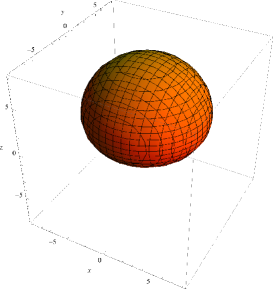
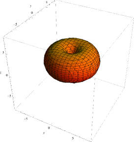
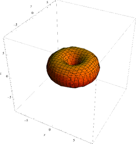
Figure 1: Density contours of the squared zero-mode (3.49) for $j=4$ and $p=12$ and, from left to right, $m=-4,m=-2,m=0$

4 Conclusion

We end with some general observations and comments on our results. Having understood the $SU(2)$ transformation properties of the zero-modes, it remains a puzzle why $SU(2)$ representations with a range of different spins are degenerate in the kernel of $\not{D}_{p}$. The degeneracy grows quadratically in the ‘quantum number’ $[|p|]$ and is reminiscent of generic energy eigenspaces for the Hamiltonian of the non-relativistic hydrogen atom and, closer to the current context, for the Laplace and the Dirac operator on the Taub-NUT space (not twisted by a connection). In all cases, the degeneracy can be understood in terms of an additional conserved vector operator - the quantum analogue of the Runge-Lenz vector [28]. We have not investigated generalisations of this operator for the twisted Dirac operators studied here. In any case, an argument based on symmetry would not be entirely satisfactory since the index of the operator is invariant under small changes of both the metric and the connection which would destroy any symmetry. For a topological degeneracy like the one studied here, one expects there to be a more robust reason.

Our discussion could be extended and generalised to the multicentre Taub-NUT space, for which the dimension of the kernel of an appropriate Dirac operator was already given by Pope in [7] as the dimension (1.2) times the number of centres. Other interesting four-manifolds with natural candidates for line bundles and connections are the Atiyah-Hitchin manifold, the complex projective plane with the Fubini-Study metric as well the Hitchin family of 4-manifolds which interpolates between them. All of these spaces are described in [8], where they are proposed as possible geometric models for elementary particles.

In the interpretation of the Taub-NUT manifold as a geometric model for the electron in [8], zero-modes of the Dirac operator were proposed as possible carriers of the spin 1/2 degrees of freedom of the electron. With the length scale $L$ of the Taub-NUT manifold identified with the classical electron radius as proposed in [8], the zero-modes are localised to the size of the classical electron radius. Focusing on positive $p$, our discussion also shows that the kernel of $\not{D}_{p}$ does indeed contain a normalisable doublet of spin 1/2 states, provided we pick $p>2$. To obtain spin at most 1/2, we need $p\leq 3$, but even with this choice we retain a spin 0 singlet as well. We have not been able to eliminate the spin 0 state by any natural condition.

However, we note that spin 1/2 states have one special property among all the zero-modes. By picking $p=2$, the spin 1/2 doublet has the functional dependence

$$\sqrt{\frac{r}{r+L}}(a_{-1}z_{1}+a_{1}z_{2}),$$ (4.1)

which tends to $SU(2)$ doublet states in their standard form $a_{-1}z_{1}+a_{1}z_{2}$ as $r\rightarrow\infty$. Uniquely among the zero-modes, spin 1/2 states can be made to neither decay to zero nor blow up at spatial infinity by a choice of $p$. With the same choice $p=2$, the square (3.49) of the spin 0 state is exponentially localised at the origin, with characteristic size $L$. It is proportional to

$$\frac{e^{-\frac{r}{L}}}{r+L}.$$ (4.2)

Borrowing supersymmetry jargon, the choice $p=2$ therefore gives a totally delocalised spin 1/2 ‘soul’ and an exponentially localised spin 0 ‘body’.

Acknowledgements   RJ thanks the School of Mathematical and Computer Sciences at Heriot-Watt University for a Global Platform PhD Scholarship. BJS thanks Michael Singer for discussions about Dirac operators coupled to monopoles.

Appendix A Background and conventions

A.1 Parametrising $SU(2)$

Our conventions and coordinates in this paper are designed to be convenient for describing the Hopf map, harmonic analysis on $S^{3}$ and sections of powers of the hyperplane bundle over $S^{2}$. To achieve this, we picked different conventions from those in [29, 30, 31, 8] which study closely related material. In particular, our $\mathfrak{su}(2)$ generators have the opposite sign of the ones used in those papers. As a result, the left-invariant forms and vector fields change sign. Our choice of Euler angles is also different.

To parametrise the group $SU(2)$, we use the $\mathfrak{su}(2)$ generators

$$t_{j}=-\frac{i}{2}\tau_{j},\;j=1,2,3,$$ (A.1)

where $\tau_{a}$ are the Pauli matrices; the commutators are $[t_{i},t_{j}]=\epsilon_{ijk}t_{k}$. We then pararmetrise $h\in SU(2)$ in terms of Euler angles $\beta\in[0,\pi)$, $\alpha\in[0,2\pi)$ and $\gamma\in[0,4\pi)$ as follows

$$h=e^{\alpha t_{3}}e^{\beta t_{2}}e^{\gamma t_{3}}=\begin{pmatrix}e^{-\frac{i}{2}(\gamma+\alpha)}\cos\frac{\beta}{2}&-e^{\frac{i}{2}(\gamma-\alpha)}\sin\frac{\beta}{2}\\ e^{\frac{i}{2}(\alpha-\gamma)}\sin\frac{\beta}{2}&e^{\frac{i}{2}(\gamma+\alpha)}\cos\frac{\beta}{2}\end{pmatrix}.$$ (A.2)

We also use an alternative parametrisation in terms of a complex unit vector $(z_{1},z_{2})$ as

$$h=\begin{pmatrix}z_{1}&-\bar{z}_{2}\\ z_{2}&\phantom{-}\bar{z}_{1}\end{pmatrix},$$ (A.3)

with the constraint $|z_{1}|^{2}+|z_{2}|^{2}=1$ understood. Comparing with (A.2), we have

$$z_{1}=e^{-\frac{i}{2}(\alpha+\gamma)}\cos\frac{\beta}{2},\quad z_{2}=e^{\frac{i}{2}(\alpha-\gamma)}\sin\frac{\beta}{2}.$$ (A.4)

A.2 Forms and vector fields on $SU(2)$

With $h\in SU(2)$ and the generators $t_{j},\;j=1,2,3$, defined in (A.1) we define the left-invariant 1-forms on $SU(2)$ via

$$h^{-1}dh=\sigma_{1}t_{1}+\sigma_{2}t_{2}+\sigma_{3}t_{3}\,.$$ (A.5)

For the Euler angle parametrisation (A.2) we compute to find

$$\sigma_{1} =\sin\gamma d\beta-\cos\gamma\sin\beta d\alpha,$$

$$\sigma_{2} =\cos\gamma d\beta+\sin\gamma\sin\beta d\alpha,$$

$$\sigma_{3} =d\gamma+\cos\beta d\alpha.$$ (A.6)

These forms satisfy $d\sigma_{i}=-\frac{1}{2}\epsilon_{ijk}\sigma_{j}\wedge\sigma_{k}$.

The dual vector fields $X_{j}$, $j=1,2,3$, are left-invariant and generate the infinitesimal right-action

$$X_{j}:h\mapsto ht_{j},\quad j=1,2,3.$$ (A.7)

Their commutators are

$$[X_{i},X_{j}]=\epsilon_{ijk}X_{k}.$$ (A.8)

In the main text we often use the combinations

$$X_{+}=X_{1}+iX_{2},\qquad X_{-}=X_{1}-iX_{2},$$ (A.9)

which satisfy

$$[iX_{3},X_{\pm}]=\pm X_{\pm},$$ (A.10)

and therefore act as raising (+) and lowering (-) operators for $iX_{3}$. In terms of Euler angles we find

$$X_{1} =\phantom{-}\cot\beta\cos\gamma\partial_{\gamma}+\sin\gamma\partial_{\beta}-\frac{\cos\gamma}{\sin\beta}\partial_{\alpha},$$

$$X_{2} =-\cot\beta\sin\gamma\partial_{\gamma}+\cos\gamma\partial_{\beta}+\frac{\sin\gamma}{\sin\beta}\partial_{\alpha},$$

$$X_{3} =\phantom{-}\partial_{\gamma},$$ (A.11)

so that

$$X_{+}=ie^{-i\gamma}\left(\partial_{\beta}+i\frac{1}{\sin\beta}\partial_{\alpha}\ -i\frac{\cos\beta}{\sin\beta}\partial_{\gamma}\right),\quad X_{-}=-ie^{i\gamma}\left(\partial_{\beta}-i\frac{1}{\sin\beta}\partial_{\alpha}+i\frac{\cos\beta}{\sin\beta}\partial_{\gamma}\right).$$ (A.12)

We also require the left-invariant 1-forms and vector fields in complex notation. With (A.3), we find

$$\sigma_{1}+i\sigma_{2}=2i(z_{1}dz_{2}-z_{2}dz_{1}),\qquad\sigma_{3}=2i(\bar{z}_{1}dz_{1}+\bar{z}_{2}dz_{2}).$$ (A.13)

To compute the dual vector fields in complex notation we use

$$t_{+}=t_{1}+it_{2}=-i\begin{pmatrix}0&1\\ 0&0\end{pmatrix},\quad t_{-}=t_{1}-it_{2}=-i\begin{pmatrix}0&0\\ 1&0\end{pmatrix}.$$ (A.14)

Then, from the rule (A.7) we have, for example.

$$X_{+}:\begin{pmatrix}z_{1}&-\bar{z}_{2}\\ z_{2}&\bar{z}_{1}\end{pmatrix}\mapsto-i\begin{pmatrix}z_{1}&-\bar{z}_{2}\\ z_{2}&\bar{z}_{1}\end{pmatrix}\begin{pmatrix}0&1\\ 0&0\end{pmatrix}.$$ (A.15)

Evaluating, we find

$$X_{+} =i(z_{1}\bar{\partial}_{2}-z_{2}\bar{\partial}_{1}),$$

$$X_{-} =i(\bar{z}_{2}\partial_{1}-\bar{z}_{1}\partial_{2}),$$

$$X_{3} =\frac{i}{2}(\bar{z}_{1}\bar{\partial}_{1}+\bar{z}_{2}\bar{\partial}_{2}-z_{1}\partial_{1}-z_{2}\partial_{2}).$$ (A.16)

One checks that

$$\sigma_{+}(X_{-})=\sigma_{-}(X_{+})=2,\quad\sigma_{3}(X_{3})=1,$$ (A.17)

with all other pairings vanishing.

Similarly, for left-generated and right-invariant vector fields

$$Z_{i}:h\mapsto-t_{i}h,$$ (A.18)

we define $Z_{\pm}=Z_{1}\pm iZ_{2}$ and find

$$Z_{+} =i(z_{2}\partial_{1}-\bar{z}_{1}\bar{\partial}_{2}),$$

$$Z_{-} =i(z_{1}\partial_{2}-\bar{z}_{2}\bar{\partial}_{1}),$$

$$Z_{3} =\frac{i}{2}(z_{1}\partial_{1}-z_{2}\partial_{2}-\bar{z}_{1}\bar{\partial}_{1}+\bar{z}_{2}\bar{\partial}_{2}).$$ (A.19)

They satisfy $[Z_{i},Z_{j}]=\epsilon_{ijk}Z_{k}$ (and hence $[iZ_{3},Z_{\pm}]=\pm Z_{\pm}$) and commute with the right-generated vector fields $X_{j}$, $j=1,2,3$.

A.3 Harmonic analysis on $S^{3}$ in complex coordinates

The Laplace operator on $SU(2)$ acting on functions on $SU(2)$ can be written as

$$\Delta_{S^{3}}=X_{1}^{2}+X_{2}^{2}+X_{3}^{2}=Z_{1}^{2}+Z_{2}^{2}+Z_{3}^{2}.$$ (A.20)

It commutes with left- and right-generated vector fields, and its eigenspaces can therefore be decomposed into irreducible representations of $\mathfrak{su}(2)\oplus\mathfrak{su}(2)$, generated by $X_{j}$ and $Z_{j}$, $j=1,2,3$. Here, we are only interested in the decomposition of functions on $SU(2)$ into irreducible representations under the $SU(2)$ left-action, generated by $Z_{j}$, $j=1,2,3$. Since these generators commute with $iX_{3}$ and $\Delta_{S^{3}}$, we can fix the eigenvalues of both $iX_{3}$ and $\Delta_{S^{3}}$. We now show how to obtain the irreducible representations under the $SU(2)$ actions in this way, using complex coordinates.

We use the trick of abandoning the constraint $|z_{1}|^{2}+|z_{2}|^{2}$ and considering functions defined on all of $\mathbb{C}^{2}$, see [12] for an analogous treatment of the Laplace operator on $S^{2}$. In order to obtain irreducible representations of $SU(2)$ we need to impose the constraint that the Laplace operator on $\mathbb{C}^{2}\simeq\mathbb{R}^{4}$

$$\Box_{4}=4(\partial_{1}\bar{\partial}_{1}+\partial_{2}\bar{\partial_{2}})$$ (A.21)

vanishes.

To see how and why this works, we define differential operators on $\mathbb{C}^{2}$

$$D=\frac{1}{2}(z_{1}\partial_{1}+z_{2}\partial_{2}),\qquad\bar{D}=\frac{1}{2}(\bar{z}_{1}\bar{\partial}_{1}+\bar{z}_{2}\bar{\partial}_{2}),$$ (A.22)

and observe that both $D$ and $\bar{D}$ commute with $Z_{\pm},Z_{3}$ and that

$$iX_{3}=D-\bar{D}.$$ (A.23)

We also find that

$$X_{+}X_{-}=-4D\bar{D}-2D+(|z_{1}|^{2}+|z_{2}|^{2})(\partial_{1}\bar{\partial}_{1}+\partial_{2}\bar{\partial_{2}}),$$ (A.24)

and therefore have the identity

$$\Delta_{S^{3}} =X_{+}X_{-}+(D-\bar{D})-(D-\bar{D})^{2}$$

$$=-(D+\bar{D})^{2}-(D+\bar{D})+(|z_{1}|^{2}+|z_{2}|^{2})(\partial_{1}\bar{\partial}_{1}+\partial_{2}\bar{\partial_{2}}).$$ (A.25)

Defining

$$J=D+\bar{D},$$ (A.26)

we conclude that

$$\Delta_{S^{3}}F=-J(J+1)F,\qquad\text{provided}\quad\Box_{4}F=0.$$ (A.27)

Picking half integers $N,\bar{N}\in\frac{1}{2}\mathbb{N}_{0}$ and $m,\bar{m}\in\frac{1}{2}\mathbb{Z}$ in the range

$$m\in\{-N,-N+1,\ldots,N-1,N\},\quad\bar{m}\in\{-\bar{N},\bar{N}+1,\ldots,\bar{N}-1,\bar{N}\},$$ (A.28)

and defining a monomial

$$F_{Nm\bar{N}\bar{m}}=z_{1}^{N-m}z_{2}^{N+m}\bar{z}_{1}^{\bar{N}+\bar{m}}\bar{z}_{2}^{\bar{N}-\bar{m}},$$ (A.29)

one checks that

$$DF_{Nm\bar{N}\bar{m}}=NF_{Nm\bar{N}\bar{m}},\quad\bar{D}F_{Nm\bar{N}\bar{m}}=\bar{N}F_{Nm\bar{N}\bar{m}},\$$ (A.30)

and hence

$$JF_{Nm\bar{N}\bar{m}}=(N+\bar{N})F_{Nm\bar{N}\bar{m}},\qquad iX_{3}F_{Nm\bar{N}\bar{m}}=(N-\bar{N})F_{Nm\bar{N}\bar{m}}.$$ (A.31)

We can now see that imposing the annihilation by $\Box_{4}$ projects out an irreducible representation of $SU(2)$ as follows. We fix the eigenvalues $N$ and $\bar{N}$, and hence also $j:=N+\bar{N}$ and $s:=N-\bar{N}$. Then we write $P_{(N,\bar{N})}$ for the space of polynomials in $z_{1},z_{2},\bar{z}_{1},\bar{z}_{2}$ with fixed values $N,\bar{N}$. Thus, $P_{(N,\bar{N})}$ has dimension $(2N+1)(2\bar{N}+1)$. It is easy to check that

$$\Box:P_{(N,\bar{N})}\rightarrow P_{(N-\frac{1}{2},\bar{N}-\frac{1}{2})}$$ (A.32)

is surjective. As a result, the kernel has dimension

$$d=(2N+1)(2\bar{N}+1)-4N\bar{N}=2(N+\bar{N})+1=2j+1.$$ (A.33)

The monomial $F_{NN\bar{N}\bar{N}}$ is in this space , and is an eigenstate of $iZ_{3}$:

$$iZ_{3}F_{NN\bar{N}\bar{N}}=(N+\bar{N})F_{NN\bar{N}\bar{N}}=jF_{NN\bar{N}\bar{N}}.$$ (A.34)

Acting with the lowering operator $Z_{-}$ we generate the $(2j+1)$-dimensional irreducible representation of $SU(2)$, as claimed.

We are not going to give a basis for this space in the general case, but note two special cases which are used in the main text. When $s=j$, we have $\bar{N}=0,N=j$ and obtain the (non-normalised) holomorphic basis

$$z_{1}^{j-m}z_{2}^{j+m},\qquad m=-j,-j+1,\ldots,j-1,j,$$ (A.35)

with elements labelled by the eigenvalue $m$ of $iZ_{3}$. When $s=-j$, we have $N=0,\bar{N}=j$ and obtain the (non-normalised) antiholomorphic basis

$$\bar{z}_{1}^{j+m}\bar{z}_{2}^{j-m},\qquad m=-j,-j+1,\ldots,j-1,j,$$ (A.36)

with elements again labelled by the eigenvalue $m$ of $iZ_{3}$.

A.4 Lens spaces and the Hopf fibration

Identifying $S^{3}$ with $SU(2)$, the Hopf map $S^{3}\rightarrow S^{2}$ is defined by taking the quotient of $SU(2)$ by a $U(1)$ right action. To make this concrete we pick the torus generated by $t_{3}$ to define the right action

$$R(e^{i\delta}):h\mapsto he^{\delta t_{3}},\quad\delta\in[0,4\pi).$$ (A.37)

In terms of Euler angles, this is simply the shift $\gamma\mapsto\gamma+\delta$. In terms of the complex coordinates $(z_{1},z_{2})$, the map reads

$$R(e^{i\delta}):(z_{1},z_{2})\mapsto(z_{1}e^{-i\frac{\delta}{2}},z_{2}e^{-i\frac{\delta}{2}}).$$ (A.38)

The infinitesimal generator is the vector field $X_{3}$ in (1.6).

We need to generalise our discussion to include the Lens space $L(1,n)=S^{3}/\mathbb{Z}_{n}$, obtained from $S^{3}$ by the right action of the cyclic group $\mathbb{Z}_{n}$, $n\neq 0$, whose generator acts via

$$h\mapsto he^{\frac{4\pi}{n}t_{3}},\qquad(z_{1},z_{2})\mapsto(z_{1}e^{-i\frac{2\pi}{n}},z_{2}e^{-i\frac{2\pi}{n}}).$$ (A.39)

The $U(1)$ right-action is as in (A.37) but with $\delta\in[0,4\pi/n)$. As a result the associated basis of the $U(1)$ Lie algebra is $ni/2$. The vector field on $SU(2)$ generated by the $U(1)$ right-action is still $X_{3}$, but is now the push-forward of the $U(1)$ generator $ni/2$:

$$R_{*}\left(n\frac{i}{2}\right)=X_{3}.$$ (A.40)

The Hopf map can be written concretely as a projection from $L(1,n)$ onto the unit 2-sphere inside the Lie algebra $\mathfrak{su}(2)$. The following formula holds strictly only for $S^{3}$, but it makes sense for $L(1,n)$, too, since the image is manifestly invariant under (A.39):

$$\pi:S^{3}\rightarrow S^{2}\subset\mathfrak{su}(2),\quad h\mapsto ht_{3}h^{-1}.$$ (A.41)

In terms of the Euler angle parametrisation (A.2),

$$\pi(h)=(\sin\beta\cos\alpha)t_{1}+(\sin\beta\sin\alpha)t_{2}+(\cos\beta)t_{3},$$ (A.42)

so that our choice of Euler angles induces $(\beta,\alpha)$ as standard spherical polar coordinates on the 2-sphere.

We introduce complex coordinates on $S^{2}$ by stereographic projection. Writing $N$ for the ‘North Pole’ $(0,0,1)\in S^{2}$ and $S$ for the ‘South Pole’ $(0,0,-1)\in S^{2}$, we define

$$U_{N}=S^{2}\setminus\{S\},\qquad U_{S}=S^{2}\setminus\{N\}.$$ (A.43)

Then, in terms the coordinates (A.42), stereographic projection from the South Pole is

$$\text{St}:U_{N}\subset S^{2}\rightarrow\mathbb{C},\qquad(n_{1},n_{2},n_{3})\mapsto z=\frac{n_{1}+in_{2}}{1+n_{3}},$$ (A.44)

and stereographic projection from the North Pole, followed by complex conjugation is

$$\bar{\text{St}}:U_{S}\subset S^{2}\rightarrow\mathbb{C},\qquad(n_{1},n_{2},n_{3})\mapsto\zeta=\frac{n_{1}-in_{2}}{1-n_{3}}.$$ (A.45)

Thus $\zeta=1/z$ and we observe that

$$z=\frac{z_{2}}{z_{1}}=\tan\frac{\beta}{2}e^{i\alpha},\qquad\zeta=\frac{z_{1}}{z_{2}}=\cot\frac{\beta}{2}e^{-i\alpha}.$$ (A.46)

In other words, in complex coordinates, the Hopf map followed stereographic project from the South Pole is

$$\text{St}\circ\pi:S^{3}\rightarrow U_{N},\quad(z_{1},z_{2})\mapsto z,$$ (A.47)

while the Hopf map followed by stereographic projection from the North Pole and complex conjugation is

$$\bar{\text{St}}\circ\pi:S^{3}\rightarrow U_{S},\quad(z_{1},z_{2})\mapsto\zeta.$$ (A.48)

In our discussion we also require local sections of the Hopf bundle in both complex coordinates and Euler angles. We use the same notation for both and write, on the northern patch,

$$s_{N}:U_{N}\rightarrow S^{3},\quad z\mapsto\frac{1}{\sqrt{1+|z|^{2}}}(1,z),\qquad(\beta,\alpha)\mapsto e^{\alpha t_{3}}e^{\beta t_{2}}e^{-\alpha t_{3}}$$ (A.49)

and on the southern patch

$$s_{S}:U_{S}\rightarrow S^{3},\quad\zeta\mapsto\frac{1}{\sqrt{1+|\zeta|^{2}}}(\zeta,1),\qquad(\beta,\alpha)\mapsto e^{\alpha t_{3}}e^{\beta t_{2}}e^{\alpha t_{3}}.$$ (A.50)

A.5 Associated line bundles and their sections

Our discussion in the main text frequently describes sections of line bundles associated to the Lens spaces in terms of equivariant functions

$$F:L(1,n)\rightarrow\mathbb{C},$$ (A.51)

i.e., functions which satisfy

$$F(he^{\delta t_{3}})=e^{-i\frac{n}{2}\delta}F(h),\quad\delta\in\left[0,\frac{4\pi}{n}\right],$$ (A.52)

or, in complex coordinates,

$$F(\lambda z_{1},\lambda z_{2})=\lambda^{n}F(z_{1},z_{2}),$$ (A.53)

where we wrote $\lambda=e^{-i\delta/2}$. In order to minimise notation, we use $h$ also for elements of $L(1,n)$ here (rather than equivalence classes). Infinitesimally, the equivariance condition can be expressed as

$$iX_{3}F=\frac{n}{2}F.$$ (A.54)

We can obtain local sections on the patches $U_{N}$ and $U_{S}$ via pull-back with (A.49) and (A.50):

$$f_{N}=s_{N}^{*}F,\qquad f_{S}=s_{S}^{*}F.$$ (A.55)

Using (A.53) and

$$f_{N}(z)=F\left(\frac{1}{\sqrt{q}}(1,z)\right),\quad f_{S}(z)=F\left(\sqrt{\frac{\bar{z}}{z}}\frac{1}{\sqrt{q}}(1,z)\right),$$ (A.56)

one deduces the patching condition

$$f_{S}=e^{-in\alpha}f_{N}=\left(\frac{\bar{z}}{z}\right)^{\frac{n}{2}}f_{N}.$$ (A.57)

The line bundle associated to $L(1,n)$ is often denoted as $H^{n}$, the $n$th tensor power of the hyperplane bundle $H$. The latter is the dual bundle of the tautological line bundle $L$ over $\mathbb{CP}^{1}$ whose fibre over a point $\ell\in\mathbb{CP}^{1}$ is the line in $\mathbb{C}^{2}$ defined by $\ell$:

$$L=\{(l,(w_{1},w_{2})\subset\mathbb{CP}_{1}\times\mathbb{C}^{2}|(w_{1},w_{2})\in l\}.$$ (A.58)

For the hyperplane bundle $H$ over $\mathbb{CP}^{1}$, the fibre over a point $\ell\in\mathbb{CP}^{1}$ is the dual space $\ell^{*}$. In the equivariant language (A.53), holomorphic sections of $H^{n}$, $n\geq 0$, can be written as homogeneous polynomials of degree $n$ in the variables $z_{1},z_{2}$:

$$F(z_{1},z_{2})=\sum_{k=0}^{n}a_{k}z_{1}^{n-k}z_{2}^{k}.$$ (A.59)

The space of all holomorphic sections can then be identified with the $(n+1)$-dimensional space of all such polynomials. As we shall check below, the Chern number of $H^{n}$ is $n$.

A.6 Invariant connections and the Dirac monopole

The magnetic monopole of charge $n\neq 0$ is the curvature of the rotationally invariant $U(1)$ connection on the Lens space $L(1,n)$. Using (A.40), the requirement for a 1-form $\mathcal{A}$ to be a connection 1-form on $L(1,n)$ is

$$\mathcal{A}(X_{3})=\frac{in}{2},$$ (A.60)

while ‘rotationally invariant’ means invariant under the left-action of $SU(2)$ on $L(1,n)$. The form

$$\mathcal{A}=\frac{in}{2}\sigma_{3}=\frac{in}{2}\left(d\gamma+\cos\beta\,d\alpha\right).$$ (A.61)

satisfies both these requirements. Its curvature is

$$F=d\mathcal{A}=-\frac{in}{2}\sin\theta d\beta\wedge d\alpha,$$ (A.62)

which is the field of the Dirac magnetic monopole.

We obtain the local gauge potentials via pull-back with the local sections (A.49) and (A.50):

$$s^{*}_{N}\mathcal{A}=A^{n}_{N}=\frac{in}{2}(-1+\cos\beta)d\alpha,\quad s^{*}_{S}\mathcal{A}=A^{n}_{S}=\frac{in}{2}(1+\cos\theta)d\alpha.$$ (A.63)

The potentials are related by the $U(1)$ gauge transformation

$$A_{S}^{n}=A_{N}^{n}+g_{SN}dg_{SN}^{-1},\qquad g_{SN}(\alpha)=e^{-in\alpha},$$ (A.64)

and satisfy $F=dA_{N}^{n}=dA_{S}^{n}$. The charge $n$ must be an integer by the Dirac quantisation condition and equals the Chern number of the bundle

$$\frac{i}{2\pi}\int_{S^{2}}F=n.$$ (A.65)

Since the potential $A^{n}_{N}$ is well defined on $U_{N}$ we rewrite it in terms of $z$ and $q$ as

$$A_{N}^{n}=\frac{n}{2q}(zd\bar{z}-\bar{z}dz),$$ (A.66)

Similarly, on $U_{S}$, we have

$$A_{S}^{n}=\frac{n}{2}\frac{\zeta d\bar{\zeta}-\bar{\zeta}d\zeta}{1+|\zeta|^{2}}.$$ (A.67)

For the curvature we find

$$F=n(dz_{1}\wedge d\bar{z}_{1}+dz_{2}\wedge d\bar{z}_{2})=n\frac{dz\wedge d\bar{z}}{(1+|z|^{2})^{2}}=n\frac{d\zeta\wedge d\bar{\zeta}}{(1+|\zeta|^{2})^{2}},$$ (A.68)

with the equalities holding wherever the expressions are defined.

A.7 Conventions related to the Dirac operator

We will use the following conventions when writing down the Dirac operator on a Riemannian manifold. Introducing and $n$-bein of 1-forms $e_{1},\ldots,e_{n}$ so that the metric is

$$ds^{2}=e_{1}^{2}+\ldots+e_{n}^{2},$$ (A.69)

we solve

$$de_{a}+\omega_{ab}\wedge e_{b}=0,$$ (A.70)

for the spin connection 1-forms $\omega_{ab}=-\omega_{ba}$, $a,b=1,\ldots,n$. In terms of the dual vector fields $E_{a}$ defined via

$$e_{a}(E_{b})=\delta_{ab},$$ (A.71)

and $\gamma$-matrices satisfying

$$\{\gamma_{a},\gamma_{b}\}=-2\delta_{ab},$$ (A.72)

the spin connection is

$$\Gamma=-\frac{1}{8}[\gamma_{a},\gamma_{b}]\omega^{ab}.$$ (A.73)

The Dirac operator takes the form

$$\not{D}=\gamma^{c}\iota_{E_{c}}(d+\Gamma)=\gamma^{c}\left(E_{c}-\frac{1}{8}[\gamma_{a},\gamma_{b}]\omega^{ab}_{c}\right),$$ (A.74)

where $\omega^{ab}_{c}=\omega^{ab}(E_{c})$, and indices are moved up or down for convenience. When we twist the bundle of spinors with an additional $U(1)$ bundle with connection $A$, the twisted Dirac operator is

$$\not{D}_{A}=\gamma^{c}\iota_{E_{c}}(d+A+\Gamma)=\gamma^{c}\left(E_{c}+A_{c}-\frac{1}{8}[\gamma_{a},\gamma_{b}]\omega^{ab}_{c}\right).$$ (A.75)

References

• [1] M. F. Atiyah and I. M. Singer, The index of elliptic operators: I, Ann. of Math. 87 (1968) 484–530.
• [2] Joseph C. Várilly, An introduction to noncommutative Geometry, EMS Series of Lectures in Mathematics, European Mathematical Society Publishing House, 2006.
• [3] L. Erdös and J. P. Solovej, The kernel of the Dirac operator on $S^{3}$ and $\mathbb{R}^{3}$, Rev. Math. Phys. 13 (2001) 1247–1280.
• [4] R. D. Sorkin, Kaluza-Klein monopole, Phys. Rev. Lett. 51 (1983) 87.
• [5] D. J. Gross and M. J. Perry, Magnetic monopoles in Kaluza-Klein theories, Nucl. Phys. B226 (1983) 29–48.
• [6] C. N. Pope, Axial-vector anomalies and the index theorem in charged Schwarzschild and Taub-NUT spaces, Nucl. Phys. B141 (1978) 432–444.
• [7] C. N. Pope, The $\eta$-invariant of charged spinors in Taub-NUT, J. Phys. A: Math. Gen. 14 (1981) L133-L137.
• [8] M. Atiyah, N. S. Manton and B. J. Schroers, Geometric models of matter, Proc. Roy. Soc. Lond. A468 (2012) 1252–1279.
• [9] T. Dray, The Relationship between monopole harmonics and spin weighted spherical harmonics, J. Math. Phys. 26 (1985) 1030.
• [10] T. Dray, A unified treatment of Wigner $\mathcal{D}$ functions, spin-weighted spherical harmonics, and monopole harmonics, J. Math. Phys. 27 (1986) 781–792.
• [11] M. Göckeler and T. Schücker, Differential geometry, gauge theories, and gravity, Cambridge University Press, Cambridge, 1987.
• [12] S. Sternberg, Group theory and physics, Cambridge University Press, Cambridge 1994.
• [13] E. T. Newman and R. Penrose, Note on the Bondi-Metzner-Sachs group, J. Math. Phys. 7 (1966) 863–870.
• [14] J. N. Goldberg, A. J. MacFarlane, E. T. Newman, F. Rohrlich and E. C. G. Sudarshan, Spin-$s$ spherical harmonics and $\eth$, J. Math. Phys. 8 (1967) 2155–2161.
• [15] R. Jackiw and C. Rebbi, Solitons with fermion number 1/2, Phys. Rev. D 13 (1976) 3398–3409.
• [16] C. Callias, Axial anomalies and index theorems on open spaces, Commun. Math. Phys. 62 (1978) 213–234.
• [17] C. Callias, Spectra of fermions in monopole fields - exactly soluble models, Phys. Rev. D 16 (1977) 3068–3077.
• [18] W. Nahm, On abelian selfdual multi-monopoles, Phys. Lett. B93 (1980) 42–46.
• [19] B. Cheng and C. Ford, Fermion zero modes for abelian BPS monopoles, Phys. Lett. B720 (2013) 262–264.
• [20] T. Eguchi, P. B. Gilkey and A. J. Hanson, Gravitation, gauge theories and differential geometry, Phys. Rep. 66 (1980) 213–393.
• [21] A. Comtet and P. A. Horvathy, The Dirac equation in Taub-NUT space, Phys. Lett. B349 (1995) 49–56.
• [22] S. Sethi, M. Stern and E. Zaslow, Monopole and Dyon bound states in N=2 supersymmetric Yang-Mills theories, Nucl. Phys. B457 (1995) 484–512.
• [23] K. Lee, E. J. Weinberg and P. Yi, Electromagnetic duality and $SU(3)$ monopoles, Phys. Lett. B376 (1996) 97–102.
• [24] J. P. Gauntlett and D. A. Lowe, Dyons and S-duality in $N=4$ supersymmetric gauge theory, Nucl. Phys. B472 (1996) 194–20.
• [25] Z. F. Ewaza and A. Iwazaki, Monopole-fermion dynamics and the Rubakov effect in Kaluza-Klein theories, Phys. Lett. B138 (1984) 81–86.
• [26] M. Kobayahsi and A. Sugamoto, Fermions in the background field of the Kaluza-Klein monopole, Progr. Theor. Phys. 72 (1984) 122–133.
• [27] A. Bais and P. Batenburg, Fermion dynamics in the Kaluza-Klein monopole geometry, Nucl. Phys. B245(1984) 469–480.
• [28] M Visinescu, Generalized Runge-Lenz vector in Taub-NUT spinning space, Phys. Lett. B339 (1994) 28–34.
• [29] G. W.  Gibbons and N. S.  Manton, Classical and quantum dynamics of BPS monopoles, Nucl. Phys. B274 (1986) 183–224.
• [30] N. S. Manton and B. J. Schroers, Bundles over moduli spaces and the quantization of BPS monopoles, Annals Phys. 225 (1993) 290–338.
• [31] B. J. Schroers, Quantum scattering of BPS monopoles at low energy, Nucl. Phys. B367 (1991) 177–214.