TURBULENCE-LEVEL VARIATIONS AND MAGNETIC FIELD ORIENTATIONS IN THE FAST SOLAR WIND

Abstract

The turbulent magnetic fields of a large set of fast solar wind streams measured onboard ACE and STEREO A and B are analyzed in an effort to identify the effects of the turbulence-level broad variations on the orientations of the local, time-averaged magnetic fields. The power level of turbulence, roughly defined as the power in the transverse field fluctuations normalized to the medium-scale average background field, tightly orders the location of the peaks in the probability distribution functions (PDFs) of the angles between local fields and Parker spiral. As a result, the broad variations in the power level of turbulence cause a steep dependence of the average power level of turbulence on the angle of the local field to the Parker spiral, with the highest turbulence levels found near the normal to the Parker spiral and the lowest levels near the Parker spiral direction. Generalized quasilinear estimates of the mean cross-field displacements adapted to intermittent time-varying turbulence lead to accurate fits of the observed angle PDFs at all stable levels of turbulence, supporting the idea that isotropic turbulence could account for the observed angle PDFs. Modeling of the angles $\alpha_{r}$ between local fields and radial direction, from the PDFs of the angles $\alpha$ between local and background fields under an assumption of axisymmetry of the turbulent fields around a background field in or near the direction of the Parker spiral, also produces fairly good fits of the observed PDFs of $\alpha_{r}$, thereby validating the assumption. Finally, local field reversals are found to be quite common even within very broad streams of “unipolar” fast solar wind.

1. INTRODUCTION

Local spectral analysis of the solar wind (SW) magnetic fields reveals strong time variations in the power level of the turbulent field fluctuations. This variability of the power level of the field fluctuations is responsible for the strong non-Gaussianity of the observed PDFs of field variations associated with intermittency (Ragot 2013). The strong non-Gaussianity of the observed PDFs of field variations is unlikely to be the only observable consequence of the power-level variability. Here, we investigate the magnetic field orientations as functions of the highly varying power level of turbulence in the fast SW, and vice versa, where the power level of turbulence is defined with the field fluctuations normalized to the medium-scale ($15\,$min) average background field.

SW magnetic fields ${\bf B}$ are measured along SW flow lines and the time series of these in situ field measurements can be averaged on a timescale $\Delta t$ to obtain mean “magnetic field vectors” ${\bf B}_{\mbox{{\small av}}}(t,\Delta t)$. If $\delta t$ is the time resolution of the measurements and $\Delta t=N\delta t$,

$${\bf B}_{\mbox{{\small av}}}(t,\Delta t)={1\over N+1}\sum_{n=-N/2}^{N/2}{\bf B}(t+n\delta t)\;.$$ (1)

What is the meaning of these mean “magnetic field vectors” ${\bf B}_{\mbox{{\small av}}}(t,\Delta t)$? Do they somehow give the direction of a real magnetic field within the SW? How do they relate to the direction of “real” magnetic field lines? The answer depends on how much magnetic field lines diverge from each other, locally, and on how much transport they undergo collectively. If the directions of neighboring field lines strongly deviate from each other rather than being dominated by one common direction of transport, then it is dubious that the mean “magnetic field vectors” ${\bf B}_{\mbox{{\small av}}}$ can be ascribed any other meaning than that of time averages of in situ magnetic fields along SW flow lines. However, if the directions of neighboring field lines mostly run “parallel” to each other, being dominated by one common direction of transport, then the mean “magnetic field vectors” ${\bf B}_{\mbox{{\small av}}}$ give the mean local common direction of transport, or mean local direction of a field line that passes through one of the measurement points.

In a magnetic turbulence with background field ${\bf B}_{0}$, such as the SW, both the field-line dispersal (relative field-line divergence) and global field-line transport (common transport) can be assessed theoretically and modeled (e.g., Ragot 1999, 2006a, 2006b, 2009, 2010a, 2010b, 2011). Field-line dispersal and global field-line transport are measured by the variations in field-line separations and by the field-line displacements across the background-field direction, or cross-field displacements, $\Delta r$, respectively. It appears that in slow and fast SW streams, the association between time-averaged field vector direction and mean direction of an actual field line is justified on most timescales because the cross-field displacements $\Delta r$ far exceed the variations in field-line separations on the background field-aligned length scales $\Delta z\leq 10^{11}$cm (e.g., Ragot 2010b, knowing that $\langle(\Delta r)^{2}\rangle^{1/2}\sim\Delta z$ on these $\Delta z$ scales).^, For a SW speed $V_{\mbox{{\small sw}}}$, the length scales $\Delta z$ relate to the timescales $\Delta t$ through $\Delta z=V_{\mbox{{\small sw}}}\,\Delta t\,\cos\phi_{r}$, the angle $\phi_{r}$ between Parker spiral and radial direction being defined below in Equation (2).

The time-averaged field directions obtained by integrating in situ fast SW magnetic fields over time intervals of duration $\Delta t\sim 15-20\,$s (depending on $V_{\mbox{{\small sw}}}$) should therefore match the local field-line directions on the background field-aligned length scale $\Delta z\sim 10^{9}\,$cm. And the angles $\alpha$ [see Equation (14) in Section 4] between these time-averaged in situ fields and the background field ${\bf B}_{0}$ should match the angles between the mean directions of local individual field-line segments of ${\bf B}_{0}$-projection $\Delta z$ and ${\bf B}_{0}$, whose tangents are given by the ratios $\Delta r/\Delta z$. Again, this would not be the case if the field lines were too strongly diverging from each other. These premises are at the basis of the modeling of Section 4 for the PDFs of the angles $\alpha$ at the scale $\Delta z=10^{9}\,$cm.

A first-order approximation for the large-scale geometry of the SW magnetic fields is given by the Parker-spiral model for interplanetary magnetic fields (Parker 1958, 1963). The angle $\phi_{r}$ of the Parker spiral to the radial direction at heliocentric distance $r$ is related to the solar rotation rate $\Omega_{R_{\odot}}$ and SW speed $V_{\mbox{{\small sw}}}$ through (e.g., Burlaga 1995)

$$\tan\phi_{r}\approx{r\,\Omega_{R_{\odot}}\over V_{\mbox{{\small sw}}}}\;.$$ (2)

The local magnetic fields actually deviate from the Parker spiral by large angles, but the Parker spiral direction generally represents a good axis of symmetry for long statistics of the fields. PDFs of the azimuthal angles of the magnetic fields’ in-ecliptic projections were determined from in situ measurements early on (Ness & Wilcox 1966; Hirshberg 1969; see also, Burlaga & Ness 1997). More recently, PDFs of the angles between SW magnetic fields and Parker spiral (or background field) were also determined both in three- and two-dimensional space from in situ measurements, and using the measured Fourier spectra of magnetic fluctuations, also theoretically and numerically (Ragot 2006b). These determinations, however, were made from only one single SW stream in each of four SW conditions (slow and fast SW at $1$ and $0.3\,$AU), and the time variability of the power level of turbulence was not considered. Here we focus on the fast SW near $1\,$AU and extend our analysis to a large set of streams (over one hundred) observed onboard ACE and STEREO A and B. Most importantly, we analyze the directions of the local magnetic fields as functions of the local level of turbulence, rather than a characteristic average value of that level.

An earlier study by Podesta (2009) showed that the turbulent energy observed in fast SW streams is on the average higher when the local magnetic field is normal to the SW flow. The conclusion of that earlier study was that the higher levels of turbulent energy seen when the local magnetic field is normal to the SW flow are indicative of anisotropic turbulence with a wavevector distribution dominated by the wavevectors normal to the field. We are somewhat skeptical of this conclusion that variations of turbulent energy with magnetic field angles necessarily reflect an anisotropy of the wavevector distribution. Our skepticism is driven by the facts that (1) the variations in the turbulent energy and turbulence level are actually so much greater than the variations seen in the above anisotropy argument (orders of magnitude, to be compared to a factor of the order of a few), and (2) the orientation of the local magnetic field is in large measure determined by the turbulent energy and turbulence level (see abstract, next paragraph and Section 3 for a definition of the power level of turbulence or turbulence level), as we confirm here through our analysis and modeling of the field orientations for a broad range of turbulence levels.

Through our analysis and modeling, we will test whether a turbulence model of isotropic wavevector distribution could account for the observed PDFs of local field angles at any of the measured turbulence levels. We will also test whether the PDFs of angles relative to the radial can be recovered from the PDFs of angles relative to the background under an assumption of axisymmetry and Parker-spiral background field.

Here, we distinguish between turbulent energy and turbulence level. The turbulent energy is basically the power level of the magnetic field fluctuations, computed at either one frequency or integrated over a broader frequency range. By contrast, to anticipate our discussion of Section 3.5, the turbulence level is the power level of the magnetic field fluctuations normalized to the medium-scale average background field. While the turbulent energy does say little about the stochasticity of the fields and the amount of field-line wandering actually taking place in the SW, especially if the background field undergoes strong fluctuations, the turbulence level tightly parametrizes field stochasticity and field-line wandering. In fast SW streams, it appears that the background field does undergo strong fluctuations. Therefore, the turbulence level as defined above and in greater detail in Section 3.5, is a far better ordering parameter for the orientations of the fast SW magnetic fields. Whether the turbulence level is defined at one frequency, integrated over a range of frequencies, or involves a more complex combination of frequencies through the formula for the mean cross-field displacement (see Sections 3.4 and 3.5) does not affect that basic fact.

Our data selection is presented in Section 2 and the variations in the power level of magnetic fluctuations are shown in Section 3, where the power level of intermittent turbulence is also defined. In Section 4, through modeling of the PDFs of field-line directions, we model the PDFs of the angles $\alpha$ between local and background (or Parker spiral) fields at series of stable levels of turbulence. Section 5 deals with the transition from the $\alpha$ angles to the angles $\alpha_{r}$ between local fields and radial direction. Section 6 presents some consequences of the power variability on the field orientations and the apparent “anisotropy” of the turbulence. The conclusion follows in Section 7.

2. DATA SELECTION

The study presented in this paper requires high statistics of fast SW turbulent magnetic fields. To reach sufficient statistics, we use data from ACE, from year 2000 to 2011, and from the two STEREO spacecraft, STEREO Ahead (or A) and STEREO Behind (or B), from year 2007 to 2012. We selected a total of 121 intervals with SW speeds in excess of $500\,$km s^-1 (but mostly $>550\,$km s^-1) and durations ranging from 1 to 8 days, for a total duration of 307.5 days. Stream leading and trailing edges were avoided as far as possible. Some of the selected intervals obviously belong to the same SW stream, but for our purpose, they can be considered as independent because of the broad separation of the spacecraft and/or the time lapsed between recurrences. $1\,$s-averaged interplanetary magnetic field data from the MAG magnetometer on ACE were downloaded from the ACE Science Center at www.srl.caltech.edu/ACE/ASC. $125\,$ms-resolution magnetic field data from the IMPACT/MAG magnetometers on STEREO A and B were downloaded from www.ssl.berkeley.edu and averaged on 8 consecutive points to match the averaging timescale of the ACE data. In the following, all magnetic field data have a time resolution $\delta t$ of $1\,$second.

3. POWER-LEVEL FLUCTUATIONS

One of the longer intervals selected for our analysis is the fast SW stream observed onboard ACE between day 70 and 76 of year 2008. We use this interval as an example to illustrate in Figures 1$-$3 how the Fourier power level of the transverse magnetic fields fluctuates with time.

3.1. Fourier Spectral Analysis with Sliding Window

For our analysis, we define the directions $z$, $x$ and $y$ as the directions along the background magnetic field ${\bf B}_{0}$ (or Parker spiral) and normal to ${\bf B}_{0}$, in the ecliptic plane ($x$) and normal to it ($y$). The angle $\phi_{r}$ of the Parker spiral to the radial direction is determined from Equation (2) using the $64\,$s resolution proton speeds from the SWEPAM experiment. (For SW streams observed onboard STEREO A or B, we use the $1\,$min resolution proton bulk speeds from the PLASTIC experiment.) We project the magnetic field vectors (in RTN coordinates) on these three directions and compute the spectra of the $B_{x}$ and $B_{y}$ components by fast Fourier transform, with a Hanning window to minimize truncation effects. We make this analysis time-dependent by using a window of width $T_{w}\equiv N_{w}\delta t$ and letting the window slide by $\delta t$ increments. Taking the module of the results, squaring and multiplying by the window width $T_{w}$, we obtain the power levels of $B_{x}$ and $B_{y}$ before “smoothing,”

$$A_{x,y}(\nu,t,T_{w}) \equiv T_{w}\left|{1\over N_{w}}\sum_{n=0}^{N_{w}-1}{1\over 2}\left[1-\cos\left({2\pi n\over N_{w}}\right)\right]\right.$$ (3)

$$\hskip 17.07182pt\times\left.B_{x,y}(t+n\,\delta t)\,e^{i\,2\pi\,\nu\,n\,\delta t/N_{w}}\right|^{2}\!\!\!,$$

and compute their sum, $A\equiv A_{x}+A_{y}$. We then reduce the noise in the result $A$ by smoothing. For that, we make use of the very long-time reference power level, $a_{\mbox{\scriptsize{ref}}}$, which we compute by including the entire interval of data (in this particular case, $T_{w}=6\,$days), to determine the spectral slopes and right the power level $A$ before averaging locally in frequencies. The reference power level itself can easily be smoothed out at the higher frequencies by averaging over 200 successive frequencies. In that particular case, the separation $\delta\nu$ between harmonics is so small that we do not have to worry about the spectral slopes when averaging over the neighboring frequencies. Because we find that the spectral slopes of $A$ vary little with time, we smooth the power level of transverse magnetic fluctuations by computing:

$$a(\nu_{0},t,T_{w})\equiv{a_{\mbox{\scriptsize{ref}}}(\nu_{0})\over N_{s}+1}\sum_{n_{s}=-\varepsilon N_{s}}^{(1-\varepsilon)N_{s}}{A(\nu_{0}+n_{s}\delta\nu,t,T_{w})\over a_{\mbox{\scriptsize{ref}}}(\nu_{0}+n_{s}\delta\nu)}\;,$$ (4)

where $0\leq\varepsilon\leq 1$ and $\delta\nu=1/T_{w}$ is the separation between Fourier harmonics of $A$, not $a_{\mbox{\scriptsize{ref}}}$. In Figures 1$-$3, $N_{s}=200$ and $\varepsilon=0.15$. The smoothing operation is basically a local averaging over the frequencies, after correction for the spectral slope using the very long-time reference power level, $a_{\mbox{\scriptsize{ref}}}$.

With this time-frequency analysis, we are keeping control of both the frequency $\nu$ and the window width or time resolution of the Fourier analysis, $T_{w}$. One may argue that a wavelet analysis (e.g., Daubechies 1992) is superior, but both Fourier and wavelet analysis methods produce similar results (Podesta 2009 used a wavelet analysis and our results are consistent, see Section 6). By using a Fourier spectral analysis with sliding window, we are just being consistent with our earlier work on the wandering of magnetic field lines, which is most relevant to the study of the field orientations and whose results we are using in Section 4 to model the PDFs of the angles $\alpha$ [see Equation (27) of Ragot 2006a for the definition of the Fourier transform used in that earlier work; see also Section 3.4]. In most theoretical calculations, it is far easier to Fourier transform back and forth than to wavelet analyze. The Fourier analysis has for itself its simplicity and “ease of interpretation.”

With this time-frequency analysis, we are not only determining the power level of the magnetic field fluctuations as a function of time (see Sections 3.2 and 3.3), but we are also checking the shapes of the frequency spectra. To our analysis of the field directions and turbulence it is important that we keep track of the time variations or lack thereof of the spectral slopes (see Figure 2 of Ragot 2009 or Figure 4 of Ragot 2006d). Indeed, the spectral indexes are still needed to evaluate the mean field-line directions analytically (see Section 3.4).

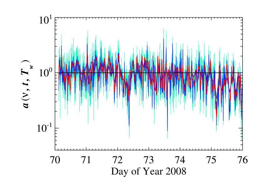
Figure 1.— Running power level, $a(\nu,t,T_{w})$, at frequency $\nu$ and with a time resolution $T_{w}$, as a function of time, $t$. The fast Fourier transforms were computed with a shifting window of width $T_{w}$ equal to the entire SW interval (black line), and $1/30$ (violet), $1/100$ (red), $1/300$ (blue), $1/900$ (light blue) of that interval duration for a frequency $\nu$ of $0.122\,$Hz. The running power level $a(\nu,t,T_{w})$ is smoothed on $200$ successive frequencies and normalized in this figure to the very long-time reference power level, $a_{\mbox{\scriptsize{ref}}}$.

3.2. Single-Frequency Multiple Time-Resolution Power-Level Fluctuations

Figure 1 shows the time variations of the power level $a(\nu,t,T_{w})$ computed at frequency $\nu\approx 0.122\,$Hz with a shifting window of width $T_{w}$ decreasing from $1/30$ the full duration of the SW stream (violet line) down to $1/900$ of it (light-blue line) by three successive factors of about $1/3$. The black line gives the very long-time reference power level, $a_{ref}$, to which the running power level $a$ is normalized. We see that the shorter the shifting window is, that is, the higher the time resolution of the spectral analysis is, the stronger the fluctuations of the power level are. The higher-resolution fluctuations far exceed the lower-resolution fluctuations, but roughly follow them in their time average, fractal-like. Figure 2 presents a zoom out of Figure 1, for the first day of data. The electronic version of Figure 1 can also be zoomed in to follow the four fluctuating lines and check how each is fluctuating around the line of next lower time resolution.

The power-level fluctuations of Figure 1 are smoothed on 200 successive frequencies. The effect of that smoothing is to reduce the amplitude of the fluctuations (see Figures 3 and 4 of Ragot 2013), especially at the lower values of power level, which can be most affected by noise. We checked that the effect of this reduction in fluctuation amplitude is to eliminate the tiny excess “bump” at the top of the PDFs of field variations presented in Figures 5$-$8 of Ragot (2013).

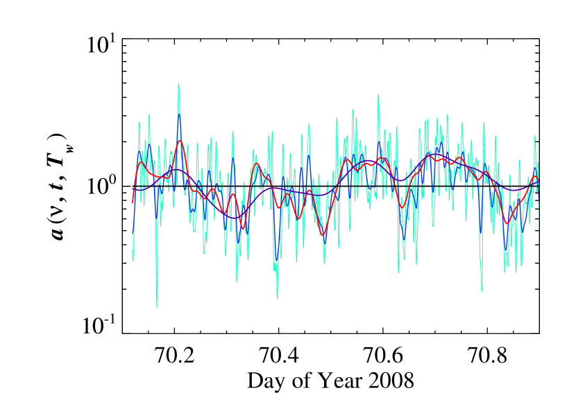
Figure 2.— Zoom out of Figure 1, day 70 of year 2008.

3.3. Multiple-Frequency Power-Level Fluctuations

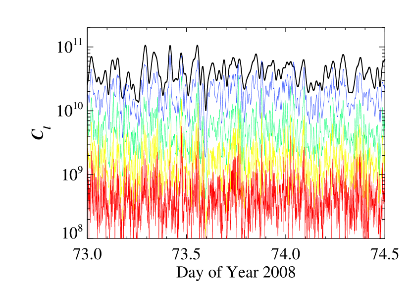
Figure 3.— Time variations of the spectral amplitudes $C_{l}\equiv a(\nu_{l},t,T_{w})\,V_{\mbox{{\small sw}}}\cos\phi_{r}$ of transverse magnetic field, from the lowest wavenumber (black line, $l=0$) to the “highest” (red line, $l=8$) by increments of 2. The amplitudes $C_{l}$ (up to $l=20$) are used to evaluate the turbulence level $\xi$ with Equations (LABEL:Dr), (9), (10) and (11).

When computing the power level at a given frequency $\nu$, the value of $\nu$ constrains the width $T_{w}$ of the window that can be used for the Fourier analysis. Typically, $T_{w}$ has to exceed a few times $\nu^{-1}$, and in order to capture the time variations of the power, $T_{w}$ must also be chosen as short as possible. Because the average slope of the turbulence spectrum appears to vary little with time (again, see Figure 2 of Ragot 2009 or Figure 4 of Ragot 2006d), and because our primary concern here is to capture the precise time variations of the power over a broad range of scales, we now compute the power at a higher frequency $\nu^{\prime}\approx 20\,\nu$ with a window of width $T_{w}=\nu^{-1}$, and extrapolate the result to the lower frequency $\nu$ by using the spectral slope obtained with a much longer window, covering the entire SW stream. Figure 3 shows the resulting time variations of the coefficients $C_{l}=C_{0}$, $C_{2}$, $C_{4}$, $C_{6}$ and $C_{8}$ in cm nT² [$a(\nu_{l},t,T_{w})=C_{l}/(V_{\mbox{{\small sw}}}\cos\phi_{r})$, see also Section 3.4] for the spectral amplitudes of transverse magnetic field, starting with the lowest wavenumber $k_{0}\approx 3.61\times 10^{-11}\,$cm (black line), where the turbulence spectrum becomes steeper than $k^{-1}$, and ending with $k_{8}\approx 7.55\times 10^{-10}\,$cm (red line).

For a wave vector ${\bf k}$ making an angle $\theta$ with the SW flow velocity, the wavenumber $k$ is related to the frequency $\nu$ through $k=2\pi\nu/(V_{\mbox{{\small sw}}}\cos\theta)$. Here we are considering a series of wave vectors ${\bf k}_{l}$ along the direction of the background magnetic field, that is, along the Parker spiral, and corresponding to a series of frequencies $\nu_{l}$. The flow velocity being practically radial in the SW, the wavenumbers $k_{l}$ are therefore related to the frequencies $\nu_{l}$ through $k_{l}=2\pi\nu_{l}/(V_{\mbox{{\small sw}}}\cos\phi_{r})$, with $\phi_{r}$ the angle of the Parker spiral to the radial direction at heliocentric distance $r$, as defined by Equation (2). The wavenumbers $k_{l}$ and wave vectors ${\bf k}_{l}$ are parallel wavenumbers and wave vectors along the Parker spiral, as needed for the modeling (see Sections 3.4 and 4), which calls for a one-dimensional projected spectrum along the background field [see also Equation (6) and following discussion].

As expected from Figures 1 and 2, in Figure 3 the time variations at the higher frequencies (or wavenumbers) roughly follow in their time average those of the lower frequencies, but locally display much more intense fluctuations. With the time-varying coefficients $C_{l}$, we can estimate in Section 3.4 the magnetic field-line mean cross-field displacement, $\langle(\Delta r)^{2}\rangle^{1/2}$, in the intermittent turbulence of the SW.

3.4. Mean Cross-Field Displacement
      in Intermittent Turbulence

The cross-field displacements $\Delta r$ on a background field-aligned scale $\Delta z$ are central to our study of magnetic field directions because in the turbulence of fast and slow SW streams on the scales $\Delta z\leq 10^{11}\,$cm, the ratios $\Delta r/\Delta z$ are expected to closely match (see introduction) the tangents of the angles $\alpha$ between the measured magnetic field, averaged on the corresponding timescale $\Delta t=\Delta z/(V_{\mbox{{\small sw}}}\cos\phi_{r})$, and the background field ${\bf B}_{0}$. That expectation of a close match between time-averaged field direction, obtained from in situ data, and direction of an actual field line is justified by our earlier study of field-line dispersal, which shows that on the scales $\Delta z\leq 10^{11}$cm in the SW, the cross-field displacements far exceed the variations in field-line separations (see, e.g., Ragot 2010b, and introduction). Again, this would not be the case if the field lines were too strongly diverging from each other.

The cross-field displacement $\Delta r$ is not defined from the data. However, it is a useful quantity whose root mean square, $\langle(\Delta r)^{2}\rangle^{1/2}$, the mean cross-field displacement, can be evaluated from the spectral amplitudes $C_{l}$ at wavenumber $k_{l}$ using predictions of the generalized quasilinear (GQL) theory (see below). $\langle(\Delta r)^{2}\rangle^{1/2}$ is central to our modeling. With $\langle(\Delta r)^{2}\rangle^{1/2}$, we can estimate in Section 4 the PDFs of the field-line directions, and compare them to the PDFs of the angles $\alpha$ between the time-averaged in situ fields and the background field ${\bf B}_{0}$.

The displacements $\Delta r$ of turbulent magnetic field lines across the direction of a background field ${\bf B}_{0}$ have been extensively studied for a general background field-aligned scale $\Delta z$ (Ragot 1999, 2006a, 2010a). The square root of their variance or mean cross-field displacement, $\langle(\Delta r)^{2}\rangle^{1/2}$, can be accurately estimated, both theoretically and numerically, in self-similar turbulence, that is, in a turbulence of single “constant-at-all-scales” spectrum of magnetic fluctuations. Both fully nonlinear and GQL estimates can be made for $\langle(\Delta r)^{2}\rangle^{1/2}$. On background field-aligned scales $\Delta z\leq 10^{11}\,$cm and for turbulence spectral shapes typical of slow or fast SW streams, nonlinear corrections to the GQL result in a background field ${\bf B}_{0}$

$$\langle(\Delta r)^{2}\rangle_{B_{0}} = {4\over B_{0}^{2}}\,\sum_{l}\left({C_{l}\over{(1-a^{\prime}_{l})k_{l}}}\right.$$

$$\times\left\{1-|k_{l}\Delta z|^{1-a^{\prime}_{l}}(1-a^{\prime}_{l})\,\Gamma(-1+a^{\prime}_{l})\sin\left({a^{\prime}_{l}\pi\over 2}\right)\right.$$

$$\left.-F_{P,Q}\left[\left\{{-1+a^{\prime}_{l}\over 2}\right\},\left\{{1\over 2},{1+a^{\prime}_{l}\over 2}\right\};{-(k_{l}\Delta z)^{2}\over 4}\right]\right\}$$

$$\hskip 39.83368pt-{C_{l+1}\over{(1-a^{\prime}_{l})k_{l+1}}}$$

$$\times\left\{1-|k_{l+1}\Delta z|^{1-a^{\prime}_{l}}(1-a^{\prime}_{l})\,\Gamma(-1+a^{\prime}_{l})\sin\left({a^{\prime}_{l}\pi\over 2}\right)\right.$$

$$\left.\left.-F_{P,Q}\left[\left\{{-1+a^{\prime}_{l}\over 2}\right\},\left\{{1\over 2},{1+a^{\prime}_{l}\over 2}\right\};{-(k_{l+1}\Delta z)^{2}\over 4}\right]\right\}\right)$$

of Ragot (1999, 2006a) [see also Equation (A13) of Ragot 2010a] are found to be negligible, even for much enhanced power levels (up to at least a factor of 40 at $10^{11}\,$cm, which would easily cover the range of enhancement values observed in Figures 1$-$3, and much more at shorter $\Delta z$ scales, see Ragot 2010a). On scales $\Delta z\leq 10^{11}\,$cm, accurate estimates of the mean cross-field displacement should therefore be obtained in the intermittent turbulence of the SW with the same GQL expression as given by Equation (LABEL:Dr), but with coefficients $C_{l}$ now varying with time and broadly departing from their long-time average value, as shown in Figure 3, rather than constant as in a self-similar turbulence. The expression of Equation (LABEL:Dr) should only remain valid, however, as long as strong variations of the amplitudes $C_{l}$ giving the dominant contribution do not occur on the timescales shorter than $\Delta t$, since constant amplitudes have been assumed on the corresponding lengthscale $\Delta z$ in the integration leading to Equation (LABEL:Dr). We return to that point in Section 4.

In Equation (LABEL:Dr), $C_{l}$ and $a^{\prime}_{l}$ are the amplitudes $C_{l}\equiv C_{\parallel}(k_{l})$ and spectral indexes of the one-dimensional or projected Fourier spectrum

$$C_{\parallel}(k_{\parallel})\equiv\int d{\bf k}_{\perp}\tilde{B}_{\perp}^{2}(k_{\parallel},{\bf k}_{\perp})$$ (6)

on the background field direction (parallel direction) at parallel wavenumbers $k_{\parallel}=k_{l}$, the assumption being that of a piecewise power-law spectrum with a well-defined single spectral index on each interval $[k_{l},k_{l+1}]$. In Equation (6), $\tilde{B}_{\perp}$ denotes the theoretical three-dimensional Fourier transform (with sliding window) of the transverse component of magnetic field.

Equation (LABEL:Dr) applies whatever the three-dimensional distribution of wavevectors, as long as it produces the projected spectrum of Equation (6). The SW measurements, however, give the spectrum projected on the SW flow direction rather than the background field. So the measured amplitudes $C_{l}$ of Figure 3 may not strictly coincide with the required $C_{\parallel}(k_{l})$, and the spectral indices $a^{\prime}_{l}$ used in our further estimates of $\langle(\Delta r)^{2}\rangle$ are not necessarily the spectral indexes of the projected Fourier spectrum of Equation (6). Only if the three-dimensional distribution of wavevectors is nearly isotropic (as found in slow SW by Narita et al. 2010 at the scale of $10^{9}\,$cm) should both sets of amplitudes and spectral indexes a priori coincide. The anisotropy found in the Cluster data analysis of Narita et al. (2010) becomes significant below the scale of $10^{9}\,$cm, with a $\sim\pm 50$ percent variation in the energy distribution from the parallel to the perpendicular directions at $4\times 10^{8}\,$cm, but these shorter turbulent scales do not contribute (or only very little) to the field-line displacements at the scales $\Delta z\sim 10^{9}\,$cm considered in this paper, nor to the mean cross-field displacements at any other scale. We therefore are hopeful that the discrepancy in the measurement direction of the one-dimensional spectra will not become an issue as we further make use of Equation (LABEL:Dr) in our analysis of Section 4.

In Equation (LABEL:Dr), $F_{P,Q}$ denotes the hypergeometric function, computed as a generalized hypergeometric series

$$F_{P,Q}[\{\alpha\},\{\beta,\eta\};\zeta] \equiv 1+{\alpha\,\zeta\over\beta\,\eta}+{\alpha(\alpha+1)\,\zeta^{2}\over\beta(\beta+1)\,\eta(\eta+1)\,2!}$$ (7)

$$+{\alpha(\alpha+1)(\alpha+2)\,\zeta^{3}\over\beta(\beta+1)(\beta+2)\,\eta(\eta+1)(\eta+2)\,3!}+\dots$$

(e.g., Gradshteyn & Ryzhik 1980) and $\Gamma$ is the Gamma function (Euler’s integral of the second kind) defined for $\mbox{Re}\,\alpha>0$ by the integral

$$\Gamma(\alpha)\equiv\int_{0}^{+\infty}dx\,e^{-x}x^{\alpha-1}\;.$$ (8)

The GQL result of Equation (LABEL:Dr) assumes a constant background field of magnitude $|B_{0}|$. However, the starting equation for the field-line tangent (see Equation (1) of Ragot 1999 or 2006a) calls for the actual $B_{z}$ field projection on the background ${\bf B}_{0}$, and provided that $B_{z}$ does not fluctuate too fast, or is averaged on a timescale long enough, it can obviously substitute for $B_{0}$ in Equation (LABEL:Dr). When there are significant long-scale fluctuations in the value of $B_{z}$, that substitution should greatly improve the estimate of the mean cross-field displacement. Therefore we write the mean cross-field displacement as

$$\langle(\Delta r)^{2}\rangle^{1/2}=\langle(\Delta r)^{2}\rangle^{1/2}_{B_{z_{\mbox{{\tiny av}}}}}\equiv{|B_{0}|\over|B_{z_{\mbox{{\tiny av}}}}|}\,\langle(\Delta r)^{2}\rangle^{1/2}_{B_{0}}\;,$$ (9)

where $\langle(\Delta r)^{2}\rangle_{B_{0}}$ is given by Equation (LABEL:Dr). Throughout the rest of this paper, unless otherwise specified, $\langle(\Delta r)^{2}\rangle^{1/2}$ denotes $\langle(\Delta r)^{2}\rangle^{1/2}_{B_{z_{\mbox{{\tiny av}}}}}$, the subscript $B_{z_{\mbox{{\tiny av}}}}$ of the medium-scale averaged $B_{z}$-field being omitted to lighten the notations. The background field $B_{0}$, or very long-time stream-average field, is computed for each of our fast SW streams by averaging the $B_{z}$-field over the entire stream. Shorter-scale fluctuations $\delta B_{z}$ of $B_{z}$ can be taken into account perturbatively in the evaluation of the mean cross-field displacement by expanding $[1+(\delta B_{z}/B_{0})^{2}]^{-1}$, which we later do to estimate the correction due to “compressibility effects.” An appropriate medium scale for averaging the background field and computing $B_{z_{\mbox{{\tiny av}}}}$ remains to be chosen. We return to the averaging scale of the local background field $B_{z_{\mbox{{\tiny av}}}}$ in Section 3.6.

3.5. Defining a Turbulence Level for the Time-Varying Intermittent Turbulence

From the multiple time-resolution and multiple-frequency Fourier spectral analysis of Sections 3.2 and 3.3, we realize that the “power level” of the intermittent SW turbulence is an extremely complex function of time and frequency, with wild fluctuations of large amplitude. In our study of the magnetic field orientations with varying turbulence level, we are therefore faced with a first serious challenge that consists in defining a turbulence level.

Our choice of a proper physical parameter that would both be a good representation of the level of turbulence at a given time and provide a good parametrization of the field orientations is guided here by our earlier theoretical and numerical studies of magnetic field-line wandering (Ragot 1999, 2006a, 2010). We know from these earlier studies that the displacements $\Delta r$ across the direction of the background field ${\bf B}_{0}$ on a given field-aligned scale $\Delta z$, which should give good estimates of the directions of the in situ magnetic fields averaged on the corresponding timescale $\Delta t=\Delta z/(V_{\mbox{{\small sw}}}\cos\phi_{r})$, is not dependent on the Fourier power level at just one frequency, but at a broad range of frequencies [see Section 3.4 and Equation (LABEL:Dr)]. Because the spectral power level is so wildly varying with time and frequency (see Figures 1–3), studying the field directions as functions of the spectral power level at any one single frequency may therefore not reveal the most meaningful trends of the data. By instead studying the field directions as functions of a linear combination of the Fourier power levels $C_{l}$ at a broad range of frequencies (or wavenumbers) that happen to produce the variance $\langle(\Delta r)^{2}\rangle$ of the field-line displacements [see Equations (LABEL:Dr) and (9)], we believe that we are optimizing our chances of uncovering the underlying organization of the field directions, and of modeling these field directions successfully.

The use of the mean cross-field displacement, $\langle(\Delta r)^{2}\rangle^{1/2}$, which is a linear combination of the spectral amplitudes $C_{l}$, rather than that of just one of the spectral amplitudes $C_{l}$, presents the advantage of incorporating the variability effects at all frequencies. Also, unlike the spectral amplitudes $C_{l}$, which may vary by up to a couple of orders of magnitude with time but actually tell us little about the turbulent behavior of the fields, the mean cross-field displacement has an obvious simple physical meaning that is directly related to the turbulent behavior of the fields. It is the quantity that we will be using here to quantify the turbulence level. More precisely, we introduce the parameter $C$ defined by

$$C^{1/2}\equiv{\langle(\Delta r)^{2}\rangle^{1/2}_{B_{z_{\mbox{{\tiny av}}}}}\over\Delta z}\;,$$ (10)

with the mean cross-field displacement $\langle(\Delta r)^{2}\rangle^{1/2}_{B_{z_{\mbox{{\tiny av}}}}}$ given by Equations (9) and (LABEL:Dr). The quantity $C^{1/2}$ is the mean cross-field displacement estimated with a background field magnitude equal to the average $|B_{z_{\mbox{{\tiny av}}}}|$ and divided by the field-aligned scale $\Delta z$. The parameter $C$ is a linear combination of the spectral amplitudes $C_{l}$ of magnetic field fluctuations [see Equation (LABEL:Dr)]. The product $C\,\Delta z$ is not a diffusion coefficient because the fields do not diffuse on the scales $\Delta z\leq 10^{11}\,$cm. Also, due to intermittency, $C$ strongly varies with time. A related parameter, which we will be abundantly using throughout this paper, is the angle

$$\xi\equiv\mbox{arctan}\left(C^{1/2}\right)\;.$$ (11)

Note that if the turbulence were self-similar with only one “constant-at-all-scales” spectrum of magnetic fluctuations, then $\langle(\Delta r)^{2}\rangle$ and $C$ would simply be proportional to any one of the amplitudes $C_{l}$, that is, to what is ordinarily understood as the energy level of turbulence in self-similar, non-intermittent turbulence. It is only because the SW turbulence is strongly intermittent that involving the mean cross-field displacement $\langle(\Delta r)^{2}\rangle^{1/2}$ in the definition of the turbulence level presents an advantage.

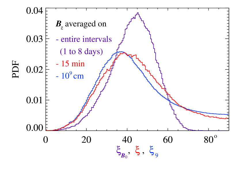
Figure 4.— PDFs of $\xi_{{}_{B_{0}}}\equiv\mbox{arctan}[\langle(\Delta r)^{2}\rangle^{1/2}_{B_{0}}/\Delta z]$ (violet), $\xi\equiv$ $\mbox{arctan}[\langle(\Delta r)^{2}\rangle^{1/2}_{B_{z_{\mbox{{\tiny av}}}}}/\Delta z]$ (red) and $\xi_{{}_{\huge 9}}\equiv\mbox{arctan}[(B_{0}/B_{z_{10^{9}\mbox{{\tiny cm}}}})$ $\langle(\Delta r)^{2}\rangle^{1/2}_{B_{0}}/\Delta z]$ (blue) for entire data set of fast SW streams. The long-time average field $B_{0}$ is computed for each individual SW stream (1 to 8 days in duration) while the average field $B_{z_{\mbox{{\tiny av}}}}$ is the running average over a timescale of $15\,$min.

3.6. Turbulence Level, $B_{z}$-Field Averaging Scale
and Field Reversals

An appropriate scale for computing the local average background field $B_{z_{\mbox{{\tiny av}}}}$ remains to be chosen. The PDFs of the turbulence-level parameter $\xi$, computed for a $B_{z}$ field averaged over each complete SW stream (violet), and over scales of $15\,$min (red) and $10^{9}\,$cm (blue), are presented in Figure 4 for our entire data set (121 intervals, 307.5 days). [The values of $\xi$ are computed from the $C_{l}$ amplitudes of Figure 3 using Equations (LABEL:Dr) and (9).] A complete SW stream is much too long (one to 8 days), while $10^{9}\,$cm, the scale over which we are computing the mean cross-field displacement, is too short. We find that an averaging scale of $15\,$min is a good compromise between the two. The PDFs of $\xi\equiv\xi_{15\,\mbox{{\small min}}}$ and $\xi_{9}\equiv\xi_{10^{9}\,\mbox{{\small cm}}}$ differ relatively little from each other, meaning that a $15\,$min average already captures most background field fluctuations. Also, a scale of $15\,$min in fast SW of speed exceeding $500-600\,$km s^-1 is a safe 40 to 50 times longer than the scale $\Delta z=10^{9}\,$cm. In the rest of this paper, unless otherwise specified, $B_{z_{\mbox{{\tiny av}}}}$ denotes the $15\,$min average of $B_{z}$.

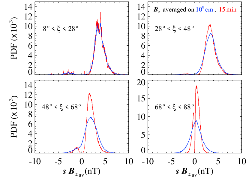
Figure 5.— PDFs of $sB_{z_{\mbox{{\tiny av}}}}$ for four intervals of turbulence levels ($8\arcdeg<\xi<28\arcdeg$, $28\arcdeg<\xi<48\arcdeg$, $48\arcdeg<\xi<68\arcdeg$ and $68\arcdeg<\xi<88\arcdeg$) and a $B_{z}$-field averaged on $10^{9}\,$cm (blue) and $15\,$min (red). $s$ is the sign of the background field polarization. The lower panels show an increasing rate of short-scale field reversals at increasing turbulence levels.

Figure 5 now compares the PDFs of $sB_{z_{\mbox{{\tiny av}}}}$, where $B_{z_{\mbox{{\tiny av}}}}$ is averaged on scales of $10^{9}\,$cm (blue) and $15\,$min (red), in four contiguous intervals of the parameter $\xi$ covering a total of 80°. The parameter $\xi$ is estimated with an averaging scale of $15\,$min for $B_{z_{\mbox{{\tiny av}}}}$ for both the blue and red PDFs. The polarization sign $s$ of the background field is computed from each complete SW stream. A negative value for $sB_{z_{\mbox{{\tiny av}}}}$ indicates a reversal of the field relative to the unperturbed Parker spiral field. While reversals are rare events at $\xi<48$°, they become relatively frequent at the higher values of $\xi$. At the highest levels of turbulence ($\xi>68$°, bottom-right panel of Figure 5), short-scale reversals are so frequent that on the shorter scale of $10^{9}\,$cm, reversed fields are practically as common as normal-polarity fields. This of course does not mean that field reversals are ubiquitous throughout the fast SW. The occurrence rate of $\xi>68\arcdeg$ is relatively low (see red curve in Figure 4). Still, it is far from negligible, and we find that if the unperturbed field is indeed along the Parker spiral direction, then field reversals are not rare occurrences in the fast SW. On the whole, again if the unperturbed field is along the Parker spiral direction, the field appears to be reversed between 4 and 10 percent of the time in fast SW streams. Note also that unlike for the $10^{9}$cm-average, the PDFs for the $15\,$min-average fall to zero at $sB_{z_{\mbox{{\tiny av}}}}=0$.

4. MODELING OF THE LOCAL-TO-BACKGROUND
FIELD ANGLES

From the mean cross-field displacement of Equations (LABEL:Dr) and (9), we can model the PDF of the angles $\alpha$ between local and background fields. As long as the GQL result holds, we expect Gaussian distributions for the displacements $\Delta x$ and $\Delta y$ in each of the directions perpendicular to the background field and a distribution,

$$f_{R}(\Delta r)={2\Delta r\over\langle(\Delta r)^{2}\rangle}e^{-(\Delta r)^{2}/\langle(\Delta r)^{2}\rangle}\;,$$ (12)

for the cross-field displacements $\Delta r\!=\![(\Delta x)^{2}+(\Delta y)^{2}]^{1/2}$. From this distribution, we derive in Section 4.2 of Ragot (2006b) the PDF,

$$f_{A}(\alpha)={\Delta z\over\cos^{2}\alpha}f_{R}\left[(\Delta z)\tan\alpha\right]\;,$$ (13)

for the angles $\alpha$ between local and background fields.

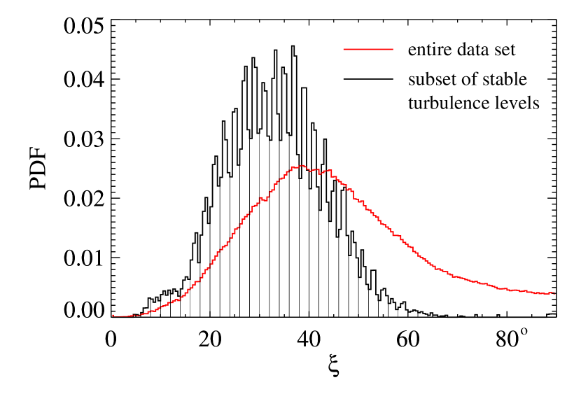
Figure 6.— PDFs of $\xi\equiv\mbox{arctan}[\langle(\Delta r)^{2}\rangle^{1/2}_{B_{z_{\mbox{{\tiny av}}}}}/\Delta z]$ for entire data set (red) and for a subset of time intervals over which the turbulence level, characterized by $\xi$, remains stable on a timescale of at least $400\,$s, that is, remains within the same 2°-wide bin over that timescale. The contributions from the highest turbulence levels are much reduced in the “stable” subset because the peaks of higher turbulence levels are usually of very short duration.

The GQL expression for the mean cross-field displacement in Equation (LABEL:Dr) assumes a turbulence spectrum that does not vary on the scale $\Delta z$ over which $\langle(\Delta r)^{2}\rangle$ is estimated. For a fixed value of the parameter $\langle(\Delta r)^{2}\rangle$, one should therefore expect our theoretical prediction to fit the observations only when the power level is stable on the scale $\Delta z$. From our large data set, we extract all the time intervals over which such conditions are satisfied. In Figure 6, we show the PDFs of the “power level” $\xi$ for both the entire data set (red) and the subset of time intervals over which the “power level” is stable, that is, the subset of time intervals over which $\xi$ remains within one 2°-wide bin for a time exceeding $400\,$s (which is slightly larger than $20\,\Delta z/V_{\mbox{{\small sw}}}$). The contribution from the highest turbulence levels are much reduced in Figure 6 in the “stable” subset because the peaks of higher power are usually of short duration or involve very steep time variations.

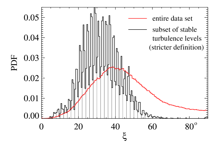
Figure 7.— Same as Figure 6, but for a stricter definition of the intervals of “stability,” wherein $150\,$s are removed at the ends of each subinterval. The contribution of each subinterval is now more peaked around its center.

Figure 7 shows similar PDFs for a stricter definition of stability whereby the edges of the stability intervals are removed (some $150\,$s on each end). This eliminates time intervals over which the computed turbulence power level may still be influenced by time intervals with different dominant power level. The contribution of each subinterval is now more peaked around its center, but the PDF shape is not otherwise significantly modified.

The purpose of these subsets of stable turbulence power levels is to check whether the angles between local and background fields can be accurately modeled and understood when the basic model requirement of stable turbulence levels is satisfied. For more generally varying turbulence power levels, the modeling would require a more complex convolution to include the contributions from all power levels. This is beyond the scope of the current paper. Here, we just want to find out whether the model has a chance to work in the first place and check the basics. We thus deconvolve the problem by decomposing the data into distinct turbulence power levels, instead of convolving the model.

On the $\Delta z$ scales less than $10^{11}$cm, the cross-field displacements far exceed the variations in field-line separations (see, e.g., Ragot 2010b). The cross-field displacements obtained by integrating the $B_{x}$ and $B_{y}$ measured in situ field components over time intervals of duration $\Delta t$ should therefore match the cross-field displacements of real magnetic field lines relatively well, and give good estimates of the actual angles $\alpha$ between local and background magnetic fields in the SW. Again, this would not be the case if the field lines were too strongly diverging from each other (see introduction, including footnotes).

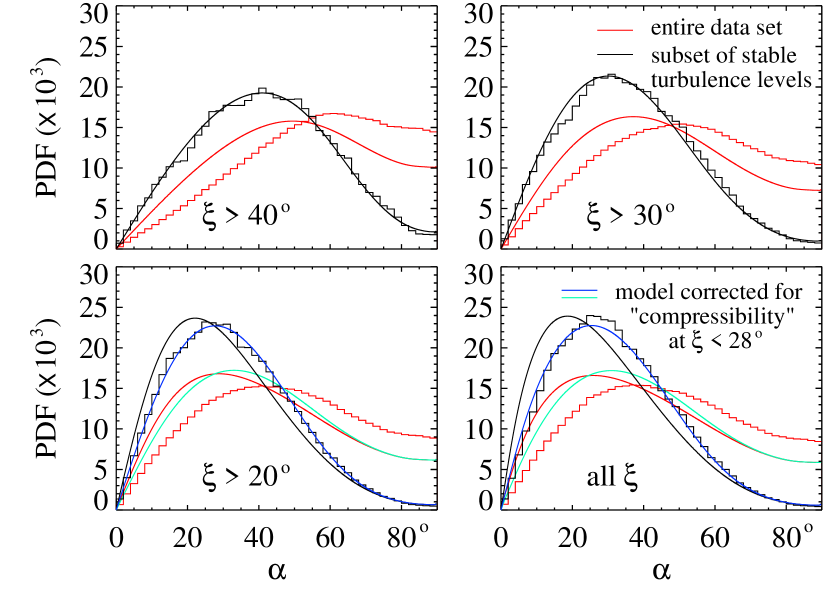
Figure 8.— Measured PDFs (histograms) and model PDFs (lines) of the angle $\alpha$ between local and background fields for entire data set (red) and for subset of stable turbulence levels (black) for turbulence levels $\xi>40\arcdeg$ (top-left panel), $\xi>30\arcdeg$ (top-right panel), $\xi>20\arcdeg$ (bottom-left panel) and all turbulence levels (bottom-right panel). The blue lines in the bottom panels are the model PDFs corrected for the measured “compressibility” of the turbulence. The model produces good fits for the subset of stable turbulence levels, but as expected, fails to fit the PDFs for the entire data set that includes intervals of fast varying turbulence level.

In Figure 8, we compare the model to the measured PDFs of the angle $\alpha$ between local and background magnetic fields (see footnote 8). The measured angles $\alpha$ are obtained from

$$\tan\alpha={\left\{\!\left[\sum_{-N/2}^{N/2}\!B_{x}(t\!+\!n\,\delta t)\right]^{2}\!\!\!\!+\!\left[\sum_{-N/2}^{N/2}\!B_{y}(t\!+\!n\,\delta t)\right]^{2}\!\right\}^{\!1/2}\over s\;\sum_{n=-N/2}^{N/2}B_{z}(t+n\,\delta t)}\,,$$ (14)

with the background field polarity sign, $s\equiv B_{0}/|B_{0}|$, for each sampling time $t$, excluding the first and last $N/2=\Delta t/(2\delta t)$ measurements of each SW stream (see also footnote 7). The value of $N$ slightly varies with time. It is given by the ratio of $\Delta z=10^{9}\,$cm over the local product $V_{\mbox{{\small sw}}}\,\delta t\,\cos\phi_{r}$ at time $t$. [If $N$ is an odd number, the sums are taken from $-(N-1)/2$ to $(N+1)/2$.] The PDFs computed from the entire data set are shown in red, while those computed for the subset of intervals with stable turbulence levels are shown in black. In each of the four panels, a different range of turbulence levels is included, from $\xi>40\arcdeg$ in the upper-left panel to all $\xi$ values in the lower-right panel. The reason for this distinction is that at the lowest values of $\xi$, typically below 28°, “compressive” field-aligned fluctuations become dominant. To the “non-compressive” transverse model based on Equation (LABEL:Dr), we then have to add a correction. This is done by expanding $[1+(\delta B_{z}/B_{0})^{2}]^{-1}$, and roughly results in the multiplication of the transverse result for $\langle(\Delta r)^{2}\rangle$ by a factor $1+3\langle(\delta B_{z}/B_{0})^{2}\rangle$. Numerically, it amounts to a factor of the order of $1.5$ in front of $B_{z_{\mbox{{\tiny av}}}}$. The results for the PDFs of $\alpha$ are the blue lines shown in the bottom panels of Figure 8.

The model (black lines in upper panels and dark-blue lines in bottom panels) fits the measured PDFs well for the subset of stable turbulence levels, confirming the validity of the model. As expected, however, the model does not fit the measured PDFs so accurately (see red and light-blue PDFs) when intervals of fast varying turbulence level are included in the data.

We now decompose the $\alpha$ PDFs into four ranges of turbulence levels ($8\arcdeg<\xi<28\arcdeg$ in violet, $28\arcdeg<\xi<48\arcdeg$ in green, $48\arcdeg<\xi<68\arcdeg$ in blue and $68\arcdeg<\xi<88\arcdeg$ in red). In Figure 9, we compare the PDFs of each subrange for the subset of stable turbulence levels and for the entire data set, both for a $B_{z}$-field averaged on $10^{9}\,$cm (top panel) and on $15\,$min [bottom panel, where the sum in the denominator of Equation (14) is made from -450 to 450 instead of -N/2 to N/2] in the definition of $\tan\alpha$. The measured $\alpha$ PDFs differ little at the lower turbulence levels, but more significantly at the higher levels.

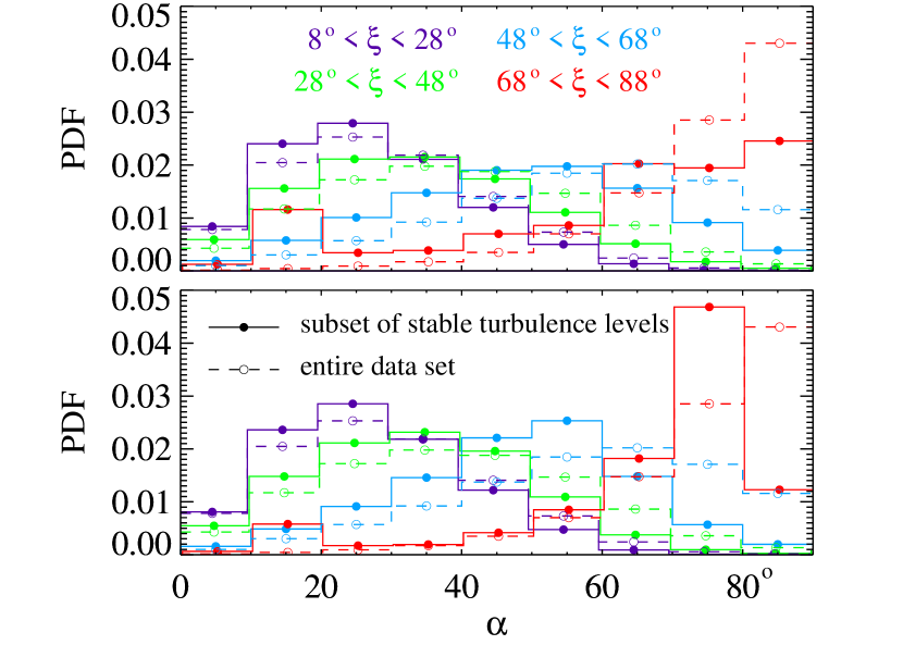
Figure 9.— Measured PDFs of $\alpha$ for entire data set (dashed-line histograms with empty circles) and for subset of stable turbulence levels (solid-line histograms with filled circles) decomposed into subintervals of turbulence levels, $8\arcdeg<\xi<28\arcdeg$ (violet), $28\arcdeg<\xi<48\arcdeg$ (green), $48\arcdeg<\xi<68\arcdeg$ (blue), $68\arcdeg<\xi<88\arcdeg$ (red), for $10^{9}\,$cm (top) and $15\,$min (bottom) averaged $B_{z}$ field in the definition of $\tan\alpha$.

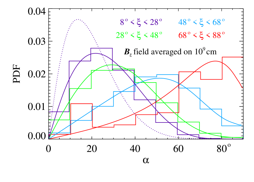
Figure 10.— Measured PDFs (histograms) and model PDFs (lines) of the angle $\alpha$ between local and background fields for subset of stable turbulence levels decomposed into four subintervals of turbulence levels, $8\arcdeg<\xi<28\arcdeg$ (violet), $28\arcdeg<\xi<48\arcdeg$ (green), $48\arcdeg<\xi<68\arcdeg$ (blue), $68\arcdeg<\xi<88\arcdeg$ (red), for $10^{9}\,$cm-averaged $B_{z}$ field. The violet dotted line shows the model PDF at low turbulence level prior to correction for “compressibility effect.”

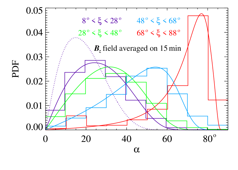
Figure 11.— Same as Fig. 10, but for a $15\,$min-averaged $B_{z}$ field.

With the same decomposition into four ranges of turbulence levels, we compare in Figure 10 the measured normalized $\alpha$ PDFs of the stable subset with the model PDFs. The statistics in the highest $\xi$-range are very limited and the error bars on the measured PDF very large. We therefore consider the model a reasonable fit in all four ranges of turbulence levels. While in Figure 10, the angles $\alpha$ are computed with a $B_{z}$-field averaged on $10^{9}\,$cm, in Figure 11 the $B_{z}$-field is averaged on a scale of $15\,$min in the denominator of Equation (14) (sum made from -450 to 450 instead of -N/2 to N/2). The comparison data/modeling remains satisfactory.

Figures 8, 10 and 11 reveal no problem with our modeling of the magnetic fields and of their orientations relative to the background field, as long as the turbulence level varies sufficiently slowly. On all subsets of stable turbulence level, we obtain fits of the measured PDFs that are actually quite good, even at the highest turbulence levels where the theory was not originally intended. Our GQL modeling and results do not assume anything about the turbulence isotropy or lack thereof. The only requirement for our turbulence model is that the three-dimensional distribution of wavevectors produces the right projected spectrum of turbulence [see Equation (6)]. So the positive result of our modeling actually supports an isotropic model of turbulence by not excluding it.

5. FROM $\alpha$ TO $\alpha_{r}$

Because the direction of the radial is known while that of the background field is in some measure assumed, the orientations of the SW magnetic fields are more often studied relative to the radial than to the background. Here, we go from the angles $\alpha$ relative to the background to the angles $\alpha_{r}$ relative to the radial, compare the PDFs of the two at a number of turbulence levels, and investigate how one goes from one to the other.

Returning to the entire data set, we show in Figure 12 the PDFs of field angles at a series of turbulence levels $\xi=11\pm 1$°, $\xi=31\pm 1$°, $\xi=51\pm 1$°, $\xi=71\pm 1$° and $\xi=89\pm 1$°. In Figure 12, only the central PDF at $\xi=51\pm 1$° is normalized. The other PDFs are given relative to that PDF and have much lower integrals at the lower and higher ends of the turbulence power levels. The PDFs of measured $\alpha$ angles between local and background fields are shown in dashed lines while the PDFs of measured $\alpha_{r}$ angles between local field and radial direction are shown in solid lines. The measured angles $\alpha_{r}$ are obtained from

$$\tan\alpha_{r}={\left\{\!\left[\sum_{\mbox{-}N/2}^{N/2}\!B_{T}(t\!+\!n\,\delta t)\right]^{2}\!\!\!\!+\!\left[\sum_{\mbox{-}N/2}^{N/2}\!B_{N}(t\!+\!n\,\delta t)\right]^{2}\!\right\}^{\!1/2}\over({B_{0_{R}}/|B_{0_{R}}|})\,\sum_{n=\mbox{-}N/2}^{N/2}B_{R}(t+n\,\delta t)}\,,$$ (15)

where $B_{R}$, $B_{T}$ and $B_{N}$ are the measured magnetic field components in the RTN coordinate system ($R$: along the radial, pointing away from the Sun; $T$: orthoradial in the ecliptic, pointing west; $N$: normal to the ecliptic, pointing north). $B_{0_{R}}$ is the R-component of the very long-time, stream-average field, the ratio $B_{0_{R}}/|B_{0_{R}}|$ giving again the field polarity in each SW stream.

To test our understanding of the measured fields and a couple of simple hypotheses, we now use the PDFs of measured $\alpha$ to simulate the angles $\alpha_{r}$ and their PDFs. Through Monte-Carlo simulation, we generate sets of $\alpha$ angles with the measured PDFs. Assuming (1) a background field along the Parker spiral direction and (2) axisymmetry of the turbulent fields around that background field, we then transform the angles $\alpha$ into the angles $\alpha_{r}$ between local field and radial direction. Finally, we compute the PDFs of these new angles and show them in dotted lines in Figure 12. The modeled PDFs of $\alpha_{r}$ appear to fit the measured PDFs reasonably well as soon as $\xi>26\arcdeg$. At the highest turbulence levels, above $\xi\approx 60\arcdeg$, we note that the $\alpha_{r}$ PDFs, both measured and modeled, are nearly flat on a broad range of angles $\alpha_{r}$ between $50-60\arcdeg$ and $110-120\arcdeg$. This we now believe can be attributed to the broad and nearly axisymmetric distribution of the turbulent fields about the background-field direction.

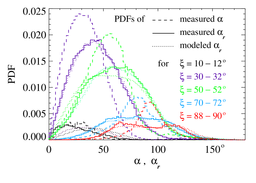
Figure 12.— PDFs of measured $\alpha$ angles between local and background fields (dashed lines) and of measured and modeled $\alpha_{r}$ angles between local field and radial direction (solid and dotted lines, respectively) for a series of turbulence levels $\xi=11\pm 1$°, $\xi=31\pm 1$°, $\xi=51\pm 1$°, $\xi=71\pm 1$° and $\xi=89\pm 1$°. The green PDFs for $\xi=51\pm 1$° are normalized and serve as reference level for the other “PDFs.” The model PDFs are obtained from the measured $\alpha$ PDFs by Monte-Carlo simulations assuming axisymmetry of the local field directions relative to the background. The dotted lines of matching color are obtained for a background field along the Parker spiral. The two additional dotted lines (green-blue for $\xi=51\pm 1$° and dark-violet for $\xi=11\pm 1$°) are computed for a background field at 7° and 8° to the Parker spiral, respectively, slightly improving the fit to the measured PDFs.

In the cases $\xi=50\pm 1\arcdeg$ and $\xi=10\pm 1\arcdeg$, where the modeled PDFs are less than satisfactory, we do an additional transformation with a slightly different background field direction, shifted by some 7 and 8° relative to the Parker spiral. The results are also shown in dotted lines, but with a slightly different color. They appear to improve the fit to the measured PDFs of $\alpha_{r}$, but the fit at the lowest turbulence level remains less than satisfactory. The issue there again might be connected to the measured “compressibility” of the turbulence.

We also note that the statistics in the central power bin ($\xi=51\pm 1\arcdeg$) are relatively high, and that a large number of SW streams contribute to these statistics, with a spread in the Parker spiral direction of more than 4 degrees around the mean value of $\phi_{r}\approx 34\arcdeg$. It may be affecting our result, but reduced statistics with more constrained values of $V_{\mbox{{\small sw}}}$ and therefore $\phi_{r}$ did not seem to change that result. This issue will need further investigation.

From the simple test of this section, we conclude that axisymmetry of the turbulent fields around a background field in or near the direction of the Parker spiral is a reasonably good assumption that produces fairly accurate fits of the measured PDFs of $\alpha_{r}$ angles, away from the lowest turbulence levels where $B_{z}$ turbulence becomes dominant, that is, above $\xi\approx 26\arcdeg$. This “axisymmetry” result appears to us difficult to reconcile with an $\alpha_{r}$ anisotropy of turbulence power driven by a wavevector anisotropy.

6. CONSEQUENCES OF THE TURBULENCE-LEVEL
VARIABILITY ON FIELD ORIENTATIONS
AND APPARENT ANISOTROPY

Figure 13 displays the PDFs of “turbulence levels” $\xi$ for series of angles $\alpha$ (left panels) and $\alpha_{r}$ (right panels) measured between 0 and 90° (top panels) and between 0 and 180° (bottom panels). The left panels show PDFs peaking at the highest levels of turbulence near the normal to the background field (green PDF), and at the lowest levels near the direction of the background field (black, yellow), with a clear shifting of the peak with the angles $\alpha$ and $\alpha_{90}$. Magnetic fields near the normal to the background dominate at the highest levels of turbulence, while magnetic fields close to the background field direction dominate at the lowest turbulence levels $\xi$, which can also be seen in Figure 12 (see also dashed-line histograms for entire data set of Figure 9). As a consequence, because the angle between background and radial direction is relatively small in fast SW ($\sim 30\arcdeg$), it is also true that magnetic fields at large angles to the radial are preponderant at higher $\xi$, while magnetic fields closer to the radial are more frequent at lower $\xi$. But the effect is less striking in the right panels of Figure 13 than that for the angles $\alpha$ relative to the background in the left panels.

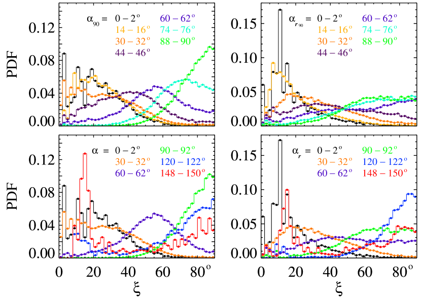
Figure 13.— Measured PDFs of turbulence levels $\xi$ for series of intervals of angles between local and background fields, $\alpha_{90}$ and $\alpha$ (left panels), and between local field and radial, $\alpha_{r_{90}}$ and $\alpha_{r}$ (right panels). The angles $\alpha$ and $\alpha_{r}$ are measured between 0 and 180°, while the angles with an index 90 are measured between 0 and 90°. The left panels show PDFs peaking at the highest levels of turbulence near the normal to the background field (green PDF), and at the lowest levels near the direction of the background field (black, yellow), with a clear shifting of the peak with the angles $\alpha$ and $\alpha_{90}$.

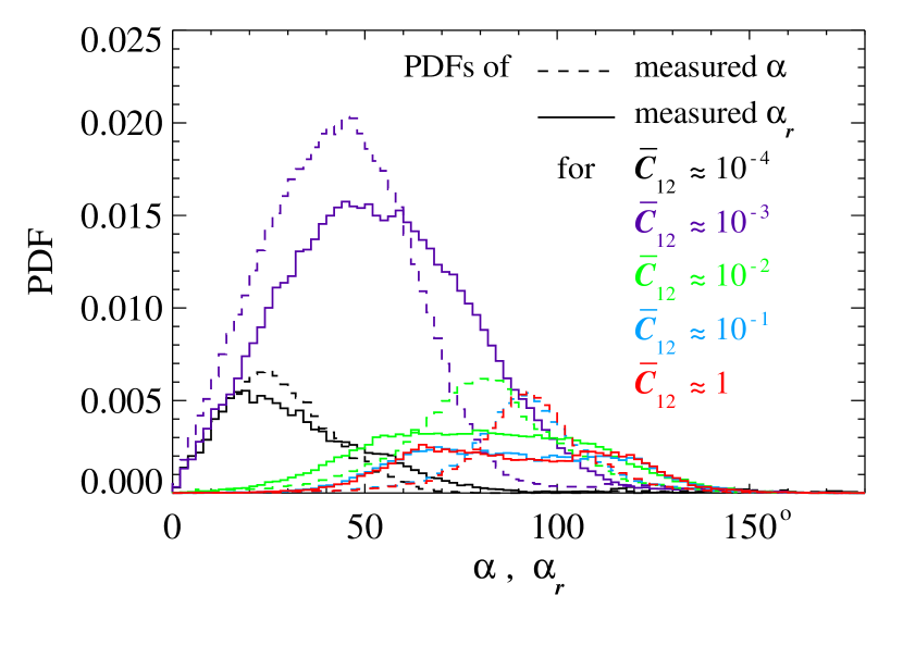
Figure 14.— “Same as” Figure 12, but for a turbulence level defined as $C_{12}/(B_{z_{\mbox{{\tiny av}}}}^{2}\Delta z)$ (i.e., from the fluctuations at a single frequency $\nu\approx 0.028\,$Hz) instead of $\langle(\Delta r)^{2}\rangle_{B_{z_{\mbox{{\tiny av}}}}}/(\Delta z)^{2}$, which depends on a broad range of frequencies. The parameter $\overline{C}_{12}$ is $C_{12}/(2B_{z_{\mbox{{\tiny av}}}}^{2}\Delta z)$ and the PDFs are computed for the values of $\overline{C}_{12}$ giving, for $n=4$, 3, 2, 1 and 0, a $\xi_{12}\equiv\arctan[20(2\overline{C}_{12})^{1/2}]$ within a $2\arcdeg$ bin containing $\arctan(20\times 2^{1/2}\times 10^{-n/2})$ (the bins all start at multiples of $2\arcdeg$). The violet PDFs for $\overline{C}_{12}=10^{-3}$ are normalized and serve as reference level for the other “PDFs.”

The strong “anisotropy” shown in Figures 12 and 13, and further in Figure 17, of course is related to our choice of the parameter $\xi$ to characterize the turbulence level [see Equations (10–11)]. This parameter closely orders the peaks of the $\alpha$ and $\alpha_{90}$ PDFs because it is related to the mean cross-field displacement of the turbulent field lines. But we argue that the power level has to be divided by the squared magnitude of the background magnetic field, as it is done in the definition of $C$ and therefore $\xi$, because in itself, the power in $\delta B$ tells us nothing about turbulence; it is the power in $\delta b\equiv\delta B/B_{z_{\mbox{{\tiny av}}}}$ (of the fluctuations relative to the background) that does. No matter how high the power in $\delta B$, if $B_{z_{\mbox{{\tiny av}}}}$ is high enough, it will “quench” the turbulence.

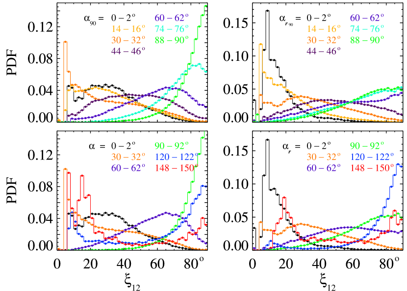
Figure 15.— “Same as” Figure 13, but for a turbulence level defined as $C_{12}/(B_{z_{\mbox{{\tiny av}}}}^{2}\Delta z)$ instead of $\langle(\Delta r)^{2}\rangle_{B_{z_{\mbox{{\tiny av}}}}}/(\Delta z)^{2}$. The parameter $\xi_{12}$ is $\arctan[20\,(C_{12}/\Delta z)^{1/2}/B_{z_{\mbox{{\tiny av}}}}]$.

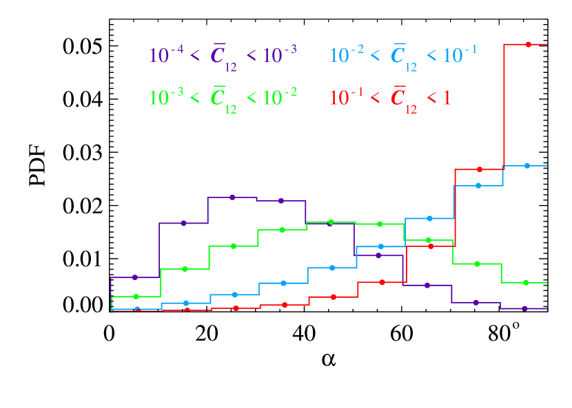
Figure 16.— Same as dotted-line histograms of the top panel of Figure 9, but for a turbulence level defined as $C_{12}/(B_{z_{\mbox{{\tiny av}}}}^{2}\Delta z)$. The
parameter $\overline{C}_{12}$ is one half that turbulence level. Again, the highest turbulence levels are found near the normal to the Parker spiral and the lowest levels near the Parker spiral direction.

Figures 14 and 15 are the “equivalent” of Figures 12 and 13 with a turbulence level defined using the field fluctuations $C_{12}/B_{z_{\mbox{{\tiny av}}}}^{2}$ at only one frequency (close to $V_{\mbox{{\small sw}}}/\Delta z$), rather than using the mean cross-field displacement $\langle(\Delta r)^{2}\rangle^{1/2}_{B_{z_{\mbox{{\tiny av}}}}}$ as in Section 3.5. Similar conclusions can be drawn from these figures. So our conclusion that the highest turbulence levels are found near the normal to the Parker spiral and the lowest levels near the Parker spiral direction is not due to the use of $\langle(\Delta r)^{2}\rangle_{B_{z_{\mbox{{\tiny av}}}}}/(\Delta z)$ in place of $C_{12}/B_{z_{\mbox{{\tiny av}}}}^{2}$ in the definition of the turbulence level. Figure 16 also shows the PDFs of the angles $\alpha$ for a series of intervals of the parameter $\overline{C}_{12}\equiv C_{12}/(2B_{z_{\mbox{{\tiny av}}}}^{2}\Delta z)$. The PDFs of Figure 16 are to be compared to the dashed-line histograms of the top panel of Figure 9 for the entire data set. Again, the results are similar whether the definition of the turbulence level involves $\langle(\Delta r)^{2}\rangle_{B_{z_{\mbox{{\tiny av}}}}}/(\Delta z)$ or only $C_{12}/B_{z_{\mbox{{\tiny av}}}}^{2}$.

We note, however, that the parameter $\xi\equiv\arctan$ $(\langle(\Delta r)^{2}\rangle^{1/2}_{B_{z_{\mbox{{\tiny av}}}}}/\Delta z)$ used throughout this paper is a more meaningful ordering parameter because the turbulent magnetic field lines are affected by the turbulent field fluctuations at a broad range of frequencies, down to where the spectrum becomes flatter than $k^{-1}$, and not just by the fluctuations at the frequency inverse of the averaging timescale for the computation of the mean local field direction. The parameter $\xi$, in all instances where the transverse fluctuations dominate, that is, above about $26\arcdeg$, gives the approximate location of the peak in the PDFs of the angles $\alpha$ between mean local and background Parker fields.

Figure 17.— Average turbulence levels $C_{\mbox{{\small av}}}\equiv\int_{0^{o}}^{84^{o}}\!\!d\xi\,P(\xi,\alpha)\tan^{2}\xi$,
where $\tan\xi\equiv\langle(\Delta r)^{2}\rangle^{1/2}_{B_{z_{\mbox{{\tiny av}}}}}/\Delta z$, relative to their value at the lowest
angle $\delta\alpha/2=1$°, as functions of the angle $\alpha$  (filled  black  circles),
$\alpha_{90}\!$ (empty red circles), $\alpha_{r}\!$ (black squares) and $\alpha_{r_{90}}\!\!$ (blue triangles).

Knowing the bivariate PDFs $P(\xi,\alpha^{\prime})$ for $\alpha^{\prime}=\alpha$, $\alpha_{90}$, $\alpha_{r}$ and $\alpha_{r_{90}}$, we can now estimate the average turbulence level at each angle $\alpha^{\prime}$ by computing the integral

$$C_{\mbox{{\small av}}}(\alpha^{\prime})\equiv\int_{0{\tiny\arcdeg}}^{\xi_{\mbox{{\tiny max}}}}d\xi\,P(\xi,\alpha^{\prime})\tan^{2}\xi\;,$$ (16)

with a cutoff at $\xi=\xi_{\mbox{{\small max}}}$. The results relative to $C_{\mbox{{\small av}}}(\delta\alpha/2)$ in the first bin of the $\alpha^{\prime}$ histograms, are presented in Figure 17 for $\xi_{\mbox{{\small max}}}=84\arcdeg$. The peaks’ heights are very sensitive to the value of the cutoff $\xi_{\mbox{{\small max}}}$. For instance, a value $\xi_{\mbox{{\small max}}}=88\arcdeg$ would produce a peak in $\alpha\approx 100\arcdeg$ over 4 times higher than found here in Figure 17, and if all turbulence levels present in our data set were included, that peak would exceed 500. The value $\xi_{\mbox{{\small max}}}=84\arcdeg$ was chosen because it is already sufficiently large to produce high peaks, yet still low enough to keep the rising phase of the curves at low $\alpha^{\prime}$ clear.

Most importantly, we note that the ratio $C_{\mbox{{\small av}}}(89\arcdeg)/C_{\mbox{{\small av}}}(1\arcdeg)$ is much greater for $\alpha$ and $\alpha_{90}$ than it is for $\alpha_{r}$ and $\alpha_{r_{90}}$. The dependence on $\alpha$ of the turbulence level is the main effect, that of the turbulence level on $\alpha_{r}$ a mere consequence of it. The steeper dependence on $\alpha$, or stronger “anisotropy” in $\alpha$, is due to the fact that the $\alpha$ PDFs remain peaked at all turbulence levels $\xi$, whereas the $\alpha_{r}$ PDFs become flat at the higher $\xi$ (see Figure 12) as a result of the broad and presumably nearly axisymmetric distribution of field directions about the background field direction.

Figure 18.— Same as Figure 17, but with “$\tan\xi$” defined as $(C_{12}/\Delta z)^{1/2}/|B_{z_{\mbox{{\tiny av}}}}|$ rather than $\langle(\Delta r)^{2}\rangle^{1/2}_{B_{z_{\mbox{{\tiny av}}}}}/\Delta z$. The coefficient $C_{12}$ corresponds to a frequency $\nu\approx 0.028\,$Hz.

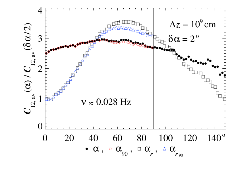
Figure 19.— Same as Figure 18, but with the long-time average $B_{0}$ substituting for the $15\,$min average $B_{z_{\mbox{{\tiny av}}}}$. Also, all $C_{12,\mbox{{\small av}}}$ are normalized to the same value of $C_{12,\mbox{{\small av}}}(\theta_{r})$ at $1\arcdeg$ rather than their own value at $1\arcdeg$.

Also, the use of the amplitudes $C_{l}/(B_{z_{\mbox{{\tiny av}}}}^{2}\Delta z)$ rather than $C$ as defined in Equation (10) would lead to much steeper curves and higher peaks, depending on the frequency (see Figure 18). The higher the frequency, the higher the peaks, consistent with the findings of Podesta (2009). Finally, when the running $15\,$min average $B_{z_{\mbox{{\tiny av}}}}$ of the background field magnitude is replaced by the long-time average $B_{0}$ in the definition of $\xi$, the sharp dependence of the average turbulence level $C_{12,\mbox{{\small av}}}$ on the angles $\alpha$ and $\alpha_{r}$ is damped out. It is reduced in Figure 19 to a mere factor $3-3.5$ increase in $\alpha_{r}$, and is almost entirely suppressed in $\alpha$. The result of Figure 19 for the dependence on $\alpha_{r}$ is very much consistent with the results shown in the top panel of Figure 7 in Podesta (2009).

The strong “anisotropy” presented in this section is in no way related to any anisotropy in the wavevector distribution of the turbulence. The fact that the turbulence levels are observed to be much higher in the directions close to the normal to the Parker spiral than in the directions close to the Parker spiral itself is strictly due to the facts that (1) the field directions deviate more strongly from the Parker spiral direction when the turbulence is higher, and (2) the turbulence level varies strongly with time, enabling the observation of a wide range of field directions and turbulence levels. So the strong apparent “anisotropy” presented in this section is strictly a consequence of the turbulence-level time variability.

7. CONCLUSION

In an effort to identify the effects of the broad variations in turbulence levels on the orientations of the local mean fields, we have analyzed the turbulent magnetic fields of a large set of fast SW streams measured onboard ACE and STEREO A and B. Our multiscale Fourier analysis of the transverse turbulent fields reveals time variations of the spectral power at all frequencies and on many timescales. The higher the time resolution of the spectral analysis is, the stronger the fluctuations of the power level are. The higher-resolution fluctuations far exceed the lower-resolution fluctuations, but roughly follow them in their time average (see Figures 1$-$3). From this multiscale Fourier analysis, we estimate as a linear combination of the Fourier amplitudes $C_{l}$ (see Figure 3) the GQL mean cross-field displacement of the magnetic field lines in the time-varying intermittent turbulence. This estimate of the mean cross-field displacement in intermittent turbulence is given by the square root of Equation (LABEL:Dr) with a local medium-scale ($\sim 15\,$min) average background field $B_{z_{\mbox{{\tiny av}}}}$ substituting for the stream average $B_{0}$. It includes the effects of all turbulent scales and fluctuates on many timescales. This estimate of the mean cross-field displacement, once divided by the field-aligned scale $\Delta z$, defines the square root $C^{1/2}$ of the power level of the intermittent turbulence in Equation (10), and the related angle, $\xi\equiv\arctan C^{1/2}$, used throughout the paper to parametrize the power level of the intermittent turbulence.

Provided “compressibility effects” are included at the lowest power levels of turbulence ($\xi<26\arcdeg$), modeling the PDFs of the angles $\alpha$ between local and background fields produces satisfactory fits of the observed PDFs at all stable power levels of turbulence (see Figures 8, 10 and 11), that is, on all time intervals with variations in the power level of turbulence that are sufficiently slow. Because the highest power levels of turbulence happen in short bursts, the statistics for stable power levels are biased toward the lower turbulence levels and smaller angles (see Figures 6$-$9). But the fits remain quite accurate at all levels $\xi$, even for the very low statistics of the higher $\xi$. Because our GQL modeling does not assume anything about the three-dimensional distribution of wavevectors in the turbulence, and therefore does not preclude an isotropic distribution of wavevectors, it follows from these fits that an isotropic turbulence could account for the measured PDFs of the angles $\alpha$ between local and background fields at all stable levels of turbulence.

Both the direct measure of the field projection on the background field (Parker spiral direction) and the PDFs of the measured angles $\alpha$ between local and background fields reveal local field reversals that are quite common even within very broad streams of “unipolar” fast SW (see Figures 5 and 12). On the whole, they happen some 4 to 10 percent of the time, but at the highest levels of turbulence, short-scale reversals are so frequent that on the scale of $10^{9}\,$cm, reversed fields are practically as common as normal-polarity fields.

Modeling through Monte-Carlo simulation the PDFs of the angles $\alpha_{r}$ between local fields and radial direction from the measured PDFs of the angles $\alpha$, we find that axisymmetry of the turbulent fields around a background field in or near the direction of the Parker spiral is a reasonably good assumption. The modeling made under this simple assumption does indeed produce fairly accurate fits of the measured PDFs of $\alpha_{r}$ angles, away from the lowest turbulence levels where $B_{z}$ fluctuations become dominant, that is, above $\xi\approx 26\arcdeg$. At the highest turbulence levels, above $\xi=60\arcdeg$, both the model and observed $\alpha_{r}$ PDFs are nearly flat on a broad range of angles $\alpha_{r}$ between $50-60\arcdeg$ and $110-120\arcdeg$ (see Figure 12).

Unsurprisingly, magnetic fields near the normal to the background field or Parker spiral dominate at the highest turbulence levels, while magnetic fields close to the Parker spiral direction dominate at the lowest turbulence levels $\xi$, with a peak of the $\alpha$ ($\xi$) angle PDFs smoothly shifting from the parallel to the normal direction (from the low to the high turbulence levels) as $\xi$ ($\alpha$) increases [Figure 12 (13)]. This results in a very steep dependence of the average power level of turbulence $C_{\mbox{{\small av}}}$ of Equation (16) on the angle to the Parker spiral, and in a more moderate dependence on the angle to the radial (Figure 17). The steeper dependence on $\alpha$ is due to the fact that the $\alpha$ PDFs remain peaked at all $\xi$ whereas the $\alpha_{r}$ PDFs, due to the broad and nearly axisymmetric PDFs of the field directions relative to the background, become flat at the higher $\xi$. The dependence is found to be even steeper for the higher-frequency amplitudes $C_{12,\mbox{{\small av}}}/B_{z_{\mbox{{\tiny av}}}}^{2}$ (Figure 18), but strongly reduced for $C_{12,\mbox{{\small av}}}$ (Figure 19). Our conclusion that magnetic fields near the normal to the background Parker spiral dominate at the highest turbulence levels, while magnetic fields close to the Parker spiral direction dominate at the lowest turbulence levels is not modified by the use of a single-frequency turbulence-level definition $C_{12}/(B_{z_{\mbox{{\tiny av}}}}^{2}\Delta z)$ in the place of $\langle(\Delta r)^{2}\rangle_{B_{z_{\mbox{{\tiny av}}}}}/(\Delta z)^{2}$ (Figures 14–16).

We do not presume to know whether the $\alpha_{r}$ “anisotropy” of $C_{12,\mbox{{\small av}}}$ presented in Figure 19 is a residual effect of the strong variability in the power level of turbulence. But we can certainly conclude that the extreme “anisotropy” seen in Figures 17 and 18 is unambiguously caused by the time variability in that power level of turbulence, and not by any anisotropy in the wavevector distribution of the turbulence. Clearly, a purely isotropic model of turbulence, that is, a model of turbulence with an isotropic distribution of wavevectors ${\bf k}$, can reproduce the PDFs of the angles $\alpha$ and $\alpha_{r}$ between local and background fields and between local field and radial direction presented in this paper for series of the power level of turbulence. By this we mean that an isotropic model of turbulence cannot be excluded on the basis of the observed dependences of the angle PDFs on the power level of turbulence, or of the average power levels of turbulence on the angles. These dependences are entirely imputable to the time variability in the power level of turbulence observed in the fast SW streams. These results are consistent with the near isotropy found by Narita et al. (2010) from four-point magnetic field measurements of the Cluster spacecraft at the turbulence scales close to $10^{9}\,$cm in the SW.

The parameter $\xi$ defined by Equations (10) and (11) does order the directions of the local fields best because it physically represents the local statistical average directions. This tight ordering of the local field directions with the parameter $\xi$ brings the observed “anisotropies” of the average power level of turbulence to extremes much higher than otherwise found with the power level undivided by the local background field. But again, we argue that the power level has to be divided by the squared magnitude of the background magnetic field because in itself, the power in $\delta B$ tells us nothing about turbulence, it is the power in $\delta b\equiv\delta B/B_{z_{\mbox{{\tiny av}}}}$ that does. No matter how high the power in $\delta B$, if $B_{z_{\mbox{{\tiny av}}}}$ is high enough, it will “quench” the turbulence.

The variations of $B_{z_{\mbox{{\tiny av}}}}$ itself are likely caused, in large part, by the non-uniformity of the emerging fields within each of the coronal holes at the source of the fast SW streams. We suggest that some of the variations of $B_{z_{\mbox{{\tiny av}}}}$, in particular the local field reversals (Figure 5; Section 3.6), may also be signs of intermixed magnetic fields of opposite polarity, originating from a different SW stream, perhaps even signs of ongoing reconnection with these opposite-polarity fields, or remnants of reconnections that took place earlier. Though it is of course also possible and even likely that some of these local field reversals are due to the reconnection, at the basis of the corona, within coronal holes, of open field lines with closed magnetic loops.

References

- Burlaga (1995) Burlaga, L. F. 1995, Interplanetary Magnetohydrodynamics (Oxford University Press)
- Burlaga (1997) Burlaga, L. F., & Ness, N. F. 1997, J. Geophys. Res., 102, 19731
- Daubechies (1992) Daubechies, I. 1992, Ten Lectures on Wavelets (Philadelphia: SIAM)
- GradshteynRyzhik (1980) Gradshteyn, I. S., & Ryzhik, I. M. 1980, Table of Integrals, Series and Products (New York: Academic Press)
- Hirschberg (1969) Hirshberg, J. 1969, J. Geophys. Res., 74, 5841
- NGSG (2010) Narita, Y., Glassmeier, K.-H., Sahraoui, F., & Goldstein, M. L. 2010, Phys. Rev. Lett., 104, 171101
- NessWilcox (1966) Ness, N. F., & Wilcox, J. M. 1966, ApJ, 143, 23
- Parker (1958) Parker, E. N. 1958, ApJ, 128, 664
- Parker (1963) Parker, E. N. 1963, Interplanetary Dynamical Processes (Wiley-Interscience, New York)
- Podesta (2009) Podesta, J. J. 2009, ApJ, 698, 986
- Ragpt (1999) Ragot, B. R. 1999, ApJ, 525, 524
- Ragot (2006a) Ragot, B. R. 2006a, ApJ, 645, 1169
- Ragot (2006b) Ragot, B. R. 2006b, ApJ, 651, 1209
- Ragot (2009) Ragot, B. R. 2009, ApJ, 690, 619
- Ragot (2010a) Ragot, B. R. 2010a, ApJ, 715, 959
- Ragot (2010b) Ragot, B. R. 2010b, ApJ, 723, 1787
- Ragot (2011) Ragot, B. R. 2011, ApJ, 740, 119
- Ragot (2013) Ragot, B. R. 2013, ApJ, 765, 97