Closed String Thermodynamics and a Blue Tensor Spectrum
Abstract
The BICEP-2 team has reported the detection of primordial cosmic microwave background B-mode polarization, with hints of a suppression of power at large angular scales relative to smaller scales. Provided that the B-mode polarization is due to primordial gravitational waves, this might imply a blue tilt of the primordial gravitational wave spectrum. Such a tilt would be incompatible with standard inflationary models, although it was predicted some years ago in the context of a mechanism that thermally generates the primordial perturbations through a Hagedorn phase of string cosmology. The purpose of this note is to encourage greater scrutiny of the data with priors informed by a model that is immediately falsifiable, but which predicts features that might be favoured by the data– namely a blue tensor tilt with an induced and complimentary red tilt to the scalar spectrum, with a naturally large tensor to scalar ratio that relates to both.
pacs:
98.80.CqI Introduction
The BICEP-2 team just announced the detection of primordial cosmic microwave background (CMB) B-mode polarization, implying a tensor-to-scalar ratio of BICEP . The positive detection of primordial gravitational waves constitutes a major advance for early universe cosmology, giving us a new diagnostic tool with which to scrutinize models of the very early universe against observational data. Conventional adiabatic cosmological fluctuations do not predict any B-mode polarization at the linear level in cosmological perturbation theory. Hence in the context of the simplest models, primordial B-mode polarization must be due to gravitational waves 111Note, however, that beyond the simplest single field scalar models, there are other sources of B-mode polarization e.g. from cosmic strings Holder . B-mode polarization will also be produced by lensing of E-mode polarization, which in turn is directly generated from cosmological fluctuations, and that this B-mode lensing signal has in fact recently been discovered by the South Pole Hanson and the Polarbear telescopes Dobbs ..
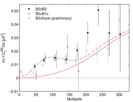
Although the BICEP-2 collaboration’s analysis took as a prior in its simulated data, we wish to ask whether a suppression of power in the BB angular power spectrum at large angular scales relative to smaller scales might be seen in the data, in particular in the B2 x Keck cross correlation function at long wavelengths (which is less sensitive to systematic noise222Which we note can only boost the auto-correlation function.) and in the B2 x B2 correlation function, although the latter is more susceptible to contamination from foregrounds (see Fig. 1). Whether this suppression is statistically significant remains to be seen. If it is, it could be interpreted as indicative of a positive tilt of the primordial tensor spectrum at the largest angular scales. If this does turn out to be the case, then this result would be very hard to interpret in the context of the standard inflationary paradigm of early universe cosmology (see also contaldi for an analysis of the additional tension between measuring a large with the small scalar power spectrum).
Assuming that space-time is described by General Relativity and that matter obeys the “weak energy condition”, inflation generically predicts a red spectrum of gravitational waves, i.e. . This arises from the fact that the amplitude of the gravitational waves on a scale is set by the amplitude of the Hubble expansion rate at the time when that scale exits the Hubble radius, and that during inflation . For single field slow roll models this relation is precisely
| (1) |
with . A related challenge for standard inflationary cosmology in light of the BICEP-2 data is that the tensor-to-scalar ratio implies a large field excursion over the duration in which the observed modes in the CMB were produced Lyth :
| (2) |
Constructing a model that safely accomplishes this is challenging to say the least from the perspective of effective field theory, as field excursions comparable to the cut-off of the theory typically generate large anomalous dimensions for operators that were initially suppressed (by appropriate powers of the cutoff), potentially spoiling the requisite conditions for inflation to occur as it progresses333The so called sensitivity of large field models to ‘Planck slop’ BCQ .. However, this is not to say that this might not be accomplished in the context of some fundamental theory construction– see SW for an interesting claim (and JC for a counter-claim)– within the context of string theory, large field excursions certainly appear to be problematic swampland .
In this note we wish to remind cosmologists of a mechanism to generate the primordial perturbations from the thermodynamics of closed strings in a quasi-static background, which–
-
•
Naturally generates a large tensor to scalar ratio;
-
•
Predicts a blue tilt to the tensor spectrum,
-
•
with a complimentary red tilt to the scalar spectrum, both of which relate to .
This construction relies upon a background that consists of a quasi-static initial state in the Einstein frame, whose specific realization can be addressed in the context of particular string constructions (see Florakis ; KPT1 for some recent attempts), but whose existence we will take for granted in the following as far as the study of fluctuations is concerned, just as one typically does in the context of inflationary cosmology444Requiring that inflation exists in the context of a consistent quantum theory requires considerable tuning at the level of the low energy effective description ETA (its so-called UV sensitivity).. In fact, this is the very premise of the effective theory of the adiabatic mode Senatore – the so called effective theory of inflation. In what follows, we will first address plausible constructions that could give rise to the requisite background as motivation for the subsequent section– the main focus of this note– where we argue that the thermodynamics of closed strings in the early universe can naturally generate a large, blue titled tensor mode background.
Our goal is to provide observations with a novel, predictive, and falsifiable model which can inform the formulation of priors when analyzing the data in a manner that is easily contrasted against the predictions of inflationary cosmology. Whether there are hints for a blue tensor tilt in the data is to be viewed as secondary to the goal of providing a ‘straw-model’ with which to contrast the predictions of inflation against, the scientific utility of which needing no further elaboration.
II Closed string thermodynamics and a quasi static initial universe
The geometry of string theory is a very rich and complex subject. There exist very distinct geometries, sometimes with very distinct topologies that are indistinguishable from each other as far as physical processes involving strings are concerned. Known as ‘dualities’ GPR , the connections between these geometries is one of the most striking features of string theory that persists at low energies, a pervasive manifestation of which is the T-duality symmetry that relates strings in a very large universe (relative to the string scale) to strings in a very small universe. In the absence of any background fluxes, in the context of Heterotic string theory for example, this implies the duality
| (3) |
Where is the (target space) metric of spacetime. The implications of this duality on early universe cosmology has been studied extensively in various constructions PBB ; TV . The particular context we are concerned with, “string gas cosmology”, is a paradigm of early universe cosmology initially proposed in BV to explain why only three of the nine spatial dimensions of string theory can be macroscopic. Within a particular realization of this framework, given certain assumptions, one can naturally generate a large tensor background with a spectrum that is blue tilted BNPV , with a red tilted scalar spectrum NBV 555As has been remarked since this model was proposed SGCrevs , a detection of a blue spectrum of tensor modes can be viewed as a prediction for cosmological observations, first made in the context of string theory, that would falsify the inflationary paradigm if obserevd..
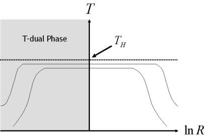
The cosmological model we consider NBV ; BNPV is based on the thermodynamics of closed heterotic strings. Due to the existence of an exponential tower of oscillatory string modes, there is a maximal temperature which a thermal gas of strings can attain Hagedorn . The existence of winding modes in addition to the center-of-mass momentum modes is the representation of the T-duality (3) on the matter content of the universe, wherein physics on a torus of radius is equivalent to that on a torus of radius , where is the string length. This duality leads to the temperature/radius curve for a weakly coupled gas of strings indicated in Figure 2 (where the vertical axis is the temperature, and the horizontal axis the radius in string units on a logarithmic scale). It thus seems reasonable to conjecture that the cosmological singularity might be dynamically resolved by the energetics of the so called Hagedorn phase666As has been explicitly demonstrated in the context of type II strings in KPT1 ; KPT2 ..
The model of NBV ; BNPV is based on the premise that the universe starts in the quasi-static Hagedorn phase when the temperature is only very slightly lower than the Hagedorn temperature 777As explained in BV , the temperature difference depends inversely on the entropy. The decay of string winding modes will eventually enable three spatial dimensions to become large, while the others are forever confined by string winding modes BV 888The role played by T-duality in ensuring moduli stabilization was discussed in detail in moduli .. The decay of the string winding modes leads to a smooth transition to the radiation-dominated phase of Standard Cosmology. The transition time between the quasi-static Hagedorn phase with constant scale factor and the radiation phase with is denoted by , since it plays a role similar to the reheating time in inflationary cosmology.
In Figure 3 we show the evolution of various scales in string gas cosmology. In this sketch, the vertical axis is time, the horizontal axis represents physical distance. The two light red curves which are vertical in the Hagedorn phase indicate the physical wavelengths of two different fluctuation modes. The solid blue curve which grows linearly in the radiation phase and is at infinity early in the Hagedorn phase is the Hubble radius , the inverse expansion rate (where the dot indicates the derivative with respect to time ). The Hubble radius separates scales on which fluctuations oscillate (sub-Hubble modes) from those where the oscillations are frozen out and the amplitude of the modes is squeezed (see MFB for discussions of how cosmological perturbations evolve), namely the super-Hubble modes.
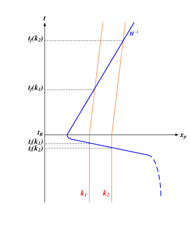
The first point to remark is that the horizon is much larger than the Hubble radius (in fact infinite if time extends to ). Hence, string gas cosmology addresses the horizon problem of standard cosmology in a complimentary way to inflation. Secondly, it is clear that cosmological fluctuations begin on sub-Hubble scales and evolve after for a long time at super-Hubble lengths. The sub-Hubble origin of the scales makes it possible to have a causal generation mechanism of fluctuations, the super-Hubble period of evolution will lead to acoustic oscillations at late times in both the angular power spectrum of CMB anisotropies and in the matter power spectrum SZ .
Having set the scene for the background, we now turn to reviewing why this string cosmological background can lead to a spectrum of cosmological perturbations with a red tilt and gravitational waves with a blue tilt, generated by the thermodynamics of strings.
III Tensor Modes from an early Hagedorn phase
Since in the initial Hagedorn phase of string cosmology matter is a thermal gas of strings, the initial conditions for scalar and tensor metric fluctuations are thermal rather than vacuum and the energy-momentum tensor correlation functions are determined by closed string thermodynamics rather than by open or point particle thermodynamics Ali .
The calculation of the spectrum of scalar NBV and tensor BNPV fluctuations in string gas cosmology proceeds in three steps. In the first, the matter correlation functions are evaluated using the results of the closed string thermal partition function given in Deo . The second step is to use the Einstein constraint equations, presuming our quasi-static background to be a given in the Einstein frame999From more we know this is a non-trivial assumption. However, see KPT1 for suggestions as to how one could accomplish this in the context of type II superstrings., to determine the cosmological fluctuations and gravitational waves from the matter correlation functions mode by mode when the modes exit the Hubble radius at the times . The third step is to evolve the gravitational fluctuations until the present time using the usual theory of cosmological fluctuations.
The metric including cosmological fluctuations and gravitational waves can be written in the form MFB
| (4) |
where is conformal time related to physical time via . The scalar metric fluctuations are determined via the energy density perturbations via
| (5) |
where the pointed brackets indicate thermal expectation values, is the energy-momentum tensor, and is Newton’s gravitational constant. The gravitational waves are given by the off-diagonal (i.e. ) pressure fluctuations:
| (6) |
To determine the energy density fluctuations, we use the fact that in thermal equilibrium the position space perturbations are given by the specific heat capacity at fixed volume
| (7) |
For a thermal gas of heterotic strings is given by
| (8) |
and hence the power spectrum of , defined by
| (9) |
is determined to be NBV
| (10) |
where is the temperature at the time when mode exits the Hubble radius.
As inferred from Figures 2 & 3, the temperature decreases as increases, since large modes exit the Hubble radius later. Since is close to the Hagedorn temperature, it is the denominator of the right hand side of (10) which dominates the final amplitude. Hence, the spectrum of scalar metric fluctuations has a red tilt (larger amplitude at larger wavelengths). Neglecting running, the tilt can be computed as (defining )
| (11) |
which is negative since , and arbitrarily small in the limit of a sudden transition (in which case ). The power spectrum of the tensor modes, which is produced by fluctuations of the wound strings around a compact space, is given by (6) the correlation function () , namely the mean square fluctuation of () in a region of radius
| (12) |
The correlation function on the right hand side of the above equation follows from the thermal closed string partition function and was computed in Ali ; BNPV2 (see also new for a more general treatment), with the result that for temperatures close to the Hagedorn value
| (13) |
The key factor now appears in the numerator and hence leads to a blue spectrum. Neglecting running (and thus the logarithmic factor as well), the tilt can be computed as
| (14) |
where we see the complimentarity between the tilt of the scalar and tensor spectra. The fact that we obtain a blue spectrum of gravitational waves is readily understood. The spectrum of gravitational waves is determined by the anisotropic pressure perturbations. Since deeper in the Hagedorn phase, i.e. at higher , the pressure is smaller, the anisotropic pressure fluctuations should be smaller, as well. Hence, the amplitude of the gravitational wave spectrum will increase towards the ultraviolet, corresponding to a blue spectrum. Furthermore, we can also compute the tensor to scalar ratio as
| (15) |
Requiring COBE normalization for the power spectrum for the comoving curvature perturbation NBV , in addition to requiring a tensor to scalar ratio of BICEP fixes the string length to be given by , and that the modes we observe exited when the temperature of the universe was . The latter implying that the tensor tilt is essentially equal and opposite to the scalar tilt
| (16) |
the precise value of which depends on the manner in which the background exited the Hagedorn phase.
IV Discussion
In generating the primordial perturbations from the thermodynamics of closed strings, one can isolate the background dependence to one free parameter, the ratio of string length and Planck length, and a function which is close to the Hagedorn temperature and is a decreasing function of . The precise dependence depends of encodes the details of the transition between the Hagedorn phase and the radiation phase, and will determine the relative tilts of the spectra (11) and (14), which are to first approximation, equal and opposite (14). With these inputs we can also compute the amplitudes of the scalar and tensor spectra at any pivot scale, which is unique for only three spatial large compact dimensions Ali . As emphasized in BNPV , the key result is that the tensor spectrum has a blue tilt, whereas the scalar fluctuations retain a red tilt. This feature distinguishes the string thermodynamic generation of the primordial perturbations from standard inflationary realizations.
Acknowledgements.
We wish to thank Matt Dobbs, Gil Holder and Cumrun Vafa for valuable discussions and correspondence. SP is supported by a Marie Curie Intra-European Fellowship of the European Community’s 7’th Framework Program under contract number PIEF-GA-2011-302817. RB is supported by an NSERC Discovery Grant, and by funds from the Canada Research Chair program.References
- (1) [BICEP2 Collaboration], BICEP2 I: Detection Of B-mode Polarization at Degree Angular Scales”, arXiv:1403.3985.
- (2) R. J. Danos, R. H. Brandenberger and G. Holder, “A Signature of Cosmic Strings Wakes in the CMB Polarization,” Phys. Rev. D 82, 023513 (2010) [arXiv:1003.0905 [astro-ph.CO]].
- (3) D. Hanson et al. [SPTpol Collaboration], “Detection of B-mode Polarization in the Cosmic Microwave Background with Data from the South Pole Telescope,” Phys. Rev. Lett. 111, 141301 (2013) [arXiv:1307.5830 [astro-ph.CO]].
- (4) [The POLARBEAR Collaboration], “A Measurement of the Cosmic Microwave Background B-Mode Polarization Power Spectrum at Sub-Degree Scales with POLARBEAR,” arXiv:1403.2369 [astro-ph.CO].
- (5) C. R. Contaldi, M. Peloso and L. Sorbo, “Suppressing the impact of a high tensor-to-scalar ratio on the temperature anisotropies,” arXiv:1403.4596 [astro-ph.CO].
- (6) D. H. Lyth, “What would we learn by detecting a gravitational wave signal in the cosmic microwave background anisotropy?,” Phys. Rev. Lett. 78, 1861 (1997) [hep-ph/9606387].
- (7) C. P. Burgess, M. Cicoli and F. Quevedo, “String Inflation After Planck 2013,” JCAP 1311, 003 (2013) [arXiv:1306.3512, arXiv:1306.3512 [hep-th]].
- (8) E. Silverstein and A. Westphal, “Monodromy in the CMB: Gravity Waves and String Inflation,” Phys. Rev. D 78, 106003 (2008) [arXiv:0803.3085 [hep-th]].
- (9) J. P. Conlon, “Brane-Antibrane Backreaction in Axion Monodromy Inflation,” JCAP 1201, 033 (2012) [arXiv:1110.6454 [hep-th]].
- (10) C. Vafa, “The String landscape and the swampland,” hep-th/0509212; H. Ooguri and C. Vafa, Nucl. Phys. B 766, 21 (2007) [hep-th/0605264].
- (11) I. Florakis, C. Kounnas, H. Partouche and N. Toumbas, “Non-singular string cosmology in a 2d Hybrid model,” Nucl. Phys. B 844, 89 (2011) [arXiv:1008.5129 [hep-th]].
- (12) C. Kounnas, H. Partouche and N. Toumbas, “S-brane to thermal non-singular string cosmology,” Class. Quant. Grav. 29, 095014 (2012) [arXiv:1111.5816 [hep-th]].
- (13) C. P. Burgess and L. McAllister, “Challenges for String Cosmology,” Class. Quant. Grav. 28, 204002 (2011) [arXiv:1108.2660 [hep-th]]; S. Hardeman, J. M. Oberreuter, G. A. Palma, K. Schalm and T. van der Aalst, “The everpresent eta-problem: knowledge of all hidden sectors required,” JHEP 1104, 009 (2011) [arXiv:1012.5966 [hep-ph]].
- (14) C. Cheung, P. Creminelli, A. L. Fitzpatrick, J. Kaplan and L. Senatore, “The Effective Field Theory of Inflation,” JHEP 0803, 014 (2008) [arXiv:0709.0293 [hep-th]].
- (15) A. Giveon, M. Porrati and E. Rabinovici, “Target space duality in string theory,” Phys. Rept. 244, 77 (1994) [hep-th/9401139].
- (16) M. Gasperini and G. Veneziano, “Pre - big bang in string cosmology,” Astropart. Phys. 1, 317 (1993) [hep-th/9211021]; M. Gasperini and G. Veneziano, “The Pre - big bang scenario in string cosmology,” Phys. Rept. 373, 1 (2003) [hep-th/0207130].
- (17) A. A. Tseytlin and C. Vafa, “Elements of string cosmology,” Nucl. Phys. B 372, 443 (1992) [hep-th/9109048].
- (18) R. H. Brandenberger and C. Vafa, “Superstrings In The Early Universe,” Nucl. Phys. B 316, 391 (1989).
- (19) R. H. Brandenberger, A. Nayeri, S. P. Patil and C. Vafa, “Tensor Modes from a Primordial Hagedorn Phase of String Cosmology,” Phys. Rev. Lett. 98, 231302 (2007) [hep-th/0604126].
- (20) A. Nayeri, R. H. Brandenberger and C. Vafa, “Producing a scale-invariant spectrum of perturbations in a Hagedorn phase of string cosmology,” Phys. Rev. Lett. 97, 021302 (2006) [arXiv:hep-th/0511140].
-
(21)
R. H. Brandenberger, A. Nayeri, S. P. Patil and C. Vafa,
“String gas cosmology and structure formation,”
Int. J. Mod. Phys. A 22, 3621 (2007)
[hep-th/0608121];
R. H. Brandenberger, “String Gas Cosmology,” arXiv:0808.0746 [hep-th]. - (22) R. Hagedorn, “Statistical Thermodynamics Of Strong Interactions At High-Energies,” Nuovo Cim. Suppl. 3, 147 (1965).
- (23) C. Kounnas, H. Partouche and N. Toumbas, “Thermal duality and non-singular cosmology in d-dimensional superstrings,” Nucl. Phys. B 855, 280 (2012) [arXiv:1106.0946 [hep-th]]; R. H. Brandenberger, C. Kounnas, H. éPartouche, S. P. Patil and N. Toumbas, “Cosmological Perturbations Across an S-brane,” JCAP 1403, 015 (2014) [arXiv:1312.2524 [hep-th]].
- (24) S. P. Patil and R. Brandenberger, “Radion stabilization by stringy effects in general relativity and dilaton gravity,” Phys. Rev. D 71, 103522 (2005) [arXiv:hep-th/0401037]; S. Watson, “Moduli stabilization with the string Higgs effect,” Phys. Rev. D 70, 066005 (2004) [arXiv:hep-th/0404177]; L. Kofman, A. Linde, X. Liu, A. Maloney, L. McAllister and E. Silverstein, “Beauty is attractive: Moduli trapping at enhanced symmetry points,” JHEP 0405, 030 (2004) [arXiv:hep-th/0403001]; S. P. Patil and R. H. Brandenberger, “The cosmology of massless string modes,” JCAP 0601, 005 (2006) [arXiv:hep-th/0502069]; R. Brandenberger, Y. K. Cheung and S. Watson, “Moduli stabilization with string gases and fluxes,” JHEP 0605, 025 (2006) [arXiv:hep-th/0501032]; R. J. Danos, A. R. Frey and R. H. Brandenberger, “Stabilizing moduli with thermal matter and nonperturbative effects,” Phys. Rev. D 77, 126009 (2008) [arXiv:0802.1557 [hep-th]]; S. Mishra, W. Xue, R. Brandenberger and U. Yajnik, “Supersymmetry Breaking and Dilaton Stabilization in String Gas Cosmology,” JCAP 1209, 015 (2012) [arXiv:1103.1389 [hep-th]].
-
(25)
V. F. Mukhanov, H. A. Feldman and R. H. Brandenberger,
“Theory of cosmological perturbations. Part 1. Classical perturbations. Part
2. Quantum theory of perturbations. Part 3. Extensions,”
Phys. Rept. 215, 203 (1992);
R. H. Brandenberger, “Lectures on the theory of cosmological perturbations,” Lect. Notes Phys. 646, 127 (2004) [arXiv:hep-th/0306071]. -
(26)
R. A. Sunyaev, Y. .B. Zeldovich,
“Small scale fluctuations of relic radiation,”
Astrophys. Space Sci. 7, 3-19 (1970);
P. J. E. Peebles, J. T. Yu, “Primeval adiabatic perturbation in an expanding universe,” Astrophys. J. 162, 815-836 (1970). - (27) N. Deo, S. Jain, O. Narayan and C. I. Tan, “The Effect of topology on the thermodynamic limit for a string gas,” Phys. Rev. D 45, 3641 (1992).
- (28) R. H. Brandenberger, S. Kanno, J. Soda, D. A. Easson, J. Khoury, P. Martineau, A. Nayeri and S. P. Patil, “More on the spectrum of perturbations in string gas cosmology,” JCAP 0611, 009 (2006) [hep-th/0608186].
- (29) A. Nayeri, “Inflation free, stringy generation of scale-invariant cosmological fluctuations in D = 3 + 1 dimensions,” arXiv:hep-th/0607073.
- (30) R. H. Brandenberger, A. Nayeri, S. P. Patil and C. Vafa, “String gas cosmology and structure formation,” Int. J. Mod. Phys. A 22, 3621 (2007) [hep-th/0608121].
- (31) T. Biswas, R. Brandenberger, T. Koivisto and A. Mazumdar, “Cosmological perturbations from statistical thermal fluctuations,” Phys. Rev. D 88, no. 2, 023517 (2013) [arXiv:1302.6463 [astro-ph.CO]].