Bicep2 II: Experiment and Three-Year Data Set
Abstract
We report on the design and performance of the Bicep2 instrument and on its three-year data set. Bicep2 was designed to measure the polarization of the cosmic microwave background (CMB) on angular scales of 1 to 5 degrees (–), near the expected peak of the -mode polarization signature of primordial gravitational waves from cosmic inflation. Measuring -modes requires dramatic improvements in sensitivity combined with exquisite control of systematics. The Bicep2 telescope observed from the South Pole with a 26 cm aperture and cold, on-axis, refractive optics. Bicep2 also adopted a new detector design in which beam-defining slot antenna arrays couple to transition-edge sensor (TES) bolometers, all fabricated on a common substrate. The antenna-coupled TES detectors supported scalable fabrication and multiplexed readout that allowed Bicep2 to achieve a high detector count of 500 bolometers at 150 GHz, giving unprecedented sensitivity to -modes at degree angular scales. After optimization of detector and readout parameters, Bicep2 achieved an instrument noise-equivalent temperature of . The full data set reached Stokes and map depths of 87.2 nK in square-degree pixels () over an effective area of 384 square degrees within a 1000 square degree field. These are the deepest CMB polarization maps at degree angular scales to date. The power spectrum analysis presented in a companion paper has resulted in a significant detection of -mode polarization at degree scales.
Subject headings:
cosmic background radiation — cosmology: observations — gravitational waves — inflation — instrumentation: polarimeters — telescopes3.1. Observing site
The South Pole is an excellent site for millimeter-wave observation from the ground, with a record of successful polarimetry experiments including Dasi, Bicep1, QUaD and the South Pole Telescope. Situated on the Antarctic Plateau, it has exceptionally low precipitable water vapor (chamberlin1997), reducing atmospheric noise due to the absorption and emission of water near the observing band. The South Pole site also has very stable weather, especially during the dark winter months, so that the majority of the data are taken under clear-sky conditions of very low atmospheric noise and low loading (stark02). The consistently low atmospheric loading is crucially important because the sensitivity of the experiment is limited by photon noise, so that low atmospheric emission is a key to high CMB mapping speed.
Finally, the Amundsen-Scott South Pole Station has hosted scientific research continuously since 1958. The station offers well-developed facilities with year-round staff and an established transportation infrastructure. Bicep1 and Bicep2 were housed in the Dark Sector Laboratory (DSL), which was built to support radio and millimeter-wave observatories in an area from the main station buildings and isolated from possible sources of electromagnetic interference.
3.2. Telescope mount and drive
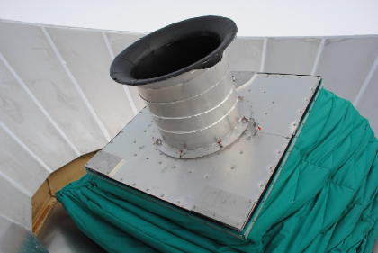 |
The telescope sat in a three-axis mount (Fig. LABEL:fig:mount) supported on a steel and wood platform attached to the structural beams of the DSL building. The mount was originally built for Bicep1 by Vertex-RSI111Now General Dynamics Satcom Technologies, Newton, NC 28658, http://www.gdsatcom.com/vertexrsi.php along with a second, identical mount that has remained in North America for pre-deployment testing. The mount attached to a flexible environmental shield or “boot” (Fig. 2) attached to the roof of the building, so that the cryostat, electronics, and drive hardware were kept inside a climate-controlled, room temperature environment.
The mount moved in azimuth and elevation (which closely approximate right ascension and declination when observing from the South Pole). Its third axis was a rotation about the boresight of the telescope, also known as the “deck angle”. When installed in DSL its range of motion was – in elevation and in azimuth. It was capable of scanning at speeds of up to in azimuth. The major modification for Bicep2 was the replacement of a slip ring with a cylindrical drum through which the readout and control cables were fed. This accommodates the much larger bundle of cables needed for the Bicep2 housekeeping system (§8.4) while retaining a range of rotation of 380∘ in boresight angle. Our selection of boresight angles for observing therefore remained unrestricted.
4. Optics
The Bicep2 telescope (Fig. 4) was an on-axis refractor similar to Bicep1 (takahashi10), with an aperture of and beams of width given by the Gaussian radius . The relatively simple optical design (Fig. 4) and small aperture allowed Bicep2 to target the predicted degree-scale peak of the inflationary -mode signal while avoiding reflective components that add expense and complexity and can have significant instrumental polarization. The telescope was efficient to assemble and transport. This design also allowed all optics to be cooled to 4 K for low optical loading, and the beams to be measured in the far field () using controlled optical sources on the ground. The low loading and the ability to extensively characterize the beams have been important for achieving high sensitivity and control of beam systematics, respectively.
4.1. Lenses and optical simulation
The telescope was designed to produce very well-matched beams for two orthogonal linear polarizations coincident on the sky. The two lenses were made of high density polyethylene and were roughly in diameter. The lens shapes and placement, along with other components of the optical design, were guided by simulation of the beam properties using the Zemax optical design software222ZEMAX Development Corporation, Redmond, WA 98053, http://www.zemax.com/. We chose to place the first Airy null at the aperture stop for low internal loading. This approximately satisfies the criterion of griffin02 for a wavelength . The other constraints on the optimization process were to minimize aberration and maintain telecentricity. The resulting configuration has an effective focal length of and a lens separation of . Further details of the simulation and optimization may be found in aikin10 and aikinthesis.
Simulation of the selected design predicts a nearly ideal Gaussian beam with width (FWHM=) and cross-polar response below . The simulated beams for the two detectors in each pair are the same to below in ellipticity, in beam width, and in pointing (as a fraction of beam width). These ideal parameters can be compared to the performance of the instrument as built. The polarization response was measured in far-field and near-field calibration tests (§11.4), which found no intrinsic cross-polar response detectable above the level of known instrumental crosstalk (). The achieved beams have also been extensively measured in the far field (§11.2), allowing our analysis to fully account for any departures from the ideal beams predicted by the optics simulation.
4.2. Vacuum window
The vacuum window was 32 cm in diameter and 12 cm thick, made of four layers of Propozote PPA30 foam333Zotefoams Inc., Walton, KY 41094, http://zotefoams.com/ joined into a single piece by heat lamination. The PPA30 material is a closed-cell, nitrogen-filled polypropylene foam with low scattering and high microwave transmission (tophat; runyan03). The window was sealed to its aluminum housing with Stycast 1266 epoxy.
4.3. Optical loading reduction
| Element | [K] | Emissivity | Loading [pW] | [K] |
|---|---|---|---|---|
| CMB | 3 | 1.00 | 0.12 | |
| Atmosphere | 230 | 0.03 | 2.0 | |
| Upper Forebaffle | 230 | 1.00 | 0.65 | |
| Window | 230 | 0.02 | 1.0 | |
| IR Blocker 1 | 100 | 0.02 | 0.45 | |
| IR Blocker 2 | 40 | 0.02 | 0.18 | |
| IR Blocker 3 | 40 | 0.02 | 0.18 | |
| IR Blocker 4 | 6 | 0.02 | 0.01 | |
| Lenses | 6 | 0.10 | 0.07 | |
| Total | 4.7 | 22 |
Optical loading contributes to photon noise, which sets the ultimate sensitivity of the experiment. We have therefore taken care to minimize internal loading by ensuring that all microwave power reaching the detectors comes only from the sky or cold surfaces. This was accomplished by intercepting stray radiation at a cold aperture stop and blackening reflective surfaces. The aperture stop, which defines the beam waist, was an annular ring of thick Eccosorb AN-74444Emerson & Cuming Microwave Products, Randolph, MA 02368. http://eccosorb.com/ with inner diameter . It was placed on the lower surface of the objective lens at as shown in Fig. 4. Given the optical design parameters described above, we calculate that the aperture stop absorbed 20% of total optical throughput. The sides of the tube supporting the optics and the magnetic shield (§5.3) were blackened using carbon-loaded Stycast 2850 FT epoxy applied to a surface of roughened Eccosorb HR10. This black surface has very low reflectivity, and is especially effective in minimizing specular reflection. This textured black surface cycles cryogenically with minimal particulate shedding, and has very low reflectivity even at low angles of incidence.
Following an approach developed in Bicep1, we placed two polytetrafluoroethylene (PTFE) filters in front of the objective lens to reduce thermal loading by absorbing infrared radiation. These were heat sunk to and . We placed a thick nylon filter in front of the objective lens, heat sunk to . In addition, we placed a thick nylon filter in front of the eyepiece lens, heat sunk to . We finally added a metal mesh low-pass edge filter (ade06) with a cutoff at () to reflect any coupling to submillimeter radiation not absorbed in the plastic filters. This filter was placed directly below the nylon filter and was also cooled to 4 K.
We have modeled the expected loading for each optical component and the atmosphere as shown in Table 1. In the table, the emission temperature and estimated emissivity are given for each optical element. These are combined with measured optical efficiencies for Bicep2 (§10.2) The total loading is also expressed in units of Rayleigh-Jeans temperature . Although the absorptive upper forebaffle had an emissivity of 1, the aperture stop and blackening of the optics tube limited sidelobes sufficiently that the forebaffle only intercepted 1% of the beam and contributed an acceptably low loading power. The 0.65 pW forebaffle loading in Tab. 1 is a measured value from tests with and without the forebaffle installed, as described in Section 11.3. The loading from internal components have been calculated in the model with a total internal loading of 1.89 pW. This is consistent with laboratory test measurements (§10.4) that give an upper limit of 2.2 pW.
4.4. Antireflection coating
Both lenses and the IR blocking filters have been coated with an antireflection (AR) layer of porous PTFE (Mupor555Porex Corporation, Fairburn, GA 30213, http://www.porex.com/) optimized for . The PTFE thickness and density were chosen to minimize reflection given the index of refraction of each optical element. The AR layers were heat-bonded using a thin low-density polyethylene (LDPE) film as a bonding layer. In order to ensure uniform adhesion, the AR layer and LDPE film were pressed against the surface by enclosing each optical element in a vacuum bag during heat-bonding.
The metal mesh low-pass edge filter was separately coated with an antireflection layer during its fabrication at Cardiff University.
4.5. Membrane
In front of the window was a 0.5 mil () transparent membrane held tautly in place by two aluminum rings. The membrane protected the window from snow and created an enclosed space below, which was slightly pressurized with dry nitrogen gas to prevent condensation on the Propozote foam. Room-temperature air flowed through holes in the ring onto the top of the membrane so that any outside snowfall sublimated away.
The initially deployed membrane was thick biaxially oriented polyethylene terephthalate (Mylar), which is expected to have reflectivity of only 0.2% at 150 GHz. During maintenance at the end of 2010 this was replaced with a sheet of the same material and thickness, but held very taut within the aluminum rings. Vibrations of the new membrane caused intermittent common-mode noise, strongly correlated across detectors. We have verified that this noise does not significantly contaminate the pair-differenced polarization maps, but as a precaution we remove the most affected data using a cut on noise correlation (§13.7). The membrane was replaced again on 2011 April 27 with less taut, thick biaxially oriented polypropylene (BOPP), while the pressure of the nitrogen gas purge was adjusted to minimize vibration. After these changes the membrane noise signal was not seen in the remainder of the 2011–12 data set.
5. Telescope insert
The entire telescope at and colder formed a removable insert that was installed into the cryostat (Fig. 5). The upper part of this insert was the optics tube, which contained the cold lenses and the infrared-blocking filters. The bottom section of the insert, called the camera tube, held the detector array, cold electronics, and 3He/3He/4He sorption refrigerator. The bottom plate of the insert was directly connected to the helium bath. This plate provided sufficient cooling power at to cool the optics inside the telescope tube and to allow the refrigerator to condense liquid 4He.
5.1. Carbon fiber truss structure
The focal plane sat near the break between the camera tube and the optics tube. It required a compact, rigid support structure with low thermal conductance to the walls of the aluminum tube at 4 K. This support was provided by sets of concentric carbon-fiber truss structures connecting the thermal stages at , , , and . The trusses between the plate and the focal plane are shown schematically in Fig. 5 and can also be seen in the left-hand panel of Fig. 6. The carbon fiber has excellent mechanical properties and has a very low ratio of thermal conductivity to strength at temperatures below a few kelvin (runyan08).
5.2. RF shielding
The detectors and cold SQUID readout electronics were enclosed in a radio frequency (RF) shield depicted in Fig. 5. The RF shield began on the top of the focal plane, just above the detector arrays. A square clamp held an aluminized Mylar shroud (Fig. 5) that extended from around the detectors down to a circular clamp to the 350 mK niobium (Nb) plate. A second Mylar sheet was used to create a conductive path that surrounds the stages at different temperatures without thermally linking them. This sheet went up from the ring to a ring, and then down to the ring. This ring connected to the aluminum walls of the optics and camera tubes and the base plate of the camera tube. Filter connectors at the base plate protected the cold electronics from RF interference picked up in wiring outside the cryostat.
|
5.3. Magnetic shielding
The SQUIDs, TESs, and other superconducting components are sensitive to ambient magnetic fields, including those of the Earth and of nearby electrical equipment such as the telescope drive motors. We attenuated the field in the vicinity of all sensitive elements by surrounding them with passive magnetic shielding. The final shielding configuration was chosen after simulation using COMSOL Multiphysics software666COMSOL, Inc., Burlington, MA 01803, http://www.comsol.com/ and experimentation with various options for each susceptible component. This process led to the selection of superconducting and high-permeability shielding materials according to their measured effectiveness in each location.
The focal plane assembly was surrounded to the greatest extent possible by a superconducting shield shown in Fig. 5. This shield was composed of the Nb plate at the 350 mK stage beneath the focal plane, a Nb plate immediately in front of the focal plane, and a cylindrical Nb shield that extends from the 350 mK plate upward. The Nb backshort immediately behind the detector tiles provided additional shielding.
A cylinder of thick Cryoperm 10 alloy777Amuneal Manufacturing Corp., Philadelphia, PA 19124, http://amuneal.com/ was wrapped around the entire optics tube and held at . This high-permeability shield drew field lines into itself so that they would not be trapped in the superconducting Nb shield around the focal plane.
We placed sheets of Metglas 2714A888Metglas, Inc., Conway, SC 29526, http://www.metglas.com/products/magnetic_materials/ behind the printed circuit board that housed the first and second-stage SQUIDs (Fig. 5.3). In laboratory comparisons this was found to give greater attenuation of applied fields than Nb foil in this location.
Early tests showed that the instrument’s magnetic sensitivity was dominated by the SQUID series arrays (SSAs), which were located outside the focal plane assembly, on the side of the refrigerator (Fig. 5). The SQUID arrays were already enclosed in superconducting Nb shielding within the SSA modules, and this shielding was greatly improved by wrapping several layers of Metglas 2714A around the SSA modules. After this improvement the level of magnetic sensitivity from the SSAs was much lower than that at other stages.
We characterized the remaining level of magnetic sensitivity in laboratory tests by placing a Helmholtz coil in three orientations around the cryostat, and in situ by performing ordinary CMB observing schedules with the TES detectors deliberately inactive. We found that the shielding achieved an overall suppression factor of , leaving a residual signal from the Earth’s magnetic field. This had a median size corresponding to , or up to in the most sensitive channels. The sensitivity was dominated by the first-stage SQUIDs, which were especially sensitive in the MUX07a generation of hardware (stiehl11). The remaining signal has a simple sinusoidal form in azimuth and is ground-fixed, so that it can be removed very effectively in analysis by low-order polynomial subtraction (§13.5) and ground-fixed signal subtraction (§13.6).
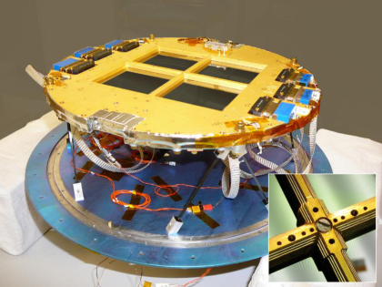
6. Focal Plane
The focal plane unit (FPU) was constructed from several layers of different materials selected to provide the stable temperature, mechanical alignment, and magnetic shielding required to operate the camera. The detector tiles must be held firmly in place while allowing for differential thermal contraction and providing sufficient thermal conduction to the refrigerator. The temperature of the focal plane must be kept very stable. Sensitive components must be further shielded from stray magnetic fields. Finally, the optical backshort must be precisely aligned at a quarter wavelength behind the detector tiles. We have achieved these goals using the focal plane components described below.
6.1. Copper plate
The focal plane was assembled around a gold-plated, oxygen-free high thermal conductivity copper (OFHC Cu) detector plate. The detector tiles and most other focal plane components were mounted to its lower face. The Cu plate with detector tiles and multiplexing components mounted can be seen in the right-hand panel of Fig. 6, and an exploded view of all layers in the assembly is shown in Fig. 5.3. In the plate were four square windows that allowed radiation to reach the detectors. To suppress electromagnetic coupling between the detector plate and the antennas of pixels near the tile edges, we cut quarter-wavelength-deep corrugations (Fig. 6 left, inset) into the edges of the windows (orlando10).
6.2. Niobium backshort
A superconducting niobium (Nb) plate sat below the Cu at a separation of and served as an optical backshort. It was held at the correct distance by precision-ground Macor999Corning Incorporated, Corning, NY 14831, http://www.corning.com/specialtymaterials/macor/ washers, whose thermal contraction is negligible when cooled to millikelvin temperatures. The Nb backshort was supported at its perimeter by a carbon-fiber truss and cooled at its center through a Cu foil strap (§8.3). This contact point ensured that the Nb backshort transitions into a superconducting state from the center outwards so that it would not trap flux as is possible with type-II superconductors.
6.3. Printed circuit board
An FR-4 printed circuit board (PCB) carried superconducting Al electrical traces and served as a base for wire-bonding the tiles and the SQUID chips. Between the Cu plate and the PCB we placed sheets of Metglas 2714A to create a low-field environment around the SQUID chips. The planar geometry between the Cu and Nb plates was especially effective in lowering the normal field component to which the SQUID chips are most sensitive. The SQUIDs sat on alumina carriers on the PCB, giving sufficient separation from the Metglas sheet to prevent magnetic coupling that could cause increased readout noise.
6.4. Assembly
Each detector tile was stacked with a high-conductivity -cut crystal quartz anti-reflection (AR) wafer. We attached the detector tiles and AR wafers to the Cu plate in a way that provided precision alignment, allowed for differential thermal contraction, and ensured sufficient heat-sinking. First precision-drilled holes and slots were made in the detector tiles and AR wafers. These registered to pins that were press-fit in the Cu adjacent to each window. The detector tile and AR wafer stacks were clamped to the plate with machined tile clamps that allow slipping under thermal contraction. The weak clamping force was insufficient to effectively heat-sink the tiles, so we further connected a gold “picture frame” around the tile edges with gold wire bonds that made direct contact with the gold-plated Cu frame. The thermal conductivity (limited by the Kapitza resistance between the silicon substrate and the gold) was large enough to prevent tile heating under thermal loading.
Additional wire bonds were used to electrically connect mounted components to traces in the PCB. The detector tiles had Nb pads on their back edges to be connected to the PCB traces with superconducting Al wire bonds. The SQUID chips (§9.1) were similarly wire-bonded to the PCB, as were NTD thermometers and heaters mounted directly on the detector tiles.
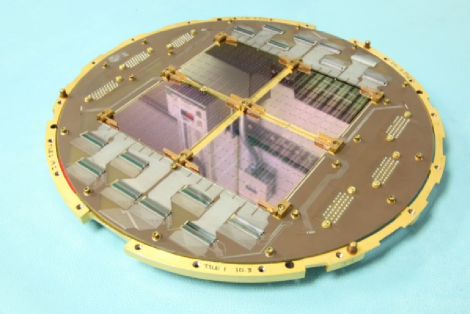
7. Detectors
The focal plane was populated with integrated arrays of antenna-coupled bolometers. This technology combines beam-defining planar slot antennas, inline frequency-selective filters, and TES detectors into a single monolithic package. The JPL Microdevices Laboratory produces these devices in the form of square silicon tiles, each containing an array of dual-polarization spatial pixels (64 detector pairs or 128 individual bolometers). The Bicep2 focal plane had four of these tiles, for a total of 500 optically coupled detectors and 12 dark (no antenna) TES detectors. The detector tiles were characterized at Caltech and JPL during 2008–2009. The rapid fabrication cycle of the Caltech-JPL detectors made it possible to incorporate results of pre-deployment testing into the final set of four tiles deployed in Bicep2. Further details of the detector design and fabrication will be presented in the Detector Paper, which will report on improvements to the detector tiles leading up to Bicep2 as well as further developments in subsequent generations informed by Bicep2 testing.
 |
 |
7.1. Antenna networks
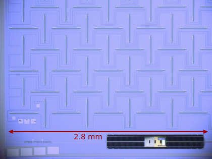
Optical power coupled to each detector through an integrated planar phased-array antenna. The sub-radiators of the array were slot dipoles etched into a superconducting Nb ground plane. The two linear polarization modes were received through two orthogonal, but co-located, sets of 288 slots (for a total of 576 slot-dipoles per dual-polarization spatial pixel). Since the tiles were mounted in the focal plane with the detector side down, the antennas received power through the silicon substrate. A Nb backshort reflected the back-lobe in the vacuum half-space behind the focal plane. The design of the slot antennas has gone through many iterations. The final design used in Bicep2, called the “H” antenna after the arrangement of horizontal and vertical slots (Fig. 8), has exceptionally low cross-polar responses over fractional bandwidth (kuo08).
Currents induced around the slots coupled to planar microstrip lines integrated onto the backside of the antenna arrays. The waves from the sub-radiators summed coherently in a corporate feed network that accomplished the beam synthesis traditionally handled by a feed horn. Two interleaved feed networks independently summed the two polarizations before terminating at two different detectors. Each pixel’s antennas were on a side, matching the optics such that the antenna sidelobes terminated on the aperture stop or blackened surfaces inside the telescope tube.
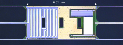
7.2. Band-defining filters
Each microstrip feed-network contained an integrated filter (Fig. 7) to define a frequency band centered at and with 25% fractional bandwidth (defined at the 3 dB points). The 3-pole filter contained lumped inductors made from short lengths of coplanar waveguide. Each of the three inductors coupled to its neighbor through a T-network of capacitors. The achieved bands are characterized in §10.1.
The band-defining filter was omitted in twelve detectors of the array to create dark TESs with no connection to the antennas. These were used to characterize sensitivity to signals such as temperature fluctuations and RF interference.
7.3. TES bolometers
After passing through the band-defining filter, microwave power was carried to a strip of lossy gold microstrip line on a released bolometer island (Fig. 10). The power thermalized in the gold resistor, heating the low-stress silicon nitride (LSN) island. The island was held by narrow LSN legs that formed a thermal weak link to the rest of the focal plane with thermal conductance . The leg conductivity was tuned (orlando10; obrient12) to optimize the noise and saturation power, as described in §10.3.
Each LSN island contained two TES detectors that changed in current in response to changes in the temperature of the island. A primary, titanium TES was designed to operate under low loading conditions when observing the sky, with transition temperature () of –. A second, aluminum TES was placed in series with the primary TES. The Al TES had a higher and higher saturation power for use in the laboratory or when observing mast-mounted sources. The sensitivity of the experiment depends crucially on the performance of the detectors. Their optimization and characterization are reported in detail in Section 10.
7.4. Direct island coupling and mitigation
In pre-deployment tests an earlier generation of detectors showed an unexpected, small coupling to frequencies just above the intended band. The out-of-band power detected was typically 3-4% of the total response and had a wide angular response. We interpreted this response as power coupling directly to the bolometer island. This was reduced in the deployed Bicep2 detectors through the addition of the metal mesh low-pass edge filter to the optics stack (§4.3) and several design changes described in more detail in the Detector Paper. We changed the leg design to reduce the width of the opening in the ground plane around the island and metalized the four outer support legs with Nb to reduce the RF impedance to the island ground plane. The dark island coupling was reduced to 0.3% of the antenna response in the experiment as deployed.
7.5. Device yield
Initial electrical testing of detector arrays checked for continuity across the devices, with correct room-temperature resistance and no shorts. This fabrication yield was extremely high, 99% for the four tiles in Bicep2. When the detectors were integrated into the focal plane and telescope there were additional losses from open lines in the readout, further reducing the overall yield to 82%. The remaining 412 “good light detectors” are those that were optically coupled and had stable bias and working SQUID readout. A detector has been included in this count only if both it and its polarization partner satisfy the same criteria. The number is reduced somewhat in analysis by data quality cuts on beam shape and noise properties as described in §13.7.
8. Cryogenic and thermal architecture
8.1. Cryostat
The telescope was housed within a Redstone Aerospace101010Redstone Aerospace, Longmont, CO 80501, http://www.redstoneaerospace.com/ liquid-helium cooled cryostat that was very similar to the Bicep1 dewar. The major change was that the liquid nitrogen stage of Bicep1 was replaced with two nested vapor-cooled shields, so that liquid helium was the only consumable cryogen. The helium reservoir had a capacity of 100 L and consumed about 22 L/day during ordinary observing.
8.2. Refrigerator
The detectors were operated at 270 mK in order to achieve photon-noise-limited sensitivity. Our focal plane and surrounding intermediate temperature components were cooled using a closed-cycle, three-stage (4He/3He/3He) sorption refrigerator (duband99). The intermediate 3He stage provided a 350 mK temperature used to heat-sink the niobium magnetic shield (§5.3), while the final 3He stage provided a 250 mK base temperature. The initial condensation of the 4He stage was performed by closing a heat switch to thermally couple the fridge to the cryostat’s liquid helium reservoir. The condensed liquid was then pumped by a charcoal sorption pump to pre-cool the next stage.
The refrigerator had an enthalpy of 15 J at the intermediate 350 mK stage, and 1.5 J at the 250 mK stage. The carbon-fiber truss structures (§5.1), along with other aspects of the thermal design, yielded very low parasitic thermal loads. The refrigerator was able to provide a stable base temperature for more than 72 hours. After the liquid reservoirs were exhausted, they were replenished from the charcoal by performing a five-hour regeneration cycle. In order to allow for a margin of safety and align with the Bicep2 observing pattern, we recycled the refrigerator once within each observing schedule of three sidereal days, as described in Section 12.3.
8.3. Thermal architecture and temperature control
Several improvements were made in the thermal path between the refrigerator and the focal plane relative to Bicep1, giving Bicep2 improved stability and reduced vibrational pickup. The coldest stage of the refrigerator was linked to the focal plane through a thermal strap and a passive thermal filter. The thermal strap was designed as a flexible stack of many layers of high-conductivity Cu foil, which reduces the vibrational sensitivity relative to the stiffer linkages used in Bicep1. The passive thermal filter was a rectangular stainless steel block, in length and with a cross-section. The design approach for the passive filter was inspired by the distributed thermal filter used in the Planck HFI instrument (planck03spie; planckfilter). The filter had high heat capacity and low thermal diffusivity in order to achieve adequate thermal conduction with a sufficiently long time constant. Stainless steel (316 alloy) was chosen as a readily available material with suitable thermal and magnetic properties, though other materials, such as holmium, have lower thermal diffusivity. The filter effectively isolated the focal plane from thermal fluctuations on time scales shorter than about .
With no additional heating, the focal plane achieved a base temperature of 250 mK. Temperature control modules (TCMs) consisting of two NTD thermometers and one resistive heater were employed in a feedback loop to control the temperature of the focal plane and the fridge side of the thermal filter (as shown in Fig. 5) to 280 and 272 mK respectively, well below the titanium TES transition temperature. Temperature stability of the tile substrates was monitored using NTD thermometers mounted on each detector tile and by dark TESs on the detector tiles. The tile NTD data have been used to demonstrate that the achieved thermal stability met the requirements of the experiment (§11.7).
Temperatures were also monitored at critical points using Cernox resistive sensors111111Lake Shore Cryotronics, Inc., Westerville, OH 43082, http://www.lakeshore.com/ and/or diode thermometers.
8.4. Housekeeping
The AC signals from the NTD thermometers (rieke89) were read out using junction gate field-effect transistors that are housed at the stage (although self-heated to ) to reduce readout noise (spirejfet). The NTD thermometers were read out differentially with respect to fixed-value resistors, also cold, and each biased separately. Resistor heaters provided control of the sorption fridge, a heat source for temperature control of the cold stage, and instrument diagnostics.
The warm housekeeping electronics were composed of two parts: a small “backpack” that attached directly to the vacuum shell of the cryostat (Fig. LABEL:fig:mount) and a rack-mounted “BLAST bus” adapted from the University of Toronto BLAST system (wiebethesis). The backpack contained preamplifiers for readout channels and the digital-analog converters (DACs) for temperature control and NTD bias generation, all completely enclosed within a Faraday-cage conducting box. The BLAST bus contained the analog-digital converters (ADCs) themselves, as well as digital components for the generation of the NTD bias signals and in-phase readout of the NTDs. This split scheme was designed to isolate the thermometry signals as much as possible from pickup of ambient noise while keeping the backpack small enough to fit within the limited space behind the scanning telescope.
The housekeeping system was upgraded after the first year of observing in order to improve the noise performance of the NTD readout. The upgraded firmware allowed more effective use of the fixed resistors as a nulling circuit to maximize the signal while maintaining linearity in response. The frequency of the NTD bias was also increased from to to improve noise performance.
9. Data acquisition system
Bicep2 used a multiplexed SQUID readout that allowed it to operate a large number of detectors with low readout noise and acceptably low heat load from the wiring. We describe the NIST SQUIDs and other cold hardware, the room-temperature Multi-Channel-Electronics (MCE) system, and the custom control software that were used for data acquisition.
9.1. Multiplexed SQUID readout
Bicep2 used the “MUX07a” model of cryogenic SQUID readout electronics provided by NIST (dekorte03). These were designed for time-domain multiplexing (chervenak99; irwin02), in which groups of 33 channels are read out in succession through a common amplifier chain. This scheme supports large channel counts with a small number of physical wires so that the heat load on the cold stages remains low.
Each detector had its own first-stage SQUID, and the 33 first-stage SQUIDs in one multiplexing column were coupled to a single second-stage SQUID through a summing coil. The first- and second-stage SQUIDs for one column of detectors were packaged together into a single multiplexing (MUX) integrated circuit chip. A second chip, the Nyquist chip, contains the TES biasing circuitry, including a 3 m shunt resistor to supply a voltage bias for the 60 m TES and a 1.35 H inductor to limit the detector bandwidth. Both the MUX and Nyquist chips were bonded to alumina carriers and mounted to the focal plane PCB layer (Fig. 6 right-hand panel; Fig. 5.3). The PCB was connected to Nb/Ti twisted pair cables running to the stage, where SQUID series arrays (SSAs) were used for impedance matching to room-temperature amplifiers. This entire chain was operated in a flux-locked-loop mode by applying a feedback signal to the first-stage SQUIDs. This feedback ensured that all SQUIDs operated very near their selected lock points and maintained constant closed-loop gain.
| 2010 | 2011–12 | |
| Raw ADC sample rate | 50 MHz | 50 MHz |
| Row dwell | 98 samples | 60 samples |
| Row switching rate | 510 kHz | 833 kHz |
| Number of rows | 33 | 33 |
| Same-row revisit rate | 15.46 kHz | 25.25 kHz |
| Internal downsample | 150 | 140 |
| Output data rate per channel | 103 Hz | 180 Hz |
| Software downsample | 5 | 9 |
| Archived data rate | 20.6 Hz | 20.0 Hz |
The SQUIDs and associated hardware are sensitive to ambient magnetic signals. This sensitivity was reduced by the gradiometric design of the first-stage SQUIDs and further attenuated through magnetic shielding (§5.3), but the MUX07a model was particularly susceptible to pickup at the first-stage SQUID (stiehl11). The multiplexed readout is also susceptible to several types of inter-channel crosstalk (§11.5), although development of the NIST hardware over several generations has greatly reduced these effects.
9.2. Warm multiplexing hardware
The warm electronics for detector bias and multiplexed readout were the Multi-Channel Electronics (MCE) system developed by the University of British Columbia (mce08) to work with the NIST cold electronics. The MCE is a 6U crate that was attached to a vacuum bulkhead at the bottom of the cryostat as in Fig. LABEL:fig:mount. It interfaced to the cold electronics through three RF-filtered 100-pin micro-D metal (MDM) connectors and communicates with the control computers through two optical fibers (selected for their high data rates and electrical isolation). A third optical fiber connected the MCE to an external synchronizing clock (“sync box”), which provided digital time stamps used to keep the bolometer time streams precisely matched to mount pointing and other data streams (see Section 9.4).
9.3. Multiplexing rate
The multiplexing rate was chosen to read out each detector frequently enough to avoid noise aliasing while also waiting long enough between row switches to avoid settling-time transients that could cause crosstalk.
Avoiding noise aliasing requires the readout rate to be sufficiently above the knee frequency of the circuit formed by the Nyquist inductor and the TES resistance. For our typical device resistance (, see §10.4) and the cutoff frequency is . At initial deployment Bicep2 used a row visit rate of , which kept the level of crosstalk acceptably low but resulted in a significant noise contribution from aliased TES excess noise (§10.7).
Additional studies of crosstalk and multiplexing rate were performed in late 2010, resulting in SQUID tuning parameters that allowed a faster row switching rate of without a significant increase in crosstalk (brevik10). The multiplexing parameters (Table 2) were adopted at the beginning of 2011, with an expected gain of in sensitivity. The actual improvement in sensitivity is discussed in §LABEL:sec:mapspeed.
9.4. Control system
Overall control and data acquisition were handled by a set of Linux computers running the Generic Control Program (GCP), which has been used by many recent ground-based CMB experiments (story12). The Bicep2 version of GCP was based on the Bicep1 code base, with changes to integrate with the MCE hardware and software. It has been further adapted for use in the Keck Array.
GCP provided control and monitoring of almost all components of the experiment, including the telescope mount, focal plane temperature, refrigerators, and detectors. It provided a scripting language used to configure observing schedules (§12.3).
9.5. Digital filtering
The TES detectors themselves had a very fast response, with typical time constants of several milliseconds. Given the scan pattern the band of interest for science lay below (§12.2). In order to conserve bandwidth across the South Pole satellite data relay we downsampled the data to 20 samples per second before archival. This required an appropriate antialiasing filter, which was applied in two stages. The MCE firmware used a fourth-order digital Butterworth filter before downsampling to 100 samples per second. The second stage was in the GCP mediator, which applied an acausal, zero-phase-delay FIR filter before writing data to disk. As these were both digital filters, their transfer functions are precisely known and do not vary. The GCP filter was designed using the Parks-McClellan algorithm (filtpm) with a pass band at times the Nyquist frequency. This Nyquist frequency was set by the desired downsampling factor of (2010 data set) or (2011-12 data set). Both filters were modified at the end of 2010 to accommodate the change from 15 kHz to 25 kHz multiplexing. A small amount of March 2010 data used a more compact FIR filter with larger in-band ripple. This ripple is with the earliest March 2010 settings, with the settings used in the remainder of 2010, and with the 2011–12 settings.
10. Detector performance and optimization
We selected the parameters of the antenna-coupled TES detectors for Bicep2 for low noise to maximize the instantaneous sensitivity of the experiment, while also allowing a margin of safety for stable operation under typical loading conditions. The noise in polarization (i.e. pair-differenced time streams) at low frequency was dominated by photon noise, which was controlled by minimizing sensitivity to bright atmospheric lines (§10.1) and by reducing internal loading (§4.3). The next largest noise component was phonon noise from fluctuations in heat flow between the islands and the substrate. This was kept low by tuning the leg thermal conductance (§10.3). Finally, we tuned the detector bias voltages to minimize aliased excess noise (§10.5).
We extensively characterized the performance of the detector tiles as fabricated, including the optical efficiency (§10.2), detector properties (§10.4), time constants (§10.6), and noise (§10.7). After optimizations during the 2010 season, the array has achieved an overall noise-equivalent temperature (NET) of .
10.1. Frequency response
The optics, antenna network, and lumped-element filters were tuned for a frequency band at with fractional bandwidth. The band was chosen to avoid to the spectral lines of oxygen at and water at (red curve in Fig. 10.1) in order to reduce atmospheric loading, photon noise, and noise from clouds and other fluctuations in the atmospheric brightness.
The achieved bands were characterized using Fourier transform spectroscopy (FTS). Measurements were performed using a specially built Martin-Puplett interferometer (martin82) designed to mount directly to the cryostat window. The spectrometer’s output polarizing grid was attached to a rotation stage, which steered the output beam across the detector array. The stage also included a goniometer, a device for measuring the angular orientation of the stage. The FTS illuminated approximately a 44 grid of detectors per grid pointing, and multiple pointings were combined to create the archival data set. In order to probe measurement systematics, spectra were taken at several boresight rotations and with several FTS configurations. The detector time streams were combined with encoder readings from the mirror stage to produce interferograms, or traces of power as a function of mirror position. The raw interferograms were low-pass filtered, aligned on the white-light fringe (zero path length difference) and Hann-windowed before performing a Fourier transform to give the frequency response . From the for each detector’s maximally illuminated data set we compute its band center, defined as
| (1) |
and its bandwidth, defined as
| (2) |
The Bicep2 array-averaged band center is GHz, and the array-averaged bandwidth is GHz. Using this definition of the bandwidth, this corresponds to a fractional spectral bandwidth of 28.2%. The array-averaged frequency response is in Figure 10.1.
A mismatch between the bandpasses of the two detectors in a pair can cause a difference in gain that introduces a leakage of CMB temperature into polarization. This is not fully corrected by the relative gain calibration (§13.3), which is based on an atmospheric signal with a different frequency spectrum from the CMB. We define the spectral gain mismatch for each detector pair as in bierman11. The array-averaged spectral mismatch is consistent with zero. Because the source is not fully beam-filling, the spectra for each detector vary somewhat with pointing. We have characterized this by calculating the spectral match for several different pointings of the FTS. We find that the pointing-dependent systematic error on the spectral gain mismatch corresponds to a scatter of 1.7%, so that the FTS measurement can only limit the root-mean-square spectral mismatch per pair to be below this level.
Because a randomly distributed spectral mismatch at the level of 1.7% would introduce a significant false polarization, we have carried out additional analysis to ensure that our polarization maps are not contaminated by relative gain mismatch. We apply the deprojection technique described in the Systematics Paper, and we use simulations to show that leakage from relative gain mismatch is suppressed to an acceptably small level.
10.2. Optical efficiency
The optical efficiency is the fraction of input light that the detectors absorb. It is dependent on the losses within the optics, the antennas, the band defining filters and the detectors. Higher optical efficiencies increase the responsivity and the bottom line sensitivity numbers, but also increase the optical loading and the photon noise. For a beam-filling source with a blackbody spectrum, the power deposited on a single-moded polarization-sensitive detector is
| (3) |
where is the optical efficiency, is the Planck blackbody spectrum, and is the detector response in frequency space as defined in §10.1. Here we choose the normalization condition
| (4) |
In the Rayleigh-Jeans limit (), Eq. 3 reduces to
| (5) |
The optical efficiency was measured in the laboratory using a beam-filling, microwave-absorbing load at both room temperature and liquid nitrogen temperature. This end-to-end measurement, including losses from all optics and using bandwidth of 42 GHz, yielded per-detector optical efficiencies as shown in the upper left histogram of Fig. 10.2, with an array average of 38%.
10.3. Thermal conductance tuning
After photon noise, the next largest noise contribution was phonon noise, corresponding to random heat flow between the island and substrate through the isolation legs. The noise-equivalent power (NEP) from this source is proportional to the island temperature and the square root of the leg thermal conductance (see e.g. hiltonirwin2005):
| (6) |
Here is a numerical factor (typically for these devices) accounting for the finite temperature gradient across the isolation legs. Reducing the thermal conductance lowers the phonon noise power and lengthens the detector time constants. It also decreases the detector’s saturation power, the amount of optical loading required to drive the detectors out of transition and into the normal state. If the saturation power is too low, it may not be possible to operate the detectors during all weather conditions. The selection of is thus a balance between the requirements for low noise and sufficient saturation power.
For Bicep2 we expect edoptical loading of during representative weather conditions (§4.3). We chose to make the optical power and Joule power approximately equal. This gave a saturation power of about twice the ordinary optical loading for a safety factor of two, so that the detectors could operate in almost all weather conditions without saturating. We thus required a saturation power of . For a TES bolometer with thermal conductance , the saturation power is given by
| (7) |
With a typical thermal conductance exponent , transition temperature and substrate temperature , this gives a thermal conductance at substrate temperature or at . We have used the latter as the fabrication target for Bicep2 detectors.
10.4. Measured detector properties
| Detector Parameter | Value |
|---|---|
| Optical efficiency, | 38% |
| Normal resistance, | 60–80 m |
| Operating resistance, | 0.75 |
| Saturation power, | 7–15 pW |
| Optical loading, | 4–5.5 pW |
| Thermal conductance, | 80–150 pW/K |
| Transition temperature, | 505–525 mK |
| Thermal conductance exponent, | 2.5 |
The detector properties were measured in the laboratory and on the sky to be close to the design values. Table 3 summarizes these properties. The detectors were fabricated at JPL in two separate batches, and the differences between these two batches account for the majority of the variation in detector properties, particularly the thermal conductance and the saturation power .
The thermal conductance can be measured by taking sensor current-voltage characteristics or “load curves” in which we sweep the bias voltage and measure the output current. This was repeated at several focal plane temperatures to give a measurement of as shown in the upper right panel of Fig. 10.2. We found in the range –, with the detectors on two of the tiles (Tiles 1 and 2) matching the design characteristic of and a higher on the other two tiles (Tiles 3 and 4). The transition temperature was measured from the same load curve data, with –.
Since the saturation power is directly related to the thermal conductance (Eq. 7), the fractional variation in is similar to that in . With the telescope pointed at the center of the CMB observing field at elevation, the saturation power for the light detectors was –.
The contributions of Joule heating power and optical power to the total can be determined by calculating the Joule power from known and (Eq. 7) or by using the dark detectors, which have no optical power. Both techniques show the Bicep2 optical loading to be –, or –.
The optical loading can further be separated into internal loading and atmospheric loading by measuring the saturation power of the detectors with a mirror placed at the aperture. Because the flat mirror reflects some radiation from the filters, lenses, window, and optics tube, the loading in the mirror test is an upper limit on the internal loading. For detectors near the center of the focal plane, where the reflected radiation is low, the mirror test loading is around 2.2 pW or 10 KRJ. This is similar to the 1.89 pW calculated from the optical loading using temperatures and emissivities of the receiver components as described in Section 4.3 and Table 1. Roughly half of Bicep2’s optical loading was from the atmosphere and half from internal loading.
10.5. Detector bias
The choice of TES bias voltage affects the noise level and stability of the detectors and their safety margin before saturation. We have taken noise data at a range of biases under low loading conditions during winter 2010, in order to choose the settings that give the lowest noise and greatest sensitivity. The optimization is described in detail in brevik10.
The optimal bias voltage for a given TES detector depends on its responsivity (i.e. the shape of the transition, or vs. curve, as in Fig. 10.5) and on its noise properties. Fig. 10.5 shows the noise as a function of bias point in the same 2010 noise data set that was used to optimize the TES biases. For Bicep2 detectors the responsivity was highest in the lower portion of the transition, when the fractional resistance . When the detector was very low in the transition, with close to zero, the detector could enter a state of unstable electrothermal feedback. Higher in the transition, the responsivity decreased and the detector could saturate or have a gain that varies with atmospheric temperature. There was a broad region in the middle of the transition with suitably high and stable responsivity.
Some components of noise also depend on the TES bias voltage. The Bicep2 noise data showed TES excess noise (§10.7) aliased into the low-frequency region . The TES excess noise generically increases with increasing transition steepness parameter
| (8) |
For our detectors was largest low in the transition, so the excess noise was minimized and the sensitivity was highest when the bias point was toward the high end.
The 32 TESs in a multiplexing column shared a common bias line, so this optimization was performed column-by-column to maximize the array sensitivity. At the optimal bias some detectors could be saturated (high bias) or unstable (low bias). This was an acceptable price for maximizing the overall sensitivity.
Before the mid-2010 noise data were taken, we used an initial set of biases chosen based on noise data taken during summer, with higher optical loading. These were deliberately chosen to be conservative, with lower bias for greater margin of safety against saturation. We switched to the optimized detector biases on 2010 September 14 and continued to use them throughout the remainder of the three-year data set. They gave an improvement of 10–20% in mapping speed (§LABEL:sec:mapspeed).
10.6. Detector time constants
The TES detectors had a thermal time constant determined only by the heat capacity of the island and the thermal conductance of the legs. The heat capacity was dominated by the electronic heat capacity of the of added gold, . The conductance varied between and (§10.3, §10.4). These combined to give thermal time constants of , with some variation from detector to detector because of nonuniform . The time constants were faster when the detectors were operated in negative electrothermal feedback (hiltonirwin2005), so that the effective time constant for a typical detector was well below the 4 ms thermal time constant.
Because the frequencies of interest for -mode science are much lower, (§12.2), the detector transfer functions are to a good approximation perfectly flat. This holds as long as the detectors were biased sufficiently low in the transition, with a narrow transition (high ) and strong electrothermal feedback. If a detector was near saturation, its time constant would become slower.
We measured the time constants and end-to-end transfer functions of the detectors in special-purpose calibrations during two of the austral summers. The telescope was illuminated with a broad-spectrum noise source chopped by a PIN diode to a square wave. Metal washers were inserted into a sheet of Propozote foam that was placed over the telescope window to scatter the radiation and uniformly illuminate the focal plane. For time constants the data were taken with modulation and no multiplexing, without applying any digital filters. For transfer functions the data were taken with a square wave, applying the MCE and GCP digital filters as in standard observing. (This frequency was chosen to match the modulation of the atmospheric signal in the el nods used for relative gain calibration (§13.3). The resulting transfer functions could then be used to verify that the relative gains from el nods also held within the full science band.) The transfer function data used a standard data-taking configuration including the MCE and GCP filters (§9.5); the detector time streams were Fourier transformed to give the transfer functions. The response of most detectors was fast enough that the results were indistinguishable from the transfer functions of the digital filters applied by the data acquisition system. A small number of detectors were biased high in the transition and as a result had slower transfer functions. These detectors showed faster transfer functions under lower optical loading, so that the time constants measured with the bright noise source represent worst-case performance. The calibration data are shown in Fig. 10.6 for two detectors, one of which had typical fast response, and one of which had a slow response under the bright illumination of the noise source. The typical detectors’ time constants were sufficiently fast that their transfer functions match the model from the MCE and GCP filters to within . These tests were repeated for all detectors using the 2010 and 2011–12 TES bias and filter settings. The distribution of time constants across the array is shown in the lower left panel of Fig. 10.2.
The time constants are relevant not only to the time stream noise and resulting instrumental sensitivity, but also to the systematics budget of the experiment. Our data analysis deconvolves only the digital filters (§13.1). Following the general strategy for systematics control described in §11 we have performed simulations to show that the flatness of the achieved transfer functions, and in particular the consistency between the A and B detectors in a pair, are sufficient to ensure that the small departures from non-ideality do not significantly impact our results. We confirm this conclusion using the difference map (jackknife test) of left-going and right-going scans. These constraints on the contamination of -modes from detector time constants can be found in the Systematics Paper.
10.7. Time stream noise
The noise level in the detectors has been previously documented in brevik10; brevik11. The noise was characterized in special-purpose data taken at a fast readout rate of 400 kHz by skipping the multiplexing step, allowing aliased noise to be studied separately from intrinsic noise at low frequency. Although degree-scale CMB anisotropies correspond to frequencies of 0.05–1 Hz (§12.2), the noise at much higher frequencies can become relevant through aliasing. This was especially true for the 2010 season, which used a slower multiplexing rate of 15 kHz rather than 25 kHz as in 2011–12.
The noise is broken down by component in Figure 10.7, for the 2010 readout settings. At low frequencies it was dominated by photon noise. The NEP from the photon noise was a combination of the Bose and shot noise (see e.g. hiltonirwin2005):
| (9) |
where is the band center, is the fractional bandwidth, and is the photon loading. For 4–5.5 pW of loading, as measured in §10.4, the photon noise contributed 41–56 aW/.
The next largest contribution to noise at low frequencies was the phonon noise from thermal fluctuations across the SiN legs. The NEP contribution (Eq. 6) was 27 aW/. All other noise contributions, such as Johnson and amplifier noise, were subdominant in the low-frequency region.
However, at frequencies of 1 kHz, the TES Johnson noise and the TES excess noise both contributed substantially. The excess noise (galeazzi11) increased at lower TES biases and had a power spectral density similar to Johnson noise. The 15 kHz multiplexing rate used in 2010 (shown as a vertical line in Figure 10.7) aliased that noise into the low-frequency region. The increased multiplexing speed of 25 kHz in 2011–2012 reduced that aliasing amount. The total noise, including aliasing effects, was 67–78 aW/ with 2010 settings and 56–64 aW/ for 2011–12 configuration.
Combining the noise, optical efficiency, optical loading, and yield using the method described in kernasovskiy12, and converting to CMB temperature units, Bicep2 as a whole is predicted to have an NET of 15 K with the 2011–12 settings. The actual detector performance was evaluated using the noise in the range 0.1–2 Hz in a subset of 2012 CMB data, giving 316 K per detector and 15.9 K for the array (brevik11). The per-detector distribution is shown in the lower right histogram of Fig 10.2. The NET as calculated from the time streams agrees well with the results of a separate calculation from coadded maps, which gives 15.8 K.
11. Instrument performance
While the previous section focused on detector properties that affect the sensitivity of the experiment, the instrumental performance characteristics described in this section contribute to the systematics budget. We have extensively measured these characteristics in both pre-deployment tests and post-deployment calibration measurements. The results in this section combine results from laboratory tests, in situ calibrations, and (in some cases) the CMB data set itself.
In general, we have not relied on meeting predetermined benchmarks in these properties to guarantee adequate control of systematics. Instead, we use the results of tests and calibration data as inputs to detailed simulations that we use to calculate the contribution of each effect given the actual performance of Bicep2, its observing pattern and noise levels, and the same analysis pipeline that we use to prepare maps and angular power spectra from real data.
The Systematics Paper will present the set of simulations and the powerful analysis technique of deprojecting instrumental effects. The Beams Paper will apply these same methods to the important class of systematics related to beams. It will present a set of simulations made from observed high signal-to-noise beam maps for each detector, with no assumption of Gaussianity or ideality. In the current paper we describe the calibration measurements including the high-quality beam maps, and note that the simulation campaign has shown that the instrumental performance as reported here meets the requirements for Bicep2 to remain sensitivity limited rather than systematics limited.
11.1. Mast-mounted source calibrations
Many of the calibration measurements at the South Pole involved observation of a millimeter-wave source in the optical far field. We mounted sources on a high mast on the Martin A. Pomerantz Observatory (MAPO) at a distance of from the telescope. The source then appeared at an elevation of about above the horizon as seen from Bicep2. The ground shield and roof penetration did not allow Bicep2 to directly observe at elevations below , so far-field source calibrations were made with the aid of a flat mirror mounted to the front of the telescope. The far-field flat mirror was also used for occasional observations of the Moon and Venus. Because observations of terrestrial and astrophysical compact sources all required the flat mirror to be installed, these measurements could only be made during summer calibration work.
11.2. Beams
The far-field optical response of each detector was measured before and after each observing season at the South Pole. The far-field beam mapping campaign and full beam properties will be presented in the Beams Paper along with simulations that establish stringent limits on the level at which beam systematics enter our -mode results. Here we briefly describe the beam maps used in this analysis and summarize the overall properties of the beams individually and in pair difference.
The characterization of the shape and position of each detector’s beam was performed by mapping the optical response to a chopped thermal source mounted on the MAPO mast (in the optical far field). A chopper wheel modulated between the cold sky ( K) and ambient temperature ( K) at a rate of Hz. This largely unpolarized blackbody source was well suited for measuring the spectrally-averaged optical response of the instrument. The quality of this data set is illustrated in Fig. 11.2, which shows a composite beam map that has been centered and co-added over all operational channels. The Beams Paper will show the results of a set of optical simulations which give a very good match to the observed main beam and Airy ring structure.
We use elliptical Gaussians as a convenient way to parameterize beam shapes in Table 4, although our analysis does not rely on an assumption of Gaussianity. Fig. 11.2 shows an example map of a typical detector, the elliptical Gaussian fit to the beam, and the fractional residual remaining after subtracting the fit. We extract five parameters for each detector: position (in two directions), beam width, and ellipticity (two parameters). Two parameters are required to fully specify ellipticity: these could be ellipticity and orientation, but we use two orthogonal components known as the “plus” and “cross” orientations, which are analogous to Stokes parameters for polarization. These five parameters are defined in terms of the semimajor and semiminor axes and , and the rotation angle of the major axis. Table 4 lists the mean value for each quantity along with the scatter among detectors. The beam width has an average value of with standard deviation of across detectors (). This is close to the predicted by optics simulations (§4).
| Parameter121212The per-detector parameters are calculated as an inverse-variance weighted combination of the elliptical Gaussian fits to 24 beam maps with equal boresight rotation coverage. | Symbol | Definition | Mean131313Mean across all detectors used in science analysis. | Scatter141414Standard deviation across all good detectors. The uncertainty of the measurement for each detector is small compared to the true variation from detector to detector. |
|---|---|---|---|---|
| Beam width | ||||
| Ellipticity Plus () | 0.013 | 0.03 | ||
| Ellipticity Cross () | 0.03 |
| Parameter151515Differential parameters are calculated by differencing measured beam parameters for detectors and within a polarized pair. | Definition | Mean161616Mean across all detector pairs used in science analysis. | Scatter171717Standard deviation across all detector pairs used in science analysis, dominated by true pair-to-pair variation. |
|---|---|---|---|
| Differential Pointing, | |||
| Differential Pointing, | |||
| Differential Beam Width, | |||
| Differential Ellipticity, | 0.016 | ||
| Differential Ellipticity, | 0.014 |
The differential beam parameters for a pair of co-located orthogonally polarized detectors are calculated by taking the difference between the main beam parameters for each detector within the pair. These differential beam parameters are shown in Table 5. The measured differential pointing per pixel for Bicep2 was larger than that observed in Bicep1 and much larger than optical modeling of the telescope predicted (see §4.1). Subsequent detector testing has shown that this differential pointing is related to contamination in the Nb films and crosstalk within the microstrip lines of the antenna array feed networks. Design and fabrication changes described in obrient12 and the upcoming Detector Paper have addressed these two issues to reduce differential pointing for subsequent devices used in the Keck Array and Spider.
The effects of differential pointing, differential beam width, and differential ellipticity have been strongly reduced through the adoption of the deprojection technique described in the Beams and Systematics Papers. We find that no other modes of beam mismatch are present at a sufficiently large level to justify the use of deprojection.
We calculate the ultimate level at which beam imperfections affect our polarization maps by performing simulations with the measured thermal source beam maps as inputs. The simulation pipeline is run with the observed beam map for each detector rather than a Gaussian or other approximation. This technique allows us to include the effects of all possible beam imperfections, not just those that can be represented in terms of the elliptical Gaussian parameters or modes of the deprojection method. We find that the level of contamination from beam shape mismatches is below the noise-limited sensitivity of the experiment.
11.3. Far sidelobes
Far sidelobes of the Bicep2 telescope could potentially see the bright Galactic plane as well as radiation from the ground or nearby buildings. To mitigate far sidelobe contamination in CMB observations, Bicep2 implemented a combined ground shield and forebaffle system (shown in Fig. LABEL:fig:mount) similar to Polar (polar03). The first stage was a large, ground-fixed reflective screen that removed a direct line of sight between the telescope and the ground and redirects any far sidelobes to the cold sky, lowering loading and preventing spurious signals.
The second stage was a co-moving absorptive baffle (keating01) that rotated with the telescope around its boresight and was designed to intercept the farthest off-boresight beams at from beam center. It was constructed from an aluminum cylinder with a rolled lip lined with 10 mm thick sheets of Eccosorb HR. The Eccosorb was coated with Volara foam181818Sekisui Voltek, Lawrence, MA 01843, http://www.sekisuivoltek.com/products/volara.php to prevent snow accumulation and disintegration of the Eccosorb in the Antarctic climate.
The system was designed such that at the lowest CMB observation elevation angle () rays from the telescope must diffract twice (once past each stage of the shielding system) before they hit the ground. This is an identical strategy to Bicep1, described in takahashi10 and shown in Fig. LABEL:fig:mount.
We have two different methods for measuring the far sidelobes: one finds the total power coupling to the detectors from outside the main beam, and the second maps the angular pattern of the sidelobes. Additional information on these measurements can be found in the Beams Paper.
We have used the loading from the absorptive forebaffle as a measure of the total power in far sidelobes. As we removed and reinstalled the forebaffle with the telescope pointed at the zenith, the change in loading per detector corresponded to –. This is higher than the measured Bicep1 value. The origin of this coupling is attributed to a combination of scattering from the foam window, shallow-incidence reflections off the inner wall of the telescope tube, and residual out-of-band coupling (§7.4). The forebaffle loading was highest for pixels located near the center of the focal plane, because these have the largest fraction of their sidelobes terminate on the forebaffle rather than internal surfaces or the sky.
The angular pattern in far sidelobes was mapped using a broad-spectrum noise source with fixed polarization and modulated with a chopper wheel. We made maps at two different levels of source brightness to achieve a high signal-to-noise ratio over a dB dynamic range. This allowed us to measure both the main beam and dim, outlying features without significant gain compression. We found no sharp features in the far sidelobe regime. For a typical detector, less than 0.1% of the total integrated power remained beyond from the main beam.
In order to verify that the total power in far sidelobes matches the integrated power in the angular pattern measured with the broad-spectrum noise source, we made maps of the far sidelobe response with and without the forebaffle installed. The results were consistent with the other far sidelobe measurements. The fractional amount of loading intercepted by the forebaffle averaged across the focal plane was 0.7%, which corresponds to .
11.4. Polarization response
The polarization response of the detectors was measured in two types of calibration tests.
The first technique used a dielectric sheet as described in takahashi10. The dielectric sheet calibrator worked as a partially polarized beam splitter, directing one polarization mode to the cold sky and the orthogonal mode to a warm microwave absorber at ambient temperature (polar03). Because of this temperature contrast, the arrangement acted as a polarized beam-filling source. By rotating the telescope about its boresight beneath this source we obtained a precise measurement of the polarized response of each detector as a function of source angle. This technique was fast and precise but also sensitive to the exact alignment of the calibrator.
The second technique used beam maps of a rotatable polarized broad-spectrum noise source mounted on the MAPO mast (bradfordthesis). To map the response of every detector as a function of polarization angle incident on the detector, we set the polarized source to a given polarization angle and rastered in azimuth over the source over a tight elevation range to obtain beam maps of one physical row of detectors on the focal plane at one polarization angle. We then repeated this measurement in steps of in source polarization angle over a full range. After completing all source polarizations for a given row of detectors, we moved to the next row of detectors and repeated the sequence. We repeated the entire set of measurements at two distinct boresight rotation angles as a consistency check. The response of a single detector to rotation of the polarized source is shown in Fig. 11.4.
Both the dielectric sheet and rotating polarized source calibrators found a very low cross-polar response, . This is consistent with the known level of crosstalk (§11.5) between the two detectors in each polarization pair. The cross-polar response enters the analysis only as a small adjustment to the overall gain of the and polarization, but cannot create any false -mode signal.
The primary -mode target of Bicep2 requires only modest precision in the measurement of the absolute angles of polarization response. We have adopted the per-detector polarization angles from the dielectric sheet calibrator for use in making polarization maps, as they have low statistical error . However, a coherent rotation of polarization angles for all detectors is less strongly constrained because of possible systematics in the alignment and material of the sheet calibrator, and the alignment of the source in the case of the rotating polarized source. We estimate the overall rotation angle from the and correlations of the CMB using a self-calibration procedure (polselfcal). This indicates a coherent rotation of , which is included as an adjustment in the -mode analysis. We also simulate the effect of a similar overall offset to show that the contribution at low is small even for an angle of .
11.5. Crosstalk
The use of a multiplexer in Bicep2 presented several potential sources of crosstalk that did not exist in the single-channel readout used in Bicep1. For a full treatment of the crosstalk mechanisms see dekorte03. The crosstalk arises due to the use of common components for rows or columns of detector in the multiplexer to reduce wiring count and due to the close proximity of magnetically sensitive components.
The largest crosstalk mechanism in Bicep2 was inductive crosstalk between detectors that are nearest neighbors within a multiplexing column, for which first-stage SQUIDs and input coils were in close proximity. A second mechanism was settling-time crosstalk caused by the finite recovery time of the electronics after the multiplexer switched rows. This crosstalk mechanism depends on the dwell time per row. It was extensively tested in 2010 before the increase in readout rate (§9.3) and measured at a level of (2010 settings) or (2011–12 settings).
Crosstalk has been assessed from maps acquired by scanning across both the broad-spectrum noise source and the chopped thermal source. These measurements used the far-field flat mirror and the aluminum transition of the bolometers (which could operate under high loading). The signal-to-noise ratio in these maps was generally adequate to probe crosstalk to a level of around dB. These large-signal beam maps could be sensitive to nonlinear and threshold-dependent crosstalk mechanisms that do not affect standard CMB observations on the titanium transition. We have made a second calculation of crosstalk levels using cosmic ray hits during CMB data taking. When a cosmic ray interacts in a TES island, the deposited energy thermalizes and raises the temperature of the island. This appears as a spike in the time stream exactly as if it were an instantaneous spike in optical power, and is subject to the same forms of crosstalk. We have selected cosmic ray hits of moderate amplitude (equivalent to 15–300 mKCMB), finding around 100 such events per detector in the full data set. We excluded events in which multiple detectors see a large amplitude in order to exclude showers. These were stacked, and the crosstalk level was read from the corresponding samples in all other channels.
The thermal source beam maps show crosstalk at a level of between detectors that are nearest neighbors in the multiplexing sequence. The scatter around the mean is dominated by detector variations; the noise per detector is lower at . The next-nearest neighbors see and all other channels are below the noise level. This is consistent with the 0.25% reported by NIST-Boulder (dekorte03) for an earlier version of the multiplexing chip. This cosmic ray analysis is also consistent with the beam maps, measuring a nearest-neighbor crosstalk level of . This confirms that the crosstalk levels were consistent between the large-signal, aluminum transition data taking mode of the beam maps and the normal CMB data taking mode of small signals on the titanium transition.
Atypical crosstalk between several multiplexer rows was discovered in beam maps taken during instrument commissioning. Single-channel maps showed multiple beams with amplitudes comparable to the expected main beam. The SQUID tunings of the affected channels also showed an unusual flux response. The problem was traced to wiring shorts between the bias lines of several multiplexer rows, which caused first-stage SQUIDs to be inadvertently biased and read out during the wrong part of the multiplexing cycle. This crosstalk was mitigated by reducing the bias levels for the shorting rows until they were low enough to prevent turn-on of multiple SQUIDs at the same time. The affected channels are excluded from mapmaking for the period of time before the fix by channel selection cuts (§13.7).
11.6. Glitches and unstable channels
Whenever the signal in one detector underwent a large step or glitch (usually a cosmic ray hit), there were additional crosstalk considerations beyond the nearest-neighbor mechanisms described in §11.5. There was a coupling to all other channels in the same multiplexing column at a lower level than the nearest-neighbor crosstalk. There was also a coupling to other channels in the same multiplexing row (channels read out at the same time) through the common ground of the ADCs and DACs in the MCE. These mechanisms could introduce small steps in many channels coincident with a glitch or flux jump in a single channel. These are handled conservatively in analysis by deglitching and cutting all channels that might be affected by crosstalk from a glitch event (§13.2).
A small number of channels had readout hardware defects that caused their raw amplifier signal to very frequently undergo spontaneous jumps. A small number of other detectors had unstable TES bias points and sometimes entered a state of electrothermal oscillation. Either class of pathology could cause localized transient signals or step offsets on other detectors in the same multiplexing row and column, which then lost livetime to deglitching (§13.2) and cuts (§13.7). We found that it was useful to disable SQUID flux feedback only for those detectors that showed no optical response in the time streams. For channels that were severely unstable but had some optical response, we kept the feedback servo active to minimize disruption to neighboring channels.
11.7. Thermal stability
Bicep2 maintained a stable focal plane temperature through passive filtering and active thermal control as described in §8. We have measured the performance of both these components to show that the achieved stability met the requirements of the experiment.
To characterize the passive thermal filter, a heater near the sub-kelvin fridge was turned on and off in a square-wave pattern with an amplitude of 7 mK. The frequency of the square wave was varied while temperatures were monitored on the fridge and focal plane sides of the passive thermal filter. The filter’s low-frequency performance (0.1 Hz) can be modeled as a continuous-pole low-pass filter with a characteristic frequency of 0.291 mHz. Measurement of the filter’s response in our science band was limited by crosstalk between the thermometers. The thermal filter suppressed thermal fluctuations originating from the refrigerator by at least a factor of for .
In CMB units, the spurious polarization signal caused by temperature fluctuations is proportional to the matching of in a detector pair, where is the thermal conductance of the bolometer at the base temperature and is the optical efficiency. Because Bicep2 had higher optical efficiency and lower thermal conductance than Bicep1, this ratio was much lower for Bicep2 and the sensitivity to thermal fluctuations was correspondingly reduced. We calculate the required level of thermal stability using simulations with measured detector thermal responsivities, as was done for Bicep1. For a target of = 0.01 we found the required stability is 6.0 nKFPU at . For comparison, Bicep1’s thermal stability benchmark was 3.2 nKFPU for a target of = 0.1 (takahashi10).
To quantify Bicep2’s achieved thermal stability, angular power spectra were calculated from the NTD thermometer channels instead of the TES bolometer channels. These NTD thermometers were not optically coupled and provide a measure of the temperature fluctuations on the focal plane. To produce spectra, the thermometer time streams were processed into maps using the standard analysis pipeline (see §13). The NTD maps are noise-dominated, so they provide only an upper limit on the achieved thermal stability of the experiment. This upper limit gives temperature fluctuations of at , averaged over a year of data. This is well below the requirement. Further details of this calculation can be found in the Systematics Paper.
11.8. Electromagnetic interference
The telescope was sensitive to the signal of the Amundsen-Scott South Pole Station’s S-band uplink to the GOES satellite, which provides seven hours of telephone and network connectivity to the station each day. When the ground station transmitter was powered on it appeared in Bicep2 data as a ground-fixed signal that had a characteristic pattern in azimuth and did not vary strongly with time. The level of sensitivity varied from detector to detector, with most seeing a small signal equivalent to and a few seeing pickup as large as . The amplitude of this signal scaled linearly with the power at the transmitter, and it did not appear in open-input SQUID channels or in tests with unbiased TESs. These results suggest that power from the ground station transmitter was eventually thermalized in the TES island. Further tests with the Keck Array have shown that the 2.0 GHz radiation entered through the window rather than through the electronic feedthroughs on the back of the telescope. We have confirmed that all other frequency bands used for satellite communication at the South Pole have much lower power levels.
Because the signal had a fixed pattern in azimuth, it can be effectively removed from the bulk of our data by the ground-subtraction step in mapmaking. The exceptions are the beginning and end of each satellite pass, when the transmitter changed state during a scan. The pickup signal is largest only when the telescope pointed toward the ground station. The Bicep2 observing schedule and the satellite communications schedule were both based on sidereal time, and they fortuitously aligned such that the telescope always pointed away from the ground station during scheduled GOES communications. The small remaining signal had a negligible impact on CMB maps, as will be shown in the Systematics Paper.
The case is somewhat different for observations of the Galaxy (§12.1). During these parts of the schedule Bicep2 regularly pointed toward the actively transmitting ground station. Past analysis of the Galactic field (as in Bicep1, bierman11) did not use the ground subtraction analysis technique (§13.6). Studies of the Bicep2 Galactic data must therefore ensure that the satellite pickup signal is adequately removed either through cuts, ground template subtraction, or some other technique.
After these transmissions were detected in Bicep2 data, an RF-absorbing barrier was installed on the wall of the GOES radome to attenuate the spillover of power toward the Dark Sector. This will greatly reduce the S-band power incident on the Keck Array and other experiments beginning with the 2014 observing season.
11.9. Pointing
The pointing of the telescope can be analyzed in two parts. The first is the pointing of the central boresight axis of the cryostat, and the second is the pointing of each detector’s beam relative to this axis. The boresight of the telescope was defined as the line in space that remained fixed as the mount rotates in its third axis. All other pointing directions were defined as offsets from the boresight.
The boresight pointing is complicated by the fact that the building sits on a packed-snow foundation over an ice sheet that moves at . The intrinsic precision of the mount and control electronics, combined with the short-term stability of the platform, were sufficient to give blind pointing accuracy below (yoon06). However, the movement and settling of the building caused pointing drifts of 1’ per month. We accounted for these shifts by taking star observations at three boresight angles as often as once every six days (§12.5). The star-pointing data were used to fit a seven-parameter model for the orientation of the mount and the alignment of its axes. In offline data analysis the nearest star pointing fits are used with the pointing model to convert raw archived encoder readings into boresight pointing in horizontal coordinates.
The pointing of each beam relative to the boresight was determined by making temperature maps for each detector as in §13, but omitting the pair difference step. The maps were made separately for each of the four boresight rotation angles, for left-going and right-going scans, for each detector across the 2010–11 data set. Each of these eight maps was then cross-correlated with the temperature map from the five-year WMAP W band data set (wmap5yr). The external temperature map had the WMAP beams deconvolved and was Gaussian-smoothed to the Bicep2 beam size before cross-correlation. The offset that maximized the cross-correlation was taken as a correction to the ideal detector pointing that had been used in forming the single-detector map. From comparison among the eight maps for each detector, we estimate that this procedure gives beam centers accurate to rms. The precision of the fitted beam centers is limited primarily by the step in elevation of the CMB observing pattern, which makes the cross-correlation more weakly sensitive in this direction. We have simulated the effect of cosmological correlations as a bias on the beam centers and find it well below . The same beam-fitting procedure has been repeated with Planck maps (planckI; planckVI) instead of WMAP templates. The results are identical to within for all Bicep2 detectors.
When we compare the beam centers as fit from CMB maps at different boresight rotation angles, we detect an offset in the elevation direction of an average of . We interpret this offset as an internal flexure of the focal plane assembly relative to the cryostat shell and the telescope mount.
12. Observing strategy
The Bicep2 observing strategy was based on deep integration in the region of the sky least contaminated by polarized foregrounds. The telescope spent 90% of its observing time on this CMB field, and the other 10% on a secondary Galactic field. These observations were grouped in schedules of three sidereal days, including a six-hour cryogenic service period. Within one three-day schedule the telescope scanned in azimuth at a fixed boresight angle—the orientation of the telescope about its own axis. The details of the observing schedule were chosen to allow for control of possible systematics such as drift in detector gain and ground-fixed signals.
12.1. Observing fields
Bicep2 spent most of its time observing the primary CMB field centered at (, ). This 1000-degree2 field (2% of the sky) lies well away from the Galactic plane, within a larger region known as the “Southern Hole” where polarized foregrounds are expected to be especially low. The Bicep2 field is the same one observed by Bicep1. It was selected for its very low level of expected Galactic dust emission, less than of the sky median (fds99) as shown in Fig. 12.1. If the dust signal is polarized at 5%, the resulting contamination of the -mode signal at will be below . The faint synchrotron signal within the Southern Hole has not been well measured, but a scaling of WMAP data at implies that the -mode contamination at is at a level similar to or below that from dust (nguyen08).
The secondary Bicep2 field covered a part of the Galactic plane centered at (, ). Observations of this field can be used for Galactic science objectives (bierman11) and as a bright, partially polarized source for use in instrument characterization.
These same two fields have also been observed by Bicep1191919Bicep1 also observed a third field in a different part of the Galactic plane. This field has not been covered by Bicep2 or the Keck Array. and the Keck Array. Coverage of the same fields by the three experiments allows for consistency tests, cross-calibrations on the bright Galactic signal, and the possibility of achieving greater map depth by stacking CMB maps across multiple experiments. The additional frequencies of Bicep1 and the Keck Array (beginning in the 2014 season) also give spectral information needed to separate any foreground signals from the CMB.
12.2. Scan pattern
The telescope scanned at in azimuth, so that at an elevation of 57.5∘ a signal with frequency (in Hz) corresponds to a multipole . This set the science band for the experiment: 0.05–1 Hz for where the inflationary -mode signal is expected to peak, or for .
Each scan spanned in azimuth, of which the central (77.7% of the duration of the scan) was covered at uniform speed and is used for mapmaking. The region around each turn-around is excluded from CMB analysis. The trajectory of each scan was optimized at the time of Bicep2 deployment for a gain of 4% in the usable, central part of the scan relative to Bicep1. The elevation was kept fixed as the telescope executed 53 round-trip scans over a period of 46 minutes. During this single “scan set” the telescope scanned back and forth within fixed limits in azimuth, rather than continuously tracking the sky. Each scan set was preceded and followed by bracketing calibrations as described in §12.4, bringing the total duration of each scan set up to 50 minutes.
At the end of each 50-minute scan set, the telescope stepped up by in elevation and shifted the azimuth of the scan center to follow the apparent motion of the field on the sky before beginning the next scan set.
This scan pattern deliberately covers a fixed range in azimuth within each 50-minute observing block, rather than a fixed range in right ascension. After 50 minutes the CMB has drifted by relative to the ground. Therefore, any pickup of ground-fixed optical power, the magnetic field of the Earth or nearby structures, scan-fixed thermal fluctuations, or scan-fixed vibrational noise would all appear in the same locations from scan to scan. This allows us to remove these signals using a simple ground-subtraction algorithm (§13.6).
| Phase | LST | Field |
|---|---|---|
| A | Day 0 23:00 | Cryo service |
| B | Day 1 05:30 | CMB (high el) |
| C | Day 1 14:30 | CMB (low el) |
| D | Day 1 23:00 | Galactic |
| E | Day 2 05:30 | CMB (low el) |
| F | Day 2 14:30 | CMB (high el) |
| G | Day 2 23:00 | CMB (variable el) |
| H | Day 3 05:30 | CMB (high / low el) |
| I | Day 3 14:30 | CMB (low / high el) |
12.3. Schedules and boresight angles
A three-day schedule was divided into groups of 50-minute scan sets. Each of these groups, called an observing phase, contained ten scan sets (nine hours total) or seven scan sets (six hours total) along with the accompanying calibrations. During one full three-day schedule the telescope completed one six-hour cryogenic service phase, six 9-hour phases and one 6-hour phase on the CMB field, and one 6-hour phase on the Galactic field, as listed in Table 6. The azimuth/elevation pattern of a typical observing schedule is shown in Fig. 12.2. This represents only one of several possible patterns: the Galactic phases alternated among four different elevation ranges; the six-hour CMB phase on day two alternated among low, middle, and high elevation ranges; and the day-three CMB phases alternated between following the day-one pattern (high then low) and the day-two pattern (low then high). These alternations ensured even coverage of each field and uniform coverage of the CMB field at each azimuth range. The low-elevation CMB phases had boresight pointings from to , and the high-elevation CMB phases had boresight pointings from to .
The three-day observing pattern was made possible by the long hold time of the Bicep2 helium bath and 3He sorption fridge; in contrast, Bicep1 and the Keck Array have required cryogenic service every two days. The Bicep2 cryogenic service period was used to refill the liquid helium bath, cycle the sorption fridge, perform star observations to measure telescope pointing, and carry out other maintenance tasks such as cleaning snow from the forebaffle and other exposed parts of the telescope.
Each schedule was taken with a fixed orientation around its axis or boresight angle. We have selected four boresight angles for standard observations:202020A small amount of early Bicep2 data from March 2010 used a different set of four boresight angles, with the same pattern but offset from the final four. These were , , , and . , , , and . These include two pairs separated by , so that it was possible to measure both Stokes and using either + or +. Each of these angles also had a counterpart that is away for characterization and control of instrument systematics such as differential pointing. The boresight angles are defined such that at the A detectors are sensitive to vertical polarization and the B detectors to horizontal polarization, and vice versa at .
12.4. Integrated calibrations
Each 50-minute observing block began and ended with two types of integrated calibrations: an elevation nod (el nod) and a partial load curve. The elevation nod measured detector response to a small change in atmospheric loading as the telescope moved by a small amount in elevation. The response to the el nod gave a measure of the detector response to a change in fractional air mass. This responsivity measure was used for three purposes: 1) to determine the relative gains of the two polarization channels within a pixel, to allow pair differencing; 2) to correct for gain differences between pixels before making maps; and 3) to reject data in which responsivity is anomalous or unstable. The el nod was the only source of gain calibration applied to individual detector time streams; there was no calibration on an astrophysical source until the final absolute calibration, derived from the CMB temperature anisotropy. The details of the gain calibration are presented in §13.3, including an accounting for differences between the atmospheric and CMB spectral energy densities.
In an “up-down-up” el nod, as performed at the start of the observation, the telescope first stepped upward by , then downward by , and upward again by to return to the starting position. This motion was performed slowly over about one minute. The el nod immediately following an observing block was performed in the opposite order, “down-up-down”.
The second type of integrated calibration was a partial load curve. The TESs were first driven normal (heated above their superconducting transition) and the bias voltage as then stepped down to the standard operating point. This gave an - characteristic for each sensor from which we can calculate the optical loading, resistance in the operating and normal state, and Joule heating power. The partial load curves were used to reject data from periods of time when loading conditions placed the detectors outside the regime of linear response, such as unusually cloudy days with very high atmospheric loading.
Extended versions of the el nod and partial load curve were done at the beginning of each phase. The elevation nod was replaced with a sky dip, in which the telescope slewed from an elevation of up to the zenith and back down. This provided a profile of atmospheric conditions. The partial load curve was replaced with a full load curve that covered the range from the high-bias normal state down to the superconducting state at zero TES bias. This gave a complete - characteristic including the entire transition region. The full load curve was performed only once per phase because of the additional time required to put the detectors back on transition from the superconducting state.
12.5. Star pointing
An optical camera was mounted at the top of the cryostat for star observations. The camera has been described in yoon06. The star pointing routine was performed as often as possible in order to measure and correct for the settling of the DSL building on the moving ice sheet. Winter star pointings observed 24 stars, each at three boresight rotations. They were performed every six days except when overcast weather made it impossible to see the stars. Star pointings were also performed in summer; the optical camera was sensitive in the IR, so that it was possible to observe the brightest 12 stars on the list even when the Sun was above the horizon.
The star observations were used to fit a pointing model with seven parameters: the zero points of the azimuth and elevation encoders; the tilt of the azimuth axis in two directions; the tilt of the elevation axis; and two parameters for the collimation of the optical camera relative to the telescope boresight. This pointing model is applied to CMB observations to transform the raw encoder coordinates into azimuth and elevation of the telescope boresight (§11.9).
13. Data reduction
Data reduction is performed using the analysis pipeline developed for the QUaD experiment (pryke09) and subsequently adapted for Bicep1 and Bicep2. In this section we briefly review the data analysis process, focusing on steps that relate closely to the performance of the instrument and the production of the sensitivity figures that will be presented in §LABEL:sec:data. These are primarily the low-level reduction and data quality cuts. The mapmaking procedure, / separation, angular power spectrum analysis, and simulation pipeline are described in detail in the Results Paper and the deprojection algorithm is presented in the Systematics Paper.
13.1. Transfer function correction
As the first stage of low-level data reduction the pipeline deconvolves the filters that have been applied to the time streams (§9.5). The deconvolution kernel is an FIR filter designed from the known transfer functions of the MCE and GCP filters. We choose an FIR filter in order to ensure that any ringing from transients vanishes after a suitably short time. This property allows the deglitching operation (§13.2) to fully remove the effects of glitches and flux jumps while excising only a small amount of data, per event. The deconvolution kernel also includes a low-pass filter component to attenuate signals that could be aliased during mapmaking.
13.2. Deglitching
There are several types of time stream glitches that must be flagged and removed in low-level data reduction. It is necessary both to prevent the glitches themselves from being included in the maps and to ensure that the time streams contain only well-behaved, stationary noise that can be represented by the noise model used in simulations. The majority of glitches in otherwise good channels were caused by cosmic ray hits in the TES islands. The energy deposited by ionization in the substrate thermalized and appeared as a brief spike of power. These transient events can be simply cut from the time streams. We also observe occasional step discontinuities in the DC levels when a cosmic ray event exceeded the bandwidth of the flux-feedback loop and caused it to relock at a different point. These events are very large steps equivalent to . The deglitching code for Bicep2 flags these events for additional correction.
In any given good detector, cosmic ray hits caused transient spikes large enough to be deglitched at about one event per and flux jumps at one per . A small number of channels either had unstable detector bias or readout faults that caused more frequent flux jumps (§11.6).
The time stream around any glitch is cut for before and after the glitch. This time is calculated from the length of the FIR deconvolution kernel (§13.1) to ensure that the remaining time stream can safely be deconvolved without being affected by ringing. For step-like glitches, the DC levels of the time stream before and after the excised portion are level-matched in order to remove the low-frequency Fourier components of the step that could otherwise contaminate noise simulations. Finally, for large flux-jump steps, these measures are applied not only to the affected channel itself, but to all nearby channels that could potentially be sensitive to crosstalk from the affected channel.
13.3. Gain calibration
The gain calibration is performed in two steps. The first is a relative gain calibration derived from elevation nods (§12.4). The second is an absolute calibration derived from the CMB temperature itself and applied in mapmaking. Given the fast detector time constants (§10.6) there is no need for a frequency-dependent gain calibration.
The relative gain calibration is based on the detector response to the el nods performed immediately before and after each observing block. The calibration factor for a given detector is its own el nod response in raw digitizer units per air mass, divided by the median across all detectors on the focal plane. This procedure corrects for variation and drift in individual detector response, while dividing out day-to-day changes in the overall brightness of the atmosphere. The relative gain correction is performed on the time streams as part of the low-level reduction, before the polarization partner channels are combined to give the pair-sum and pair-difference quantities.
The relative gain procedure allows the maps from all detector pairs to be coadded in the same units. This fully integrated map still must be converted into physical units of . We find the absolute gain factor for the entire data set by cross-calibrating the Bicep2 temperature maps against an external data set. The overall intensity calibration thus comes from the CMB itself. The absolute calibration factor is the ratio of two cross-spectra formed from the Bicep2 temperature map and two external data sets, the reference and calibration maps. It is defined in the multipole bin as
| (10) |
We choose to use separate reference and calibration maps, with uncorrelated noise, so that the cross-spectra in the numerator and the denominator of Eq. 10 are both free of noise bias. The resulting calibration is only very weakly sensitive to the reference map. Before forming cross-spectra we reobserve each with the Bicep2 observing pattern, pipeline, and averaged beam profile. The consistency of the across all multipole bins therefore also serves as a confirmation of the correctness of the applied beam profile. For the final gain calibration number we take the mean of over five multipole bins in the range .
We consider the calibration of the Bicep2 three-year data set using external maps from both the WMAP 9-year release (wmap9yr) and the Planck 2013 release (planckI; planckVI). For WMAP we use the V and W band products as the reference and calibration maps, respectively. For Planck we use the and products as the reference and calibration maps, respectively. In each case we deconvolve the WMAP or Planck beams before reobserving with Bicep2 parameters. The statistical error on the resulting estimates of is well below 1%, with the overall uncertainty dominated by the choice of calibration map. The calculations from Planck and WMAP9 differ slightly, with WMAP9 about higher than Planck. This corresponds to the disagreement between the two experiments in the amplitude of the CMB spectrum (spergel2013). We adopt a central value of per raw digitizer unit. Given the tension between external calibration data sets this result can be taken to have an uncertainty of , which meets the requirements for absolute temperature calibration of Bicep2.
13.4. Pair difference
In addition to photon noise and the intrinsic noise of the detectors and readout, there is an atmospheric signal. This appears as noise that dominates at low frequency in the power spectrum from a single detector. Because the atmosphere is very unpolarized (hanany03), the noise can be removed by differencing the A and B detectors of each polarization pair. We form pair-differenced quantities for use in making polarization maps, and pair-sum quantities for use in making temperature maps. The pair-sum time streams contain atmospheric noise while the pair-differenced quantities do not, as shown in Fig. 13.4. The CMB maps accordingly have very different noise properties and weaker sensitivity than the CMB and maps, and the mapping speed in is much more strongly affected by weather. Because the primary science goal of Bicep2 is to make a polarization measurement, while the CMB temperature in our field is already measured to high signal-to-noise, the sensitivity and map depth calculations in §LABEL:sec:data will consider only the pair-differenced or polarization quantities.
13.5. Polynomial filtering
We remove remaining atmospheric noise at very low frequencies and residual magnetic pickup by applying a polynomial filter. This is a third-order polynomial subtracted from the time stream of each pair-sum and pair-difference channel for each left-going or right-going scan. It effectively removes very low frequencies or very low multipole moments in the scan direction (i.e. in right ascension).
13.6. Ground subtraction
We perform an additional filtering step to remove any signal that is fixed relative to the ground rather than the sky. We form a template in ground-fixed coordinates for each pair-sum and each pair-difference channel over all the scans in a scanset and subtract this template from the time streams. Because the sky moves relative to the ground by of azimuth or right ascension during the 50 minutes of a scanset, a sky-fixed signal is not strongly filtered. This filtering is accounted for in the power spectrum analysis as described in the Results Paper.
Several types of signal enter into the ground-fixed template: reflections from ground-fixed objects; any magnetic signal not already removed by polynomial filtering; and the satellite transmitter signal (§11.8). There is some evidence of a small atmospheric polarization dependence on the wind direction. Because the winds at the South Pole are steady over long periods of time, this is also effectively removed by ground subtraction.
13.7. Data selection and cuts
| Cut parameter | Total time [10] | Integration [10] | Fraction cut [%] |
|---|---|---|---|
| Before cuts | 36.5 | 14.8 | – |
| Channel cuts | 36.5 | 13.2 | 10.9 |
| Synchronization | 35.3 | 12.7 | 3.1 |
| Deglitching | 33.6 | 10.7 | 13.8 |
| Per-scan noise | 33.6 | 10.7 | |
| Passing channels | 33.3 | 10.7 | 0.22 |
| Manual cut | 33.0 | 10.6 | 0.43 |
| Elevation nod | 31.0 | 9.2 | 9.5 |
| Fractional resistance | 31.0 | 9.2 | 0.16 |
| Skewness | 31.0 | 9.1 | 0.41 |
| Time stream variance | 30.9 | 9.0 | 0.52 |
| Correlated noise | 30.9 | 9.0 | |
| Noise stationarity | 30.7 | 8.9 | 0.64 |
| FPU temperature | 30.6 | 8.9 | 0.20 |
| Passing data | 27.6 | 8.6 | 1.7 |
The data set used for CMB mapmaking begins on 2010 February 15 and continues until 2012 Nov 6. The period from 2011 January 1 through 2011 March 1 is excluded as it was used for special-purpose calibrations and tuning of the 25 kHz data taking parameters.
We have developed a multistage data cut procedure which identifies and removes data that suffers from pathologies related to detectors, multiplexing, thermal control, noise properties, or data acquisition. The goal is to ensure that all data used in mapmaking is taken when the experiment is operating properly and has only stationary, well-behaved noise. We do not explicitly attempt to cut data which is noisier than average. Instead, we apply inverse-variance weighting in mapmaking to form a nearly optimal combination of partial maps made with detectors and time periods that have differing noise levels.
A full list of the cut parameters is shown in Table 7. The statistics listed are cumulative. The first column gives the total time used for mapmaking after applying the named cut and all cuts listed above it. The second column is similar, but multiplies time by number of included detectors to give a measure of the total map integration after applying each round of cuts. The time and integration only give time actually accumulated into maps; they exclude the time spent in elevation nods, scan turnarounds, etc. The integration column includes only detectors contributing to the polarization maps for each observation. The final column shows the fraction of the total exposure that passes the previous cuts but fails the cut named on this line. Because problematic data often fail several cuts, the fraction removed depends on the order in which the cuts are listed. (For reasons of convenience in implementation the pipeline applies some cuts in a different order from that shown in the table.)
Before applying any cuts there are 384 good light channels in the early 2010 data set and 412 in late 2010 through 2012 (after TES bias optimization). The first cut is a channel cut that removes detectors with discrepant beam shape or differences in pointing and beam shape between the A and B detectors. It also removes a small number of detectors in which there is a detectable amount of leakage of unpolarized signal into the pair-differenced time streams because of faults in the multiplexing and readout. After applying channel cuts there are 334 remaining channels in early 2010 and 370 in late 2010 through 2012. The second line of Table 7 shows that the channel cuts do not change the total time, but they do remove of the exposure.
The synchronization cut excludes several discrete periods of time in 2010 and 2011 when the time stamps in the MCE data could not be matched to time stamps in the telescope pointing because of failures in the hardware or control system (§9.4).
Cuts related to deglitching remove individual scans affected by flagged transient events, both for the affected detector and (in the case of large glitches or flux jumps) for neighbors potentially vulnerable to crosstalk. Channels suffering an excessive number of glitches within a scanset are removed for the duration of the scanset. This cut removes a substantial amount of data, primarily because of the necessity of cutting the neighbors of unstable detectors (§11.6). The per-scan noise cut is set very loosely to exclude only severely high noise also likely to be caused by a detector instability.
The passing channels cut requires that each individual scan have a sufficiently large fraction () of detectors within each multiplexing column passing all cuts. This is a further precaution against time stream irregularities that could affect other channels through crosstalk.
The manual cut removes a small amount of data in 2010 that appear nominal but may have nonstandard settings and is removed as a precaution.
The elevation nod cuts ensure that the leading and trailing elevation nods have atmospheric response agreeing to within 30% in each channel, or 10% in the ratio of A to B detectors within a pair. This ensures that the relative gain is sufficiently stable for the pair differencing procedure to remove atmospheric noise. Detectors are also cut if their el nods contain time stream glitches or fail to match the expected atmospheric profile. These cuts primarily remove data in which the atmosphere changes too much over the course of a scanset, for example when clouds are carried in or out by wind.
The fractional resistance cut removes detectors that have fractional resistance outside the range . This excludes detectors that have either latched into the superconducting state or have been pushed out of transition by unusually high atmospheric loading.
The skewness, time stream variance, correlated noise, and noise stationarity cuts remove detectors whose noise does not match the expected model during a scanset. This is usually caused by an irregularity in the readout system or by unusually time-varying weather.
The FPU temperature cut requires that the focal plane Cu plate be stably in the range – with a standard deviation no more than . This removes a small number of scansets in which the temperature had not settled sufficiently after the refrigerator recycling.
Finally, we demand a reasonable fraction of data to pass all of the above cuts. This passing data cut ensures that the experiment is generally performing as expected during a particular scan set. If fewer than 50% of channels pass all the cuts, then the all of the data for that scanset is removed.
The overall pass fraction of the cuts is 75.6% in terms of integration time, or 58.1% in terms of exposure when accounting for the number of detectors passing cuts in each scanset. The bottom-line figures in Table 7 give an average detector count of individual detectors contributing to the map at any given time.
13.8. Mapmaking
The time streams are binned into equirectangular maps on a grid in right ascension and declination. The map pixels are square at the center of the field, declination . The pair-sum time streams are accumulated into the map, while the pair-difference time streams are accumulated into the and maps according to the polarization angles of the detectors as transformed into celestial coordinates. As the time stream for a single detector pair in a single scanset is coadded into the map, it is weighted according to the inverse of its time-stream variance across the entire scanset.
We ordinarily apply deprojection of one or more templates during mapmaking in order to remove modes that have been contaminated by mismatches between the A and B beams or relative gains. The deprojection algorithm and its effectiveness are described in the Systematics Paper. For the remainder of the current paper we apply deprojection of relative gain mismatch, differential pointing, and differential ellipticity.