On extremals of the entropy production by “Langevin–Kramers” dynamics

Abstract

We refer as “Langevin–Kramers” dynamics to a class of stochastic differential systems exhibiting a degenerate “metriplectic” structure. This means that the drift field can be decomposed into a symplectic and a gradient-like component with respect to a pseudo-metric tensor associated to random fluctuations affecting increments of only a sub-set of the degrees of freedom. Systems in this class are often encountered in applications as elementary models of Hamiltonian dynamics in an heat bath eventually relaxing to a Boltzmann steady state.

Entropy production control in Langevin–Kramers models differs from the now well-understood case of Langevin–Smoluchowski dynamics for two reasons. First, the definition of entropy production stemming from fluctuation theorems specifies a cost functional which does not act coercively on all degrees of freedom of control protocols. Second, the presence of a symplectic structure imposes a non-local constraint on the class of admissible controls. Using Pontryagin control theory and restricting the attention to additive noise, we show that smooth protocols attaining extremal values of the entropy production appear generically in continuous parametric families as a consequence of a trade-off between smoothness of the admissible protocols and non-coercivity of the cost functional. Uniqueness is, however, always recovered in the over-damped limit as extremal equations reduce at leading order to the Monge–Ampère–Kantorovich optimal mass transport equations.

1 Introduction

The contrivance and development of techniques that can be used to investigate the physics of very small system is currently attracting great interest [1]. Examples of very small system are bio-molecular machines consisting of few or, in some cases, even one molecule. These systems are able to “efficiently”, in some sense, operate in non-equilibrium environments strongly affected by thermal fluctuations [2]. For example, protein biosynthesis relies on the quality and efficiency with which the ribosome, a complex molecular machine, is able to pair mRNA codons with matching tRNA. During such process, known as “decoding”, the ribosome and tRNA undergo large conformation changes which appear to correspond to an optimal in energy landscape recognition strategy [3].

One relevant motivation for attaining a precise characterizations of thermodynamic efficiency of single-biomolecule systems such as molecular switches is the hope that their properties can be exploited in molecular-scale information processing [4]. A long-standing conjecture by Landauer [5] surmises that the erasure of information is a dissipative process. Brownian computers [4] incorporate this conjecture in the form of models amenable to experimental [6] and theoretical [7] investigation. In particular, the erasure of one bit of information can be modeled by steering the evolution of the probability density of a diffusion process in a bistable potential by manipulating the height and the depth of the potential wells [4]. Using the optimal control techniques introduced in the context of stochastic thermodynamics by [8, 9], the authors of [7] (see also [10]) showed that the minimal average heat release during the erasure of one bit of information generically exceeds Landauer’s $k_{\mathrm{B}}\,\beta^{-1}\ln 2$ bound where $\beta$ is the inverse temperature and $k_{\mathrm{B}}$ Boltzmann’s constant. This theoretical result is consistent with the experimental findings of [6] where one bit erasure was modeled by a system of a single colloidal particle trapped in a modulated double-well potential.

The generality of Landauer’s argument upholding an ultimate physical limit of irreversible computation and the existence of the recent experimental supporting evidences indicate that the conclusions of [7] should remain true for Markov models more general than Langevin–Smoluchowski’s dynamics. This intuition is corroborated by the fact that the entropy produced by smoothly evolving the probability distribution of Markov jump processes between two assigned states is also subject to an analogous lower bound [11]. The scope of the present contribution is to explore minimal entropy production transitions of continuous Markov processes governed by kinematic laws comprising a dissipative and a symplectic, conservative, component. The consideration of such systems, commonly referred to as Langevin–Kramers or under-damped, is important as they provide models of Newtonian mechanics in a heat bath.

The structure of the paper is as follows. In section 2 we describe the kinematic properties of a Langevin–Kramers diffusion. We also define the class $\mathbb{A}$ of admissible Hamiltonians governing the Langevin–Kramers dynamics to which we restrict our attention while considering the optimal control problem for the entropy production. From the mathematical slant, it is obvious that an optimal control problem is well-posed if we assign besides the “cost functional” to be minimized, the functional space of admissible controls. From the physics point of view, our aim is to explicitly restrict the attention to “macroscopic” control protocols modeled by smooth Hamiltonians acting on “slower” time scales as opposed to configurational degrees of freedom subject to Brownian forces and fluctuating at the fastest time-scales in the model [12] (see also discussion in [11]).

In section 3 we briefly recall the stochastic thermodynamics of Langevin–Kramers diffusions drawing on [13, 14]. The main result is the expression of the entropy production $\mathcal{E}_{t_{\mathrm{f}},t_{\mathrm{o}}}$ over a finite control horizon $[t_{\mathrm{o}},t_{\mathrm{f}}]$ in terms of the current velocity of the Langevin–Kramers diffusion process. As in the Langevin–Smoluchowski case [15, 9, 16], the current velocity parametrization plays a substantive role in unveiling the properties of the entropy production from both the thermodynamic and the control point of view. In the Langevin–Kramers case, the entropy production turns out to be a non-coercive [17] cost functional. Namely, the decomposition of the current velocity into dissipative and symplectic components evinces that the entropy production is in fact a quadratic functional of the dissipative component alone. The origin of the phenomenon is better understood by revisiting the probabilistic interpretation of the entropy production which we do in section 4. There we recall that $\mathcal{E}_{t_{\mathrm{f}},t_{\mathrm{o}}}$ coincides with the Kullback–Leibler divergence $\mathrm{K}(\mathrm{P}_{\chi}||\mathrm{P}_{\tilde{\chi}})$ [18] between the probability measure $\mathrm{P}_{\chi}$ of the primary Langevin–Kramers process $\chi$ and that $\mathrm{P}_{\tilde{\chi}}$ of a process $\tilde{\chi}$ obtained from the former by inverting the sign of the dissipative component of the drift and evolving in the opposite time direction. The Kullback–Leibler divergence is a relative entropy measuring the information loss occasioned when $\mathrm{P}_{\tilde{\chi}}$ is used to approximate $\mathrm{P}_{\chi}$. These facts substantiate, on the one hand, the identification of the entropy production as a natural indicator of the irreversibility of a physical process and, as such, as the embodiment of the second law of thermodynamics. On the other hand, they pinpoint that the interpretation of the entropy production as a Kullback–Leibler divergence is possible in the Kramers–Langevin case only by applying in the construction of the auxiliary process $\tilde{\chi}$ a different time reversal operation than in the Langevin–Smoluchowski case. Non-coercivity is the result of such time reversal operation.

The consequences of non-coercivity of the cost functional on the entropy production optimal control are, however, tempered by the regularity requirements imposed on the class $\mathbb{A}$ of admissible Hamiltonians. Simple considerations (section 5) based on smoothness of the evolution show that the Langevin–Kramers entropy production must be bounded from below by the entropy production generated by an optimally controlled Langevin–Smoluchowski diffusion connecting in the same horizon the configuration space marginals of the initial and final phase space probability densities. This result motivates the analysis of section 6 where we avail us of Pontryagin’s maximum principle to directly investigate extremals of the entropy production in a finite time transition between assigned states. Pontryagin’s maximum principle is formulated in terms of Lagrange multipliers acting as conjugate “momentum” variables (see e.g. [19, 20, 21]). We can therefore construe it as an “Hamiltonian formulation” of Bellman’s optimal control theory which is based upon dynamic programming equations (see e.g. [17, 22, 23]). Relying on Pontryagin’s maximum principle we conveniently arrive at the first main finding of the present paper encapsulated in the extremal equations (54). On the space $\mathbb{A}$ of admissible control Hamiltonians the entropy production generically attains an highly degenerate minimum value. A distinctive feature of the extremal equations (54) is that the coupling between the dynamic programming equation and the Fokker–Planck equation takes the non-local form of a third auxiliary equation. We attribute the occurrence of a non-local coupling to the divergenceless component of the Langevin–Kramers drift.

We illustrate these results in section 7 where we consider the explicitly solvable case of Gaussian statistics. While considering this example, we also inquire the recovery in the over-damped limit of the expression of the minimal entropy production by Langevin–Smoluchowski diffusions, a problem to which we systematically turn in section 8. There we derive our second main result: upon applying a multi-scale (homogenization) asymptotic analysis [24, 25] we show that the cell problem associated to the extremal equations (54) takes the form of a Monge–Ampère–Kantorovich mass transport problem [26] for configuration space marginals of the phase space probability densities. The noteworthy aspect of this result is that the degeneracy of the extremals (54) does not appear in the cell problem so that consistence with the results obtained for Langevin–Smoluchowski diffusions [7] is guaranteed.

Finally, the last section 9 is devoted to a discussion and some conjectures concerning the existence singular control strategies which we explicitly ruled out while deriving the extremal equations (54).

2 From kinematics to dynamics

We consider a phase-space dynamics governed by

$$\mathrm{d}\bm{\chi}_{t}=\left(\mathsf{J}-\mathsf{G}\right)\cdot\partial_{\bm{\chi}_{t}}H\frac{\mathrm{d}t}{\tau}+\sqrt{\frac{2}{\beta\,\tau}}\,\mathsf{G}^{1/2}\cdot\mathrm{d}\bm{\omega}_{t}$$ (1a)

$$\mathrm{P}(\bm{x}\leq\bm{\chi}_{t_{\mathrm{o}}}<\bm{x}+\mathrm{d}\bm{x})=\mathtt{m}_{\mathrm{o}}(\bm{x})\mathrm{d}^{2d}x$$ (1b)

In (1a) $\omega=\left\{\bm{\omega}_{t}\,,t\geq t_{\mathrm{o}}\right\}$ denotes an $\mathbb{R}^{2\,d}$-valued Wiener-process while $\mathsf{J}$ and $\mathsf{G}$ are $2\,d$-dimensional contravariant tensors of rank 2 with constant entries. In particular, $\mathsf{J}$ is the “co-symplectic” form

$$\mathsf{J}=\begin{bmatrix}\mathsf{0}&\mathsf{1}_{d}\\ -\mathsf{1}_{d}&\mathsf{0}\end{bmatrix}\hskip 28.45274pt\Rightarrow\hskip 28.45274pt\mathsf{J}^{\dagger}\mathsf{J}=\mathsf{1}_{2\,d}$$ (2)

where $\mathsf{1}_{d}$ stands for the identity in $d$-dimensions. Furthermore, we associate to thermal noise fluctuations the constant pseudo-metric tensor

$$\mathsf{G}=\mathsf{P}_{v}$$ (3)

with $\mathsf{P}_{v}$ the vertical projector in phase space

$$\mathsf{P}_{h}\equiv\mathsf{1}_{d}\oplus\mathsf{0}\hskip 28.45274pt\&\hskip 28.45274pt\mathsf{P}_{v}\equiv\,\mathsf{0}\oplus\mathsf{1}_{d}$$ (4)

so that $\mathsf{1}_{2d}=\mathsf{P}_{h}\oplus\mathsf{P}_{v}$ and, for any $\bm{x}=\bm{q}\oplus\bm{p}\in\mathbb{R}^{2\,d}$ with $\bm{p},\bm{q}\,\in\,\mathbb{R}^{d}$,

$$\begin{bmatrix}\bm{q}\\ \bm{0}\end{bmatrix}\equiv\mathsf{P}_{h}\cdot\bm{x}\hskip 28.45274pt\&\hskip 28.45274pt\begin{bmatrix}\bm{0}\\ \bm{p}\end{bmatrix}\equiv\mathsf{P}_{v}\cdot\bm{x}$$ (5)

Finally, $\beta$ and $\tau$ are positive definite constants. We attribute to $\beta$ the physical interpretation of the inverse of the temperature and to $\tau$ that of the characteristic time scale of the system. We will measure any other quantity encountered throughout the paper in units of $\beta$ and $\tau$.

The kinematics in (1a) satisfies the conditions required by Hörmander theorem to prove that for any sufficiently regular, bounded from below and, growing sufficiently fast at infinity Hamilton function $H$, the process $\chi=\left\{\bm{\chi}_{t}\,,t\in[t_{\mathrm{o}}\,,t_{\mathrm{f}}]\right\}$ admits a smooth transition probability density notwithstanding the degenerate form of the noise (see e.g. [27]). Furthermore, if $H$ is time independent, it is straightforward to verify that the measure relaxes to a steady state such that

$$\mathrm{P}(\bm{x}\leq\bm{\chi}_{\infty}<\bm{x}+\mathrm{d}\bm{x})=\beta^{d}\,e^{\beta\,[F-H(\bm{x})]}\mathrm{d}^{2\,d}\bm{x}$$ (6a)

$$F\equiv-\frac{1}{\beta}\ln\int_{\mathbb{R}^{2d}}\mathrm{d}^{2\,d}x\,\beta^{d}\,e^{-\beta\,H(\bm{x})}$$ (6b)

The expression of the normalization constant in (6a) befits the interpretation of $F$ as equilibrium free energy. For any finite time, we find expedient to write the probability density of the system in the form

$$\mathrm{P}(\bm{x}\leq\bm{\chi}_{t}<\bm{x}+\mathrm{d}\bm{x})=\mathtt{m}(\bm{x},t)\,\mathrm{d}^{2\,d}\bm{x}\equiv\beta^{d}\,e^{-S(\bm{x},t)}\mathrm{d}^{2\,d}\bm{x}$$ (7)

We will refer to the non-dimensional function $S$ as the microscopic entropy of the system inasmuch it specifies the amount of information required to describe the state of the system given that the state occurs with probability (7) [28]. The average variation of $S$ with respect to the measure of $\chi$, which we denote by $\mathrm{E}^{(\chi)}$,

$$(\mathcal{S}_{t_{2}}-\mathcal{S}_{t_{1}})=\mathrm{E}^{(\chi)}[S(\bm{\chi}_{t_{2}},t_{2})-S(\bm{\chi}_{t_{1}},t_{1})]\hskip 28.45274pt\forall\,t_{2}\geq t_{1}\geq\,0$$ (8)

specifies the variation of the Shannon-Gibbs entropy of the system. The representation (7) of the probability density establishes an elementary link between the kinematics and the thermodynamics of the system. In order to describe the dynamics, we need to specify the Hamiltonian $H$. Our aim here is to determine $H$ by solving an optimal control problem associated to the minimization of a certain thermodynamic functional, the entropy production, during a transition evolving the initial state (1b) into a final state

$$\mathrm{P}(\bm{x}\leq\bm{\chi}_{0}<\bm{x}+\mathrm{d}\bm{x})=\mathtt{m}_{\mathrm{f}}(\bm{x})\,\mathrm{d}^{2d}x$$ (9)

in a finite time horizon $[t_{\mathrm{o}}\,,t_{\mathrm{f}}]$. From this slant, we need to regard $H$ as the element of a class $\mathbb{A}$ of admissible controls comprising time-dependent phase space functions

$$H\colon\mathbb{R}^{2\,d}\times\mathbb{R}_{+}\mapsto\mathbb{R}$$ (10)

satisfying the following requirements. Any $H\in\mathbb{A}$ must be at least twice differentiable with respect to its phase space dependence and once differentiable for any $t\in[t_{\mathrm{o}}\,,t_{\mathrm{f}}]$. Furthermore, we require that for any Hamiltonian in $\mathbb{A}$ the evolution of the probability density of $\chi$ obeys a Fokker–Planck equation throughout the control horizon $[t_{\mathrm{o}}\,,t_{\mathrm{f}}]$. As we adopt the working hypothesis that the initial and final state are described by probability densities integrable over $\mathbb{R}^{2d}$, admissible Hamiltonians must then preserve this property for any $t\in\left[t_{\mathrm{o}}\,,t_{\mathrm{f}}\right]$. These hypotheses entail

$$\mathbb{A}\subset\mathbb{C}^{(2,1)}(\mathbb{R}^{2d},[t_{\mathrm{o}},t_{\mathrm{f}}])\cap\mathbb{L}^{(2)}(\mathbb{R}^{2d},\mathtt{m}\,\mathrm{d}^{2d}x)$$ (11)

where $\mathtt{m}\,\mathrm{d}^{2d}x$ portends square integrability requirement with respect to the density of (2). We will reserve the simpler notation $\mathbb{L}^{(2)}(\mathbb{R}^{2d})$ to the space of functions square integrable with respect to the Lebesgue measure.

2.1 Generator of the process and “metriplectic” structure

The scalar generator $\mathfrak{L}$ of (1) acts on any differentiable phase space function $f$ as

$$(\mathfrak{L}f)(\bm{x},t)\equiv\left\{\left[\left(\mathsf{J}-\mathsf{G}\right)\cdot\partial_{\bm{x}}H(\bm{x},t)\right]\cdot\partial_{\bm{x}}+\frac{1}{\beta}\,\mathsf{G}:\partial_{\bm{x}}\otimes\partial_{\bm{x}}\right\}f(\bm{x},t)$$ (12)

In (12) and in what follows we use the notation

$$\mathsf{A}:\mathsf{B}\equiv\Tr\mathsf{A}^{\dagger}\mathsf{B}$$ (13)

for the scalar product between matrices. It is worth noticing that it is possible to write the generator in terms of a symplectic and a “metric” bracket operation. Namely, the transpose $\mathsf{J}^{\dagger}$ of $\mathsf{J}$ defines a symplectic form between differentiable phase space functions $f_{i}$, $i=1,2$

$$\bm{\left(}f_{1}\,,f_{2}\bm{}_{\mathsf{J}^{\dagger}}\equiv(\partial_{\bm{x}}f_{1})\cdot(\mathsf{J}^{\dagger}\cdot\partial_{\bm{x}}f_{2})\equiv\partial_{\bm{p}}f_{1}\overset{d}{\cdot}\partial_{\bm{q}}f_{2}-\partial_{\bm{q}}f_{1}\overset{d}{\cdot}\partial_{\bm{p}}f_{2}$$ (14)

coinciding with Poisson brackets in a Darboux chart. In (12) and (14) the symbol “$\cdot$” stands for the dot-product in $\mathbb{R}^{2d}$ and $\overset{d}{\cdot}$ for the analogous operation in $\mathbb{R}^{d}$. Similarly, it is possible to associate to $\mathsf{G}$ the degenerate metric brackets

$$\bm{\left(}f_{1}\,,f_{2}\bm{}_{\mathsf{G}}\equiv(\partial_{\bm{x}}f_{1})\cdot(\mathsf{G}\cdot\partial_{\bm{x}}f_{2})$$ (15)

acting on scalars in $\mathbb{R}^{2d}$ and the pseudo-norm

$$\parallel\bm{f}\parallel_{\mathsf{G}}^{2}\equiv\bm{f}\cdot\mathsf{G}\cdot\bm{f}\hskip 42.67912pt\forall\,\bm{f}\in\mathbb{R}^{2d}$$ (16)

The generator becomes

$$\mathfrak{L}f=\bm{\left(}H\,,f\bm{}_{\mathsf{J}^{\dagger}}+\mathfrak{G}f$$ (17)

where

$$\mathfrak{G}f=-\bm{\left(}H\,,f\bm{}_{\mathsf{G}}+\frac{1}{\beta}\mathsf{G}:\partial_{\bm{x}}\otimes\partial_{\bm{x}}f$$ (18)

The Poisson brackets embody the energy conserving component of the kinematics. The differential operation $\mathfrak{G}$ describes dissipation which occurs via a deterministic friction mechanism associated to the metric brackets and via thermal interactions encapsulated in the second order differential terms. In the analytic mechanics literature it is customary to refer to systems whose generator comprises a symplectic and a metric structure as “metriplectic” see e.g. [29, 30].

The $\mathbb{L}^{(2)}(\mathbb{R}^{2d})$ adjoint of $\mathfrak{L}$ with respect to the Lebesgue measure governs the evolution of the probability density $\mathtt{m}$ of the system. The anti-symmetry of the Poisson brackets yields

$$\mathfrak{L}^{\dagger}f=-\bm{\left(}H\,,f\bm{}_{\mathsf{J}^{\dagger}}+\mathfrak{G}^{\dagger}f$$ (19)

with $\mathfrak{G}^{\dagger}$ the $\mathbb{L}^{(2)}(\mathbb{R}^{2d})$-adjoint of (18).

3 Thermodynamic functionals

Following [13], we identify the heat released during individual realizations of $\chi$ with the Stratonovich stochastic integral

$$Q_{t_{\mathrm{f}},t_{\mathrm{o}}}=-\int_{t_{\mathrm{o}}}^{t_{\mathrm{f}}}\mathrm{d}\bm{\chi}_{t}\overset{\scriptscriptstyle{1/2}}{\cdot}\partial_{\bm{\chi}_{t}}H$$ (20)

The $1/2$ betokens Stratonovich’s mid-point convention. If in conjunction with (20) we define the work as

$$W_{t_{\mathrm{f}},t_{\mathrm{o}}}=\int_{t_{\mathrm{o}}}^{t_{\mathrm{f}}}\mathrm{d}t\,\partial_{t}H$$ (21)

we recover the first law of thermodynamics in the form

$$(W-Q)_{t_{\mathrm{f}},t_{\mathrm{o}}}=\int_{t_{\mathrm{o}}}^{t_{\mathrm{f}}}\left(\mathrm{d}t\,\partial_{t}H+d\bm{\chi}_{t}\overset{\scriptscriptstyle{1/2}}{\cdot}\partial_{\bm{\chi}_{t}}H\right)=H_{t_{\mathrm{f}}}-H_{t_{\mathrm{o}}}$$ (22)

As our working hypotheses allow us to perform integrations by parts without generating boundary terms, the definition of the Stratonovich integral begets (see e.g. [31] pag. 33) the equality

$$\mathrm{E}^{(\chi)}\int_{t_{\mathrm{o}}}^{t_{\mathrm{f}}}\mathrm{d}\bm{\chi}_{t}\overset{\scriptscriptstyle{1/2}}{\cdot}\partial_{\bm{\chi}_{t}}H=\mathrm{E}^{(\chi)}\int_{t_{\mathrm{o}}}^{t_{\mathrm{f}}}\frac{\mathrm{d}t}{\tau}\,\bm{v}_{t}\cdot\partial_{\bm{\chi}_{t}}H$$ (23)

for

$$\bm{v}=\mathsf{J}\cdot\partial_{\bm{x}}H-\mathsf{G}\cdot\partial_{\bm{x}}\left(H-\frac{1}{\beta}S\right)$$ (24)

the current velocity [32] (see also A) and $S$ the microscopic entropy (7). Upon inserting (24) into (23) after straightforward algebra we arrive at

$$\frac{\mathcal{E}_{t_{\mathrm{f}},t_{\mathrm{o}}}}{\beta}\,\equiv\mathrm{E}^{(\chi)}\left\{Q_{t_{\mathrm{f}},t_{\mathrm{o}}}+\frac{S_{t_{\mathrm{f}}}-S_{t_{\mathrm{o}}}}{\beta}\right\}=\mathrm{E}^{(\chi)}\int_{t_{\mathrm{o}}}^{t_{\mathrm{f}}}\frac{\mathrm{d}t}{\tau}\parallel\partial_{\bm{\chi}_{t}}A\parallel_{\mathsf{G}}^{2}\,\geq\,0$$ (25)

We interpret the phase space function

$$A=H-\frac{1}{\beta}S$$ (26)

as the “non-equilibrium Helmholtz energy density” of the system and, the non-dimensional quantity $\mathcal{E}$ as the entropy production during the transition (see e.g. [33, 15, 34]). The interpretation is upheld by observing that the entropy production rate, $\mathrm{E}^{(\chi)}\parallel\partial_{\bm{\chi}_{t}}A\parallel_{\mathsf{G}}^{2}$ , is a positive definite quantity generically vanishing only at equilibrium. On this basis, we regard the inequality (25) as the embodiment of the second law of thermodynamics. Furthermore, the positive definiteness of the entropy production yields a Jarzynski type [35] bound for the mean work

$$\mathrm{E}^{(\chi)}W_{t_{\mathrm{f}},t_{\mathrm{o}}}=\mathrm{E}^{(\chi)}\left(A_{t_{\mathrm{f}}}-A_{t_{\mathrm{o}}}\right)+\frac{1}{\beta}\mathcal{E}_{t_{\mathrm{f}},t_{\mathrm{o}}}\geq\mathrm{E}^{(\chi)}\left(A_{t_{\mathrm{f}}}-A_{t_{\mathrm{o}}}\right)$$ (27)

4 Probabilistic interpretation of the thermodynamic functionals

The entropy production (25) admits an intrinsic information theoretic interpretation as a quantifier of the irreversibility of a transition. Namely it coincides with the Kullback–Leibler divergence between the measure of the process (1) and that of the backward-in-time diffusion process $\tilde{\chi}=\left\{\bm{\tilde{\chi}}_{t};t\in[t_{\mathrm{o}},t_{\mathrm{f}}]\right\}$ obtained by reverting the sign of the dissipative component of the drift:

$$\mathrm{d}\bm{\tilde{\chi}}_{t}=\left(\mathsf{J}+\mathsf{G}\right)\cdot\partial_{\bm{\tilde{\chi}}_{t}}H\frac{\mathrm{d}t}{\tau}+\sqrt{\frac{2}{\beta\,\tau}}\,\mathsf{G}^{1/2}\cdot\mathrm{d}\bm{\omega}_{t}$$ (28a)

$$\mathrm{P}(\bm{x}\leq\bm{\tilde{\chi}}_{t_{\mathrm{f}}}<\bm{x}+\mathrm{d}\bm{x})=\mathtt{m}(\bm{x},t_{\mathrm{f}})\mathrm{d}^{2d}x$$ (28b)

In (28b) $\mathtt{m}(\bm{x},t_{\mathrm{f}})$ is the probability density generated by (1) evaluated at $t_{\mathrm{f}}$ whilst $H$ in (28a) is the very same Hamiltonian entering (1). The drift in (28a) must be interpreted as the mean backward derivative $\mathrm{D}_{\bm{\tilde{\chi}}_{t}}^{-}\bm{\tilde{\chi}}_{t}$ of the process $\tilde{\chi}$ (see A for details). In order to compare $\chi$ with $\tilde{\chi}$ we suppose that the corresponding probability measures $\mathrm{P}_{\chi}$ and $\mathrm{P}_{\tilde{\chi}}$ have support over the same Borel sigma algebra $\mathcal{F}_{[t_{\mathrm{o}},t_{\mathrm{f}}]}$ and are absolutely continuous with respect to the Lebesgue measure. The difference between $\chi$ and $\tilde{\chi}$ consists then in the fact that for any $t\in[t_{\mathrm{o}},t_{\mathrm{f}}]$, $\bm{\chi}_{t}$ is adapted (i.e. measurable with respect) to the sub-sigma algebra $\mathcal{F}_{[t_{\mathrm{o}},t]}$ of $\mathcal{F}_{[t_{\mathrm{o}},t_{\mathrm{f}}]}$ comprising all “past” events at time $t$. The realization $\bm{\tilde{\chi}}_{t}$ of $\tilde{\chi}$ is instead adapted to the sub-sigma algebra $\mathcal{F}_{[t,t_{\mathrm{f}}]}$ of $\mathcal{F}_{[t_{\mathrm{o}},t_{\mathrm{f}}]}$ comprising all “future” events at time $t$ (see e.g. [36] for details). A tangible consequence of this difference is that for any integrable test vector field $\bm{V}\colon\mathbb{R}^{2d}\mapsto\mathbb{R}^{2d}$ and any $t\in[t_{\mathrm{o}},t_{\mathrm{f}}]$ the Ito pre-point stochastic integral satisfies

$$\mathrm{E}^{(\chi)}\int_{t_{\mathrm{o}}}^{t}\mathrm{d}\bm{\chi}_{t}\overset{\scriptscriptstyle{0}}{\cdot}\bm{V}(\bm{\chi}_{t})=\mathrm{E}^{(\chi)}\int_{t_{\mathrm{o}}}^{t}\mathrm{d}t\,[\left(\mathsf{J}-\mathsf{G}\right)\cdot\partial_{\bm{\chi}_{t}}H](\bm{\chi}_{t})\cdot\bm{V}(\bm{\chi}_{t})$$ (29)

while instead the post-point prescription yields

$$\mathrm{E}^{(\tilde{\chi})}\int_{t_{\mathrm{o}}}^{t}\mathrm{d}\bm{\tilde{\chi}}_{t}\overset{\scriptscriptstyle{1}}{\cdot}\bm{V}(\bm{\tilde{\chi}}_{t})=\mathrm{E}^{(\tilde{\chi})}\int_{t_{\mathrm{o}}}^{t}\mathrm{d}t\,[\left(\mathsf{J}+\mathsf{G}\right)\cdot\partial_{\bm{\tilde{\chi}}_{t}}H](\bm{\tilde{\chi}}_{t})\cdot\bm{V}(\bm{\tilde{\chi}}_{t})$$ (30)

We will now avail us of these observations to prove that

Proposition 4.1.

if we decompose the current velocity (24) into a “dissipative” component

$$\bm{v}_{+}(\bm{x},t)=-\mathsf{G}\cdot\partial_{\bm{x}}A(\bm{x},t)$$ (31)

and a divergenceless “conservative” component

$$\bm{v}_{-}(\bm{x},t)=\mathsf{J}\cdot\partial_{\bm{x}}H(\bm{x},t)$$ (32)

then Kullback–Leibler divergence between $\mathrm{P}_{\tilde{\chi}}$ and $\mathrm{P}_{\chi}$ depends only on $\bm{v}_{+}$ and is equal to

$$\mathrm{K}(\mathrm{P}_{\chi}||\mathrm{P}_{\tilde{\chi}})\equiv\mathrm{E}^{(\chi)}\ln\frac{\mathrm{d}\mathrm{P}_{\chi}}{\mathrm{d}\mathrm{P}_{\tilde{\chi}}}=\beta\,\mathrm{E}^{(\chi)}\int_{t_{\mathrm{o}}}^{t_{\mathrm{f}}}\frac{\mathrm{d}t}{\tau}\parallel\partial_{\bm{\chi}_{t}}A\parallel_{\mathsf{G}}^{2}$$ (33)

Proof.

The proof proceeds in two steps: first we introduce two auxiliary diffusion processes one forward and the other backward in time for which we know the expression of the Radon-Nikodym derivative of the corresponding probability measures; then we apply Cameron–Martin–Girsanov’s formula (see e.g. [37]) to relate the auxiliary processes to $\chi$ and $\tilde{\chi}$.

1. We call $\eta=\left\{\bm{\eta}_{t};t\in[t_{\mathrm{o}},t_{\mathrm{f}}]\right\}$ the diffusion with $\mathcal{F}_{[t_{\mathrm{o}},t]}$-adapted realizations solution of the forward stochastic dynamics

   $$\mathrm{d}\bm{\eta}_{t}=\mathsf{J}\cdot\partial_{\bm{\eta}_{t}}H\frac{\mathrm{d}t}{\tau}+\sqrt{\frac{2}{\beta\,\tau}}\,\mathsf{G}^{1/2}\cdot\mathrm{d}\bm{\omega}_{t}$$ (34a)

   $$\mathrm{P}(\bm{x}\leq\bm{\eta}_{t_{\mathrm{o}}}<\bm{x}+\mathrm{d}\bm{x})=\mathtt{m}_{\mathrm{o}}(\bm{x})\mathrm{d}^{2d}x$$ (34b)

   Similarly, let $\tilde{\eta}=\left\{\bm{\tilde{\eta}}_{t};t\in[t_{\mathrm{o}},t_{\mathrm{f}}]\right\}$ diffusion governed by the backward dynamics

   $$\mathrm{d}\bm{\tilde{\eta}}_{t}=\mathsf{J}\cdot\partial_{\bm{\tilde{\eta}}_{t}}H\frac{\mathrm{d}t}{\tau}+\sqrt{\frac{2}{\beta\,\tau}}\,\mathsf{G}^{1/2}\cdot\mathrm{d}\bm{\omega}_{t}$$ (35a)

   $$\mathrm{P}(\bm{x}\leq\bm{\tilde{\chi}}_{t_{\mathrm{f}}}<\bm{x}+\mathrm{d}\bm{x})=\mathtt{m}(\bm{x},t_{\mathrm{f}})\mathrm{d}^{2d}x$$ (35b)

   with $\bm{\tilde{\eta}}_{t}$ $\mathcal{F}_{[t,t_{\mathrm{f}}]}$-adapted. The simultaneous occurrence of additive noise and divergence-less drift in (34a), (35a) occasions the identity

   $$\mathtt{p}_{\eta}(\bm{x}_{2},t_{2}|\bm{x}_{1},t_{1})=\mathtt{p}_{\tilde{\eta}}(\bm{x}_{1},t_{1}|\bm{x}_{2},t_{2})$$ (36)

   satisfied by the transition probability densities of $\eta$ and $\tilde{\eta}$ for all $\bm{x}_{1},\bm{x}_{2}\in\mathbb{R}^{2d}$ and for all $t_{1},t_{2}\in[t_{\mathrm{o}},t_{\mathrm{f}}]$, $t_{1}\,\leq\,t_{2}$. We therefore conclude that

   $$\frac{\mathrm{d}\mathrm{P}_{\tilde{\eta}}}{\mathrm{d}\mathrm{P}_{\eta}}=\frac{\mathtt{m}(\bm{\eta}_{t_{\mathrm{f}}},t_{\mathrm{f}})}{\mathtt{m}_{o}(\bm{\eta}_{t_{\mathrm{o}}})}$$ (37)

2. We apply the composition property of the Radon–Nikodym derivative in order to couch (33) into the form

   $$\mathrm{K}(\mathrm{P}_{\chi}||\mathrm{P}_{\tilde{\chi}})=-\mathrm{E}^{(\eta)}\frac{\mathrm{d}\mathrm{P}_{\chi}}{\mathrm{d}\mathrm{P}_{\eta}}\ln\left(\frac{\mathrm{d}\mathrm{P}_{\tilde{\chi}}}{\mathrm{d}\mathrm{P}_{\eta}}\middle/\frac{\mathrm{d}\mathrm{P}_{\chi}}{\mathrm{d}\mathrm{P}_{\eta}}\right)$$ (38)

   Cameron–Martin–Girsanov’s formula yields immediately

   $$\frac{\mathrm{d}\mathrm{P}_{\chi}}{\mathrm{d}\mathrm{P}_{\eta}}=\exp\left\{\frac{\beta}{2}\int_{t_{\mathrm{o}}}^{t_{\mathrm{f}}}\left[-\left(\mathsf{G}\cdot\partial_{\bm{\eta}_{t}}H\right)\overset{\scriptscriptstyle{0}}{\cdot}\left(\mathrm{d}\bm{\eta}_{t}-\frac{\mathrm{d}t}{\tau}\mathsf{J}\cdot\partial_{\bm{\eta}_{t}}H\right)-\frac{\mathrm{d}t}{\tau}\,\parallel\partial_{\bm{\eta}_{t}}H\parallel_{\mathsf{G}}^{2}\right]\right\}$$ (39)

   which by is a martingale at time $t_{\mathrm{f}}$ by (29). In order to compute $\mathrm{d}\mathrm{P}_{\tilde{\chi}}/\mathrm{d}P_{\eta}$ we first use Cameron–Martin–Girsanov’s formula adapted to backward processes [38]

   $$\frac{\mathrm{d}\mathrm{P}_{\chi}}{\mathrm{d}\mathrm{P}_{\eta}}=\exp\left\{\frac{\beta}{2}\int_{t_{\mathrm{o}}}^{t_{\mathrm{f}}}\left[\left(\mathsf{G}\cdot\partial_{\bm{\tilde{\eta}}_{t}}H\right)\overset{\scriptscriptstyle{1}}{\cdot}\left(\mathrm{d}\bm{\tilde{\eta}}_{t}-\frac{\mathrm{d}t}{\tau}\mathsf{J}\cdot\partial_{\bm{\tilde{\eta}}_{t}}H\right)-\frac{\mathrm{d}t}{\tau}\,\parallel\partial_{\bm{\tilde{\eta}}_{t}}H\parallel_{\mathsf{G}}^{2}\right]\right\}$$ (40)

   Then we apply again the composition property to write

   $$\frac{\mathrm{d}\mathrm{P}_{\tilde{\chi}}}{\mathrm{d}\mathrm{P}_{\eta}}=\frac{\mathrm{d}\mathrm{P}_{\tilde{\chi}}}{\mathrm{d}\mathrm{P}_{\tilde{\eta}}}\frac{\mathrm{d}\mathrm{P}_{\tilde{\eta}}}{\mathrm{d}\mathrm{P}_{\eta}}=$$ (41)

   $$\frac{\mathtt{m}(\bm{\eta}_{t_{\mathrm{f}}},t_{\mathrm{f}})}{\mathtt{m}_{o}(\bm{\eta}_{t_{\mathrm{o}}})}\exp\left\{\frac{\beta}{2}\int_{t_{\mathrm{o}}}^{t_{\mathrm{f}}}\left[\left(\mathsf{G}\cdot\partial_{\bm{\eta}_{t}}H\right)\overset{\scriptscriptstyle{1}}{\cdot}\left(\mathrm{d}\bm{\eta}_{t}-\frac{\mathrm{d}t}{\tau}\mathsf{J}\cdot\partial_{\bm{\eta}_{t}}H\right)-\frac{\mathrm{d}t}{\tau}\,\parallel\partial_{\bm{\eta}_{t}}H\parallel_{\mathsf{G}}^{2}\right]\right\}$$

   since $\bm{\eta}_{t}$ on the right hand side plays the role of a mute integration variable. Upon inserting (40) and (41) in (38) and expressing the stochastic integrals into the time-reversal invariant Stratonovich mid-point discretization we arrive at

   $$\ln\frac{\mathrm{d}\mathrm{P}_{\tilde{\chi}}}{\mathrm{d}\mathrm{P}_{\chi}}=\int_{t_{\mathrm{o}}}^{t_{\mathrm{f}}}\frac{\mathrm{d}t}{\tau}\left\{\left[(\mathsf{J}\cdot\partial_{\bm{\chi}_{t}}H)\cdot\partial_{\bm{\chi}_{t}}+\tau\,\partial_{t}\right]\ln\frac{\mathtt{m}}{\beta^{d}}\right\}$$ (42)

   $$+\beta\int_{t_{\mathrm{o}}}^{t_{\mathrm{f}}}\left[\mathrm{d}\bm{\chi}_{t}-\frac{\mathrm{d}t}{\tau}(\mathsf{J}\cdot\partial_{\bm{\chi}_{t}}H)\right]\overset{\scriptscriptstyle{1/2}}{\cdot}\left(\mathsf{G}\cdot\partial_{\bm{\chi}_{t}}H+\frac{1}{\beta}\partial_{\bm{\chi}_{t}}\ln\frac{\mathtt{m}}{\beta^{d}}\right)$$

   The first integral vanishes on average since

   $$\mathrm{E}^{(\chi)}\left\{\left[(\mathsf{J}\cdot\partial_{\bm{\chi}_{t}}H)\cdot\partial_{\bm{\chi}_{t}}+\tau\,\partial_{t}\right]\ln\frac{\mathtt{m}}{\beta^{d}}\right\}=\int_{\mathbb{R}^{2d}}\mathrm{d}^{2d}x\,\left(\partial_{\bm{x}}\cdot\bm{v}+\tau\,\partial_{t}\right)\mathtt{m}=0$$ (43)

   In virtue of the properties of the Stratonovich integral (see e.g. [31] pag. 33), the expectation value of the second integral in (42) yields

   $$\mathrm{E}^{(\chi)}\int_{t_{\mathrm{o}}}^{t_{\mathrm{f}}}\left[\mathrm{d}\bm{\chi}_{t}-\frac{\mathrm{d}t}{\tau}(\mathsf{J}\cdot\partial_{\bm{\chi}_{t}}H)\right]\overset{\scriptscriptstyle{1/2}}{\cdot}\left(\mathsf{G}\cdot\partial_{\bm{\chi}_{t}}H+\frac{1}{\beta}\partial_{\bm{\chi}_{t}}\ln\frac{\mathtt{m}}{\beta^{d}}\right)$$ (44)

   $$=\mathrm{E}^{(\chi)}\int_{t_{\mathrm{o}}}^{t_{\mathrm{f}}}\frac{\mathrm{d}t}{\tau}\bm{v}_{+}\cdot\left(\mathsf{G}\cdot\partial_{\bm{\chi}_{t}}H+\frac{1}{\beta}\partial_{\bm{\chi}_{t}}\ln\frac{\mathtt{m}}{\beta^{d}}\right)=-\mathrm{E}^{(\chi)}\int_{t_{\mathrm{o}}}^{t_{\mathrm{f}}}\frac{\mathrm{d}t}{\tau}\parallel\partial_{\bm{\chi}_{t}}A\parallel_{\mathsf{G}}^{2}$$

   where the last equality holds because $\mathsf{G}$ is a projector.

∎

Some remarks are in order.

1. The information theoretic interpretation of the entropy production is a consequence of the fluctuation relation type [39, 40, 35, 41, 42, 43, 33, 34] equality (42). Reference [44] discusses in details the relation between fluctuation relations for Markov processes and exponential martingales. Finally, a recent nice overview of fluctuation theorems can be found in the lectures [10].

2. The proof of the identity (33) is based on the comparison between a forward and a backward dynamics in the sense of Nelson [31, 32] and admits a straightforward generalization to all the cases discussed in [34]. In particular, choosing the auxiliary process $\eta$ to be the stochastic development map (see e.g. [45]) yields readily covariant expressions for the entropy production by diffusion on Riemann manifolds [15, 16].

3. The stochastic development map in the Euclidean case with flat metric reduces to the standard Wiener process. An alternative proof of (33) can be then obtained by taking the limit of vanishing noise acting on the position coordinate process.

4. The dissipative (31) and conservative (32) components of the current velocity are not $\mathbb{L}^{(2)}(\mathbb{R}^{2d},\mathtt{m}\mathrm{d}^{2d}x)$-orthogonal. Therefore, it is not natural to regard the dissipative component as an independent control of the entropy production.

5 A general bound for the entropy production from moments equation

The main consequence of the last remark the foregoing section is that the Hamiltonian $H$ is the natural control functional for the entropy production. The entropy production is, however, independent of derivatives of $H$ with respect to position coordinates. This fact poses the question whether the uncoerced degrees of freedom can be used to steer a smooth Langevin–Kramers dynamics to accomplish a finite-time transition between assigned states for arbitrarily low values of the entropy production. A simple lower bound provided by the “macroscopic”, in kinetic theory sense (see e.g. [46]), dynamics shows that this cannot be the case. Let

$$\tilde{\mathtt{m}}(\bm{q},t)\equiv\int_{\mathbb{R}^{d}}\mathrm{d}^{d}p\,\mathtt{m}(\bm{p},\bm{q},t)$$ (45)

the marginal probability density over the configuration space of (1). Integrating the Fokker-Planck equation governing the evolution of $\mathtt{m}$ over momenta it is readily seen that $\tilde{\mathtt{m}}$ obeys

$$\tau\,\partial_{t}\tilde{\mathtt{m}}+\partial_{\bm{q}}\cdot\tilde{\mathtt{m}}\,\tilde{\bm{v}}=0$$ (46)

We define the “macroscopic drift” $\tilde{\bm{v}}$ as the average

$$(\tilde{\mathtt{m}}\,\tilde{\bm{v}})(\bm{q},t)\equiv\int_{\mathbb{R}^{d}}\mathrm{d}^{d}p\,(\mathtt{m}\,\partial_{\bm{p}}A)(\bm{p},\bm{q},t)$$ (47)

over the momentum gradient of the non-equilibrium Helmholtz energy density (26). Let $\bm{\tilde{V}}\equiv 0\oplus\bm{\tilde{v}}$ the phase space lift of $\bm{\tilde{v}}$. Since $\mathsf{G}$ is the vertical projector in $\mathbb{R}^{2d}$, an immediate consequence of (47) is the inequality

$$\mathcal{E}_{t_{\mathrm{f}},t_{\mathrm{o}}} = \int_{t_{\mathrm{o}}}^{t_{\mathrm{f}}}\mathrm{d}t\int_{\mathbb{R}^{2d}}\mathrm{d}^{2d}x\,\mathtt{m}\,\left(\parallel\partial_{\bm{x}}A-\tilde{\bm{V}}\parallel_{\mathsf{G}}^{2}+\parallel\tilde{\bm{V}}\parallel_{\mathsf{G}}^{2}\right)$$ (48)

$$\geq \int_{t_{\mathrm{o}}}^{t_{\mathrm{f}}}\mathrm{d}t\int_{\mathbb{R}^{d}}\mathrm{d}^{d}q\,\tilde{\mathtt{m}}\,\parallel\tilde{\bm{v}}\parallel_{\mathsf{1}_{d}}^{2}=\tilde{\mathcal{E}}_{t_{\mathrm{f}},t_{\mathrm{o}}}$$

for $\parallel\parallel_{\mathsf{1}_{d}}$ the Euclidean norm in $\mathbb{R}^{d}$. Taking into account that (46) must also hold true, we interpret $\bm{\tilde{v}}$ as the current velocity of an effective Langevin–Smoluchowski dynamics. Furthermore, $\tilde{\mathcal{E}}_{t_{\mathrm{f}},t_{\mathrm{o}}}$ attains a minimum if the pair $(\tilde{\mathtt{m}}\,,\tilde{\bm{v}})$ is determined from the solution of Monge–Ampère–Kantorovich problem [9, 7]. We will see in section 8 that the bound becomes tight in the presence of a strong separation of scales between position and momentum dynamics.

6 Entropy production extremals via Pontryagin theory

The existence of the general bound (48) indicates that the question of existence of entropy production extremals in the admissible class $\mathbb{A}$ (11) is well posed. In order to directly pursue the quest, we introduce the Pontryagin functional [19]

$$\mathcal{A}(\mathtt{m},V,A)=\int_{t_{\mathrm{o}}}^{t_{\mathrm{f}}}\frac{\mathrm{d}t}{\tau}\,\int_{\mathbb{R}^{2\,d}}\mathrm{d}^{2\,d}x\,\left\{\mathtt{m}\,\parallel\partial_{\bm{x}}A\parallel_{\mathsf{G}}^{2}-V\left(\tau\,\partial_{t}-\mathfrak{L}^{\dagger}\right)\mathtt{m}\right\}$$ (49)

complemented by the boundary conditions

$$\mathtt{m}(\bm{x},t_{\mathrm{o}})=\mathtt{m}_{\mathrm{o}}(\bm{x})\hskip 28.45274pt\&\hskip 28.45274pt\mathtt{m}(\bm{x},t_{\mathrm{f}})=\mathtt{m}_{\mathrm{f}}(\bm{x})$$ (50)

The functional (49) specifies a generalized entropy production in which the dynamical constraint on the probability density appears explicitly. The “costate” field $V\colon\mathbb{R}^{2d}\times[t_{\mathrm{o}},t_{\mathrm{f}}]\mapsto\mathbb{R}$ is a Lagrange multiplier imposing the probability density $\mathtt{m}$ to evolve according the Fokker–Planck of (1). The sign convention of $V$ suits the identification of the extremal value of the costate with the “value” or “cost-to-go” function of Bellman’s formulation of optimal control theory [17, 22]. If we exploit the anti-symmetry of the Poisson brackets

$$\bm{\left(}S\,,\mathtt{m}\bm{}_{\mathsf{J}^{\dagger}}=-\bm{\left(}\ln\mathtt{m}\,,\mathtt{m}\bm{}_{\mathsf{J}^{\dagger}}=0$$ (51)

and the definition of the non-equilibrium Helmholtz energy density (26), we can always couch $\mathfrak{L}^{\dagger}\mathtt{m}$ into a first order differential operation over the probability density

$$\mathfrak{L}^{\dagger}\mathtt{m}=-\partial_{\bm{x}}\cdot[\mathtt{m}\,(\mathsf{J}-\mathsf{G})\cdot\partial_{\bm{x}}A]$$ (52)

This fact accounts for regarding (49) as a functional of the non-equilibrium Helmholtz energy density $A$ and the probability density $\mathtt{m}$. The right hand side of (52) coincides with the $\mathbb{L}^{(2)}(\mathbb{R}^{2d})$-dual of the generator of deterministic transport by the vector field

$$\bm{a}\equiv(\mathsf{J}-\mathsf{G})\cdot\partial_{\bm{x}}A$$ (53)

effectively describing a “coarse graining” of the underlying stochastic dynamics. Deterministic transport by (53) arises from the fact that the entropy production is a functional of the individual probability density specified by the boundary conditions (50). This is at variance with the stochastic optimal control problems considered in [19, 17] where the cost or pay-off functional is a linear functional of the transition probability density of the process. The entropy production optimal control problem belongs instead to the class encompassed by the “weak-sense” (stochastic) control theory of [22].

6.1 Variations

We determine extremals of (49) by considering independent variations of $\mathtt{m}$, $V$ and $A$ in the admissible class (11). The admissible class hypothesis allows us to perform freely all the integrations by parts needed to extricate space-time local stationary conditions. After straightforward algebra (B), the variations of $\mathtt{m}$, $V$ and $A$ respectively yield

$$\tau\,\partial_{t}V+\bm{\left(}A\,,V\bm{}_{\mathsf{J}^{\dagger}}-\bm{\left(}A\,,V\bm{}_{\mathsf{G}}+\parallel\partial_{\bm{x}}A\parallel_{\mathsf{G}}^{2}=0$$ (54a)

$$\tau\,\partial_{t}S+\bm{\left(}A\,,S\bm{}_{\mathsf{J}^{\dagger}}+\frac{1}{\beta}\mathfrak{S}A=0$$ (54b)

$$\bm{\left(}S\,,V\bm{}_{\mathsf{J}^{\dagger}}+\frac{1}{\beta}\mathfrak{S}V=\frac{2}{\beta}\,\mathfrak{S}A$$ (54c)

By $\mathfrak{S}$ we denote in (54a), (54b) the operator

$$\mathfrak{S}f=-\bm{\left(}S,f\bm{}_{\mathsf{G}}+\mathsf{G}:\partial_{\bm{x}}\otimes\partial_{\bm{x}}f$$ (55)

negative definite for any $f\in\mathbb{L}^{(2)}(\mathbb{R}^{2d},\mathtt{m}\,\mathrm{d}^{2d}x)$ (B). The extremal equations (54) are complemented by the boundary conditions:

$$S(\bm{x},t_{\mathrm{o}})=-\ln\frac{\mathtt{m}_{\mathrm{o}}(\bm{x})}{\beta^{d}}\hskip 28.45274pt\&\hskip 28.45274ptS(\bm{x},t_{\mathrm{f}})=-\ln\frac{\mathtt{m}_{\mathrm{f}}(\bm{x})}{\beta^{d}}$$ (56)

The value function (54a) and entropy (54b) equations describe deterministic transport by the “coarse-grained” current velocity (53). This latter vector field vanishes at equilibrium, so that (54) in this case admit the physically natural solution

$$\partial_{t}V=\partial_{t}S=A=0$$ (57)

with

$$H=\frac{1}{\beta}S$$ (58)

The condition (54c) plays for (54) a role analogous to that of pressure in hydrodynamics [47]. It enforces a non-local coupling between the microscopic entropy $S$, and the non-equilibrium Helmholtz energy density $A$. As in the case of hydrodynamics non-locality arises from the existence of a divergenceless component of the velocity field. In fact, neglecting the Poisson brackets in (54c) would allow us to recover the local extremal condition $V=2\,A$ analogous to the one minimizing the entropy production by a Langevin–Smoluchowski dynamics [9, 7].

Beside non-locality, a second major difference with Langevin–Smoluchowski is that the extremal equations (54) are highly degenerate. Namely, (54c) does not impose any constraint between the configuration space projection $\partial_{\bm{q}}A$ of the gradient of $A$ and the value function. This is a immediate consequence of the independence of the entropy production from $\partial_{\bm{q}}A$. The generic consequence of degeneration is that (54) describe a continuous family of controls for which the entropy production attains a local, at least, minimum in $\mathbb{A}$. In the coming section 7 we will illustrate the situation with an explicit example.

7 An analytically solvable case

We can explore more explicitly (54) if we assume a Gaussian statistics for the initial and final states of the system. In particular, we restrict the attention to a two-dimensional phase space and suppose that the microscopic entropy of the initial $\mathrm{i}=\mathrm{o}$ and final $\mathrm{i}=\mathrm{f}$ states be at most quadratic in $\bm{x}=q\oplus p$:

$$S_{\mathrm{i}}(p,q)=\frac{\beta\,(p-\mu_{p;\mathrm{i}})^{2}}{2\,\sigma_{p;\mathrm{i}}^{2}\,\cos^{2}\theta_{\mathrm{i}}}+\frac{\beta\,(q-\mu_{q;\mathrm{i}})^{2}}{2\,\sigma_{q;\mathrm{i}}^{2}\,\cos^{2}\theta_{\mathrm{i}}}$$ (59)

$$-\beta\,\tan\theta_{\mathrm{i}}\,\frac{(p-\mu_{p;\mathrm{i}})(q-\mu_{q;\mathrm{i}})}{\sigma_{p;\mathrm{i}}\,\sigma_{q;\mathrm{i}}\,\cos\theta_{\mathrm{i}}}-\ln\left(\frac{1}{2\,\pi\,\sigma_{p;\mathrm{i}}\,\sigma_{q;\mathrm{i}}\,\cos\theta_{\mathrm{i}}}\right)$$

corresponding to

$$\mathrm{E}\bm{\chi}_{t_{\mathrm{i}}}=\begin{bmatrix}\mu_{q;\mathrm{i}}\\ \mu_{p;\mathrm{i}}\end{bmatrix}$$ (60)

and

$$\mathrm{E}\left(\bm{\chi}_{t_{\mathrm{i}}}-\mathrm{E}\bm{\chi}_{t_{\mathrm{i}}}\right)\otimes\left(\bm{\chi}_{t_{\mathrm{i}}}-\mathrm{E}\bm{\chi}_{t_{\mathrm{i}}}\right)=\frac{1}{\beta}\begin{bmatrix}\sigma_{q;\mathrm{i}}^{2}&\sigma_{q;t_{\mathrm{i}}}\sigma_{p;t_{\mathrm{i}}}\sin\theta_{t_{\mathrm{i}}}\\ \sigma_{q;\mathrm{f}}\sigma_{p;\mathrm{i}}\sin\theta_{t_{\mathrm{i}}}&\sigma_{p;t_{\mathrm{i}}}^{2}\end{bmatrix}$$ (61)

In particular, we choose $\mu_{p;\mathrm{i}}=\mu_{q;\mathrm{i}}=\theta_{\mathrm{o}}=0$ whilst $0\,\leq\,\theta_{\mathrm{f}}\,<\pi/2$ parametrizes the degree of correlation between position and momentum variables of the final state. Under these assumptions, we look for the solution of the extremal equations by means of quadratic Ansätze for the microscopic entropy

$$S(p,q,t)=\frac{\beta\,(p-\mu_{p;t})^{2}}{2\,\sigma_{p;t}^{2}\,\cos^{2}\theta_{t}}+\frac{\beta\,(q-\mu_{q;t})^{2}}{2\,\sigma_{q;t}^{2}\,\cos^{2}\theta_{t}}$$ (62)

$$-\beta\,\tan\theta_{t}\frac{(p-\mu_{p;t})(q-\mu_{q;t})}{\sigma_{p;t}\,\sigma_{q;t}\,\cos\theta_{t}}-\ln\frac{1}{2\,\pi\,\sigma_{p;t}\,\sigma_{q;t}\,\cos\theta_{t}}$$

and the non-equilibrium Helmholtz energy

$$A(p,q,t)=\frac{\mathsf{A}_{11;t}q^{2}+2\,\mathsf{A}_{12;t}p\,q+\mathsf{A}_{22;t}p^{2}}{2}+a_{1;t}\,q+a_{2;t}\,p$$ (63)

for all $t\,\in\,[t_{\mathrm{o}},t_{\mathrm{f}}]$. The Ansätze imply that the entropy production

$$\mathcal{E}_{t_{\mathrm{f}},t_{\mathrm{o}}}=\beta\int_{t_{\mathrm{o}}}^{t_{\mathrm{f}}}\frac{\mathrm{d}t}{\tau}\,\left\{2\,a_{2;t}\,\left(\mathsf{A}_{22;t}\,\mu_{p;t}+\mathsf{A}_{12;t}\,\mu_{q;t}\right)+a_{2;t}^{2}\right\}$$ (64)

$$+\beta\int_{t_{\mathrm{o}}}^{t_{\mathrm{f}}}\frac{\mathrm{d}t}{\tau}\,\left\{\mathsf{A}_{22;t}\left(\mu_{p;t}^{2}+\sigma_{p;t}^{2}\,\cos^{2}\theta_{t}\right)+\mathsf{A}_{12;t}\left(\mu_{q;t}^{2}+\sigma_{q;t}^{2}\,\cos^{2}\theta_{t}\right)\right\}$$

$$+2\,\beta\int_{t_{\mathrm{o}}}^{t_{\mathrm{f}}}\frac{\mathrm{d}t}{\tau}\,\mathsf{A}_{12;t}\mathsf{A}_{22;t}\left(\mu_{p;t}\,\mu_{q;t}+\sigma_{p;t}\,\sigma_{q;t}\,\sin\theta_{t}\right)$$

does not depend explicitly upon $\mathsf{A}_{11;t}$ and $a_{1;t}$.

Using the quadratic Ansätze (62), (63) in (54c) we obtain

$$V(p,q,t)=\left(q^{2}\,\partial_{p}\partial_{q}-2\,q\,\partial_{p}\right)\left[A(p,q,t)-\frac{y_{t}}{\beta}\,S(p,q,t)\right]+\frac{2\,y_{t}}{\beta}\,S(p,q,t)+\bar{V}(t)$$ (65)

where

$$y_{t}\equiv\beta\,\frac{\partial_{p}^{2}A}{\partial_{p}^{2}S}$$ (66)

is a function of the time variable alone well-defined as long as the probability density of the state is non-degenerate. The explicit value of $\bar{V}(t)$ does not play any role in the considerations which follow. If we now insert (65) into (54a) and (54b), these equations foliate into a closed system of ordinary differential equations for the coefficients of the Ansätze (62) and (63). The calculation is laborious but straightforward. Upon setting

$$\mathsf{A}_{22:t}=-\frac{\tau\,\dot{y}_{t}}{y_{t}}$$ (67)

we find for the coefficients of second order monomials in (62) and (63) the set of relations

$$\mathsf{A}_{11:t}=\frac{y_{t}}{\beta}\,\left(\partial_{q}^{2}S-\partial_{p}\partial_{q}S-\frac{y_{t}}{\dot{y}_{t}}\partial_{t}\partial_{p}\partial_{q}S\right)-\mathsf{A}_{12:t}$$ (68a)

$$\mathsf{A}_{12:t}=\frac{y_{t}}{\beta}\,\partial_{p}\partial_{q}S+\frac{\tau\,\dot{y}_{t}}{2\,y_{t}}$$ (68b)

$$\partial_{p}^{2}S=-\frac{\tau\,\beta\,\dot{y}_{t}}{y_{t}^{2}}$$ (68c)

$$\partial_{q}^{2}S=\frac{\left(\partial_{p}\partial_{q}S\right)^{2}}{\partial_{p}^{2}S}-\tau\,\beta\,\frac{\ddot{y}_{t}^{2}-2\,\dot{y}_{t}\,\dddot{y}_{t}}{4\,\dot{y}_{t}^{3}}$$ (68d)

The cross correlation coefficient $\partial_{p}\partial_{q}S$ of the microscopic entropy enters these equations as a free parameter only subject to the boundary conditions. It turns out that the function $y_{t}$ must satisfy the fourth order non-linear differential equation

$$\ddddot{y}_{t}\,\dot{y}_{t}^{2}-2\,\dot{y}_{t}\,\ddot{y}_{t}\,\dddot{y}_{t}+\ddot{y}_{t}^{3}=0$$ (69)

with solution

$$y_{t}=\tau\,\Omega\,\left\{c_{0}+c_{1}\,\Omega\,t+c_{1}\left[\sin\left(\Omega\,t+\varphi\right)-\sin\varphi\right]\right\}$$ (70)

The coefficients $c_{0},c_{1},\Omega,\varphi$ are fixed by the boundary conditions. Upon imposing the boundary conditions for

$$t_{\mathrm{o}}=0$$ (71)

and requiring continuity of solutions for $S_{\mathrm{f}}\overset{t_{\mathrm{f}}\downarrow 0}{\to}S_{o}$, we get into

$$c_{0}=-\frac{\sigma_{p;\mathrm{o}}\,\sigma_{q;\mathrm{o}}}{2}$$ (72)

and

$$c_{1}=-\frac{\sigma_{q;\mathrm{o}}^{2}}{8\,\cos^{2}\frac{\varphi}{2}}$$ (73)

while $\Omega$ and $\varphi$ satisfy the transcendental equations:

$$\sigma_{p;\mathrm{f}}^{2}=\frac{\left\{4\,\sigma_{p;\mathrm{o}}\cos^{2}\frac{\varphi}{2}+\sigma_{q;\mathrm{o}}\left[\Omega\,t_{\mathrm{f}}+\sin(\Omega\,t_{\mathrm{f}}+\varphi)-\sin\varphi\right]\right\}^{2}}{16\,\cos^{2}\theta_{\mathrm{f}}\,\cos^{2}\frac{\varphi}{2}\,\cos^{2}\frac{\Omega\,t_{\mathrm{f}}+\varphi}{2}}$$ (74a)

$$\frac{\sigma_{q;\mathrm{f}}^{2}}{\sigma_{q;\mathrm{o}}^{2}}=\frac{\cos^{2}\frac{\Omega\,t_{\mathrm{f}}+\varphi}{2}}{\cos^{2}\frac{\varphi}{2}}$$ (74b)

We verify that the coefficients of the microscopic entropy are positive definite:

$$\partial_{p}^{2}S=\frac{16\,\beta\,\cos^{2}\frac{\varphi}{2}\,\cos^{2}\frac{\Omega\,t+\varphi}{2}}{\left\{4\,\sigma_{p;\mathrm{o}}\cos^{2}\frac{\varphi}{2}+\sigma_{q;\mathrm{o}}\left[\Omega\,t+\sin(\Omega\,t+\varphi)-\sin\varphi\right]\right\}^{2}}\geq\,0$$ (75)

and

$$\partial_{q}^{2}S=\frac{\beta\,\cos^{2}\frac{\varphi}{2}}{\sigma_{q;\mathrm{o}}^{2}\,\cos^{2}\frac{\Omega\,t+\varphi}{2}}+\frac{\left(\partial_{p}\partial_{q}S\right)^{2}}{\partial_{p}^{2}S}\,\geq\,0$$ (76)

The equations for the coefficients of the first degree monomials yield

$$\mu_{q:t}=\mu_{q;\mathrm{f}}\frac{t}{t_{\mathrm{f}}}$$ (77)

and

$$a_{2;t}=\frac{\mu_{q;\mathrm{f}}\,\tau\,\left(2+\Omega\,t\,\tan\frac{\Omega\,t+\varphi}{2}\right)}{2\,t_{\mathrm{f}}}-\mu_{p;t}\mathsf{A}_{22;t}-\frac{y_{t}\,\mu_{q;t}}{\beta}\,\partial_{p}\partial_{q}S$$ (78)

The remaining independent equations determine $a_{1;t}$ as a functional of $\partial_{p}\partial_{q}S$ and $\mu_{p;t}$ and their time derivatives. We do not need, however, the explicit expression to compute the entropy production for which we find

$$\frac{\mathcal{E}_{t_{\mathrm{f}},t_{\mathrm{o}}}}{\beta}=\frac{\mu_{q;\mathrm{f}}^{2}\,\tau}{t_{\mathrm{f}}}+\frac{\sigma_{q;\mathrm{o}}^{2}\,\Omega^{2}\,\tau\,t_{\mathrm{f}}}{4\,\beta\,\cos^{2}\frac{\varphi}{2}}$$ (79)

Four properties of the extremal value of the entropy production (79) are worth emphasizing. First (79) is fully specified by the boundary conditions and by the degrees of freedom fixed by the extremal equations (54). This fact is an a-posteriori evidence of the degeneration of the extremal protocols. Second, (79) does not depend upon the expected value of the momentum variable but only upon its variance. The third property is that, (79) corresponds to a constant entropy production rate over the transition horizon. This phenomenon is reminiscent of the Langevin–Smoluchowski case where the entropy production coincides with the kinetic energy of the current velocity so that the optimal value is attained along free–streaming trajectories. The fourth property pertains the limit of infinite time horizon $t_{\mathrm{f}}\uparrow\infty$. The position variable variance remains finite in such a limit if $\Omega\,t_{\mathrm{f}}$ is finite. This lead us to infer generically a $1/t_{\mathrm{f}}$ decay of the entropy production in such limit.

The explicit dependence of (79) on the boundary conditions can be obtained in several special cases.

7.1 $\sigma_{q;\mathrm{o}}=\sigma_{q;\mathrm{f}}$

The condition is satisfied for

$$\Omega=y_{t}=0$$ (80)

in the control horizon. Correspondingly, (74a) yields

$$\sigma_{p;\mathrm{f}}=\frac{\sigma_{p;\mathrm{o}}}{\cos\theta_{\mathrm{f}}}$$ (81)

If $\theta_{\mathrm{f}}\neq 0$, (81) states that, while enforcing (80) we can use $\partial_{p}\partial_{q}S$ to steer the system to a final state with larger momentum variance and non-vanishing correlation between position and momenta. For vanishing $\Omega$ the entropy production is determined by the variation of the position average:

$$\frac{\mathcal{E}_{t_{\mathrm{f}},0}}{\beta}=\frac{\mu_{q;\mathrm{f}}^{2}\,\tau}{t_{\mathrm{f}}}$$ (82)

Correspondingly, the non-equilibrium Helmholtz energy and the stochastic entropy can be couched into the form

$$A=\frac{\mu_{q;\mathrm{f}}\,\tau\,p}{t_{\mathrm{f}}}+$$ (83a)

$$\frac{\sigma_{p;\mathrm{o}}\,q^{2}}{2\,\sigma_{q;\mathrm{o}}}\,\tau\,\dfrac{\mathrm{d}}{\mathrm{d}t}\tanh\theta_{t}-\frac{\tau\,q}{t_{\mathrm{f}}}\left(\mu_{q;\mathrm{f}}+t_{\mathrm{f}}\,\dot{\mu}_{p;t}+\frac{\mu_{q;\mathrm{f}}\,\sigma_{p;\mathrm{o}}}{\sigma_{q;\mathrm{o}}}\,t\,\frac{\mathrm{d}}{\mathrm{d}t}\tanh\theta_{t}\right)$$

$$S=\frac{\beta\,(p-\mu_{p;t})^{2}}{2\,\sigma_{p;\mathrm{o}}^{2}}+\frac{\beta}{2\,\sigma_{q;\mathrm{o}}^{2}\,\cos^{2}\theta_{t}}\left(q-\frac{\mu_{q;\mathrm{f}}\,t}{t_{\mathrm{f}}}\right)^{2}$$ (83b)

$$-\beta\frac{\tanh\theta_{t}}{\sigma_{p;\mathrm{o}}\,\sigma_{q;\mathrm{o}}}\left(p-\mu_{p;t}\right)\left(q-\frac{\mu_{q;\mathrm{f}}\,t}{t_{\mathrm{f}}}\right)-\ln\frac{1}{2\,\pi\,\sigma_{p;\mathrm{o}}\,\sigma_{q;\mathrm{o}}}$$

with $\tanh\theta_{t}$, $\sigma_{q;t}$ and $\dot{\mu}_{p;t}$ arbitrary differentiable functions matching the boundary conditions. If we add the requirement $\theta_{\mathrm{f}}=\theta_{t}=0$ (83) shows that a transition changing only the mean value of the position variable requires a quadratic additive Hamiltonian i.e. of the form $H(p,q,t)=H_{p}(p,t)+H_{q}(q,t)$ where $H_{p}(p,t)$ must, however, include a linear momentum dependence.

7.2 Small one-parameter variation of the statistics

Let us suppose that there exists an non-dimensional parameter $\varepsilon$ such that the elements of the correlation matrix of the final state admit an expansion of the form

$$\sigma_{p;\mathrm{f}}=\sigma_{p;\mathrm{o}}\left[1+\mathsf{p}_{1}\varepsilon+\frac{\mathsf{p}_{2}\varepsilon^{2}}{2}+\frac{\mathsf{p}_{3}\varepsilon^{3}}{6}+O(\varepsilon^{4})\right]$$ (84a)

$$\sigma_{q;\mathrm{f}}=\sigma_{q;\mathrm{o}}\left[1+\mathsf{q}_{1}\varepsilon+\frac{\mathsf{q}_{2}\varepsilon^{2}}{2}+\frac{\mathsf{q}_{3}\varepsilon^{3}}{6}+O(\varepsilon^{4})\right]$$ (84b)

with

$$\cos\theta_{\mathrm{f}}=1-\frac{w_{2}^{2}\,\varepsilon^{2}}{2}+O(\varepsilon^{4})$$ (85)

Under the foregoing hypothesis we find

$$\Omega=\frac{2\,(\mathsf{q}_{1}+\mathsf{p}_{1})\,\sigma_{p;\mathrm{o}}\,\varepsilon}{t_{\mathrm{f}}\,\sigma_{q;\mathrm{o}}}+\frac{2\,\left(\mathsf{p}_{2}-w_{2}^{2}+\mathsf{q}_{2}-2\,\mathsf{q}_{1}^{2}\right)\,\sigma_{p;\mathrm{o}}\varepsilon^{2}}{t_{\mathrm{f}}\,\sigma_{q;\mathrm{o}}}+O(\varepsilon^{3})$$ (86a)

$$\varphi=-2\,\mathrm{arccot}\frac{(\mathsf{q}_{1}+\mathsf{p}_{1})\,\sigma_{p;\mathrm{o}}}{\mathsf{q}_{1}\,\sigma_{q;\mathrm{o}}}$$ (86b)

$$-\frac{(\mathsf{q}_{1}+\mathsf{p}_{1})^{3}\,\sigma_{p;\mathrm{o}}^{2}+\left[\mathsf{q}_{1}(w_{2}^{2}+2\,\mathsf{q}_{1}^{2})+\mathsf{p}_{1}\mathsf{q}_{2}-\mathsf{p}_{2}\mathsf{q}_{1}\right]\sigma_{q;\mathrm{o}}^{2}}{\left[(\mathsf{q}_{1}+\mathsf{p}_{1})^{2}\sigma_{q;\mathrm{o}}^{2}+\mathsf{q}_{1}^{2}\sigma_{q;\mathrm{o}}^{2}\right]\sigma_{q;\mathrm{o}}}\,\sigma_{p;\mathrm{o}}\,\varepsilon+O(\varepsilon^{2})$$

which give for the entropy production

$$\frac{\mathcal{E}_{t_{\mathrm{f}},0}}{\beta}=\frac{\mu_{q;\mathrm{f}}^{2}\,\tau}{t_{\mathrm{f}}}+\frac{\left[\left(\mathsf{p}_{1}+\mathsf{q}_{1}\right)^{2}\,\sigma_{p;\mathrm{o}}^{2}+\mathsf{q}_{1}^{2}\,\sigma_{q;\mathrm{o}}^{2}\right]\,\tau\,\varepsilon^{2}}{\beta\,t_{\mathrm{f}}}$$ (87)

$$+\frac{\left[(\mathsf{p}_{1}+\mathsf{q}_{1})\left(\mathsf{p}_{2}+\mathsf{q}_{2}+(\mathsf{p}_{1}-\mathsf{q}_{1})\,\mathsf{q}_{1}-w_{2}^{2}\right)\,\sigma_{p;\mathrm{o}}^{2}+\mathsf{q}_{2}\,\mathsf{q}_{1}\sigma_{q;\mathrm{o}}^{2}\right]\,\tau\,\varepsilon^{3}}{\beta\,t_{\mathrm{f}}}+O(\varepsilon^{4})$$

It is interesting to explore the consequence of this formula in three sub-cases. For this purpose we introduce the non-dimensional parameter

$$\lambda=\frac{\sigma_{p;\mathrm{o}}}{\sigma_{q;\mathrm{o}}}$$ (88)

measuring the scale separation between momentum and position fluctuations.

7.2.1 $\mathsf{q}_{n}=\mathsf{p}_{n}=0$ $\forall\,n\,>\,1$

Both the position and the momentum variances are linear in $\varepsilon$. We can therefore recast the expansion of the entropy production directly in terms of the change of the variances across the control horizon. We obtain

$$\frac{\mathcal{E}_{t_{\mathrm{f}},0}}{\beta}=\frac{\mu_{q;\mathrm{f}}^{2}\,\tau}{t_{\mathrm{f}}}+\frac{(\sigma_{q;\mathrm{f}}-\sigma_{q;\mathrm{o}})^{2}\,\tau}{\beta\,t_{\mathrm{f}}}$$

$$+\frac{[\sigma_{p;\mathrm{f}}-\sigma_{p;\mathrm{o}}+\lambda\,(\sigma_{q;\mathrm{f}}-\sigma_{q;\mathrm{o}})]^{2}\tau}{\beta\,t_{\mathrm{f}}}+\frac{[(\sigma_{p;\mathrm{f}}-\sigma_{p;\mathrm{o}})^{2}-\lambda^{2}\,(\sigma_{q;\mathrm{f}}-\sigma_{q;\mathrm{o}})^{2}](\sigma_{q;\mathrm{f}}-\sigma_{q;\mathrm{o}})\,\tau}{\beta\,\sigma_{q;\mathrm{o}}\,t_{\mathrm{f}}}$$

$$+\frac{2\,\lambda\,[\sigma_{p;\mathrm{f}}-\sigma_{p;\mathrm{o}}+\lambda\,(\sigma_{q;\mathrm{f}}-\sigma_{q;\mathrm{o}})]\left(1-\cos\theta_{\mathrm{f}}\right)\,\tau}{\beta\,\sigma_{q;\mathrm{o}}\,t_{\mathrm{f}}}+h.o.t$$ (89)

7.2.2 $\theta_{\mathrm{f}}=\sigma_{p;\mathrm{f}}-\sigma_{p;\mathrm{o}}=0$ and $\varepsilon=(\sigma_{q;\mathrm{f}}-\sigma_{q;\mathrm{o}})/\sigma_{q;\mathrm{o}}$

Under these hypotheses, the marginal momentum distribution in the final state coincides with that of the initial state. As a result, the expansion of the phase $\varphi$ starts from the neighborhood of $\pi/2$. The entropy production reduces to

$$\frac{\mathcal{E}_{t_{\mathrm{f}},0}}{\beta}=\frac{\mu_{q;\mathrm{f}}^{2}\,\tau}{t_{\mathrm{f}}}+\frac{\tau\,(1+\lambda^{2})\,(\sigma_{q;\mathrm{f}}-\sigma_{q;\mathrm{f}})^{2}}{\beta\,t_{\mathrm{f}}}-\frac{\tau\,\lambda^{2}\,(\sigma_{q;\mathrm{f}}-\sigma_{q;\mathrm{o}})^{3}}{\beta\,\sigma_{q;\mathrm{o}}\,t_{\mathrm{f}}}+O(\sigma_{q;\mathrm{f}}-\sigma_{q;\mathrm{o}})^{4}$$ (90)

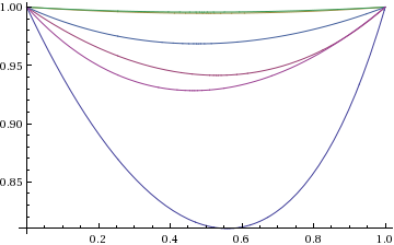
(a) Momentum variance $\sigma_{p;t}^{2}$

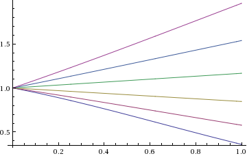
(b) Position variance $\sigma_{q;t}^{2}$ for $\partial_{q}\partial_{p}S=0$

(c) Contribution to the entropy production by a change of position variance

Figure 1: Evolution of the fluctuation variances for $t_{\mathrm{f}}=1$ and $\tau=0.1$. As in subsection 7.2.3 we assume $\sigma_{p;\mathrm{o}}=\sigma_{p;\mathrm{f}}=\sigma_{q;\mathrm{o}}=1$ and $\theta_{\mathrm{f}}=0$. Correspondingly, we plot fig. 1(b) after imposing $\partial_{q}\partial_{p}S=0$ in the control horizon. The plots correspond to different values of $\delta=\sigma_{q;\mathrm{f}}-1$. In fig 1(a) the constant value of $\sigma_{p;t}$ corresponds to $\sigma_{q;\mathrm{f}}=1.0$. The larger the absolute value of the deviation from unity of $\sigma_{q;\mathrm{f}}$, the larger the departure of $\sigma_{p;t}$ from the unity inside the control horizon. In fig 1(c) we plot the corresponding values of $\mathcal{E}_{t_{\mathrm{f}},0}-\beta\mu_{q;\mathrm{f}}^{2}\tau/t_{\mathrm{f}}$

In fig. 1 we report the behavior of the momentum and position variance for vanishing cross-correlation. It is worth emphasizing that the momentum variance does not remain constant during the control horizon unless

$$\sigma_{q;\mathrm{f}}=\sigma_{q;\mathrm{o}}=\Omega=0$$ (91)

7.2.3 “Over-damped” limit: $\theta_{\mathrm{f}}=\sigma_{p;\mathrm{f}}-\sigma_{p;\mathrm{o}}=0$ and $\varepsilon=(\sigma_{q;\mathrm{f}}-\sigma_{q;\mathrm{o}})/\sigma_{q;\mathrm{o}}$ for $\lambda\,\ll\,1$

At variance with the foregoing  we now assume a wide scale separation between the position and momentum variance. We readily see from (86) that $(\varphi\,,\Omega)=(-\pi+O(\lambda)\,,O(\lambda))$. We can solve the boundary condition equations (74) in the limit of vanishing $\lambda$ up to all order accuracy in $\varepsilon$:

$$\Omega=\frac{2\,\lambda\,\varepsilon}{t_{\mathrm{f}}}\left\{1-\varepsilon+\frac{2\,\varepsilon^{2}}{3}+O(\varepsilon^{3})\right\}\overset{\lambda\downarrow 0}{\to}\frac{6\,\lambda\,\varepsilon}{t_{\mathrm{f}}\,\left[3+\varepsilon\,(3+\varepsilon)\right]}+o(\lambda)$$ (92a)

$$\varphi=-\pi+2\,\lambda\left\{1-\varepsilon+\frac{2\,\varepsilon^{2}}{3}+O(\varepsilon^{3})\right\}\overset{\lambda\downarrow 0}{\to}-\pi+\frac{\Omega\,t_{\mathrm{f}}}{\varepsilon}+o(\lambda)$$ (92b)

The corresponding value of the entropy production is

$$\frac{\mathcal{E}_{t_{\mathrm{f}},0}}{\beta}=\frac{\mu_{q;\mathrm{f}}^{2}\,\tau}{t_{\mathrm{f}}}+\frac{(\sigma_{q;\mathrm{f}}-\sigma_{q;\mathrm{o}})^{2}}{\beta\,t_{\mathrm{f}}}+o\left(\lambda\right)$$ (93)

We notice that this is exactly the entropy production by a transition governed by a Langevin–Smoluchowski dynamics between Gaussian states [9, 7, 16]. Indeed, the regime we are considering here corresponds to the “over-damped” asymptotics of the Langevin–Kramers dynamics. Namely, upon inserting (92) into the quadratic Ansätze for the non-equilibrium Helmholtz energy and microscopic entropy densities we get into

$$\left.(\partial_{q}A)(0,q,t)\right|_{\mu_{p;t}=0}=-\frac{\mu_{q;\mathrm{f}}\,+\frac{q\,(\sigma_{q;\mathrm{f}}-\sigma_{q;\mathrm{o}})}{\sigma_{q;\mathrm{o}}}}{1+\frac{t\,\left(\sigma_{q;\mathrm{f}}-\sigma_{q;\mathrm{o}}\right)}{t_{\mathrm{f}}\,\sigma_{q;\mathrm{o}}}}\frac{\tau}{t_{\mathrm{f}}}+o\left(\lambda\right)$$ (94a)

$$\left.(\partial_{p}A)(0,q,t)\right|_{\mu_{p;t}=0}=-\left.(\partial_{p}A)(0,q,t)\right|_{\mu_{p;t}=0}+o\left(\lambda\right)$$ (94b)

$$(\partial_{q}S)(0,q,t)=\frac{\beta\,\left(q-\frac{\mu_{q;\mathrm{f}}\,t}{t_{\mathrm{f}}}\right)}{\sigma_{q;\mathrm{o}}^{2}\,\left[1+\frac{t\,(\sigma_{q;\mathrm{f}}-\sigma_{q;\mathrm{o}})}{t_{\mathrm{f}}\,\sigma_{q;\mathrm{o}}}\right]^{2}}+o(\lambda)$$ (94c)

We see that the $\lambda$-independent parts of (94a) and (94c) coincide with the values obtained for the same quantities in the Langevin–Smoluchowski case [9, 7, 16]. In the forthcoming section, we will show that (54) encapsulate also in general the results obtained for Langevin–Smoluchowski dynamics. In particular, the equality (94b) guarantees that an homogenization theory “centering condition” holds for the Gaussian model so that the Langevin–Smoluchowski dynamics is recovered as the solution of a suitable “cell problem” [25].

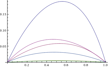
(a) Relative variation of the momentum variance for $\sigma_{p;\mathrm{o}}=\lambda=1$

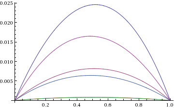
(b) Relative variation of the momentum variance for $\sigma_{p;\mathrm{o}}=\lambda=0.1$

Figure 2: Relative variation $|\sigma_{p;t}^{2}-\sigma_{p;\mathrm{o}}^{2}|/\sigma_{p;\mathrm{o}}^{2}$ for $\sigma_{p;\mathrm{o}}=1$ fig. 2(a) and $\sigma_{p;\mathrm{o}}=0.1$ fig. 2(a). In both cases $\sigma_{q;\mathrm{o}}=1$ so that $\sigma_{p;\mathrm{o}}=\lambda$. The other parameters as in fig. 2. As $\lambda$ decreases, the approximation of the marginal momentum distribution by an “equilibrium” distribution improves its accuracy while remaining not uniform inasmuch the deviation increases with $(\sigma_{q;\mathrm{f}}-\sigma_{q;\mathrm{o}})^{2}$ and reaches a maximum for $t\sim t_{\mathrm{f}}/2$.

8 “Over-damped” asymptotics

In the presence of a wide separation of between the characteristic scales of the momentum and position variables, the Langevin–Smoluchowski or “over-damped” dynamics often provides a good approximation to the Langevin–Kramers dynamics. The entropy production by a smooth Langevin–Smoluchowski dynamics attains a minimum value if the control potential obeys a Monge–Ampère–Kantorovich dynamics [8, 9, 7, 16]. In this last section our aim is to investigate in which sense we can recover from (54) the results previously established for Langevin-Smoluchowski dynamics. To address this question, we suppose that the probability densities of the initial and final states take the additive form

$$\mathtt{m}_{\mathrm{o}}(\bm{p},\bm{q})=\left(\frac{\beta}{2\,\pi\,\lambda}\right)^{d}\exp\left\{-\beta\,\frac{\parallel\bm{p}\parallel_{\mathsf{1}_{d}}^{2}}{2\,\lambda^{2}}-\beta\,U_{\mathrm{o}}(\bm{q})\right\}$$ (95)

and

$$\mathtt{m}_{\mathrm{f}}(\bm{p},\bm{q})=\left(\frac{\beta}{2\,\pi\,\lambda}\right)^{d}\exp\left\{-\beta\,\frac{\parallel\bm{p}\parallel_{\mathsf{1}_{d}}^{2}}{2\,\lambda^{2}}-\beta\,U_{\mathrm{f}}(\bm{q})\right\}$$ (96)

with $\lambda\,\ll\,1$ a non-dimensional parameter generalizing (88) in order to describe the scale separation between momentum and position dynamics.

Multi-scale perturbation theory (often also referred to as homogenization theory see e.g. [24, 25]) in powers of $\lambda$ equips us with the tools to extricate the asymptotic expression of solutions of (54) for $\beta\,\parallel\bm{p}\parallel_{\mathsf{1}_{d}}^{2}\ll\lambda\ll\,1$ in the form

$$A(\bm{x},t)=\sum_{i=0}^{2}\,\lambda^{i}\,A_{(i)}\left(\frac{\bm{p}}{\lambda},\bm{q},t\dots\right)+o(\lambda^{2}):=\tilde{A}\left(\tilde{\bm{p}},\bm{q},t\dots\right)$$ (97)

and similarly for $S$ and $V$. The $\dots$ in (97) portend the scales which we eventually neglect in the asymptotics. Once we availed us of (97), the extremal equations (54) become

$$\frac{1}{\lambda}\bm{\left(}\tilde{S}\,,\tilde{V}\bm{}_{\mathsf{J}^{\dagger}}^{\sim}+\frac{1}{\lambda^{2}\,\beta}\tilde{\mathfrak{S}}(\tilde{V}-2\,\tilde{A})=0$$ (98a)

$$\tau\,\partial_{t}\tilde{V}+\frac{1}{\lambda}\bm{\left(}\tilde{A}\,,\tilde{V}\bm{}_{\mathsf{J}^{\dagger}}^{\sim}-\frac{1}{\lambda^{2}}\left(\partial_{\tilde{\bm{p}}}\tilde{A}\right)\overset{d}{\cdot}\partial_{\tilde{\bm{p}}}\left(\tilde{V}-\tilde{A}\right)=0$$ (98b)

$$\tau\,\partial_{t}\tilde{S}+\frac{1}{\lambda}\bm{\left(}\tilde{A}\,,\tilde{S}\bm{}_{\mathsf{J}^{\dagger}}^{\sim}+\frac{1}{\lambda^{2}\,\beta}\tilde{\mathfrak{S}}\tilde{A}=0$$ (98c)

where we used the notation $\tilde{\bm{x}}=\bm{q}\oplus\bm{\tilde{p}}$

$$\bm{\left(}\tilde{S}\,,\tilde{V}\bm{}_{\mathsf{J}^{\dagger}}^{\sim}\equiv(\partial_{\bm{\tilde{x}}}\tilde{S})\cdot\left(\mathsf{J}^{\dagger}\cdot\partial_{\bm{\tilde{x}}}\tilde{V}\right)=(\partial_{\tilde{\bm{p}}}\tilde{S})\overset{d}{\cdot}\partial_{\bm{q}}\tilde{V}-(\partial_{\bm{q}}\tilde{S})\overset{d}{\cdot}\partial_{\tilde{\bm{p}}}\tilde{V}$$ (99)

and

$$\tilde{\mathfrak{S}}:=-(\partial_{\tilde{\bm{p}}}\tilde{S})\overset{d}{\cdot}\partial_{\tilde{\bm{p}}}+\mathsf{1}_{d}:\partial_{\tilde{\bm{p}}}\otimes\partial_{\tilde{\bm{p}}}$$ (100)

In what follows, we will also write $\tilde{\mathfrak{S}}^{(0)}$ to denote the replacement in (100) of $\tilde{S}$ with its zeroth order approximation $\tilde{S}^{(0)}$.

As often occurs for homogenization of parabolic equation [25], we need to analyze the first three orders of the regular expansion in powers of $\lambda$ in order to fully determine the leading order contributions to $S$ and $A$. This is because the first order is needed to assess the centering condition coupling the widely separated scales which we wish to resolve in the asymptotics. The second order approximation uses the information conveyed by the centering condition to determine the cell problem, a closed equation for the effective dynamics in the limit of vanishing $\lambda$.

8.1 Zeroth order

From (98a) we get the condition

$$\tilde{\mathfrak{S}}^{(0)}\left(2\,A_{(0)}-V_{(0)}\right)=0$$ (101)

stating that at leading order the value function $V_{(0)}$ may differ from the non equilibrium Helmholtz energy at most by a function independent of momentum variables:

$$V_{(0)}=2\,A_{(0)}+V_{(0:0)}$$ (102)

where

$$\partial_{\tilde{\bm{p}}}V_{(0:0)}=0$$ (103)

Once we inserted (102) in (98b), (98c) we get into

$$\partial_{\tilde{\bm{p}}}A_{(0)}\overset{d}{\cdot}\partial_{\tilde{\bm{p}}}A_{(0)}=0$$ (104a)

$$\frac{1}{\beta}\tilde{\mathfrak{S}}^{(0)}A_{(0)}=0$$ (104b)

The boundary conditions (95), (96) translate into

$$S_{\mathrm{o}}=S_{\mathrm{f}}+o(\lambda^{2})$$ (105)

Hence, we see from (104) that (105) is satisfied upon setting

$$S_{(0)}(\tilde{\bm{p}})=\frac{\parallel\tilde{\bm{p}}\parallel_{\mathsf{1}_{d}}^{2}}{2}+S_{(0:0)}(\bm{q},t,\dots)$$ (106)

and

$$\partial_{\tilde{\bm{p}}}A_{(0)}=\partial_{\tilde{\bm{p}}}V_{(0)}=0$$ (107)

8.2 First order: centering condition

Maxwell momentum distribution is the unique element of the kernel of $\tilde{\mathfrak{S}}^{(0)\dagger}$ in $\mathbb{L}^{2}(\mathbb{R}^{d})$. By Fredholm alternative (see e.g. [25])

$$\bm{\left(}S_{(0)}\,,V_{(0)}\bm{}_{\mathsf{J}^{\dagger}}^{\sim}-\frac{1}{\beta}\tilde{\mathfrak{S}}^{(0)}(2\,A_{(1)}-V_{(1)})=0$$ (108)

admits a unique solution if and only if the solvability condition

$$0=\int_{\mathbb{R}^{d}}\mathrm{d}^{d}p\,e^{-S_{(0)}}\bm{\left(}S_{(0)}\,,V_{(0)}\bm{}_{\mathsf{J}^{\dagger}}^{\sim}=$$ (109)

$$-\int_{\mathbb{R}^{d}}\mathrm{d}^{d}p\,\bm{\left(}e^{-S_{(0)}}\,,V_{(0)}\bm{}_{\mathsf{J}^{\dagger}}^{\sim}=\partial_{\bm{q}}\int_{\mathbb{R}^{d}}\mathrm{d}^{d}p\,e^{-S_{(0)}}\partial_{\tilde{\bm{p}}}V_{(0)}$$

holds true which is always the case if (107) is verified. Hence we conclude

$$V_{(1)}=2\,\left(A_{(1)}+\tilde{\bm{p}}\cdot\partial_{\bm{q}}A_{(0)}\right)+\tilde{\bm{p}}\cdot\partial_{\bm{q}}V_{(0:0)}+V_{(1:0)}$$ (110)

with

$$\partial_{\tilde{\bm{p}}}V_{(1:0)}=0$$ (111)

Turning to the value function equation (98b), we see that

$$-\sum_{i=0}^{1}\partial_{\tilde{\bm{p}}}V_{(1-i)}\overset{d}{\cdot}\partial_{\tilde{\bm{p}}}A_{(i)}+\bm{\left(}A_{(0)}\,,V_{(0)}\bm{}_{\mathsf{J}^{\dagger}}^{\sim}+2\,\partial_{\tilde{\bm{p}}}A_{(1)}\overset{d}{\cdot}\partial_{\tilde{\bm{p}}}A_{(0)}=0$$ (112)

is also satisfied by (107). New information comes from the expansion of the microscopic entropy equation

$$-\partial_{\bm{q}}A_{(0)}\cdot\partial_{\tilde{\bm{p}}}S_{(0)}+\tilde{\mathfrak{S}}^{(0)}A_{(1)}=0$$ (113)

which yields the centering condition of the expansion:

$$A_{(1)}=-\tilde{\bm{p}}\cdot\partial_{\bm{q}}A_{(0)}$$ (114)

The centering condition couples here a linear asymptotic behavior in $\bm{p}$ with a non-trivial cell problem in $(\bm{q},t)$ which we will determine by requiring solvability in the sense of Fredholm’s alternative at order $O(\lambda^{2})$. Contrasting (114) with (110) we infer that

$$\partial_{\tilde{\bm{p}}}V_{(1)}=\partial_{\bm{q}}V_{(0:0)}$$ (115)

It is worth here to emphasize the relevant simplification induced by the over-damped limit. The over-damped limit entitled us to neglect the Poisson bracket also in the sub-leading order (108) of the expansion of (54c). The crucial consequence is that the relation between $V$ and $A$ remains local within accuracy. Intermediate asymptotics around (104) do not enjoy this property. This is not surprising in light of example of section 7.2.3 showing that, even in the Gaussian case, the coincidence of the initial and final marginal momentum distribution does not imply in general thermalization.

8.3 Second order: cell problem

The extremal equation (98a) yields now the condition

$$\partial_{\tilde{\bm{p}}}S_{(0)}\overset{d}{\cdot}\partial_{\bm{q}}V_{(1)}-\partial_{\bm{q}}S_{(0)}\overset{d}{\cdot}\partial_{\bm{q}}V_{(0,0)}-\frac{1}{\beta}\tilde{\mathfrak{S}}^{(0)}(2\,A_{(2)}-V_{(2)})=0$$ (116)

The solvability condition imposes

$$\partial_{\bm{q}}V_{(0,0)}=0$$ (117)

whence

$$V_{(2)}=2\,A_{(2)}+\tilde{\bm{p}}\cdot\partial_{\bm{q}}V_{(1:0)}+V_{(2:0)}$$ (118)

with $\partial_{\tilde{\bm{p}}}V_{(2:0)}=0$. Hence, combining (102) with (117), (114) and (105), the value function equation reduces to

$$2\,\tau\,\partial_{t}A_{(0)}-\partial_{\bm{q}}A_{(0)}\overset{d}{\cdot}\partial_{\bm{q}}A_{(0)}=0$$ (119)

Finally, the equation for the microscopic entropy is

$$\partial_{t}S_{(0)}-\partial_{\bm{q}}A_{(0)}\overset{d}{\cdot}\partial_{\bm{q}}S_{(0)}+\tilde{\bm{p}}\cdot\partial_{\bm{q}}\otimes\partial_{\bm{q}}A_{(0)}\cdot\partial_{\tilde{\bm{p}}}S_{(0)}+\frac{1}{\beta}\tilde{\mathfrak{S}}^{(0)}A_{(2)}=0$$ (120)

Regarding this latter as an equation for $A_{(2)}$ and invoking again Fredholm’s alternative, we see that it admits a unique solution if and only if

$$\tau\,\partial_{t}S_{(0:0)}-\partial_{\bm{q}}A_{(0)}\overset{d}{\cdot}\partial_{\bm{q}}S_{(0:0)}+\frac{1}{\beta}\mathsf{1}_{d}:\partial_{\bm{q}}\otimes\partial_{\bm{q}}A_{(0)}=0$$ (121)

holds true. The system formed by the equalities (106), (114) and the cell problem equations (119), (121) fully specifies the homogenization asymptotics we set out to derive.

8.4 Asymptotic expression of the entropy production

The cell problem equations (119), (121) specify a Monge–Ampère–Kantorovich evolution [26] between a initial configuration space state with density

$$\tilde{\mathtt{m}}_{\mathrm{o}}(\bm{q})=\left(\frac{\beta}{2\,\pi}\right)^{d/2}\,e^{-\beta\,U_{\mathrm{o}}(\bm{q})}$$ (122)

and a final one with density

$$\tilde{\mathtt{m}}_{\mathrm{f}}(\bm{q})=\left(\frac{\beta}{2\,\pi}\right)^{d/2}\,\,e^{-\beta\,U_{\mathrm{f}}(\bm{q})}$$ (123)

The recovery of the Monge–Ampère–Kantorovich equations unveils the link between the minimum entropy production by the phase space process (1) and the optimal control of the corresponding thermodynamic quantity which can be directly defined in the over-damped limit. As a matter of fact, the expansion of $A$ starts with the $O(\lambda)$ term specified by the centering condition (114) which is linear in $\tilde{\bm{p}}=\bm{p}/\lambda$. The upshot is that the over-damped expansion of the minimum over $\mathbb{A}$ of the Langevin–Kramers entropy production starts with

$$\mathcal{E}_{t_{\mathrm{f}},0}=\beta\,\int_{0}^{t_{\mathrm{f}}}\frac{\mathrm{d}t}{\tau}\int_{\mathbb{R}^{d}}\mathrm{d}^{d}q\,\beta^{d/2}e^{-S_{(0,0)}}\left(\partial_{\bm{q}}A_{(0)}\right)\overset{d}{\cdot}\partial_{\bm{q}}A_{(0)}+O(\lambda)$$ (124)

We therefore proved that the leading order of the expansion coincides with the minimal entropy production by the Langevin–Smoluchowski dynamics.

9 Discussion

Many physical systems are modeled by kinetic-plus-potential Hamiltonians

$$H(\bm{p},\bm{q})=\frac{\parallel\bm{p}\parallel_{\mathsf{1}_{d}}^{2}}{2}+U(\bm{q},t)$$ (125)

The example of section 7.1 evinces that requiring (125) adds an optimization constraint which is not generically satisfied by the extremal equations (54) over $\mathbb{A}$. Furthermore, the kinetic-plus-potential hypothesis deeply affects the control problem by introducing two new difficulties. First, it restricts to the gradient $\partial_{\bm{q}}U$ of the potential energy the available $d$ control degrees of freedom. In this regard, it is worth emphasizing that it is a non-trivial consequence of Hörmander theorem (see e.g. [27] and references therein) that a sufficiently regular (125) is enough to generate a Fokker–Planck evolution of a smooth initial density for a Langevin–Kramers dynamics with degenerate noise acting only on $d$ out of $2\,d$ degrees of freedom. Physical intuition suggests, however, that the surmise (125) should not create an insurmountable difficulty for controllability by which we mean the existence of a non-empty set of potentials $U(\bm{q},t)$ able to steer a transition between two probability densities verifying physically plausible assumptions. The second and more substantial difficulty is that inserting (125) into (25) yields an entropy production expression which depends upon the control only implicitly through the probability measure. Controls are in such a case only subject to the constraint imposed by the requirement of steering a finite-time transition between smooth probability densities. General considerations [17] lead us to envisage that entropy production may only attain an infimum when evaluated according to a singular control strategy. Such a strategy may take the form of a potential $U$ confining the momentum process within a “inactivity region” where $U$ vanishes. We expect the boundary of such inactivity region to be marked by the the vanishing of the momentum gradient $\partial_{\bm{p}}V$ of the value function of the corresponding dynamic programming equation. Proving the realizability and optimality of such a control strategy are challenges lying beyond the scopes of the present work. By insisting that the Hamiltonian belongs to the class of admissible controls $\mathbb{A}$, we focused instead on control strategies which we interpret as “macroscopic” in view the regularity assumptions on the control Hamiltonian. These assumptions are analogous to those adopted in previous studies of the entropy production by Langevin–Smoluchowski dynamics [7] or by Markov jump processes [11]. We therefore gather that the existence of the entropy production minimum (54), degenerate because of non-coercivity, and which recovers in the over-damped limit the Monge–Ampère–Kantorovich evolution, yields a robust general picture of the “optimal” thermodynamics for a large class of physical processes described by Markovian evolution equations.

Appendices

Appendix A Mean derivatives and current velocity of a diffusion process

We recall that the drift of an $\mathbb{R}^{d}$-valued diffusion processes $\zeta\equiv\left\{\bm{\zeta}_{t}\,,\hskip 2.84544ptt\in\,[t_{\mathrm{o}}\,,t_{\mathrm{f}}]\right\}$ with generator

$$\mathfrak{L}=\bm{b}\cdot\partial_{\bm{x}}+\frac{1}{2}\mathsf{K}:\partial_{\bm{x}}\otimes\partial_{\bm{x}}$$ (126)

can be regarded as the mean forward derivative of the process:

$$\mathrm{D}_{\bm{x}}\bm{\zeta}_{t}\equiv\lim_{\mathrm{d}t\downarrow\,0}\mathrm{E}_{\bm{\zeta}_{t}=\bm{x}}\frac{\bm{\zeta}_{t+\mathrm{d}t}-\bm{\zeta}_{t}}{\mathrm{d}t}=\mathfrak{L}\,\bm{x}$$ (127)

Under standard regularity hypotheses [32], it is possible to define the mean backward derivative of the very same process as

$$\mathrm{D}_{\bm{x}}^{-}\bm{\zeta}_{t}\equiv\lim_{\mathrm{d}t\downarrow\,0}\mathrm{E}_{\bm{\zeta}_{t}=\bm{x}}\frac{\bm{\zeta}_{t}-\bm{\zeta}_{t-\mathrm{\mathrm{d}t}}}{\mathrm{d}t}$$ (128)

Proposition A.1.

Let $\zeta\equiv\left\{\bm{\zeta}_{t}\,,\hskip 2.84544ptt\in\,[t_{\mathrm{o}}\,,t_{\mathrm{f}}]\right\}$ be a smooth diffusion with generator (126) and density $\mathtt{m}$. The mean forward derivative is

$$\mathrm{D}_{\bm{x}}^{-}\bm{\zeta}_{t}=-\frac{1}{\mathtt{m}(\bm{x},t)}\frac{\left(\mathfrak{L}^{\dagger}\,\bm{x}-\bm{x}\,\mathfrak{L}^{\dagger}\,\right)}{\tau}\mathtt{m}(\bm{x},t)$$ (129)

Proof.

By hypothesis $\zeta$ is Markovian with density $\mathtt{m}$ in the time interval $[t_{\mathrm{o}},t_{\mathrm{f}}]$. Given its forward transition probability density $\mathtt{p}$ the backward transition probability $\mathtt{p}_{*}$ of the same process density must then satisfy

$$\mathtt{p}_{*}(\bm{x}_{1},t_{1}|\bm{x}_{2},t_{2})=\frac{1}{\mathtt{m}(\bm{x}_{2},t_{2})}\mathtt{p}(\bm{x}_{2},t_{2}|\bm{x}_{1},t_{1})\,\mathtt{m}(\bm{x}_{1},t_{1})$$ (130)

for any $\bm{x}_{1},\bm{x}_{2}\in\mathbb{R}^{d}$, $t_{1},t_{2}\in[t_{\mathrm{o}},t_{\mathrm{f}}]$ such that $t_{2}\geq t_{1}$. By (130) it follows immediately

$$\mathrm{E}_{\bm{\zeta}_{t}=\bm{x}}\bm{\zeta}_{t-\mathrm{d}t}=\int\mathrm{d}^{2d}x_{1}\,\bm{x}_{1}\,\frac{\mathtt{p}(\bm{x},t|\bm{x}_{1},t-\mathrm{d}t)\,\mathtt{m}(\bm{x}_{1},t-\mathrm{d}t)}{\mathtt{m}(\bm{x},t)}$$ (131)

If we integrate the Fokker-Planck and its adjoint equation over a time horizon of order $O(\mathrm{d}t)$ we arrive at

$$\mathrm{E}_{\bm{\zeta}_{t}=\bm{x}}\bm{\zeta}_{t-\mathrm{d}t}=\bm{x}+$$ (132)

$$\frac{\mathrm{d}t}{\tau}\int\mathrm{d}^{2d}x_{1}\,\bm{x}_{1}\,\frac{\mathtt{m}(\bm{x}_{1},t)\,\mathfrak{L}\,\delta^{(2d)}(\bm{x}_{1}-\bm{x})-\delta^{(2d)}(\bm{x}_{1}-\bm{x})\,\mathfrak{L}^{\dagger}\,\mathtt{m}(\bm{x}_{1},t)}{\mathtt{m}(\bm{x},t)}+O\left(\frac{\mathrm{d}t}{\tau}\right)$$

which inserted in the definition (128) yields the claim. ∎

The mean backward drift governs the Fokker-Planck evolution of the density of the process from $t_{\mathrm{f}}$ to $t_{\mathrm{o}}$ [32]. By Hörmander theorem [27], the proposition above encompasses the degenerate noise case described by (1). We are therefore entitled to write

$$\tau\,\mathrm{D}_{\bm{x}}^{-}\bm{\chi}_{t}=\mathsf{J}\cdot\partial_{\bm{x}}H-\mathsf{G}\cdot\partial_{\bm{x}}\left(H+\frac{2}{\beta}\ln\frac{\mathtt{m}}{\beta^{d}}\right)$$ (133)

The current velocity of a smooth diffusion is defined as

$$\bm{v}(\bm{x},t)\equiv\,\tau\,\frac{D_{\bm{x}}+D_{\bm{x}}^{-}}{2}\bm{\zeta}_{t}$$ (134)

whence (24) follows immediately. The advantage of the current velocity representation is that the Fokker-Planck equation for the probability density $\mathtt{m}$ in $[t_{\mathrm{o}}\,,t_{\mathrm{f}}]$ is mapped by (134) into the deterministic mass conservation equation

$$\tau\,\partial_{t}\mathtt{m}+\partial_{\bm{x}}\cdot\bm{v}\,\mathtt{m}=0$$ (135)

Appendix B Variations of the Pontryagin functional

We avail us of the identity (52) to treat (49) as a functional of the independent fields $A$ and $\mathtt{m}$. The variation of (49) with respect to the costate function being trivial, we restrict here the attention only to those with respect to the probability density $\mathtt{m}$ and the non-equilibrium Helmholtz energy density $A$. The boundary terms generated by the variation of $\mathtt{m}$ vanish because of the boundary conditions (50):

$$\mathcal{A}_{\mathtt{m}}^{\prime}(\mathtt{m},V,A)=$$ (136)

$$\int_{t_{\mathrm{o}}}^{t_{\mathrm{f}}}\frac{\mathrm{d}t}{\tau}\,\int_{\mathbb{R}^{2\,d}}\mathrm{d}^{2\,d}x\,\mathtt{m}^{\prime}\left\{\parallel\partial_{\bm{x}}A\parallel_{\mathsf{G}}^{2}+[\tau\,\partial_{t}+(\partial_{\bm{x}}A)\cdot(\mathsf{J}^{\dagger}-\mathsf{G})\cdot\partial_{\bm{x}}]V\right\}$$

Upon applying the definition of the brackets (14), (15) we arrive at (54a). The variation of $A$ can be couched into the form

$$\mathcal{A}_{A}^{\prime}(\mathtt{m},V,A)=-\int_{t_{\mathrm{o}}}^{t_{\mathrm{f}}}\frac{\mathrm{d}t}{\tau}\,\int_{\mathbb{R}^{2\,d}}\mathrm{d}^{2\,d}x\,A^{\prime}\partial_{\bm{x}}\cdot\mathtt{m}\,\left\{2\,\mathsf{G}\cdot\partial_{\bm{x}}A-(\mathsf{J}^{\dagger}-\mathsf{G})\cdot\partial_{\bm{x}}V\right\}$$ (137)

Recalling the definition of the microscopic entropy (7), we see that stationarity of (137) admits a geometric interpretation on the De Rahm–Witten complex over $\mathbb{L}^{(2)}(\mathbb{R}^{2d},\mathtt{m}\,\mathrm{d}^{2d}x)$ [48] equipped with the exterior derivative

$$\mathrm{d}_{S}=e^{-S}\mathrm{d}\,e^{S}$$ (138)

Namely it states that the dual $\mathrm{d}_{S}^{*}$ to (138) must annihilate the $\mathrm{1}$-form

$$\mathsf{\alpha}=[2\,\partial_{\bm{x}}A+(\mathsf{J}+\mathsf{G})\cdot\partial_{\bm{x}}V]\cdot\mathrm{d}x$$ (139)

In terms of the operator (55) the condition translates into (54c). We also notice that that (55) is a degenerate “Witten” Laplacian [48] on the same complex in consequence of the inequality

$$\int_{\mathbb{R}^{2d}}\mathrm{d}^{2d}x\,\mathtt{m}\,f\,\mathfrak{S}\,f=-\int_{\mathbb{R}^{2d}}\mathrm{d}^{2d}x\,\mathtt{m}\,\parallel\partial_{\bm{x}}f\parallel_{\mathsf{G}}^{2}\,\leq\,0$$ (140)

holding for any $f\,\in\,\mathbb{L}^{2}(\mathbb{R}^{2d},\mathtt{m}\,\mathrm{d}^{2d}x)$.

We end this this appendix with a remark. If the nullspace in $\mathbb{L}^{(2)}(\mathbb{R}^{2d},\mathtt{m}\,\mathrm{d}^{2d}x)$ of the Witten Laplacian

$$\bar{\mathfrak{S}}=-(\partial_{\bm{x}}S)\cdot\partial_{\bm{x}}+\mathsf{1}_{2d}:\partial_{\bm{x}}\otimes\partial_{\bm{x}}$$ (141)

consists only of constant functions then on the De Rahm–Witten complex (138) then current velocity (24) admits the Hodge decomposition

$$\bm{v}=-\partial_{\bm{x}}H_{0}+\bm{h}_{2}$$ (142)

where $H_{0}$ is a differentiable phase-space function specified by the solution of

$$\bar{\mathfrak{S}}\,H_{0}=-\bm{\left(}S\,,A\bm{}_{\mathsf{J}^{\dagger}}+\mathfrak{S}A$$ (143)

and

$$\bm{h}_{2}\equiv\,e^{S}\partial_{\bm{x}}\cdot\,e^{-S}\mathsf{H}_{2}$$ (144)

$\mathsf{H}_{2}$ being differentiable anti-symmetric rank-two tensor. By construction the elements of the decomposition in (142) are orthogonal in $\mathbb{L}^{(2)}(\mathbb{R}^{2d},\mathtt{m}\,\mathrm{d}^{2d}x)$.

There are two interesting consequences of (142). The first is that mass-transport equation for $\mathtt{m}$ depends only upon $H_{0}$ owing to

$$\partial_{\bm{x}}\cdot\left(\mathtt{m}\,e^{S}\partial_{\bm{x}}\cdot\,e^{-S}\mathsf{H}_{2}\right)=\beta^{d}\partial_{\bm{x}}\otimes\partial_{\bm{x}}:e^{-S}\mathsf{H}_{2}=0$$ (145)

The second is that identifying the the gradient in (142) as the dissipative component of the dynamics allows us to define the “entropy production”

$$\tilde{\mathcal{E}}_{t_{\mathrm{f}},t_{\mathrm{o}}}=\beta\,\int_{t_{\mathrm{o}}}^{t_{\mathrm{f}}}\frac{\mathrm{d}t}{\tau}\int_{\mathbb{R}^{2d}}\mathrm{d}^{2d}x\,\mathtt{m}\,\parallel\partial_{\bm{x}}H_{0}\parallel^{2}$$ (146)

At variance with (25), is a coercive functional of $H_{0}$ the optimal control whereof reduces by (145) to that of the Langevin–Smoluchowski case in $\mathbb{R}^{2d}$. It must be stressed, however, that carries different physical information than (25) since this latter depends also on $\bm{h}_{2}$.

References

References

- [1] Ritort F 2008 Nonequilibrium Fluctuations in Small Systems: From Physics to Biology Advances in Chemical Physics vol 137 ed Rice S A (John Wiley & Sons, Inc., Hoboken, NJ, USA.) (Preprint 0705.0455)
- [2] Haynie D T 2008 Biological thermodynamics 2nd ed (Cambridge University Press) ISBN -13: 978-0-521-71134-0; e-ISBN-13: 978-0-511-38637-4
- [3] Savir Y and Tlusty T 2013 Cell 153 471 – 479 ISSN 0092-8674 URL http://www.weizmann.ac.il/complex/tlusty/research.html
- [4] Bennett C H 1982 International Journal of Theoretical Physics 21 905–940
- [5] Landauer R 1961 IBM Journal of Research and Development 5 183–191 URL http://researchweb.watson.ibm.com/journal/rd/053/ibmrd0503C.pdf
- [6] Bérut A, Arakelyan A, Petrosyan A, Ciliberto S, Dillenschneider R and Lutz E 2012 Nature 483 187–189
- [7] Aurell E, Gawȩdzki K, Mejía-Monasterio C, Mohayaee R and Muratore-Ginanneschi P 2012 Journal of Statistical Physics 147 487–505 (Preprint 1201.3207)
- [8] Aurell E, Mejía-Monasterio C and Muratore-Ginanneschi P 2011 Physical Review Letters 106 250601 (Preprint 1012.2037)
- [9] Aurell E, Mejía-Monasterio C and Muratore-Ginanneschi P 2012 Physical Review E 85(2) 020103(R) (Preprint 1111.2876) URL http://link.aps.org/doi/10.1103/PhysRevE.85.020103
- [10] Gawȩdzki K 2013 Fluctuation Relations in Stochastic Thermodynamics lecture notes (Preprint 1308.1518)
- [11] Muratore-Ginanneschi P, Mejía-Monasterio C and Peliti L 2013 Journal of Statistical Physics 150 181–203 (Preprint 1203.4062)
- [12] Alemany A, Ribezzi M and Ritort F 2011 AIP Conference Proceedings 1332 96–110 (Preprint 1101.3174) URL http://link.aip.org/link/?APC/1332/96/1
- [13] Sekimoto K 1998 Progress of Theoretical Physics Supplement 130 17–27
- [14] Sekimoto K 2010 Stochastic Energetics (Lecture Notes in Physics vol 799) (Springer) ISBN -13: 978-3-642-05410-5
- [15] Jiang D Q, Qian M and Qian M P 2004 Mathematical Theory of Nonequilibrium Steady States (Lecture Notes in Mathematics vol 1833) (Springer) ISBN -13: 978-3-540-20611-8
- [16] Muratore-Ginanneschi P 2013 Journal of Physics A: Mathematical and General 46 275002 (Preprint 1210.1133)
- [17] Fleming W H and Soner M H 2006 Controlled Markov processes and viscosity solutions 2nd ed (Stochastic modelling and applied probability vol 25) (Springer) ISBN -13: 978-0-387-26045-7
- [18] Kullback S and Leibler R 1951 Annals of Mathematical Statistics 22 79–86 URL http://projecteuclid.org/euclid.aoms/1177729694
- [19] Fleming W and Rishel R 1975 Deterministic and Stochastic Optimal Control Applications of Mathematics (Springer) ISBN -13: 978-1-461-26382-1; e-ISBN-13: 978-1-461-26380-7
- [20] Malliaris A G and Brock W A 1999 Stochastic methods in economics and finance 8th ed (Advanced textbooks in economics vol 17) (Elsevier Science) ISBN -13: 978-0-444-86201-3
- [21] Evans L C An Introduction to Mathematical Optimal Control Theory lecture notes, University of California at Berkeley URL http://math.berkeley.edu/~evans/control.course.pdf
- [22] Guerra F and Morato L M 1983 Physical Review D 27 1774–1786
- [23] van Handel R 2007 Stochastic Calculus and Stochastic Control lecture notes, Caltech URL http://www.princeton.edu/~rvan/acm217/ACM217.pdf
- [24] Bensoussan A, Lions J L and Papanicolaou G 1978 Asymptotic Analysis for Periodic Structures (Studies in mathematics and its applications vol 5) (North-Holland, Amsterdam) ISBN -13: 978-0-444-85172-7
- [25] Pavliotis G A and Stuart A M 2008 Multiscale methods: averaging and homogenization (Texts in applied mathematics vol 53) (Springer) ISBN -13: 978-0-387-73828-4
- [26] Villani C 2009 Optimal transport: old and new (Grundlehren der mathematischen Wissenschaften vol 338) (Springer) URL http://www.umpa.ens-lyon.fr/~cvillani/surveys.html#oldnew
- [27] Rey-Bellet L 2006 Ergodic Properties of Markov Processes Quantum Open Systems II. The Markovian approach (Lecture Notes in Mathematics vol 1881) (Springer) pp 1–39 URL http://www.math.umass.edu/~lr7q/ps_files/EMP.pdf
- [28] Shannon C E 1948 The Bell System Technical Journal 27 379–423, 623–656 URL cm.bell-labs.com/cm/ms/what/shannonday/shannon1948.pdf
- [29] Morrison P J 1986 Physica D 18 410–419
- [30] Morrison P J 2009 Journal of Physics: Conference Series 169 012006 URL http://stacks.iop.org/1742-6596/169/i=1/a=012006
- [31] Nelson E 1985 Quantum fluctuations Princeton series in Physics (Princeton University Press) ISBN -13: 978-0-691-08379-7 URL https://web.math.princeton.edu/~nelson/books.html
- [32] Nelson E 2001 Dynamical Theories of Brownian Motion 2nd ed (Princeton University Press) ISBN -13: 978-0-691-07950-9 URL https://web.math.princeton.edu/~nelson/books.html
- [33] Maes C, Redig F and Moffaert A V 2000 Journal of Mathematical Physics 41 1528–1554 ISSN 0022-2488
- [34] Chétrite R and Gawȩdzki K 2008 Communications in Mathematical Physics 282 469–518 (Preprint 0707.2725)
- [35] Jarzynski C 1997 Physical Review Letters 78(14) 2690–2693 (Preprint cond-mat/9610209)
- [36] Zambrini J C 1986 Journal of Mathematical Physics 27 2307–2330 ISSN 00222488 URL http://dx.doi.org/doi/10.1063/1.527002
- [37] Klebaner F C 2005 Introduction to stochastic calculus with applications 2nd ed (Imperial College Press) ISBN -13: 978-1-86094-555-7
- [38] Meyer P A 1982 Séminaire de probabilités de Strasbourg 16 165–207 URL http://www.numdam.org/item?id=SPS_1982__S16__165_0
- [39] Evans D J and Searles D J 1994 Physical Review E 50(2) 1645–1648 URL http://link.aps.org/doi/10.1103/PhysRevE.50.1645
- [40] Gallavotti G and Cohen E G D 1995 Physical Review Letters 74(14) 2694–2697 (Preprint chao-dyn/9410007) URL http://link.aps.org/doi/10.1103/PhysRevLett.74.2694
- [41] Kurchan J 1998 Journal of Physics A: Mathematical and General 31 3719 (Preprint cond-mat/9709304) URL http://stacks.iop.org/0305-4470/31/i=16/a=003
- [42] Lebowitz J L and Spohn H 1999 Journal of Statistical Physics 95 333–365 (Preprint cond-mat/9811220) URL http://arxiv.org/abs/cond-mat/9811220
- [43] Crooks G E 1999 Physical Review E 60(3) 2721–2726 (Preprint cond-mat/9901352) URL http://link.aps.org/doi/10.1103/PhysRevE.60.2721
- [44] Chétrite R and Gupta S 2011 Journal of Statistical Physics 143 543–584 (Preprint 1009.0707)
- [45] Coulibaly-Pasquier K A 2011 Annales de l’Institut Henri Poincaré, Probabilités et Statistiques 47 515–538 (Preprint hal-00352805) URL http://projecteuclid.org/euclid.aihp/1300887280
- [46] Struchtrup H 2005 Macroscopic Transport Equations for Rarefied Gas Flows: Approximation Methods in Kinetic Theory (Interaction of Mechanics and Mathematics vol 258) (Springer) ISBN -13: 978-3-540-24542-1
- [47] Bloch A M, Crouch P E, Holm D D and Marsden J E 2000 An Optimal Control Formulation for Inviscid Incompressible Ideal Fluid Flow Proceedings of the 39th IEEE Conference on Decision and Control (IEEE) (Preprint nlin/0103042)
- [48] Helffer B 2002 Semiclassical Analysis, Witten Laplacians and Statistical Mechanics (Series on Partial Differential Equations and Applications vol 1) (World Scientific Publishing Company) ISBN -13: 978-981-238-098-2