Universal coordinates for Schwarzschild black holes

Abstract

A variety of historical coordinates in which the Schwarzschild metric is regular over the whole of the extended spacetime are compared and the hypersurfaces of constant coordinate are graphically presented. While the Kruscal form (one of the later forms) is probably the simplest, each of the others has some interesting features.

For years after Schwarzschildschwarz found a solution for spherically symmetric metrics to Einstein equations,

$$ds^{2}=(1-{2M\over r})dt^{2}-{dr^{2}\over 1-{2M\over r}}-r^{2}(d\theta^{2}+\sin(\theta)^{2}d\phi^{2})$$ (1)

the status of the singularity at $r=2M$ (in units where $c=1~{}G=1$) confused many, including Einsteineisenstaedt . It was only in 1933, when Lemaîtrelemaitre found his coordinate transformation that he explicitly stated that that singularity in the metric was an artifice introduced because of the coordinates that Schwarzschild had used. It had already been recognized by Lanczos in 1922 that the status of singularities in a metric was unclear because singularities could be introduced by making a singular choice of coordinates. However, the application of this to the $r=2M$ singularity not appreciated. In 1921, both Gullstrand and PainlevePG had found new, spherically symmetric solutions to Einstein’s equation,

$$ds^{2}=(1-{2M\over r})d\tau^{2}-2\sqrt{2M\over r}dtdr-r^{2}(d\theta^{2}+\sin(\theta)^{2}d\phi^{2})$$ (2)

In the following I will refer to this as the PG form of the metric. They, however, did not recognize that this solution is simply a coordinate transformations of Schwarzschild’s solution, nor did they recognize the implication for the Schwarzschild singularity, believing that coordinates themselves held physical significance.

In the KruskalSK paper, the claim is made that Kasnerkasner in 1921 showed that the $r=2M$ singularity was a just a coordinate singularity. This is not true. Kasner embedded the Schwarzschild solution into a 6 dimensions (signature 4+2) flat spacetime but that embedding is singular at $r=2M$– it covers only the region $r>2M$.

In 1922, Eddingtoneddington found an explicit coordinate transformation which gave the metric

$$ds^{2}=(1-{2M\over r})(d\tilde{t}+dr)^{2}-2d\tilde{t}dr-2dr^{2}-r^{2}(d\theta^{2}+\sin(\theta)^{2}d\phi^{2})$$ (3)

which is regular at $r=2M$, but did not recognize (or at least did not comment on ) the implication that this had for the Schwarzschild singularity. (This coordinate transformation and metric were rediscovered in 1954 by Finkelsteinfinkelstein who certainly did recognize that this implied that the Schwarzschild singularity was purely a coordinate artifact. What is now called the Eddington-Finkelstein (EF) form of the metric is obtained from their form by replacing $t$ by $v=\tilde{t}+r$ to give

$$ds^{2}=(1-{2M\over r})(dv)^{2}-2dvdr-r^{2}(d\theta^{2}+\sin(\theta)^{2}d\phi^{2})$$ (4)

but this null form was never actually written down by either of them.)

In the following I will chose spatial units so that $2M=1$. Thus the Schwarzschild metric becomes

$$ds^{2}=(1-{1\over r})dt^{2}-{dr^{2}\over 1-{1\over r}}-r^{2}(d\theta^{2}+\sin(\theta)^{2}d\phi^{2})$$ (5)

Both the PG metric and the EF metric are coordinate transformations of each other, with a transformation is regular for all values of $r>0$. In particular, if we take

$$\tau=v-r+\sqrt{r}$$ (6)

we turn the PG into the EF form of the metric.

In 1933, Lemat̂re, concerned about cosmological solutions to Einstein’s equations, introduced his form of the Schwartzschild metric. He was interested in the solution in which one embeds a Schwarzschild solution in a De-Sitter universe, but also took the limit as the cosmological constant was zero.

$$ds^{2}=d\tau^{2}-{2M\over r(\sigma-t)}d\sigma^{2}-r(\sigma-t)^{2}(d\theta^{2}-\sin(\theta)^{2}d\phi^{2})$$ (7)

where $r(\sigma-\tau)={1\over 2M}\left({3\over 2}(\sigma-\tau)\right)^{2\over 3}$ and $\tau$ is the same time coordinate as in the PG form of the metric. Lemaître was the one that showed, in passing that this was simply a coordinate transformation of the PG metric, and that the PG metric itself was just a coordinate transformation of Schwarzschild’s form.

What is interesting about all three forms of the metric (PG,EF, and Lemaître) is that while they do demonstrate that the Schwarzschild singularity is a coordinate artifact, and in all three, the metric is regular (has a well defined inverse everywhere including at $r=2M$) they come in two forms. We can define two possibilities for the coordinate transformation. For the EF metric

$$t=u_{\pm}\pm(r+2M\ln\left({r-2M\over 2M}\right)$$ (8)

$$ds^{2}=(1-{2M\over r})du_{\pm}^{2}\pm 2du_{\pm}dr-r^{2}(d\theta^{2}+\sin(\theta)^{2}d\phi^{2})$$ (9)

For the PG metric

$$t=\tau\pm(\sqrt{2Mr}+2M\ln\left({\sqrt{2Mr}-2M\over\sqrt{2Mr}+2M}\right)$$ (10)

$$ds^{2}=(1-{2M\over r})d\tau_{\pm}\pm\sqrt{2M\over r}d\tau_{\pm}dr-dr^{2}-r^{2}(d\theta^{2}+\sin(\theta)^{2}d\phi^{2})$$ (11)

and for the Lemître metric, the PG transformation plus the extra transformation

$$r\sqrt{r}=\tau_{\pm}\pm\sigma_{\pm}$$ (12)

$$ds^{2}=d\tau_{\pm}-{1\over r}d\sigma_{\pm}-r^{2}(d\theta^{2}+\sin(\theta)^{2}d\phi^{2})$$ (13)

In all three cases the two solutions, labelled by $\pm$ are not the same solution. While they are just coordinate transformations of each other for $r>2M$, the spacetime covered is different for $r<0$. This can be most easily seen by looking at the radial null geodesics.

In the EF case, the null geodesics are

$$u_{\pm}=u_{0\pm}$$ (14)

$$u_{\pm}=u+{0\pm}\pm 2(r+2M\ln({r-2M\over 2M})$$ (15)

The first equation has a regular solution for $u_{\pm}$ for all values of $r$ while the second equation has $u_{\pm}$ go to $-\pm\infty$ as $r\rightarrow 2M$. But for the $u_{+},r$ the first represent null rays which are travelling outward, While the second is null rays which travel inward. Thus for the $u+$ the ingoing null rays have no representation for $r<2M$. For $u_{-}$ it is the opposite. The first represents null rays which travel inward, while the second singular solution is null rays which travel outward. Thus for the $u_{+},r$ coordinates, the region $r<0$ is where outward travelling null rays come from, while for $u_{-},r$ it is where ingoing null rays go to. Thus the regions $r<0$ are entirely different spacetimes in the two coordinate.

Exactly the same occurs for the other two possibilities. For PG coordinates, the null solutions are

$$\tau_{\pm}=\tau_{0\pm}-(\pm\sqrt{2M\over r}+1)$$ (16)

$$\tau_{\pm}=\tau_{0\pm}-(\pm\sqrt{2M\over r}-1)$$ (17)

while the second, irregular solution is if one changes the sign of $v$ or $\tau$ one obtains a different solution of the Einstein equations. While outside $r>2M$ this new metric is simply a coordinate transformation of the Schwarzschild, inside $r<2M$ it is not, the two forms cover different spacetimes.

The ingoing null geodesics in the EF metric are give by $v$ constant, which is clearly regular for all values of $r>0$. However the outgoing null rays obey

$${dr\over dv}={1\over 2}(1-{2M\over r})$$ (18)

$$v-v_{0}=2\left(r+2M\ln\left({r-2M\over 2M}\right)\right)$$ (19)

with $v$ going to $-\infty$ as $r$ approaches $2M$. In the $u,r$ coordinates obtained from this form by setting $u=-v$ (or making the coordinate transformation from Schwartzschild of $t=u+r+2M\ln({r\over 2M}-1)$), the outgoing null geodesics are $u$ constant, everywhere down to $r=0$ while the ingoing null geodesics $u-u_{0}=2(r+2M\ln({r\over 2M}-1))$ are singular as $r\rightarrow 2M$.

Similarly in the PG form of the metric, the outgoing null geodesics are given by

$$\left({dr\over d\tau}\right)^{2}+2\sqrt{2M\over r}{dr\over d\tau}-(1-{2M\over r})=0$$ (20)

or

$${dr\over d\tau}=-\sqrt{2M\over r}\pm 1$$ (21)

This has well behaved solutions at $r=2M$ for the minus sign, but divergent solutions there for the plus sign. Again null geodesics going into the horizon are well behaved through the horizon, while those coming out are badly behaved. This is reversed with the other PG solution obtained when $\tau\rightarrow-\tau$.

Finally, the Lemaître form is more mysterious. Not only is the metric diagonal but the metric looks completely regular at $r=2M$ (or rather $\sigma-\tau=3M$) The null geodesics are given by ${d\sigma\over d\tau}=\pm{r(\sigma-\tau)\over 2M}$ However, writing this in terms of the variable $r$ rather than $\sigma$ we obtain exactly the PG null geodesics which we know are singular at $r=2M$.

Is there a set of coordinates for which the only singularities occur at r=0, and in which the null geodesics are all regular at $r=2M$? The answer is of course yes, and the best known answer is the Kruskal-Szekeres form. However, such a coordinate system was first given by Syngesynge in 1950.

In the following I will choose units for my coordinates so that $2M=1$ so factors of $2M$ do not have to be dragged along through all of the equations.

Write the Schwarzschild metric in terms of the proper distance to the horizon

$$R=\int_{1}^{r}{dr\over\sqrt{1-{1\over r}}}=\sqrt{r-1}\sqrt{r}+\rm asinh(r-2M)=\sqrt{r-1}\left(\sqrt{r}+{\rm asinh(\sqrt{r-1})\over\sqrt{r-1}}\right)$$ (22)

We have

$$1-{1\over r}=2{R^{2}\over r\left(\sqrt{r}+{\rm asinh(\sqrt{{r}-1})\over\sqrt{{r}-1}}\right)^{2}}$$ (23)

$$ds^{2}=F(r(R))R^{2}{1\over 4}dt^{2}-dR^{2}-r(R)^{2}(d\theta^{2}+\sin(\theta)^{2}d\phi^{2})$$ (24)

where

$$F(r)={4\over r\left(\sqrt{r}+{\rm asinh(\sqrt{{r}-1})\over\sqrt{{r}-1}}\right)^{2}}$$ (25)

The function $F(r(R))$ looks singular at $r=1$ but is not. $\sqrt{r}$ is analytic for $r>0$. The function ${\rm asinh(\sqrt{{r}-1})\over\sqrt{{r}-1}}$ is also an analytic function of $r$ everywhere for $r>0$. It is an even funtion in the argument $\sqrt{{r}-1}$ and is thus analytic in $r$ for $r>0$.$F(r)$ is also monotonic in $r$ and thus$R^{2}$ is an analytic monotonic function of $r$ for $r>0$ and thus so is $r(R)$.

Also $F(r=1)=1$ and we can thus write the metric as

$$ds^{2}=(F(r(R))-1)R^{2}{1\over 4}dt^{2}+R^{2}dt^{2}-dR^{2}-r(R)^{2}(d\theta^{2}+\sin(\theta)^{2}d\phi^{2})$$ (26)

Now defining

$$T=R\sinh(t/2)$$ (27)

$$\xi=R\cosh(t/2)$$ (28)

and thus $R^{2}=\xi^{2}-T^{2}$, we have the regular metric

$$ds^{2}=(F(r(R))-1)(\xi dT-Td\xi)^{2}+dT^{2}-d\xi^{2}-r(\sqrt{T^{2}-\xi^{2}})^{2}(d\theta^{2}+\sin(\theta)^{2}d\phi^{2})$$ (29)

This metric is singular for $T^{2}-\xi^{2}=\pi$ (which corresponds to $r=0$) but is regular everywhere else. This is the Synge form of the Schwarzschild metric, the first of the metric forms whose coordinates cover all of the analytically extended spacetime (all geodesics either end in a genuine singularity, corresponding to one of the $r=0$ singularities, or extend to infinity.) Note also that the lines of $\xi,\theta,\phi$ constant are not necessarily timelike lines. for $\xi$ sufficiently large and $r$ sufficiently small, $F((r)-1)\xi^{2}+1$ can be negative of $r<1$ and thus the line becomes spacelike.

The Szekeres-Kruskal metric can be formed in the same way. Define

$$ds^{2}=G(r(\rho))(\rho^{2}\alpha^{2}dt^{2}-d\rho^{2})-r(\rho)^{2}(d\theta^{2}+\sin(\theta)^{2}d\phi^{2})$$ (30)

where $\alpha$ is a constant. This leads to

$${d\rho\over dr}=\alpha{\rho\over 1-{1\over r}}$$ (31)

or

$$\rho=({r}-1)^{\alpha}e^{\alpha}r$$ (32)

Choosing $\alpha={1\over 2}$ we have

$$ds^{2}=e^{-{r(\rho)\over 2}}{1\over r}(\rho^{2}({dt\over 4M})^{2}-d\rho^{2})-r(\rho)^{2}(d\theta^{2}+\sin(\theta)^{2}d\phi^{2})$$ (33)

Defining

$$\tau=\rho\sinh({t\over 2})$$ (34)

$$\chi=\rho\cosh({t\over 2})$$ (35)

we get the Szekeres/Kruskal metric

$$ds^{2}=e^{-r\over 2}{1\over r}(d\tau^{2}-d\chi^{2})-r(\tau^{2}-\chi^{2})^{2}(d\theta^{2}+\sin(\theta)^{2}d\phi^{2})$$ (36)

There is another way of arriving at the same result. Writing the EF metric

$$ds^{2}=(1-{1\over r})du_{\pm}^{2}\pm 2du_{\pm}dr--r^{2}(d\theta^{2}+\sin(\theta)^{2}d\phi^{2})$$ (37)

with

$$u_{\pm}=t\pm(r+\ln({r}-1)$$ (38)

to give

$${r}-1=e^{u_{+}-u_{-}-2r\over 2}{1\over r}-r^{2}(d\theta^{2}+\sin(\theta)^{2}d\phi^{2})$$ (39)

to give

$$ds^{2}=e^{-{r}}{1\over r}(e^{u_{+}\over 2}du_{+})(e^{-{u_{-}\over 2}}du_{-})-r^{2}(d\theta^{2}+\sin(\theta)^{2}d\phi^{2})$$ (40)

Defining $U_{\pm}=\pm 4Me^{\pm u_{\pm}}$ and

$$\tau=(U_{+}+U_{-})/2$$ (41)

$$\chi=(U_{+}-U_{-})/2$$ (42)

we obtain exactly the Szekeres-Kruskal metric obtained before.

This second procedure for finding the SK coordinates also allows us to carry out the same procedure for the PG metric Defining

$$\tau_{\pm}=t\pm(2\sqrt{r}+\ln\left({\sqrt{r}-1\over\sqrt{r}+1}\right)$$ (43)

we have

$$d\tau_{\pm}^{2}\pm{\sqrt{1\over r}\over 1-{1\over r}}d\tau_{\pm}dr-r^{2}(d\theta^{2}+\sin(\theta)^{2}d\phi^{2})$$ (44)

In terms of these ”times” we have

$$ds^{2}=-{{r}-1\over 4{r}}(d\tau_{+}^{2}+d\tau^{2}_{-})+{({r})^{2}-1\over{r}}d\tau_{+}d\tau_{-}-r^{2}(d\theta^{2}+\sin(\theta)^{2}d\phi^{2})$$ (45)

Defining $\Xi_{\pm}=e^{\tau_{\pm}/2}$ and $y=\sqrt{r}$, we have

$$ds^{2}=(2M^{2})\left[-{e^{-4y}(y+1)^{4}\over y^{2}}(\Xi_{+}^{2}d\Xi_{-}^{2}+\Xi_{-}^{2}d\Xi_{+}^{2})+-2e^{-2y}{(y^{2}+1)(y+1)^{2}\over y^{2}}d\Xi_{+}d\Xi_{-}\right]$$ (46)

where $r(\Xi_{+}\Xi_{-})$ is defined by

$$\Xi_{+}\Xi_{-}={y-1\over y+1}e^{2y}$$ (47)

This is again a regular metric everywhere where $r>0$ ($\Xi_{+}\Xi_{-}>-1)$. It retains the feature of the PG metric that the surfaces $\Xi_{+}=$const or $\Xi_{-}=$const are flat spacelike surfaces– ie it foliates the extended Schwarzschild spacetime with a series of intersecting flat spatial slices.

Another interesting metric is obtained by taking the Lemaître metric, obtained from the Schwarzschild by the coordinate transformation

$$\tau=t+\int{sqrt{1/r}\over 1-{1\over r}}dr=\sqrt{r}+\ln\left({\sqrt{r}-1\over\sqrt{r}+1}\right)$$ (48)

$$\sigma=\tau+{2\over 3}{r\sqrt{r}}$$ (49)

which gives the metric

$$ds^{2}=d\tau^{2}-{d\sigma^{2}}\over r-r^{2}(d\theta^{2}+\sin(\theta)^{2}d\phi^{2})$$ (50)

where $r=\left({3\over 2}(\sigma-\tau)\right)^{3\over 2}$.

Again, taking $\tau\rightarrow-\tau$ gives another solution which covers a different sector of the spacetime than does the above metric. Taking $\tau_{\pm}$ as two coordinates leads to the same metric as the above extended PG metric. However we can also take

$$\Sigma_{\pm}=exp(\left({1\over 2}\left({2\over 3}r^{3\over 2}+\sqrt{r}+\ln\left({\sqrt{r}-1\over\sqrt{r}+1}\right)\pm t\right)\right)$$ (51)

from which we find

$$\Sigma_{+}\Sigma_{-}={\sqrt{r}-1\over\sqrt{r}+1}e^{{2\over 3}r^{3\over 2}+\sqrt{r}}$$ (52)

$${\Sigma_{+}\over\Sigma_{-}}=e^{t}$$ (53)

and the metric becomes

$$ds^{2}=e^{-{{2\over 3}r^{3\over 2}+\sqrt{r}}}(\sqrt{r}+1)^{2}(\Sigma_{+}^{2}d\Sigma_{-}^{2}+\Sigma_{-}^{2}d\Sigma_{+}^{2}-2d\Sigma_{-}d\Sigma_{+})-r^{2}(d\theta^{2}+\sin(\theta)^{2}d\phi^{2})$$ (54)

In this case the surfaces of either $\Sigma_{+}$ or $\Sigma_{-}$ constant are timelike surfaces and the lines in those surfaces of $\theta$ and $\phi$ constant are time-like geodesics in the Schwarzschild metric.

As a final example, we can look at a coordinate system related to the global embedding of the Schwarzschild metric found by Fronsdale.

Define the funtion $\hat{R}$ by

$$\hat{R}^{2}=4(1-{1\over r})$$ (55)

$\hat{R}$ runs from $-\infty$ ($r=0$) to 0 ($r=\infty$). Then we can write

$$ds^{2} = \hat{R}^{2}\left({dt\over 2}\right)^{2}-d\hat{R}^{2}-{1+r+r^{2}+r^{3}\over r^{3}}dr^{2}-r^{2}(d\theta^{2}+\sin(\theta)^{2}d\phi^{2})$$ (56)

$$= \hat{R}^{2}\left({dt\over 2}\right)^{2}-d\hat{R}^{2}-\left({1+\left({1\over(1-({\hat{R}^{2}\over 4}}\right)^{4}}\right)\hat{R}^{2}d\hat{R}^{2}-{1\over 1-{\hat{R}^{2}\over 4}}(d\theta^{2}+\sin(\theta)^{2}d\phi)^{2}$$ (57)

As before, define

$$\Theta=\hat{R}\sinh({t\over 2})$$ (58)

$$Y=\hat{R}\cosh({t\over 2})$$ (59)

$$\hat{R}^{2}=Y^{2}-\Theta^{2}$$ (60)

This gives

$$ds^{2}=d\Theta^{2}-dY^{2}-(YdY-\Theta d\Theta)^{2}\left(1\over 1-{{Y^{2}-\Theta}^{2}\over 4}\right)^{4}-{1\over 1-{Y^{2}-\Theta^{2}\over 4}}(d\theta^{2}+\sin(\theta)^{2}d\phi^{2})$$ (61)

These are related to the global embedding of the Schwarzschild metric in a 6-dimensional flat spacetime, first suggested by Fronsdalefronsdale . Defining the Z coordinate by

$$Z=\int^{r}{{r^{\prime}}^{2}+r^{\prime}+1\over{r^{\prime}}^{3}}dr^{\prime}$$ (62)

the metric becomes

$$ds^{2}=d\Theta^{2}-dY^{2}-dZ^{2}-dr^{2}-r^{2}(d\theta^{2}+\sin(\theta)^{2}d\phi^{2})$$ (63)

with the above definition of $\Theta,Y,Z$ as functions of $t,r$ giving the embedding functions of the 4 dimensional surface in the 6 dimensional flat spacetime.

I Relations between coordinates

Since the SK coordinates are the most standard, let us compare the other two coordinate systems to the PK coordinates graphically.

Let us first look at the generalised PG coordinates to the SK coordinates. The extended PG coordinate surfaces of constant $Xi_{\pm}$ to those of the SK coordinates. Using the SK coordinates $U=\tau-\rho$ and $V=\tau+\rho$ we have

$${\Xi_{+}\over\Xi_{-}}=e^{t\over 2M}={V\over U}$$ (64)

$$\Xi_{+}\Xi_{-}={\sqrt{r\over 2M}-1\over\sqrt{r\over 2M}+1}e^{2\sqrt{r\over 2M}}$$ (65)

$$UV=({r\over 2M}-1)e^{r/2M}$$ (66)

Ie, $\Xi_{+}\Xi_{-}$is a function of $UV$ given parametrically by the last two equations.

The diagram indicates the graph of constant $\Xi_{+}$ and $\Xi_{-}$ spacelike hyperspace’s for a few values of each.

Note that as $r\rightarrow\infty$, both $\Xi_{+}$ and $\Xi_{-}$ (for suitable values) asymptote to the same line. in the $UV$ plane. Ie, the $\Xi_{+},\Xi_{-}$ coordinates become degenerate as $r\rightarrow\infty$.1

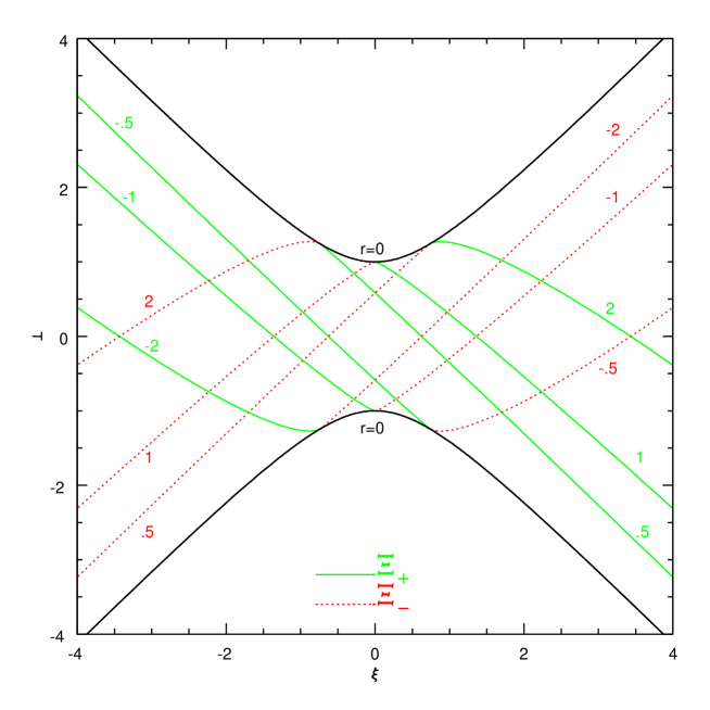
Figure 1: The $\Xi$ constant coordinate surfaces in the Kruskal coordinates. Each of those surfaces is a flat spatial slice. All begin at the r=0 singularity and go out to infinity. Note that both the $\Xi_{+}$ and the $\Xi_{-}$ constant surfaces are spatial surfaces.

Then the Synge coordinates are plotted vs the SK coordinates. The surfaces of constant Synge time $T$ are given in terms of the SK coordinates parametrically by

$${V+U\over 2}(T) = {Te^{r\over 2}\over\sqrt{r}+{\rm asinh(\sqrt{r-1})\over\sqrt{r-1}}}$$ (67)

$${V-U\over 2}(T) = \sqrt{({V+U\over 2})^{2}+(r-1)e^{r}}$$ (68)

where $r$ must be large enough that $V-U\over 2$ is real.

The $\xi$ coordinate constant surfaces are given by

$${V-U\over 2}(\xi)={\xi e^{r\over 2}\over\sqrt{r}+{\rm asinh(\sqrt{r-1})\over\sqrt{r-1}}}$$ (69)

$${V+U\over 2}(\xi)=\pm\sqrt{({(V-U)\over 2})^{2}-(r-1)e^{r}}$$ (70)

where the parameter $r$ is chosen small enough so that ${V+U\over 2}(\xi)$ is real.

In figure 2 we have the plot of the $T$ and $\xi$ constant surfaces in the SK coordinates.

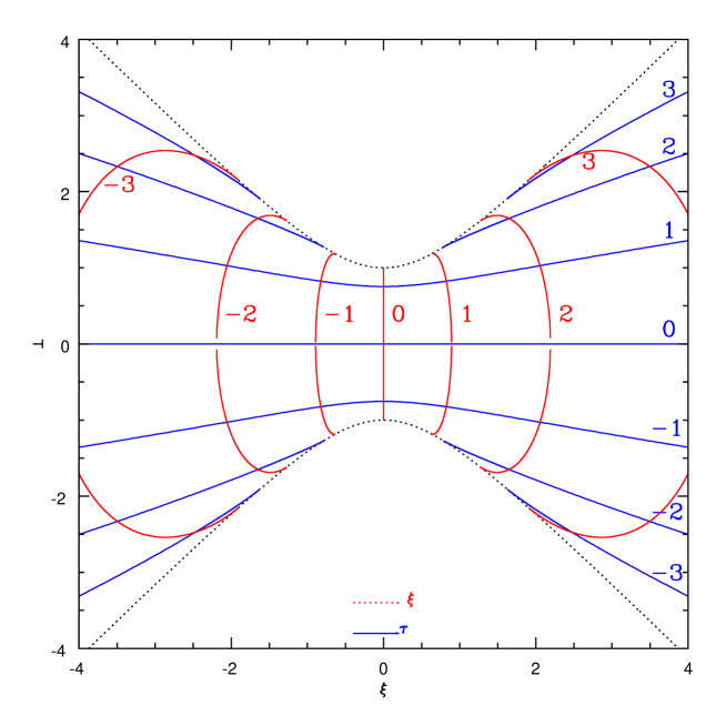
Figure 2: The $T,\xi$ constant coordinate surfaces plotted in Kruskal coordinates. Note that while the $T$ constant hypersurfaces are spacelike hypersurfaces, the $\xi$ constant one as not everywhere timelike. In particular near and within the horizon these surface become timeline for large enough values of $\xi$.

The Lemaître coordinates are interesting because they look, at first, as though they are regular coordinates already which cover the whole spacetime. The metric

$$ds^{2}=d\tau^{2}-{1\over r(\sigma-t)}d\sigma^{2}-r(\sigma-t)^{2}(d\theta^{2}-\sin(\theta)^{2}d\phi^{2})$$ (71)

looks regular everywhere.except at $r=0$ of $t=\sigma$. But if we look at the null geodesics

$${d\sigma\over d\tau}=\pm\sqrt{(}r(\tau-\sigma))=\pm({3\over 2}(\sigma-\tau))^{1\over 3}$$ (72)

we find for the + sign, taking $z=\sigma-\tau$ that

$${dz\over d\tau}=\pm({3\over 2}z)^{1\over 3}-1$$ (73)

The RHS goes to 0 when $z={2\over 3}$ and $\tau$ goes to $\infty$ if we take the $+$ sign in the equation for $z$. Ie, the null geodesics coming out of the black hole come from $\tau\rightarrow-\infty$. Had one taken the other solution ( with $\tau\rightarrow-\tau$) for the Lemaître metric, it would be the ingoing null geodesics which would have terminated at $r=1$. Ie, again the Lemaître coordinates cover only a part of the complete spacetime. The extended Lemaître coordinates ($\Sigma_{\pm}$) do cover the whole of the spacetime.

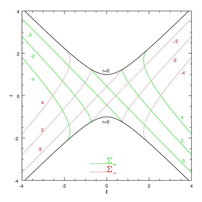
Figure 3: The Lemaitre extended coordinates plotted on the SK extended coordinates.

From the two graphs, of the extended PG coordinates, and the extended Lemaître coordinates, we can see the problem with the original Lemaâitre coordinates. The latter are essentially using the $\Xi_{-}$ and the $\Sigma_{-}$ coordinates. the problem with these is they become degenerate along the past horizon, where both are equal to zero. Ie, these ( and the original Lemaître coordinates which are the logarithm of these coordinates) coordinates do not cover the past horizon. However, if we choose for example the $\Sigma_{+}$ and the $\Xi_{-}$ coordinates, these do cover the whole of the extended spacetime, with no degeneracies. We have

$$\Sigma_{+}\Xi_{-}={\sqrt{r}-1\over\sqrt{r}+1}e^{\sqrt{r}({1\over 3}r+1)}$$ (74)

$${\Sigma_{+}\over\Xi_{-}}=e^{t}e^{{1\over 3}r\sqrt{r}}$$ (75)

or

$${\sqrt{r}(r+2)\over 2(r-1)}dr={d\Sigma_{+}\over\Sigma_{+}}+{d\Xi_{-}\over\Xi_{-}}$$ (76)

$$dt+{1\over 2}\sqrt{r}dr={d\Sigma_{+}\over\Sigma_{+}}-{d\Xi_{-}\over\Xi_{-}}$$ (77)

to give

$$ds^{2}={\sqrt{r}+1\over(r+1)^{2}}\left[(\sqrt{r}+1)e^{-(r/3+2)\sqrt{r}}(\Xi_{-}^{2}d\Sigma_{+}^{2}-\Sigma_{+}^{2}d\Xi_{-}^{2})+4d\Xi_{-}d\Sigma_{+}\right]+r^{2}(d\theta^{2}+\sin(\theta)^{2}d\phi^{2}$$ (78)

This shares with the original Lemaître coordinates that each of the $\Sigma$ constant hypersurfaces are flat three dimensional spatial metrics, while each of the $\Xi,\theta\phi$ constant lines are timelike geodesics which have zero velocity at infinity. Unlike the original Lemaître coordinates however, they cover the whole of the analytic extension of Schwarzschild spacetime. They are thus just as simply married to the flat Robertson Walker dust universe model as were the original Lemaitre coordinates.

Finally, using the Fronsdale coordinates $\Theta,Y$ we plot the $\Theta$ constant and $Y$ constant hypersurfaces. Note that these $\Theta$ constant hypersurfaces surfaces do not run into the $r=0$ singularity. On the other hand, all of the $Y$ constant lines originate at $T=\pm 1,~{}\xi=0$ points on the singularity, with the $Y$ constant lines only being timelike for certain values of $Y<2$ and only for certain values of $\Theta$. Ie, the $Y$ constant coordinate in these “Fronsdale” coordinates is very badly behaved near the $r=0$ singularity while the $\Theta$ const. coordinate surfaces are nicely behaved.

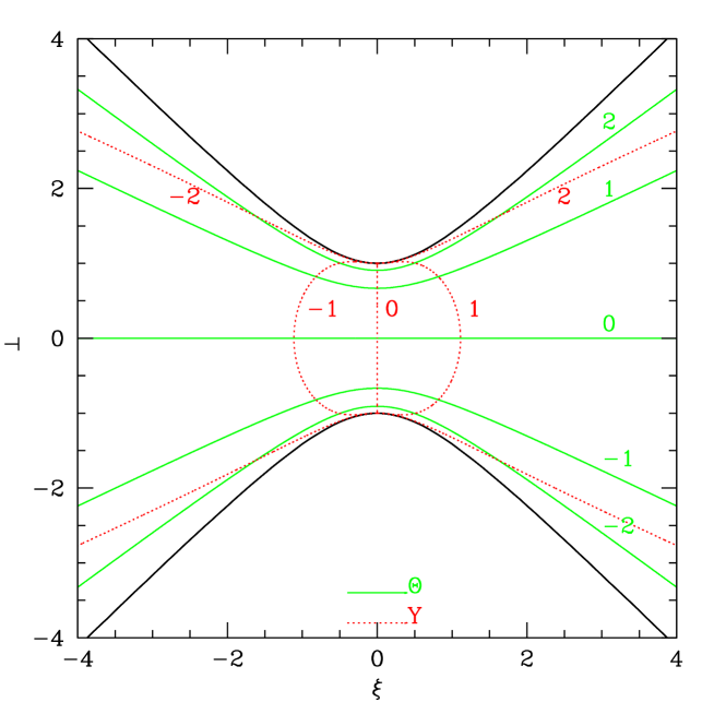
Figure 4: The $\Theta$ and $Y$ constant hypersurfaces for the Fronsdale embedding of Schwarzschild into a flat 6 dimensional spacetime, While the $Y$ constant coordinates seem to hit the $r=0$ singularity are various points, those surfaces actually skirt (as spacelike surfaces) extremely close to the singularity before finally all hitting it at the same point.

References

(1) Schwarzschild, K. (1916). ӆber das Gravitationsfeld eines
Massenpunktes nach der Einsteinschen Theorie”. Sitzungsberichte der Königlich
Preussischen Akademie der Wissenschaften 7: 189-196. For the modern form of
this metric see Droste, J.
(1917). ”On the field of a single centre in Einstein’s theory of gravitation,
and the motion of a particle in that field”. Proceedings Royal Academy
Amsterdam 19 (1): 197?215.
(2) See for example Eisenstaedt, J “The Schwarzschild Solution” in Einstein and the History of General Relativity ed D. Howard, J. Staechel
(1989) Birkhäuser (Boston)
(3) E. Kasner “Finite Representations of the Solar Gravitational
Field in flat space of six dimension” Am. J. Math. 43 130 (1921)
(5)Finkelstein, David (1958). Phys. Rev 110: 965-967
url=http://prola.aps.org/abstract/PR/v110/i4/p965_1
(6)Paul Painlevé, ”La mècanique classique et la théorie de la
relativité”, C. R. Acad. Sci. (Paris) 173, 677-680(1921) Allvar Gullstrand,
”Allgemeine Lösung des statischen Einkörperproblems in der Einsteinschen
Gravitationstheorie”, Arkiv. Mat. Astron. Fys. 16(8), 1-15 (1922)
(7)G. Lemaître (1933). Annales de la Société Scientifique de
Bruxelles A53: 51-85
(8)J. L. Synge, Proc. Roy. Irish Acad., 50, 83 (1950).
(9)
G. Szekeres,Publicationes Mathematicae Debrecen 7, 285
(1960) [submitted May 26, 1959] reprinted in Gen. Rel. Grav., 34, 2001 (2002)
Kruskal, M. (1960). ”Maximal Extension of Schwarzschild Metric”.
Physical Review 119 (5): 1743. [submitted Dec 21, 1959 although reported at
conference June 1959]
Both reference the Synge paper above.
(10) C. Fronsdal, Phys. Rev.,116 778
(1959). See also S.A. Paston, A.A. Sheykin
”Embeddings for Schwarzschild metric classification and new results” Class.
Quant. Grav. 29 095022 (2012) and Arxiv:grqc/1202.1204