Nonlocal Quantum Effects in Cosmology

Abstract

Since it is commonly believed that the observed large-scale structure of the Universe is an imprint of quantum fluctuations existing at the very early stage of its evolution, it is reasonable to pose the question: Do the effects of quantum nonlocality, which are well established now by the laboratory studies, manifest themselves also in the early Universe? We try to answer this question by utilizing the results of a few experiments, namely, with the superconducting multi-Josephson-junction loops and the ultracold gases in periodic potentials. Employing a close analogy between the above-mentioned setups and the simplest one-dimensional Friedmann–Robertson–Walker cosmological model, we show that the specific nonlocal correlations revealed in the laboratory studies might be of considerable importance also in treating the strongly-nonequilibrium phase transitions of Higgs fields in the early Universe. Particularly, they should substantially reduce the number of topological defects (e.g., domain walls) expected due to independent establishment of the new phases in the remote spatial regions. This gives us a hint for resolving a long-standing problem of the excessive concentration of topological defects, inconsistent with observational constraints. The same effect may be also relevant to the recent problem of the anomalous behavior of cosmic microwave background fluctuations at large angular scales.

1. Introduction

The concept of quantum nonlocality originates actually from the paper by Einstein, Podolsky, and Rosen (EPR) Einstein et al. (1935), who posed the problem of correlation between the measurements of two physical objects located in the causally-disconnected regions of space, i.e., beyond the light cones of each other. In the modern and most frequently used in the experiments form, this phenomenon can be illustrated in Figure 1. Here, an original particle of zero spin decays at the instant $t=0$ into two particles with equal but oppositely-directed spins $s_{1}$ and $s_{2}$, which subsequently move from each other in the opposite directions. Next, if measurements of the spins of both particles are performed in the remote spatial points $x_{1}$ and $x_{2}$ at the same instant of time, their values turn out to be perfectly correlated ($s_{1}=-s_{2}$) just because of the law of spin conservation.

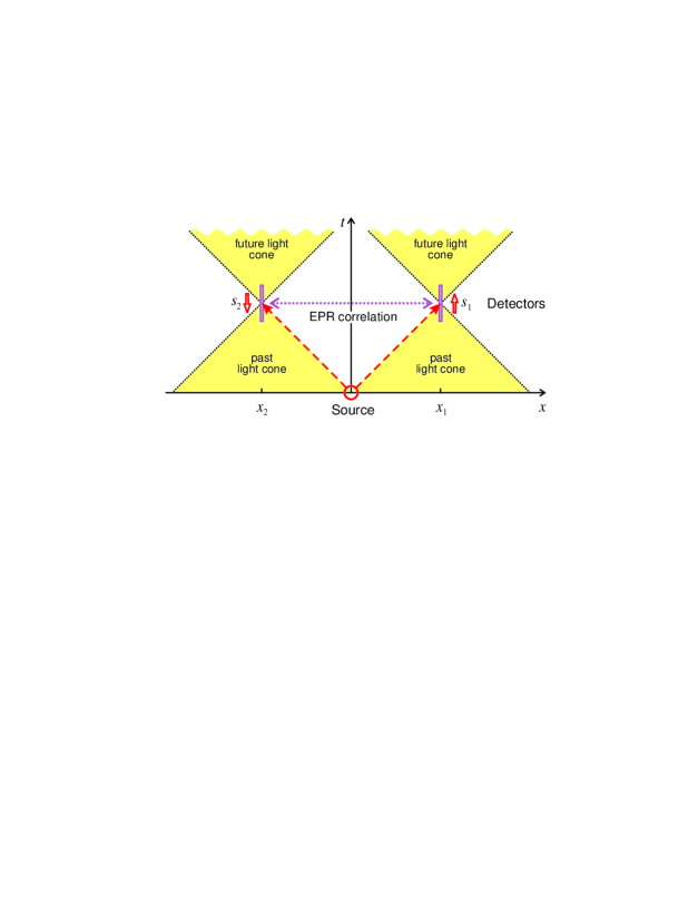
Figure 1: Sketch of the typical laboratory ERP experiment.

At first sight, such correlation is quite surprising, because the measurements are performed in the spots of space–time lying beyond the mutual light cones (i.e., in the causally disconnected regions). However, the existence of EPR correlations is well confirmed now by a lot of laboratory experiments. In fact, these correlations look much less surprising if we keep in mind the fact that both light cones include the same common source in the past. It might be reasonable to emphasize also that, despite of a “superluminal” character of the EPR correlations, they cannot be employed for a faster-than-light communication, because the outcomes of correlated measurements of $s_{1}$ and $s_{2}$ in the points $x_{1}$ and $x_{2}$ are random.

Turning attention to cosmology, we should first of all mention that it is widely believed now that the observed large-scale structure of the Universe is an imprint of quantum fluctuations existing at the very early stages of cosmological evolution. Therefore, it becomes interesting to pose the question: Can the effects of quantum nonlocality, similar to EPR correlations, manifest themselves also in cosmology? In particular, it should be kept in mind that Higgs field, filling the entire Universe and giving masses to the elementary particles, represents actually a kind of Bose–Einstein condensate (BEC), i.e., a macroscopic quantum state, in which the specific quantum correlations may naturally occur.

The most important feature in temporal dynamics of the Higgs field is phase transition caused by the evolving temperature of the Universe, which can finally result in the formation of the nontrivial states of the physical vacuum Linde (1979). In fact, the problem of complex vacuum was recognized long time ago, just after appearance of the idea of spontaneous symmetry breaking in the quantum field theory. Particularly, at the Conference on the occasion of the 400th anniversary of Galileo Galilei’s birth, held in Pisa in 1964, Bogoliubov emphasized that “it is hard to admit, for example, that the ‘phases’ are the same everywhere in the space. So it appears necessary to consider such things as ‘domain structure’ of the vacuum” Bogoliubov (1966). In the next decade, the problem of formation of the domain walls in the course of cosmological evolution was considered in much detail in the work by Zeldovich, Kobzarev, and Okun Zel’dovich et al. (1974) and later in papers by many other authors. (A quite comprehensive overview of the domain wall dynamics was given, for example, in paper Gelmini et al. (1989).)

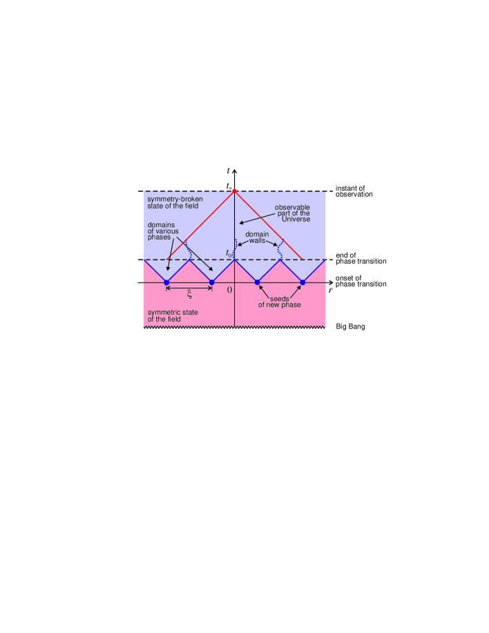
Figure 2: Sketch of development of the phase transition in the expanding Universe.

A commonly-accepted scenario of formation of the domain walls by the phase transition in the early Universe is illustrated in Figure 2. A uniform initial (“symmetric”) state of the Higgs field, existing soon after the Big Bang, cools down due to expansion of the Universe; so that the symmetric phase of the field becomes energetically unfavorable, and the seeds of a new (“symmetry-broken”) phase emerge in some spatial points. (For the sake of simplicity, we shall assume that these points are equally separated along the coordinate $r$ and originate at the same instant of time $t=0$.) Since the seeds of the low-temperature phase emerge independently in the remote spatial regions, their states of the degenerate vacuum, in general, will be different from each other.

Then, the domains of the new phase quickly grow in the course of time and at the instant $t=t_{0}$ collide with each other. However, if the values of the symmetry-broken phase in two neighboring domains were different, they cannot merge smoothly. Instead, a stable topological defect—domain wall (or “kink”)—should be formed at their boundary. So, if the initial separation between the seeds of the new phase was $\xi$, then the resulting concentration of the domain walls can be roughly estimated as $n\approx 1/{\xi}$. This is the so-called Kibble–Zurek (KZ) mechanism for the formation of topological defects after the strongly-nonequilibrium phase transformations Kibble (1976); Zurek (1985).

Strictly speaking, the scenario outlined in Figure 2 refers to the simplest case of Higgs field, possessing ${\mathbb{Z}}_{2}$ symmetry group (i.e., admitting a discrete symmetry breaking). However, the same basic idea is applicable also to more realistic Higgs fields with the continuous symmetries, whose breaking can lead to the formation of more complex defects of the vacuum, such as the monopoles and cosmic strings (or vortices). In general, KZ mechanism gives the following estimate for concentration of the topological defects:

$$n\approx 1/\,{\xi}_{\rm eff}^{\,d}\,,$$ (1)

where ${\xi}_{\rm eff}$ is the effective correlation length, i.e., a typical distance between the seeds of the new phase; and $d=$ 3, 2, and 1 for the monopoles, cosmic strings, and domain walls, respectively. (Their concentrations refer evidently to unit volume, area, and length.)

An accurate calculation of the effective correlation length, in general, is a difficult task. However, its upper bound can be obtained from a simple causality argument: ${\xi}_{\rm eff}\leq c\,t_{\rm pt}$, where $c$ is the speed of light, and $t_{\rm pt}$ is the characteristic time from the Big Bang to the instant of phase transition. Next, the time from the Big Bang in Friedmann–Robertson–Walker (FRW) cosmology is estimated as ${\sim}1/H$, where $H$ is the value of Hubble parameter at the respective instant. Consequently,

$${\xi}_{\rm eff}\,\lesssim\,c\,/H_{\rm pt}\,.$$ (2)

At last, substituting (2) into (1), we get:

$$n\,\gtrsim\,\left(H_{\rm pt}/c\right){}^{d}\,,$$ (3)

where $H_{\rm pt}$ is the value of Hubble parameter at the instant of phase transition.

Unfortunately, the lower theoretical bound (3) is inconsistent with the upper bounds following from observations (e.g., review Klapdor-Kleingrothaus and Zuber (1997)). One possible way to mitigate this disagreement is to modify Lagrangian of the field theory under consideration, typically, by introduction of the “biased” vacuum (thereby, a priori removing the degeneracy) Zel’dovich et al. (1974); Gelmini et al. (1989). Yet another conceivable approach, which was not exploited before, is to take into account the nonlocal quantum correlations, which might manifest themselves in the macroscopic BEC.

However, exploiting the idea of macroscopic quantum correlations, one should bear in mind the following two subtle points:

• Firstly, the most of laboratory studies of EPR correlations, performed since the 1970’s, dealt with the microscopic quantum objects (e.g., atoms and photons). There were only a very few number of experiments on the nonlocal correlations in macroscopic systems; and they will be discussed in detail in the next section.

• Secondly, the correlations studied in microscopic objects were always associated with the exact conservation laws (most typically, the conservation of the total spin). In contract to these cases, the macroscopic BECs do not usually obey the suitable conservation laws. Nevertheless, it might be expected that correlations in the macroscopic systems could be caused just by the energetic criteria: if correlated state of a large system possesses less energy than its uncorrelated state, then it should emerge with a greater probability. As will be shown in the next section, a number of recent laboratory experiments support this idea.

2. Review of the Laboratory Experiments

As far as we know, there are by now two groups of experiments confirming the phenomenon of nonlocal correlations in macroscopic BECs. The first of them are the experiments with superconducting multi-Josephson-junction loops (MJJL), which were started in the very beginning of 2000’s Carmi et al. (2000); and the second are the experiments with ultracold gases in the periodic optical potentials, which began a few years later Hadzibabic et al. (2004, 2006).

2.1. MJJL Experiment

A general scheme of the original MJJL experiment Carmi et al. (2000) is shown in Figure 3: A thin quasi-one-dimensional loop was fabricated from the YBa₂Cu₃O${}_{7\text{-}\delta}$ superconductor and contained 214 segments separated from each other by the Josephson junctions (which are the microscopic domains of the same substance but with a higher critical temperature due to defects in the crystalline lattice). The experimental procedure consisted of the numerous cycles of very quick cooling (approximately from 100 K to 77 K) and subsequent heating of the loop and measurement of the resulting electromagnetic response.

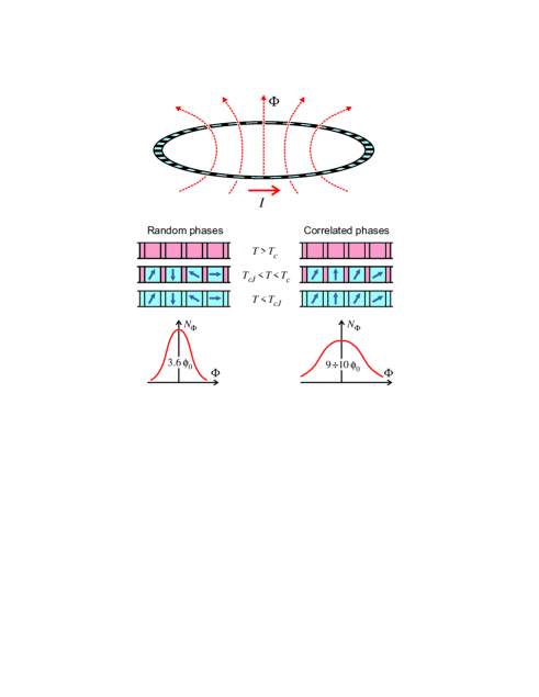
Figure 3: Basic design and principal results of the MJJL experiment.

In the phase of cooling, when temperature $T$ drops approximately to $T_{c}=90$ K, the segments separated by the junctions become superconducting. However, the junctions themselves remain normal and, therefore, the superconducting segments are effectively separated from each other. Consequently, a random phase of the superconducting order parameter should be established in each of them. (They are schematically illustrated in Figure 3 by the randomly oriented arrows.) The total phase variation of the order parameter along the loop, in general, should be nonzero.

At subsequent cooling down to the temperature $T_{cJ}$, which is $5{\div}7$ K below $T_{c}$, the Josephson junctions become also superconducting. Consequently, due to the above-mentioned phase variation, a superconducting current $I$ will develop along the loop. As a result, the loop will be penetrated by the magnetic flux $\Phi$, which is just the measurable quantity. It should be mentioned that this setup is quite close to the original idea by Zurek Zurek (1985), who proposed to observe a spontaneous rotation produced by a rapid phase transition to the superfluid phase in a thin annular tube. Unfortunately, such an experiment was never implemented in practice, since it is hardly possible to observe a mechanical rotation of the macroscopic body with angular momentum of just a few quanta $\hbar$. On the other hand, the magnetic flux measurements by modern apparatus can easily detect the individual quanta of the magnetic flux. Therefore, an electromagnetic analog of the original Zurek’s proposal became feasible.

In summary, because of the phase jumps between the isolated segments formed at the stage when $T_{cJ}<T<T_{c}$, the final magnetic flux $\Phi$ through the loop turns out to be nonzero and varies randomly from one heating–cooling cycle to another. The histogram $N_{\Phi}(\Phi)$ derived from a large number of cycles is well described by the normal (Gaussian) law with zero average value and standard deviation $7.4\,{\phi}_{0}$ (where ${\phi}_{0}$ is the magnetic flux quantum, and $N_{\Phi}$ is the number of cases with the total magnetic flux $\Phi$). This standard deviation is just the typical value of the flux spontaneously generated in one cycle.

In fact, the above-written value is unreasonably large: if the phase jumps between the segments were absolutely independent of each other, then the expected width of the distribution would be only $3.6\,{\phi}_{0}$. However, the excessive value was satisfactorily explained by the authors of the experiment under assumption that phases of the superconducting order parameter in the isolated (i.e., “causally-disconnected”) segments were correlated to each other, so that probability $P({\delta}_{i})$ of the phase jump ${\delta}_{i}$ in the $i$’th junction was given by the Gibbs law:

$$P({\delta}_{i})\propto\exp[-{E_{J}}({\delta}_{i})/k_{B}T]\,,$$ (4)

where $E_{J}$ is the energy concentrated in the Josephson junction, $T$ is the temperature, and $k_{B}$ is Boltzmann constant.

So, the main conclusion following from the above experiment is that the energy concentrated in the defects should be taken into account in the calculation of the probability of realization of various field configurations, even if the phase transformation develops independently in the remote parts of the system.

2.2. Experiments with Ultracold Gases in Optical Lattices

The MJJL experiment, discussed in the previous section, gave the first hint to the importance of using the Gibbs law even for the systems composed of the apparently isolated parts. Unfortunately, this experiment did not enable us to check the particular functional dependence (4). (To do so, it would be necessary to perform the same experiment with different types of superconductors, which has not been fulfilled by now.)

Nevertheless, a few yeas later it became possible to solve this tack by using the BECs of ultracold gases in periodic potentials (or the so-called optical lattices), formed by the intersecting laser beams. These systems represent a close analog of the multiple Josephson junctions and, as distinct from the solid-state setups, their parameters can be easily varied. A diagnostics of the phase jumps in such installations is performed by a removal of the external potential, thereby enabling the pieces of BEC to expand and interfere with each other.

For example, an array of 30 BECs of the ultracold gas in a regular one-dimensional lattice was created in the experiment Hadzibabic et al. (2004). Next, it was demonstrated that such condensates can well interfere with each other even if they were produced independently, i.e., “have never seen one another”.

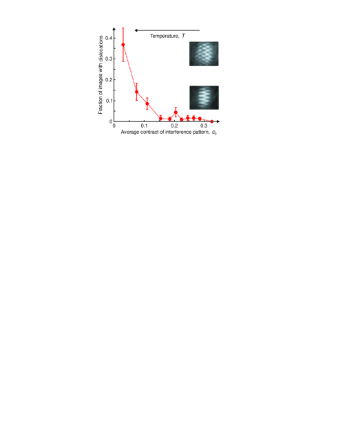
Figure 4: Fraction of the interference patterns showing at least one dislocation as function of the interference contrast $c_{0}$. Inset, examples of images with the increasing number of dislocations (from bottom to top). Adapted by permission from Macmillan Publishers Ltd: Nature, vol. 441, no. 7097, pp. 1118–1121, ©2006.

A further experiment of the same group Hadzibabic et al. (2006) was devoted to a detailed study of the phase defects. In particular, an efficiency of the defect formation was measured as function of temperature. (In fact, the determination of temperature is not an easy task in the experiments with ultracold gases. So, the primary independent parameter was taken to be the average contract of the interference pattern $c_{0}$, which is, roughly speaking, inversely proportional to the temperature $T$.) As a result, it was found that the number of defects (dislocations) formed in the BEC of ultracold gas increases with temperature by qualitatively the same law as (4); see Figure 4 (a sharp outlier at $c_{0}\approx 0.2$ is most probably an experimental inaccuracy).

Therefore, both the MJJL and ultracold-atom experiments suggest that the probability of realization of various configurations of the BEC order parameter should be calculated taking into account the total energy of the system even if separate parts of this system do not interact with each other during a particular physical process (e.g., the phase transformation). Of course, these parts of the system must be causally connected during its previous evolution. This is always satisfied in the laboratory experiments but requires a special consideration in the cosmological context.

In some sense, the above phenomenon can be interpreted as analog of EPR correlation for the system that does not posses an exact conservation law. In such a case, just the energetic criteria should come into play (see also discussion in the end of Section 1).

3. Cosmological Implications

There is evidently a close similarity between the symmetry-breaking phase transitions in the multi-Josephson-junction loop, depicted in Figure 3, and in the simplest one-dimensional (1D) Friedmann–Robertson–Walker (FRW) cosmological model, schematically illustrated in Figure 5. For the sake of definiteness, we shall consider only the simplest type of defects, namely, the domain walls or kinks.

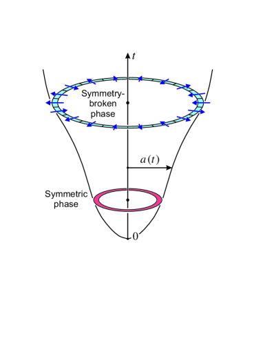
Figure 5: Sketch of the phase transition in 1D FRW cosmological model (the physical distance is measured along the circles).

To make the quantitative estimates, let us consider the space–time metric

$$ds^{2}=\>dt^{2}-\,a^{2}(t)\>dx^{2}\,,$$ (5)

where $t$ is the time, $x$ is the spatial coordinate, and $a(t)$ is the scale factor of FRW model. (From here on, we shall assume that $c\!\equiv\!1$.) Let this space–time be filled with the real scalar field $\varphi$, simulating Higgs field in the theory of elementary particles. Its Lagrangian

$${\cal L}\,(x,t)\,=\,\frac{1}{2}\,\big{[}{\left({\partial}_{t}\varphi\right)}^{2}\!-\,{\left({\partial}_{x}\varphi\right)}^{2}\big{]}\,-\>\frac{\lambda}{4}\,{\big{[}\,{\varphi}^{2}\!-\left({\mu}^{2}/\lambda\right)\big{]}}^{2}$$ (6)

possesses $\mathbb{Z}_{2}$ symmetry group, which should be broken by the phase transition.

As is known, the stable low-temperature vacuum states of the field (6) are

$${\varphi}_{0}=\,\pm\,\mu\,/\sqrt{\lambda}\>,$$ (7)

and a transition region between them (domain wall) is described as

$$\varphi\,(x)=\,{\varphi}_{0}\tanh\!\big{[}({\mu}/{\sqrt{2}}\,)\,(x-x_{0})\big{]}\,.$$ (8)

Such a domain wall contains the energy

$$E=\,\frac{2\,\sqrt{2}}{3}\,\frac{{\mu}^{3}}{\lambda}\;.$$ (9)

We shall assume that thickness of the wall, ${\sim}{1/\mu}$, is small in comparison with a characteristic distance between them; i.e., the domain walls can be treated as point-like objects.

Next, it is convenient to introduce the conformal time $\eta=\!\int dt/a(t)\,$. As a result, the space–time metric (5) will take the conformally flat form Misner (1969):

$$ds^{2}=\,a^{2}(t)\,[\,d{\eta}^{2}\!-dx^{2}\,]\,;$$ (10)

so that the light rays ($ds^{2}\!=0$) will represent the straight lines inclined at $\pm\pi/4\,$:

$$x=\pm\,\eta+{\rm const}\,.$$ (11)

The entire structure of the space–time can be conveniently described by the conformal diagram in Figure 6. Let $\eta\!=\!0$ and $\eta\!=\!{\eta}_{0}$ be the beginning and end of the phase transition, respectively, and $\eta\!=\!{\eta}_{*}$ be the instant of observation. Since it is commonly assumed that bubbles of the new phase grow at the rate close to the speed of light, their boundaries can be well depicted by the light rays. Then, as follows from a simple geometric consideration,

$$N\,=\,({\eta}_{*}\!-{\eta}_{0})/{\eta}_{0}\,\approx\,{\eta}_{*}/{\eta}_{0}\quad(\text{at large }N)$$ (12)

is the number of spatial subregions in the observable Universe causally-disconnected during the phase transition. Their final vacuum states can be conveniently denoted by the arrows, like spins.

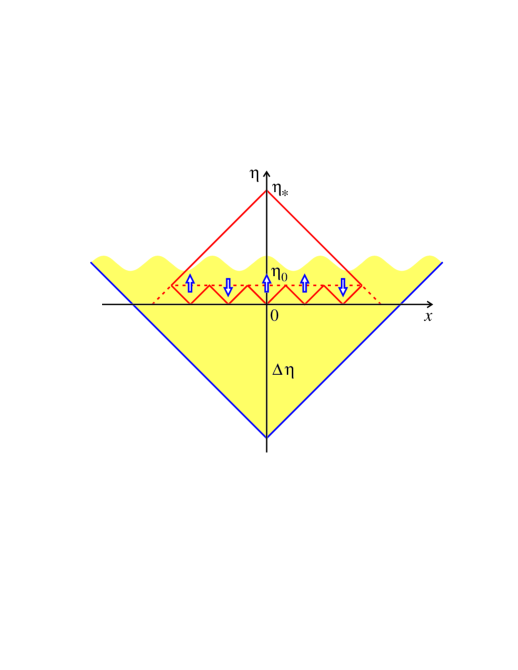
Figure 6: Conformal diagram of 1D FRW cosmological model.

Let us calculate a probability of the phase transition without formation of the domain walls in the observable space–time (the past light cone) $P_{N}^{\,0}$, where subscript $N$ implies the number of subregions; and superscript 0, the absence of domain walls. A trivial estimate can be obtained by taking a ratio of the number of field configurations without domain walls (which equals 2) to their total number ($2^{N}$):

$$P_{N}^{\,0}=\,2\,/\,2^{N}\,=\,1\,/\,2^{N-1}.$$ (13)

This quantity evidently tends to zero very quickly at large $N$. In other words, the observable part of the Universe, represented by the large upper triangle in Figure 6, will inevitably contain some number of the domain walls. Unfortunately, as was recognized long time ago Zel’dovich et al. (1974); Gelmini et al. (1989), a presence of the domain walls is incompatible with astronomical observations.

A possible resolution of this paradox can be based just on taking into consideration the nonlocal Gibbs-like correlations (4). First of all, we must ensure that such correlations can really develop, i.e., the subdomains of the new phase were causally connected in the past. As is seen in Figure 6, this is really possible if a sufficiently long interval of the conformal time

$$\Delta\eta\,\geq\,{\eta}_{*}$$ (14)

preceded the phase transition. Then, the lower shaded triangle will cover at the instant $\eta\!=\!0$ the upper triangle, representing the observable part of the Universe.

The inequality (14) can be satisfied, particularly, in the case of sufficiently long inflationary (de Sitter) stage. Really, if $\,a(t)\propto\exp(Ht)$, where $H$ is Hubble constant, then

$$\eta\,\propto\,-\,\frac{1}{H}\,e^{-Ht}+{\rm const}\,\to\,-\infty\quad\text{at}\quad t\,\to\,-\infty\,;$$ (15)

so that the above-mentioned interval $\Delta\eta$ can be sufficiently large. Let us remind that, from the viewpoint of elementary-particle physics, the de Sitter stage can be naturally realized in the overcooled state of the Higgs field immediately before its first-order phase transition; and just this idea was the starting point of the first inflationary models Linde (1984).

Next, if the condition (14) is satisfied, then it is reasonable to assume that the above-mentioned correlations (4) should take place between the all $N$ subdomains drawn in the conformal diagram, Figure 6. (It is interesting to mention that in our old work Dumin (2000), performed before the MJJL experiment, the same Gibbs-like correlations were introduced on the basis of some metaphysical speculations.) In such a case, the probability $P_{N}^{\,0}$ should be calculated taking into account Gibbs factors for the field configurations involving the domain walls:

$$P_{N}^{\,0}\,=\,2\,/\,Z\>,$$ (16)

where

$$Z\,=\>\sum_{i=1}^{N}\;\sum_{s_{i}=\pm 1}\exp\bigg{\{}\!-\frac{E}{T}\,\sum_{j=1}^{N}\,\frac{1}{2}\,(1-\,s_{j}\,s_{j+1})\bigg{\}}\,.$$ (17)

Here, $s_{j}$ is the spin-like variable denoting a sign of the vacuum state in the $j$’th subdomain, $E$ is the domain wall energy, given by (9), and $T$ is the characteristic temperature of the phase transition. (From here on, the temperature will be expressed in energetic units; so the Boltzmann constant $k_{B}$ will be omitted.)

From a formal point of view, statistical sum (17) is very similar to the sum for Ising model, well studied in the physics of condensed matter, e.g. Isihara (1971). Using exactly the same mathematical approach, we get the final result:

$$P_{N}^{\,0}\,=\,\frac{2}{{\left[1+e^{-E/T}\right]}^{N}+{\left[1-e^{-E/T}\right]}^{N}}\;.$$ (18)

(Yet another method for calculation of the same quantity, which is more straightforward and pictorial but less informative, can be found in Dumin (2000); the approach outlined here was employed for the first time in our paper Dumin (2003).)

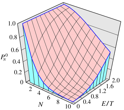
Figure 7: The probability of phase transition without formation of the domain walls $P_{N}^{\,0}$ as function of the number of disconnected subregions $N$ and the ratio of the domain wall energy to the phase transition temperature $E/T$.

The quantity $P_{N}^{\,0}$ as function of $N$ and $E/T$ is plotted in Figure 7. It is seen that $P_{N}^{\,0}$ drops very sharply with increase in $N$ at small values of $E/T$ (when the effect of Gibbs-like correlations is insignificant), but it becomes a gently decreasing function of $N$ when the parameter $E/T$ is sufficiently large. Some other plots illustrating suppression of concentration of the domain walls by the nonlocal correlations can be found in paper Dumin (2009), devoted to the phase transformations in superfluids and superconductors. Therefore, just the large energy concentrated in the domain walls turns out to be the factor substantially reducing the probability of their creation.

Next, as can be easily derived from (18), the probability of absence of the domain walls in the observable Universe becomes on the order of unity, e.g. 1/2, if $\,E/T\gtrsim\ln N$. Taking into account (9) and (12), this inequality can be rewritten as

$$\frac{{\mu}^{3}}{\lambda\,T}\>\gtrsim\>\ln\frac{{\eta}_{*}}{{\eta}_{0}}\>.$$ (19)

Because of the very weak logarithmic dependence in the right-hand side, such a condition could be reasonably satisfied for a certain class of field theories.

Moreover, the situation becomes even more favorable in the case of two- or three-dimensional space. The point is that a well-known property of the 2D and 3D Ising models is a tendency for aggregation of the domains with the same value of the order parameter when the temperature drops below some critical value $T_{c}\sim E$ Rumer and Ryvkin (1980). In the condensed-matter applications, this corresponds, for example, to the spontaneous magnetization of a solid body. Regarding the cosmological context, one can expect that probability of formation of the domain walls will be reduced dramatically at the sufficiently large values of $E/T$; some illustrations of this phenomenon can be found in Dumin (2009). (To avoid misunderstanding, let us emphasize that the above-mentioned Ising models are only the auxiliary mathematical constructions, describing a final distribution of the domain walls after the phase transformation. So, the formal phase transitions in the 2D and 3D Ising models should not be associated with the physical phase transition in the original ${\varphi}^{4}$-field model (6); for more details, see Table 2 in Dumin (2009).)

4. Discussion and Conclusions

As was discussed in the present article, a few laboratory experiments suggest a presence of the nonlocal Gibbs-like correlations between the phases of BECs after the rapid phase transformations. Therefore, it can be reasonably conjectured that the same correlations should occur in the BEC of Higgs field, which is formed in the course of evolution of the Universe. As follows from our quantitative estimates for the simplest case of 1D FRW cosmological model, such correlations can show a way to resolve the well-known problem of the excessive concentration of the domain walls resulting from phase transitions in the early Universe. In fact, this problem was recognized in the mid 1970s Zel’dovich et al. (1974); and since that time a commonly-used approach to its resolution was based on the introduction of the so-called “biased” (or asymmetric) vacuum. As a result, under the appropriate choice of parameters, the regions of “false” (energetically unfavorable) vacuum should quickly disappear, eliminating the corresponding domain walls Gelmini et al. (1989). Unfortunately, the concept of biased vacuum was not supported by independent data in the physics of elementary particles. On the other hand, the idea of nonlocal correlations, employed in the present study, is supported by at least a few laboratory experiments. Therefore, from our point of view, it looks more attractive.

It should be emphasized again that a number of arguments from the modern observational cosmology impose severe constraints on the concentration of domain walls. In particular, an appreciable number of the domain walls would produce an unacceptable anisotropy of the cosmic microwave background (CMB) radiation, change the overall rate of the cosmological expansion, etc. Besides, it is commonly believed now that the primordial spectrum of density fluctuations, responsible for the formation of the large-scale structure, is formed by the Gaussian quantum fluctuations in the very early Universe amplified by the subsequent inflationary stage, while contribution from the topological defects is quite insignificant. All these facts imply that there should be an efficient mechanism for the suppression of the domain walls, and the nonlocal quantum correlations discussed in the present paper might be a reasonable option.

Yet another recent cosmological problem, recognized due to WMAP and confirmed by the Planck satellite data, is the anomalous behaviour of CMB fluctuations at large angular scales, approximately over $10^{\rm o}$ Wright (2013); Hofmann (2013). It can be conjectured that such anomalies are associated just with the nonlocal correlations in the early Universe; but, of course, a much more elaborated analysis must be performed to draw a reliable conclusion.

At last, we would like to mention a recent activity in the experiments with ultracold gases for simulation of various dynamical phenomena in cosmology, e.g., the so-called Sakharov oscillations Schmiedmayer and Berges (2013). From our point of view, a more careful study of the nonlocal correlations may become an important branch in this rapidly-growing research field.

References

- Einstein et al. (1935) A. Einstein, B. Podolsky, and N. Rosen, “Can quantum-mechanical description of physical reality be considered complete?” Physical Review, vol. 47, no. 10, pp. 777–780, 1935.
- Linde (1979) A.D. Linde, “Phase transitions in gauge theories and cosmology,” Reports on Progress in Physics, vol. 42, no. 3, pp. 389–437, 1979.
- Bogoliubov (1966) N.N. Bogoliubov, “Field-theoretical methods in physics,” Supplemento al Nuovo Cimento (Serie prima), vol. 4, no. 2, pp. 346–357, 1966.
- Zel’dovich et al. (1974) Ia.B. Zeldovich, I.Yu. Kobzarev, and L.B. Okun, “Cosmological consequences of a spontaneous breakdown of a discrete symmetry,” Soviet Physics—JETP, vol. 40, no. 1, pp. 1–5, 1975 [Translated from: Zhurnal Eksperimental’noi i Teoreticheskoi Fiziki, vol. 67, p. 3–11, 1974].
- Gelmini et al. (1989) G.B. Gelmini, M. Gleiser, and E.W. Kolb, “Cosmology of biased discrete symmetry breaking,” Physical Review D, vol. 39, no. 6, pp. 1558–1566, 1989.
- Kibble (1976) T.W.B. Kibble, “Topology of cosmic domains and strings,” Journal of Physics A: Mathematical and General, vol. 9, no. 8, pp. 1387–1398, 1976.
- Zurek (1985) W.H. Zurek, “Cosmological experiments in superfluid helium?” Nature, vol. 317, no. 6037, pp. 505–508, 1985.
- Klapdor-Kleingrothaus and Zuber (1997) H.V. Klapdor-Kleingrothaus and K. Zuber, Particle Astrophysics, Institute of Physics Publishing, Bristol, 1997.
- Carmi et al. (2000) R. Carmi, E. Polturak, and G. Koren, “Observation of spontaneous flux generation in a multi-Josephson-junction loop,” Physical Review Letters, vol. 84, no. 21, pp. 4966–4969, 2000.
- Hadzibabic et al. (2004) Z. Hadzibabic, S. Stock, B. Battelier, V. Bretin, and J. Dalibard, “Interference of an array of independent Bose–Einstein condensates,” Physical Review Letters, vol. 93, no. 18, Article ID 180403 (4 pp.), 2004.
- Hadzibabic et al. (2006) Z. Hadzibabic, P. Kruger, M. Cheneau, B. Battelier, and J. Dalibard, “Berezinskii–Kosterlitz–Thouless crossover in a trapped atomic gas,” Nature, vol. 441, no. 7097, pp. 1118–1121, 2006.
- Misner (1969) C.W. Misner, “Mixmaster Universe,” Physical Review Letters, vol. 22, no. 20, pp. 1071–1074, 1969.
- Linde (1984) A.D. Linde, “The inflationary Universe,” Reports on Progress in Physics, vol. 47, no. 8, pp. 925–986, 1984.
- Dumin (2000) Yu.V. Dumin, “On a probable role of EPR (Einstein–Podolsky–Rosen) correlations in breaking the symmetry of Higgs fields in cosmological phase transitions,” Hot Points in Astrophysics: Proceedings of the International Workshop, pp. 114–120, Joint Institute for Nuclear Research, Dubna, 2000.
- Isihara (1971) A. Isihara, Statistical Physics, Academic Press, New York, 1971.
- Dumin (2003) Yu.V. Dumin, “On the influence of Einstein–Podolsky–Rosen effect on the domain wall formation during the cosmological phase transitions,” Frontiers of Particle Physics: Proceedings of the Tenth Lomonosov Conference on Elementary Particle Physics, pp. 289–294, World Scientific Publishing Co., Singapore, 2003.
- Dumin (2009) Yu.V. Dumin, “Ultracold gases and multi-Josephson junctions as simulators of out-of-equilibrium phase transformations in superfluids and superconductors,” New Journal of Physics, vol. 11, no. 10, Article ID 103032 (12 pp.), 2009.
- Rumer and Ryvkin (1980) Yu.B. Rumer and M.Sh. Ryvkin, Thermodynamics, Statistical Physics, and Kinetics, Mir, Moscow, 1980.
- Wright (2013) A. Wright, “Across the Universe,” Nature Physics, vol. 9, no. 5, p. 264, 2013.
- Hofmann (2013) R. Hofmann, “The fate of statistical isotropy,” Nature Physics, vol. 9, no. 11, pp. 686–689, 2013.
- Schmiedmayer and Berges (2013) J. Schmiedmayer and J. Berges, “Cold atom cosmology,” Science, vol. 341, no. 6151, pp. 1188–1189, 2013.