Binary Classifier Calibration: Non-parametric approach

Abstract

Accurate calibration of probabilistic predictive models learned is critical for many practical prediction and decision-making tasks. There are two main categories of methods for building calibrated classifiers. One approach is to develop methods for learning probabilistic models that are well-calibrated, ab initio. The other approach is to use some post-processing methods for transforming the output of a classifier to be well calibrated, as for example histogram binning, Platt scaling, and isotonic regression. One advantage of the post-processing approach is that it can be applied to any existing probabilistic classification model that was constructed using any machine-learning method.

In this paper, we first introduce two measures for evaluating how well a classifier is calibrated. We prove three theorems showing that using a simple histogram binning post-processing method, it is possible to make a classifier be well calibrated while retaining its discrimination capability. Also, by casting the histogram binning method as a density-based non-parametric binary classifier, we can extend it using two simple non-parametric density estimation methods. We demonstrate the performance of the proposed calibration methods on synthetic and real datasets. Experimental results show that the proposed methods either outperform or are comparable to existing calibration methods.

1 Introduction

The development of accurate probabilistic prediction models from data is critical for many practical prediction and decision-making tasks. Unfortunately, the majority of existing machine learning and data mining models and algorithms are not optimized for this task and predictions they produce may be miscalibrated.

Generally, a set of predictions of a binary outcome is well calibrated if the outcomes predicted to occur with probability $p$ do occur about $p$ fraction of the time, for each probability $p$ that is predicted. This concept can be readily generalized to outcomes with more than two values. Figure 2 shows a hypothetical example of a reliability curve degroot1983comparison ; niculescu2005predicting , which displays the calibration performance of a prediction method. The curve shows, for example, that when the method predicts $Z=1$ to have probability $0.5$, the outcome $Z=1$ occurs in about $0.57$ fraction of the instances (cases). The curve indicates that the method is fairly well calibrated, but it tends to assign probabilities that are too low. In general, perfect calibration corresponds to a straight line from $(0,0)$ to $(1,1)$. The closer a calibration curve is to this line, the better calibrated is the associated prediction method.

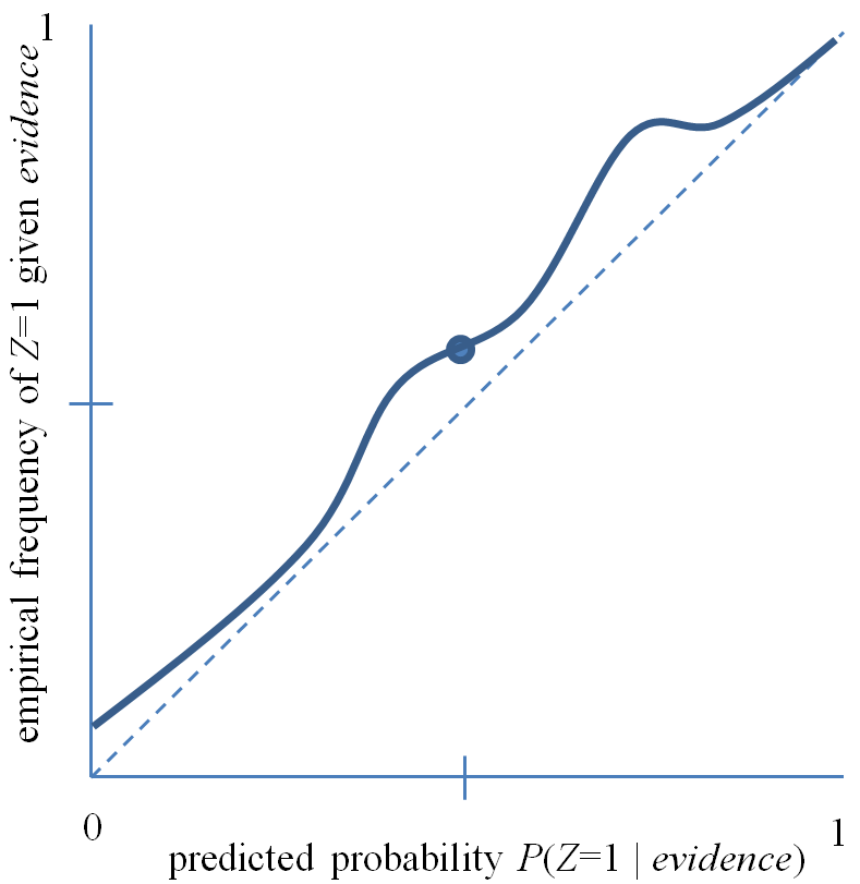
Figure 1: The solid line shows a calibration (reliability) curve for predicting $Z=1$. The dotted line is the ideal calibration curve.

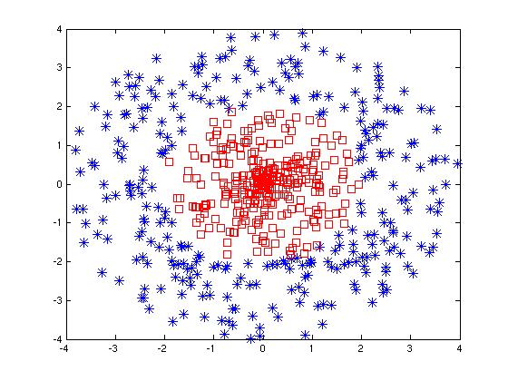
Figure 2: Scatter plot of non-linear separable simulated data

If uncertainty is represented using probabilities, then optimal decision making under uncertainty requires having models that are well calibrated. Producing well calibrated probabilistic predictions is critical in many areas of science (e.g., determining which experiments to perform), medicine (e.g., deciding which therapy to give a patient), business (e.g., making investment decisions), and many other areas. At the same time, calibration has not been studied nearly as extensively as discrimination (e.g., ROC curve analysis) in machine learning and other fields that research probabilistic modeling.

One approach to achieve a high level of calibration is to develop methods for learning probabilistic models that are well-calibrated, ab initio. However, data mining and machine learning research has traditionally focused on the development of methods and models for improving discrimination, rather than on methods for improving calibration. As a result, existing methods have the potential to produce models that are not well calibrated. The miscalibration problem can be aggravated when models are learned from small-sample data or when the models make additional simplifying assumptions (such as linearity or independence).

Another approach is to apply post-processing methods (e.g., histogram binning, Platt scaling, or isotonic regression) to the output of classifiers to improve their calibration. The post-processing step can be seen as a function that maps output of a prediction model to probabilities that are intended to be well calibrated. Figure 2 shows an example of such a mapping. This approach frees the designer of the machine learning model from the need to add additional calibration measures and terms into the objective function used to learn a model. The advantage of this approach is that it can be used with any existing classification method, since calibration is performed solely as the post-processing step.

The objective of the current paper is to show that the post-processing approach for calibrating binary classifiers is theoretically justified. In particular, we show in the large sample limit that post-processing will produce a perfectly calibrated classifier that has discrimination perform (in terms of area under the ROC curve) that is at least as good as the original classifier. In the current paper we also introduce two simple but effective methods that can address the miscalibration problem.

Existing post-processing calibration methods can be divided into parametric and non-parametric methods. An example of a parametric method is Platt’s method that applies a sigmoidal transformation that maps the output of a predictive model platt1999probabilistic to a calibrated probability output. The parameters of the sigmoidal transformation function are learned using a maximum likelihood estimation framework. The key limitation of the approach is the (sigmoidal) form of the transformation function, which only rarely fits the true distribution of predictions.

The above problem can be alleviated using non-parametric methods. The most common non-parametric methods are based either on binning zadrozny2001obtaining or isotonic regression ayer1955empirical . In the histogram binning approach, the raw predictions of a binary classifier are sorted first, and then they are partitioned into $b$ subsets of equal size, called bins. Given a prediction $y$, the method finds the bin containing that prediction and returns as $\hat{y}$ the fraction of positive outcomes $(Z=1)$ in the bin.

Zadronzy and Elkan zadrozny2002transforming developed a calibration method that is based on isotonic regression. This method only requires that the mapping function be isotonic (monotonically increasing) niculescu2005predicting . The pair adjacent violators (PAV) algorithm is one instance of an isotonic regression algorithm ayer1955empirical . The isotonic calibration method based on the (PAV) algorithm can be viewed as a binning algorithm where the position of boundaries and the size of bins are seleted according to how well the classifier ranks the examples in the training data zadrozny2002transforming . Recently a variation of the isotonic-regression-based calibration method was described for predicting accurate probabilities with a ranking lossmenon2012predicting .

In this paper, section 2 introduces two measures, maximum calibration error(MCE) and expected calibration error(ECE), for evaluating how well a classifier is calibrated. In section 3 we prove three theorems to show that by using a simple histogram-binning calibration method, it is possible to improve the calibration capability of a classifier measured in terms of $MCE$ and $ECE$ without sacrificing its discrimination capability measured in terms of area under (ROC) curve ($AUC$). Section 4 introduces two simple extensions of the histogram binning method by casting the method as a simple density based non-parametric binary classification problem. The results of experiments that evaluate various calibration methods are presented in section 5. Finally, section 6 states conclusions and describes several areas for the future work.

2 Notations and Assumptions

This section present the notation and assumptions we use for formalizing the problem of calibrating a binary classifier. We also define two measures for assessing the calibration of such classifiers.

Assume a binary classifier is defined as a mapping $\phi:R^{d}\rightarrow[0,1]$. As a result, for every input instance $x\in R^{d}$ the output of the classifier is $y=\phi(x)$ where $y\in[0,1]$. For calibrating the classifier $\phi(.)$ we assume there is a training set $\{(x_{i},y_{i},z_{i})\}_{i=1}^{N}$ where $x_{i}\in R^{d}$ is the i’th instance and $y_{i}=\phi(x_{i})\in[0,1]$, and $z_{i}\in\{0,1\}$ is the true class of i’th instance. Also we define $\hat{y}_{i}$ as the probability estimate for instance $x_{i}$ achieved by using the histogram binning calibration method, which is intended to yield a more calibrated estimate than does $y_{i}$. In addition we have the following notation and assumptions that are used in the remainder of the paper:

• $N$ is total number of instances

• $m$ is total number of positive instances

• $n$ is total number of negative instances

• $p_{in}$ is the space of uncalibrated probabilities $\{y_{i}\}$ which is defined by the classifier output

• $p_{out}$ is the space of transformed probability estimates $\{\hat{y}_{i}\}$ using histogram binning

• $B$ is the total number of bins defined on $p_{in}$ in the histogram binning model

• $B_{i}$ is the i’th bin defined on $p_{in}$

• $N_{i}$ is total number of instances $x_{k}$ for which the predicted value $y_{k}$ is located inside $B_{i}$

• $m_{i}$ is number of positive instances $x_{k}$ for which the predicted value $y_{k}$ is located inside $B_{i}$

• $n_{i}$ is number of negative instances $x_{k}$ for which the predicted value $y_{k}$ is located inside $B_{i}$

• $\hat{\eta}_{i}=\frac{N_{i}}{N}$ is an empirical estimate of $\mathbb{P}\{y\in B_{i}\}$

• $\eta_{i}$ is the value of $\mathbb{P}\{y\in B_{i}\}$ as $N$ goes to infinity

• $\hat{\theta}_{i}=\frac{m_{i}}{N_{i}}$ is an empirical estimate of $\mathbb{P}\{z=1|y\in B_{i}\}$

• $\theta_{i}$ is the value of $\hat{\theta}_{i}$ as $N$ goes to infinity

2.1 Calibration Measures

In order to evaluate the calibration capability of a classifier, we use two simple statistics that measure calibration relative to the ideal reliability diagram degroot1983comparison ; niculescu2005predicting (Figure 2 shows an example of a reliability diagram). These measures are called Expected Calibration Error (ECE), and Maximum Calibration Error (MCE). In computing these measures, the predictions are sorted and partitioned into ten bins. The predicted value of each test instance falls into one of the bins. The $ECE$ calculates Expected Calibration Error over the bins, and $MCE$ calculates the Maximum Calibration Error among the bins, using empirical estimates as follows:

$$ECE=\sum_{i=1}^{10}P(i)\cdot\left|o_{i}-e_{i}\right| MCE=\max\left(\left|o_{i}-e_{i}\right|\right),$$ ,

where $o_{i}$ is the true fraction of positive instances in bin $i$, $e_{i}$ is the mean of the post-calibrated probabilities for the instances in bin $i$, and $P(i)$ is the empirical probability (fraction) of all instances that fall into bin $i$. The lower the values of $ECE$ and $MCE$, the better is the calibration of a model.

3 Calibration Theorems

In this section we study the properties of the histogram-binning calibration method. We prove three theorems that show that this method can improve the calibration power of a classifier without sacrificing its discrimination capability.

The first theorem shows that the $MCE$ of the histogram binning method is concentrated around zero:

Theorem 3.1.

Using histogram binning calibration, with probability at least $1-\delta$ we have $MCE\leq\sqrt{\frac{2B\log{\frac{2B}{\delta}}}{N}}$.

Proof.

For proving this theorem, we first use a concentration result for $\hat{\theta}_{i}$. Using Hoeffding’s inequality we have the following:

$$\mathbb{P}\{|\hat{\theta}_{i}-\theta|\geq\epsilon\}\leq 2e^{\frac{-2N\epsilon^{2}}{B}}$$ (1)

Let’s assume $\tilde{B}_{i}$ is a bin defined on the space of transformed probabilities $p_{out}$ for calculating the $MCE$ of histogram binning method. Assume after using histogram binning over $p_{in}$ (space of uncalibrated probabilities which is generated by the classifier $\phi$), $\hat{\theta}_{i1},..,\hat{\theta}_{ik_{i}}$ will be mapped into $\tilde{B}_{i}$. We define $o_{i}$ as the true fraction of positive instances in bin $\tilde{B}_{i}$, and $e_{i}$ as the mean of the post-calibrated probabilities for the instances in bin $\tilde{B}_{i}$. Using the notation defined in section 2, we can write $o_{i}$ and $e_{i}$ as follows:

$$o_{i}=\frac{\eta_{i1}\theta_{i1}+\ldots+\eta_{ik_{i}}\theta_{ik_{i}}}{\eta_{i1}+\ldots+\eta_{ik_{i}}},\text{ }e_{i}=\frac{\eta_{i1}\hat{\theta}_{i1}+\ldots+\eta_{ik_{i}}\hat{\theta}_{ik_{i}}}{\eta_{i1}+\ldots+\eta_{ik_{i}}}\\$$

by defining $\alpha_{it}=\frac{\eta_{it}}{\eta_{i1}+\ldots+\eta_{ik_{i}}}$ and using the triangular inequality we have that:

$$|o_{i}-e_{i}|\leq\sum_{t\in\{1,\ldots,k_{i}\}}\alpha_{it}|\hat{\theta}_{it}-\theta_{it}|\text{ }\leq\text{ }max_{t\in\{1,\ldots,k_{i}\}}|\hat{\theta}_{it}-\theta_{it}|$$ (2)

Using the above result and the concentration inequality 7 for $\hat{\theta_{i}}$ we can conclude:

$$\mathbb{P}\{|o_{i}-e_{i}|>\epsilon\} \leq\mathbb{P}\{max_{t\in\{1,\ldots,k_{i}\}}|\hat{\theta}_{it}-\theta_{it}|>\epsilon\}\leq 2k_{i}e^{\frac{-N\epsilon^{2}}{2B}},$$ (3)

Where the last part is obtained by using a union bound and $k_{i}$ is the number of bins on the space $p_{in}$ for which their calibrated probability estimate will be mapped into the bin $\tilde{B}_{i}$.

Using a union bound again over different bins like $\tilde{B}_{i}$ defined on the space $p_{out}$, we achieve the following probability bound for $MCE$ over the space of calibrated estimates $p_{out}$ :

$$\mathbb{P}\{\max_{i=1}^{B}|o_{i}-e_{i}|\geq\epsilon\}\leq 2(K_{1}+\ldots+K_{B})e^{\frac{-N\epsilon^{2}}{2B}}\Longrightarrow\mathbb{P}\{MCE\geq\epsilon\}\leq 2Be^{\frac{-N\epsilon^{2}}{2B}}$$

By setting $\delta=2Be^{\frac{-N\epsilon^{2}}{2B}}$ we can show that with probability $1-\delta$ the following inequality holds $MCE\leq\sqrt{\frac{2B\log{\frac{2B}{\delta}}}{N}}$. ∎

Corollary 3.2.

Using histogram binning calibration method, MCE converges to zero with the rate of $O(\sqrt{\frac{B\log{B}}{N}})$.

Next, we prove a theorem for bounding the ECE of the histogram-binning calibration method as follows:

Theorem 3.3.

Using histogram binning calibration method, ECE converges to zero with the rate of $O(\sqrt{\frac{B}{N}})$.

Proof.

The proof of this theorem uses the concentration inequality 3.Due to space limitations, the details of the proof is stated in the supplementary part of the paper. ∎

The above two theorems show that we can bound the calibration error of a binary classifier, which is measured in terms of $MCE$ and $ECE$, by using a histogram-binning post-processing method. We next show that in addition to gaining calibration power, by using histogram binning we are guaranteed not to sacrifice discrimination capability of the base classifier $\phi(.)$ measured in terms of $AUC$. Recall the definitions of $y_{i}$ and $\hat{y_{i}}$, where $y_{i}=\phi(x_{i})$ is the probability prediction of the base classifier $\phi(.)$ for the input instance $x_{i}$, and $\hat{y}_{i}$ is the transformed estimate for instance $x_{i}$ that is achieved by using the histogram-binning calibration method.

We can define the $AUC\_Loss$ of the histogram-binning calibration method as:

• ($AUC\_Loss$) $AUC\_Loss$ is the difference between the AUC of the base classifier estimate and the AUC of transformed estimate using the histogram-binning calibration method. Using the notation in Section 2, it is defined as $AUC\_Loss=AUC(y)-AUC(\hat{y})$

Using the above definition, our third theorem bounds the $AUC\_Loss$ of histogram binning classifier as follows:

Theorem 3.4.

Using the histogram-binning calibration method, the worst case $AUC\_Loss$ is upper bounded by $O(\frac{1}{B})$.

Proof.

Due to space limitations, the proof of this theorem is stated in the appendix section in the supplementary part of the paper. ∎

Using the above theorems, we can conclude that by using the histogram-binning calibration method we can improve calibration performance of a classifier measured in terms of $MCE$ and $ECE$ without losing discrimination performance of the base classifier measured in terms of $AUC$.

We will show in Section 4 that the histogram binning calibration method is simply a non-parametric plug-in classifier. By casting histogram binning as a non-parametric histogram binary classifier, there are other results that show the histogram classifier is a mini-max rate classifier for Lipschitz Bayes decision boundaries devroye1996probabilistic . Although the results are valid for histogram classifiers with fixed bin size, our experiments show that both fixed bin size and fixed frequency histogram classifiers behave quite similarly. We conjecture that a histogram classifier with equal frequency binning is also a mini-max (or near mini-max) rate classifierscott2003near ; klemela2009multivariate ; this is an interesting open problem that we intend to study in the future. These results make histogram binning a reasonable choice for binary classifier calibration under the condition $B\rightarrow\infty$ and $\frac{N}{B\log{B}}\rightarrow\infty$ as $N\rightarrow\infty$. This could be achieved by setting $B\simeq N^{\frac{1}{3}}$, which is the optimum number of bins in order to have optimal convergence rate results for the non-parametric histogram classifier devroye1996probabilistic .

4 Calibration Methods

In this section, we show that the histogram-binning calibration method zadrozny2001obtaining is a simple nonparametric plug-in classifier. In the calibration problem, given an uncalibrated probability estimate $y$, one way of finding the calibrated estimate $\hat{y}=\mathbb{P}(Z=1|y)$ is to apply Bayes’ rule as follows:

$$\mathbb{P}(Z=1|y)=\frac{P(z=1)\cdot P(y|z=1)}{p(z=1)\cdot P(y|z=1)+P(z=0)\cdot P(y|z=0)},$$ (4)

where $P(z=0)$ and $P(z=1)$ are the priors of class $0$ and $1$ that are estimated from the training dataset. Also, $P(y|z=1)$ and $P(y|z=0)$ are predictive likelihood terms. If we use the histogram density estimation method for estimating the predictive likelihood terms in the Bayes rule equation 4 we obtain the following: $\hat{P}(y|z=t)=\sum_{j=1}^{B}\frac{\hat{\theta}_{j}^{t}}{h_{j}}I(y\in B_{j})$, where $t=\{0,1\}$, $\hat{\theta}_{j}^{0}=\frac{1}{n}\sum_{i=1}^{N}I(y_{i}\in B_{j},z_{i}=0)$, and $\hat{\theta}_{j}^{1}=\frac{1}{m}\sum_{i=1}^{N}I(y_{i}\in B_{j},z_{i}=1)$ are the empirical estimates of the probability of a prediction when class $z=t$ falls into bin $B_{j}$. Now, let us assume $y\in B_{j}$; using the assumptions in Section 2, by substituting the value of empirical estimates of $\hat{\theta_{j}^{0}}=\frac{n_{j}}{n}$, $\hat{\theta_{j}^{1}}=\frac{m_{j}}{m}$, $\hat{P}(z=0)=\frac{n}{N}$, $\hat{P}(z=1)=\frac{m}{N}$ from the training data and performing some basic algebra we obtain the following calibrated estimate: $\hat{y}=\frac{m_{j}}{m_{j}+n_{j}}$, where $m_{i}$ and $n_{j}$ are the number of positive and negative examples in bin $B_{j}$.

The above computations show that the histogram-binning calibration method is actually a simple plug-in classifier where we use the histogram-density method for estimating the predictive likelihood in terms of Bayes rule as given by 4. By casting histogram binning as a plug-in method for classification, it is possible to use more advanced frequentist methods for density estimation rather than using simple histogram-based density estimation. For example, if we use kernel density estimation (KDE) for estimating the predictive likelihood terms, the resulting calibrated probability $P(Z=1|X=x)$ is as follows:

$$\hat{P}(Z=1|X=x)=\frac{nh_{0}\sum_{X_{i}\in X^{+}}K\left(\frac{|x-X_{i}|}{h_{1}}\right)}{nh_{0}\sum_{X_{i}\in X^{+}}K\left(\frac{|x-X_{i}|}{h_{1}}\right)+mh_{1}\sum_{X_{i}\in X^{-}}K\left(\frac{|x-X_{i}|}{h_{0}}\right)},$$ (5)

where $X_{i}$ are training instances, and $m$ and $n$ are respectively the number of positive and negative examples in training data. Also $h_{0}$ and $h_{1}$ are the bandwidth of the predictive likelihood for class $0$ and class $1$. The bandwidth parameters can be optimized using cross validation techniques. However, in this paper we used Silverman’s rule of thumb silverman1986density for setting the bandwidth to $h=1.06\hat{\sigma}N^{-\frac{1}{5}}$, where $\hat{\sigma}$ is the empirical unbiased estimate of variance. It is possible to use the same bandwidth for both class $0$ and class $1$, which leads to the Nadaraya-Watson kernel estimator that we use in our experiments. However, we noticed that there are some cases for which KDE with different bandwidths performs better.

There are different types of smoothing kernel functions, as the Gaussian, Boxcar, Epanechnikov, and Tricube functions. Due to the similarity of the results we obtained when using different type of kernels, we only report here the results of the simplest one, which is the Boxcar kernel.

It has been shown in wasserman2006all that kernel density estimators are mini-max rate estimators, and under the $L_{2}$ loss function the risk of the estimator converges to zero with the rate of $O_{P}(n^{\frac{-2\beta}{(2\beta+d)}})$, where $\beta$ is a measure of smoothness of the target density, and $d$ is the dimensionality of the input data. From this convergence rate, we can infer that the application of kernel density estimation is likely to be practical when $d$ is low. Fortunately, for the binary classifier calibration problem, the input space of the model is the space of uncalibrated predictions, which is a one-dimensional input space. This justifies the application of KDE to the classifier calibration problem.

The KDE approach presented above represents a non-parametric frequentist approach for estimating the likelihood terms of equation 4. Instead of using the frequentist approach, we can use Bayesian methods for modeling the density functions. The Dirichlet Process Mixture (DPM) method is a well-known Bayesian approach for density estimation antoniak1974mixtures ; ferguson1973bayesian ; escobar1995bayesian ; maceachern1998estimating . For building a Bayesian calibration model, we model the predictive likelihood terms $P(X_{i}=x|Z_{i}=1)$ and $P(X_{i}=x|Z_{i}=0)$ in Equation 4 using the $DPM$ method. Due to a lack of space, we do not present the details of the DPM model here, but instead refer the reader to antoniak1974mixtures ; ferguson1973bayesian ; escobar1995bayesian ; maceachern1998estimating .

There are different ways of performing inference in a $DPGM$ model. One can choose to use either Gibbs sampling (non-collapsed or collapsed) or variational inference, for example. In implementing our calibration model, we use the variational inference method described in kurihara2007accelerated . We chose it because it has fast convergence. We will refer to it as $DPM$.

5 Empirical Results

Table 1: Experimental Results on Simulated dataset

(a) SVM Linear

	SVM	Hist	Platt	IsoReg	KDE	DPM
RMSE	0.50	0.39	0.50	0.46	0.38	0.39
AUC	0.50	0.84	0.50	0.65	0.85	0.85
ACC	0.48	0.78	0.52	0.64	0.78	0.78
MCE	0.52	0.19	0.54	0.58	0.09	0.16
ECE	0.28	0.07	0.28	0.35	0.03	0.07

(b) SVM Quadratic Kernel

	SVM	Hist	Platt	IsoReg	KDE	DPM
RMSE	0.21	0.09	0.19	0.08	0.09	0.08
AUC	1.00	1.00	1.00	1.00	1.00	1.00
ACC	0.99	0.99	0.99	0.99	0.99	0.99
MCE	0.35	0.04	0.32	0.03	0.07	0.03
ECE	0.14	0.01	0.15	0.00	0.01	0.00

This section describes the set of experiments that we performed to evaluate the performance of calibration methods described above. To evaluate the calibration performance of each method, we ran experiments on both simulated and on real data. For the evaluation of the calibration methods, we used $5$ different measures. The first two measures are Accuracy (Acc) and the Area Under the ROC Curve (AUC), which measure discrimination. The three other measures are the Root Mean Square Error (RMSE), Expected Calibration Error (ECE), and Maximum Calibration Error (MCE), which measure calibration.

Simulated data. For the simulated data experiments, we used a binary classification dataset in which the outcomes were not linearly separable. The scatter plot of the simulated dataset is shown in Figure 2. The data were divided into $1000$ instances for training and calibrating the prediction model, and $1000$ instances for testing the models.

To conduct the experiments on simulated datasets, we used two extreme classifiers: support vector machines (SVM) with linear and quadratic kernels. The choice of SVM with linear kernel allows us to see how the calibration methods perform when the classification model makes over simplifying (linear) assumptions. Also, to achieve good discrimination on the data in figure 2, SVM with quadratic kernel is intuitively an ideal choice. So, the experiment using quadratic kernel SVM allows us to see how well different calibration methods perform when we use an ideal learner for the classification problem, in terms of discrimination.

Table 2: Experimental results on size of calibration dataset

(a) SVM Linear

	$10^{2}$	$10^{3}$	$10^{4}$	$10^{5}$	$10^{6}$	Base SVM
AUC	0.82	0.84	0.85	0.85	0.85	0.49
MCE	0.40	0.15	0.07	0.05	0.03	0.52
ECE	0.14	0.05	0.03	0.02	0.01	0.28

(b) SVM Quadratic Kernel

	$10^{2}$	$10^{3}$	$10^{4}$	$10^{5}$	$10^{6}$	Base SVM
AUC	0.99	1.00	1.00	1.00	1.00	1.00
MCE	0.14	0.09	0.03	0.01	0.01	0.36
ECE	0.03	0.01	0.00	0.00	0.00	0.15

As seen in Table 1(b), KDE and DPM based calibration methods performed better than Platt and isotonic regression in the simulation datasets, especially when the linear SVM method is used as the base learner. The poor performance of Platt is not surprising given its simplicity, which consists of a parametric model with only two parameters. However, isotonic regression is a nonparametric model that only makes a monotonicity assumption over the output of base classifier. When we use a linear kernel SVM, this assumption is violated because of the non-linearity of data. As a result, isotonic regression performs relatively poorly, in terms of improving the discrimination and calibration capability of a base classifier. The violation of this assumption can happen in real data as well. In order to mitigate this pitfall, Menon et. all menon2012predicting proposed using a combination of optimizing $AUC$ as a ranking loss measure, plus isotonic regression for building a ranking model. However, this is counter to our goal of developing post-processing methods that can be used with any existing classification models. As shown in Table 1(b), even if we use an ideal SVM classifier for these linearly non-separable datasets, our proposed methods perform better or as well as does isotonic regression based calibration.

As can be seen in Table 1(b), although the SVM base learner performs very well in the sense of discrimination based on AUC and Acc measures, it performs poorly in terms of calibration, as measured by RMSE, MCE, and ECE. Moreover, all of the calibration methods retain the same discrimination performance that was obtained prior of post-processing, while improving calibration.

Also, Table 2(b) shows the results of experiments on using the histogram-binning calibration method for different sizes of calibration sets on the simulated data with linear and quadratic kernels. In these experiments we set the size of training data to be $1000$ and we fixed $10000$ instances for testing the methods. For capturing the effect of calibration size, we change the size of calibration data from $10^{2}$ up to $10^{6}$, running the experiment $10$ times for each calibration set and averaging the results. As seen in Table 2(b), by having more calibration data, we have a steady decrease in the values of the $MCE$ and $ECE$ errors.

Real data. In terms of real data, we used a KDD-98 data set, which is available at UCI KDD repository. The dataset contains information about people who donated to a particular charity. Here the decision making task is to decide whether a solicitation letter should be mailed to a person or not. The letter costs (which costs $\$0.68$). The training set includes $95,412$ instances in which it is known whether a person made a donation, and if so, how much the person donated. Among all these training cases, $4,843$ were responders. The validation set includes $96,367$ instances from the same donation campaign of which $4,873$ where responders.

Following the procedure in zadrozny2001obtaining ; zadrozny2002transforming , we build two models: a response model $r(x)$ for predicting the probability of responding to a solicitation, and the amount model $a(x)$ for predicting the amount of donation of person $x$. The optimal mailing policy is to send a letter to those people for whom the expected donation return $r(x)a(x)$ is greater than the cost of mailing the letter. Since in this paper we are not concerned with feature selection, our choice of attributes are based on mayer2003experimental for building the response and amount prediction models. Following the approach in zadrozny2001learning , we build the amount model on the positive cases in the training data, removing the cases with more than $\$50$ as outliers. Following their construction we also provide the output of the response model $r(x)$ as an augmented feature to the amount model $a(x)$.

In our experiments, in order to build the response model, we used three different classifiers: $SVM$, $LogisticRegression$ and $naiveBayes$. For building the amount model, we also used a support vector regression model. For implementing these models we used the liblinear package REF08a . The results of the experiment are shown in Table 3(c). In addition to previous measures of comparison, we also show the amount of profit obtained when using different methods. As seen in these tables, the application of calibration methods results in at least $\$3000$ more in expected net gain from sending solicitations.

Table 3: Experimental Results on KDD 98 dataset

(a) Logistic Regression

	LR	Hist	Plat	IsoReg	KDE	DPM
RMSE	0.500	0.218	0.218	0.218	0.218	0.219
AUC	0.613	0.610	0.613	0.612	0.611	0.613
ACC	0.56	0.95	0.95	0.95	0.95	0.95
MCE	0.454	0.020	0.013	0.030	0.004	0.017
ECE	0.449	0.007	0.004	0.013	0.002	0.003
Profit	10560	13183	13444	13690	12998	13696

(b) Naïve Bayes

	NB	Hist	Plat	IsoReg	KDE	DPM
RMSE	0.514	0.218	0.218	0.218	0.218	0.218
AUC	0.603	0.600	0.603	0.602	0.602	0.603
ACC	0.622	0.949	0.949	0.949	0.949	0.949
MCE	0.850	0.008	0.008	0.046	0.005	0.010
ECE	0.390	0.004	0.004	0.023	0.002	0.003
Profit	7885	11631	10259	10816	12037	12631

(c) SVM Linear

	SVM	Hist	Plat	IsoReg	KDE	DPM
RMSE	0.696	0.218	0.218	0.219	0.218	0.218
AUC	0.615	0.614	0.615	0.500	0.614	0.615
ACC	0.95	0.95	0.95	0.95	0.95	0.95
MCE	0.694	0.011	0.013	0.454	0.003	0.019
ECE	0.660	0.004	0.004	0.091	0.002	0.004
Profit	10560	13480	13080	11771	13118	13544

5.1 The Calibration Dataset

In all of our experiments, we used the same training data for model calibration as we used for model construction. In doing so, we did not notice any over-fitting. However, if we want to be completely sure not to over-fit on the training data, we can do one of the following:

• Data Partitioning: This approach uses different data sets for model training and model calibration. The amount of data that is needed to calibrate models is generally much less than the amount needed to train them, because the calibration feature space has a single dimension. We observed that approximately $1000$ instances are sufficient for obtaining well calibrated models, as is seen in table [2(b)].

• Leave-one-out: If the amount of available training data is small, and it not possible to do data partitioning, we can use a leave-one-out (or k-fold variation) scheme for building the calibration dataset. In this approach we learn a model based on $N-1$ instances, test it on the one remaining instance, and save the resulting one calibration instance $(x_{i},\hat{y}_{-i},z_{i})$, where $\hat{y}_{-i}$ is the predicted value for $x_{i}$ using the model trained on the remaining data points. We repeat the process for all examples and we have the calibration dataset $\{(x_{i},\hat{y}_{-i},z_{i})\}_{i=1}^{N}$

6 Conclusion

In this paper, we described two measures for evaluating the calibration capability of a binary classifier called maximum calibration error (MCE) and expected calibration error (ECE). We also proved three theorems that justify post processing as an approach for calibrating binary classifiers. Specifically, we showed that by using a simple histogram-binning calibration method we can improve the calibration of a binary classifier, in terms of $MCE$ and $ECE$, without sacrificing the discrimination performance of the classifier, as measured in terms of $AUC$. The other contribution of this paper is to introduce two extensions of the histogram-binning method that are based on kernel density estimation and on the Dirichlet process mixture model. Our experiments on simulated and real data sets showed that the proposed methods performed well and are promising, when compared to two popular, existing calibration methods.

In future work, we plan to investigate the conjecture that histogram-binning that uses equal frequency bins is a mini-max (or near mini-max) rate classifier, as equal width binning is known to be. Our extensive experimental studies comparing histogram binning with equal frequency and equal width bins provides support that this conjecture is true. We also would like to show similar theoretical proofs for kernel density estimation. Another direction for future research is to extend the methods described in this paper to multi-class calibration problems.

7 Appendix A

In this appendix, we give the sketch of the proofs for the ECE and AUC bound theorems mentioned in Section 3 (Calibration Theorems). It would be helpful to review the Section 2 (Notations and Assumptions) of the paper before reading the proofs.

7.1 ECE Bound Proof

Here we show that using histogram binning calibration method, ECE converges to zero with the rate of $O(\sqrt{\frac{B}{N}})$. Lest’s define $E_{i}$ as the expected calibration loss on bin $\tilde{B}_{i}$ for the histogram binning method. Following the assumptions mentioned in Section 3 about MCE bound theorem, we have $E_{i}=E(|e_{i}-o_{i}|)$. Also, using the definition of ECE and the notations in Section 2, we can rewrite ECE as the convex combination of $E_{i}$s. As a result, in order to bound ECE it suffices to show that all of its $E_{i}$ components are bounded. Recall the concentration results proved in MCE bound theorem in the paper we have:

$$\mathbb{P}\{|o_{i}-e_{i}|>\epsilon\}\leq 2k_{i}e^{\frac{-N\epsilon^{2}}{2B}},$$ (6)

also let’s recall the following two identities:

Lemma 7.1.

if X is a positive random variable then $E[X]=\int_{0}^{\infty}\mathbb{P}(X>t)dt$

Lemma 7.2.

$\int_{0}^{\infty}e^{-x^{2}}dx=\frac{\sqrt{\pi}}{2}$

Now, using the concentration result in Equation 6 and applying the two above identities we can bound $E_{i}$ to write $E_{i}\leq C\sqrt{\frac{B}{N}}$, where $C$ is a constant. Finally, since $ECE$ is the convex combination of $E_{i}$’s we can conclude that using histogram binning method, $ECE$ converges to zero with the rate of $O(\sqrt{\frac{B}{N}})$.

7.2 AUC Bound Proof

Here we show that the worst case AUC loss using histogram binning calibration method would be at the rate of $O(\frac{1}{B})$. For proving the theorem, let’s first recall the concentration results for $\hat{\eta}_{i}$ and $\hat{\theta}_{i}$. Using Hoeffding’s inequality we have the following:

$$\mathbb{P}\{|\hat{\theta}_{i}-\theta|\geq\epsilon\}\leq 2e^{\frac{-2N\epsilon^{2}}{B}}$$ (7)

$$\mathbb{P}\{|\hat{\eta}_{i}-\eta|\geq\epsilon\}\leq 2e^{-2N\epsilon^{2}}$$ (8)

The above concentration inequalities show that with probability $1-\delta$ we have the following inequalities:

$$|\hat{\theta}_{i}-\theta_{i}|\leq\sqrt{\frac{B}{2N}\log(\frac{2}{\delta})}$$ (9)

$$|\hat{\eta}_{i}-\eta_{i}|\leq\sqrt{\frac{1}{2N}\log(\frac{2}{\delta})}$$ (10)

The above results show that for the large amount of data with high probability, $\hat{\eta_{i}}$ is concentrated around $\eta_{i}$ and $\hat{\theta}_{i}$ is concentrated around around $\theta_{i}$.

Based on agarwal2006generalization the empirical AUC of a classifier $\phi(.)$ is defined as follow:

$$\hat{AUC}=\frac{1}{mn}\sum_{i:z_{i}=1}\sum_{j:z_{j}=0}I(y_{i}>y_{j})+\frac{1}{2}I(y_{i}=y_{j})$$ (11)

Where $m$ and $n$ as mentioned in section [2] (assumptions and notations) in main script are respectively the total number of positive and negative examples. Computing the expectation of the equation 11 gives the actual AUC as following:

$$AUC=Pr\{y_{i}>y_{j}|z_{i}=1,z_{j}=0\}+\frac{1}{2}Pr\{y_{i}=y_{j}|z_{i}=1,z_{j}=0\}$$ (12)

It would be nice to mention that using the MacDiarmid concentration inequality it is also possible to show that the empirical $\hat{AUC}$ is highly concentrated around true $AUC$ agarwal2006generalization .

Recall $p_{in}$ is the space of output of base classifier ($\phi$). Also, $p_{out}$ is the space of output of transformed probability estimate using histogram binning. Assume $B_{1},\ldots,B_{B}$ are the non-overlapping bins defined on the $p_{in}$ in the histogram binning approach. Also, assume $y_{i}$ and $y_{j}$ are the base classifier outputs for two different instance where $z_{i}=1$ and $z_{j}=0$. In addition, assume $\hat{y}_{i}$ and $\hat{y}_{j}$ are respectively, the transformed probability estimates for $y_{i}$ and $y_{j}$ using histogram binning method.

Now using the above assumptions we can write the AUC loss of using histogram binning method as following:

$$AUC\_Loss =AUC(y)-AUC(\hat{y})$$ (13)

$$=\mathbb{P}\{y_{i}>y_{j}|z_{i}=1,z_{j}=0\}+\frac{1}{2}\mathbb{P}\{y_{i}=y_{j}|z_{i}=1,z_{j}=0\}$$

$$-(\mathbb{P}\{\hat{y}_{i}>\hat{y}_{j}|z_{i}=1,z_{j}=0\}+\frac{1}{2}\mathbb{P}\{\hat{y}_{i}=\hat{y}_{j}|z_{i}=1,z_{j}=0\})$$ (14)

By partitioning the space of uncalibrated estimates $p_{in}$ one can write the $AUC\_Loss$ as following:

$$AUC\_Loss =\sum_{K,L}(\mathbb{P}\{y_{i}>y_{j},y_{i}\in B_{K},y_{j}\in B_{L}|z_{i}=1,z_{j}=0\}-\mathbb{P}\{\hat{y}_{i}>\hat{y}_{j},y_{i}\in B_{K},y_{j}\in B_{L}|z_{i}=1,z_{j}=0\})$$

$$+\sum_{K}(\mathbb{P}\{y_{i}>y_{j},y_{i}\in B_{K},y_{j}\in B_{K}|z_{i}=1,z_{j}=0\}+\frac{1}{2}\mathbb{P}\{y_{i}=y_{j},y_{i}\in B_{K},y_{j}\in B_{K}|z_{i}=1,z_{j}=0\}$$

$$-\frac{1}{2}\mathbb{P}\{\hat{y}_{i}=\hat{y}_{j},y_{i}\in B_{K},y_{j}\in B_{K}|z_{i}=1,z_{j}=0\})$$

Where we make the following reasonable assumption that simplifies our calculations:

• Assumption $1$ : $\hat{\theta}_{i}\neq\hat{\theta_{j}}$ if $i\neq j$

Now we will show that the first summation part in equation LABEL:eq:Loss_AUC1 will be less than or equal to zero. Also, the second summation part will go to zero with the convergence rate of $O(\frac{1}{B})$.

First Summation Part

Recall that in the histogram binning method the calibration estimate $\hat{y}=\hat{\theta}_{K}$ if $y\in B_{K}$. Also, notice that if $y_{i}\in B_{K}$, $y_{j}\in B_{L}$ and $K>L$ then we have $y_{i}>y_{j}$ for sure. So, using the above facts we can rewrite the first summation part in equation LABEL:eq:Loss_AUC1 as following:

$$Loss_{1} =\sum_{K>L}\mathbb{P}\{y_{i}\in B_{K},y_{j}\in B_{L}|z_{i}=1,z_{j}=0\}-\sum_{K,L}\mathbb{P}\{\hat{\theta}_{K}>\hat{\theta}_{L},y_{i}\in B_{K},y_{j}\in B_{L}|z_{i}=1,z_{j}=0\}$$

We can rewrite the above equation as following:

$$Loss_{1}=\sum_{K>L} (\mathbb{P}\{y_{i}\in B_{K},y_{j}\in B_{L}|z_{i}=1,z_{j}=0\}$$

$$-\mathbb{P}\{\hat{\theta}_{K}>\hat{\theta}_{L},y_{i}\in B_{K},y_{j}\in B_{L}|z_{i}=1,z_{j}=0\}$$

$$-\mathbb{P}\{\hat{\theta}_{L}>\hat{\theta}_{K},y_{i}\in B_{L},y_{j}\in B_{K}|z_{i}=1,z_{j}=0\})$$

Next by using the Bayes’ rule and omitting the common denominators among the terms we have the following:

$$Loss_{1}\propto\sum_{K>L} \bigg{(}\mathbb{P}\{z_{i}=1,z_{j}=0|y_{i}\in B_{K},y_{j}\in B_{L}\}$$

$$-\mathbb{P}\{\hat{\theta}_{K}>\hat{\theta}_{L},z_{i}=1,z_{j}=0|y_{i}\in B_{K},y_{j}\in B_{L}\}$$

$$-\mathbb{P}\{\hat{\theta}_{L}>\hat{\theta}_{K},z_{i}=1,z_{j}=0|y_{i}\in B_{L},y_{j}\in B_{K}\}\bigg{)}\times\mathbb{P}\{y_{i}\in B_{L},y_{j}\in B_{K}\}$$

We next show that the term inside the parentheses in equation LABEL:eq:Loss_AUC1_1 is less or equal to zero by using the i.i.d. assumption and the notations we mentioned in Section 2, as following:

$$Inside\_Term(IT) =(\theta_{K}(1-\theta_{L})$$

$$-\mathbb{I}\{\hat{\theta}_{K}>\hat{\theta}_{L}\}\theta_{K}(1-\theta_{L})$$

$$-\mathbb{I}\{\hat{\theta}_{L}>\hat{\theta}_{K}\}\theta_{L}(1-\theta_{K}))$$

Now if we have the case $\hat{\theta}_{K}>\hat{\theta}_{L}$ then $IT$ term would be exactly zero. if we have the case that $\hat{\theta}_{L}>\hat{\theta}_{K}$ then the inside term would be equal to:

$$IT =\theta_{K}(1-\theta_{L})-\theta_{L}(1-\theta_{K})$$

$$\simeq\hat{\theta}_{K}(1-\hat{\theta}_{L})-\hat{\theta}_{L}(1-\hat{\theta}_{K})$$

$$\leq 0$$ (20)

where the last inequality is true with high probability which comes from the concentration results for $\hat{\theta}_{i}$ and $\theta_{i}$ in equation 7.

Second Summation Part

Using the fact that in the second summation part $\hat{y_{i}}=\hat{\theta}_{K}$ and $\hat{y_{j}}=\hat{\theta}_{K}$, we can rewrite the second summation part as:

$$Loss_{2} =\sum_{K}((\mathbb{P}\{y_{i}>y_{j},y_{i}\in B_{K},y_{j}\in B_{K}|z_{i}=1,z_{j}=0\}+\frac{1}{2}\mathbb{P}\{y_{i}=y_{j},y_{i}\in B_{K},y_{j}\in B_{K}|z_{i}=1,z_{j}=0\})$$

$$-(\frac{1}{2}\mathbb{P}\{y_{i}\in B_{K},y_{j}\in B_{K}|z_{i}=1,z_{j}=0\}))$$

$$\leq\sum_{K}(\mathbb{P}\{y_{i}\in B_{K},y_{j}\in B_{K}|z_{i}=1,z_{j}=0\}-\frac{1}{2}\mathbb{P}\{y_{i}\in B_{K},y_{j}\in B_{K}|z_{i}=1,z_{j}=0\})$$

$$=\frac{1}{2}\sum_{K}\mathbb{P}\{y_{i}\in B_{K},y_{j}\in B_{K}|z_{i}=1,z_{j}=0\})$$

Using the Bayes rule and iid assumption of data we can rewrite the equation LABEL:eq:Loss2_1 as following:

$$Loss_{2} \leq\frac{1}{2}\frac{\sum_{K}\mathbb{P}\{z_{i}=1,z_{j}=0|y_{i}\in B_{K},y_{j}\in B_{K}\}\times\mathbb{P}\{y_{i}\in B_{K},y_{j}\in B_{K}\}}{\mathbb{P}\{z_{i}=1,z_{j}=0\}}$$

$$=\frac{1}{2}\frac{\sum_{K}\mathbb{P}\{z_{i}=1,z_{j}=0|y_{i}\in B_{K},y_{j}\in B_{K}\}\times\mathbb{P}\{y_{i}\in B_{K}\}\mathbb{P}\{y_{j}\in B_{K}\}}{\sum_{K,L}\mathbb{P}\{z_{i}=1,z_{j}=0|y_{i}\in B_{K},y_{j}\in B_{L}\}\times\mathbb{P}\{y_{i}\in B_{K}\}\mathbb{P}\{y_{j}\in B_{L}\}}$$

$$=\frac{1}{2}\frac{\sum_{K}\mathbb{P}\{z_{i}=1,z_{j}=0|y_{i}\in B_{K},y_{j}\in B_{K}\}\times\eta_{K}^{2}}{\sum_{K,L}\mathbb{P}\{z_{i}=1,z_{j}=0|y_{i}\in B_{K},y_{j}\in B_{L}\}\times\eta_{K}\eta_{L}}$$

$$=\frac{1}{2}\frac{\sum_{K}\mathbb{P}\{z_{i}=1,z_{j}=0|y_{i}\in B_{K},y_{j}\in B_{K}\}}{\sum_{K,L}\mathbb{P}\{z_{i}=1,z_{j}=0|y_{i}\in B_{K},y_{j}\in B_{L}\}}$$ (22)

Where the last equality comes from the fact that $\eta_{K}$ and $\eta_{L}$ are concentrated around their empirical estimates $\hat{\eta}_{K}$ and $\hat{\eta}_{L}$ which are equal to $\frac{1}{B}$ by construction (we build our histogram model based on equal frequency bins).

Using the i.i.d. assumptions about the calibration samples, we can rewrite the equation 22 as following:

$$Loss_{2} \leq\frac{\sum_{K}\mathbb{P}\{z_{i}=1|y_{i}\in B_{K}\}\mathbb{P}\{z_{j}=0|y_{j}\in B_{K}\}}{2\sum_{K}\mathbb{P}\{z_{i}=1|y_{i}\in B_{K}\}\times\sum_{L}\mathbb{P}\{z_{j}=0|y_{j}\in B_{L}\}}$$

$$=\frac{\sum_{k=1}^{B}\theta_{k}(1-\theta_{k})}{2\sum_{k=1}^{B}\theta_{k}\times\sum_{l=1}^{B}(1-\theta_{l})}$$

$$\leq\frac{1}{2B}$$ (23)

Where the last inequality comes from the fact that the order of $\{(1-\theta_{1}),\ldots,(1-\theta_{B})\}$’s is completely reverse in comparison to the order of $\{\theta_{1},\ldots,\theta_{B}\}$ and applying Chebychev’s Sum inequality.

Theorem 7.1.

(Chebyshev’s sum inequality) if $a_{1}\leq a_{2}\leq\ldots\leq a_{n}$ and $b_{1}\geq b_{2}\geq\ldots\geq b_{n}$ then
$\frac{1}{n}\sum_{k=1}^{n}a_{k}b_{k}\leq(\frac{1}{n}\sum_{k=1}^{n}a_{k})(\frac{1}{n}\sum_{k=1}^{n}b_{k})$

Now the facts we proved above about $Loss_{1}$ and $Loss_{2}$ in equations 23 and 20 shows that the worst case $AUC\_Loss$ is upper bounded by $O(\frac{1}{B})$ Using histogram binning calibration method.

It should be noticed, the above proof shows that the worst case AUC loss at the presence of large number of training data point is bounded by $O(\frac{1}{B})$. However, it is possible that we even gain AUC power by using histogram binning calibration method as we did in the case we applied calibration over the linear SVM model in our simulated dataset.

References

- (1) Shivani Agarwal, Thore Graepel, Ralf Herbrich, Sariel Har-Peled, and Dan Roth. Generalization bounds for the area under the roc curve. Journal of Machine Learning Research, 6(1):393, 2006.
- (2) C.E. Antoniak. Mixtures of dirichlet processes with applications to bayesian nonparametric problems. The annals of statistics, pages 1152–1174, 1974.
- (3) M. Ayer, HD Brunk, G.M. Ewing, WT Reid, and E. Silverman. An empirical distribution function for sampling with incomplete information. The annals of mathematical statistics, pages 641–647, 1955.
- (4) M.H. DeGroot and S.E. Fienberg. The comparison and evaluation of forecasters. The statistician, pages 12–22, 1983.
- (5) Luc Devroye, László Györfi, and Gábor Lugosi. A probabilistic theory of pattern recognition, volume 31. New York: Springer, 1996.
- (6) M.D. Escobar and M. West. Bayesian density estimation and inference using mixtures. Journal of the american statistical association, pages 577–588, 1995.
- (7) Rong-En Fan, Kai-Wei Chang, Cho-Jui Hsieh, Xiang-Rui Wang, and Chih-Jen Lin. LIBLINEAR: A library for large linear classification. Journal of Machine Learning Research, 9:1871–1874, 2008.
- (8) T.S. Ferguson. A bayesian analysis of some nonparametric problems. The annals of statistics, pages 209–230, 1973.
- (9) Jussi Klemela. Multivariate histograms with data-dependent partitions. Statistica sinica, 19(1):159, 2009.
- (10) K. Kurihara, M. Welling, and N. Vlassis. Accelerated variational dirichlet process mixtures. Advances in Neural Information Processing Systems, 19:761, 2007.
- (11) S.N. MacEachern and P. Muller. Estimating mixture of dirichlet process models. Journal of Computational and Graphical Statistics, pages 223–238, 1998.
- (12) Uwe F Mayer and Armand Sarkissian. Experimental design for solicitation campaigns. In Proceedings of the ninth ACM SIGKDD international conference on Knowledge discovery and data mining, pages 717–722. ACM, 2003.
- (13) Aditya Menon, Xiaoqian Jiang, Shankar Vembu, Charles Elkan, and Lucila Ohno-Machado. Predicting accurate probabilities with a ranking loss. arXiv preprint arXiv:1206.4661, 2012.
- (14) A. Niculescu-Mizil and R. Caruana. Predicting good probabilities with supervised learning. In Proceedings of the 22nd international conference on Machine learning, pages 625–632, 2005.
- (15) J. Platt et al. Probabilistic outputs for support vector machines and comparisons to regularized likelihood methods. Advances in large margin classifiers, 10(3):61–74, 1999.
- (16) Clayton Scott and Robert Nowak. Near-minimax optimal classification with dyadic classification trees. Advances in neural information processing systems, 16, 2003.
- (17) Bernard W Silverman. Density estimation for statistics and data analysis, volume 26. Chapman & Hall/CRC, 1986.
- (18) L. Wasserman. All of nonparametric statistics. Springer, 2006.
- (19) B. Zadrozny and C. Elkan. Obtaining calibrated probability estimates from decision trees and naive bayesian classifiers. In Machine Learning-International Workshop then Conference, pages 609–616, 2001.
- (20) B. Zadrozny and C. Elkan. Transforming classifier scores into accurate multiclass probability estimates. In Proceedings of the eighth ACM SIGKDD international conference on Knowledge discovery and data mining, pages 694–699, 2002.
- (21) Bianca Zadrozny and Charles Elkan. Learning and making decisions when costs and probabilities are both unknown. In Proceedings of the seventh ACM SIGKDD international conference on Knowledge discovery and data mining, pages 204–213. ACM, 2001.