Photometric Metallicities in Boötes I

Abstract

We present new Strömgren and Washington data sets for the Boötes I dwarf galaxy, and combine them with the available SDSS photometry. The goal of this project is to refine a ground-based, practical, accurate method to determine age and metallicity for individual stars in Boötes I that can be selected in an unbiased imaging survey, without having to take spectra. With few bright upper-red-giant branch stars and distances of about $35-250$ kpc, the ultra-faint dwarf galaxies present observational challenges in characterizing their stellar population. Other recent studies have produced spectra and proper motions, making Boötes I  an ideal test case for our photometric methods. We produce photometric metallicities from Strömgren and Washington photometry, for stellar systems with a range of $-1.0>[Fe/H]>-3.5$. Needing to avoid the collapse of the metallicity sensitivity of the Strömgren $m_{1}$-index on the lower-red-giant branch, we replace the Strömgren $v$-filter with the broader Washington $C$-filter to minimize observing time. We construct two indices: $m_{*}=(C-T_{1})_{0}-(T_{1}-T_{2})_{0}$, and $m_{**}=(C-b)_{0}-(b-y)_{0}$. We find that $CT_{1}by$ is the most successful filter combination, for individual stars with $[Fe/H]<-2.0$, to maintain $\sim 0.2$ dex [Fe/H]-resolution over the whole red-giant branch. The $m_{**}$-index would be the best choice for space-based observations because the $(C-y)$ color is not sufficient to fix metallicity alone in an understudied system. Our photometric metallicites of stars in the central regions of Boötes I  confirm that that there is a metallicity spread of at least $-1.9>[Fe/H]>-3.7$. The best-fit Dartmouth isochrones give a mean age, for all the Boötes I  stars in our data set, of $11.5\pm 0.4$ Gyr. From ground-based telescopes, we show that the optimal filter combination is $CT_{1}by$, avoiding the $v$-filter entirely. We demonstrate that we can break the isochrones’ age-metallicity degeneracy with the $CT_{1}by$ filters, using stars with $\log g=2.5-3.0$, which have less than a 2 per cent change in their $(C-T_{1})$-colour due to age, over a range of 10-14 Gyr.

1 Introduction

The Sloan Digital Sky Survey (SDSS) survey (in ugriz bands) has been used to identify $\sim 8$ (see Willman & Strader, 2012) new Milky Way satellites (for example, Willman et al., 2005a, b; Belokurov et al., 2006a, b; Zucker et al., 2006a, b; Willman, 2010). This paper is the second in a series, describing our ongoing studies of several of the recently discovered dwarf galaxies surrounding the Milky Way Galaxy (MWG), using the Apache Point Observatory (APO) 3.5-m telescope. We discuss new Strömgren photometry of Boötes I  and compare it with our previously-published Washington photometry and other recent spectroscopic studies, particularly those of Koposov et al. (2011) and Gilmore et al. (2013a, b). In this paper we deduce the star formation history of the central region of Boötes I from photometry, and determine the most effective and efficient combination of broad-band and medium band filters to break the age/metallicity degeneracy of populations such as these.

Willman (2010) wrote a review of the search methods, for these “least luminous galaxies”, which can be as faint as $10^{-7}$ times the luminosity of the MWG. Ten years ago, the MWG only had 11 known dwarf galaxy companions, which was at odds with cosmological simulations predicting hundreds of low mass ($10^{5}M_{\odot}$) dark matter halos. Where were the “missing satellites”? The apparent mismatch between the number of observed dark matter halos, and those predicited by the $\Lambda$CDM cosmological models was partially explained by “simple” models (Willman, 2010) of how stellar populations form inside low-mass dark matter halos (Bullock, Kravtsov & Weinberg, 2000; Benson et al., 2002; Kravtsov, Gnedin & Klypin, 2004; Simon & Geha, 2007). The first part of the problem is finding the least luminous galaxies, and the second issue is to determine the most efficient method to study these sparsely-populated systems. A recent review by Belokurov (2013) calls the pre-SDSS dwarf galaxy population “classical” dwarfs.

Willman’s (2010) review of the automated star-count analysis shows how we have increased the completeness of unbiased sky surveys, and also describes the next generation of surveys planned for the next decade or so. Detailed descriptions of how the automated searches were carried out can be found in Willman et al. (2002) and Walsh, Willman, & Jerjen (2009, hereafter, WWJ). Once the stellar-overdensities were found, observers have to separate the dwarf spheroidal (dSph) population from that of the MWG’s halo stars in the field. The method used by WWJ first selects a range of Girardi isochrones (see Girardi et al., 2005, and references therein), assuming that the dSphs have populations which are aged between 8 and 14 Gyr, with $-1.5<[Fe/H]<-2.3$. This range of models was used to create a colour-magnitude (CM) filter, which was then moved to 16 values of the distance modulus, between 16.5 and 24.0. The software then looked for stellar overdensities, above a certain detection threshold; WWJ describe this in detail, along with how the data was simulated. Along with dwarf galaxies, the MWG’s halo has tidal debris and unbound star clusters, which can also be picked up in this method. Following up the detections with photometry and spectroscopy is essential to finding which of the detections are actual dwarf galaxies. When these SDSS searches were performed, Willman (2010) notes that the least luminous galaxies can only be detected out to about 50 kpc. The CM filter method (WWJ) can locate systems with distances in the range of 20-600 kpc, but it is brightness limited. Koposov et al. (2008) and Belokurov (2013) discuss the SDSS completeness limits, where dwarf satellite of our Galaxy are complete out to a virial radius of 280 kpc at $M_{V}\sim-5$ (using SDSS DR5). For systems such as Segue 1 with $M_{V}\sim-3$, only a few percent of the “virial volume” can be sampled. Thus, part of the problem is the faintness of the “darker” satellites, and part of it is the automated detection method uses filters which do not separate the sparse dwarf populations from the foreground stars in colour-magnitude diagrams.

Some of these lowest luminosity dSphs (discovered in the SDSS) do not look like the tidal debris of collisions (as discussed in Belokurov, 2013), they look like the primordial leftovers from galaxy-assembly and Gilmore et al. (2013a) go as far as to identify Boötes I as “surviving example of one of the first bound objects to form in the Universe.”

Early star formation can progress in different ways, depending on the star formation rate, but the pathway should be detectable in spectroscopic surveys (Gilmore et al., 2013a, b). Both papers discuss two star formation channels for these extremely metal-poor systems. Rapid-star-formation after Pop III core-collapse supernovae can produce carbon-rich (CEMP-no) stars. The “long-lived, low star-formation rate” would produce more carbon-normal abundances. Gilmore et al. (2013a, b) identify Boötes I as the latter case. However, some authors have identified a few red giant stars in Boo I as carbon-rich (Lai et al., 2011; Gilmore et al., 2013b). The $2.5\times r_{h}$ distance of the radial-velocity-confirmed member, Boo-1137, from the center of Boötes I  might indicate that a much more massive original system is being stripped (see Figure 1). The half-light radius of Boötes I is about 240 pc (Gilmore et al., 2013a). At first examination, Boötes I appears to be a normal, if extended, dSph at a Galactocentric distance of about 60 kpc, with $e\sim 0.2$, and $-3.7$ to (at least) $-1.9$ in [Fe/H]. Any stellar system/dwarf galaxy found at around 20 kpc would be contaminated by MWG thick disk and halo stars, while those which lie beyond 100 kpc are mostly affected by the MWG halo stars. However, the Sloan filters do not separate out the dSph stars from the MWG stars very well on colour-magnitude diagrams (CMDs) or colour-colour plots (Belokurov et al., 2006b; Hughes, Wallerstein & Bossi, 2008, hereafter, HWB).

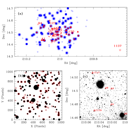
Figure 1: (a) Map of the stars on the Boötes I region. Stars with radial velocity measurements and identified as members, from Martin et al. (2007) are shown as filled red triangles. Koposov et al.’s (2011) sample is shown as open blue circles, and the stars having radial velocities consistent with the dSph are indicated as filled blue circles (74). In addition, the stars with velocities $95<V_{r}<108$ km/s are encircled by an outer blue ring (55), and those with a greater dispersion (19), but within the range $85<V_{r}<119$ km/s are the filled blue squares. The stars with high resolution spectroscopy discussed by Norris et al. (2009, 2010a, 2010b) and Feltzing et al. (2009) are numbered as Boo-1137 and Boo-127 as open red stars. The 7 RGB stars studied by Gilmore et al. (2013b) are indicated by red 5-point-line stars. The small red open circles are the 165 stars from HWB, and show the $4.78\times 4.78$ square-arcminute, APO SPIcam FOV. We also re-observed the outlying RGB stars in $vbyCT_{1}T_{2}(RI)$. (b) Finding chart for HWB’s data on a $1024\times 1024$ pixel scale. The black filled circles are proportional to $T_{1}$-magnitudes, and the open circles around them signify stars statistically likely to be Boo I members from color-comparisons. (c) The central field co-added image of the same field as (b), with the RGB stars from HWB and this paper identified.

Koposov et al. (2011) used an “enhanced” data reduction technique to achieve velocity errors of better than 1 km/s with the fiber-fed VLT/FLAMES+GIRAFFE system, around the $Ca{II}$-triplet (hereafter CaT, 8498, 8542, and 8662Å). Koposov et al.’s (2011) interpretation of their data prefers a two-component velocity distribution for Boötes I, with 98% confidence. We plot the finding chart for this survey, our photometric data and Martin et al.’s (2007) survey in Figure 1. Koposov et al. (2011) state that it is less likely that there is a one-component Gaussian with a velocity dispersion of $4.6^{+0.8}_{-0.6}$ km/s. About 70% of the stars in their data set have a velocity dispersion of $2.4^{+0.9}_{-0.7}$ km/s (the “colder” population) and a “hotter” population with a velocity dispersion of $~{}9$ km/s. They give an alternative explanation that Boötes I could have a one component velocity distribution, but that the stars’ velocities are not distributed isotropically; we agree with Koposov et al. (2011) that this model is hard to test without full spatial coverage. From Figure 1, it is clear that a much deeper survey needs to be made of the whole region out to at least 3 half-light radii, as Koposov et al. (2011) assert, but that there is likely to be a very low density of “halo” objects belonging to Boötes I. The multiple short exposures around CaT, used for the Koposov et al. (2011) study, can’t resolve metallicities below $[Fe/H]\sim-2.5$. High-resolution spectroscopy of these stars require about 15 hours observation each with VLT FLAMES and GIRAFFE and FLAMES (Gilmore et al., 2013a, b).

If we have any hope of mapping the full extent of Boötes I and examining the more distant systems which are likely to be found in the future, we need a more efficient method to identify age and metallicity spreads in sparsely populated systems, before selecting stars for spectroscopy. Martin et al. (2007) found only 30/96 stars identified as having the appropriate SDSS colors had Boötes I’s radial velocity. SDSS $ugriz$-filters were not designed for this task. In this paper, we are using the relatively well-studied Boötes I to find an efficient photometric method of locating dSph-members and solving for age and metallicity, with at least the $0.5~{}dex$ accuracy in $[Fe/H]$ given by the CaT spectra. Simply stated, our problem in studying the stellar populations in the dSphs/ultra-faint dwarfs (UFDs), is that some have few or no upper-red-giant branch stars. Without these bright stars, we require exposure-times of many thousands of seconds to achieve acceptable S/N, when observing in blue or UV filters. If we want to survey these objects spectroscopically, we should have an efficient way of identifying interesting stars by color, over and above the SDSS photometry. Traditional gravity-sensitive and metallicity-sensitive colours and indices involve the use of filters which become impractical with red, faint stars on the subgiant branch (SGB). Which blue filter is best for balancing metallicity sensitivity with achievable S/N? Our method for comparing spectroscopic and photometric metallicity measurements is set out in §2, with the observations described in §3. The detailed analysis is given in §4 and §5.

2 Method

How do we characterize the stellar populations of a system with similar properties to Boötes I? Studies show (Willman, 2010, and references therein) that the majority of these dSph and UFDs have very few red-giant branch (RGB) stars, which are normally the only stars bright enough for high-resolution spectroscopy.

2.1 Filters

We considered using some combination of the Washington, Strömgren, and SDSS filters, which are available at most observatories (see Figure 2). We began this project in 2007, imaging several of the dwarf galaxies using the Washington $CT_{1}T_{2}$-filters (using R & I instead of $T_{1}$ and $T_{2}$ to reduce observing time; see §2.3) in 2007, and the first paper on Boötes I has been published (HWB). The second, and concurrent, part of the imaging project began in early 2008, utilizing the Strömgren $vby$-filters. All the observations used for the analysis in this paper are given in Table 1, and discussed in detail in §3.

Our method used an evolving choice of filters, and the early part of the Strömgren work was described in Hughes & Wallerstein (2011a, b). Strong evidence of a spread in $[Fe/H]$ came from early spectroscopy (Martin et al., 2007), from our Washington observations (HWB), and higher resolution spectroscopy by Norris et al. (2008, 2010a, 2010b); Lai et al. (2011); Gilmore et al. (2013b).

The Washington system was used to define the Geisler & Sarajedini (1999, hereafter, GS99) standard giant branches. GS99 show that compared to Da Costa & Armandroff (1990), using the broad-band $V$- & $I$-filters, they can obtain three times the precision in metallicity determinations, at about a magnitude below the tip of the RGB, at around $M_{T_{1}}=-2.$

2.2 Metallicity Scales

Martin et al. (2007) and HWB found evidence of metallicity spread in Boötes I, which has been confirmed by higher resolution spectroscopy (Norris et al., 2008; Ivans, 2013 in preparation; Gilmore et al., 2013a, b). HWB’s estimate of the spread in $[Fe/H]$ for Boötes I was calibrated to GS99’s standard giant branches, and is therefore tied to the metallicity-scale of globular clusters used in that paper. Siegel (2006) notes that Boo I’s stellar population is similar to that of M92 as used in HWB, and we note that M92 and M15 are regarded as the most metal poor globular clusters at $[Fe/H]\sim-2.3$. GS99 discuss the metallicity scales of Zinn (1985); Zinn & West (1984); Carretta & Gratton (1997), and also define a “HDS” scale of their own, which takes the unweighted means of available high-dispersion spectroscopy (mostly from Rutledge, Hesser & Stetson’s (1997) study of calcium-triplet strengths). In GS99, the most metal-poor globular cluster in their study, M15, has $[Fe/H]=-2.24$ on the HDS scale, $[Fe/H]=-2.15$ on the Zinn & West (1984) scale, but -2.02 on the Carretta & Gratton (1997) calibration. Within the uncertainties, this magnitude of disagreement alone could explain the difference in mean [Fe/H] between the Washington photometry and the SDSS data (also see discussion in Hughes & Wallerstein, 2011a). The Washington filters and the GS99 standard giant branches are generally designed to return the CaT-matched metallicity scale of Zinn (1985). GS99 derive nine calibrations based on $M_{T_{1}}$ and metallicity, and let the user decide which is appropriate for their cluster/galaxy.

The HWB-average value of $[Fe/H]=-2.1^{+0.3}_{-0.5}$ dex was determined from the 7 brightest members of Boötes I in their data set (detected in the $CRI$ filters), with the smallest photometric uncertainties. Hughes & Wallerstein (2011a) discuss a recent paper by Lai et al. (2011) on Boötes I, which used low resolution spectra, the SDSS bands and other available filters to characterize the stars. Lai et al. (2011) determined [Fe/H], [C/Fe], and [$\alpha$/Fe] for each target star, utilizing a new version of the SEGUE Stellar Parameter Pipeline (SSPP; Lee et al., 2008a, b) named the n-SSPP (the method for non-SEGUE data). The Lai et al. (2011) study found the [Fe/H]-range to be about $2.0-2.5$ dex, and a mean $[Fe/H]=-2.59$ (with an uncertainty of $0.2$ dex in each measurement). HWB, using Washington photometry alone, find $[Fe/H]=-2.1$, and a range $>1.0$ dex in the central regions. Martin et al. (2007) studied 30 objects in Boötes I and found the same mean value as HWB with the calcium triplet (CaT) method. It is known that the CaT-calibration may skew to higher [Fe/H]-values at the lower-metallicity end, below $[Fe/H]\sim-2.0$ (Kirby et al., 2008). Koposov et al. (2011) comment that the inner regions of Boötes I do seem to be more metal-rich at the $2.4\sigma$ level, than the outer regions (Figure 1a), which our photometry does not cover. Koposov et al. (2011) examined 16 stars from Norris et al. (2010a) and showed that progressing radially outwards from the center of Figure 1a, the inner 8 stars have a mean $[Fe/H]=-2.30\pm 0.12$ and the outer 8 have $[Fe/H]=-2.78\pm 0.17$.

Frebel, Simon & Kirby (2011), have amassed a high-resolution spectroscopic study of the chemical composition of several UFDs, and a recent paper by Kirby et al. (2012) discusses how supernovae (SN) enrich/pollute the gas in low-mass dSphs. In the latter paper, they comment that SN in systems like Boötes I would be more effective at enrichment, on an individual basis, than early massive stars were at enriching the MW’s halo because there was less gas to contaminate. In addition, Kirby et al. (2012) note that a star in a dSph with $[Fe/H]\sim-3.0$ is sampling the previous generation of massive stars with $[Fe/H]<<-3.0$. This is a particularly important point when we consider that Norris et al. (2010b) have found that Boo-1137 has $[Fe/H]=-3.7$, and this is discussed at length in Gilmore et al. (2013a, b).

2.3 Practical Filter Sets for Studying Nearby Dwarf Galaxies

Hughes & Wallerstein (2011a, a summary of a conference presentation) discussed recent papers that explored the optimal colour-pairs to use for age and metallicity studies (e.g. Li & Han, 2008; Holtzman et al., 2011). However, much of the rhetoric is theoretical and involves testing on nearby, densely populated globular clusters. The search for practical colour-pairs also challenges the observer to use filters that can be employed on the same instrument, on the same night (if possible), to minimize zero-point offsets and seeing differences.

Ross et al. (2014) calibrated the Dartmouth isochrones for Hubble Space Telescope (HST)/Wide Field Camera 3 (WFC3) using 5 globular clusters in the metallicity range $-2.30<[Fe/H]<+0.4$. They found that clusters with known distances, reddening and ages could have their metallicities determined to $\sim 1.0$ dex (overall). Otherwise, non-pre-judged results on the globulars’ dominant metallicity showed the best colors to be: $F336W-F555W$ (SDSS-u combined with Johnson-V) yields the cluster metallicity to $\sim 0.2$ to $0.5$ dex (high to low metallicity), $F390M-F555W$ ($Ca_{II}$ Cont. combined with Johnson-V) gives $\sim 0.15$ to $0.25$ dex, and $F390W-F555W$ (Washington-C and Johnson-V) gives $\sim 0.2$ to $0.4$ dex. In this paper, we did not test $F390M$, but $(C-y)$ is equivalent to $(C-V)$. With the dSphs, the systems are not very well-studied, and we require the best color for individual stars, not the whole RGB.

Calamida et al. (2012) have produced a metallicity calibration for dwarf stars based on the Strömgren $m_{1}$-index and near-infrared colours, but their calibration works better for populations which are more metal-rich than the UFDs. In this section, we compare the various filter-combinations and note some pitfalls which may be unique to UFD populations. Figure 2a shows the transmission curves for the filters given in Table 2 (Bessell, 2005), taken from the CTIO website, with the ATLAS9 model flux density for a star with $T_{eff}=4750K$, $[Fe/H]=-2.5$, $[\alpha/Fe]=+0.4$, $\log g=1.5$.

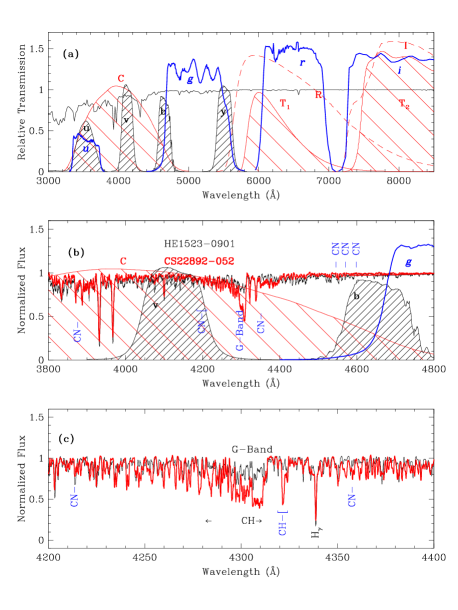
Figure 2: (a) Transmission curves for the filters given in Table 2, from the CTIO website. We also show the ATLAS9 model flux density for $T_{eff}=4750K$, $[Fe/H]=-2.5$, $[\alpha/Fe]=+0.4$, $\log g=1.5$. Strömgren filters (including $u$) are shown as shaded black curves. Washington filters are shown in shaded red, with the $R-$ and $I$-filters as dashed red lines. SDSS filters are shown in blue. (b) Normalized flux plots for HE1523-0901 (black) and CS22892-052 (red), from 3800-4800Å. We show the filter transmission curves for $C$ (red), $v$ (black), $b$ (black), and $g$ (blue) filters; we note the major CN and CH features. The original resolution has been smoothed to show the carbon-sensitive absorption. (c) The normalized flux curves for HE1523-0901 (black) and CS22892-052 (red), from 4200-4400Å, with major CN & CH spectral features marked.

Overall, the best photometric system designed for separating stars by metallicity is considered to be the intermediate-band Strömgren photometry (Strömgren, 1966). The distant RGB stars in the dSphs are very faint at Strömgren-u, and only the 8 brightest proper-motion members are detected at SDSS-u (6 from HWB and the 2 extra RGB stars with high-resolution spectra, including Boo-1137). Without the $u$-band, we are unable to obtain the surface gravity-sensitive, $c_{1}$-index, where

$$c_{1}=(u-v)-(v-b),$$ (1)

which measures the Balmer jump.

The metallicity of the stars ($Fe$ plus light elements) is sensitive to the $m_{1}$-index, where

$$m_{1}=(v-b)-(b-y).$$ (2)

The $(b-y)$-colour is a measure of the temperature and $(v-b)$ is a measure of metallic line blanketing (see Figure 2a). Many papers have mapped the Strömgren metallicity index to [Fe/H] (e.g Hilker, 2000; Calamida et al., 2007, 2009) and find that calibrations fail for the RGB stars at $(b-y)<0.5$ for all schemes. Faria et al. (2007) commented that the loci of metal-rich and metal-poor stars overlap on the lower-RGB, which they say is likely due to the larger photometric errors. Although this statement is not false, it is not the only reason for the issue (Figure 2). The $m_{1}$-index loses sensitivity as the difference in line absorption between $b$ and $v$ becomes equal to the difference in line absorption between $b$ and $y$ (Hughes & Wallerstein, 2011a). As stars become fainter lower down the RGB, the surface temperature rises and the lines get weaker (also see: Önehag et al., 2009; Árnadóttir, Feltzing & Lundström, 2010, and references therin). The latter paper discusses the VandenBerg, Bergbusch & Dowler (2006) isochrones and the temperature-colour transformation by Clem et al. (2004), and makes a point that their classification scheme can only be used for giants with $(b-y)_{0}\geq 0.6$.

Also from Figure 2, we can see the advantages that the Washington filters provide over the Strömgren and SDSS filters. The broad $C$-filter includes the metallicity-defining lines contained in the narrower $v$-filter and part of the $b$-filter, and also surface-gravity sensitive Strömgren-$u$ and SDSS-$u$. Thus, the colour $(C-T_{1})$ should be sensitive to $T_{eff}$, $[Fe/H]$, $[\alpha/Fe]$, and $\log g$ (GS99). The Strömgren filters are more effective than Washington bands in a system with a well-populated upper RGB, or if the stellar system is close enough to have $\sim 1$ per cent photometry below the sub-giant branch (SGB), where the isochrones separate. As discussed in HWB, Geisler (1996) and Geisler, Claria & Minniti (1991), the more-commonly used broadband $R-$ and $I$-filters can be converted linearly to Washington $T_{1}$ and $T_{2}$, but with less observing time needed (also see the filter profiles in Figure 2a). The $C$-filter is broader than the Johnson $B$-band, and is more sensitive to line-blanketing. Washington-$C$ is a better filter choice than Johnson-$B$ or Strömgren-$v$ for determining metallicity in faint, distant galaxies. Table 2 includes estimates for the total exposure times required to reach the main-sequence turn-off (MSTO) of dSphs with the WFPC3 on HST (also see Ross et al., 2014).

Summarizing comments by Sneden et al. (2003), metallicity is usually synonymous with [Fe/H], but other elements may be inhomogeneously-variable in dSphs as well as the Milky Way’s halo.

$$[Fe/H]=\log_{10}({N_{Fe}/N_{H}})_{*}-\log_{10}({N_{Fe}/N_{H}})_{\odot}.$$ (3)

The metallicity is normally taken to be:

$$Z=Z_{0}(0.694f_{\alpha}+0.306),$$ (4)

where $f_{\alpha}\equiv[\alpha/Fe]$, the $\alpha$-enhancement factor, and $Z_{0}$ is the “heavy element abundance by mass for the solar mixture with the same $[Fe/H]$” (Kim et al., 2002).

In Figure 2b and 2c, we use 2 metal-poor RGB stars to illustrate the sensitivity of the Strömgren, Washington and SDSS filters to carbon-enhancement. HE 1523-0901 (black line: Frebel et al., 2007) is a r-process-enhanced metal-poor star with $[Fe/H]\approx-3.0$, $[C/Fe]=-0.3$, $\log T_{eff}=4650K$, and $log\;g=1.0$. CS 22892-052 (red line) is also an r-process rich object (Sneden et al., 2003, 2009; Cowan et al., 2011) with $[Fe/H]\approx-3.0$, $[C/Fe]\approx 1.0$, $\log T_{eff}=4800K$, $log\;g=1.5$, and $[\alpha/Fe]\approx+0.3$. The change in the CH-caused G-band is apparent in Figure 2c, and CN/CH features affect the $C$ (in particular), $v-$, and $b$-filters, but the SDSS $g$-band is relatively clear of contamination, but $g$ is not very sensitive to metallicity either. The spectra shown in Figure 2 were provided by Anna Frebel (private communication).

Carretta et al. (2011) reports a study of globular cluster stars with CN/CH variations. They discuss other ways to construct Strömgren-indices, finding a filter combination that will separate the first and second generations of globular cluster stars. Carretta et al. (2011) settled on

$$c_{y}=c_{1}-(b-y)$$ (5)

$$\delta_{4}=(u-v)-(b-y),$$ (6)

with $c_{y}$ being defined by Yong et al. (2008), and is an index which is sensitive to gravity and $N$. Both of these indices have limited use in our study, since they require high precision photometry at the Strömgren-$u-$ and $v-$bands. Carretta et al. (2011) point out that $m_{1}$ and $c_{y}$ have a “complicated,” degenerate dependence on metallicity (involving $[Fe/H]$ and $N$), and show that $\delta_{4}$ is much more effective at estimating the $N-$abundance, and remains $CNO$-sensitive over a much broader range of stellar temperatures, metallicities and surface gravities, since the temperature dependence is weak. Carretta et al. (2011) are more concerned with separating the N-poor, Na-poor, O-rich first generation globular population, from the N-rich, Na-rich, O-poor, second generation stars (if present). We note that there is a particular problem which involves the carbon-rich stars in the dSphs, because their colours always make a metal-poor star mimic those of a much more metal-rich object.

3 Observations

As in HWB, we observed the same central field (see Table 1) in Boötes I ($RA=14^{h}00^{m}06^{s},Dec=14.5^{\circ}$ J2000) with the Apache Point Observatory’s 3.5-m telescope, using the direct imaging SPIcam system. The detector is a backside-illuminated SITe TK2048E $2048\times 2048$ pixel CCD with 24 micron pixels, which we binned ($2\times 2$), giving a plate scale of 0.28 arc seconds per pixel, and a field of view (FOV) of $4.78\times 4.78$ square arcminutes. The HWB data set for Boötes I was taken on 2007 March 19 (with a comparison field in M92 taken on 2007 May 24). We took 21 frames in Washington C, and Cousins R and I filters, with exposure time ranging from 1 seconds to 1000 seconds. The readout noise was 5.7e- with a gain of 3.4 e-/ADU. The images were flat-fielded using dome or night-sky flats, along with with a sequence of zeros. We then processed the frames using the image-processing software in IRAF.

The $vby$-observations used in this paper are detailed in Table 1, along with the Washington filter data from HWB (when the seeing, and most airmass-values, were noticeably better). The Strömgren data was taken on 2009 January 17-18, 2009 May 1, and 2011 April 5. The January 2009 data used the $2\times 2\;in^{2}$ Strömgren filter set, which had vignetted the images. The 3-inch square $uvby$ filters arrived from the manufacturer (Custom Scientific, Inc., of Pheonix, AZ) after the January 2009 observing run. We compared the Boötes I stars observed in January and May 2009 and found that there was no appreciable difference in the instrumental magnitudes at the same airmass. The photometric quality of the January data was better than the May data, but the January 2009 images were taken with the smaller filters. After some questions about recorded exposure times in the image headers were resolved, more frames were taken in April, 2011, to ensure stability of the zero-points. We also took some additional images in June, 2012 in $C$ and $R$, but the seeing was never better than $1.5\arcsec$ so they are not included. The final weighted mean-magnitude program rejected the latter observations because of poor image quality compared to the earlier frames. In addition to the Boötes I central field chosen in 2007, we also observed two RGB stars, in separate fields, which had high resolution spectra in the literature: Boo-1137 and Boo-127 (Norris et al., 2010a, b; Frebel, Kirby & Simon, 2010; Feltzing et al., 2009).

Table 1 lists the data taken at APO. The images taken on 2007 March 19 had sub-arcsecond seeing, and enabled us to make the best possible master source list for DAOPHOT. For conversion to the standard Washington system, we used the Geisler (1996) Washington standard frames, containing at least 5 stars in each frame, for at least 30 standards per half-night (the APO 3.5-m is scheduled in that manner). For the Strömgren data, this was more of an issue, since the Strömgren system was calibrated with single stars. To reduce observing overheads, we used M92 as a cluster standard. We used the M92 fiducial lines to assist in matching the APO data to the standard system. To supplement the HWB Washington data, we took $C$ and $R$ images of the Boötes I central field in 2009 (not $I$), to make sure that there was no calibration issue with the earlier data. No problems were detected.

Employing the same data reduction method as HWB, we used two iterations of (DAOPHOT-PHOT-ALLSTAR), with the first iteration having a detection threshold of 4$\sigma$, and the second pass had a 5$\sigma$ detection limit. We used $\sim 10$ stars in each frame to construct the point spread functions (PSFs), and assume that it do not vary over the chip. The chip had been found to be very stable and there has been no evidence that the PSF varies over the image. ALLSTAR (Stetson, 1987) was further constrained to only detect objects with a CHI-value $<2.0$, and almost all sources had CHI (the DAOPHOT goodness-of-fit statistic) between 0.5 and 1.5 (to remove cosmic rays and non-stellar, extended objects). We found the aperture correction between the small (4 pixel) aperture used by ALLSTAR in the Boötes I field, and the larger (10-15 pixel) aperture used for the standards, by using the best point spread function (PSF) stars in each images. We used the IMMATCH task to match the sources in each image, making several datasets in each filter combination. We then put together the final source list as follows: requiring that each star be detected in at east one image in each filter, and the final magnitude and colours were calculated as the weighted (airmass, FWHM, DAOPHOT uncertainty) mean of each individual detection.

We later tested the final photometry using the standalone version of ALLFRAME (Stetson, 1994), and found that the results were consistent with our method. When we used DAOPHOT III/ALLFRAME, this method produced almost identical results to those obtained by manually shifting all the images to the same positions, median-filtering them all and producing a source list from that. When we used that master-list to feed into the IRAF version of ALLSTAR, it produced 166 total detections seen at $vbyCT_{1}T_{2}(RI)$, but the v-band data is noticeably noisier, as expected. Compared to the HWB list, 117 objects were detected, and we use this group of objects in the comparison to M92. We find that there are 34 objects having a $v$-band uncertainty less than 0.10 dex, which were detected in multiple frames in each band (on more than one night), and had a lower overall standard-deviation-of-the-mean uncertainty; these objects are listed in Table 3. However, we plot the full-dataset in Figure 3, to show the uncertainty in magnitudes and colors, for comparison with models in §6.

In order to display how well DAOPHOT (both versions) worked on the central Boötes I field, we used the median-filtered images in each filter to show the uncertainty for each object against $T_{1}$ and $V(y)$. This is the best measure of how well DAOPHOT is working, and it is correlated with airmass and seeing. The images are not crowded, we have a factor of 10 fewer objets than we would detect in M92. With the artificial star experiments, the completeness of the data set is controlled by the $v$-band magnitude. The only completeness issue involves the 2 bright foreground stars seen in Figure 1c, but the source density is too low for many objects to be missed. At this point, we are not constructing luminosity functions below the MSTO, so completeness is less of a concern than the photometric uncertainties for each star. Using M92 as a cluster standard, we reduced the frames using IRAF’s DAOPHOT, with 20-30 stars to fit the PSF. We then selected stars on the outer parts of the globular cluster for testing; our photometry yielded matches to the standard system used for $\sim 20$ randomly selected stars in common with the Frank Grundahl M92’s data set private communication, F. Grundahl; Grundahl et al. 2000 of $\sigma_{rms}=0.026$ in $V(y)$, $\sigma_{rms}=0.035$ in $(b-y)$, and $\sigma_{rms}=0.046$ in $m_{1}$. Our confirmation frames from 2011 were only deep enough to detect the bright RGB stars in Boötes I, so those stars have more observations and hence lower uncertainties in $vbyCT_{1}$. In Figure 4, we show colour-magnitude diagrams used for calibration of Boo I to M92 (cyan points: Grundahl et al., 2000). The dark blue line is the Dartmouth isochrone (Dotter et al., 2008) which fits well with a recent study by di Cecco et al. (2010), $DM=14.74$, $[Fe/H]=-2.32$, $[\alpha/Fe]=0.3$ and $Y=0.248$, and Age$=11\pm 1.5$ Gyr. Boötes I is taken to have $E(B-V)=0.02$ and $DM=19.11$, as used in HWB.

Table 1: APO 3.5-m CCD Frames taken in 2007-2011

Field	UT1	Filter	$\tau(s)$	Airmass2	FWHM(′′)3
Boo-127	09-01-18	y	300	1.19	1.0
Boo-127	09-01-18	b	600	1.17	1.8
Boo-127	09-01-18	v	1200	1.14	1.6
Boo-1137	09-01-18	y	300	1.10	1.0
Boo-1137	09-01-18	b	600	1.09	1.3
Boo-1137	09-01-18	v	1200	1.08	0.9
Boo Ic4	09-05-01	b	1500	1.25	0.9
Boo Ic	09-05-01	y	900	1.33	1.0
Boo Ic	09-05-01	y	600	1.87	1.0
Boo Ic	09-05-01	b	900	1.65	1.0
Boo Ic	09-05-01	b	900	2.06	1.2
Boo Ic	09-05-01	v	1200	2.35	1.3
Boo Ic	09-05-01	v	2100	1.48	1.0
Boo Ic	11-04-05	R	300	1.08	0.9
Boo Ic	11-04-05	C	900	1.07	1.3
Boo Ic	11-04-05	y	600	1.06	1.1
Boo Ic	11-04-05	b	600	1.06	1.1
Boo Ic	11-04-05	v	1200	1.05	1.3
Boo-1137	11-04-05	R	300	1.08	1.3
Boo-1137	11-04-05	C	900	1.09	1.4
Boo-1137	11-04-05	y	600	1.11	1.5
Boo-1137	11-04-05	b	800	1.13	0.9
Boo-1137	11-04-05	v	1200	1.16	1.0
Boo-127	11-04-05	R	300	1.22	1.1
Boo-127	11-04-05	C	900	1.24	1.5
Boo-127	11-04-05	y	600	1.30	1.3
Boo-127	11-04-05	b	800	1.34	1.2
Boo-127	11-04-05	v	1200	1.40	1.7
Boo Ic	07-03-19	R	1	1.07	0.9
Boo Ic	07-03-19	R	3	1.07	0.8
Boo Ic	07-03-19	R	10	1.06	0.8
Boo Ic	07-03-19	R	30	1.06	0.8
Boo Ic	07-03-19	R	90	1.06	0.8
Boo Ic	07-03-19	R	300	1.06	0.7
Boo Ic	07-03-19	R	1000	1.06	0.8
Boo Ic	07-03-19	I	1	1.05	0.6
Boo Ic	07-03-19	I	3	1.05	0.6
Boo Ic	07-03-19	I	10	1.05	0.6
Boo Ic	07-03-19	I	30	1.05	0.6
Boo Ic	07-03-19	I	90	1.05	0.7
Boo Ic	07-03-19	I	300	1.05	0.7
Boo Ic	07-03-19	I	1000	1.05	0.8
Boo Ic	07-03-19	C	1	1.06	0.7
Boo Ic	07-03-19	C	3	1.06	0.9
Boo Ic	07-03-19	C	10	1.06	0.8
Boo Ic	07-03-19	C	30	1.06	0.7
Boo Ic	07-03-19	C	90	1.06	0.8
Boo Ic	07-03-19	C	300	1.07	0.7
Boo Ic	07-03-19	C	1000	1.07	0.7

(1) Year-Month-Day

(2) Effective airmass

(3) Average seeing

(4) Boo Ic:- Boötes I central field, see Figure 1c.

Table 2: Filters Considered

Filter1	$\lambda$(Å)	$\Delta\lambda$(Å)	System	HST/WFC32	$\tau(s)^{3}$
u	3520	314	Strömgren	F390M	18,980
v	4100	170	Strömgren	F410M	10,214
b	4688	185	Strömgren	F461M	5318
y	5480	226	Strömgren	F547M	1,494
C	3980	1100	Washington	F390W	2,612
$T_{1}$	6389	770	Use $R_{C}$	F625W	605
$T_{2}$	8051	1420	Use $I_{C}$	F775W	390
$R$	6407	1580	Use $R_{C}$	F625W	605
$I$	7980	1540	Use $I_{C}$	F775W	390
u	3596	570	SDSS	F336W	6,336
g	4639	1280	SDSS	F475W	835
r	6122	1150	SDSS	F625W	605
i	7439	1230	SDSS	F775W	988

(1) Filter data from Bessell (2005).

(2) HST/WFC3 filter best equivalent to ground-based choice.

(3) Estimated exposure time for a G2V star at $V\sim 23$ mag. at the distance of Boötes I for $S/N=50$.

We solved for each filter, rather than the Strömgren indices, for each night. The transformation equations on 2009 May 1 are as follows:

$$V=y_{i}-2.187-0.012(b_{i}-y_{i})-0.163X,\;\sigma_{rms}=0.007$$ (7)

$$b=b_{i}-2.217+0.031(b_{i}-y_{i})+0.220X,\;\sigma_{rms}=0.017$$ (8)

$$v=v_{i}-2.464-0.512(v_{i}-b_{i})-0.300X,\;\sigma_{rms}=0.020$$ (9)

Here, X denotes the effective airmass and the subscript i indicates the instrumental magnitude. The $\sigma_{rms}$ values are the comparison with the standards.

HWB’s photometry from 2007 March 19 yielded matches to the GS99 standard system of $\sigma_{rms}=0.021$ in $T_{1}$, $\sigma_{rms}=0.015$ in $(C-T_{1})$, and $\sigma_{rms}=0.017$ in $(T_{1}-T_{2})$. In $T_{1}$, the average uncertainties in the final CMD were $\sigma_{rms}=0.024$ at the level of the horizontal branch, and $\sigma_{rms}=0.04$ at the MSTO. The transformation equations are as follows:

$$T_{1}=R_{i}-0.461+0.021(C_{i}-R_{i})-0.150X,\;\sigma_{rms}=0.021$$ (10)

$$(C-T_{1})=1.117(C_{i}-R_{i})-1.015-0.322X,\;\sigma_{rms}=0.015$$ (11)

$$(T_{1}-T_{2})=1.058(R_{i}-I_{i})+0.460-0.046X,\;\sigma_{rms}=0.017$$ (12)

As before, X denotes the airmass and the subscript i indicates the instrumental magnitude.

The final calculated uncertainties for each individual star in each image were found by taking the uncertainties from photon statistics, DAOPHOT’s uncertainties, the aperture corrections, and the standard photometric errors in quadrature. We then took the weighted means of multiple observations, which reduced uncertainties internal to the data set. Thus, we achieved better uncertainties in for each star by taking the weighted means, with the weighting being dependent on the DAOPHOT uncertainties and the airmass, which was found to be equivalent to the seeing. We constructed image sets comparing short and long exposures, keeping to similar airmass and seeing between frames, to achieve multiple, independent observations of each star and improved the final (standard-deviation-of-the-mean) uncertainty for the objects above $T_{1}\sim 22~{}mag.$ We were able to detect 166 objects in the field in the $vbyCT_{1}T_{2}(RI)$-filters. A finding chart for the objects in Table 3 (117 objects) is given in HWB, and is shown in Figure 1b and 1c here. Also, from Table 3, the 19 brightest stars were detected in the SDSS survey, and we include them in Table 4.

An independent, external test on how well we have calibrated the data is discussed in §6.1, which covers spectral energy distributions (SEDs).

4 STATISTICAL REMOVAL OF NON-MEMBERS

The process used by HWB to remove non-dSph stars from our final data set was modified from that used on the globular clusters, NGC 6388 and $\omega$ Cen (Hughes et al., 2007; Hughes & Wallerstein, 2000, respectively). Due to observing-time constraints, we did not observe an off-galaxy field, but instead generated artificial field stars with the TRILEGAL code (Girardi et al., 2005), calibrated for the SPIcam FOV and the appropriate magnitude limits. Briefly, we can statistically compare CMD of the off-galaxy region (or the simulated field) to the Boötes I field. The method was adapted from Mighell, Sarajedini & French (1998). Here, we detail the method used to remove foreground objects from the HWB data set, which was also used with the Strömgren for consistency, yielding similar results. The meaning of the letter grades in Table 3 is as follows. Class A are sources which have passed statistical cleaning and colour-selection, and which have uncertainties better than 0.05 in all Washington filters. Class B are sources which have passed statistical cleaning and colour-selection, which do not have uncertainties better than 0.05 in all filters. Class C are sources which passed colour-selection failed statistical cleaning, and which have uncertainties better than 0.05 in all filters. Class D objects passed colour-selection, failed statistical cleaning, and do not have uncertainties better than 0.05 in all filters. Class E sources passed statistical cleaning but failed colour selection, and Class F failed statistical cleaning and colour selection. Where the whole image is filled by the target (galaxy or globular cluster), we would have to use an off-target field (or simulate one). For each star in the on-target image sub-section (or separate image), we count the number of stars in the colour-magnitude diagram that have $C$-magnitudes (HWB) within max (2.0, 0.2) mag. of the $C$ and $C-T_{1}$ colours of the supposed dwarf-population stars in the CMD. We call this number $N_{on}$. Now, we also count the number of field stars, in the off-dwarf image or image sub-section (or simulated field), that fall within the same ranges in the CMD, and call this number $N_{off}$.

We calculate the probability that the star in the on-dwarf field CMD is a member of the dwarf galaxy population as:

$$p\approx 1-min\left({\alpha N_{off}^{UL\;84}\over N_{on}^{LL\;95}},\;1.0\right)$$ (13)

Where $\alpha$ is the ratio of the area of the dSph galaxy region to the area of the (simulated) field region and

$$N_{off}^{UL\;84}\approx\\ (N_{off}+1)\left[1-{1\over 9(N_{off}+1)}+{1.000\over 3\sqrt{N_{off}+1}}\right]^{3}$$ (14)

The equations are taken from the Appendix of Hughes & Wallerstein (2000), and corresponding to eq. [2] of Mighell, Sarajedini & French (1998) and eq. [9] of Gehrels (1986). Here, eq.[14] is the estimated upper (84 per cent ) confidence limit of $N_{off}$, using Gaussian statistics.

$$N_{on}^{LL\;95}\approx\\ N_{on}\times\left[1-{1\over 9N_{on}}-{1.645\over 3\sqrt{N_{on}}}+0.031N_{on}^{-2.50}\right]^{3}$$ (15)

Then, eq.[15] is then the lower 95 per cent confidence limit for $N_{on}$ (eq. [3] of Mighell, Sarajedini & French (1998), and eq. [14] of Gehrels (1986)). For a large, relatively nearby cluster like $\omega$ Cen, we assumed that the whole on-cluster field is part of the system (a fairly safe assumption), so that $\alpha$ is assumed to be 1, in that case. Here, we generated a population of MWG stars with the TRILEGAL code for the same sky area as the SPIcam FOV, so that $\alpha=1$ for Boötes I, also. Then, in order to estimate if any particular star is a cluster/dwarf member, we generate a uniform random number, $0<p^{\prime}<1$, and if (eq.[13]’s) $p>p^{\prime}$, we accept the star as a member of the cluster or dwarf galaxy. This method works best if there is a colour/metallicity difference between the foreground and Boötes I dwarf populations, which means it is less effective at removing field stars if we use the SDSS-filters.

Figure 3a–c shows the final photometric uncertainties from the Washington filter data. We re-reduced the data, and made a median-filtered images for each $vbyCT_{1}T_{2}(RI)$-filter, shifted the images, and made a master list of objected detected in a summed master-median-filtered image. The open circles are the 166 objects detected in all the median-filters images. Figure 3d–f shows the uncertainty distribution for the 166 detections in the $vby$-filters as open circles. The Washington-filter images had fainter magnitude limits than the Strömgren images, so we continue to use the statistical cleaning results from HWB, but we can use the Strömgren indices to estimate photometric metallicities and compare with the statistical results. Observing time in the v-filter is controlling our limiting magnitude. We compared the 166 objects detected in the median-filtered images in all 6 bands, compared them with the 165 objects from HWB, and 117 objects passed the DAOPHOT CHI-value $<2.0$ in the $v$-band, and we merged the two lists. Table 3 contains the 34 objects which were observed on more than one night in all filters and had uncertainties $<0.1$ in the $v$-band. The analysis from this point onwards requires that all objects have at least $vbyCT_{1}$-magnitudes.

Table 3: Objects in Boötes I with Washington & Strömgren Photometry

ID1	$X_{R}^{2}$	$Y_{R}$	RA	DEC	Class3	$T_{1}$	$(C-T_{1})$	$(T_{1}-T_{2})$	$V$	$(b-y)$	$m_{1}$
Boo-1137	$-$	$-$	13:58:33.82	14:21:08.5	A	17.08(0.02)	1.69(0.03)	0.61(0.02)	17.65(0.01)	0.62(0.02)	0.09(0.03)
Boo-127	$-$	$-$	14:00:14.57	14:35:52.1	A	17.12(0.02)	1.84(0.03)	0.57(0.02)	17.68(0.004)	0.68(0.02)	0.14(0.03)
Boo-117/HWB-8	298.68	891.95	14:00:10.49	14:31:45.6	C	17.20(0.02)	1.82(0.03)	0.61(0.02)	17.79(0.004)	0.61(0.02)	0.16(0.03)
Boo-119/HWB-9	330.67	171.27	14:00:09.85	14:28:23.1	A	17.48(0.02)	1.80(0.03)	0.57(0.02)	17.98(0.005)	0.63(0.02)	0.20(0.03)
HWB-22	950.94	97.89	13:59:57.85	14:28:02.8	A	19.77(0.02)	1.16(0.04)	0.47(0.02)	20.22(0.01)	0.47(0.02)	0.04(0.04)
HWB-24	667.94	272.14	14:00:03.33	14:28:51.6	C	20.10(0.02)	1.06(0.03)	0.50(0.02)	20.48(0.01)	0.42(0.03)	0.04(0.06)
HWB-28	564.80	599.22	14:00:05.34	14:30:23.5	A	20.40(0.02)	1.16(0.04)	0.50(0.03)	20.88(0.02)	0.45(0.03)	0.09(0.04)
HWB-34	681.50	600.22	14:00:03.08	14:30:23.8	A	20.86(0.02)	1.09(0.04)	0.46(0.02)	21.27(0.02)	0.44(0.04)	0.03(0.06)
HWB-3	960.10	499.42	13:59:57.69	14:29:55.6	F	16.01(0.01)	3.47(0.03)	1.65(0.03)	16.91(0.03)	1.27(0.03)	-0.03(0.04)
HWB-4	54.57	53.07	14:00:15.18	14:27:49.8	F	16.24(0.01)	3.29(0.03)	1.28(0.03)	17.17(0.02)	1.02(0.03)	0.33(0.05)
HWB-6	630.81	818.25	14:00:04.07	14:31:25.1	E	16.86(0.01)	1.20(0.03)	0.49(0.02)	17.26(0.02)	0.44(0.03)	0.08(0.05)
HWB-11	891.80	840.98	13:59:59.02	14:31:31.5	E	17.71(0.01)	3.26(0.03)	1.10(0.02)	18.67(0.01)	0.97(0.02)	0.46(0.04)
HWB-14	540.96	301.43	14:00:05.78	14:28:59.8	E	18.63(0.01)	0.96(0.03)	0.40(0.02)	18.95(0.02)	0.40(0.03)	0.09(0.05)
HWB-15	461.31	912.01	14:00:07.35	14:31:51.3	E	18.79(0.01)	3.39(0.03)	1.30(0.02)	19.82(0.02)	1.04(0.03)	0.37(0.06)
HWB-16	287.26	389.96	14:00:10.69	14:29:24.6	A	18.92(0.01)	1.37(0.03)	0.52(0.02)	19.39(0.02)	0.52(0.03)	0.07(0.04)
HWB-17	72.98	337.39	14:00:14.84	14:29:09.7	F	19.06(0.01)	0.88(0.03)	0.38(0.02)	19.40(0.01)	0.35(0.02)	0.08(0.04)
HWB-18	171.21	684.41	14:00:12.95	14:30:47.3	E	19.23(0.01)	2.11(0.03)	0.59(0.02)	19.83(0.01)	0.59(0.02)	0.46(0.04)
HWB-19	626.80	6.28	14:00:04.11	14:27:36.9	A	19.33(0.02)	0.87(0.03)	0.38(0.02)	19.59(0.01)	0.36(0.03)	0.07(0.04)
HWB-20	329.81	701.76	14:00:09.88	14:30:52.2	E	19.37(0.01)	2.73(0.03)	0.86(0.02)	20.18(0.02)	0.80(0.04)	0.51(0.06)
HWB-21	963.85	2.41	13:59:57.59	14:27:35.9	E	19.57(0.01)	3.12(0.06)	0.94(0.02)	20.38(0.02)	0.96(0.03)	0.32(0.09)
HWB-26	589.61	886.86	14:00:04.87	14:31:44.3	E	20.30(0.02)	2.78(0.04)	0.88(0.02)	21.13(0.02)	0.77(0.04)	0.59(0.07)
HWB-29	510.88	714.46	14:00:06.38	14:30:55.8	A	20.47(0.01)	1.20(0.03)	0.63(0.03)	20.91(0.02)	0.46(0.03)	0.08(0.07)
HWB-31	207.93	381.42	14:00:12.23	14:29:22.1	C	20.72(0.01)	0.97(0.03)	0.46(0.03)	21.09(0.02)	0.44(0.03)	-0.04(0.04)
HWB-32	692.68	332.82	14:00:02.85	14:29:08.7	E	20.77(0.01)	0.76(0.03)	0.36(0.02)	20.99(0.03)	0.32(0.03)	0.03(0.05)
HWB-33	848.41	14.94	13:59:59.83	14:27:39.4	E	20.84(0.01)	0.96(0.04)	0.36(0.03)	21.14(0.02)	0.44(0.03)	-0.04(0.05)
HWB-36	653.27	903.42	14:00:03.64	14:31:49.0	E	20.95(0.02)	1.12(0.04)	0.41(0.03)	21.40(0.03)	0.44(0.04)	0.01(0.06)
HWB-37	925.81	867.63	13:59:58.36	14:31:39.0	E	21.06(0.01)	1.80(0.05)	0.59(0.02)	21.60(0.03)	0.52(0.05)	0.31(0.08)
HWB-40	789.33	824.54	14:00:01.00	14:31:26.9	A	21.28(0.02)	1.13(0.04)	0.50(0.03)	21.64(0.03)	0.46(0.04)	0.05(0.07)
HWB-44	945.51	434.38	13:59:57.97	14:29:37.3	E	21.52(0.02)	1.00(0.04)	0.39(0.03)	21.86(0.04)	0.43(0.05)	-0.06(0.08)
HWB-45	545.05	475.10	14:00:05.71	14:29:48.6	A	21.54(0.01)	0.21(0.03)	0.57(0.03)	22.03(0.04)	0.34(0.05)	-1.02(0.07)
HWB-47	673.78	935.68	14:00:03.24	14:31:58.1	A	21.75(0.02)	0.92(0.04)	0.47(0.04)	22.11(0.04)	0.36(0.06)	0.10(0.09)
HWB-48	845.80	760.07	13:59:59.91	14:31:08.8	A	21.82(0.02)	-0.08(0.04)	0.17(0.05)	21.78(0.03)	0.07(0.05)	0.08(0.06)
HWB-50	87.95	538.21	14:00:14.56	14:30:06.1	A	21.92(0.02)	0.86(0.05)	0.40(0.03)	22.28(0.05)	0.38(0.07)	0.02(0.09)
HWB-51	661.84	801.67	14:00:03.47	14:31:20.4	A	21.92(0.02)	0.33(0.04)	0.28(0.05)	22.05(0.05)	0.24(0.06)	0.05(0.08)

(1) $ID$ from HWB, proper motion-confirmed members listed first.

(2) Positions from the Figure 1b.

(3) HWB’s object classes:

A - If sources passed the statistical cleaning process, had the correct colours and had photometry in all filters with uncertainties less than 0.05.

B - Objects passed the cleaning program, but had uncertainties in all filters not less than 0.05.

C - Passed the statistical cleaning process, had the correct colours and A-type good photometry, but failed the comparison with the randomly generated probability.

D - Objects failed the statistical cleaning process (also had the right colours but poor photometry).

E - Passed statistical cleaning but failed colour selection (according to HWB, ).

F - These objects failed both statistical cleaning and colour selection, and tended to be well outside the CMD area of a metal-poor dwarf. Usually bright foreground stars.

Figure 3: Uncertainty vs. magnitude plots for the Boo I data sets, from HWB and this paper. Open circles are 166 stars with $CT_{1}T_{2}$-measurements. These are the DAOPHOT uncertainties from the master-median-filtered images in each of the 6 filters. (a) Uncertainty in $T_{1}$ vs. $T_{1}$. (b) Uncertainty in $(C-T_{1})$ vs. $T_{1}$. (c) Uncertainty in $(T_{1}-T_{2})$ vs. $T_{1}$. (d) Uncertainty in $V_{y}$ vs. $V_{y}$, which is Johnson-$V$ calculated from Strömgren-$y$. (e) Uncertainty in $(b-y)$ vs. $V_{y}$. (f) Uncertainty in $m_{1}$ vs. $V_{y}$.

5 Photometric Metallicities

Following on from the discussion in §2, several authors have generated photometric calibrations on the Strömgren [Fe/H]-scale, amongst them, Hilker (2000) and Calamida et al. (2007). In this section, we select several calibrations from those papers, where $m_{0}$ is the dereddened $m_{1}$-index and $[m]$ is the reddening-free version:

$$Hilker\;(2000)\;:\;\\ [Fe/H]_{Hil}={m_{0}-1.277(b-y)_{0}+0.331\over 0.324(b-y)_{0}-0.031}.$$ (16)

$$Calamida\;et\;al.\;(2007):\;\\ [Fe/H]_{m_{1}}={m_{0}+0.309-0.521(v-y)_{0}\over 0.159(v-y)_{0}-0.090}.$$ (17)

$$Calamida\;et\;al.\;(2007):\;\\ [Fe/H]_{[m]}={[m]+0.251-0.585(v-y)_{0}\over 0.131(v-y)_{0}-0.070}.$$ (18)

These methods of calculating photometric metallicities are used for columns 2–4 of Table 5.

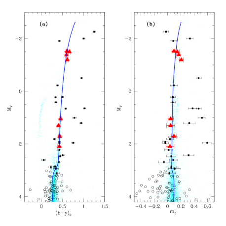
Figure 4: (a) $M_{V}\;vs.\;(b-y)_{0}$ Strömgren CMD for M92 (cyan points; data provided by F. Grundahl), Boo I Strömgren data only (black points), Strömgren and Washington objects (black filled circles), and proper-motion members with Strömgren, Washington and SDSS magnitudes (red filled triangles). The dark blue line is the Dartmouth isochrone corresponding to $[Fe/H]=-2.25$, $[\alpha/Fe]=0.3$ and an age of 11 Gyr. M92 has $E(B-V)=0.025$ and $DM=14.74$. Boo I has $E(B-V)=0.02$ and $DM=19.11$. (b) $M_{V}\;vs.\;m_{0}$, the Strömgren CMD for M92 (cyan points), Boo I Strömgren data only (black points), Strömgren and Washington objects (black filled circles), and proper-motion members with Strömgren, Washington and SDSS magnitudes (red filled triangles). The dark blue line is the Dartmouth isochrone corresponding to $[Fe/H]=-2.25$, $[\alpha/Fe]=+0.3$, and an age of 11.0 Gyr.

In Figure 5a and 5b, we show colour-colour plots and [Fe/H]-calibrations for M92 (cyan points). The blue points are the M92 RGB stars above the horizontal branch (HB). Having the same type of cool, metal-poor RGB as the expected dSph population, these plots illustrate the loss of metallicity resolution on the lower-RGB in the Strömgren system. We used the TRILEGAL code to generate a field of artificial stars at the correct galactic latitude, for the same magnitude limits as our dSph field. Figure 5c and 5d show our Boötes I data from Table 3 (black points with error bars) and the TRILEGAL-generated artificial stars (blue circles). The red triangles are the bright RGB stars with SDSS-colours. The Strömgren filters are well-suited to separate the dSph population from the foreground stars. We note that the TRILEGAL artificial stars have the same colors as the foreground RGB stars, and are separate from the upper-RGB proper-motion members Figure 5c and 5d; all data points overlap for stars which likely have $\log~{}g>2.5$, which is not a function of photometric uncertainty, it is the Strömgren bands losing sensitivity to metallicity. We confirm that the Strömgren  indices are only useful for upper RGB stars from these plots alone.

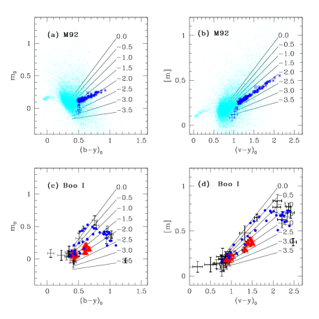
Figure 5: (a) Plot of $m_{0}=(v-b)_{0}-(b-y)_{0}$ vs. $(b-y)_{0}$ for M92 RGB stars (blue points, F.Grundahl, private communication), and the rest of the globular cluster’s stars (cyan). The calibration lines of constant [Fe/H] are taken from Hilker (2000). (b) For the same M92 sample, we show $[m]=m_{1}+0.3(b-y)$, the reddening-free index, plotted against $(v-y)_{0}$. Calibration from Calamida et al. (2007). (c) $m_{0}=(v-b)_{0}-(b-y)_{0}$ vs. $(b-y)_{0}$ for our sample (from the median filtered images), with the Hilker (2000) calibration. In total, 117 objects were detected in $vby$ filters, shown as black points. The TRILEGAL code was used to generate a sample of foreground stars, shown as blue filled circles. The RGB proper-motion members are shown as red triangles. (d) $[m]=m_{1}+0.3(b-y)\;vs.\;(v-y)_{0}$ for the same sample of Boötes I stars, with the Calamida et al. (2007) calibration.

We use the usual Strömgren relationships:

$$E(b-y) =0.70E(B-V);$$ (19)

$$E(v-y) =1.33E(B-V);$$ (20)

$$E(m_{1}) =-0.30E(b-y);$$ (21)

$${[m]} =m_{1}+0.30(b-y).$$ (22)

The reddening-free metallicity index is $[m]$, as used by Calamida et al. (2007); the reddening law is taken from Cardelli, Clayton & Mathis (1989) and Crawford (1975).

Calamida et al. (2007) generated several versions of the Strömgren-$[Fe/H]$ calibration, which we tested with our Table 3 data; their calibration equations that best fit our data are given in equations [17] & [18]. These calibrations were chosen because they best matched the spectroscopy available in 2010 (Feltzing et al., 2009; Norris et al., 2008; Ivans, 2009; Martin et al., 2007). The Calamida et al. (2007) equations are based on “semiempirical” calibrations of Clem et al. (2004), and have differences between the $[Fe/H]_{phot}$ and $[Fe/H]_{spec}$ values of $-0.06\pm 0.18$ dex and $-0.05\pm 0.18$ dex, respectively.

When Calamida et al. (2007) tested the Hilker (2000) calibration on 73 field RGB stars, the difference between the schemes was found to be $0.13\pm 0.20$ dex. Hughes et al. (2004) used the Hilker (2000) calibration for their study of $\omega$ Cen, which Calamida et al. (2009) found to be in agreement with their work. For stellar populations in dSph galaxies, it is impractical to use any calibration involving the $u$-band, both because the RGB and MS stars are too faint in the near-UV, but Strömgren-$u$ is more sensitive to reddening than $v$ or $C$. In practice, half of all observing time would have to be dedicated to $u$-band imaging, to have a chance of obtaining $c_{1}$-indices, so we do not consider these here. Figure 5a shows an interesting characteristic of the Hilker (2000) calibration, in that the RGB (dark blue points) of M92 is skewed with respect to the semi-empirical lines of constant $[Fe/H]$, and the tip of the RGB would appear more metal poor than the lower part of the RGB. Figure 5b confirms that Calamida et al. (2007)’s $[m]\;vs.\;(v-y)$ calibration fits well with M92 having $[Fe/H]\approx-2.2$. When we apply the calibrations to our data in Table 5, this skewing is observed (comparing column 2 to columns 3 & 4). Again, we notice that the fainter RGB stars have large uncertainties, resulting from the loss of sensitivity of the $m_{1}$-index and the increasing photometric uncertainties, particularly at Strömgren-$v$.

For the Washington filters, we use:

$$E(C-T_{1}) =1.966E(B-V);$$ (23)

$$E(T_{1}-T_{2}) =0.692E(B-V);$$ (24)

$$M_{T_{1}} =T_{1}+0.58E(B-V)-(m-M)_{V};$$ (25)

from Geisler, Claria & Minniti (1991) and GS99. HWB used equations (23)–(25) and the GS99 standard giant branches to find the $[Fe/H]$-values for the Boötes I RGB stars. Note that GS99 use $A_{V}=3.2E(B-V)$; not setting $R_{V}=3.1$ does not transform into an appreciable difference for Boötes I, as $E(B-V)=0.02$.

In Table 6, we show the preliminary results from Hughes & Wallerstein (2011b), where the stellar parameters were estimated from $\chi^{2}$ fits to the $[\alpha/Fe]=0.0$ to $+0.4$ Dartmouth isochrones (Dotter et al., 2008). We found that the best fits gave $[\alpha/Fe]=+0.3\pm 0.1$ dex. The early results presented in Hughes & Wallerstein’s (2011b) conference paper were consistent with the Martin et al. (2007), CaT-based spectroscopy, available at the time. However, the model grid was not fine enough for our goals, and we ran extensive, finer-grid models, based on the Dartmouth isochrones.

Table 4: SDSS Magnitudes for Stars in Boötes I Central Field

ID	SDSS $u$	$g$	$r$	$i$	$z$	Class
Boo-1137	19.77(03)	18.11(01)	17.37(01)	17.04(01)	16.86(01)	Member1
Boo-127	20.01(05)	18.16(01)	17.37(01)	17.02(01)	16.85(01)	Member1
HWB-3	20.10(05)	17.73(01)	16.28(01)	14.77(01)	13.98(01)	F
HWB-4	20.47(05)	18.00(01)	16.57(00)	15.65(01)	15.16(01)	F
HWB-6	23.37(74)	22.43(12)	20.96(04)	19.47(02)	18.76(04)	E
Boo-117/HWB-8	19.98(05)	18.21(01)	17.44(01)	17.10(01)	16.92(01)	C
Boo-119/HWB-9	20.21(04)	18.43(01)	17.69(01)	17.38(01)	17.21(01)	A
HWB-11	21.74(20)	19.49(01)	18.05(01)	17.23(01)	16.77(01)	E
HWB-15	24.46(13)	20.63(03)	19.22(01)	18.18(01)	17.63(02)	E
HWB-16	21.08(11)	19.70(02)	19.13(01)	18.87(01)	18.72(04)	A
HWB-18	22.48(36)	20.42(02)	19.54(02)	19.16(02)	19.01(05)	E
HWB-20	23.47(80)	20.90(03)	19.62(02)	19.03(02)	18.70(04)	E
HWB-21	24.50(67)	21.22(03)	19.86(02)	19.18(02)	18.77(03)	E
HWB-22	21.63(11)	20.35(02)	19.85(02)	19.63(02)	19.55(06)	A
HWB-23	24.11(61)	21.92(06)	20.31(02)	19.00(01)	18.24(02)	E
HWB-24	21.69(11)	20.74(02)	20.21(02)	20.02(03)	19.99(08)	C
HWB-26	25.01(12)	21.82(07)	20.59(03)	19.94(03)	19.64(08)	E
HWB-28	22.51(38)	21.04(04)	20.63(03)	20.42(04)	20.40(15)	A
HWB-29	22.24(29)	21.00(04)	20.69(03)	20.50(05)	20.27(13)	A
HWB-31	21.71(19)	21.27(05)	20.87(04)	20.77(06)	20.55(17)	C
HWB-34	22.67(43)	21.47(05)	21.00(05)	20.81(06)	20.44(15)	A

(1) Confirmed Boo I members outside central field.

We expect that the dSph stars are $\alpha$-enhanced in the same way as the MWG halo population (see discussion in Cohen & Huang, 2009; Norris et al., 2008, and our $\S 5$). We use both the $\alpha$-enhanced and solar-scaled models from the Dartmouth Stellar Evolution Database (Dotter et al., 2008; Chaboyer et al., 2001; Guenther et al., 1992) to compare with our data.

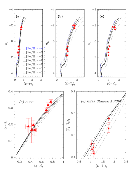
Figure 6: CMDs and colour-colour plots using a mixture of SDSS and Washington filters to show the [Fe/H]-sensitivity (HWD). In all diagrams, the red triangles are the 8 RGB stars, known to be proper-motion members. All isochrones shown are solar-scaled and have an age of 12 Gyr. (a) $M_{r}\;vs.\;(g-r)_{0}$ with Dartmouth models, $\alpha$-enhanced to +0.3. (b) $M_{T_{1}}\;vs.\;(C-T_{1})_{0}$ with Dartmouth models, also $\alpha$-enhanced to +0.3. (c) $M_{r}\;vs.\;(C-r)_{0}$ (d) $(r-i)_{0}\;vs.\;(g-r)_{0}$ SDSS colour-colour plot, with the Dartmouth isochrones. (e) Washington colours with GS99 standard giant branches (HWB).

6 Discussion

From Figure 6b, we see that $(C-T_{1})$ widens the separation of the giant branches of different metallicities, giving a resolution for the GS99 RGB fiducial lines of $\sim 0.15$ dex. One of us (GW) suggested the Washington system, which was developed by Canterna (1976); Geisler (1996) defined CCD standard fields for the system. In HWB, we found that Washington filters spread out the stars at the MSTO, and we have found that $(C-T_{1})$ is more effective than the SDSS-colours $(g-r)$, as shown in Figure 6a. The SDSS photometry is not sensitive enough to this difference in colours to distinguish Boo I’s level of metallicity spread. The subset of 19 objects with $ugriz$ magnitudes (Table 4) contains most of the bright objects from HWB and this paper’s Strömgren data set. These are the objects which have Strömgren and Washington colours falling in the appropriate ranges which enable us to calculate the photometric values of $[Fe/H]$. Table 3 contains foreground stars and Boötes I members, and intersects with the spectroscopic data set of Martin et al. (2007). We have radial velocities and independent metallicities for 8 of the objects in Table 3, and Strömgren and Washington $[Fe/H]_{phot}$-values for many of them. We added the 2 giants outside the central Boötes I field, Boo-1137 and Boo-127, as additional calibrators, because Boo-1137 (Norris et al., 2010b) is very metal poor, and both have had a number of spectra taken (see Table 5).

We considered the effect of replacing the $g$-filter with the much broader $C$-band (Hughes & Wallerstein, 2011a). As we can see from Figure 6b and 6c, the colour, $(C-r)$ works well for the upper RGB ($\log g<1.5$) in Boötes I, but that the lower-RGB stars ($2.5<\log g<3.0$) are not well-separated in this colour. The reasons for this discrepancy are filter-width and transmission, which are shown in Figure 2a and Table 2. While the Sloan $r$-filter has a greater overall transmission than the Washington $T_{1}$-filter, it has become standard practice to substitute the broadband $R$-filter for $T_{1}$, since it has $\Delta\lambda_{R}=1580$Å, compared to $\Delta\lambda_{T_{1}}=770$Å (Geisler, 1996, also see Table 2).

As with the Lai et al. (2011) method, there are merits in combining all the available photometry, but we are searching for the minimum useful number of filters that can break the age-metallicity degeneracy. In Figure 7, we compare the Strömgren and Washington filters, and construct two new indices:

$$m_{*}=(C-T_{1})_{0}-(T_{1}-T_{2})_{0}$$ (26)

and

$$m_{**}=(C-b)_{0}-(b-y)_{0}.$$ (27)

Our motivation in defining these indices is to avoid the collapse of the metallicity sensitivity of the $m_{1}$-index on the lower RGB, and to attempt to replace the $v$-filter with the broader $C$-filter (also see Hughes & Wallerstein, 2011a). Figure 7h shows $m_{**}\;vs.\;(C-T_{1})_{0}$, and allows us to use 4 filters, $CT_{1}by$, which reduces observing time and keeps $\sim 0.3$ dex [Fe/H]-resolution for stars with $-1.5>[Fe/H]>-4.0$. Figure 7i shows that we could use $Cby$ for metallicity estimates $-1.5>[Fe/H]>-4.0$. These colour-colour plots are not sensitive to age on the RGB, recovering age-resolution at the MSTO. However, reaching the MSTO with $Cby$ is much faster than with $vby$ (see Table 2). Figs.7a, b & c show that $m_{0}$ may be preferred for systems with $-1.0>[Fe/H]>-2.0$, but we note that $(C-T_{1})$ would also be more useful there, with much shorter exposure times.

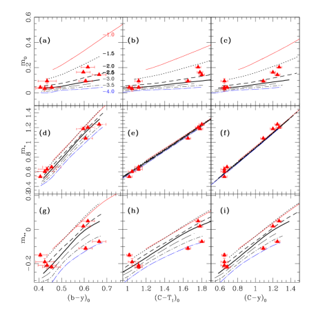
Figure 7: Colour-colour plots using a mixture of Strömgren and Washington filters to show the [Fe/H]-sensitivity. In all plots, the red triangles are the 8 RGB stars from proper-motion studies (Martin et al., 2007), and we show the Dartmouth models in the range, $-1.0>[Fe/H]>-4.0$. We define: $m_{*}=(C-T_{1})_{0}-(T_{1}-T_{2})_{0}$ and $m_{**}=(C-b)_{0}-(b-y)_{0}$, with dereddened-$m_{1}$ written as $m_{0}=(v-b)_{0}-(b-y)_{0}$. (a) $m_{0}\;vs.\;(b-y)_{0}$. (b) $m_{0}\;vs.\;(C-T_{1})_{0}$. (c) $m_{0}\;vs.\;(C-y)_{0}$. (d) $m_{*}\;vs.\;(b-y)_{0}$. (e) $m_{*}\;vs.\;(C-T_{1})_{0}$. (f) $m_{*}\;vs.\;(C-y)_{0}$. (g) $m_{**}\;vs.\;(b-y)_{0}$. (h) $m_{**}\;vs.\;(C-T_{1})_{0}$. (i) $m_{**}\;vs.\;(C-y)_{0}$.

6.1 SPECTRAL ENERGY DISTRIBUTIONS OF INDIVIDUAL STARS

When crossing the boundaries between photometric systems, we found it instructive to construct SEDs for our sample, as a independent and external check on our photometry and to make sure all the magnitudes were on their standard systems (Bessell, 2005). This process enabled us to compare the Dartmouth models and the ATLAS9 synthetic stars to the real data, and understand better the constraints placed by the observational uncertainties and the relationship between each stars’ temperature and metallicity. Figures 8–15 display SEDs for the 8 RGB proper-motion confirmed members of Boötes I  shown with the best-fitting (employing a simple $\chi^{2}$ fit) ATLAS9 model fluxes, appropriately scaled to pass through the majority of the photometry data points. If there is a wide discrepancy between the fits to the ATLAS9 models in Washington, Strömgren, and SDSS filters, we show 2 fits. The y-axes are always flux density, log($\nu F_{\nu}$), in ergs/s/cm, and the x-axes are wavelength in microns. We used the conversions from magnitudes to fluxes from the HST ACS website. The Washington system and the Strömgren data are VEGAmag and the SDSS system is ABmag, and we determined that the 8 RGB stars had the fluxes transformed to the same scale for Washington, Strömgren, and SDSS magnitudes, without any further shifting, except for HWB-22, where the SDSS fluxes are consistently higher. Since the Washington and Strömgren data appeared to be consistent with the same $T_{eff}$ for HWB-22, we did not shift any of our zero-point scales. As expected, our photometry uncertainties produce smaller error bars than the SDSS data, and these stars also suffer from large uncertainties in SDSS-u. Where available, we include the 2MASS, $JHK$ measurements.

In all diagrams, the SDSS data is shown as open squares, the Strömgren measurements are shown as small filled triangles, Washington magnitudes are the larger filled triangles, and 2MASS data (if available) is shown as open stars. The error bars are the $1\sigma$ uncertainties in the data. If there was a Johnson-V observation, it is shown as an open circle.

Boo-1137 (Figure 8) is the brightest object in this sample, and the most metal-poor, reported to be $[Fe/H]=-3.7$, by Norris et al. (2010b), who obtained high-resolution spectroscopy of from VLT/UVES. This star was not originally in our data set because it is 24^′ from the center of the dSph. Norris et al. (2010b) pronounced it the most metal-poor giant observed (to-date) in one of the ultra-faint SDSS dSphs, and show that Boo-1137’s elemental abundances are similar to those seen in metal-poor Milky Way halo stars. Given the range in fits from Table 5, we show the ATLAS9 model-range which fit the data best, i.e. very metal-poor, $T_{eff}=4750K$, $[Fe/H]=-3.7$, $[\alpha/Fe]=+0.4$, and $\log g=1.4$.

Figure 8: Spectral-energy distribution of Boo-1137 shown with the best-fitting ATLAS9 (interpolated) model fluxes, appropriately scaled. The SDSS data is shown as open squares, the Strömgren measurements are shown as filled triangles, Washington magnitudes are the larger filled triangles, and 2MASS data is the open stars. The error bars are the $1\sigma$ uncertainties in the data. (a) SED for the range in wavelength, $0.1\mu m<\lambda<2.3\mu m$. (b) SED for the range in wavelength, $0.3\mu m<\lambda<1.0\mu m$.

Figure 9: Spectral-energy distribution of Boo-127 shown with the best-fitting ATLAS9 (interpolated) model fluxes, appropriately scaled. The SDSS data is shown as open squares, the Strömgren measurements are shown as filled triangles, Washington magnitudes are the larger filled triangles, and 2MASS data is the open stars. The error bars are the $1\sigma$ uncertainties in the data. The Johnson-$V$ observation is is shown as an open circle. (a) SED for the range in wavelength, $0.1\mu m<\lambda<2.3\mu m$. (b) SED for the range in wavelength, $0.3\mu m<\lambda<1.0\mu m$.

Figure 10: Spectral-energy distribution of Boo-117/HWB-8 shown with the best-fitting ATLAS9 (interpolated) model fluxes, appropriately scaled. The SDSS data is shown as open squares, the Strömgren measurements are shown as filled triangles, Washington magnitudes are the larger filled triangles, and 2MASS data is the open stars. The error bars are the $1\sigma$ uncertainties in the data. The Johnson-$V$ observation is shown as an open circle. (a) SED for the range in wavelength, $0.1\mu m<\lambda<2.3\mu m$. (b) SED for the range in wavelength, $0.3\mu m<\lambda<1.0\mu m$.

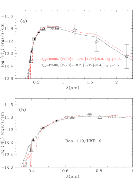
Figure 11: Spectral-energy distribution of Boo-119/HWB-9 shown with the best-fitting ATLAS9 (interpolated) model fluxes, appropriately scaled. The SDSS data is shown as open squares, the Strömgren measurements are shown as filled triangles, Washington magnitudes are the larger filled triangles, and 2MASS data is the open stars. The error bars are the $1\sigma$ uncertainties in the data. (a) SED for the range in wavelength, $0.1\mu m<\lambda<2.3\mu m$. (b) SED for the range in wavelength, $0.3\mu m<\lambda<1.0\mu m$.

Figure 12: Spectral-energy distribution of HWB-22 shown with the best-fitting ATLAS9 (interpolated) model fluxes, appropriately scaled. The SDSS data is shown as open squares, the Strömgren measurements are shown as filled triangles, Washington magnitudes are the larger filled triangles. The error bars are the $1\sigma$ uncertainties in the data. (a) SED for the range in wavelength, $0.1\mu m<\lambda<2.3\mu m$. (b) SED for the range in wavelength, $0.3\mu m<\lambda<1.0\mu m$.

Figure 13: Spectral-energy distribution of HWB-24 shown with the best-fitting ATLAS9 (interpolated) model fluxes, appropriately scaled. The SDSS data is shown as open squares, the Strömgren measurements are shown as filled triangles, Washington magnitudes are the larger filled triangles. The error bars are the $1\sigma$ uncertainties in the data. (a) SED for the range in wavelength, $0.1\mu m<\lambda<2.3\mu m$. (b) SED for the range in wavelength, $0.3\mu m<\lambda<1.0\mu m$.

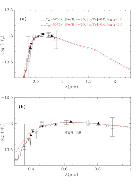
Figure 14: Spectral-energy distribution of HWB-28 shown with the best-fitting ATLAS9 (interpolated) model fluxes, appropriately scaled. The SDSS data is shown as open squares, the Strömgren measurements are shown as filled triangles, Washington magnitudes are the larger filled triangles. The error bars are the $1\sigma$ uncertainties in the data. (a) SED for the range in wavelength, $0.1\mu m<\lambda<2.3\mu m$. (b) SED for the range in wavelength, $0.3\mu m<\lambda<1.0\mu m$.

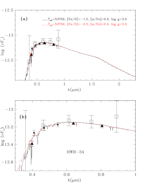
Figure 15: Spectral-energy distribution of HWB-34 shown with the best-fitting ATLAS9 (interpolated) model fluxes, appropriately scaled. The SDSS data is shown as open squares, the Strömgren measurements are shown as filled triangles, Washington magnitudes are the larger filled triangles. The error bars are the $1\sigma$ uncertainties in the data. (a) SED for the range in wavelength, $0.1\mu m<\lambda<2.3\mu m$. (b) SED for the range in wavelength, $0.3\mu m<\lambda<1.0\mu m$.

Boo-127 (Figure 9) was found to have an unusual [Mg/Ca] abundance ratio, similar to the Hercules dSph (Feltzing et al., 2009). Feltzing et al. (2009) found $[Fe/H]=-1.98$, while Norris et al. (2008) found $[Fe/H]=-1.49$. From the spectroscopy in Table 5 and isochrone fits in Table 9, we find that $[Fe/H]=-2.0$ across all the filter-systems and that the best ATLAS9 fits are models, with $T_{eff}=4750K$, $[Fe/H]=-2.0$, $[\alpha/Fe]=+0.4$, and $\log g=1.3$. However, Norris et al. (2010a) later obtained UVES/FLAMES data for Boo-127, where they reported, $[Fe/H]=-2.08$; with a mean error of about 0.27 dex. Gilmore et al. (2013b) concurs, so we can conclude that the spectroscopic $[Fe/H]$-values are now in agreement.

Boo-117/HWB-8 (Figure 10) has the most independent observations. Norris et al. (2008) measured $[Fe/H]=-1.72$, using the calibration from the strength of the Ca II K line, and found $[Ca/Fe]\sim 0.3$. This value was more metal-rich than the $[Fe/H]=-2.2$ noted by Martin et al. (2007), and is at least 0.4 dex more metal-rich than any of our other photometric estimates. Feltzing et al. (2009) reported a value of $[Fe/H]=-2.24$ for Boo-117 (HIRES; using the Fe lines, amongst others), that is more consistent with our Strömgren data. As discussed in Feltzing et al. (2009), even different spectroscopic surveys can vary from $0.3$ to $0.5$ dex, so we should not be surprised by this. We show the ATLAS9 models/interpolations, with $T_{eff}=4625K$, $[Fe/H]=-2.25$ & $[\alpha/Fe]=+0.2$ & $\log g=1.25$. We note that the bluer photometry points are more consistent with a slightly more metal-rich spectrum, but that all the fits are well-within the uncertainties stated in the spectroscopic studies. Also, Lai et al. (2011) derive $[Fe/H]=-2.3$ and $[C/Fe]=-0.5$, from their low resolution spectra, SDSS and other filters with the n-SSPP code.

Boo-119/HWB-9 (Figure 11) is a star we expected to have inconsistent photometric estimates, since Martin et al. (2007, Boo-119) derived $[Fe/H]=-2.7$, and the isochrone fits to each filter set range into the more metal-rich regime: $[Fe/H]=-2.0$ for the SDSS filters, The Washington filters give $[Fe/H]=-1.7$, and we find $[Fe/H]=-1.5$ from the Strömgren isochrones. We expected this discrepancy to be a characteristic of a CN- or carbon-rich star, and Lai et al. (2011) report $[Fe/H]=-3.8$ and $[C/Fe]=+2.20$. The best-fit ATLAS9 models indicate an interpolation in the range $T_{eff}=4625K-4750K$, $[Fe/H]=-1.8$ to $-2.5$, $[\alpha/Fe]=+0.2$ to $+0.4$, and $\log g=1.5$. The model with $T_{eff}=4750K$ and $[Fe/H]=-2.5$, has the smallest residuals, and is consistent with the CaT-measurement from Martin et al. (2007). We show the range of models with $T_{eff}=4600-4750K$, $[Fe/H]=-1.75$ to $-3.7$, $[\alpha/Fe]=+0.2$ to $+0.4$, and $\log g=1.5$.

HWB-22 (Figure 12) may be variable. There is no clear offset in the photometry points between the different filter systems for any of the other RGB stars, but it does seem be the case here. Martin et al. (2007) give $[Fe/H]=-2.2$, Lai et al. (2011) give $[Fe/H]=-2.9$ and $[C/Fe]<0.0$, and our isochrone fits give $[Fe/H]=-2.0$ to $-3.0$. The ATLAS9 models indicate the best fit is: $T_{eff}=5250K$, $[Fe/H]=-2.0$, $[\alpha/Fe]=+0.4$, and $\log g=2.5$. The difference in photometry could be caused by a temperature difference, but that the metallicity and surface gravity measurements are all consistent with each other. We chose to show the fit to the Strömgren and Washington colours.

HWB-24 (Figure 13) The GS99 calibration gives $-3.0\pm 1.0$ dex, and adds no further information. The GS99 standard RGB’s (and the Dotter et al. 2008 models in Washington filters) become insensitive to very low metallicities amongst the brighter RGB stars much more rapidly than the Strömgren calibrations. For Washington data on low-metallicity systems, it is better to use the CMDs than the colour-colour plots, since the models separate better in luminosity and $(C-T_{1})$ than they do in $(T_{1}-T_{2})$. At this level on the RGB, the Strömgren calibration starts to lose sensitivity.

HWB-28 (Figure 14) fits the SDSS isochrones and the Lai et al. (2011) models both with$[Fe/H]\geq-2.5$, but the Strömgren-fit gives $[Fe/H]=-1.7$. The fit from the Washington filters gives $[Fe/H]=-1.5$, closer to the Martin et al. (2007) estimate $[Fe/H]=-1.5$ from the CaT-method. From the ATLAS9 models, we can see the why the SDSS filters can indicate a much more metal-poor model than the Strömgren filters and the C-band. Note that the g-band error bars encompass both model SEDs, $T_{eff}=5250K-5375K$, $[Fe/H]=-1.5$ and $-2.5$, $[\alpha/Fe]=+0.2$ and $+0.4$, and $\log g=3.0$. This temperature range makes the dashed line fit the SDSS photometry with smaller residuals than the more metal-rich case.

HWB-34 (Figure 15) has a consistent ATLAS9 model temperature, with $T_{eff}=5375K$, and we show $[Fe/H]=-1.3$ and $-2.5$, $[\alpha/Fe]=+0.2$ and $+0.4$ , and $\log g=3.0$. Lai et al. (2011) fit $[Fe/H]=-2.4$, Martin et al. (2007) find $[Fe/H]=-1.3$. The Strömgren system isochrones yield $[Fe/H]=-2.0$ and the $CT_{1}T_{2}$-photometry gives $[Fe/H]=-1.7$. This star is at the exactly the right (or in this case, wrong) part of the temperature/metallicity distribution to make it very difficult to discern where this star falls within $[Fe/H]=-1.7\pm 0.5$ dex, and the deciding factor would be the $C$- or $v$-magnitude.

6.2 COMPARISON WITH SIMPLE MODELS

For the 8 Boötes I  radial-velocity-confirmed members (Table 5), the photometric metallicities that were most discrepant were for the fainter objects on the lower RGB, as we expected. However, Boo-119/HWB-9’s (Figure 11) discrepancies are likely due to carbon-enhancement. We now compare the spectroscopic metallicities to those found from different filter sets and hybrid methods. Table 5 shows a clear offset from the [Fe/H]-values from the spectroscopy-alone studies (Gilmore et al., 2013b; Norris et al., 2010b; Feltzing et al., 2009; Martin et al., 2007; Hughes, Wallerstein & Bossi, 2008), but that shift to lower $[Fe/H]$ was discussed in §2, and is partly to do with scaling changes over time and calibration of CaT-measurements. Apparently, no photometric system can cope with Boo-119’s carbon-iron abundance ratio, $[C/Fe]=+2.20$, except for Lai et al.’s (2011) modified n-SSPP method, which skews all [Fe/H]-estimates lower than any scale based on CaT alone (Koposov et al. (2011) notes that their scale is not calibrated below $[Fe/H]=-2.5$)

Feltzing et al. (2009) discuss their spectroscopy of Boötes I, in light of work by Koch et al. (2008) on the Hercules dSph. In these dark-matter dominated dSphs, the very low density of baryons should mean that the chemical enrichment history is dominated by only a “few supernovae”, which means that the element abundances of the stellar population might show star-to-star chemical inhomogeneities, tracing individual SNe II events (Gilmore et al., 2013a, b). In studying the Hercules system, Koch et al. (2008) estimate that only 10 SN were needed to give the “atypical abundance ratios” (and more should have contributed). Boötes I is less massive than Hercules, but Feltzing et al. (2009) only report one star, Boo-127, (and possibly Boo-094, also not observed here), has unusual variations in Mg and Ca. Expecting more individuality, Feltzing et al. (2009) conclude that Boötes I is surprisingly well-mixed. Norris et al. (2009) beg to differ, and they take issue with Feltzing et al.’s (2009) $[Mg/Ca]$ value as being too high for one of their seven Boötes I stars, the aforementioned, Boo-127. We agree with Norris’s group, and also Gilmore et al. (2013b).

Norris et al. (2009) obtained high-resolution spectroscopy of Boo-1137 from VLT/UVES (not included in HWB’s data set because it is $24^{\prime}$ from the center of the dSph), pronouncing it the most metal-poor giant observed (to-date) in one of the ultra-faint SDSS dSphs, with $[Fe/H]=-3.7$. Norris et al. (2009) find that Boo-1137’s elemental abundances are similar to those seen in metal-poor MWG halo stars. They also discuss Boötes I’s SF history, surmising that it most likely underwent an early, short period of star formation, cleared by SN II which enriched it’s interstellar medium inhomogeneously. In Boo-1137, Norris et al. (2009) find $\alpha$-enhancement (compared to Fe) of $\Delta[\alpha/Fe]\sim 0.2$, “relative to the mean of the metal-poor halo stars.” Even though the spectroscopy studies we have mentioned have tried to cover as much of the Boötes I  dSph as possible (and Boo-1137 is almost two half-light radii from the center), all groups have collected medium resolution spectra of less than 30 members, with high-resolution spectra of only a handful of stars. As Tolstoy, Hill & Tosi (2009) and Gilmore et al. (2013a) say, SNe Ia start to contribute to the chemical composition $10^{8}-10^{9}$ years after the first stars form. There is a wide range in $[Fe/H]$, but not in the $\alpha$-elements. So, if the massive stars in Boötes I cleared the interstellar medium quickly, star formation lasted less than 1 Gyr. Can we detect an age spread that small?

Table 5: Metallicities of Possible Boötes I Stars

ID	$[Fe/H]_{Hil}^{1}$	$[Fe/H]_{m_{1}}^{2}$	$[Fe/H]_{[m]}^{3}$	$[Fe/H]_{GS}^{4}$	$[Fe/H]_{spec}^{5}$				$[\alpha/Fe]_{Gil}^{6}$	$[Fe/H]_{Lai}^{7}$	$[C/Fe]_{Lai}^{7}$
Boo-1137	$-2.1(0.3)$	-2.4	-2.3	$-2.2(0.3)$	-3.7	$-$	-3.66	y	0.44	$-$	$-$
Boo-127	$-2.0(0.3)$	-2.2	-2.2	$-2.0(0.3)$	-1.49	$-$	-2.01	y	0.18	$-$	$-$
Boo-117/HWB-88	$-1.6(0.3)$	-1.9	-1.8	$-2.0(0.3)$	-1.72	-2.2	-2.18	y	0.18	-2.3	-0.50
Boo-119/HWB-9	$-1.5(0.3)$	-1.7	-1.7	$-2.0(0.3)$	$-$	-2.7	-3.33	y	0.77	-3.8	+2.20
HWB-16	$-1.8(0.6)$	-2.2	-2.2	$-2.6(0.5)$	$-$	$-$	$-$	u	$-$	$-$	$-$
HWB-19	$-0.5(1.0)$	-0.5	-0.6	$-3.3(0.8)$	$-$	$-$	$-$	n	$-$	$-$	$-$
HWB-22	$-1.8(0.6)$	-2.3	-2.3	$-2.9(0.7)$	$-$	-2.0	$-$	y	$-$	-2.9	$<0.00$
HWB-24	$-1.4(0.7)$	-2.0	-2.0	$-3.0(0.7)$	$-$	-1.9	$-$	y	$-$	-2.3	+0.40
HWB-28	$-1.2(0.6)$	-1.6	-1.6	$-2.9(0.6)$	$-$	-1.5	$-$	y	$-$	-2.5	+0.39
HWB-29	$-1.4(0.9)$	-1.8	-1.7	$-2.8(0.6)$	$-$	$-$	$-$	u	$-$	$-$	$-$
HWB-31	$-2.3(0.9)$	-3.8	-3.6	$-3.1(0.8)$	$-$	$-$	$-$	u	$-$	$-$	$-$
HWB-34	$-1.7(0.9)$	-2.3	-2.3	$-3.0(0.7)$	$-$	-1.3	$-$	y	$-$	-2.4	+0.34
HWB-40	$-1.6(0.9)$	-2.1	-2.1	$-2.9(0.7)$	$-$	$-$	$-$	u	$-$	$-$	$-$

(1) From photometry: Strömgren-$[Fe/H]$ calibration from Hilker (2000).

(2) From photometry: Strömgren-$[Fe/H]$:– $m_{1}$ calibrations from Calamida et al. (2007), uncertainties are $\sim 60\%$ greater than the Hilker (2000) calibration.

(3) From photometry: Strömgren-$[Fe/H]$:– [m] calibrations from Calamida et al. (2007).

(4) From photometry: averaging GS99’s standard RGB-calibrations, since there is a spread in metallicity.

(5) From spectroscopy, respectively: Norris et al. (2008); Martin et al. (2007); Gilmore et al. (2013b). Proper motion membership designated: yes=y; no=n; unknown=u.

(6) Gilmore et al. (2013b)

(7) From photometry and spectroscopy Lai et al. (2011) n-SSPP method.

(8) Boo-117 appears in Martin et al. (2007); Norris et al. (2008); Feltzing et al. (2009). Gilmore et al. (2013b) prefers $[Fe/H]\sim-2.2.$

Table 6: Fitted Parameters for Boötes I Stars from Hughes & Wallerstein (2011b)

ID	$[Fe/H]_{Spec}^{1}$	$[Fe/H]_{phot}^{2}$	$T_{eff}(K)^{3}$	$\log g^{4}$	Age (Gyr)5
Boo-117/HWB-8	-2.25	-2.4	4700	1.4	11
Boo-119/HWB-9	-2.7	-2.7	4750	1.5	12
HWB-22	-2.2	-2.2	5250	2.6	12
HWB-24	-1.9	-1.8	5300	2.7	12
HWB-28	-1.5	-1.2	5350	2.9	11
HWB-34	-1.3	-1.1	5400	3.1	12

(1) From Martin et al. (2007).

(2) Means found from fitting Washington and Strömgren photometry separately to the $\alpha$-enhanced Dartmouth isochrones, then taking weighted means, dependent on error bars. Uncertainties are then $\pm 0.25$ dex.

(3) Weighted mean from Dartmouth isochrones, uncertainties are $\pm 50K$.

(4) Weighted mean from Dartmouth isochrones, uncertainties are $\pm 0.05$ dex.

(5) Weighted mean from Dartmouth isochrones, uncertainties are $\pm 1.0$ Gyr.

Table 7: Model Fits for $-1.8>[Fe/H]>-2.5$ and Constant Age of 11.5 Gyr, $[\alpha/Fe]=0.0$

$\Delta$colour/Index	MSTO	RGB	rRGB
(mag.)	$M_{T_{1}}\sim 3$	$M_{T_{1}}\leq-1.5$	$2>M_{T_{1}}>1$
$(C-T_{1})$	0.267	0.557	0.247
$(T_{1}-T_{2})$	0.080	0.106	0.047
$(b-y)$	0.073	0.157	0.057
$m_{1}$	0.024	0.115	0.045
$[m]$	0.014	0.162	0.054
$m_{*}$	0.187	0.451	0.199
$m_{**}$	0.051	0.133	0.092
$(C-y)$	0.196	0.447	0.202
$(u-g)$	0.039	0.519	0.192
$(g-r)$	0.139	0.221	0.099
$(r-i)$	0.071	0.091	0.064
$(B-V)^{\dagger}$	0.203	0.341	0.193
$(V-R)^{\dagger}$	0.122	0.201	0.116
$(V-I)^{\dagger}$	0.252	0.401	0.242

Non-$\alpha$-enhanced models generated from the Dartmouth isochrones (Dotter et al., 2008). ^†From Table 4 of Geisler (1996), converting $(C-T_{1})$ to BVRI colours.

What kind of metallicity or age spread would we expect to see in Boötes I? Age estimates cannot usually be made for individual RGB stars, but the GS99 standard giant branches do have an age-metallicity degeneracy, compared to the Dartmouth isochrones. Is the separation of RGB stars with Boötes I’s range in chemical composition, large enough to differentiate between RGB-isochrones in any colour? Our normal practice is to use the RGB to find the metallicity and the MSTO to find ages, where the isochrones separate. Brown et al. (2012) and Kirby et al. (2012) studied the metallicity distributions and star formation histories (SFHs) of several dSphs. Isochrone fits to these populations, as noted by Kirby, have to be performed at the upper-RGB, the SGB and the MSTO, in order to break the age-metallicity degeneracy. In many dSphs, we do not have sufficient upper-RGB stars to make this fit (Willman, 2010).

Table 8: colour Change/Gyr for Model Fits for Constant $[Fe/H]=-1.8$, $[\alpha/Fe]=0.0$, and Age Range of 10-14 Gyr

$\Delta$colour/Index	MSTO	RGB	rRGB
(mag.)	$M_{T_{1}}\sim 3$	$M_{T_{1}}\leq-1.5$	$2>M_{T_{1}}>1$
$(C-T_{1})$	0.129	0.417	0.016
$(T_{1}-T_{2})$	0.040	0.084	0.004
$(b-y)$	0.037	0.109	0.004
$m_{1}$	0.010	0.135	0.000
$[m]$	0.004	0.168	0.001
$m_{*}$	0.090	0.333	0.012
$m_{**}$	0.027	0.111	0.003
$(C-y)$	0.095	0.329	0.012
$(u-g)$	0.008	0.413	0.014
$(g-r)$	0.072	0.170	0.007
$(r-i)$	0.008	0.076	0.003
$(B-V)^{\dagger}$	0.137	0.274	0.084
$(V-R)^{\dagger}$	0.084	0.163	0.053
$(V-I)^{\dagger}$	0.181	0.329	0.123

Non-$\alpha$-enhanced models generated from the Dartmouth isochrones (Dotter et al., 2008). ^†From Table 4 of Geisler (1996), converting $(C-T_{1})$ to BVRI colours.

To improve the resolution of our grid of Dartmouth isochrones, we ran a simple closed-box chemical evolution mode. We used the Dartmouth (solar-scaled) isochrones to produce populations of stars with a similar physical size, mass, and metallicity spread to Boötes I, but with ages of 10–14 Gyr over the approximate metallicity range $-1.0>{Fe/H}>-4.0$. We obtained over 50,000 artificial stars (binary fraction of 0.5) with Strömgren, Washington and SDSS magnitudes. We compared model stars with our objects having $vbyCT_{1}T_{2}$ measurements.

From these model runs, we chose 3 simple cases. Firstly, there is a single-age (11.5 Gyr) population (1216 stars), with a conservative spread in metallicity from $[Fe/H]=-3.5$ up to $-1.5$. We call this Case I. The second population (Case II: 9133) was designed to be enriched in situ, with $-4.0<[Fe/H]<-1.0$. The metallicity distribution terminated after star formation lasting at least 4 Gyr. We added Case III, an alternative long-duration population with a few “starbursts,” to determine if we could tell it apart from Case II. In Case III, there are 1374 stars born 12 Gyr ago, with $-3.5<[Fe/H]<-2.5$, 6375 stars with $-2.5<[Fe/H]<-1.75$, which are 0.5 Gyr younger, and 1363 stars with $-1.75<[Fe/H]<-1.0$, with SF extending up to 10 Gyr ago, and then terminating. Using the Kolmogorov-Smirnov Test for Two Populations, where the null-hypothesis ($H_{0}$) is that the populations are the same, we can tell the difference between the age spreads in Cases I, II and III, but not the metallicity ranges.

In order to make the models more realistic, we use the photometric uncertainties from Figure 3. From tests, we found that we required at least 2% photometry at the MSTO to determine if there are age spreads present, since the isochrones exhibit a change of $\sim 0.06$ mag. in $(C-T_{1})$ for each Gyr in age. There would have to be much deeper Strömgren photometry for any age spread less than 1.5 Gyr to be distinguished. In the Washington system alone, with $[Fe/H]\sim-2.0$, 2 per cent photometric uncertainty at the MSTO would reveal an age spread of $>1$ Gyr.

We selected models with $\log g$ of 1.0-2.0 for the RGB stars, 2.0-3.0 for the rising-RGB (rRGB), below the level of the HB, and $\log g\sim 4.0$ for the MSTO. We examined the colours in the Strömgren, Washington and SDSS systems, at fixed age and fixed-[Fe/H]. Our goal was to quantify the filter systems sensitivity and break the age-metallicity degeneracy as cleanly as possible, avoiding the upper-RGB. The results of the artificial star experiments are given in Tables 7 and 8, and Figure 16. Figure 16a shows colours and indices for the stars in all the models with an age of 11.5 Gyr, and examines a range of $-2.5<[Fe/H]<-1.8$. The RGB stars’ range is shown in orange, the rRGB in gold, and the MSTO in violet. Figure 7b takes stars at a constant $[Fe/H]=-1.8$. We know that the real stars are $\alpha$-enhanced at the +0.2 to +0.4 dex level, Norris et al. 2010b and Gilmore et al. 2013b; see Table 5 which would make a metal-poor star look more metal rich in the broad-band colors. In Figure 16b, we let the model stars have a fixed metallicity value of $[Fe/H]=-1.8$ (more like a real sample of $[Fe/H]\geq-2.0$) and let the age vary from 10-14 Gyr.

Even though these models cannot be considered well-calibrated below $[Fe/H]=-2.5$, we show the lower end of the $[Fe/H]$-range, from $-4.0<[Fe/H]<-3.0$, at a constant age of 11.5 Gyr, but we hatch the bar-chart to recognize this factor. If we were fortunate to collect so many $[Fe/H]$-values of enough real stars in dSphs at this low range in $[Fe/H]$, the stars may be $\alpha$-enhanced and may not appear so metal-poor broadband colors (CN- or C-enhanced). However, this is the parameter-space where the SDSS-colors recover their usefulness. For our sample, that the SDSS-colors are very uncertain here, as the $u-$ and $g-$magnitudes have large uncertainties (see Table 4) returned are too low for the MSTO-stars, at the sensitive TO-value of $\log g$. If we had detections down to the MSTO stars, they would have a spread in $(u-g)\geq 3.0$. Here, the SDSS filters lack of sensitivity to $\alpha$-elements lets us recover a star’s metal-poor nature, even if it was an extreme example, e.g. Boo-119. However, for this color to be effective, the stars have to be detected at $SDSS-u$, which takes more than twice as long as the $C$-band (see Table 2). For stars just above the MSTO to the upper-RGB, $(C-T_{1})$ is most effective for all evolutionary stages in both age and metallicity. The $(C-T_{1})$ calibration loses is sensitivity below $[Fe/H]\sim-2.2$ on this scale, which is why we have to supplement it with $(b-y)$. The filter combination $CT_{1}by$, or even $Cby$, maintains its sensitivity to metallicity below $[Fe/H]\sim-3.0$, as can be seen in Figures 7g–i. Also note that the rRGB colours are hardly sensitive to age at all, and can be used to break the age-metallicity degeneracy. We want to avoid using Sloan-u or Strömgren-u, and the $v$-band, as both consume observing time (see Table 2). However, many searches for closer and brighter extremely metal-poor stars (Spite et al., 2013), this color could be vital, but even they use $(g-z)$ to avoid SDSS-u.

From the models, we find that the $(C-T_{1})$-colour is best for our sample above the MSTO; the $(C-y)$-colour is shown to be useful (in agreement with Ross et al. 2014), $m_{*}$ is better than $m_{**}$, and all these are better than the SDSS colours. However, constructing indices involves 3 or 4 filters, which increases the uncertainty in an parameters derived from a colour-colour or color-index calibration. The method of deriving age and $[Fe/H]$ will the smallest uncertainty is to use a color sensitive to temperature and one sensitive to chemical composition, but we need to combine the Washington and Strömgren filters.

We considered that Boötes I  might resemble $\omega$ Cen, the core of a captured dE, with extended enrichment and a long period of star formation (Gratton et al., 2011; Hughes et al., 2004). Due to its lack of HI or recent star formation (SF) (Bailin & Ford, 2007), we might expect Boötes I to have a simple history, similar to most globular clusters (Milone et al., 2012), with a short burst of star formation, terminated by supernovae (SNe) II events, or tidal stripping (Fellhauer et al., 2008) removing the ISM. This scenario should give rise to almost a single-age fit to the CMD, and a very narrow ($\Delta[Fe/H]<0.5$) dex metallicity range. Marcolini & D’Ercole (2008) discussed the model of Marcolini et al. (2006) which describes the chemical evolution of dSphs (particularly Draco, but it can be generalized). Marcolini & D’Ercole (2008) argue that the SNe II ejecta from the star formation event in a Draco-like dSph (actually about “50 instantaneous bursts” over 60 Myr) should be retained, due to the extra mass from the dark matter halo, and because “efficient radiative losses” keep the enriched ISM flowing back to the central regions of the dSph, mixing the gas. Cohen & Huang (2009) obtained high-resolution spectra of 8 stars in Draco, adding to 14 they had observed previously, which had a metallicity range of $-1.5>[Fe/H]>-3.0$ dex, similar to Boötes I; their age-metallicity relationship indicated that SF in Draco lasted about 5 Gyrs. An age spread even half this large should have been obvious for Boötes I, even with the uncertainties in Figure 3. The modeling of Draco’s enrichment history (Marcolini & D’Ercole, 2008), showed a star formation process lasting about 2 Gyr, with most of the initial Fe-enrichment coming from SNe II, with chemical inhomogeneities appearing later, caused by SNe Ia “pockets” of material, with higher $[Fe/H]$ and lower $[\alpha/Fe]$, which take 2–3 Gyr to mix in with the rest of the gas, the dynamics of which is driven by the SNe II effects. The discussion of possible star formation histories for this system is also illustrated by Gilmore et al. (2013a).

At the very least, the real Boötes I stars have $[\alpha/Fe]=+0.3\pm 0.1$ dex, but this value seems to be unchanging; it is likely that SF terminated before the onset of SN Ia contamination. We assume this can be quantified as a colour-shift. When we examined the Dartmouth isochrones, for $[\alpha/Fe]=0.0$ and $+0.4$, in the Strömgren system only the y-filter seemed to be sensitive to $[\alpha/Fe]$, making stars brighter by 0.046 mag. at 12 Gyr and $[Fe/H]=-2.5$. We saw that the model stars with low metallicities lost sensitivity in the $v$- and $b$-filters, making those magnitudes insensitive to $\alpha$-abundances. In the Washington filters, $T_{1}$ was shifted by -0.057 mag. and $(C-T_{1})$ by +0.035, with a variation of less than 1 per cent .

Table 9: Final Model Fits to Boötes I Stars

ID	Age(Gyr)	$[Fe/H]$	$T_{eff}(K)$	$\log g$
	$\pm 0.5$ Gyr	$\pm 0.3$ dex	$\pm 50$ K	$\pm 0.10$ dex
Boo-1137	12.0	-2.6	4775	1.34
Boo-127	10.8	-2.2	4743	1.38
Boo-117/HWB-8	10.6	-2.0	4684	1.42
Boo-119/HWB-9	10.8	-1.8	4705	1.49
HWB-16	11.5	-1.6	5022	2.21
HWB-19	11.5	-3.4	5292	2.91
HWB-22	11.5	-1.9	5184	2.60
HWB-24	11.5	-2.4	5314	2.77
HWB-28	11.5	-1.6	5288	2.89
HWB-29	11.5	-1.6	5298	2.92
HWB-31	12.0	-2.5	5422	3.03
HWB-34	11.5	-1.7	5365	3.10
HWB-40	11.6	-1.6	5411	3.49
HWB-45	12.0	-3.0	6919	4.07
HWB-47	11.9	-1.7	5574	3.51
HWB-48	11.5	-3.5	7022	4.17
HWB-50	11.5	-1.8	5709	3.62
HWB-51	11.5	-3.5	6948	3.91

$\chi^{2}$ fits to artificial stars generated from the $[\alpha/Fe]=0.0$ Dartmouth isochrones (Dotter et al., 2008), using the $CT_{1}by$-filters. Light cyan rows are confirmed members and the light gray row is a star that was ruled out by Martin et al. (2007) using its radial velocity.

Setting $[\alpha/Fe]\sim+0.4$ for Boötes I, we compare our Class A–C stars’ $CT_{1}by$-magnitudes with the whole data set of over 50,000 artificial stars, and the results are listed in Table 9. We performed $\chi^{2}$ fits to the stars generated from the $[\alpha/Fe]=0.0$ Dartmouth isochrones (Dotter et al., 2008), using the colour-shifts determined for the $CT_{1}by$-filters. With the possible inclusion of two blue stragglers (HWB-45 and HWB-51), and HWB-9 being carbon-rich (and CN-strong), the average age is $11.5\pm 0.4$ Gyr, and the range in metallicity is $-1.6>[Fe/H]>-3.4$, which would be shifted to around $-1.9>[Fe/H]>-3.7$ with $\alpha$-enhancement added back (in agreement with Gilmore et al., 2013b). We note that Boo-1137 does not appear as metal poor as it should, also, likely because the C-filter also loses sensitivity for very metal-poor stars. Our tests of the recovery of the artificial stars where we added typical photometric uncertainties found that the $(C-T_{1})$-colour started to become insensitive when $[Fe/H]<-2.2$. We also found it necessary to use $(b-y)$ as the temperature-sensitive colour instead of $(T_{1}-T_{2})$: otherwise, the temperatures of the real stars became at least 500K too hot compared to the SEDs shown in Figures 8–15. Using $m_{**}$ and $(b-y)$ or $(C-y)$ did not improve the fit. $(C-y)$ or $(C-T_{1})$ alone are not sufficient for individual stars, unlike whole giant branches (Ross et al., 2014).

We conclude that the fewest number of filters we can use for these old, metal-poor populations, is 4, and those are $CT_{1}by$. We preserve the $\sim 2$ dex range in [Fe/H] from the spectra, but we estimate Table 9’s $[Fe/H]$-values are, on average, 0.5 dex more metal-rich than Lai et al. (2011). Our results are more consistent with the CaT-calibrations, and the other spectroscopic studies (see Gilmore et al., 2012).

To display the observational uncertainties in derived parameters for Table 9, Figure 17 shows the CMDs in Strömgren, Washington, and SDSS filters for the model stars to match the real data shown in Figures 4 & 18. Starting with the black circles for Case II, with $-4.0<[Fe/H]<-1.0$ and ages, 10–14 Gyr. We then restrict the age range to 11-12 Gyr (green circles), and then to 11.3-11.7 Gyr (yellow). The green and yellow points have the same metallicity spread. Figure 17a–c are the models with no photometric scatter, and Figures 17d–f introduce the photometric uncertainty according to Figure 3 to match the Boötes I data (and if we had obtained similar SDSS-data instead of just the catalog magnitudes). We are able to detect the slight metallicity range contraction from the black points, $-4.0<[Fe/H]<-1.0$, to the green points $-3.0<[Fe/H]<-1.5$ at the SGB in Figure 17e, but not in the Strömgren filters in Figure 17d, as expected from Figure 16 and Tables 7 & 8. The vertical section of the MSTO is likewise able to detect the age contraction from a spread of 1 Gyr to 0.4 Gyr. We confirm that the SGB is sensitive to metallicity and not age, and the MSTO is more sensitive to age, except if we had very metal-poor with better than 1%-photometry in $(u-g)$ at the MSTO. We note that as the age spread contracts from the green to the yellow points for a few thousand stars in our models, and the RGB depopulates. The model-fits in Table 9 have a smaller value of $\chi^{2}$ when we use $(b-y)$ in addition to $(C-T_{1})$, rather than $T_{1}-T_{2}$. We conclude that only combining $CT_{1}by$ can cover this range in $[Fe/H]$ and age smoothly, with no break between the RGB and the MSTO stars, unless it is caused by photometric uncertainties. The uncertainties in Table 9 metallicities are $\pm 0.2~{}dex$ in $[Fe/H]$ and $\pm 0.3$ Gyr in age using 4 filters and with 1% photometry.

Figure 18 shows the final CMD with the $[\alpha/Fe]\sim+0.4$ Dartmouth isochrones. The Class A–C objects in Boötes I  have an age slightly less than 12 Gyr, but a wide [Fe/H]-range, likely exceeding 2 dex (Norris et al., 2008). It is possible to use the $(C-T_{1})$-colours alone, if the upper-RGB is well-populated and $[Fe/H]>-2.0$, to get age and metallicity (Ross et al., 2014). For most dSphs, with few stars on the upper-RGB, the rRGB and MSTO stars are sufficient to break the age-metallicity degeneracy, if you have 2 colours, $(C-T_{1})$) & $(b-y)$. Figure 17a shows that Strömgren colours are not sufficient alone to extract age information from the RGB with normal $\sim 1$ per cent photometry, and that high S/N is necessary at the MSTO to recover age information. We also note that Figure 18b shows $(C-T_{1})$ isochrones for $-1.0>[Fe/H]>-2.5$ maintain good separation for ages 10–12 Gyr, only having a pinch-point at the base of the RGB.

7 Conclusions

We have shown that the most efficient way to evaluate the metallicity, $[\alpha/Fe]$, and age of old, metal-poor systems is to observe individual stars with the $CT_{1}by$ filters combined with the Dartmouth isochrones. Application to the real Boötes I stars from Table 9 is as follows. If the distance and reddening are known, use the $T_{1}$-magnitude and the $(C-T_{1})$-colour to obtain $[Fe/H]$, $[\alpha/Fe]$, age, $\log T_{eff}$ and $\log g$ from a $\chi^{2}$-fit to the Dartmouth $\alpha$-enhanced course model-grid, with ages of (10, 12, & 14 Gyr). Primarily, this fixes $[\alpha/Fe]$ to $\pm 0.2$ dex for the star (or to see if $\alpha$-enhancement appears constant for the system). Then we use another $\chi^{2}$-fit model stars’ $T_{1}$-magnitudes, $(C-T_{1})$ and $(b-y)$ colours, to find the best-fit $[Fe/H]$, age, $\log T_{eff}$ and $\log g$ for each star. A recovery-test of this method returns over 90 per cent of the model stars if we add in 1–5% photometric errors. Noting that spectroscopic surveys do not always agree with each other (Gilmore et al., 2013a), our final estimates of $[Fe/H]$ from photometry agree with the spectroscopy measurements within $\sim 0.2$ dex. If the model stars have $[Fe/H]=-1.0$ to $-2.0$, then $T_{1}$-magnitudes and $(C-T_{1})$-colours are sufficient, and the metallicity of the whole system can be defined by the $m_{*}$-index. If $[Fe/H]<-2.0$, the $(b-y)$-colours need to be added and the metallicity alone can be found from $m_{**}$.

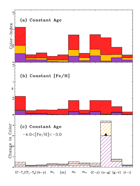
Figure 16: Proportional bar chart for the colour ranges for the models of RGB stars (red), with $\log g$ of 1.0-2.0; $\log g$ of 2.0-3.0 for the rising-RGB (rRGB; gold), below the level of the HB, and $\log g\sim 4.0$ for the MSTO (violet). The colours are shown for the Strömgren, Washington and SDSS systems, at: (a) fixed age of 11.5 Gyr and $-2.5<[Fe/H]<-1.8$. Data from Table 7. (b) Constant $[Fe/H]=-1.8$ (which would be equivalent to $\alpha$-enhanced more metal poor stars) and ages 10-14 Gyr. $(C-T_{1})$ is most effective for all evolutionary stages in both age and metallicity, and rRGB colours are insensitive to age. Data from Table 8. (c) Colour-range for models with a fixed age of 11.5 Gyr and $-4.0<[Fe/H]<-3.0$. Note that $(u-g)\geq 3.0$ becomes extremely sensitive for extremely metal-poor MSTO stars.

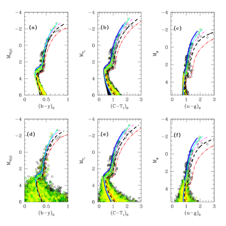
Figure 17: We show colour-magnitude diagrams for the Strömgren, Washington and SDSS data models. The Dartmouth isochrones for several values of $[Fe/H]$ and ages 10-12 Gyr are displayed. From left to right, the blue isochrones are $[Fe/H]=-4.0$, -3.5, and -3.0, $[\alpha/Fe]=+0.0$, all with an age of 12 Gyr, decreasing in thickness. The cyan line is $[Fe/H]=-2.5$, $[\alpha/Fe]=+0.4$ at 12 Gyr, the magenta dashed line is $[Fe/H]=-2.0$, $[\alpha/Fe]=+0.2$ at 12 Gyr, the black long-dashed line is $[Fe/H]=-1.5$, $[\alpha/Fe]=+0.0$, at 11 Gyr, and the red dot-dashed line is $[Fe/H]=-1.0$, $[\alpha/Fe]=+0.0$ at 10 Gyr. Here, the black circles are the 9133 stars from Case II with with $-4.0<[Fe/H]<-1.0$. The metallicity distribution terminated after star formation lasting at least 4 Gyr. Green circles are 3187 stars with ages 11-12Gyr and $-3.0<[Fe/H]<-1.5$. The yellow circles further restrict the age to 11.3-11.7 Gyr which shows the limits of age resolution for 1251 models stars. isochrones for several values of $[Fe/H]$ are displayed (a) Strömgren data for model stars with no added photometric scatter, but showing the broadened MS from the 0.5 binary fraction. (b) Washington CMD for the same sample. (c) Strömgren data with photometric scatter introduced according to Figure 3. (d) Washington CMD for the same sample, with the photometric scatter according to Figure 3.

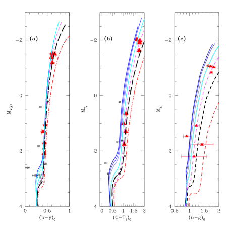
Figure 18: We show colour-magnitude diagrams for the Strömgren, Washington and SDSS data on Boötes I objects. The Dartmouth isochrones for several values of $[Fe/H]$ and ages 10-12 Gyr are displayed. From left to right, the blue isochrones are $[Fe/H]=-4.0$, -3.5, and -3.0, $[\alpha/Fe]=+0.0$, all with an age of 12 Gyr, decreasing in thickness. The cyan line is $[Fe/H]=-2.5$, $[\alpha/Fe]=+0.4$ at 12 Gyr, the magenta dashed line is $[Fe/H]=-2.0$, $[\alpha/Fe]=+0.2$ at 12 Gyr, the black long-dashed line is $[Fe/H]=-1.5$, $[\alpha/Fe]=+0.0$, at 11 Gyr, and the red dot-dashed line is $[Fe/H]=-1.0$, $[\alpha/Fe]=+0.0$ at 10 Gyr. In all plots, open circles are sources from Table 3 and the large red filled triangles represent the 8 proper motion-confirmed members. We use $E(B-V)=0.02$ and $DM=19.11$ for Boötes I. (a) The Strömgren CMD with stars from Table 3. (b) The Washington CMD with stars from Table 3. (c) The SDSS CMD shown with 8 proper-motion members from Table 4.

Our Boötes I data in Figure 18 is thus consistent with the models given the photometric scatter and that we can resolve the $[Fe/H]$-spread from at least -3.5 to -1.6, matching the ranges claimed by all the spectroscopic surveys. The large range in $[Fe/H]$, coupled with a small age range, which can be seen from combining the Strömgren and Washington data, indicates a short SF history. The best-fit isochrones and Figure 18 give an age for Boötes I of $11.5\pm 0.4$ Gyr, confirming that the ISM was lost at very early times. The spectroscopic surveys are not spatially uniform, but we agree with Gilmore et al. (2013a, b) and Koposov et al. (2011) that Boötes I seems to be comprised of more than one population distribution. A change in the $\alpha$-element abundances is not seen in their data or our isochrone fits, so that star formation is predicted to last at least 0.5 Gyr before any SN Ia contribute. The CEMP-no object (Boo-119) was likely to have formed from the ejecta of Pop III stars (Gilmore et al., 2013a, b), maybe only one also see Kirby et al., 2012.

We recommend that Washington filters are used for the study of dSph systems beyond $\sim 50$ kpc (Boötes I is at about 65 kpc), except where considerable reddening present; although they would still be better than $ugriz$. For future surveys using the Sloan filters, we recommend adding the Washington C-filter, as using $(C-r)$ is the best (and cheapest) compromise for comprehensive stellar population studies, but that $(u-g)$ is very effective at the MSTO. If a star is not carbon-enhanced, the $[Fe/H]$-sensitivity of the Washington and Strömgren combination ($CT_{1}by$) is at least twice as great as that of the SDSS filters. Below the horizontal branch, Strömgren and Washington filter sets lose metallicity sensitivity, but $CT_{1}by$ succeeds where other calibrations fail. For upper-red-giant branch stars, the Strömgren $m_{1}$-index gives a more-accurate metallicity estimate than the Washington filters compared to recent spectroscopic studies (around $\sim 0.3$ dex). Washington filters give better $[Fe/H]$-resolution for the range $-1.0>[Fe/H]>-2.0$, but for lower values, $[Fe/H]<-2.5$, $CT_{1}by$ is the most effective combination for these populations.

References

- Adelman-McCarthy et al. (2008) Adelman-McCarthy J. K. et al., 2008, ApJS, 175, 297
- Árnadóttir, Feltzing & Lundström (2010) Árnadóttir A. S., Feltzing S., Lundström I., 2010, A&A, 521, A40
- Bailin & Ford (2007) Bailin J., Ford A., 2007, MNRAS, 375, L41
- Belokurov (2013) Belokurov V., 2013, New Astrononomy Reviews, 57, 100
- Belokurov et al. (2006a) Belokurov V. et al., 2006a, ApJL, 642, L137
- Belokurov et al. (2006b) Belokurov V. et al., 2006b, ApJL, 647, L111
- Benson et al. (2002) Benson A. J., Frenk C. S., Lacey C. G., Baugh C. M., Cole S., 2002, MNRAS, 333, 177
- Bessell (2005) Bessell M. S., 2005, AAR&A, 43, 293
- Bohlin (2012) Bohlin R. C., 2012, Flux Calibration of the ACS CCD Cameras IV. Absolute Fluxes. Tech. rep.
- Brown et al. (2012) Brown T. M. et al., 2012, ApJL, 753, L21
- Bullock, Kravtsov & Weinberg (2000) Bullock J. S., Kravtsov A. V., Weinberg D. H., 2000, ApJ, 539, 517
- Calamida et al. (2007) Calamida A. et al., 2007, ApJ, 670, 400
- Calamida et al. (2009) Calamida A. et al., 2009, ApJ, 706, 1277
- Calamida et al. (2012) Calamida A., Monelli M., Milone A. P., Bono G., Pietrinferni A., Lagioia E. P., 2012, A&A, 544, A152
- Canterna (1976) Canterna R., 1976, AJ, 81, 228
- Cardelli, Clayton & Mathis (1989) Cardelli J. A., Clayton G. C., Mathis J. S., 1989, ApJ, 345, 245
- Carretta et al. (2011) Carretta E., Bragaglia A., Gratton R., D’Orazi D’Orazi V., Lucatello S., 2011, A&A, 535, A121
- Carretta & Gratton (1997) Carretta E., Gratton R. G., 1997, A&AS, 121, 95
- Castelli & Kurucz (2003) Castelli F., Kurucz R. L., 2003, in IAU Symposium, Vol. 210, Modelling of Stellar Atmospheres, Piskunov N., Weiss W. W., Gray D. F., eds., p. 20P
- Castelli & Kurucz (2004) Castelli F., Kurucz R. L., 2004, ArXiv Astrophysics e-prints
- Chaboyer et al. (2001) Chaboyer B., Fenton W. H., Nelan J. E., Patnaude D. J., Simon F. E., 2001, ApJ, 562, 521
- Clem et al. (2004) Clem J. L., VandenBerg D. A., Grundahl F., Bell R. A., 2004, AJ, 127, 1227
- Cohen & Huang (2009) Cohen J. G., Huang W., 2009, ApJ, 701, 1053
- Cowan et al. (2011) Cowan J. J., Roederer I. U., Sneden C., Lawler J. E., 2011, in RR Lyrae Stars, Metal-Poor Stars, and the Galaxy, McWilliam A., ed., p. 223
- Crawford (1975) Crawford D. L., 1975, AJ, 80, 955
- Da Costa & Armandroff (1990) Da Costa G. S., Armandroff T. E., 1990, AJ, 100, 162
- di Cecco et al. (2010) di Cecco A. et al., 2010, PASP, 122, 991
- Dotter et al. (2008) Dotter A., Chaboyer B., Jevremović D., Kostov V., Baron E., Ferguson J. W., 2008, ApJS, 178, 89
- Faria et al. (2007) Faria D., Feltzing S., Lundström I., Gilmore G., Wahlgren G. M., Ardeberg A., Linde P., 2007, A&A, 465, 357
- Fellhauer et al. (2008) Fellhauer M., Wilkinson M. I., Evans N. W., Belokurov V., Irwin M. J., Gilmore G., Zucker D. B., Kleyna J. T., 2008, MNRAS, 385, 1095
- Feltzing et al. (2009) Feltzing S., Eriksson K., Kleyna J., Wilkinson M. I., 2009, A&A, 508, L1
- Frebel et al. (2007) Frebel A., Christlieb N., Norris J. E., Thom C., Beers T. C., Rhee J., 2007, ApJL, 660, L117
- Frebel, Kirby & Simon (2010) Frebel A., Kirby E. N., Simon J. D., 2010, Nature, 464, 72