Heat release by controlled continuous-time Markov jump processes

Abstract

We derive the equations governing the protocols minimizing the heat released by a continuous-time Markov jump process on a one-dimensional countable state space during a transition between assigned initial and final probability distributions in a finite time horizon. In particular, we identify the hypotheses on the transition rates under which the optimal control strategy and the probability distribution of the Markov jump problem obey a system of differential equations of Hamilton-Jacobi-Bellman-type. As the state-space mesh tends to zero, these equations converge to those satisfied by the diffusion process minimizing the heat released in the Langevin formulation of the same problem. We also show that in full analogy with the continuum case, heat minimization is equivalent to entropy production minimization. Thus, our results may be interpreted as a refined version of the second law of thermodynamics.

1 Introduction

Molecular motors and more generally nano-machines operate in viscous, fluctuating environments. It is therefore useful, if not necessary, to model these systems by means of stochastic processes and to describe their behavior in terms of probability distributions. Fluctuation relations EvCoMo93 ; EvSe94 ; GaCo95 ; Jar97 ; Kur98 ; LeSp99 ; Cro00 ; HaSa01 impose general constraints on these probability distributions which can be and have been extensively tested experimentally see e.g. WaSeMiSeEv02 ; LiDuSmTiBu02 ; CaReWaSwSeEv04 ; TrJaRiCrBuLi04 ; CoRiJaSmTiBu05 ; GoPeCiChGa09 . A unified approach to these results from a theoretical standpoint can be found in ChGa07 while a review with emphasis on experimental aspects and extensive reference to the literature is Rit08 .
Both in experimental and theoretical investigations of nano-machines it is crucial to distinguish between fast fluctuating configurational variables and control parameters, i.e., variables whose state is determined by external macroscopic sources. For example, in an experiment following the trajectory of a micron-sized bead immersed in water and captured in an optical trap, the control parameter could be the center of the trap measured in the laboratory frame whereas the configurational variable is the displacement of the bead WaSeMiSeEv02 ; AlRiRi11 .
An important observation made in ScSe07 is that the knowledge of the control parameters driving a nano-system in a finite-time transition between two assigned states while minimizing a suitable non-equilibrium thermodynamical functional (the mean work done on the system in the examples considered by ScSe07 ), yields substantial improvements in the measurement from finite-time path sampling of thermodynamical indicators (e.g. free energy differences) in both numerical and experimental studies.
Recent results AuMeMG11 ; AuMeMG12 ; AuGaMeMoMG12 have shown that the problem posed in ScSe07 admits a precise mathematical formulation in the language of optimal control theory see e.g. FlemingSoner and also vHa07 for a short, brilliant introduction. A conspicuous consequence is that for fast processes described by a Langevin dynamics the minimization of the heat released or of the work done in a transition between assigned states can be exactly mapped into Monge-Ampère-Kantorovich optimal transport problems Villani .
The aim of the present contribution is to extend these results to transitions described by continuous time Markov jump processes on a countable state space Klebaner ; KipnisLandim . Markov jump processes have been often considered in the study of fluctuation theorems see e.g. LeSp99 ; ImPe07 ; MaNeWy08 ; EsBr10 ; EsBr11 as model problems for non-equilibrium thermodynamics. The application closest to the scope of the present contribution can be found in EsKaLiBr10 . Namely, the authors of EsKaLiBr10 modeled a single-level fermion system interacting with a thermal reservoir by a two-state Glauber jump-process with the aim of determining the protocol raising the energy level with minimal work done on the system. Rigorous optimal control theory for jump processes has been developed long ago Pli75 ; DaEl77 . Adapting it to the minimization of the heat released during a transition between states leads to a formulation in weak sense of the variational problem similarly to what happens in stochastic mechanics GuMo83 and Euclidean quantum mechanics Za86 . Heat release minimization is, within our working hypotheses, equivalent to entropy production minimization. Thus, our results have a straightforward physical interpretation as refined bounds for the second law of thermodynamics AuMeMG12 ; AuGaMeMoMG12 amenable to direct experimental testing BeArPeCiDiLu12 . In this respect, the aforementioned distinction between configurational and control parameters has an immediate, important consequence for control theory. Identifying without any further specification the jump rates of the process as the controls implies in physical terms acting at the fastest possible time scale of the system. An intuitive and, somewhat trivial, consequence is that optimal control will be a jump process. In our view, a more physically relevant approach is to instead inquire entropy production minimization with respect to the broadest set of process parameters which lead to smooth, macroscopic optimal control protocols. The mathematical a-priori condition for this distinction is coercivity, a well known concept in control theory FlemingSoner : the convexity of the cost functional with respect to the control. Non-coercivity, e.g. linearity of the cost functional with respect to an optimization parameter brings generically about singular controls. We interpret here singular controls as optimization protocols acting on configurational parameters of the system and, as such of questionable physical realizability. We will argue in the conclusions of this paper that the introduction of a control time scale originating from the distinction between configurational and control parameters is not a peculiarity of Markov jump process but it is also implied in the Langevin dynamics formulation AuMeMG11 ; AuMeMG12 ; AuGaMeMoMG12 .
The structure of the paper is as follows. In § 2 we shortly recall basic properties of Markov jump processes and introduce the heat functional as a measure of irreversibility in transition between states. In order to simplify the notation, we restrict the attention to a one-dimensional state space. As noticed in AuMeMG12 , the heat optimal control problem is most naturally formulated in the current velocity formalism Nelson01 see also ChGu10 ; Gaw11 for application to fluctuation relations. In § 3 we state the optimization problem under the hypothesis that transition rates satisfy a local detailed balance. We show that in such a case the heat is a convex functional of the control only if a certain statistical indicator we call “reduced traffic” MaNeWy08 is bounded. Under this further hypothesis the optimal control satisfy a system of differential equations of Hamilton-Jacobi-Bellman type FlemingSoner . In § 4 we derive these equations which we show in § 5 to recover in the limit of vanishing lattice spacing the optimal mass transport equations of AuMeMG11 ; AuMeMG12 ; AuGaMeMoMG12 . Finally, in § 6 we consider the two and three state dynamics. For the two state dynamics we show that our optimal protocol corresponds to an entropy production lower than the one generated by optimizing the Glauber jump process as in EsKaLiBr10 . This is not surprising because using Glauber transition rates is equivalent to fixing the value of the reduced traffic. We turn then to the case of a three-state space for which we solve numerically the optimal transport equations.

2 Continuous time Markov jump process

Let $\xi_{t}$ a continuous-time Markov jump process taking values on a one-dimensional countable state space $\mathbb{S}$. Let $f(\mathtt{x},t)$ any test function

$$f\colon\mathbb{S}\times\mathbb{R}_{+}\mapsto\mathbb{R}$$ (1)

differentiable at least once with respect to the time variable $t\in\mathbb{R}_{+}$. The mean forward derivative of $f$ along the realizations of $\xi_{t}$ specifies the generator of the process

$$\lim_{dt\downarrow 0}\mathrm{E}_{\xi_{t}=\mathtt{x}}\left\{\frac{f(\xi_{t+dt},t+dt)-f(\xi_{t},t)}{dt}\right\}:=(\partial_{t}f+\mathsf{L}f)(\mathtt{x},t)$$ (2)

$$=\partial_{t}f(\mathtt{x},t)+\sum_{\tilde{\mathtt{x}}\in\mathbb{S}}\left[f(\tilde{\mathtt{x}},t)-f(\mathsf{x},t)\right]\,\mathsf{K}_{t}(\tilde{\mathtt{x}}|\mathtt{x})\hskip 28.45274pt$$

The jump rates $\mathsf{K}_{t}$’s are positive definite ( $\mathsf{K}_{t}(\tilde{\mathtt{x}}|\mathtt{x})\geq 0$ for any pair of states $\mathtt{x},\tilde{\mathtt{x}}$) and vanishing on the diagonal ( $\mathsf{K}_{t}(\mathtt{x}|\mathtt{x})=0$ for all $\mathtt{x}\in\mathbb{S}$). In particular, $\mathsf{K}_{t}(\tilde{\mathtt{x}}|\mathtt{x})$ denotes the jump rate from the state $\mathtt{x}$ to $\tilde{\mathtt{x}}$. We allow here the jump rates to depend upon the time $t$. The knowledge of the generator characterizes the process. Namely, the evolution of the probability distribution

$$\mathrm{P}\left(\xi_{t}=\mathtt{x}\right):=m(\mathtt{x},t)$$ (3)

is governed by the Master equation

$$\frac{dm}{dt}\left(\mathtt{x},t\right)=\sum_{\tilde{\mathtt{x}}\in\mathbb{S}}\left\{\mathsf{K}_{t}(\mathtt{x}|\tilde{\mathtt{x}})\,m\left(\tilde{\mathtt{x}},t\right)-\mathsf{K}_{t}(\tilde{\mathtt{x}}|\mathtt{x})\,m\left(\mathtt{x},t\right)\right\}$$ (4)

which for assigned $\mathsf{K}_{t}$’s is a system of non-autonomous differential equations, infinite dimensional if $\mathbb{S}$ comprises an infinite number of states. We require the transition rates to be sufficiently regular for (4) to admit a unique solution for any initial probability distribution $m_{o}(\mathtt{x})$ assigned at time $t=t_{o}$. It is then expedient to introduce the transition probability $\mathsf{P}_{t,t_{o}}$ as the semi-group solving

$$\frac{d\mathsf{P}_{t,t_{o}}}{dt}\left(\mathtt{x}|\mathtt{x}_{o}\right)=\sum_{\tilde{\mathtt{x}}\in\mathbb{S}}\left\{\mathsf{K}_{t}(\mathtt{x}|\tilde{\mathtt{x}})\,\mathsf{P}_{t,t_{o}}\left(\tilde{\mathtt{x}}|\mathtt{x}_{o}\right)-\mathsf{K}_{t}(\tilde{\mathtt{x}}|\mathtt{x})\,\mathsf{P}_{t,t_{o}}\left(\mathtt{x}|\mathtt{x}_{o}\right)\right\}$$ (5a)

$$\lim_{t\downarrow t_{o}}\mathsf{P}_{t,t_{o}}\left(\mathtt{x}|\mathtt{x}_{o}\right)=\texttt{1}\texttt{1}_{\mathtt{x},\mathtt{x}_{o}}$$ (5b)

and to describe the evolution of probability measures as

$$m\left(\mathtt{x},t\right)=\sum_{\tilde{\mathtt{x}}\in\mathbb{S}}\mathsf{P}_{t,t_{o}}\left(\mathtt{x}|\tilde{\mathtt{x}}\right)\,m_{o}(\tilde{\mathtt{x}}):=(\mathsf{P}_{t,t_{o}}m_{o})(\mathtt{x})$$ (6)

2.1 Time-reversal of the probability measure

On any finite time horizon $T=t_{f}-t_{o}$, under rather general regularity assumptions on the transition rates $\mathsf{K}_{t}$’s to any Markov jump process $\xi\equiv\left\{\xi_{t},t\in[t_{o},t_{f}]\right\}$ evolving from an initial probability distribution $m_{o}(\mathtt{x})$, it is possible to associate a time reversed process starting at the time-evolved distribution $m_{f}\left(\mathtt{x}\right)=m\left(\mathtt{x},t_{f}\right)$. The corresponding transition probabilities satisfy the time-reversal condition Ko36 ; Nag64

$$\mathsf{P}_{t_{2},t_{1}}\left(\mathtt{x}_{2}|\mathtt{x}_{1}\right)\,m\left(\mathtt{x}_{1},t_{1}\right)=\bar{\mathsf{P}}_{t_{1},t_{2}}\left(\mathtt{x}_{1}|\mathtt{x}_{2}\right)\,m\left(\mathtt{x}_{2},t_{2}\right)$$ (7)

for any $t_{o}\leq t_{1}\leq t_{2}\leq t_{f}$. A straightforward calculation using (7) (sketched in appendix A) yields the mean backward derivative of the process

$$\lim_{dt\downarrow 0}\mathrm{E}_{\xi_{t}=\mathtt{x}}\left\{\frac{f(\xi_{t},t)-f(\xi_{t-dt},t-dt)}{dt}\right\}:=(\partial_{t}-\bar{\mathsf{L}}f)(\mathtt{x},t)$$ (8)

$$=(\partial_{t}f)(\mathtt{x},t)-\sum_{\tilde{\mathtt{x}}\in\mathbb{S}}[f\left(\tilde{\mathtt{x}},t\right)-f\left(\mathtt{x},t\right)]\frac{\mathsf{K}_{t}(\mathtt{x}|\tilde{\mathtt{x}})\,m(\tilde{\mathtt{x}},t)}{m(\mathtt{x},t)}$$

whence we identify the transition rates of the time reversed process

$$\bar{\mathsf{K}}_{t}(\tilde{\mathtt{x}}|\mathtt{x}):=\frac{\mathsf{K}_{t}(\mathtt{x}|\tilde{\mathtt{x}})\,m(\tilde{\mathtt{x}},t)}{m(\mathtt{x},t)}$$ (9)

It is propaedeutic to our scopes to consider an alternative derivation of this classical result. Let us suppose that the process $\xi$ be adapted to the forward sub-sigma algebra of the natural filtration of a Poisson-clock process $\eta\equiv\left\{\eta_{t},t\in[t_{o},t_{f}]\right\}$ statistically invariant under time-reversal and specified by a spatially uniform jump-rate $\mathrm{r}_{t}$. Under these hypotheses, Girsanov formula (see e.g. KipnisLandim ; KoZeSo11 or formula (2.5) of MaNeWy08 ) provides us with two equivalent representations of the Radon-Nikodym derivative of the measure $\mathcal{P}_{\xi}$ of $\xi$ with respect to that $\mathcal{P}_{\eta}$ of $\eta$. On the one hand, we can write $d\mathcal{P}_{\xi}/d\mathcal{P}_{\eta}$ in the form of an $\mathcal{P}_{\eta}$-martingale with respect to the time $t_{o}$

$$\frac{d\mathcal{P}_{\xi}}{d\mathcal{P}_{\eta}}(\eta)=$$ (10)

$$\exp\left\{-\int_{t_{o}}^{t_{f}}dt\,\left[\sum_{\mathtt{x}\in\mathcal{S}}\mathsf{K}_{t}(\mathtt{x}|\eta_{t})-\mathrm{r}_{t}\right]+\sum_{t\in\mathbb{J}(\eta)}\ln\mathsf{K}_{t}(\eta_{t}|\eta_{t^{-}})\right\}$$

On the other hand, Girsanov formula yields also the expression for the Radon-Nykodim derivative of any process $\zeta\equiv\left\{\zeta_{t},t\in[t_{o},t_{f}]\right\}$ and transition rates $\mathsf{Z}$, absolutely continuous with respect to $\eta$ and, adapted to the its backward filtration in the form of an $\mathcal{P}_{\eta}$-martingale with respect to the time $t_{f}$

$$\frac{d\mathcal{P}_{\zeta}}{d\mathcal{P}_{\eta}}(\eta)=$$ (11)

$$\exp\left\{-\int_{t_{o}}^{t_{f}}dt\left[\sum_{\mathtt{x}\in\mathcal{S}}\mathsf{Z}_{t}(\mathtt{x}|\eta_{t})-\mathrm{r}_{t}\right]+\sum_{t\in\mathbb{J}(\eta)}\ln\mathsf{Z}_{t}(\eta_{t^{-}}|\eta_{t})\right\}$$

In writing (10), (11) we adhere to the convention of considering càdlàg (equivalently, corlol: “continuous on (the) right, limit on (the) left”) paths. Furthermore, we denote by $\mathbb{J}(\eta)$ the path-dependent, at most countable set of jumps encountered by the realizations of $\eta$. The requirement

$$\xi\overset{law}{=}\zeta$$ (12)

translates then into the condition

$$\mathrm{m}_{o}(\eta_{t_{o}})\,\frac{d\mathcal{P}_{\xi}}{d\mathcal{P}_{\eta}}(\eta)=\mathrm{m}_{f}(\eta_{t_{f}})\,\frac{d\mathcal{P}_{\zeta}}{d\mathcal{P}_{\eta}}(\eta)$$ (13)

Upon recalling that increments of a smooth function $f$ evaluated along a “corlol” step-path, such as the realizations of a pure jump process, are amenable to the form

$$f(\eta_{t_{2}},t_{2})-f(\eta_{t_{1}},t_{1})=\int_{t_{1}}^{t_{2}}dt\,\partial_{t}f(\eta_{t},t)+\sum_{t\in\mathbb{J}(\eta)}[f(\eta_{t},t)-f(\eta_{t^{-}},t)]$$ (14)

we can solve (13) for the $\mathsf{Z}$’s to recover (9). Once we determined the analytic expression of the time-reversed jump rates, we can use it to construct an auxiliary forward process $\tilde{\xi}$ with measure $\mathcal{P}_{\tilde{\xi}}$ absolutely continuous with respect to $\mathcal{P}_{\xi}$. We can then apply again Girsanov formula to evaluate the Kullback–Leibler divergence KuLe51 of $\mathcal{P}_{\tilde{\xi}}$ from $\mathcal{P}_{\xi}$ when the two processes start from the same initial data at time $t_{o}$:

$$\mathcal{K}(\mathcal{P}_{\tilde{\xi}}||\mathcal{P}_{\xi}):=\mathrm{E}^{(\xi)}\ln\frac{d\mathcal{P}_{\xi}}{d\mathcal{P}_{\tilde{\xi}}(\xi)}=$$ (15)

$$\mathrm{E}^{(\xi)}\left\{-\int_{t_{o}}^{t_{f}}dt\,\sum_{\mathtt{x}\in\mathcal{S}}\left[\mathsf{K}_{t}(\mathtt{x}|\xi_{t})-\bar{\mathsf{K}}_{t}(\mathtt{x}|\xi_{t})\right]+\sum_{t\in\mathbb{J}(\xi)}\ln\frac{\mathsf{K}_{t}(\xi_{t}|\xi_{t_{-}})}{\bar{\mathsf{K}}_{t}(\xi_{t}|\xi_{t_{-}})}\right\}$$

The notation $\mathrm{E}^{(\xi)}$ emphasizes that the average is with respect to the measure $\mathcal{P}_{\xi}$. The Kullback-Leibler divergence (15) provides us with a natural probabilistic indicator of the asymmetry between the forward and the backward evolution. In particular, we will show in the following section that (15) can be identified as the entropy production during a non-equilibrium thermodynamic transition from the state $\mathrm{m}_{o}$ to the state $\mathrm{m}_{f}$ in the time horizon $[t_{o},t_{f}]$. With this goal in view, we observe that a straightforward calculation (see appendix B) allows us to cast (15) into the form

$$\mathcal{K}(\mathcal{P}_{\tilde{\xi}}||\mathcal{P}_{\xi})=S(t_{f})-S(t_{o})+\beta\,\mathcal{Q}_{t_{f},t_{o}}$$ (16)

The first term on the right-hand side coincides with the variation of Gibbs-Shannon entropy

$$S(t)=-\sum_{\mathtt{x}\in\mathbb{S}}(m\,\ln m)(\mathtt{x},t)$$ (17)

between the states $\mathrm{m}_{o}$ and $\mathrm{m}_{f}$ across the time horizon $[t_{o},t_{f}]$. The second term is

$$\beta\,\mathcal{Q}_{t_{f},t_{o}}=\int_{t_{o}}^{t_{f}}dt\,\sum_{\mathtt{x},\tilde{\mathtt{x}}\in\mathbb{S}}\ln\frac{\mathsf{K}_{t}(\mathtt{x}|\tilde{\mathtt{x}})}{\mathsf{K}_{t}(\tilde{\mathtt{x}}|\mathtt{x})}\mathsf{K}_{t}(\mathtt{x}|\tilde{\mathtt{x}})\,m\left(\tilde{\mathtt{x}},t\right)$$ (18)

If we now interpret, following LeSp99 ; MaReMo00 , $\mathcal{Q}_{t_{f},t_{o}}$ as the heat released by the process in the transition between the state $m_{o}$ and $m_{f}$, and $\beta$ with the inverse of the temperature in units of the Boltzmann constant, the identification (18) establishes a “bridge relation” between the theory of stochastic processes and non-equilibrium thermodynamics (see MaNeWy08 and references therein). Two observations are in order before closing this section. The first is that the mathematical hypothesis of absolute continuity guarantees that the ratios $\mathsf{K}_{t}(\xi_{t}|\xi_{t_{-}})/\bar{\mathsf{K}}_{t}(\xi_{t}|\xi_{t_{-}})$ in (15) are well defined. Physically we may identify this condition with that of “local detailed balance” MaNeWy08 . The second observation is that the relation between the Kullback-Leibler divergence (15) and the entropy production is not limited to Markov jump processes but admits a straightforward extension to diffusion processes PMG12 .

3 Heat release as a “cost functional”

Let us consider now two physical states described by assigned probability distributions $m_{o}$ and $m_{f}$. We are interested in determining the rates $\mathsf{K}_{t}$’s driving the transition between $m_{o}$ and $m_{f}$ in a fixed and finite time horizon $T=t_{f}-t_{o}$ such that the heat released in the process has a minimum. Physical intuition requires that the problem be well-posed if (18) provides a good definition of the thermodynamical heat. This means that the heat must be, as a functional of the transition rates, bounded from below so to specify a well-defined “cost function” for the aforementioned optimal control problem FlemingSoner . This is indeed the case by virtue of a result of MaNeWy08 . Using probability conservation

$$\sum_{\mathtt{x}\in\mathbb{S}}(\mathsf{L}^{\dagger}\,m)(\mathtt{x},t)=0$$ (19)

it is possible to couch the integrand in (18) into the form

$$\sum_{\mathtt{x},\tilde{\mathtt{x}}\in\mathbb{S}}\ln\frac{\mathsf{K}_{t}(\mathtt{x}|\tilde{\mathtt{x}})}{\mathsf{K}_{t}(\tilde{\mathtt{x}}|\mathtt{x})}\mathsf{K}_{t}(\mathtt{x}|\tilde{\mathtt{x}})\,m(\tilde{\mathtt{x}},t)=\sigma(t)-\frac{d\,S}{d\,t}(t)$$ (20)

where

$$\sigma(t):=$$ (21)

$$\sum_{\mathtt{x},\tilde{\mathtt{x}}\in\mathbb{S}}\frac{\mathsf{K}_{t}(\mathtt{x}|\tilde{\mathtt{x}})\,m(\tilde{\mathtt{x}},t)-\mathsf{K}_{t}(\tilde{\mathtt{x}}|\mathtt{x})\,m(\mathtt{x},t)}{2}\ln\frac{\mathsf{K}_{t}(\mathtt{x}|\tilde{\mathtt{x}})\,m(\tilde{\mathtt{x}},t)}{\mathsf{K}_{t}(\tilde{\mathtt{x}}|\mathtt{x})\,m(\mathtt{x},t)}\,\geq\,0$$

can be identified as the entropy production rate. Note that (21) can be regarded as a consequence of the positive definiteness of the Kullback-Leibler divergence (15) with which it coincides. The integral version of (20)

$$\beta\,\mathcal{Q}=\int_{t_{o}}^{t_{f}}dt^{\prime}\,\sigma(t^{\prime})-[S(t_{f})-S(t_{o})]$$ (22)

or equivalently the identification

$$S_{\mathrm{Tot.}}(t_{f})-S_{\mathrm{Tot.}}(t_{o}):=\beta\,\mathcal{Q}+S(t_{f})-S(t_{o})\,=\,\int_{t_{o}}^{t_{f}}dt^{\prime}\,\sigma(t^{\prime})\,\geq\,0$$ (23)

has two important consequences:

• if we interpret $\beta\,\mathcal{Q}_{t_{f},t_{o}}$ as the entropy variation at constant temperature $\beta^{-1}$ of the environment during the transformation, (23) is the expression of the second law of thermodynamics Sei05 ; ChGa07 ; MaNeWy08 ;

• for transition between given states, optimal heat control AuMeMG12 ; AuGaMeMoMG12 reduces effectively to entropy production minimization as the boundary conditions fully specify the variation of the Gibbs-Shannon entropy.

As the logarithm of a strictly positive definite matrix can always be expressed as the sum of a symmetric and an antisymmetric matrix, we write the transition rates as

$$\mathsf{K}_{t}\left(\mathtt{x}|\tilde{\mathtt{x}}\right)=\mathsf{G}(\mathtt{x},\tilde{\mathtt{x}},t)\,e^{\frac{\mathsf{A}(\mathtt{x},\tilde{\mathtt{x}},t)}{2}}$$ (24)

where for any fixed time $t$, $\mathsf{G}\colon\mathbb{S}\times\mathbb{S}\mapsto\mathbb{R}$ is a positive definite, symmetric function of $\mathtt{x},\tilde{\mathtt{x}}$, such that $\mathsf{G}\left(\mathtt{x},\mathtt{x},t\right)=0$ for any $x$ and the function $\mathsf{A}$ is antisymmetric in $\mathtt{x},\tilde{\mathtt{x}}$.

If we represent the probability distribution of the Markov jump process into the form

$$m(\mathtt{x},t)=e^{R(\mathtt{x},t)}$$ (25)

then

$$\mathsf{G}(\mathtt{x},\tilde{\mathtt{x}},t)=\gamma(\mathtt{x},\tilde{\mathtt{x}},t)\,e^{-\frac{R(\mathtt{x},t)+R(\tilde{\mathtt{x}},t)}{2}}$$ (26)

where $\gamma$ using the terminology of MaNeWy08 is the “traffic” indicator characterizing fluctuations far from equilibrium of the jump process. At equilibrium

$$m_{\star}(\mathtt{x})=e^{R_{\star}(\mathtt{x})}\ ,$$ (27)

the traffic $\gamma=(m(\tilde{\mathtt{x}})\mathsf{K}(\mathtt{x}|\tilde{\mathtt{x}})+m(\mathtt{x})\mathsf{K}(\tilde{\mathtt{x}}|\mathtt{x}))/2$ measures the total number of jumps between $\mathtt{x}$ and $\tilde{\mathtt{x}}$. In view of (26), we will interpret $\mathsf{G}$ as the state probability distribution discounted component of the traffic and refer to it as “reduced traffic”. At equilibrium, the antisymmetric function $\mathsf{A}$ governs detailed balance relation and reduces to

$$\mathsf{A}_{\star}\left(\mathtt{x},\tilde{\mathtt{x}}\right)=R_{\star}(\mathtt{x})-R_{\star}\left(\tilde{\mathtt{x}}\right)$$ (28)

Out of equilibrium, $\mathsf{A}$ is related to the nonequilibrium driving function $\mathsf{F}$ as

$$\mathsf{F}(\mathtt{x},\tilde{\mathtt{x}},t):=\mathsf{A}(\mathtt{x},\tilde{\mathtt{x}},t)-[R(\mathtt{x},t)-R(\tilde{\mathtt{x}},t)]$$ (29)

Under these definitions, the relation (24), known as local detailed balance condition KaLeSp84 ; MaNeWy08 , fixes the values of the symmetric jump rates in terms of the equilibrium density and the nonequilibrium driving.

In terms of reduced traffic and driving function the total entropy variation satisfies

$$\mathcal{S}:=S_{\mathrm{Tot.}}(t_{f})-S_{\mathrm{Tot.}}(t_{o})=$$ (30)

$$\int_{t_{o}}^{tf}dt\,\sum_{\mathtt{x},\tilde{\mathtt{x}}\in\mathbb{S}}\,\mathsf{G}(\mathtt{x},\tilde{\mathtt{x}},t)\,\mathsf{F}(\mathtt{x},\tilde{\mathtt{x}},t)\,\sinh\frac{\mathsf{F}(\mathtt{x},\tilde{\mathtt{x}},t)}{2}\,\left[m(\tilde{\mathtt{x}},t)\,m(\mathtt{x},t)\right]^{1/2}$$

We will now show that this representation of the total entropy variation provides a well-defined cost functional to describe the minimization of the heat release in terms of the control fields respectively specified by the reduced traffic and the driving function. In appendix C we detail an alternative formulation to the control problem closer to the approach followed in AuMeMG11 .

4 Optimal control of the total entropy variation

Inspection of (30) reveals three important facts. First, the total entropy variation is a bilinear form in the probability amplitude

$$\phi\left(\mathtt{x},t\right)=\sqrt{m(\mathtt{x},t)}$$ (31)

evolving by (4) according to the linear law

$$\partial_{t}\phi(\mathtt{x},t)=(\mathsf{H}\,\phi)(\mathtt{x},t)$$ (32a)

$$(\mathsf{H}\,\phi)(\mathtt{x},t):=\sum_{\tilde{\mathtt{x}}\in\mathbb{S}}\mathsf{G}(\mathtt{x},\tilde{\mathtt{x}},t)\sinh\frac{\mathsf{F}(\mathtt{x},\tilde{\mathtt{x}},t)}{2}\phi(\tilde{\mathtt{x}},t)\,$$ (32b)

The “Hamiltonian” operator $\mathsf{H}\colon\mathbb{S}\times\mathbb{S}\times\mathbb{R}_{+}\mapsto\mathbb{R}$ is for any fixed time $t\in\mathbb{R}_{+}$ anti-symmetric under states $(\mathtt{x},\tilde{\mathtt{x}})$ permutation

$$\mathsf{H}^{\dagger}=-\mathsf{H}$$ (33)

thus enforcing at any time probability conservation:

$$\sum_{\mathtt{x}\in\mathbb{S}}\phi^{2}(\mathtt{x},t)=1\hskip 28.45274pt\forall\,t$$ (34)

As a consequence, the optimal control problem can be treated in full analogy with the variational techniques described in Za86 in the context of Euclidean quantum mechanics. The second fact is that (30) is linear in the reduced traffic. Cost functionals linear in the control are known in general to lead to singular solutions i.e. not satisfying smooth (partial) differential equations FlemingSoner . The third fact is that the total entropy variation is a convex functional of the current potential $\mathsf{F}$. We expect therefore that if the reduced traffic is bounded from below or simply constrained to a fixed value, the optimal control problem admits a unique solution with $\mathsf{F}$ specified by a differential equation of Hamilton-Jacobi-Bellman type FlemingSoner ; vHa07 . Using (31), we write the cost functional specified by the heat release between two given states as

$$\mathcal{S}:=\int_{t_{o}}^{t_{f}}dt\,\sum_{\mathtt{x},\tilde{\mathtt{x}}\in\mathbb{S}}\phi(\mathtt{x},t)\,\mathsf{U}(\mathtt{x},\tilde{\mathtt{x}},t)\,\phi(\tilde{\mathtt{x}},t)\equiv\int_{t_{o}}^{t_{f}}dt\,\boldsymbol{\phi}\cdot\mathsf{U}\cdot\boldsymbol{\phi}$$ (35a)

$$\mathsf{U}(\mathtt{x},\tilde{\mathtt{x}},t):=\mathsf{G}(\mathtt{x},\tilde{\mathtt{x}},t)\,\mathsf{F}(\mathtt{x},\tilde{\mathtt{x}},t)\,\sinh\frac{\mathsf{F}(\mathtt{x},\tilde{\mathtt{x}},t)}{2}\,$$ (35b)

In (35), we regard the reduced traffic $\mathsf{G}$ and the driving function $\mathsf{F}$ as independent controls only restricted by the requirement that the time boundary conditions on the probability amplitudes be satisfied. As a consequence the total variation of the cost functional decomposes into

$$\mathcal{S}^{\prime}=\mathcal{S}^{\prime}_{\mathsf{G}}+\mathcal{S}^{\prime}_{\mathsf{F}}$$ (36)

where

$$\mathcal{S}^{\prime}_{\mathsf{X}}=\int_{t_{o}}^{t_{f}}dt\,\left\{\boldsymbol{\phi}\cdot\mathsf{U}^{\prime}_{\mathsf{X}}\cdot\boldsymbol{\phi}+\boldsymbol{\phi}^{\prime}_{\mathsf{X}}\cdot\mathsf{U}\cdot\boldsymbol{\phi}+\boldsymbol{\phi}\cdot\mathsf{U}\cdot\boldsymbol{\phi}^{\prime}_{\mathsf{X}}\right\}$$ (37)

for $\mathsf{X}=(\mathsf{G},\mathsf{F})$. In (37) and in what follows we define the first variation as

$$\mathsf{O}^{\prime}_{\mathsf{X}}:=\sum_{\mathtt{y},\tilde{\mathtt{y}}\in\mathbb{S}}\mathsf{X}^{\prime}\left(\mathtt{y},\tilde{\mathtt{y}},t\right)\frac{\partial\,\mathsf{O}}{\partial\mathsf{X}\left(\mathtt{y},\tilde{\mathtt{y}},t\right)}$$ (38)

we also assume that $\mathsf{X}^{\prime}$ has the same parity of $\mathsf{X}$ under permutation of its state space arguments. Bellman principle states that the optimal Markov control corresponds to the stationary variation of a local functional $\mathsf{J}$, named the value function, of the stochastic process. We will now show that for heat release minimization the interpretation of Bellman principle in a weak sense similar to GuMo83 yields the optimal control strategy of physical interest. We start by defining the value function as the solution of

$$\partial_{t}\mathsf{J}\left(\mathtt{x},\tilde{\mathtt{x}},t\right)=[\mathsf{H}\,,\mathsf{J}]\left(\mathtt{x},\tilde{\mathtt{x}},t\right)-\mathsf{U}\left(\mathtt{x},\tilde{\mathtt{x}},t\right)$$ (39)

where as usual

$$[\mathsf{H}\,,\mathsf{J}]\left(\mathtt{x},\tilde{\mathtt{x}},t\right)=\sum_{\mathtt{y}\in\mathbb{S}}\left\{\mathsf{H}\left(\mathtt{x},\mathtt{y},t\right)\mathsf{J}\left(\mathtt{y},\tilde{\mathtt{x}},t\right)-\mathsf{J}\left(\mathtt{x},\mathtt{y},t\right)\mathsf{H}\left(\mathtt{y},\tilde{\mathtt{x}},t\right)\right\}$$ (40)

We require $\mathsf{J}$ to satisfy the final boundary conditions

$$\mathsf{J}_{\mathsf{F}}^{\prime}\left(\mathtt{x},\tilde{\mathtt{x}},t_{f}\right)=\mathsf{J}_{\mathsf{G}}^{\prime}\left(\mathtt{x},\tilde{\mathtt{x}},t_{o}\right)=0$$ (41)

These conditions stem from the fact that admissible controls are only those driving the Markov process between assigned probability distributions at the ends of the control horizon. For this reason, we require $\mathsf{J}(\cdot,t_{f})$ to be a pure functional of $\boldsymbol{\phi}_{f}$ whence (41) follows. An immediate consequence of (39) is

$$\mathcal{S}=(\boldsymbol{\phi}\cdot\mathsf{J}\cdot\boldsymbol{\phi})(t_{o})-(\boldsymbol{\phi}\cdot\mathsf{J}\cdot\boldsymbol{\phi})(t_{f})$$ (42)

Using (39) and performing a time-integration by parts we can recast (37) into the form

$$\mathcal{F}^{\prime}_{\mathsf{X}}=(\boldsymbol{\phi}\cdot\mathsf{J}_{\mathsf{X}}^{\prime}\cdot\boldsymbol{\phi})(t_{o})$$ (43)

$$+\int_{t_{o}}^{t_{f}}dt\,\boldsymbol{\phi}\cdot(\partial_{t}\mathsf{J}-[\mathsf{H}\,,\mathsf{J}]+\mathsf{U})_{\mathsf{X}}^{\prime}\cdot\boldsymbol{\phi}=(\boldsymbol{\phi}\cdot\mathsf{J}_{\mathsf{X}}^{\prime}\cdot\boldsymbol{\phi})(t_{o})$$

we can now discriminate between three different cases.

4.1 Bellman principle in strong sense

Interpreted in strong sense, Bellman principle implies

$$\frac{\partial\mathsf{J}(\mathtt{x},t)}{\partial\mathsf{X}(\mathtt{y},\tilde{\mathtt{y}},t)}=0\hskip 28.45274pt\forall\,t\,\in\,[t_{o},t_{f}]$$ (44)

The stationarity conditions take therefore the general form

$$0=\left[\mathsf{H}_{\mathsf{X}}^{\prime}\,,\mathsf{J}\right]-\mathsf{U}_{\mathsf{X}}^{\prime}$$ (45)

which reduce to the system of equations

$$0=\left\{\delta_{\mathtt{y},\mathtt{x}}\mathsf{J}(\tilde{\mathtt{y}},\tilde{\mathtt{x}},t)-\delta_{\tilde{\mathtt{y}},\tilde{\mathtt{x}}}\mathsf{J}(\mathtt{x},\mathtt{y},t)-\delta_{\mathtt{y},\mathtt{x}}\delta_{\tilde{\mathtt{y}},\tilde{\mathtt{x}}}\mathsf{F}(\mathtt{x},\tilde{\mathtt{x}},t)\right\}\sinh\frac{\mathsf{F}(\mathtt{y},\tilde{\mathtt{y}},t)}{2}$$ (46a)

$$0=\frac{\delta_{\mathtt{y},\mathtt{x}}\mathsf{J}(\tilde{\mathtt{y}},\tilde{\mathtt{x}},t)-\delta_{\tilde{\mathtt{y}},\tilde{\mathtt{x}}}\mathsf{J}(\mathtt{x},\mathtt{y},t)}{2}\mathsf{G}(\mathtt{y},\tilde{\mathtt{y}},t)\cosh\frac{\mathsf{F}(\mathtt{y},\tilde{\mathtt{y}},t)}{2}$$ (46b)

$$-\delta_{\mathtt{y},\mathtt{x}}\delta_{\tilde{\mathtt{y}},\tilde{\mathtt{x}}}\left\{\sinh\frac{\mathsf{F}(\mathtt{x},\tilde{\mathtt{x}},t)}{2}+\frac{\mathsf{F}(\mathtt{x},\tilde{\mathtt{x}},t)}{2}\cosh\frac{\mathsf{F}(\mathtt{x},\tilde{\mathtt{x}},t)}{2}\right\}\mathsf{G}(\mathtt{y},\tilde{\mathtt{y}},t)$$

Regarding $\mathsf{J}$ as a square matrix in the state-space variables, (46a) imposes that only diagonal element be non-vanishing. The condition

$$\mathsf{J}(\tilde{\mathtt{x}},\tilde{\mathtt{x}},t)-\mathsf{J}(\mathtt{x},\mathtt{x},t)-\mathsf{F}(\mathtt{x},\tilde{\mathtt{x}},t)=0$$ (47)

is, however, consistent with (46b) for $\mathsf{G}>0$ only if

$$\mathsf{F}(\mathtt{x},\tilde{\mathtt{x}},t)=0\hskip 28.45274pt\forall\,\mathtt{x},\tilde{\mathtt{x}}\in\mathbb{S}$$ (48)

The conclusion is that an optimal control strategy compatible with the boundary conditions must be singular. This means that the entropy production attains its infimum on a protocol instantaneously switching at any time during the control horizon from a state of equilibrium with the initial condition $\mathrm{m}_{o}$ to a state in equilibrium with the final $\mathrm{m}_{f}$. We won’t delve any deeper here on singular control but we will return to it in the conclusions.

4.2 Bellman principle in weak sense

The equality

$$(\boldsymbol{\phi}\cdot\mathsf{J}_{\mathsf{X}}^{\prime}\cdot\boldsymbol{\phi})(t_{o})=\int_{t_{o}}^{t_{f}}dt\,(\boldsymbol{\phi}\cdot\left(\mathsf{U}_{\mathsf{X}}^{\prime}-[\mathsf{H}^{\prime}\,,\mathsf{J}]\,\right)\cdot\boldsymbol{\phi})(t)$$ (49)

yields the weak-sense stationarity conditions

$$0=\phi(\mathtt{y},t)\mathsf{F}(\mathtt{y},\tilde{\mathtt{y}},t)\phi(\tilde{\mathtt{y}},t)$$ (50a)

$$-\sum_{\mathtt{x}\in\mathbb{S}}\left\{\phi(\mathtt{y},t)\mathsf{J}(\tilde{\mathtt{y}},\mathtt{x},t)\phi(\mathtt{x},t)-\phi(\mathtt{x},t)\mathsf{J}(\mathtt{x},\mathtt{y},t)\phi(\tilde{\mathtt{y}},t)\right\}$$

$$0=\sum_{\mathtt{x}\in\mathbb{S}}\left[\phi(\mathtt{y},t)\mathsf{J}(\tilde{\mathtt{y}},\mathtt{x},t)\phi(\mathtt{x},t)-\phi(\mathtt{x},t)\mathsf{J}(\mathtt{x},\mathtt{y},t)\,\phi(\tilde{\mathtt{y}},t)\right]$$ (50b)

$$-\phi(\mathtt{y},t)\,\phi(\tilde{\mathtt{y}},t)\left\{2\,\tanh\frac{\mathsf{F}(\mathtt{y},\tilde{\mathtt{y}},t)}{2}+\mathsf{F}(\mathtt{y},\tilde{\mathtt{y}},t)\right\}\hskip 34.14322pt$$

The conditions are satisfied if $\mathsf{J}$ is symmetric under permutation of the state variables. Furthermore, if we define the auxiliary field $B$

$$\phi(\mathtt{y},t)\,B(\mathtt{y},t)=\sum_{\mathtt{x}\in\mathbb{S}}\mathsf{J}(\mathtt{y},\mathtt{x},t)\phi(\mathtt{x},t)$$ (51)

the pair (50) simplifies to

$$0=B(\mathtt{y},t)-B(\tilde{\mathtt{y}},t)+\mathsf{F}(\mathtt{y},\tilde{\mathtt{y}},t)$$ (52a)

$$0=B(\mathtt{y},t)-B(\tilde{\mathtt{y}},t)+2\,\tanh\frac{\mathsf{F}(\mathtt{y},\tilde{\mathtt{y}},t)}{2}+\mathsf{F}(\mathtt{y},\tilde{\mathtt{y}},t)$$ (52b)

4.3 Unbounded reduced traffic leads to singular control

As in the strong sense case, if the reduced traffic can be varied without any lower bound (52) is satisfied by (48). The optimal control strategy is again singular.

4.4 A constraint on reduced traffic leads to an Hamilton-Jacobi-Bellman equations

A more interesting and presumably more physically relevant situation occurs when the reduced traffic is bounded from below by a given constraint. In such a case we expect the control to consists of a singular part pushing $\mathsf{G}$ to its lower bound and then of a smoother part, which minimizes the entropy variation versus $\mathsf{F}$ for fixed $\mathsf{G}$. The limit case is when $\mathsf{G}$ is constrained from the very beginning to a given value e.g.

$$\mathsf{G}(\mathtt{x},\tilde{\mathtt{x}},t)=\frac{1-\delta_{\mathtt{x},\tilde{\mathtt{x}}}}{\mathtt{t_{c}}}$$ (53)

for $\mathtt{t_{c}}$ a constant specifying the characteristic time-scale of the process and the variation is taken only with respect to the driving function $\mathsf{F}$. In such a case the stationarity condition reduces to (52b) alone. Upon averaging the equation for the value function (39) with respect to a probability amplitude and using (52b) we obtain the equation for the auxiliary field $B$

$$\partial_{t}B\left(\mathtt{x},t\right)=\frac{2}{\mathtt{t_{c}}}\,\sum_{\tilde{\mathtt{y}}\in\mathbb{S}}\frac{\phi(\tilde{\mathtt{y}},t)}{\phi(\mathtt{x},t)}\sinh\frac{\mathsf{F}(\tilde{\mathtt{y}},\mathtt{x},t)}{2}\tanh\frac{\mathsf{F}(\tilde{\mathtt{y}},\mathtt{x},t)}{2}$$ (54)

Observing that

$$\partial_{t}[B\left(\mathtt{x},t\right)-B\left(\tilde{\mathtt{x}},t\right)]=-\left[2-\tanh^{2}\frac{\mathsf{F}(\mathtt{x},\tilde{\mathtt{x}},t)}{2}\right]\partial_{t}\mathsf{F}(\mathtt{x},\tilde{\mathtt{x}},t)$$ (55)

we get into the equations satisfied by the driving function

$$\partial_{t}\mathsf{F}(\mathtt{x},\tilde{\mathtt{x}},t)=$$ (56)

$$-\sum_{\mathtt{y}\in\mathbb{S}}\frac{\frac{\phi(\mathtt{y},t)}{\phi\left(\mathtt{x},t\right)}\sinh\frac{\mathsf{F}(\mathtt{y},\mathtt{x},t)}{2}\tanh\frac{\mathsf{F}(\mathtt{y},\mathtt{x},t)}{2}-\frac{\phi(\mathtt{y},t)}{\phi\left(\tilde{\mathtt{x}},t\right)}\sinh\frac{\mathsf{F}(\mathtt{y},\tilde{\mathtt{x}},t)}{2}\tanh\frac{\mathsf{F}(\mathtt{y},\tilde{\mathtt{x}},t)}{2}}{\mathtt{t_{c}}\,\left[1-\frac{1}{2}\tanh^{2}\frac{\mathsf{F}(\mathtt{x},\tilde{\mathtt{x}},t)}{2}\right]}$$

Degrees of freedom counting reveals, however, that not all transition rates of the optimal process can be non-vanishing. Let us suppose first $|\mathbb{S}|=N$ and then deduce the result for infinite lattice from the limit $N\uparrow\infty$. Because of probability conservation (34), the boundary conditions impose $2\,N-2$ independent conditions. By virtue of $\mathsf{H}^{\dagger}=-\mathsf{H}$, the evolution of probability amplitudes is probability preserving and brings forth $N-1$ independent equations. We conclude that (56) can only describe the dynamics of other $N-1$ degrees of freedom. We identify these degrees of freedom by reasoning that $N-1$ independent non-vanishing transition rates are exactly those needed to describe a process jumping only to nearest neighbors states. If we posit that the state space lattice spacing is $dx\,>\,0$, we achieve a convenient parametrization of the nearest-neighbor dynamics if we define the discrete current velocity

$$V(\mathtt{x},t):=\mathsf{F}\left(\mathtt{x}+dx,\mathtt{x},t\right)=-\mathsf{F}\left(\mathtt{x},\mathtt{x}+dx,t\right)$$ (57)

Gleaning the considerations expounded above we infer that the transition between two assigned states releasing the minimal amount of heat is specified by the following system of Hamilton-Jacobi-Bellman FlemingSoner and probability amplitude transport equations

$$\mathtt{t_{c}}\,\partial_{t}V(\mathtt{x},t)=$$ (58a)

$$\frac{2\,\sinh\frac{V(\mathtt{x},t)}{2}\tanh\frac{V(\mathtt{x},t)}{2}}{2-\tanh^{2}\frac{V(\mathtt{x},t)}{2}}\left[\frac{\phi(\mathtt{x}+dx,t)}{\phi(\mathtt{x},t)}-\frac{\phi(\mathtt{x},t)}{\phi(\mathtt{x}+dx,t)}\right]$$

$$+\frac{2\,\sinh\frac{V(\mathtt{x}-dx,t)}{2}\tanh\frac{V(\mathtt{x}-dx,t)}{2}}{2-\tanh^{2}\frac{V(\mathtt{x},t)}{2}}\frac{\phi(\mathtt{x}-dx,t)}{\phi(\mathtt{x},t)}$$

$$-\frac{2\,\sinh\frac{V(\mathtt{x}+dx,t)}{2}\tanh\frac{V(\mathtt{x}+dx,t)}{2}}{2-\tanh^{2}\frac{V(\mathtt{x},t)}{2}}\frac{\phi(\mathtt{x}+2\,dx,t)}{\phi(\mathtt{x}+dx,t)}$$

$$\mathtt{t_{c}}\,\partial_{t}\phi(\mathtt{x},t)=$$ (58b)

$$-\left\{\sinh\frac{V(\mathtt{x},t)}{2}\,\phi(\mathtt{x}+dx,t)-\sinh\frac{V(\mathtt{x}-dx,t)}{2}\,\phi(\mathtt{x}-dx,t)\right\}$$

with boundary conditions

$$\phi\left(\mathtt{x},t_{o}\right)=\phi_{o}\left(\mathtt{x}\right)\hskip 28.45274pt\&\hskip 28.45274pt\phi\left(\mathtt{x},t_{f}\right)=\phi_{f}\left(\mathtt{x}\right)$$ (59)

The value of the total entropy variation along the stationary control (52b)

$$\mathcal{S}_{\star}=2\,\int_{t_{o}}^{t_{f}}\frac{dt}{\mathtt{t_{c}}}\sum_{\mathtt{x}\in\mathbb{S}}\,V(\mathtt{x},t)\,\sinh\frac{V(\mathtt{x},t)}{2}\,\phi(\mathtt{x}+dx,t)\,\phi(\mathtt{x},t)$$ (60)

with the convention $\phi(\mathtt{y},t)=0$ if $\mathtt{y}\in/\hskip 2.84544pt\mathbb{S}$ in case $|\mathbb{S}|\,<\,\infty$.

4.5 Second variation in the presence of constrained reduced traffic

We now show that the second variation of the total entropy with respect to the driving function is positive definite around the stationary point specified by (52b) for fixed reduced traffic. For any admissible control, we can write

$$\mathcal{F}^{\prime\prime}_{\mathsf{F}}=\left(\boldsymbol{\phi}\cdot\mathsf{J}^{\prime\prime}_{\mathsf{F}}\cdot\boldsymbol{\phi}\right)(t_{o})$$ (61)

$$=\int_{t_{o}}^{t_{f}}dt\,\boldsymbol{\phi}\cdot\left(\mathsf{U}_{\mathsf{F}}^{\prime\prime}-2\,[\mathsf{H}_{\mathsf{F}}^{\prime}\,,\mathsf{J}^{\prime}_{\mathsf{F}}]-[\mathsf{H}_{\mathsf{F}}^{\prime\prime}\,,\mathsf{J}]\,\right)\cdot\boldsymbol{\phi}$$

The first and third integrands in (61) give positive definite contributions to the second variation when evaluated at stationarity. Namely

$$\frac{\partial^{2}\mathsf{U}(\mathtt{x},\tilde{\mathtt{x}})}{\partial\mathsf{F}(\mathtt{x},\tilde{\mathtt{x}},t)\partial\mathsf{F}(\mathtt{x},\tilde{\mathtt{x}},t)}=$$ (62)

$$\frac{1}{\mathtt{t_{c}}}\left[\cosh\frac{\mathsf{F}(\mathtt{x},\tilde{\mathtt{x}},t)}{2}+\frac{\mathsf{F}(\mathtt{x},\tilde{\mathtt{x}},t)}{4}\sinh\frac{\mathsf{F}(\mathtt{x},\tilde{\mathtt{x}},t)}{2}\right]\geq 0$$

and, since $\mathsf{H}_{\mathsf{F}}^{\prime\prime}$ is anti-symmetric,

$$\boldsymbol{\phi}\cdot\left[\mathsf{H}^{\prime\prime}_{\mathsf{F}}\,,\mathsf{J}\right]\cdot\boldsymbol{\phi}=\sum_{\mathtt{x},\tilde{\mathtt{x}}\in\mathbb{S}}\mathsf{H}^{\prime\prime}_{\mathsf{F}}(\mathtt{x},\tilde{\mathtt{x}},t)\phi(\mathtt{x},t)\phi(\tilde{\mathtt{x}},t)\frac{B(\mathtt{x},t)-B(\tilde{\mathtt{x}},t)}{2}=$$ (63)

$$-\sum_{\mathtt{x},\mathtt{y}\in\mathbb{S}}\mathsf{H}^{\prime\prime}_{\mathsf{F}}(\mathtt{x},\tilde{\mathtt{x}},t)\phi(\mathtt{x},t)\phi(\tilde{\mathtt{x}},t)\,\left\{2\,\tanh\frac{\mathsf{F}(\mathtt{x},\tilde{\mathtt{x}},t)}{2}+\mathsf{F}(\mathtt{x},\tilde{\mathtt{x}},t)\right\}$$

whence it follows

$$\left.\boldsymbol{\phi}\cdot\left[\mathsf{H}^{\prime\prime}_{\mathsf{F}}\,,\mathsf{J}\right]\cdot\boldsymbol{\phi}\right|_{\mathsf{X}^{\prime\prime}=0}\,\leq\,0$$ (64)

Finally, we observe that

$$\int_{t_{o}}^{t_{f}}dt\,(\boldsymbol{\phi}\cdot\left[\mathsf{H}_{\mathsf{F}}^{\prime}\,,\mathsf{J}_{\mathsf{F}}^{\prime}\right]\cdot\boldsymbol{\phi})(t)=0$$ (65)

since we can re-write it as the trace of the product of a symmetric and an anti-symmetric matrix. As a consequence we proved that

$$\mathcal{F}^{\prime\prime}_{\mathsf{F}_{\star}}=\int_{t_{o}}^{t_{f}}dt\,\boldsymbol{\phi}\cdot\left(\mathsf{U}_{\mathsf{F}}^{\prime\prime}-[\mathsf{H}_{\mathsf{F}}^{\prime\prime}\,,\mathsf{J}]\,\right)\cdot\boldsymbol{\phi}|_{\mathsf{F}_{\star}}\geq 0$$ (66)

5 Continuum limit

The limit of vanishing lattice spacing $dx$ for short distance interactions is most straightforward to derive if we posit

$$\mathsf{K}_{t}\left(x\pm dx|x\right)=\frac{1}{2\,\mathtt{t_{c}}}\left\{2\pm\,\beta\,b\left(x,t\right)\,dx\right\}:=\frac{k_{\pm}(x,t)}{\mathtt{t_{c}}}$$ (67)

We define the continuum limit of the Markov jump process with jump rates (67) by letting $dx$ tend to zero while fine-tuning the characteristic time as

$$\mathtt{t_{c}}=\beta\,(dx)^{2}\,\tau$$ (68)

for some finite $\tau\,>\,0$ and measuring $\beta$ in units such that $\beta dx^{2}$ is non-dimensional. In such a case the limit

$$(\mathfrak{L}f)(x):=\lim_{dx\downarrow 0}(\mathsf{L}f)\left(x\right)=$$ (69)

$$\lim_{dx\downarrow 0}\frac{[f\left(x+dx\right)-f\left(x\right)]\,k_{+}\left(x,t\right)+[f\left(x-dx\right)-f\left(x\right)]\,k_{-}\left(x,t\right)}{(dx)^{2}\,\tau}$$

is finite and yields

$$\mathfrak{L}_{x}=\frac{b\left(x,t\right)}{\tau}\partial_{x}+\frac{1}{\beta\,\tau}\partial_{x}^{2}$$ (70)

which is the generator of the stochastic process described by the stochastic differential equation

$$d\xi_{t}=b(\xi_{t},t)\,\frac{dt}{\tau}+\sqrt{\frac{2}{\beta\,\tau}}\,d\omega_{t}$$ (71)

driven by a Wiener process $\omega_{t}$.

5.1 Heat density

Under the hypotheses formulated above, the heat functional reduces to

$$\sum_{x,\tilde{x}\in\mathbb{S}}\ln\frac{\mathsf{K}_{t}(x|\tilde{x})}{\mathsf{K}_{t}(\tilde{x}|x)}\,\mathsf{K}_{t}(x|\tilde{x})=$$ (72)

$$-\left[\frac{\beta\,b(x,t)}{2}+\frac{\beta\,b(x+dx,t)}{2}\right]\frac{2+b(x,t)\,dx}{2\,\beta\,(dx)^{2}\,\tau}$$

$$-\frac{1}{(dx)^{2}\,\tau}\left[-\frac{\beta\,b(x,t)}{2}-\frac{\beta\,b(x-dx,t)}{2}\right]\frac{2-b(x,t)\,dx}{2\,\beta\,(dx)^{2}\,\tau}+O(dx)^{2}$$

whence finally we get into

$$\sum_{x,\tilde{x}\in\mathbb{S}}\ln\frac{\mathsf{K}_{t}(x|\tilde{x})}{\mathsf{K}_{t}(\tilde{x}|x)}\,\mathsf{K}_{t}(x|\tilde{x})=\frac{\beta\,b^{2}(x,t)-\partial_{x}b(x,t)}{\tau}+O(dx)^{2}$$ (73)

We thus recover the expression of the heat density released by Langevin dynamics see e.g. AuMeMG11 . Thus, it is a-priori justified to expect that (58) admits as continuum limit the optimal transport equations found in AuMeMG11 ; AuMeMG12 . In order to derive explicitly this result, we define the continuous limit current velocity $v$ by Taylor expanding its lattice counter-part in powers of the mesh $dx$:

$$\frac{V(x,t)}{\tau}\equiv\frac{\mathsf{F}(x+dx,x,t)}{\tau}=v(x,t)dx+\frac{1}{2}\partial_{x}v(x,t)\,(dx)^{2}+O\left(dx\right)^{3}$$ (74)

5.2 Probability density equation

Upon inserting (74) into (58b) and rescaling time according to (68), we obtain

$$\partial_{t}\phi(\mathtt{x},t)=$$ (75)

$$-\left\{\frac{dx\,v(\mathtt{x},t)+\frac{(dx)^{2}}{2}\partial_{x}v(x,t)}{2\,(dx)^{2}\,\tau}\right\}\left\{\phi(x,t)+dx\,\partial_{x}\phi(x,t)\right\}$$

$$+\left\{\frac{dx\,v(\mathtt{x},t)-\frac{(dx)^{2}}{2}\partial_{x}v(x,t)}{2\,(dx)^{2}\,\tau}\right\}\left\{\phi(x,t)-dx\,\partial_{x}\phi(x,t)\right\}+O(dx)$$

which yields

$$\partial_{t}\phi(x,t)=-\phi(x,t)\left\{v(x,t)\partial_{x}\phi(x,t)+\frac{1}{2}\partial_{x}v(x,t)\right\}$$ (76)

Multiplying (76) by $2\,\phi$ recovers the probability transport equation by the current velocity.

5.3 Control equation

Since

$$\partial_{t}\mathsf{F}(x+dx,x,t)=dx\,\partial_{t}v(x,t)+O(dx^{2})$$ (77)

the continuum limit of (58a) calls for an expansion up to third order in $dx$:

$$dx^{3}\,\tau\,(\partial_{t}v)\left(x,t\right)=$$ (78)

$$\hskip 9.38945pt\frac{1}{4}\,(dx)^{2}\,[v\left(x,t\right)+\frac{dx}{2}\,(\partial_{x}v)\left(x,t\right)]^{2}\,2\,dx\,\partial_{x}\ln\phi(x,t)$$

$$+\frac{1}{4}\,(dx)^{2}\,[v\left(x,t\right)-\frac{dx}{2}\,(\partial_{x}v)\left(x,t\right)]^{2}\left[1-dx\,\partial_{x}\ln\phi(x,t)\right]$$

$$-\frac{1}{4}\,(dx)^{2}\,[v\left(x,t\right)+3\frac{dx}{2}\,(\partial_{x}v)\left(x,t\right)]^{2}\left[1+dx\,\partial_{x}\ln\phi(x,t)\right]+O(dx)^{4}$$

Unfolding the products we get into

$$\tau\,\partial_{t}v(x,t)+v(x,t)\partial_{x}v(x,t)=0$$ (79)

which is the equation for the current velocity found in AuMeMG11 ; AuMeMG12 .

6 Examples: two and three-state systems

To simplify the notation it is expedient to measure time in units of the traffic rate, $\mathtt{t_{c}}=1$, and to consider a unit lattice spacing, $dx=1$.

6.1 Two-state system: comparison with optimal control for Glauber transition rates

In the case of a two-state jump process, probability conservation yields a closed single equation for the evolution of the probability amplitude of the first state

$$\partial_{t}\phi(0,t)=-\sqrt{1-\phi(0,t)^{2}}\,\sinh\frac{V\left(0,t\right)}{2}$$ (80)

We can, thus, proceed as in EsKaLiBr10 and write the entropy production (60) as a functional of the occupation probability

$$p(t)=\phi(0,t)^{2}$$ (81)

of the first state. We obtain

$$\mathcal{S}=\int_{t_{o}}^{t_{f}}dt\,\sigma(p,\dot{p})$$ (82a)

$$\sigma(x,y)=-y\,ln\frac{[\sqrt{4\,x\,(1-x)+y^{2}}-y]^{2}}{4\,x\,(1-x)}\geq 0$$ (82b)

A straightforward and somewhat tedious calculation shows that the Euler-Lagrange equation specifying the trajectory of $p$ corresponding to an extremal point of (82) coincides with the one obtained by differentiating (80) and using

$$\partial_{t}V(0,t)-\frac{2\,\sinh\frac{V(0,t)}{2}\tanh\frac{V(0,t)}{2}}{2-\tanh^{2}\frac{V(0,t)}{2}}\left(\sqrt{\frac{1-p}{p}}-\sqrt{\frac{p}{1-p}}\right)$$ (83)

to write a closed expression for the evolution of the occupation probability of the first state

$$\ddot{p}=\frac{2\,(1-2\,p)\dot{p}^{2}}{8\,p\,(1-p)+\dot{p}^{2}}$$ (84)

This is a consequence of the well-known fact (see e.g. GuMo83 ) that any system of Euler-Lagrange equations is equivalent to a suitable deterministic control problem via Hamilton-Jacobi theory. In writing (82) we fixed the reduced traffic to a constant, $p$-independent value as required by the optimal control equations of section 4. It is interesting to compare the entropy production in (82) with the one corresponding to a Glauber jump process with transition rate

$$\mathsf{K}_{t}(\mathtt{0}|\mathtt{1})=\frac{1}{e^{h}+1}$$ (85)

since this is the jump process considered in EsKaLiBr10 . We obtain

$$\mathcal{S}_{Gl}=\int_{t_{o}}^{t_{f}}dt\,\sigma_{Gl}(p,\dot{p})$$ (86a)

$$\sigma_{Gl}(x,y)=-y\,ln\frac{x\,(1-x-y)}{(1-x)\,(x+y)}\,\geq\,0$$ (86b)

Figure 1: Numerical illustration of the inequality $(\sigma_{Gl}-\sigma)(x,y)\geq 0$. We plot the difference between the entropy production of the Glauber $\sigma_{Gl}$ and of the Hamilton-Jacobi-Bellman optimal $\sigma$ jump processes for fixed value of the occupation probability $x\equiv p$ as a function of $y$. The continuous curve corresponds to $x=0.05$, the dotted to $x=0.35$, the dashed to $x=0.65$ and the dash-dotted to $x=0.95$. The inequality is proved analytically in the main text.

A preliminary observation is that whilst (82) is well-defined for any $0<x<1$, (86) restricts admissible controls to those satisfying the additional condition $-x\,\leq\,y\leq 1-x$. Furthermore, the difference

$$(\sigma_{Gl}-\sigma)(x,y)=y\,\ln\frac{(x+y)\,[y^{2}+2\,x\,(1-x)-y\,\sqrt{4\,x\,(1-x)+y^{2}}]}{2\,x^{2}\,(1-x-y)}$$ (87)

is positive-definite for any $0<x<1$ and admissible value of $y$. To prove the claim it is sufficient show that

$$g(x,y):=\frac{(x+y)\,[y^{2}+2\,x\,(1-x)-y\,\sqrt{4\,x\,(1-x)+y^{2}}]}{2\,x^{2}\,(1-x-y)}\,\geq\,1$$ (88)

if $y$ is positive while $0\leq g(x,y)<1$ if $y$ is negative. Indeed (88) reduces to

$$y\left\{(y^{2}+x\,(2+y))-(x+y)\,\sqrt{4\,x\,(1-x)+y^{2}}\right\}\geq 0$$ (89)

the argument of the curly brackets being positive whenever

$$1-x-y+(x+y)^{2}\geq 0$$ (90)

The Glauber transition rate (85) corresponds to fixing the reduced traffic to

$$\mathsf{G}(\mathtt{0},\mathtt{1})=\frac{1}{2\,\cosh\frac{h}{2}}$$ (91)

and the identification $\mathsf{A}(\mathtt{0},\mathtt{1})=-h$. These modeling choices can be advocated with convincing physical arguments. The existence of “local” optimal controls for special choices of the reduced traffic suggests that the reduced traffic can be consistently, and perhaps should be, more appropriately thought as a configurational rather than a control parameter of a physical system.

6.2 Optimal control of the three-state system

One of the simplest non-trivial application of the full-fledged optimal transport equations (58) is to a system with three states. The probability amplitude is governed by the equations

$$\partial_{t}\phi(0,t)=-\phi(1,t)\,\sinh\frac{V\left(0,t\right)}{2}$$ (92a)

$$\partial_{t}\phi(2,t)=\phi(1,t)\,\sinh\frac{V\left(1,t\right)}{2}$$ (92b)

while the current velocity satisfies

$$\partial_{t}V(0,t)-\frac{2\,\sinh\frac{V(0,t)}{2}\tanh\frac{V(0,t)}{2}}{2-\tanh^{2}\frac{V(0,t)}{2}}\left[\frac{\phi(1,t)}{\phi(0,t)}-\frac{\phi(0,t)}{\phi(1,t)}\right]$$ (93a)

$$+\frac{2\,\sinh\frac{V(1,t)}{2}\tanh\frac{V(1,t)}{2}}{2-\tanh^{2}\frac{V(0,t)}{2}}\frac{\phi(2,t)}{\phi(1,t)}=0$$

$$\partial_{t}V(1,t)-\frac{2\,\sinh\frac{V(1,t)}{2}\tanh\frac{V(1,t)}{2}}{2-\tanh^{2}\frac{V(1,t)}{2}}\left[\frac{\phi(2,t)}{\phi(1,t)}-\frac{\phi(1,t)}{\phi(2,t)}\right]$$ (93b)

$$-\frac{2\,\sinh\frac{V(0,t)}{2}\tanh\frac{V(0,t)}{2}}{2-\tanh^{2}\frac{V(1,t)}{2}}\frac{\phi(0,t)}{\phi(1,t)}=0$$

with

$$\phi(1,t)=\sqrt{1-\phi^{2}(0,t)-\phi^{2}(2,t)}$$ (94)

The equations specify the minimal heat release protocol once we specify the initial and final states through (59).

6.2.1 Numerical solution

We considered the problem of minimizing the heat release during the transition between the states

$$\left[m(0,0),m(1,0),m(2,0)\right]=\left[0.9,0.05,0.05\right]\mapsto$$ (95)

$$\left[m(0,1),m(1,1),m(2,1)\right]=\left[0.05,0.05,0.9\right]$$

We integrated numerically the system governing the evolution of the occupation probabilities $[m(0,t),m(1,t)]$ and the discrete current $[V(0,t),V(1,t)]$ using Wolfram’s Mathematica (editions 7.0 and 8.0.1) Mathematica default shooting method with at most $4\times 10^{5}$ number of iterations. We used an initial Ansatz for the pair $V(0,0),V(1,0)$ which we afterwards improved using the candidate solutions produced by the shooting algorithm. The improvement of the Ansatz shifted further in time the blow up of the candidate solutions. After few manual iterations we obtained the pair $[V_{\star}(0,0),V_{\star}(1,0)]=[3.150,1.156]$ which yields a smooth solution over the full control horizon $[0,1]$ matching the boundary conditions, see fig 2. The entire procedure takes few minutes using an old Pentium M powered laptop. We also checked that the same results can be recovered using the probability amplitude equations but we noticed that this approach seems to increase the numerical stiffness of the problem.

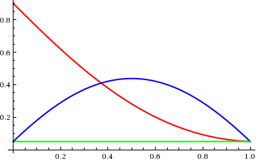
(a) Probability

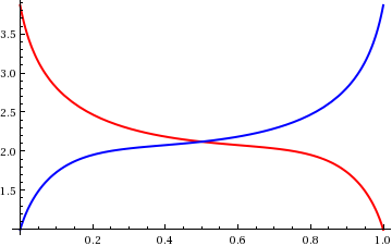
(b) Current velocity

Figure 2: Numerical solution of the three state process versus time. On the left (2a) the behavior of the occupation probability of the first $m(0,t)$ and the second $m(1,t)$ state. On the right (2b) the current velocity components $V(0,t)$, $V(1,t)$ driving the transition.

The probability of the first state is always decreasing while the probability of the intermediate state has a maximum at $t=0.5$ and then symmetrically decays to match its boundary condition. The constant line corresponds to $0.05$ and is plotted to emphasize the convergence of the two occupation probabilities to the the assigned boundary condition. The optimal controls are fast varying near the boundaries while varying more slowly in the bulk of the control horizon. This is the characteristic behavior of optimal controls of thermodynamics functionals described in ScSe07 ; EsKaLiBr10 ; AuMeMG11 ; AuMeMG12 ; AuGaMeMoMG12 . Since the Gibbs entropy vanishes for this symmetric transition the heat release coincides with the entropy production. The numerical evaluation of (60) for the three state system then yields

$$\beta\mathcal{Q}_{\star}=\mathcal{S}_{\star}=4.096$$ (96)

7 Conclusions

We have shown that if the traffic is constrained to a constant value the driving function governing the transition between two states with minimal heat release in a finite time horizon obeys Hamilton-Jacobi-Bellman type equations. The corresponding dynamics is short-ranged as it permits only jumps to nearest-neighbor sites. Our results are the counter-part for Markov jump processes of the entropy bounds derived in AuGaMeMoMG12 for the Langevin dynamics. In this sense, they can also be regarded as refinement of second law of thermodynamics for Markov jump processes. We have also shown that entropy production is not convex in the traffic. As a consequence, interpreting traffic as a control parameter results into singular optimal control strategy. This means that any eventual heat release occurs in a zero Lebesgue measure time interval. It is worth noticing here that jump protocols solutions survive also in the Langevin continuum limit. Namely, if we express as in AuMeMG12 the heat functional in terms of the current velocity it is readily seen that the lower bound provided by the variation of the Gibbs-Shannon entropy becomes tight for a jump protocol for which the current velocity is vanishing throughout the control horizon. This latter condition then just means that the drift must remain in equilibrium so that the resulting protocol is precisely the one found here in the case of unconstrained traffic. In the Langevin case, this kind of solutions for the heat functional can be ruled out a-priori by restricting admissible control to smooth diffusions. The current velocity representation also evinces the subtle problems in which we incur when turning to thermodynamic work minimization. For the work it is not possible to find a minimizer by restricting admissible protocols to smooth diffusions because of the non-coercive functional dependence on the control occasioned by the boundary cost term specified by the internal energy variation. Justifying in which sense variations for fixed terminal value of the internal energy may still define to an optimality criterion for a cost functional compatible with the interpretation of non-equilibrium thermodynamic work calls then for a more refined analysis such as that carried out in AuMeMG12 . An comprehensive discussion of these results can be found in PMG12 .

To summarize, we can say that the analysis of optimal control of Markov jump process helps to shed further light on the interpretation of the result previously available for the Langevin dynamics. Restricting admissible controls to those determining the driving function provide then a simplified model for the continuous limit Langevin dynamics. Such an approach is particularly beneficial because, as exemplified by the three state jump process, numerical solutions of the Hamilton-Jacobi-Bellman equations become extremely computing time inexpensive in comparison to the Monge-Ampère-Kantorovich scheme solving the Langevin dynamics AuGaMeMoMG12 . Still, the three state Markov jump process captures relevant qualitative features of the Langevin dynamics. The discrete dynamics is therefore very useful for capturing the qualitative features of the optimal control of non-equilibrium thermodynamics statistical indicators, such as higher moments of the heat functional itself, the Hamilton-Jacobi-Bellman equations thereof are not amenable, at least as far as it is currently known, to any fast integration scheme in the Langevin limit.

8 Acknowledgments

It is a pleasure to thank Erik Aurell and Krzysztof Gawȩdzki for many enlightening discussions on optimal control in stochastic thermodynamics. P.M.-G.’s work was supported by the Center of Excellence “Analysis and Dynamics”of the Academy of Finland. The authors gratefully acknowledge support from the European Science Foundation and hospitality of NORDITA where this work has been initiated during their stay within the framework of the ”Non-equilibrium Statistical Mechanics” program. LP acknowledges the support of FARO and of PRIN 2009PYYZM5.

Appendices

Appendix A Mean backward derivative

Local detailed balance (7) ensures that the chain of equalities

$$\mathrm{E}_{\mathtt{x},t+dt}f(\xi_{t})=\sum_{\tilde{\mathtt{x}}\in\mathbb{S}}f(\tilde{\mathtt{x}})\tilde{\mathsf{P}}_{t,t+dt}\left(\tilde{\mathtt{x}}\,|\mathtt{x}\right)$$ (97)

$$=\sum_{\tilde{\mathtt{x}}\in\mathbb{S}}\mathsf{P}_{t+dt,t}\left(\mathtt{x},t+dt\,|\,\tilde{\mathtt{x}},t\right)\tilde{\mathtt{x}}\frac{m(\tilde{\mathtt{x}},t)}{m(\mathtt{x},t+dt)}$$

Expanding in Taylor series, neglecting terms $O(dt^{2})$ and using the Master equations (4), (5) yields the proof of (8).

Appendix B Evaluation of the Kullback-Leibler divergence (15)

The first term on the right hand side of (15) is vanishing on average

$$\mathrm{E}^{(\xi)}\int_{t_{o}}^{t_{f}}dt\,\sum_{\mathtt{x}\in\mathcal{S}}\left[\mathsf{K}_{t}(\mathtt{x}|\xi_{t})-\bar{\mathsf{K}}_{t}(\mathtt{x}|\xi_{t})\right]=$$ (98)

$$\int_{t_{o}}^{t_{f}}dt\,\sum_{\mathtt{x},\mathtt{y}\in\mathcal{S}}\left[\mathsf{K}_{t}(\mathtt{x}|\mathtt{y})-\mathsf{K}_{t}(\mathtt{y}|\mathtt{x})\frac{\mathrm{m}(\mathtt{y},t)}{\mathrm{m}(\mathtt{x},t)}\right]\mathrm{m}(\mathtt{x},t)=0$$

The second addend

$$\mathrm{E}^{(\xi)}\sum_{t\in\mathbb{J}(\xi)}\ln\frac{\mathsf{K}_{t}(\xi_{t}|\xi_{t_{-}})}{\bar{\mathsf{K}}_{t}(\xi_{t}|\xi_{t_{-}})}\equiv\int_{t_{o}}^{t_{f}}dt\sum_{\mathtt{x},\mathtt{y}\in\mathcal{S}}\ln\frac{\mathsf{K}_{t}(\mathtt{x}|\mathtt{y})\,\mathrm{m}(\mathtt{y},t)}{\mathsf{K}_{t}(\mathtt{y}|\mathtt{x})\,\mathrm{m}(\mathtt{x},t)}\mathsf{K}_{t}(\mathtt{x}|\mathtt{y})\mathrm{m}(\mathtt{y},t)$$ (99)

carries two contributions. The first is the Shannon-Gibbs entropy of the transformation

$$\int_{t_{o}}^{t_{f}}dt\sum_{\mathtt{x},\mathtt{y}\in\mathcal{S}}\ln\frac{\mathrm{m}(\mathtt{y},t)}{\mathrm{m}(\mathtt{x},t)}\mathsf{K}_{t}(\mathtt{x}|\mathtt{y})\mathrm{m}(\mathtt{y},t)$$ (100)

$$=\int_{t_{o}}^{t_{f}}dt\sum_{\mathtt{x},\mathtt{y}\in\mathcal{S}}\ln\mathrm{m}(\mathtt{y},t)\,[\mathsf{K}_{t}(\mathtt{x}|\mathtt{y})\,\mathrm{m}(\mathtt{y},t)-\mathsf{K}_{t}(\mathtt{y}|\mathtt{x})\,\mathrm{m}(\mathtt{x},t)]$$

$$=-\int_{t_{o}}^{t_{f}}dt\,\sum_{\mathtt{y}\in\mathcal{S}}\ln\mathrm{m}(\mathtt{y},t)\,\partial_{t}\mathrm{m}(\mathtt{y},t)=-\mathrm{E}^{\xi}\ln\frac{\mathrm{m}_{f}(\xi_{t_{f}})}{\mathrm{m}_{o}(\xi_{t_{o}})}$$

by probability conservation eq. (19). The second specifies the thermodynamic heat and is given in the main text.

Appendix C Alternative treatment of the variational problem

We may state the optimization problem directly for the heat functional using as independent control the reduced traffic and the driving functional $\mathsf{A}$:

$$\beta\,\mathcal{Q}=\int_{t_{o}}^{t_{f}}dt^{\prime}\sum_{\mathtt{x},\tilde{\mathtt{x}}\in\mathcal{S}}\mathsf{A}(\mathtt{x},\tilde{\mathtt{x}},t)\,\mathsf{G}(\mathtt{x},\tilde{\mathtt{x}},t)\,e^{\frac{\mathsf{A}(\mathtt{x},\tilde{\mathtt{x}},t)}{2}}\,m(\tilde{\mathtt{x}},t)$$ (101)

The corresponding value function in such a case is the solution of the backward Kolmogorov equation

$$[(\partial_{t}+\mathsf{L})J](\tilde{\mathtt{x}},t)+\sum_{\mathtt{x}\in\mathbb{S}}\mathsf{A}(\mathtt{x},\tilde{\mathtt{x}},t)\,\mathsf{G}(\mathtt{x},\tilde{\mathtt{x}},t)\,e^{\frac{\mathsf{A}(\mathtt{x},\tilde{\mathtt{x}},t)}{2}}=0$$ (102)

where, as in the main text, we require the variation of $J$ to vanish at $t_{f}$ as we regard $J(\cdot,t_{f})$ as a functional of $m(\cdot,t_{f})$. By Dynkin formula (see e.g. Klebaner ) we must have

$$\beta\,\mathcal{Q}=\sum_{\tilde{\mathtt{x}}}\left\{m(\tilde{x},t_{o})\,J(\tilde{\mathtt{x}},t_{o})-m(\tilde{x},t_{f})\,J(\tilde{\mathtt{x}},t_{f})\right\}$$ (103)

whence using the boundary conditions ti follows that

$$\beta\,\mathcal{Q}^{\prime}=\sum_{\tilde{\mathtt{x}}}m(\tilde{x},t_{o})\,J^{\prime}(\tilde{\mathtt{x}},t_{o})$$ (104)

The weak sense variation of (102) yields the conditions

$$0=J(\mathtt{x},t)-J(\tilde{\mathtt{x}},t)+\mathsf{A}(\mathtt{x},\tilde{\mathtt{x}},t)$$ (105a)

$$0=\left\{m(\mathtt{x},t)\,e^{\frac{\mathsf{A}(\mathtt{x},\tilde{\mathtt{x}},t)}{2}}\ +m(\tilde{\mathtt{x}},t)\,e^{-\frac{\mathsf{A}(\mathtt{x},\tilde{\mathtt{x}},t)}{2}}\right\}\,\frac{J(\mathtt{x},t)-J(\tilde{\mathtt{x}},t)}{2}$$ (105b)

$$+\left\{e^{\frac{\mathsf{A}(\mathtt{x},\tilde{\mathtt{x}},t)}{2}}\,m(\tilde{\mathtt{x}},t)-\,e^{-\frac{\mathsf{A}(\mathtt{x},\tilde{\mathtt{x}},t)}{2}}\,m(\mathtt{x},t)\right\}$$

$$+\frac{\mathsf{A}(\mathtt{x},\tilde{\mathtt{x}},t)}{2}\left\{e^{\frac{\mathsf{A}(\mathtt{x},\tilde{\mathtt{x}},t)}{2}}\,m(\tilde{\mathtt{x}},t)+\,e^{-\frac{\mathsf{A}(\mathtt{x},\tilde{\mathtt{x}},t)}{2}}\,m(\mathtt{x},t)\right\}$$

Upon inserting the Ansatz

$$\mathsf{A}(\mathtt{x},\tilde{\mathtt{x}},t)=\mathsf{F}(\mathtt{x},\tilde{\mathtt{x}},t)+\ln m(\mathtt{x},t)-\ln m(\tilde{\mathtt{x}},t)$$ (106a)

$$J(x,t)=B(x,t)-\ln m(\mathtt{x},t)$$ (106b)

we recover the stationary point equations (52).

References

• (1) A. Alemany, M. Ribezzi, and F. Ritort. Recent progress in fluctuation theorems and free energy recovery. AIP Conference Proceedings, 1332(1):96–110, 2011, arXiv:1101.3174.
• (2) E. Aurell, K. Gawȩdzki, C. Mejía-Monasterio, R. Mohayaee, and P. Muratore-Ginanneschi. Refined Second Law of Thermodynamics for fast random processes. Journal of Statistical Physics, 147(3):487–505, April 2012, arXiv:1201.3207.
• (3) E. Aurell, C. Mejía-Monasterio, and P. Muratore-Ginanneschi. Optimal protocols and optimal transport in stochastic thermodynamics. Physical Review Letters, 106(25):250601, June 2011, arXiv:1012.2037.
• (4) E. Aurell, C. Mejía-Monasterio, and P. Muratore-Ginanneschi. Boundary layers in stochastic thermodynamics. Physical Review E, 85(2):020103(R), Februray 2012, arXiv:1111.2876.
• (5) A. Bérut, A. Arakelyan, A. Petrosyan, S. Ciliberto, R. Dillenschneider, and E. Lutz. Experimental verification of Landauer’s principle linking information and thermodynamics. Nature, 483:187–189, March 2012.
• (6) D. M. Carberry, J. C. Reid, G. M. Wang, E. M. Sevick, D. J. Searles, and D. J. Evans. Fluctuations and irreversibility: an experimental demonstration of a second-law-like theorem using a colloidal particle held in an optical trap. Physical Review Letters, 92:140601, 2004.
• (7) R. Chétrite and K. Gawȩdzki. Fluctuation relations for diffusion processes. Communications in Mathematical Physics, 282:469–518, 2007, arXiv:0707.2725.
• (8) R. Chétrite and S. Gupta. Two refreshing views of Fluctuation Theorems through Kinematics Elements and Exponential Martingale. Journal of Statistical Physics, 143:543–584, 2011, arXiv:1009.0707.
• (9) D. Collin, F. Ritort, C. Jarzynski, S. B. Smith, J. Ignacio Tinoco, and C. Bustamante. Verification of the Crooks fluctuation theorem and recovery of RNA folding free energies. Nature, 437(7056):231–234, Sep 2005.
• (10) G. E. Crooks. Path-ensemble averages in systems driven far from equilibrium. Physical Review E, 61(3):2361–2366, March 2000, arXiv:cond-mat/9908420.
• (11) M. Davis and R. Elliott. Optimal control of a jump process. Probability Theory and Related Fields, 40:183–202, 1977. 10.1007/BF00736046.
• (12) M. Esposito, R. Kawai, K. Lindenberg, and C. van den Broeck. Finite-time thermodynamics for a single-level quantum dot. Europhysics Letters Volume 89 Number 2, 89(2):20003, February 2010, arXiv:0909.3618.
• (13) M. Esposito and C. van den Broeck. Three Detailed Fluctuation Theorems. Physical Review Letters, 104(9):090601, March 2010, arXiv:0911.2666.
• (14) M. Esposito and C. van den Broeck. Second law and Landauer principle far from equilibrium. Europhysics Letters, 95:40004, August 2011.
• (15) D. J. Evans, E. G. D. Cohen, and G. P. Morriss. Probability of second law violations in shearing steady states. Physical Review Letters, 71:2401–2404, Oct 1993.
• (16) D. J. Evans and D. J. Searles. Equilibrium microstates which generate second law violating steady states. Physical Review E, 50(2):1645–1648, August 1994.
• (17) W. H. Fleming and M. H. Soner. Controlled Markov processes and viscosity solutions, volume 25 of Stochastic modelling and applied probability. Springer, 2nd, revised edition, 2006.
• (18) G. Gallavotti and E. G. D. Cohen. Dynamical Ensembles in Nonequilibrium Statistical Mechanics. Physical Review Letters, 74(14):2694–2697, April 1995, arXiv:chao-dyn/9410007.
• (19) K. Gawȩdzki. Relations de Fluctuations et Dissipations (aspect theoriques). ENS Lyons, Lecture Notes (2011), 2011.
• (20) J. R. Gomez-Solano, A. Petrosyan, S. Ciliberto, R. Chétrite, and K. Gawȩdzki. Experimental Verification of a Modified Fluctuation-Dissipation Relation for a Micron-Sized Particle in a Nonequilibrium Steady State. Physical Review Letters, 103(4):040601, July 2009.
• (21) F. Guerra and L. M. Morato. Quantization of dynamical systems and stochastic control theory. Physical Review D, 27(8):1774–1786, Apr 1983.
• (22) T. Hatano and S.-i. Sasa. Steady-state thermodynamics of Langevin systems. Physical Review Letters, 86(16):3463–3466, April 2001, arXiv:cond-mat/0010405.
• (23) A. Imparato and L. Peliti. The distribution function of entropy flow in stochastic systems. Journal of Statistical Mechanics: Theory and Experiment, 2007:L02001, February 2007, arXiv:cond-mat/0611078.
• (24) C. Jarzynski. Nonequilibrium Equality for Free Energy Differences. Physical Review Letters, 78(14):2690–2693, April 1997, arXiv:cond-mat/9610209.
• (25) S. Katz, J. L. Lebowitz, and H. Spohn. Nonequilibrium steady states of stochastic lattice gas models of fast ionic conductors. Journal of Statistical Physics, 34:497–537, 1984.
• (26) C. Kipnis and C. Landim. Scaling Limits of Interacting Particle Systems. Number 320 in Grundlheren der Mathematischen Wissenschaften. Springer, 1999.
• (27) F. C. Klebaner. Introduction to stochastic calculus with applications. Imperial College Press, 2 edition, 2005.
• (28) A. N. Kolmogorov. Zur Theorie der Markoffschen Ketten. Mathematische Annalen, 112(1):155–160, 1936.
• (29) T. Konstantopoulos, Z. Zerakidze, and G. Sokhadze. Radon-nikodym theorem. In M. Lovric, editor, International Encyclopedia of Statistical Science, pages 1161–1164. Springer Berlin Heidelberg, 2011.
• (30) S. Kullback and R. Leibler. On Information and Sufficiency. Annals of Mathematical Statistics, 22(1):79–86, 1951.
• (31) J. Kurchan. Fluctuation theorem for stochastic dynamics. Journal of Physics A: Mathematical and General, 31(16):3719, April 1998, arXiv:cond-mat/9709304.
• (32) J. L. Lebowitz and H. Spohn. A Gallavotti-Cohen Type Symmetry in the Large Deviation Functional for Stochastic Dynamics. Journal of Statistical Physics, 95(1):333–365, March 1999, arXiv:cond-mat/9811220.
• (33) J. Liphardt, S. Dumont, S. B. Smith, J. Ignacio Tinoco, and C. Bustamante. Equilibrium Information from Nonequilibrium Measurements in an Experimental Test of Jarzynski’s Equality. Science, 7:1832–1835, June 2002.
• (34) C. Maes, K. Netočný, and B. Wynants. On and beyond Entropy Production: the Case of Markov Jump Processes. Markov Processes and Related Fields, 14(3):445–464, 2008, arXiv:0709.4327.
• (35) C. Maes, F. Redig, and A. V. Moffaert. On the definition of entropy production, via examples. Journal of Mathematical Physics, 41(3):1528–1554, March 2000.
• (36) P. Muratore-Ginanneschi. On the use of stochastic differential geometry for non-equilibrium thermodynamics modeling and control. arXiv preprint, October 2012, arXiv:1210.1133.
• (37) M. Nagasawa. Time reversions of Markov processes. Nagoya Mathematical Journal, 24:177–204., 1964.
• (38) E. Nelson. Dynamical Theories of Brownian Motion. Princeton University Press, second edition edition, 2001.
• (39) S. R. Pliska. Controlled jump processes. Stochastic Processes and their Applications, 3(3):259 – 282, 1975.
• (40) F. Ritort. Nonequilibrium Fluctuations in Small Systems: From Physics to Biology. In S. A. Rice, editor, Advances in Chemical Physics, volume 137. John Wiley & Sons,, April 2008.
• (41) T. Schmiedl and U. Seifert. Optimal Finite-Time Processes In Stochastic Thermodynamics. Physical Review Letters, 98(10):108301, March 2007, arXiv:cond-mat/0701554.
• (42) U. Seifert. Entropy Production along a Stochastic Trajectory and an Integral Fluctuation Theorem. Physical Review Letters, 040602(4):95, July 2005, arXiv:cond-mat/0503686.
• (43) E. H. Trepagnier, C. Jarzynski, F. Ritort, G. E. Crooks, C. J. Bustamante, and J. Liphardt. Experimental test of Hatano and Sasa’s nonequilibrium steady-state equality. Proceedings of the National Academy of Sciences, 101:15038–15041, 2004.
• (44) R. van Handel. Stochastic calculus and stochastic control. Lecture Notes, Caltech, 2007.
• (45) C. Villani. Optimal transport: old and new, volume 338 of Grundlehren der mathematischen Wissenschaften. Springer, 2009.
• (46) G. M. Wang, E. M. Sevick, E. Mittag, D. J. Searles, and D. J. Evans. Experimental Demonstration of Violations of the Second Law of Thermodynamics for Small Systems and Short Time Scales. Physical Review Letters, 89(5):050601, July 2002.
• (47) I. Wolfram Research. Mathematica. Wolfram Research, Inc., 1991–2010.
• (48) J.-C. Zambrini. Variational processes and stochastic versions of mechanics. Journal of Mathematical Physics, 27(9):2307–2330, 1986.