Two refreshing views of Fluctuation Theorems through Kinematics Elements and Exponential Martingale

Abstract

In the context of Markov evolution, we present two original approaches to obtain Generalized Fluctuation-Dissipation Theorems (GFDT), by using the language of stochastic derivatives and by using a family of exponential martingales functionals. We show that GFDT are perturbative versions of relations verified by these exponential martingales. Along the way, we prove GFDT and Fluctuation Relations (FR) for general Markov processes, beyond the usual proof for diffusion and pure jump processes. Finally, we relate the FR to a family of backward and forward exponential martingales.

1 Introduction

One of the cornerstones of statistical physics is the Fluctuation-Dissipation Theorem (FDT) Call1 ; Kubo0 ; MPRV ; Risk , whereby, for equilibrium systems, response to a small perturbation of the Hamiltonian is related to dynamical correlation. This theorem rationalizes the famous regression principle of Onsager Ons1 ; Ons2 : the decay of spontaneous fluctuation cannot be distinguished from the decay of forced fluctuation. More precisely, suppose we perturb a system in equilibrium at temperature $T$ by adding to its time-independent Hamiltonian $H$ a small time-dependent term, such that $H\rightarrow H-k_{t}O$. Here, $O$ is an observable and $k_{t}$ is a real function. Throughout this paper, we measure temperatures in units of the Boltzmann constant $k_{B}$. The FDT asserts that the response of an observable $O^{\prime}$ is related to the two-time correlation function as

$$T\left.\frac{\delta\left\langle O^{\prime}_{t}\right\rangle^{\prime}}{\delta k_{s}}\right|_{k=0}=\partial_{s}\left\langle O_{s}O^{\prime}_{t}\right\rangle,$$ (1)

with $t\geq s$. In this relation, the brackets, $\left\langle{\ }\right\rangle$ and $\left\langle{\ }\right\rangle^{\prime}$, denote expectation in the unperturbed and perturbed processes, respectively. Since mid-nineties, this theorem has been extended to nonequilibrium systems in two related directions. The first is the discovery of various Fluctuation Relations (FR) Crooks2 ; Eva ; Gal ; Jarz , the so-called Gallavotti-Cohen relation Eva ; Gal , the Jarzynski equality Jarz and the Crooks theorem Crooks2 . All of these hold arbitrarily far from equilibrium and can be viewed as non-perturbative extensions Gall2 of the FDT (1). These relations constrain the distribution of entropy production or work performed in the system. The second is the extension of the relation (1) between response and correlation in the linear response regime to nonequilibrium states (stationary as well as non-stationary), for example, those in glassy systems and soft spin models Cri1 ; Cug1 ; Die1 ; Lip1 ; May1 and also in relation to broken supersymmetry Zim1 . This second direction has seen an upsurge in the last three years through formulation of the Generalized Fluctuation-Dissipation Theorems ( GFDT), mainly in the works of Seifert and Speck in Stuttgart Sei2 ; SpS0 ; Spe2 , Baiesi, Maes and Wynants in Leuven Bae1 ; Bae2 ; Mae3 , and Gawedzki and Chetrite in Lyon and Falkovich in Rehovot Fal2 ; Che3 ; Che4 (see, also, the works Liu2 ; Pro1 ). Moreover, experimental verifications of the GFDT on colloidal particle have been done in Lyon Gom1 ; Gom2 .

In the present paper, we revisit, generalize, and unify these FR and GFDT by couching them in the language of the kinematics of a general Markov process, without strict mathematical rigor. We show that this language allows elementary proofs and generalizations of the different GFDT which exist in the literature. We also consider a new family of non-perturbative extensions of the GFDT which concerns a so-called exponential forward martingale functionals Chu1 ; Rev1 ; Pal1 . Finally, we revisit the FR and show their relation to forward and backward exponential martingales. In the process, we prove that a certain version of the Crooks theorem and the Jarzynski equality hold for fairly general Markov processes, whereas the Gallavotti-Cohen relation for the performed work can be violated when the particle is subjected to a Poisson or Levy noise Bau1 ; Tou1 .

General Markov stochastic processes form an integral part of modeling of dynamics in statistical mechanics. Although largely idealized, they often provide a sufficiently realistic description of experimental situations and have traditionally served as a playground for both theoretical considerations and numerical studies. In a continuous space (e.g., $\mathcal{R}^{d}$), all continuous time Markov processes consist of some combinations of diffusion, deterministic motion and random jumps. Markov processes corresponding to equilibrium dynamics are characterized by the detailed balance property which ensures that the net probability flux between microstates of the system vanishes. On the other hand, with nonequilibrium Markov dynamics, detailed balance is violated and there are non-zero probability fluxes even in a stationary situation. For the purpose of characterizing the difference between equilibrium and nonequilibrium dynamics, it is interesting to find a vector field, a kind of velocity, which vanishes in equilibrium. Such an object was introduced in the sixties by Nelson in his seminal work Nel with the notion of current velocity that we call here the local symmetric velocity. This quantity is an average of a well-chosen instantaneous velocity of the process conditioned to pass through a given point. It was shown in Che4 that nonequilibrium diffusive dynamics (without the random jumps) takes, in the Lagrangian frame of this velocity, an equilibrium form with the detailed balance property and this explains the usual form (1) of the FDT in that frame, which was observed previously in Fal2 . The issue regarding the extension of this result to other types of Markov processes is addressed in this article in one of the Sections.

The formulation of the usual FDT (1) for some Markov processes is known since long time Call1 ; Kubo0 ; Risk in physics, but now it has a strictly mathematically rigorous formulation Dem1 . For the FR, shortly after the earliest articles in the context of deterministic dynamics Eva ; Gal , the fluctuation relations were proved for some Markovian dynamics. In Jarz2 , Jarzynski generalized his relation to time-dependent pure jump Markov processes. At around the same time, Kurchan showed in Kurchan that the stationary FR hold for the stochastic Langevin-Kramers evolution with additive noise. His result was extended to more general diffusion processes by Lebowitz and Spohn in LebowSp . In Maes , Maes has traced the origin of FR to the Gibbsian nature of the statistics of the dynamical histories. Finally, these relations were put into the language of stochastic thermodynamics by Sekimoto Sek and Seifert Sei . There exist now many reviews on fluctuation relations in the Markovian context, like Sch1 ; Jia1 ; Liu3 for pure jump process or CHCHJAR ; Che1 ; Kurchan2 ; Jia1 ; Liu1 for diffusion process, but the extension to FR for general Markov process is still under debate Bau1 ; Tou1 .

The paper consists of seven Sections and six Appendices. Section 2 sets the stage and provides notations by briefly stating definitions relevant to Markov processes. In particular, in Section 2.1, we recall the notions of transition probability, Markov generator, stationary state and equilibrium state. In Section 2.2, we introduce the notion of cotransition probability, cogenerator, current and velocity operator . We also elucidate the relation between these objects. Section 3 develops the kinematics of a Markov process Nel by defining a set of local derivatives and local velocities associated with such processes. It is proved in Section 3.2 that these local derivatives appear naturally in the time derivative of correlation function which appears on the right hand side of the FDT (1). Section 4 investigates the form of the kinematics elements, local velocities and velocity operator, for the three most common examples of Markov process which appear in physics. First is the pure jump process in Section 4.1, which is a process with no diffusion and deterministic evolution. Second is the diffusion process, considered in Section 4.2, which is a process that, on the contrary, neglects the random jumps. Finally, in Section 4.3, we investigate the less considered case which mixes diffusion, random jumps and deterministic motion given by a stochastic equation with Gaussian and Poissonian white noises. The latter noise consists of a sequence of $\delta$-function shaped pulses with random heights occurring at randomly distributed times. Such a noise appears in the physical world, for example, it describes the emission of electrons in diodes or the counting process of photons. As examples, we study two physical realizations of such a dynamics involving colloidal particles trapped on the unit circle. It turns out that analytical computation of the stationary density is possible only for the first realization, and not for the second. Hence, we resort to extensive numerical simulations to obtain the stationary density as well as the local velocity for the second realization.

The first central section which contains novel results is Section 5 which is devoted to the study of the behavior of a Markovian system under a perturbation. More precisely, Section 5.1 recalls the notion of response function to an arbitrary perturbation. Section 5.2 introduces a special family of perturbations, which we call Hamiltonian ones or generalized Doob $h$-transforms. These include the usual perturbations considered in the physics literature. Section 5.3 proves in a very simple way, thanks to the language of kinematics elements, that the recent GFDT Bae1 ; Bae2 ; Fal2 ; Che3 ; Che4 ; Gom1 ; Liu2 ; Mae3 ; Pro1 ; Sei2 ; SpS0 ; Spe2 are obtained in this general Markovian context for the case of a Hamiltonian perturbation. We also numerically verify the GFDT in the context of the example of Section 4.3.2 involving stochastic dynamics with Gaussian and Poissonian white noise. Section 5.4 presents the GFDT which result from a more general class of perturbations, such as a time change Dem1 or a thermal perturbation pulse Che4 ; Risk . The second crucial section is Section 6. Here, we present global (non-perturbative) versions of these GFDT which involve a family of functionals called exponential martingales in the probability literature Pal1 . Originally, a martingale referred to a class of betting strategies, but this notion has now become central to the modern probability theory and characterizes, ironically, a model of a fair game. A martingale is process whose expectation in the future, given the knowledge accumulated up to now, is its present value Chu1 ; Doo1 ; Fel1 ; Rev1 ; Str . In Section 6.1, we present a family of exponential martingales, which are natural objects associated with the Hamiltonian perturbations because they are the ratio of the trajectory measures of the perturbed and the unperturbed processes. Moreover, we prove in Section 6.1.3 that they also provide global versions of the GFDT. Finally, in Section 6.2, we revisit, in the light of the martingale theory, the usual FR for quite general Markov processes and underline the relation with the previously considered exponential martingales. In particular, this rationalizes the typical martingale form $\left\langle\exp\left(-W\right)\right\rangle=1$ of the Jarzynski equality. Section 7 presents our conclusions. The Appendices collect some simple but technical arguments.

2 Elements of a Markov process

As mentioned in the introduction, our study deals with nonequilibrium systems modeled by Markov processes. We begin by recollecting below some basic properties of a Markov process App ; Blu1 ; Chu1 ; Doo1 ; Fel1 ; Rev1 ; Str . We consider a continuous time Markov process $\mathbf{x}_{t}$ which takes values in a space $\mathcal{E}$. The space $\mathcal{E}$ could, for example, be $\mathcal{R}^{d}$ or a counting space.

2.1 Transition probability, stationary state and equilibrium

The dynamics of the process is given by a family of transition functions $P_{s}^{t}(x,dy)$ which satisfy the Chapmann-Kolmogorov rule:

$$\int P_{s}^{u}(x,dy)P_{u}^{t}(y,dz)=P_{s}^{t}(x,dz)~{}~{}~{}~{}~{}~{}~{}~{}\forall~{}~{}s\leq u\leq t,$$ (2)

where $P_{s}^{u}(x,dy)$ is the probability that the process has the value $\left[y,y+dy\right]$ at time $u$, conditioned on the fact that it had the value $x$ at time $s$. Here, and in the following, the notation $dy$ represents the Lebesgue measure or the counting measure, depending on $\mathcal{E}$. We will assume for simplicity that the transition functions and all other relevant functions admit a density with respect to this measure (i.e., $P_{s}^{t}(x,dy)=P_{s}^{t}(x,y)dy)$. Moreover, we consider processes without death or explosion, i.e., with so-called honest transition probabilities, such that one has the normalization condition $\int dyP_{s}^{t}(x,y)=1$. This could be easily achieved in general, e.g., by enlarging the space to include a coffin state. It will be useful to think of the transition functions as linear operators $P_{s}^{t}$ which form an inhomogeneous semi-group, and which are defined by their action on a bounded function $f$ in $\mathcal{E}$ in the following way:

$$P_{s}^{t}[f](x)\equiv\int dyP_{s}^{t}(x,y)f(y).$$ (3)

The family of transition functions of a Markov process which can be written down explicitly is very restrictive. Hence, it is more practical to define the generator $L_{t}$ of this inhomogeneous semi-group, under appropriate regularity conditions Chu1 ; Rev1 , by the following equation:

$$P_{s}^{t}=\overrightarrow{\exp}\left(\int_{s}^{t}L_{u}\,du\right)\equiv\sum_{n}\int_{s\leq s_{1}\leq s_{2}\leq\ldots\leq s_{n}\leq t}\prod_{i=1}^{n}ds_{i}L_{s_{1}}\circ L_{s_{2}}\circ\ldots\circ L_{s_{n}}.$$ (4)

This equation is equivalent to the forward and backward Kolmogorov equation, given, respectively, by

$$\partial_{t}P_{s}^{t}=P_{s}^{t}\circ L_{t},\text{ \ \ and \ }\partial_{s}P_{s}^{t}=-L_{s}\circ P_{s}^{t}.$$ (5)

Here, the symbol $\circ$ means composition of operators. Also, the initial condition is $P_{s}^{s}=\mathcal{I}$. For the transition function to be honest, the generator must obey $L_{t}[1]=0$, where $1$ is the function which is equal to $1$ on $\mathcal{E.}$ If the initial measure of the process is $\mu_{0}(dx)=\rho_{0}(x)dx$, we may define the averages of a functional of the process $\mathbf{x}$ as

$$\left\langle F\right\rangle\equiv\int\mu_{0}(dx)\mathbf{E}_{t_{0},x}\left(F[x]\right),$$ (6)

where $\mathbf{E}_{t_{0},x}$ stands for the expectation of the functional of the process $\mathbf{x}$ with the initial condition $x_{t_{0}}=x$. Next, it will be useful to define a path measure $M_{\mu_{0},\left[s,t\right]}[dx]\equiv dM_{\mu_{0},\left[s,t\right]}[x]$ on the space of trajectories by the following equation:

$$\left\langle F\right\rangle\ =\ \int F[x]\,M_{\mu_{0},\left[s,t\right]}[dx],$$ (7)

where $F$ is a functional of the path from time $s$ to time $t$. The instantaneous (or single time) probability density function (PDF) of the process is given by

$$\rho_{t}(x)=\left\langle\delta(x_{t}-x)\right\rangle.$$ (8)

Its time evolution may be deduced from (5). We obtain the following Fokker-Planck equation:

$$\partial_{t}\rho_{t}=L_{t}^{\dagger}[\rho_{t}],$$ (9)

where $L_{t}^{\dagger}$ is the formal adjoint of $L_{t}$ with respect to the Lebesgue (or counting) measure. A stationary state ($\rho_{t}\equiv\rho$) then satisfies the equation

$$L_{t}^{\dagger}[\rho]=0.$$ (10)

Further, one says that the process is in equilibrium, i.e., it satisfies the infinitesimal detailed balance relation if the following condition for the generator is satisfied :

$$\rho\circ L_{t}\circ\rho^{-1}=L_{t}^{\dagger}.$$ (11)

If the process is time-homogeneous, the above equation is equivalent to the usual detailed balance condition for the transition function:

$$\rho(x)P_{t-s}(x,y)=\rho(y)P_{t-s}(y,x).$$ (12)

It will be useful to define two particular families of non-stationary states. First, one defines the so-called accompanying density $\pi_{t}$ which satisfies the instantaneous relation Han ; Jarz2

$$\ L_{t}^{\dagger}[\pi_{t}]=0.$$ (13)

Next, we introduce the subclass of accompanying density, that we assume to be in local detailed balance, such that the generator verifies the instantaneous time-dependent version of the relation (11):

$$\pi_{t}\circ L_{t}\circ\pi_{t}^{-1}=L_{t}^{\dagger}.$$ (14)

2.2 Cotransition probability, current and velocity operator.

The two-point density $\left\langle\delta\left(x_{s}-x\right)\delta\left(x_{t}-y\right)\right\rangle$ of a Markov process is usually expressed by conditioning with respect to the earlier time $s$, as

$$\left\langle\delta\left(x_{s}-x\right)\delta\left(x_{t}-y\right)\right\rangle=\rho_{s}(x)P_{s}^{t}(x,y).$$ (15)

It can also be expressed by conditioning with respect to the later time $t$ in terms of the so-called cotransition probability $P_{s}^{\ast t}$ Dyn1 (sometimes called the backward transition probability Dyn2 ; Nel2 ) as

$$\left\langle\delta\left(x_{s}-x\right)\delta\left(x_{t}-y\right)\right\rangle=P_{s}^{\ast t}(x,y)\rho_{t}(y).$$ (16)

This cotransition probability satisfies the Chapman-Kolmogorov equation (2), but the normalization condition becomes $\int dxP_{s}^{\ast t}(x,y)=1.$ The relation between the transition and the cotransition probability can then be expressed by the operator formula $P_{s}^{\ast t}=\rho_{s}\circ P_{s}^{t}\circ\rho_{t}^{-1}$, which implies the forward equation

$$\partial_{t}P_{s}^{\ast t}=P_{s}^{\ast t}\left(\rho_{t}\circ L_{t}\circ\rho_{t}^{-1}-\rho_{t}^{-1}\left(\partial_{t}\rho_{t}\right)\right).$$ (17)

We will now introduce a family of operators $L_{t}^{\ast}$, which we call cogenerators, by the following equation:

$$L_{t}^{\ast}=\rho_{t}^{-1}\circ L_{t}^{\dagger}\circ\rho_{t}-\rho_{t}^{-1}\left(\partial_{t}.\rho_{t}\right)\mathcal{I=}\rho_{t}^{-1}\circ L_{t}^{\dagger}\circ\rho_{t}-\rho_{t}^{-1}L_{t}^{\dagger}[\rho_{t}]\mathcal{I},$$ (18)

where $\mathcal{I}$ is the identity kernel, so that the cotransition probability now takes the operatorial form

$$P_{s}^{\ast t}\equiv\overrightarrow{\exp}\left(\int_{s}^{t}du\left(L_{u}^{\ast}\right)^{\dagger}\right).$$ (19)

Then, the property $\int dxP_{s}^{\ast t}(x,y)=1$ is equivalent, as before, to $L_{t}^{\ast}[1]=0$. For a stationary process (10 ), the cogenerator takes the form $L_{t}^{\ast}=\rho^{-1}\circ L_{t}^{\dagger}\circ\rho$, which is the adjoint of $L_{t}$ with respect to the scalar product with weight $\rho$. It is also interesting to associate a current operator and a velocity operator (which depend  on the initial density) with the density $\rho_{t}$ by the following equations:

$$J_{t}\equiv\rho_{t}\circ L_{t}-L_{t}^{\dagger}\circ\rho_{t}\text{ \ and \ }V_{t}\equiv L_{t}-\rho_{t}^{-1}\circ L_{t}^{\dagger}\circ\rho_{t}.$$ (20)

The Fokker-Planck equation (9) can be expressed as

$$\partial_{t}\rho_{t}+J_{t}[1]=0\text{, \ or, equivalently, \ }\partial_{t}\rho_{t}+\rho_{t}V_{t}[1]=0.$$ (21)

The condition (10) for the density $\rho$ to be stationary can then be expressed as

$$J_{t}[1]=0\text{, \ or, equivalently, \ }V_{t}[1]=0.$$ (22)

Otherwise, the equilibrium condition (11) becomes

$$J_{t}=0\text{, \ or, equivalently, \ }V_{t}=0.$$ (23)

Finally, using (9,18,20), we can express the cogenerator in terms of the velocity operator as

$$L_{t}^{\ast}=L_{t}-V_{t}+V_{t}[1]\mathcal{I.}$$ (24)

Then, by (24), equilibrium implies $L_{t}^{\ast}=L_{t}$ . The converse of this statement is true because the condition $L_{t}^{\ast}=L_{t}$ implies that for any function $f$, one has $L_{t}^{\dagger}\left[\rho_{t}f\right]-fL_{t}^{\dagger}\left[\rho_{t}\right]=\rho_{t}L_{t}\left[f\right]$. Then, on integrating by parts over all space, we get
$\int dx\left(-2f(x)L_{t}^{\dagger}\left[\rho_{t}\right](x)\right)=0$, which implies that $L_{t}^{\dagger}\left[\rho_{t}\right]=0$, and then $\rho_{t}=\rho$. Finally, the condition $L_{t}^{\ast}=L_{t}$ can be rewritten as the equilibrium condition.

Figure 1 illustrates these relations between stationarity, equilibrium and the condition of equality between the generator and the cogenerator.

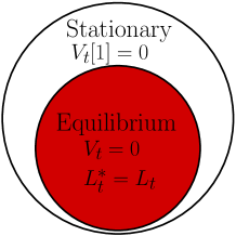
Figure 1: The figure illustrates the relation between stationarity, equilibrium and the condition $L_{t}^{\ast}=L_{t}$, as discussed in the text.

3 Kinematics of a Markov process

The notion of the velocity operator (20) introduced in the last section is quite different from the usual notion of velocity as the derivative of the position. Assume that we want to describe the “naive” kinematics of a general Markov process. The first difficulty is that the trajectories in general are non-differentiable (as in a diffusion process) or, worse, discontinuous (as in a jump process). This does not allow for a straightforward definition of a velocity. In the sixties, Nelson circumvented this difficulty by introducing the notion of forward and backward stochastic derivatives in his seminal work concerning diffusion process with additive noise Nel . Here, we will reproduce the definition of Nelson for a general Markov process. In the following, we assume existence conditions on various quantities, with the expectation that these conditions have already been, or, can be established by rigorous mathematical studies.

3.1 Stochastic derivatives, local velocity

According to Nelson, a Markov process is said to be mean-forward differentiable if the limit $\frac{\lim_{h\rightarrow 0}\left\langle\frac{x_{t+h}-x_{t}}{h}\delta(x_{t}-x)\right\rangle}{\left\langle\delta(x_{t}-x)\right\rangle}$ exists. In this case, this ratio defines the local forward velocity for a process conditioned to be in $x$ at time $t$:

$$v_{t}^{+}(x)\equiv\frac{\lim_{h\rightarrow 0}\left\langle\frac{x_{t+h}-x_{t}}{h}\delta(x_{t}-x)\right\rangle}{\left\langle\delta(x_{t}-x)\right\rangle}.$$ (25)

Similarly, the local backward velocity is defined as

$$v_{t}^{-}(x)\equiv\frac{\lim_{h\rightarrow 0}\left\langle\frac{x_{t}-x_{t-h}}{h}\delta(x_{t}-x)\right\rangle}{\left\langle\delta(x_{t}-x)\right\rangle}.$$ (26)

The local symmetric velocity and the local osmotic velocity are defined as

$$v_{t}(x)\equiv\frac{v_{t}^{+}(x)+v_{t}^{-}(x)}{2}\text{ \ and \ }o_{t}(x)\equiv\frac{v_{t}^{+}(x)-v_{t}^{-}(x)}{2}.$$ (27)

In the same spirit, he defined the stochastic forward, backward and symmetric derivatives of function $f_{t}(x_{t})$ of the process as

$$\left\{\begin{array}[]{c}\frac{d_{+}f}{dt}(x)\equiv\frac{\lim_{h\rightarrow 0}\left\langle\frac{f(t+h,x_{t+h})-f(t,x_{t})}{h}\delta(x_{t}-x)\right\rangle}{\left\langle\delta(x_{t}-x)\right\rangle},\\ \frac{d_{-}f}{dt}(x)\equiv\frac{\lim_{h\rightarrow 0}\left\langle\frac{f(t,x_{t})-f(t-h,x_{t-h})}{h}\delta(x_{t}-x)\right\rangle}{\left\langle\delta(x_{t}-x)\right\rangle},\\ \frac{df}{dt}(x)\equiv\frac{\frac{d_{+}f}{dt}(x)+\frac{d_{-}f}{dt}(x)}{2}.\end{array}\right.$$ (28)

Note that the set of forward, backward and symmetric local velocities are just special cases of derivatives of the function $f_{t}(x_{t})=x_{t}.$ With the definition of the forward transition probability and the cotransition probability given in (15) and (16), we can rewrite the above equations as

$$\left\{\begin{array}[]{c}\frac{d_{+}f}{dt}(x)=\lim_{h\rightarrow 0}\frac{1}{h}\int dyP_{t}^{t+h}(x,y)\left(f(t+h,y)-f(t,x)\right),\\ \frac{d_{-}f}{dt}(x)=\lim_{h\rightarrow 0}\frac{1}{h}\int dyP_{t-h}^{\ast t}(y;x)\left(f(t,x)-f(t-h,y)\right).\end{array}\right.$$ (29)

A Taylor expansion of these transition probabilities using (4) and ( 19) gives

$$\frac{d_{+}}{dt}=\partial_{t}+L_{t}\text{ \ \ and \ \ \ }\frac{d_{-}}{dt}=\partial_{t}-L_{t}^{\ast}.$$ (30)

Also, the stochastic symmetric derivative becomes

$$\frac{d}{dt}=\partial_{t}+\frac{L_{t}-L_{t}^{\ast}}{2}.$$ (31)

The expression of the cogenerator from (24) allows us to express the stochastic symmetric derivative in (31) in terms of the velocity operator (20) as

$$\frac{d}{dt}=\partial_{t}+\frac{V_{t}-V_{t}[1]\mathcal{I}}{2}.$$ (32)

Then, for a steady state (22), $\frac{d}{dt}=\partial_{t}+\frac{V_{t}}{2}$.

We can then deduce that, in the equilibrium case, the stochastic symmetric derivative takes the form of the partial time derivative $\frac{d}{dt}=\partial_{t}$, which gives zero while acting on observables which do not depend explicitly on time. The local symmetric velocity , given in (27), now reads

$$v_{t}^{i}(x)=\frac{L_{t}[x]-L_{t}^{\ast}[x]}{2}=\frac{V_{t}[x^{i}]-V_{t}[1]x^{i}}{2},$$ (33)

and then, for a steady state, $v_{t}^{i}(x)=\frac{V_{t}[x^{i}]}{2}$.

It is important to remark that equilibrium ($V=0$) implies vanishing of the local symmetric velocity but the converse of this statement is not true. Figure 2 illustrates the relation between stationarity, equilibrium and vanishing of the local symmetric velocity.

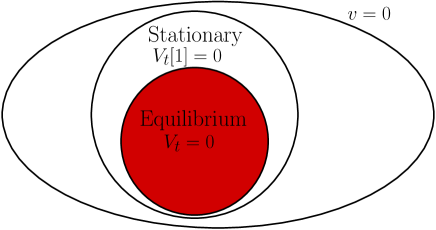
Figure 2: The figure illustrates the relation between stationarity, equilibrium, and vanishing of the local symmetric velocity, as discussed in the text.

One of the authors of the present article proved in Che4 that a diffusion process in the Lagrangian frame of its mean local symmetric velocity takes an equilibrium form, and then the concept of equilibrium and nonequilibrium become closer than usually perceived. However, this property is no longer true for a general process due to the inequivalence between equilibrium and vanishing of the local symmetric velocity.

3.2 Time derivative of two-point correlations

Here we provide useful formulae for the time derivative of the two-time ($s\leq t$) correlation of observables $U$ and $V$ in terms of the correlation of stochastic derivatives (forward or backward) of these observables. The two-point correlation can be expressed in term of the forward transition probability and cotransition probability, (15), (16), as

$$\left\langle U_{s}(x_{s})V_{t}(x_{t})\right\rangle=\int dxdyU_{s}(x)\rho_{s}(x)P_{s}^{t}(x,y)V_{t}(y)=\int dxdyU_{s}(x)P_{s}^{\ast t}(x,y)\rho_{t}(y)V_{t}(y).$$ (34)

We then obtain the formula

$$\partial_{t}\left\langle U_{s}(x_{s})V_{t}(x_{t})\right\rangle=\left\langle U_{s}(x_{s})\frac{d_{+}V_{t}}{dt}(x_{t})\right\rangle\text{ and }\partial_{s}\left\langle U_{s}(x_{s})V_{t}(x_{t})\right\rangle=\left\langle\frac{d_{-}U_{s}}{ds}(x_{s})V_{t}(x_{t})\right\rangle.$$ (35)

The proofs are direct consequence of the definition of transition and cotransition probabilities (4,19) and of forward and backward stochastic derivatives, and are given in Appendix (A). These relations provide motivation for a proof of generalizations of FDT by involving the stochastic derivatives, as discussed later in the paper.

4 Examples of Markov processes

We will now investigate the form of the velocity operator (20 ) and of the local symmetric velocity (33) for the three most popular examples of Markov processes, namely, the pure jump process, the diffusion process and a process generated by a stochastic equation with both Gaussian and Poissonian white noise.

4.1 Pure jump process

Roughly speaking, a Markov process is called a pure jump process (or, a pure discontinuous process) if, after “arriving” into a state, the system stays there for an exponentially-distributed random time interval. It then jumps into another state chosen randomly, where it spends a random time, and so on. More precisely, $\mathbf{x}_{t}$ is a pure jump process if, during an arbitrary time interval $\left[t,t+dt\right]$, the probability that the process undergoes one unique change of state (respectively, more that one change of state) is proportional to $dt$ (respectively, infinitesimal with respect to $dt)$ Fel1 . In a countable space, one can show that all Markov processes (with right continuous trajectories) are of this type, a property which is not true in a general space. It is usual to introduce the intensity function $\lambda_{t}(x)$ such that $\lambda_{t}(x)dt+o(\lambda_{t}(x)dt)$ is the probability that $\mathbf{x}_{t}$ undergoes a random change in the time interval $\left[t,t+dt\right]$ if the actual state is $x_{t}=x$. If this change occurs, then $x(t+dt)$ is distributed with the transition matrix $T_{t}(x,dy)$. Such a process naturally generalizes a Markov chain to continuous time.

We introduce the transition rate of the jump process, which gives the rate at time $t$ for the transition $x\rightarrow y,$ through

$$W_{t}(x,dy)\equiv\lambda_{t}(x)T_{t}(x,dy).$$ (36)

One can prove that, with regularity condition Fel1 ; Rev1 , such a process possesses the generator

$$L_{t}(x,y)=W_{t}(x,y)-\delta(x-y)\left(\int dzW_{t}(x,z)\right).$$ (37)

The current and the velocity operator, given in (20), take the form of the kernel

$$J_{t}(x,y)=\rho_{t}(x)W_{t}(x,y)-W_{t}(y,x)\rho_{t}(y)\text{\ and }V_{t}(x,y)=W_{t}(x,y)-\rho_{t}^{-1}(x)W_{t}(y,x)\rho_{t}(y).$$ (38)

Otherwise, the local symmetric velocity (33) takes the form

$$v_{t}(x)=\frac{1}{2}\int V_{t}(x,y)(y-x)dy.$$ (39)

4.2 Diffusions processes

Here we are interested in a Markov process which has continuous trajectories. More concretely, the main objects of our study are the non-autonomous stochastic processes $\,\mathbf{x}_{t}\,$ in $\mathcal{R}^{d}$ (or, more generally, on a $d$-dimensional manifold), described by the differential equation

$$\dot{x}\ =\ u_{t}(x)\,+\,\eta_{t}(x)\,,$$ (40)

where $\,\dot{x}\equiv\frac{dx}{dt}$, $\,u_{t}(x)\,$ is a time-dependent deterministic vector field (a drift), and $\,\eta_{t}(x)\,$ is a Gaussian random vector field with mean zero and covariance

$$\big{\langle}\eta_{t}^{i}(x)\,\eta_{s}^{j}(y)\big{\rangle}\ =\ \delta(t-s)\,D_{t}^{ij}(x,y)\,.$$ (41)

Due to the white-noise nature of the temporal dependence of $\,\eta_{t}\,$ (typical $\,\eta_{t}\,$ are distributional in time), (40) is a stochastic differential equation (SDE). We shall consider it with the Stratonovich convention Str , keeping for the Stratonovich SDE’s the notation of the ordinary differential equations (ODE’s). The explicit form of generator $\,L_{t}\,$ which acts on a function $f$ is

$$L_{t}[f]\,=\widehat{u}_{t}^{i}\partial_{i}f+\frac{{}_{1}}{{}^{2}}\partial_{j}\left[d_{t}^{ij}\partial_{i}f\right]\,,$$ (42)

where

$$d_{t}^{ij}(x)=D_{t}^{ij}(x,x)\qquad\mathrm{and}\qquad\widehat{u}_{t}^{i}(x)=u_{t}^{i}(x)-\frac{{}_{1}}{{}^{2}}\partial_{y^{j}}D_{t}^{ij}(x,y)|_{y=x}.$$ (43)

Here, $\widehat{u}_{t}^{i}(x)$ is called the modified drift. A particular form of  (40) which is very popular in physics is the so-called overdamped Langevin form (with the Einstein relation):

$$\dot{x}^{i}\ =\ -\Gamma_{t}^{ij}(x)\partial_{j}H_{t}(x)\,+G_{t}^{i}(x)+\frac{1}{2}\partial_{y^{j}}\left.D_{t}^{ij}(x,y)\right|_{x=y}+\,\eta_{t}^{i}(x)\,\text{ and }d_{t}^{ij}(x)=\frac{2}{\beta}\Gamma_{t}^{ij}(x)\text{ },$$ (44)

where $H_{t}(x)$ is the Hamiltonian of the system (the time index corresponds to an explicit time dependence), $\Gamma_{t}(x)\,$is a family of non-negative matrices,  $G_{t}(x)$ is an external force (or a shear), $\beta$ the reciprocal of the bath temperature and $\partial_{y^{j}}\left.D_{t}^{ij}(x,y)\right|_{x=y}$ is an additional spurious term which comes from the $x$ dependence of the noise. This additional term is chosen in such a way that the accompanying density (13) is the Gibbs density $\frac{\exp(-\beta H_{t})}{Z_{t}}$, in the case where the external force is zero ($G=0$). Then, in the case of stationary Hamiltonian and temperature (i.e., $H_{t}=H,\beta_{t}=\beta$) and without the external force (i.e, $G=0$), the Gibbs density $\frac{\exp(-\beta H)}{Z}$ is an equilibrium density, see (11). Note that this last case, in the situation where the matrix $\Gamma_{t}$ depends explicitly on time, is an example of a non-homogeneous process in equilibrium in the state $\exp(-\beta H).$ The presence of the spurious term $\partial_{y^{j}}\left.D_{t}^{ij}(x,y)\right|_{x=y}$ was extensively studied in the literature of non-linear Brownian motion Kil1 and we can see that it vanishes in the case of linear Brownian motion where $\Gamma_{t}(x)=\Gamma_{t}$. The overdamped property comes from neglect of the Hamiltonian forces. In addition to the operator current, the operator velocity (20) and the local symmetric velocity (33), it is usual for this type of process to introduce the hydrodynamic probability current $j_{t}$, respectively, the hydrodynamic velocity $\widetilde{v}_{t}$, associated with the PDF $\rho_{t}$, (8), through

$$j_{t}=\widehat{u}_{t}\rho_{t}-\frac{d_{t}}{2}(\nabla\rho_{t})\text{ and }\widetilde{v}_{t}=\widehat{u}_{t}-\frac{d_{t}}{2}(\nabla\ln\rho_{t}),$$ (45)

such that the Fokker-Planck equation (9) takes the form of the continuity equation, respectively, the hydrodynamical advection equation,

$$\partial_{t}\rho_{t}+\nabla_{i}j_{t}^{i}=0\text{ \ \ and \ \ }\partial_{t}\rho_{t}+\nabla_{i}\left(\rho_{t}\widetilde{v}_{t}^{i}\right)=0.$$ (46)

A direct calculation, given in Appendix (B), shows that the explicit form of the cogenerator (18) for a diffusion process is

$$L_{t}^{\ast}[f]=L_{t}[f]-2\widetilde{v}_{t}.\nabla f,$$ (47)

and we can deduce the form of the operator velocity, (20), as

$$V_{t}[f] = \left(L_{t}-\rho_{t}^{-1}\circ L_{t}^{\dagger}\circ\rho_{t}\right)[f]$$ (48)

$$= \left(L_{t}-L_{t}^{\ast}-\rho_{t}^{-1}\left(\partial_{t}.\rho_{t}\right)\mathcal{I}\right)[f]=2\widetilde{v}_{t}.\nabla f+\left(\rho_{t}^{-1}\nabla_{i}\left(\rho_{t}\widetilde{v}_{t}^{i}\right)\right)f.$$

Moreover, for a diffusion process, (47) allows us to obtain the following hydrodynamical form for the stochastic symmetric derivative and the local symmetric velocity.

$$\frac{d}{dt}=\partial_{t}+\widetilde{v}_{t}.\nabla\text{ \ and \ }v_{t}(x)=\widetilde{v}_{t}(x).$$ (49)

It then follows that the local symmetric velocity is identical to the hydrodynamic velocity, and moreover, with (48) , that the equilibrium condition ($V_{t}=0)$ is equivalent to the condition of vanishing of the hydrodynamic velocity $\widetilde{v}_{t}$ or the local symmetric velocity in $\mathcal{E}$. Also, the form of the drift of an equilibrium diffusion is then

$$\widehat{u}_{t}=\frac{d_{t}}{2}(\nabla\ln\rho).$$ (50)

The link between stationarity, equilibrium and vanishing of local symmetric velocity for a diffusion process is depicted in Fig. 3.

Figure 3: The set of processes inside the domain marked in red are such that the local symmetric velocity vanish, but it is also the set of equilibrium jump processes and the set of processes with vanishing hydrodynamic velocity.

4.3 Stochastic equation with Gaussian and Poissonian white noise

We now consider a Markov process in continuous space (e.g., $\mathcal{R}^{d}$) which includes the processes in the last two sections in the sense that both diffusion and jump can occur. Such processes are very popular in finance Con ; Mer1 . They are much less popular in physics, where, after its first study in the beginning of eighties Han2 ; Van2 , they were used, for example, to study mechanism of noise-induced transitions San1 or noise-driven transport Cze1 ; Luc1 . We consider processes that are right continuous with a left limit (i.e., “cadlag” processes), and we define $x_{t^{-}}=\lim_{s\uparrow t}x_{s\text{ }}$ and the jump as

$$\Delta x_{t}=x_{t}-x_{t^{-}}.$$ (51)

We want to consider a process which follows the evolution of a diffusion process (40) for most of the time, excepting that it jumps occasionally, the occurrence of the jump being given by a non-autonomous Poisson process. More precisely, we will construct such processes by adding a state-dependent Poisson noise Por1 to the stochastic differential equation (40), as

$$\dot{x}_{t}\ =\ u_{t}(x_{t})\,+\,\eta_{t}(x_{t})+w_{t}(x_{t^{-}})\,,$$ (52)

where, as before, $\eta_{t}(x)\,$ is a Gaussian random vector field (with Stratonovich convention Str ) which has mean zero and covariance (41). On the other hand, $w_{t}(x)\,$ is a state-dependent Poisson noise (that depends on the state $x_{t}$), and is given by

$$w_{t}(x)=\sum_{i=1}^{N_{t}}y_{i}(x)\delta(t-T_{i}).$$ (53)

The time $T_{i}$ at which the instantaneous jump occurs are the arrival times of a non-homogeneous and non-autonomous Poisson process $N_{t}$ with intensity $\lambda_{t}(x).$ The jump magnitude $y_{i}$ are mutually-independent random variables, independent of the Poisson process, and are described by the probability function $b_{t,x}(y)$. This function gives the probability for a jump of magnitude $y$ while starting from $x$ at time $t$. Physically, addition of the Poisson noise mimics large instantaneous inflows or outflows (“big impact”) at the microscopic level. We remark that this noise contains almost surely a finite number of jumps in every interval ($\lambda_{t}(x)$ is finite). It is possible to consider a more general noise, the so-called Levy noise, where this condition is relaxed. The mathematical theory of general stochastic differential equation with a Levy noise and the theory of stochastic integration with respect to a (possibly discontinuous) more general (semi- martingale) noise are well established App ; Bas1 . In the present case, we will just use from this theory the form of the Markov generator which, for the process (52), is an integro-differential operator, given by

$$L_{t}=L_{t}^{D}+L_{t}^{J}.$$ (55)

Here, the diffusive part $L_{t}^{D}$ is given by (42) and the jump part $L_{t}^{J}$ is given by (37), with

$$W_{t}(x,y)=\lambda_{t}(x)b_{t,x}(y-x).$$ (56)

The class of process (52) possesses some famous particular cases.

• The piecewise deterministic process Dav1 is the case where there is no Gaussian noise ($\eta_{t}(x)=0).$ Then $x_{t}$ follows a deterministic trajectory interrupted by jumps of random timing and amplitudes.

• The interlacing Levy Processes App is the case where the drift is constant and homogeneous ($u_{t}(x_{t})=u$), the Gaussian noise is additive and stationary ($d_{t}^{ij}(x)=d^{ij})$, and the Poisson white noise is state-independent and stationary ($\lambda_{t}(x_{t})=\lambda$ and $b_{t,x}(y)=b(y)).$ This process belongs to the class of Levy process App , with independent and homogeneous increments.

We will now investigate the form of the kinematics elements: the velocity operator, (20), and the local symmetric velocity, ( 33). Similar to (55), these two objects can be split into a diffusive part and a jump part such that

$$V_{t}=V_{t}^{D}+V_{t}^{J}\text{ \ \ and \ }v_{t}=v_{t}^{D}+v_{t}^{J}.$$ (57)

On using (B), we can express the diffusive part $V_{t}^{D}$ as (48)

$$V_{t}^{D} \equiv L_{t}^{D}-\rho_{t}^{-1}\circ L_{t}^{D,\dagger}\circ\rho_{t}\text{ }$$ (58)

$$= \rho_{t}^{-1}\nabla_{i}\left(\rho_{t}\left(\widehat{u}_{t}^{i}-\frac{d_{t}^{ij}}{2}\left(\nabla_{j}\ln\rho_{t}\right)\right)\right)+2\left(\widehat{u}_{t}^{i}-\frac{d_{t}^{ij}}{2}\left(\nabla_{j}\ln\rho_{t}\right)\right)\nabla_{i}.$$

The jump part $V_{t}^{J}$ is given by (38) with (56). Similarly, the diffusive part of the local symmetric velocity reads

$$v_{t}^{D}(x)=\widehat{u}_{t}^{i}(x)-\frac{d_{t}^{ij}(x)}{2}\left(\nabla_{j}\ln\rho_{t}(x)\right),$$ (59)

while the jump part of the local symmetric velocity reads

$$v_{t}^{J}(x)=\frac{\int dyW_{t}(x,y)(y-x)-\rho_{t}^{-1}(x)\int dy\rho_{t}(y)W_{t}(y,x)(y-x)}{2}.$$ (60)

Finally, the stochastic symmetric derivative (32) takes the form

$$\frac{d}{dt}=\partial_{t}+\left(\widehat{u}_{t}^{i}-\frac{d_{t}^{ij}}{2}\left(\nabla_{j}\ln\rho_{t}\right)\right)\nabla_{i}+\frac{W_{t}-\rho_{t}^{-1}\circ W_{t}^{\dagger}\circ\rho_{t}-\lambda_{t}\mathcal{I}+\rho_{t}^{-1}W_{t}^{\dagger}[\rho_{t}]\mathcal{I}}{2}.$$ (61)

Here, we are in the general case where the link between equilibrium ($V=0)$ and local symmetric velocity is shown in Fig. 2. However, we remark that the condition

$$\widehat{u}_{t}=\frac{d_{t}}{2}(\nabla\ln\rho)\text{ \ and \ }\rho(x)W_{t}(x,y)=\rho(y)W_{t}(y,x)$$ (62)

is a sufficient and a necessary condition to be in equilibrium ( $V=0)$ .

A particular form of such jump diffusion process (52), that we call jump Langevin equation, is obtained from the Langevin equation (44) by adding a Poisson noise $w_{t}$, as

$$\dot{x}^{i}\ =\ -\Gamma_{t}^{ij}(x)\partial_{j}H_{t}(x)\,+G_{t}^{i}(x)+\frac{1}{2}\partial_{y^{j}}\left.D_{t}^{ij}(x,y)\right|_{x=y}+\,\eta_{t}^{i}(x)+w_{t}^{i}(x),$$ (63)

with $d_{t}^{ij}(x)=\frac{2}{\beta}\Gamma_{t}^{ij}(x)$ such that the transition rate, (56), takes the particular form (Kangaroo process Bri )

$$W_{t}(x,y)=r\exp\left(-\frac{\beta}{2}\left(H_{t}(y)-H_{t}(x)\right)\right),$$ (64)

where $r$ is real. The accompanying density (13), in the case without external force ($G_{t}=0)$, is the Gibbs density $\frac{\exp(-\beta H_{t})}{Z_{t}}$. If, in addition, we have a stationary Hamiltonian ($H_{t}=H)$, such processes verify the sufficient equilibrium condition (62) in this Gibbs density $\rho(x)=\frac{\exp(-\beta H(x))}{Z}.$ We will now consider physical examples of jump diffusion process (52) .

4.3.1 Example 1 : Interlacing Levy process on the unit circle

The most elementary example of an interlacing Levy process which describes a nonequilibrium system is a particle on a unit circle subject to a constant force $G$, as

$$\dot{\theta}_{t}=G+\eta_{t}+w_{t},$$ (65)

with an additive and stationary Gaussian white noise ($d_{t}^{ij}(\theta)=d)$ and a state-independent and stationary Poisson white noise ($\lambda_{t}(\theta)=\lambda$ and $b_{t,\theta}(\theta^{\prime})=b(\theta^{\prime})).$ Moreover, the jump amplitude is a periodic function, $b(\theta)=b(\theta+2\pi)$. The Fokker-Planck equation (9) becomes, with ( 55),

$$\partial_{t}\rho_{t}(\theta)=-G\partial_{\theta}\rho_{t}(\theta)+\frac{d}{2}\partial_{\theta\theta}^{2}\rho_{t}(\theta)-\lambda\rho_{t}(\theta)+\lambda\int_{0}^{2\pi}d\theta^{\prime}b(\theta-\theta^{\prime})\rho_{t}(\theta^{\prime}).$$ (66)

Then, the process possesses an invariant probability distribution with the constant density $\rho(\theta)=\frac{1}{2\pi}$. This is true also in the absence of Poisson noise ($\lambda=0)$ or Gaussian noise ($d=0).$ For the stationary process, where we take the invariant density as initial density, the velocity operator (57,58) takes the form

$$V[f](\theta)=2G\partial_{\theta}f+\lambda\int_{0}^{2\pi}d\theta^{\prime}\left(b(\theta^{\prime}-\theta)-b(\theta-\theta^{\prime})\right)f(\theta^{\prime}).$$ (67)

In the absence of external force (i.e., $G=0)$, we see that the Poisson noise transforms an equilibrium state to a nonequilibrium steady state if $b$ is not an even function. Finally, the local symmetric velocity takes the form (57,59,60)

$$v(\theta)=G+\frac{\lambda}{2}\int_{0}^{2\pi}d\theta^{\prime}\theta^{\prime}\left(b\left(\theta^{\prime}-\theta\right)-b\left(\theta-\theta^{\prime}\right)\right).$$ (68)

For example, if we choose the probability of the jump distribution as $b(\theta)=\frac{1+\sin(\theta)}{2\pi},$ then the local symmetric velocity in the steady state takes the form $v(\theta)=G+\frac{\lambda}{2\pi}\int_{0}^{2\pi}d\theta^{\prime}\sin\left(\theta^{\prime}-\theta\right)\theta^{\prime}=G-\lambda\cos(\theta)$. So, despite the fact that the Poisson noise does not change the invariant density, it changes the local symmetric velocity which is no longer constant around the circle. For example, if $G<\lambda$, it includes regions of the circle where the local transport is in the reverse sense to the external force.

4.3.2 Example 2: Jump Langevin equation on the unit circle

We consider a particular case of (63), namely,

$$\dot{\theta}_{t}=-\partial_{\theta}H+G+\eta_{t}+w_{t},$$ (69)

which describes the angular position of an overdamped particle on a circle. The Hamiltonian $H$ is $2\pi$-periodic, the force $G$ is a constant, the Gaussian white noise $\eta_{t}$ has the covariance $\langle\eta_{s}\eta_{t}\rangle=\frac{2}{\beta}\delta(t-s)$, and the transition rates of the state-dependent Poisson white noise are given by (64). Such systems without the Poisson noise ($r=0$) have been realized with a colloidal particle kept by an optical tweezer on a nearly circular orbit Gom1 . In these experiments, $H(\theta)=a\sin\theta$. In this case, the invariant density takes the form Fal2

$$\rho(\theta) =Z^{-1}\exp(-\beta\{H(\theta)-G\theta\})$$

$$\times\Big{(}\int\limits_{0}^{\theta}\exp(\beta\{H(\vartheta)-G\vartheta\})d\vartheta+\exp(2\pi\beta G)\int\limits_{\theta}^{2\pi}\exp(\beta\{H(\vartheta)-G\vartheta\})d\vartheta\Big{)},$$

where $Z$ is the normalization factor. The corresponding local symmetric velocity (also the hydrodynamic velocity in the present context) takes the form

$$v(\theta)=\ \beta^{-1}Z^{-1}\frac{\exp\left(2\pi\beta G\right)-1}{\rho(\theta)}.$$ (71)

However, with the Poisson noise ($r\neq 0$), it is not possible to obtain analytically the form of the stationary state, except in the equilibrium case (i.e., without external force, $G=0$), where the equilibrium density is

$$\rho(\theta)=Z^{-1}\exp(-\beta H(\theta)),$$ (72)

and the local symmetric velocity is zero. We realize a numerical simulation of the system (69) with $a=0.87s^{-1}$ and $\beta=0.8s$ (these values for $a$ and $\beta$ are close to those used in the experiment Gom1 ), but with a non-vanishing Poisson noise ($r\neq 0$). We can imagine for example that it is once again the laser beam which produces the two noise. We first verify numerically that we find the equilibrium density (72) for three values of $r=0.001,0.01$, and $0.1$ in the case $G=0$. The results of the numerical simulation are shown in Fig. 4 which confirm the independence of the equilibrium density on the Poisson noise.

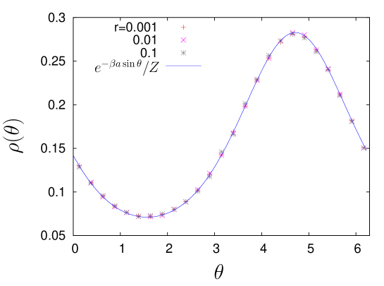
Figure 4: The points in the figure show the equilibrium density $\rho(\theta)$, obtained from numerical simulations of the dynamics (69) with $H=a\sin\theta$, and with $G=0$, $a=0.87s^{-1}$, $\beta=0.8s$, and for three values of $r=0.001,0.01$, and $0.1$. It can be seen that the results do not depend on the value of $r$. In the figure, the results of numerical simulations have also been compared with the analytical result given in (72) with $H=a\sin\theta$, and is represented in the figure by the continuous line.

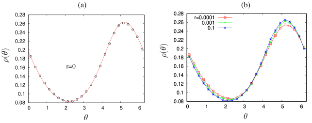
Figure 5: (a) The points represent the stationary density $\rho(\theta)$, obtained from numerical simulation of the dynamics (69) with $H=a\sin\theta$, and with $G=0.85s^{-1}$, $a=0.87s^{-1}$, $\beta=0.8s$, but without the Poisson noise ($r=0$). As expected, the points may be seen to lie on the continuous line representing the exact result in (LABEL:rhonP). (b) Here, we show the stationary density $\rho(\theta)$, obtained from numerical simulations of the dynamics (69) with $G=0.85s^{-1}$, $a=0.87s^{-1}$, $\beta=0.8s$, and for $r=0.0001,0.001$, and $0.1$. It is easily seen that $\rho(\theta)$ depends on the value of $r$, thereby hinting at the important role played by the Poisson noise.

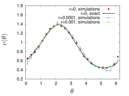
Figure 6: (a) The figure shows the local symmetric velocity $v(\theta)$ for the dynamics (69) with $H=a\sin\theta$, and with $G=0.85s^{-1}$, $a=0.87s^{-1}$, $\beta=0.8s$, and for $r=0$ (no Poisson noise), $0.0001$, and $0.001$. The points are obtained from numerical simulations of the dynamics and use of the formula (LABEL:vtheta). The exact result for the case $r=0$ is given by (71). It is easily seen that $v(\theta)$ depends on the value of $r$, i.e., on the details of the Poisson noise in the dynamics.

Next, we investigate numerically the case where the external force takes the value of the experiments Gom1 ($G=0.85s^{-1}$) for three different values of $r$ (which characterizes the role of the Poisson noise), namely, $r=0.0001,0.001$, and $0.1$. The corresponding forms of the stationary state distribution are shown in Fig. 5(b). From the figure, it is evident that in the presence of the external force, the form of the non-equilibrium stationary state depends on $r$, thereby underlying the importance of the Poisson noise. This is to be contrasted with the result for the case depicted in Fig. 4, i.e., with $G=0$, when the form of the equilibrium stationary state is independent of $r$. Corresponding to the non-equilibrium stationary state for $G\neq 0$, the local symmetric velocity (57,59,60) is given by

$$v(\theta) = -a\cos(\theta)+G-\frac{1}{\beta}\partial_{\theta}\left(\ln\rho(\theta)\right)$$

$$+\frac{r\exp(\frac{a\beta}{2}\sin(\theta))}{2}\left(\int_{0}^{2\pi}d\theta^{\prime}\exp\left(-\frac{\beta a}{2}\sin(\theta^{\prime})\right)\theta^{\prime}\right)$$

$$-\frac{r\rho^{-1}(\theta)\exp(-\frac{a\beta}{2}\sin(\theta))}{2}\left(\int_{0}^{2\pi}d\theta^{\prime}\rho(\theta^{\prime})\exp\left(\frac{\beta a}{2}\sin(\theta^{\prime})\right)\theta^{\prime}\right).$$

In Fig. 6, we show the local symmetric velocity $v(\theta)$ for the dynamics (69) with $G=0.85s^{-1}$, $a=0.87s^{-1}$, $\beta=0.8s$, and for $r=0$ (no Poisson noise), $0.0001$, and $0.001$. It is clear from the figure that the quantity $v(\theta)$ depends on the details of the Poisson noise in the dynamics.

In Section 5.3.1, we will use the dynamics (69) as a model system to verify the GFDT by extensive numerical simulations.

5 Perturbation of a Markov process: the Fluctuation-Dissipation Theorem

Suppose that our dynamics evolves for $t\leq 0$ with a given Markovian dynamics of generator $L_{t}$ and then suddenly, at time $t=0$, we perturb the dynamics such that the new Markov generator $L_{t}^{\prime}$ becomes

$$L_{t}^{\prime}=L_{t}+k_{t}N_{t},$$ (74)

with $k_{t}$ a real function, sometimes called the response field, and $N_{t}$ an operator. We will assume that the perturbed process still has the property to have honest transition probability (i.e., $N_{t}[1]=0).$ The FDT concerns the relation between correlation functions, (34), in the unperturbed state and response functions in the case of a small perturbation (i.e., $k_{t}$ infinitesimal).

5.1 Response function

The linear response theory allows to express the variation of the average of an observable under the perturbation as

$$\left.\frac{\delta\left\langle A_{t}(x_{t})\right\rangle^{\prime}}{\delta k_{s}}\right|_{k=0}=\left\langle\left(\rho_{s}^{-1}N^{\dagger}[\rho_{s}]\right)(x_{s})A_{t}(x_{t})\right\rangle,$$ (75)

where $\left\langle{}\right\rangle^{\prime}$ denotes expectation for the process with the generator $L_{t}^{\prime}.$ The proof of this relation is given in Appendix (C) for the convenience of the reader. Note however that this result is known for a long time in the physics literature Agarw ; Han ; Kubo0 ; Risk and now has a mathematically rigorous formulation (Definition $2.5$ in Dem1 ). This relation, besides being the basis for the FDT, allows to prove the Green-Kubo relation Kubo2 in the case of homogeneous perturbation ($k_{t}=k$) of a stationary dynamics. Note that other higher order relations may be derived in the context of the non-linear response theory Lip2 .

5.2 Hamiltonian perturbation class or generalized Doob $h$-transform

We will see that the form of the perturbation is the central point of the FDT, and it does not make sense to talk of FDT without giving its form. We want to begin by studying a class of (non-infinitesimal) perturbation of the Markov process such that the transformation of the generator can be expressed in terms of a family of non-homogeneous positive function $h_{t}$, as

$$L_{t}^{{}^{\prime}}=h_{t}^{-1}\circ L_{t}\circ h_{t}-h_{t}^{-1}L_{t}\left[h_{t}\right]\equiv L_{t}^{h}.$$ (76)

In the case where $\frac{d_{+}h_{t}}{dt}=\partial_{t}h_{t}+L_{t}\left[h_{t}\right]=0$ ($h_{t}(x)$ is the so-called space time harmonic function), such a transformation is classical in the probability literature and is called the Doob $h$-transform (or gauge transformation in physics literature). This was first introduced by Doob (Doo1 ; see also chapter 11 of Chu1 ), and plays an important role in the potential theory. We remark that if $h_{t}(x)$ is space-time harmonic, then $h_{t}(x_{t})$ is a martingale, i.e.,

$$h_{t}(x)=\mathbf{E}_{t,x}\left(h_{T}(x_{T})\right)~{}~{}~{}~{}~{}~{}~{}~{}~{}\forall~{}~{}T\geq t.$$ (77)

By introducing the symmetric bilinear operator $\Gamma$ (the so-called ”carre du champs” Rev1 , which can be roughly translated into English as “square of the field”, such that $\Gamma_{t}(f,g)=L_{t}\left[fg\right]-fL_{t}\left[g\right]-L_{t}\left[f\right]g$, the perturbed generator can be expressed in the form $L_{t}^{h}=L_{t}+h_{t}^{-1}\Gamma(h_{t},)$. A remarkable property of this type of perturbation appears if we restrict to a subclass of unperturbed processes which are in so-called local detailed balance (14) with the Gibbs density $\pi_{t}=\exp(-\beta H_{t})$. We then have the relation

$$h_{t}^{2}\pi_{t}\circ L_{t}^{h}\circ\left(h_{t}^{2}\pi_{t}\right)^{-1} =h_{t}\pi_{t}\circ L_{t}\circ\left(\pi_{t}\right)^{-1}h_{t}^{-1}-h_{t}^{-1}L_{t}(h_{t})$$ (78)

$$=h_{t}\circ L_{t}^{\dagger}\circ h_{t}^{-1}-h_{t}^{-1}L_{t}(h_{t})=\left(L_{t}^{h}\right)^{\dagger},$$

which implies that, for the perturbed process, the density, given by

$$\pi_{t}^{h}=\pi_{t}h_{t}^{2}=\exp(-\beta H_{t}+2\ln h_{t}),$$ (79)

is also in local detailed balance. This property of conservation of instantaneous infinitesimal detailed balance under the perturbation of the Hamiltonian $H\rightarrow H-\frac{2}{\beta}\ln h_{t}$  is the first justification for the name “Hamiltonian perturbation” that we chose for this type of perturbation. However, we stress that this perturbation, although called here “Hamiltonian perturbation”, is applicable to general Markov processes which do not have an underlying Hamiltonian which generates the dynamics. Moreover, for a general diffusion process, we can easily calculate (see Appendix (D)) the operator ”carre du champs”

$$\Gamma_{t}(f,g)=d_{t}^{ij}\left(\nabla_{i}f\right)\left(\nabla_{j}g\right).$$ (80)

Then the perturbed generator (76) is

$$L_{t}^{h}=L_{t}+d_{t}^{ij}\nabla_{j}\left(\ln\left|h_{t}\right|\right)\nabla_{i},$$ (81)

so that there is just a change of the drift term, $u_{t}^{i}\rightarrow u_{t}^{i}+d_{t}^{ij}\nabla_{j}(\ln h_{t}).$ In the subcase of an overdamped Langevin process (44), the perturbed process (76) becomes

$$\dot{x}^{i}\ =\ -\Gamma_{t}^{ij}(x)\partial_{j}\left(H_{t}(x)-\frac{2}{\beta}\ln h_{t}\right)+G_{t}^{i}(x)+\frac{\partial_{y^{j}}\left.D_{t}^{ij}(x,y)\right|_{x=y}}{{}^{2}}+\,\eta_{t}^{i}(x)\,.$$ (82)

So we see that the perturbation in (76) is once again equivalent to change of the Hamiltonian, $H\rightarrow H-\frac{2}{\beta}\ln h_{t}$. Now we want to show that the type of perturbation in (76) includes the perturbation usually considered in the articles on FDT that exist in the literature.

• For pure jump process, it is usual to ask precisely the property of conservation of this local detailed balance for the Gibbs density $\pi_{t}=\exp(-\beta H_{t})$ under the perturbation of the Hamiltonian $H\rightarrow H-k_{t}O_{t}$. We see from (79) that this perturbation of the Hamiltonian is of the type in (76), with the choice

  $$h_{t}=\exp\left(\frac{\beta}{2}k_{t}O_{t}\right).$$ (83)

  This implies the following transformation for the transition rates.

  $$W_{t}^{h}(x,y)=\exp\left(-\frac{\beta}{2}k_{t}O_{t}(x)\right)W_{t}(x,y)\exp\left(\frac{\beta}{2}k_{t}O_{t}(y)\right).$$ (84)

  This is the perturbation considered recently in Bae1 and earlier in Die1 for finding the GFDT in this pure jump process set-up.

• For overdamped Langevin process, it is usual Han ; Kubo0 ; MPRV ; Risk to do a perturbation of the Hamiltonian, $H\rightarrow H-k_{t}O_{t}$, in (44). With (82), we see that it is of the type in (76) with once again (83) valid.

• Finally, we remark that for a jump diffusion process of type (52), this perturbation consists of a change of the drift according to $u_{t}^{i}\rightarrow u_{t}^{i}+d_{t}^{ij}\nabla_{j}(\ln h_{t})$ and simultaneously, a perturbation of the jump process by replacing the transition rates (56) by

  $$W_{t}^{h}(x,y)=h_{t}^{-1}(x)W_{t}(x,y)h_{t}(y).$$

  For the jump Langevin process (63), with the transition rates (64) for the Poisson noise, we can prove easily that the choice (83) in (76) is equivalent to the perturbation of the Hamiltonian according to $H\rightarrow H-k_{t}O_{t}.$

5.3 Fluctuation-Dissipation Theorem for Hamiltonian perturbation

In the case of an infinitesimal $h_{t}$ function,

$$h_{t}(x)=1+k_{t}B_{t}(x)+O(k^{2}),$$ (85)

we find that the Hamiltonian perturbation (76) has the infinitesimal form (74) with

$$N_{t}=L_{t}\circ B_{t}-B_{t}\circ L_{t}-L_{t}[B_{t}]\mathcal{I}.$$ (86)

The central point of the proof that follows is the fact that the observable $\rho^{-1}N_{t}^{\dagger}[\rho]$, which appears on the right hand side of (75), can be expressed in terms of the stochastic derivative (associated with the unperturbed process) of the observable $B_{t}$.

$$\rho_{t}^{-1}N_{t}^{\dagger}[\rho_{t}] =B_{t}\rho_{t}^{-1}L^{\dagger}[\rho_{t}]-\rho_{t}^{-1}\circ L^{\dagger}\circ\rho_{t}[B_{t}]-L_{t}[B_{t}]$$ (87)

$$=-(L_{t}+L_{t}^{\ast})[B_{t}]=\left(\frac{d_{-}}{dt}-\frac{d_{+}}{dt}\right)[B_{t}],$$

where the third equality comes from (30). We can rewrite this observable by adding a term proportional to $\left(2\frac{d}{dt}-\frac{d_{-}}{dt}-\frac{d_{+}}{dt}\right)B$ (which is exactly equal to zero), and then, for all $\alpha$, we get

$$\rho_{t}^{-1}N_{t}^{\dagger}[\rho_{t}]=\left(1-\alpha\right)\frac{d_{-}}{dt}B_{t}-(1+\alpha)\frac{d_{+}}{dt}B_{t}+2\alpha\frac{d}{dt}B_{t}.$$ (88)

Now, by using the response relation, (75) and the time derivative of a correlation function, (35), we find the family, indexed by $\alpha$ , of equivalent GFDT.

$$\left.\frac{\delta\left\langle A_{t}(x_{t})\right\rangle^{\prime}}{\delta k_{s}}\right|_{k=0}$$

$$=\left(1-\alpha\right)\partial_{s}\left\langle B_{s}(x_{s})A_{t}(x_{t})\right\rangle-(1+\alpha)\left\langle\frac{d_{+}B_{s}}{ds}(x_{s})A_{t}(x_{t})\right\rangle+2\alpha\left\langle\frac{dB_{s}}{ds}(x_{s})A_{t}(x_{t})\right\rangle.$$

Two particular cases of $\alpha$ exist in the literature:

• $\alpha=0$  : First GFDT

  $$\left.\frac{\delta\left\langle A_{t}(x_{t})\right\rangle^{\prime}}{\delta k_{s}}\right|_{k=0} = \partial_{s}\left\langle B_{s}(x_{s})A_{t}(x_{t})\right\rangle-\left\langle\frac{d_{+}B_{s}}{ds}(x_{s})A_{t}(x_{t})\right\rangle$$

  $$= \partial_{s}\left\langle B_{s}(x_{s})A_{t}(x_{t})\right\rangle-\left\langle\left(\partial_{s}B_{s}\right)(x_{s})A_{t}(x_{t})\right\rangle-\left\langle\left(LB\right)_{s}(x_{s})A_{t}(x_{t})\right\rangle.$$

In the usual case of Hamiltonian perturbation of a jump process or an overdamped Langevin process, with (83), we find $B_{t}=\frac{\beta}{2}O_{t}$ and then

$$\frac{2}{\beta}\left.\frac{\delta\left\langle A_{t}(x_{t})\right\rangle^{\prime}}{\delta k_{s}}\right|_{k=0} =\partial_{s}\left\langle O_{s}(x_{s})A_{t}(x_{t})\right\rangle-\left\langle\frac{d_{+}O_{s}}{ds}(x_{s})A_{t}(x_{t})\right\rangle$$

$$=\partial_{s}\left\langle O_{s}(x_{s})A_{t}(x_{t})\right\rangle-\left\langle\left(\partial_{s}O_{s}\right)(x_{s})A_{t}(x_{t})\right\rangle-\left\langle\left(LO\right)_{s}(x_{s})A_{t}(x_{t})\right\rangle,$$

which was first written down in Cug1 for diffusion process with additive noise and recently in Bae1 ; Bae2 ; Lip1 ; Liu2 ; Sei2 for jump process and overdamped Langevin process. The equilibrium limit (1) is a bit obscure; it may be seen by noting that one has $\left\langle\left(LO\right)(x_{s})A(x_{t})\right\rangle=\left\langle A(x_{s})\left(LO\right)(x_{t})\right\rangle=\partial_{t}\left\langle A(x_{s})O(x_{t})\right\rangle$. However, there exists physical interpretation of the new term $\left\langle\left(LB\right)_{s}(x_{s})A_{t}(x_{t})\right\rangle$ as the “frenetic term” Bae1 ; Bae2 .

• $\alpha=-1$ : Second GFDT

$$\frac{1}{2}\left.\frac{\delta\left\langle A_{t}(x_{t})\right\rangle^{\prime}}{\delta k_{s}}\right|_{k=0}=\partial_{s}\left\langle B_{s}(x_{s})A_{t}(x_{t})\right\rangle-\left\langle\frac{dB_{s}}{ds}(x_{s})A_{t}(x_{t})\right\rangle,$$ (94)

which has the advantage that the effect of the nonequilibrium character of the unperturbed state is just in the second term on the right hand side. For a diffusion process, this GFDT can be written Fal2 ; Che3 ; Che4 , with (49), as

$$\frac{1}{2}\left.\frac{\delta\left\langle A_{t}(x_{t})\right\rangle^{\prime}}{\delta k_{s}}\right|_{k=0}=\partial_{s}\left\langle B_{s}(x_{s})A_{t}(x_{t})\right\rangle-\left\langle\left(\partial_{s}B_{s}\right)(x_{s})A_{t}(x_{t})\right\rangle-\left\langle\left(V_{s}^{c}.\nabla B_{s}\right)(x_{s})A_{t}(x_{t})\right\rangle.$$ (95)

This GFDT was experimentally checked in Gom1 . In the usual case of Hamiltonian perturbation of a pure jump process or a overdamped Langevin process, with (83), we find

$$\frac{1}{\beta}\left.\frac{\delta\left\langle A_{t}(x_{t})\right\rangle^{\prime}}{\delta k_{s}}\right|_{k=0}=\partial_{s}\left\langle O_{s}(x_{s})A_{t}(x_{t})\right\rangle-\left\langle\frac{dO_{s}}{ds}(x_{s})A_{t}(x_{t})\right\rangle.$$ (96)

5.3.1 Example of jump Langevin equation (4.3.2).

Here, we want to numerically verify the GFDT (94) for a Markov process which mixes jump and diffusion. We consider the stochastic dynamics (69) with $H=a\sin\theta$ and the same values for the parameters as those considered in (4.3.2); $a=0.87s^{-1}$, $G=0.85s^{-1}$, $\beta=0.8s$, and $r=0.001$. The process is supposed to be at time $t\leq 0$ in the stationary state with $\rho(\theta)$ given in Fig. 5(b). Then, suddenly, at $t=0$, we consider a static perturbation of the Hamiltonian according to

$$H^{\prime}=H-k\sin\theta=\left(a-k\right)\sin\theta.$$ (97)

We saw in the last section that this perturbation is of the form (76 ), with

$$h(\theta)=\exp\left(\frac{\beta}{2}k\sin\theta\right).$$ (98)

We checked numerically the time integrated version of the FDT (96 ) around steady state for $A=B=\sin\theta$.

$$\frac{1}{\beta}\frac{\partial}{\partial k}\left.\left\langle\sin\theta_{t}\right\rangle^{\prime}\right|_{k=0}=\left\langle\sin^{2}\theta_{t}\right\rangle-\left\langle\sin\theta_{0}\sin\theta_{t}\right\rangle-\int_{0}^{t}ds\left\langle C(\theta_{s})\sin\theta_{t}\right\rangle.$$ (99)

The form of the observable $C(\theta)\equiv\frac{d\sin\theta_{t}}{dt}(\theta)$ is found with the help of (61) as

$$C(\theta) =\left(-a\cos(\theta)+G-\frac{1}{\beta}\left(\partial_{\theta}\ln\rho\right)\right)\cos\theta$$ (100)

$$+\frac{\left(\int d\theta^{\prime}W(\theta,\theta^{\prime})\left(\sin\left(\theta^{\prime}\right)-\sin(\theta)\right)\right)}{2}$$

$$-\frac{\rho^{-1}(\theta)\left(\int d\theta^{\prime}\left(\sin\left(\theta^{\prime}\right)-\sin(\theta)\right)\rho(\theta^{\prime})W(\theta^{\prime},\theta)\right)}{2},$$

with $W(\theta,\theta^{\prime})$ given by (64)

$$W(\theta,\theta^{\prime})=r\exp\left(-\frac{\beta a}{2}\left(\sin(\theta^{\prime})-\sin(\theta)\right)\right).$$ (101)

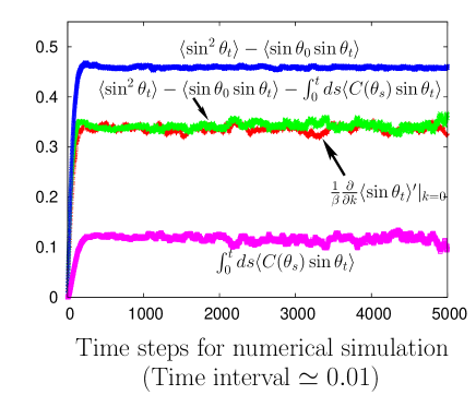
Figure 7: Based on our results from numerical simulations of the dynamics (69) with $H=a\sin\theta$, the figure shows the different terms in the integrated version of the GFDT (99). Here, $a=0.87s^{-1}$, $G=0.85s^{-1}$, $\beta=0.8s$, and the parameter $r=0.001$. One observes a satisfactory agreement between the left hand side $\frac{1}{\beta}\frac{\partial}{\partial k}\langle\sin\theta_{t}\rangle^{\prime}|_{k=0}$ and the right side $\left\langle\sin^{2}\theta_{t}\right\rangle-\left\langle\sin\theta_{0}\sin\theta_{t}\right\rangle-\int_{0}^{t}ds\left\langle C(\theta_{s})\sin\theta_{t}\right\rangle$ of the GFDT (99), which therefore verifies the theorem.

Figure 7 shows results from our numerical simulations for the various terms in the integrated version of the GFDT (99). In the figure, one can observe a satisfactory agreement between the left hand side and the right side of (99), thereby verifying the GFDT.

5.4 Fluctuation-Dissipation Theorem for a more general class of perturbation

We will now consider a larger class of perturbation than (76) such the perturbation can be expressed in terms of two family of non-homogeneous functions $h_{t}$ and $h_{t}^{\prime}$, as

$$L_{t}^{\prime}=h_{t}^{-1}\circ L_{t}\circ h_{t}^{\prime}-h_{t}^{-1}\circ L_{t}[h_{t}^{\prime}],$$ (102)

which specializes to the Hamiltonian perturbation (76) when $h=h^{\prime}$. We will see in the following subsections two physical perturbations, the time change and the thermal perturbation, which belong to this class. In the case of infinitesimal perturbation,

$$h_{t}=1+k_{t}B_{t}+O(h^{2})\text{ \ \ and \ }h_{t}^{\prime}=1+k_{t}B_{t}^{\prime}+O(h^{2}),\text{ \ }$$ (103)

we find that this perturbation has the form (74) with

$$N_{t}=-B_{t}\circ L_{t}+L_{t}\circ B_{t}^{\prime}-L_{t}[B_{t}^{\prime}].$$ (104)

For a pure discontinuous process, the perturbation (102) implies for the transition rates, $W_{t}^{\prime}=h_{t}^{-1}\circ W_{t}\circ h_{t}^{\prime}$, and was considered in Die1 and more recently in Mae3 by taking $h_{t}(x)=\exp(\mu\beta k_{t}O(x))$ and $h_{t}^{\prime}(x)=\exp(\gamma\beta k_{t}O(x))$, where $O(x)$ is an observable, and $\mu$ and $\gamma$ two real numbers. As in ( 87), we show that the observable $\rho_{t}^{-1}N_{t}^{\dagger}[\rho_{t}]$, which appears on the right hand side of (75), can be expressed in terms of the stochastic derivative of $B_{t}$ and $B_{t}^{\prime}$ as

$$\rho^{-1}N^{+}[\rho] =-\rho^{-1}\circ L^{\dagger}\circ\rho[B]+B^{\prime}\rho^{-1}L^{\dagger}[\rho]-L[B^{\prime}]$$

$$=-L^{\ast}\left[B\right]-B\rho^{-1}L^{\dagger}[\rho]+B^{\prime}\rho^{-1}L^{\dagger}[\rho]-L[B^{\prime}]$$

$$=\left\{\begin{array}[]{c}\left(\partial_{t}+\rho^{-1}L^{\dagger}[\rho]\right)(-B+B^{\prime})+\frac{d_{-}B}{dt}-\frac{d_{+}B^{\prime}}{dt}\\ \text{or},~{}~{}~{}\left(\partial_{t}+\rho^{-1}L^{\dagger}[\rho]\right)(-B+B^{\prime})+\frac{d_{-}\left(B^{\prime}+B\right)}{dt}-2\frac{dB^{\prime}}{dt}.\end{array}\right.$$

We obtain then the generalization of the first GFDT (LABEL:TFD1)

$$\left.\frac{\delta\left\langle A_{t}(x_{t})\right\rangle^{\prime}}{\delta k_{s}}\right|_{k=0}$$

$$=\partial_{s}\left\langle B_{s}(x_{s})A_{t}(x_{t})\right\rangle-\left\langle\frac{d_{+}B_{s}^{\prime}}{ds}(x_{s})A_{t}(x_{t})\right\rangle$$

$$+\left\langle\left(\left(\partial_{s}+\rho_{s}^{-1}L_{s}^{\dagger}[\rho_{s}]\right)(B_{s}^{\prime}-B_{s})\right)(x_{s})A_{t}(x_{t})\right\rangle,$$ (106)

and the second GFDT (94)

$$\left.\frac{\delta\left\langle A_{t}(x_{t})\right\rangle^{\prime}}{\delta k_{s}}\right|_{k=0}$$

$$=\partial_{s}\left\langle\left(B_{s}^{\prime}+B_{s}\right)(x_{s})A_{t}(x_{t})\right\rangle-2\left\langle\frac{dB_{s}^{\prime}}{ds}(x_{s})A_{t}(x_{t})\right\rangle$$

$$+\left\langle\left(\left(\partial_{s}+\rho_{s}^{-1}L_{s}^{\dagger}[\rho_{s}]\right)(B_{s}^{\prime}-B_{s})\right)(x_{s})A_{t}(x_{t})\right\rangle.$$ (107)

We see that in the Hamiltonian perturbation class (i.e., $B=B^{\prime}$), we recover the GFDT (LABEL:TFD1,94).

5.4.1 Around Steady State

We will now restrict to the case where the observable does not have explicit time dependence (i.e., $A_{t}=A$, $B_{t}=B,B_{t}^{\prime}=B^{\prime})$, and the unperturbed state is a steady state. Then the first GFDT ( 106) becomes

$$\left.\frac{\delta\left\langle A(x_{t})\right\rangle^{\prime}}{\delta k_{s}}\right|_{k=0}=\partial_{s}\left\langle B(x_{s})A(x_{t})\right\rangle-\left\langle\frac{d_{+}B^{\prime}}{ds}(x_{s})A(x_{t})\right\rangle,$$ (108)

and the second (107) becomes

$$\left.\frac{\delta\left\langle A(x_{t})\right\rangle^{\prime}}{\delta k_{s}}\right|_{k=0}=\partial_{s}\left\langle\left(B+B^{\prime}\right)(x_{s})A(x_{t})\right\rangle-2\left\langle\frac{dB^{\prime}}{ds}(x_{s})A(x_{t})\right\rangle.$$ (109)

In the case where the steady state is of equilibrium-type (i.e. $\frac{d}{ds}=\partial_{s}$), this last relation (109) simplifies to the form

$$\left.\frac{\delta\left\langle A(x_{t})\right\rangle^{\prime}}{\delta k_{s}}\right|_{k=0}=\partial_{s}\left\langle\left(B+B^{\prime}\right)(x_{s})A(x_{t})\right\rangle.$$ (110)

5.4.2 Time change for a homogeneous Markov process Dem1

An example of perturbation which belongs to the generalized class (102) but not to the Hamiltonian perturbation class (76) is when we consider the change of clock as follows.

$$t^{f}(s)\equiv\int_{0}^{s}du\exp\left(f_{u}\left(x_{u}\right)\right),$$ (111)

where $f_{u}$ is an observable. It is proved in Dem1 (proposition 3.1) that the process $x_{s}^{\prime}=x_{t^{f}(s)}$ is still Markov with a generator $L_{t}^{{}^{\prime}}=\exp(-f_{t})L$. In the case of infinitesimal perturbation $f_{u}(x)=k_{u}B(x)$, $L_{t}^{{}^{\prime}}=L-k_{t}BL$, which is of the form (104) with $B^{\prime}=0$ so that the FDT ( 106, 107) takes the form

$$\left.\frac{\delta\left\langle A(x_{t})\right\rangle^{\prime}}{\delta k_{s}}\right|_{k=0}=\partial_{s}\left\langle B(x_{s})A(x_{t})\right\rangle-\left\langle\left(\rho_{s}^{-1}L^{\dagger}[\rho_{s}]B\right)(x_{s})A(x_{t})\right\rangle.$$ (112)

In the case of an unperturbed system in the steady state, (108,109) become the usual FDT.

$$\left.\frac{\delta\left\langle A(x_{t})\right\rangle^{\prime}}{\delta k_{s}}\right|_{k=0}=\partial_{s}\left\langle B(x_{s})A(x_{t})\right\rangle,$$ (113)

which is a result of Dem1 . We want to emphasize that, for this type of perturbation, we obtain the usual FDT (without correction) for an unperturbed state which is a general nonequilibrium steady state.

5.4.3 Thermal Perturbation Pulse : Change of temperature for equilibrium overdamped Langevin process

A famous example in physics for a perturbation which is not of Hamiltonian type is thermal perturbation. Let us consider a system whose dynamics is governed by (44), with $G=0$ and homogeneous Hamiltonian, and the perturbed system which results from the change of the bath temperature $\,\beta_{t}^{-1}=(1+k_{t})\beta^{-1}.$ We can easily prove that

$$N=\frac{1}{\beta}\nabla_{i}\circ\Gamma^{ij}\circ\nabla_{j},$$ (114)

which is of the form of the general infinitesimal perturbation (104) with $B^{\prime}=\frac{\beta H}{2}$  and $B=\frac{\beta H}{2}-1.$ This can be easily seen by using the formula (80) for the ”carre du champs”:

$$L\circ B^{\prime}-L[B^{\prime}]=B^{\prime}L+\Gamma(B^{\prime},.)=B^{\prime}L+\frac{2\Gamma^{ij}}{\beta}\left(\nabla_{i}B^{\prime}\right)\nabla_{j}=\frac{\beta H}{2}L-L+N.$$ (115)

The formula (110) then takes the form $\left.\frac{\delta\left\langle A_{t}(x_{t})\right\rangle^{\prime}}{\delta k_{s}}\right|_{k=0}=\partial_{s}\left\langle\left(\beta H-1\right)(x_{s})A_{t}(x_{t})\right\rangle$, which implies the equilibrium form

$$\frac{1}{\beta}\left.\frac{\delta\left\langle A_{t}(x_{t})\right\rangle^{\prime}}{\delta k_{s}}\right|_{h=0}=\partial_{s}\left\langle H(x_{s})A_{t}(x_{t})\right\rangle.$$ (116)

In particular, we obtain the usual FDT for the energy Risk .

$$\frac{1}{\beta}\left.\frac{\delta\left\langle H(x_{t})\right\rangle^{\prime}}{\delta k_{s}}\right|_{k=0}=\partial_{s}\left\langle H(x_{s})H(x_{t})\right\rangle.$$ (117)

6 Two families of non-perturbative extensions of the Fluctuation-Dissipation Theorem

It is well understood since the discovery of the FR that they may be viewed as extensions to the non-perturbative regime of the Green-Kubo and Onsager relations which are usually valid within the linear response description in the vicinity of equilibrium Gall2 ; LebowSp . A detailed proof was given in Che1 that the Jarzynski equality gives the usual FDT when expanded to second order in the response field. In Fal2 , it was proved that this correspondence is still true around an unperturbed state which is stationary but out of equilibrium) . This is proved by doing a Taylor expansion of a special Crooks theorem to first order in the response field. Finally, in Che4 , general FR were exhibited which are global versions of the GFDT for nonequilibrium diffusion, or, of the FDT for energy resulting from a thermal perturbation. We introduce in Section (6.1) a first family of exponential martingales which is a natural object associated with the perturbation (76), and show in Section (6.1.3) that these are global version of general GFDT (LABEL:TFD1,94). Section (6.2) presents the martingale property of functionals which appear in the fluctuation relations and it shows their relation to the exponential martingales introduced in Section (6.1). Along the way, we prove the FR along the lines of the proof given below for the exponential martingale by a comparison to the backward process generated by the Doob $h$-transform of the adjoint generator $L^{\dagger}$.

6.1 New family of exponential martingales naturally related to GFDT

6.1.1 Introduction

We come back to the perturbation (76) of the generator,

$$L_{t}^{h}\equiv h_{t}^{-1}\circ L_{t}\circ h_{t}-h_{t}^{-1}L_{t}\left[h_{t}\right],$$ (118)

but this time we will not restrict to the regime where $h_{t}$ is infinitesimal. We prove in Appendix (E) that the Markov process associated with the generators $L_{t}^{h}$ and $L_{t}$ are related through the functional $\exp(-\mathbf{Z}_{s}^{h,t})$ by

$$P_{s}^{h,t}(x,y)=\mathbf{E}_{s,x}\left[\delta(x_{t}-y)\exp(-\mathbf{Z}_{s}^{h,t})\right],$$ (119)

where

$$\exp(-\mathbf{Z}_{s}^{h,t}\left[x\right])=h_{s}^{-1}(x_{s})\exp\left(-\int_{s}^{t}du\left(h_{u}^{-1}L_{u}\left[h_{u}\right]+h_{u}^{-1}\partial_{u}h_{u}\right)(x_{u})\right)h_{t}(x_{t}).$$ (120)

The functional $\exp(-\mathbf{Z}_{s}^{h,t})$ is multiplicative:

$$\exp(-\mathbf{Z}_{s}^{h,t})=\exp(-\mathbf{Z}_{s}^{h,u})\,\exp(-\mathbf{Z}_{u}^{h,t})$$ (121)

for $s\leq u\leq t$. The perturbation (118) is a particular case of the transformation of a Markov process by multiplicative functionals Blu1 ; Ito . It is a generalization of the Doob $h$-transform, which is

$$P_{s}^{h,t}(x,y)=h_{s}^{-1}(x)P_{s}^{t}(x,y)h_{t}(y),$$ (122)

in the case where $h_{t}(x)$ is the space-time harmonic function, i.e. $\frac{d_{+}h}{dt}=0$.

Thanks to the Markovian structure of the trajectory measure, the relation (119) for the transition probability is equivalent (as proved in Appendix F) to the relation between the expectations of functionals of the paths from time $s$ to time $t$ for the perturbed and the unperturbed processes,

$$\mathbf{E}_{s,x}^{h}\left[F_{\left[s,t\right]}\right]=\mathbf{E}_{s,x}\left[F_{\left[s,t\right]}\exp(-\mathbf{Z}_{s}^{h,t}[x])\right],$$ (123)

where $\mathbf{E}_{s,x}^{h}\left[{~{}~{}}\right]$ denotes expectation for the process with generators $L_{t}^{h}.$

Finally, we can also formulate (123) by requiring that the perturbed process with generators $L_{t}^{h}$ and trajectory measure $M_{\mu_{0,}\left[s,t\right]}^{h}$, can be obtained from the unperturbed process with trajectory measure $M_{\mu_{0,}\left[s,t\right]}$ by using the likelihood ratio process (the Radon-Nikodym density):

$$M_{\mu_{0,}\left[s,t\right]}^{h}[x]=M_{\mu_{0,}\left[s,t\right]}[x]{\frac{\rho^{h}_{s}}{\rho_{s}}(x_{s})}\exp(-\mathbf{Z}_{s}^{h,t}[x]),$$ (124)

with $\rho_{s}(x)=\int dy\rho_{0}(y)P_{0}^{s}(y,x)$ the instantaneous density of the original process and $\rho^{h}_{s}(x)=\int dy\rho_{0}(y)P_{0}^{h,s}(y,x)$ the instantaneous density of the $h$-transformed process.

We could not find the general result (120,123,124) in the mathematics literature, but many very closely related results do exist. The subcase of (123,124) where $h_{t}$ is time-homogeneous (i.e., $\partial_{t}h_{t}=0)$) was treated long time ago by Kunita in Kun1 and was revisited recently in the articles Pal1 and Dia1 . In our context of the FDT, the extension to $\partial_{t}h_{t}\neq 0$ is essential. But more than generalizing to $\partial_{t}h_{t}\neq 0,$ the main interest in the Appendices (E,F) is to prove (123) from theoretical physics perspective. We recall also that for a diffusion process, the perturbed generator (118) is obtained by adding the term $d_{t}\nabla\left(\ln h_{t}(x)\right)$ to the drift (see (81)). Then, the proofs in Appendices (E,F) are also a theoretical physicist’s proofs of the Girsanov theorem for a diffusion process Rev1 (for this type of change of drift).

6.1.2 Martingale properties of the functional $\exp(-\mathbf{Z}_{s}^{t}$)

The multiplicative functional $\exp(-\mathbf{Z}_{s}^{h,t}\left[x\right])$ is an exponential martingale with respect to the natural $\sigma$-algebra filtration $\mathcal{F}_{t}=\sigma(x_{s},s\leq t)$ representing the increasing flow of information. This fact can be seen by first noting that (123) (with $F=1$) implies the normalization condition

$$\mathbf{E}_{s,x}\left[\exp\left(-\mathbf{Z}_{s}^{h,t}\left[x\right]\right)\right]=1,$$ (125)

which, thanks to the multiplicative structure of $\exp(-\mathbf{Z}_{s}^{h,t}\left[x\right])$, yields

$$\mathbf{E}\left[\exp(-\mathbf{Z}_{s}^{h,t}\left[x\right])|\mathcal{F}_{u}\right]=\exp(-\mathbf{Z}_{s}^{h,u}\left[x\right])\mathbf{E}_{x_{u},u}\left[\exp(-\mathbf{Z}_{u}^{h,t}\left[x\right])\right]=\exp(-\mathbf{Z}_{s}^{h,u}\left[x\right]),$$ (126)

for $s\leq u\leq t.$

6.1.3 Fluctuation-Dissipation Theorem as Taylor expansion of the exponential martingale identity (123)

In the infinitesimal case, $h_{t}(x)=1+k_{t}B_{t}(x)+O(k^{2})$, Taylor expansion of the subcase of (123) with one-point functional $F_{\left[s,t\right]}[x]=A_{t}(x_{t})$, namely,

$$\left\langle A_{t}(x_{t})\right\rangle^{h}=\left\langle\left(h_{s}\right)^{-1}(x_{s})\exp\left(\int_{s}^{t}du\left(-h_{u}^{-1}L_{u}\left[h_{u}\right]-h_{u}^{-1}\partial_{u}h_{u}\right)(x_{u})\right)h_{t}(x_{t})A_{t}(x_{t})\right\rangle,$$ (127)

gives, to the first order in $\left[k\right]$,

$$\left\langle A_{t}(x_{t})\right\rangle^{h}-\left\langle A_{t}(x_{t})\right\rangle-\left\langle\left(h_{s}\right)^{-1}(x_{s})A_{t}(x_{t})\right\rangle-\left\langle\left(h_{t}\right)(x_{t})A_{t}(x_{t})\right\rangle$$

$$+\int_{s}^{t}du\left\langle\frac{d_{+}h_{u}}{du}(x_{u})A_{t}(x_{t})\right\rangle+O(k^{2})=0.$$ (128)

To find the first GFDT (LABEL:TFD1) from (128), we use the direct differentiation formula $\frac{d_{+}h_{u}}{du}=\frac{d_{+}\left(k_{u}B_{u}\right)}{du}=\left(\partial_{u}k_{u}\right)B_{u}+k_{u}\frac{d_{+}\left(B_{u}\right)}{du}$ obtaining the relation

$$\left.\frac{\delta\left\langle A_{t}(x_{t})\right\rangle^{\prime}}{\delta k_{u}}\right|_{k=0}-\partial_{u}\left\langle B_{u}(x_{u})A_{t}(x_{t})\right\rangle+\left\langle\frac{d_{+}B_{u}}{du}(x_{u})A_{t}(x_{t})\right\rangle=0,$$ (129)

which is the GFDT (LABEL:TFD1) (note the equivalence of the two notations $\left\langle{\ }\right\rangle^{\prime}$ and $\left\langle{\ }\right\rangle^{h})$). To find the second GFDT (94) from (128), we use the formula $d_{+}=2d-d_{-}$, which gives

$$\left\langle A_{t}(x_{t})\right\rangle^{h}-\left\langle A_{t}(x_{t})\right\rangle-\left\langle\left(h_{s}\right)^{-1}(x_{s})A_{t}(x_{t})\right\rangle-\left\langle\left(h_{t}\right)(x_{t})A_{t}(x_{t})\right\rangle$$

$$+2\int_{s}^{t}du\left\langle\frac{dh_{u}}{du}(x_{u})A_{t}(x_{t})\right\rangle-\int_{s}^{t}du\left\langle\frac{d_{-}h_{u}}{du}(x_{u})A_{t}(x_{t})\right\rangle+O(k^{2})=0.\qquad$$ (130)

Then, by using (35) for the time derivative of a correlation function, we obtain

$$\left\langle A_{t}(x_{t})\right\rangle^{h}-\left\langle A_{t}(x_{t})\right\rangle-\left\langle\left(h_{s}\right)^{-1}(x_{s})A_{t}(x_{t})\right\rangle-\left\langle\left(h_{t}\right)(x_{t})A_{t}(x_{t})\right\rangle+$$

$$2\int_{s}^{t}du\left\langle\frac{dh_{u}}{du}(x_{u})A_{t}(x_{t})\right\rangle-\int_{s}^{t}du\partial_{u}\left\langle h_{u}(x_{u})A_{t}(x_{t})\right\rangle+O(k^{2})=0.\qquad$$ (131)

Next, we use the differentiation formula $\frac{dh_{u}}{du}=\frac{d\left(k_{u}B_{u}\right)}{du}=\left(\partial_{u}k_{u}\right)B_{u}+k_{u}\frac{d\left(B_{u}\right)}{du}$ to get

$$\left.\frac{\delta\left\langle A_{t}(x_{t})\right\rangle^{\prime}}{\delta k_{u}}\right|_{k=0}-2\partial_{u}\left\langle B_{u}(x_{u})A_{t}(x_{t})\right\rangle+2\left\langle\frac{dB_{u}}{du}(x_{u})A_{t}(x_{t})\right\rangle=0,$$ (132)

which is (94). This gives a second independent proof of (LABEL:TFD1, 94). It also shows that the above exponential martingales are natural global versions of the GFDT. We will discuss in the next section another well known global version, namely, the Fluctuation Relations (FR).

6.2 Family of exponential martingales related to GFDT through Fluctuation Relations

6.2.1 Introduction to Fluctuation Relations

Roughly speaking, FR may be obtained by comparing the expectation of functionals of trajectories of the system and of reversed trajectories of the so-called backward system (denoted by an index $r$) . More precisely, let us denote by $M^{r}_{\mu_{0}^{r},\left[0,T\right]}$ the trajectorial measure of the backward process which is initially distributed with the measure $\mu_{0}^{r}(dx)\equiv\rho_{0}^{r}(x)dx$. Next, we define the path-wise time inversion $R$ at fixed time $T$, which acts on the space of trajectories according to $R\left[x\right]_{t}=\left[x\right]_{T-t}$. This allows us to introduce the (push-forward) measure $R_{\ast}\left(M_{\mu_{0},\left[0,T\right]}\right)$, which is the measure of the trajectory but traversed in the backward sense. We then introduce the action functional $\mathbf{W_{0}^{T}}$ through the Radon Nykodym derivative of the image measure of the backward system $R_{\ast}\left(M^{r}_{\mu_{0}^{r},\left[0,T\right]}\right)$ with respect to the trajectorial measure $M_{\mu_{0},\left[0,T\right]}$ of the forward system (initially distributed with the measure $\mu_{0}(dx)\equiv\rho_{0}(x)dx$):

$$R_{\ast}\left(M^{r}_{\mu_{0}^{r},\left[0,T\right]}\right)\equiv\exp\left(-\mathbf{W}_{0}^{T}\right)M_{\mu_{0},\left[0,T\right]}.$$ (133)

Equivalently, we can write this relation in the form of the Crooks theorem Maes ; Crooks2 ; LebowSp ; Sch1 ; Che1 ; Liu1 ; Sei2 asserting that for all trajectory functionals $F_{\left[0,T\right]}$,

$$\left\langle F_{\left[0,T\right]}\circ R\right\rangle^{r}=\left\langle F_{\left[0,T\right]}\exp\left(-\mathbf{W}_{0}^{T}\right)\right\rangle.$$ (134)

Finally, by the substitution $F_{\left[0,T\right]}\left[x\right]\rightarrow F_{\left[0,T\right]}\left[x\right]\delta(x_{0}-y)]\delta(x_{T}-x),$ we find the equivalent relation,

$$\rho_{0}^{r}(x)\mathbf{E}_{0,x}^{r}\left[F_{\left[0,T\right]}\circ R\left[x\right]\delta(x_{T}-y)\right]$$ (135)

$$\hskip 42.67912pt=\rho_{0}(y)\mathbf{E}_{0,y}\left[F_{\left[0,T\right]}\left[x\right]\exp\left(-\mathbf{W}_{0}^{T}\left[x\right]\right)\delta(x_{T}-x)\right].$$ (136)

Due to the freedom in choosing the initial forward measure $\mu_{0}$ or the backward measure $\mu_{0}^{r}$, it is possible to identify the action functional with various thermodynamic quantities like the work performed on the system or the fluctuating entropy creation $\mathbf{\sigma}_{0}^{T}\left[x\right]$ with respect to the inversion $r$ . This latter quantity is obtained when $\mu_{0}^{r}(dx)=\rho_{0}^{r}(x)dx=\rho_{T}(x)dx\equiv\int dy\rho_{0}(y)P_{0}^{T}(y,x)dx$. We can also obtain the functional entropy production in the environment, $\mathbf{J}_{0}^{T}$, by choosing $\mu_{0}(dx)=\mu_{0}^{r}(dx)=dx$, because then the difference from the entropy creation is the boundary term $\ln\left(\rho_{0}(x_{0})\right)-\ln\left(\rho_{t}(x_{t})\right)$, which gives the change in the instantaneous entropy of the process.

Let us observe the similarity between (123,124 ) and (136,133); $\exp(-\mathbf{Z}_{s}^{h,t}\left[x\right])$ and $\exp(-\mathbf{W}^{T}_{0}\left[x\right])$ are exponential functionals of the Markov process. However $\exp(-\mathbf{W}^{T}_{0}\left[x\right])$ is not a forward martingale in the generic case because (136) implies that

$$\text{\ }\mathbf{E}_{0,y}\left[\exp(-\mathbf{W}^{T}_{0})\right]=\frac{\int dx\rho_{0}^{r}(x)P_{0}^{r,T}(x,y)}{\rho_{0}(y)}.$$ (137)

Moreover,

$$\exp(-\mathbf{W}^{0}_{0})(y)=\frac{\rho_{0}^{r}(y)}{\rho_{0}(y)},$$ (138)

and then $\mathbf{E}_{0,y}\left[\exp(-\mathbf{W}^{T}_{0})\right]\neq\exp(-\mathbf{W}^{0}_{0})(y)$, except in the case where $\rho_{0}^{r}$ is an invariant density of the backward dynamics. The fact that $\exp(-\mathbf{W}^{T}_{0}\left[x\right])$ is not a forward martingale does not prevent us from obtaining the Jarzynski equality Crooks2 ; Jarz ,

$$\left\langle\exp(-\mathbf{W}^{T}_{0})\right\rangle=1,$$ (139)

which is a direct subcase of (134). We will show in the next section that there is nevertheless a martingale interpretation of the action functional and the Jarzynski equality is one of its consequences.

The Jarzynski relation (139) implies two important results. First, the Jenssen inequality allows to obtain the Second Law of Thermodynamics,

$$\left\langle\mathbf{W}_{0}^{T}\right\rangle\geq 0.$$ (140)

Second, the Markov inequality Dur gives an upper bound on the probability of “transient deviations” from the Second Law:

$$\mathbf{P}\left(\exp\left(-\mathbf{W}_{0}^{T}\right)\geq\exp(L)\right)\leq\frac{\left\langle\exp\left(-\mathbf{W}_{0}^{T}\right)\right\rangle}{\exp(L)}\text{\,\,\,then\,\,\,}\mathbf{P}\left(\mathbf{W}_{0}^{T}\leq-L\right)\leq\exp\left(-L\right).$$ (141)

6.2.2 Martingale properties of the action functional

We noted in the last section that the functional $\exp(-\mathbf{W}_{0}^{T})$ is not a martingale with respect to the time $T$ of inversion. In order to unravel its links with the martingale theory, we shall define a functional similar to $\mathbf{W}_{0}^{T}$, but with a lower time indices different from $0$ and a upper time indices different from $T$. This will be done through the comparison of the trajectorial measure $M_{\mu_{0},\left[s,t\right]}$ for the forward system on the subinterval $\left[s,t\right]$ of $\left[0,T\right]$ and the push forward by the time inversion $R_{\ast}\left(M^{r}_{\mu_{0}^{r},\left[T-t,T-s\right]}\right)$ of the trajectorial measure for the backward system on the sub interval $\left[T-t,T-s\right]$

$$R_{\ast}\left(M_{\mu_{0}^{r},\left[T-t,T-s\right]}^{r}\right)=\exp\left(-\mathbf{W}_{s}^{t}\right)M_{\mu_{0},\left[s,t\right]}.$$ (142)

Proceeding as in the last section (134), we can write the Crooks-type theorem for all functional $F_{\left[s,t\right]}$ of the trajectories from $s$ to $t$,

$$\left\langle F_{\left[s,t\right]}\circ R\right\rangle^{r}=\left\langle F_{\left[s,t\right]}exp\left(-\mathbf{W}_{s}^{t}\right)\right\rangle,$$ (143)

or, equivalently,

$$\rho_{T-t}^{r}(x)\mathbf{E}_{T-t,x}^{r}\left[F_{\left[s,t\right]}\circ R\left[x\right]\delta(x_{T-s}-y)\right]$$ (144)

$$\hskip 42.67912pt=\rho_{s}(y)\mathbf{E}_{s,y}\left[F_{\left[s,t\right]}\left[x\right]exp\left(-\mathbf{W}_{s}^{t}\left[x\right]\right)\delta(x_{t}-x)\right],$$ (145)

with    $\rho_{s}^{r}(x)=\int dy\rho_{0}^{r}(y)P_{0}^{r,s}(y,x)$    and     $\rho_{s}(x)=\int dy\rho_{0}(y)P_{0}^{s}(y,x).$ Finally, this includes also a Jarzynski type relation (139):

$$\left\langle\exp(-\mathbf{W}^{t}_{s})\right\rangle=1.$$ (146)

For studying the martingale properties of $\exp(-\mathbf{W}^{t}_{s})$, it is important to note that this functional is not strictly multiplicative. For $0\leq s\leq u\leq t\leq T$, the Markov properties imply the “multiplicative” law for the action functional:

$$\exp\left(-\mathbf{W}_{s}^{t}\left[dx\right]\right)=\exp\left(-\mathbf{W}_{s}^{u}\left[dx\right]\right)\exp\left(-\mathbf{W}_{u}^{t}\left[dx\right]\right)\frac{\rho_{u}}{\rho_{T-u}^{r}}(x_{u}).$$ (147)

This allows to introduce two functionals,

$$\mathbf{A}_{s}^{t}\left[dx\right]\equiv\frac{\rho_{s}}{\rho_{T-s}^{r}}(x_{s})\exp\left(-\mathbf{W}_{s}^{t}\left[dx\right]\right)\text{\;\; and \;\;}\mathbf{R}_{s}^{t}\left[dx\right]\equiv\exp\left(-\mathbf{W}_{s}^{t}\left[dx\right]\right)\frac{\rho_{t}}{\rho_{T-t}^{r}}(x_{t})$$ (148)

with the strict multiplicative property:

$$\mathbf{A}_{s}^{t}=\mathbf{A}_{s}^{u}\mathbf{A}_{u}^{t}\text{ \;\; and \;\;}\mathbf{R}_{s}^{t}=\mathbf{R}_{s}^{u}\mathbf{R}_{u}^{t}.$$ (149)

For these two functionals, the relation (145) implies that

$$\mathbf{E}_{s,y}\left[\mathbf{A}_{s}^{t}\left[x\right]\delta(x_{t}-x)\right]=\frac{\rho^{r}_{T-t}(x)}{\rho_{T-s}^{r}(y)}\mathbf{E}_{T-t,x}^{r}\left[\delta(x_{T-s}-y)\right],$$ (150)

and

$$\mathbf{E}_{s,y}\left[\mathbf{R}_{s}^{t}\left[x\right]\delta(x_{t}-x)\right]=\frac{\rho_{t}(x)}{\rho_{s}(y)}\mathbf{E}_{T-t,x}^{r}\left[\delta(x_{T-s}-y)\right],$$ (151)

yielding the Jarzynski-type relations,

$$\mathbf{E}_{s,y}\left[\mathbf{A}_{s}^{t}\right]=1,$$ (152)

and

$$\left\langle\mathbf{R}_{s}^{t}\left[x\right]\delta(x_{t}-x)\right\rangle=\rho_{t}(x),\text{ \;\;i.e. \;\; }\mathbf{E}\left(\left.\mathbf{R}_{s}^{t}\right|x_{t}=x\right)=1.$$ (153)

Then, by using the multiplicative property (149) and the relation (152), we see that $\mathbf{R}_{s}^{t}$ is a forward martingale with respect to the natural filtration $\mathcal{F}_{t},$ :

$$\mathbf{E}\left[\mathbf{A}_{s}^{t}|\mathcal{F}_{u}\right]=\mathbf{A}_{s}^{u},$$ (154)

for $s\leq u\leq t$. Similarly, by using the multiplicative property (149) and the relation (153), we see that $\mathbf{R}_{s}^{t}$ is a backward martingale with respect to the filtration $\mathcal{G}_{s}=\sigma(x_{v},v\geq s)$ which describes the future of the process,

$$\mathbf{E}\left[\mathbf{R}_{s}^{t}|\mathcal{G}_{u}\right]=\mathbf{R}_{u}^{t},$$ (155)

for $s\leq u\leq t$. From the definition (148), we deduce that the action functional $\exp\left(-\mathbf{W}_{s}^{t}\right)$ with $0\leq s\leq u\leq t<T$ is a forward martingale with respect to upper indices $t$ and a backward martingale with respect to lowest indices $s$.

This gives a martingale interpretation of the Jarzynski equality (139,146). One possible application is to improving the upper bound of the probability of “transient deviations” of the Second Law. The Doob inequality Del ; Dur for forward martingales gives a stronger upper bound than the Markov inequality (141),

$$\mathbf{P}\left(\sup_{t\text{\;with \;}0\leq s\leq t\leq T}\left(\exp\left(-\mathbf{W}_{s}^{t}\right)\right)\geq\exp(L)\right)\leq\frac{\left\langle\exp\left(-\mathbf{W}_{s}^{t}\right)\right\rangle}{\exp(L)},$$ (156)

and then we obtain the relation

$$\mathbf{P}\left(\inf_{t\text{\;with \;}0\leq s\leq t\leq T}\mathbf{W}_{s}^{t}\leq-L\right)\leq\exp\left(-L\right)$$ . (157)

6.2.3 Action functional $\mathbf{W}_{s}^{t}$ and the time reversed process

It is proved in the probability literature Chu1 ; Dyn2 ; Fol1 ; Hau1 ; Nel ; Nel2 that the time-reversed process, $RX_{t}\equiv X_{t^{\ast}}$ (with $t^{\ast}=T-t$), is also a Markov process. By using the results of Section 2.2, and more specifically, the expression of the cogenerator, (18), we can deduce that the Markov generator of the time-reversed process is

$$L_{t}^{CR}=L_{t^{\ast}}^{\ast}\equiv\rho_{t^{\ast}}^{-1}\circ L_{t^{\ast}}^{\dagger}\circ\rho_{t^{\ast}}-\rho_{t^{\ast}}^{-1}L_{t^{\ast}}^{\dagger}[\rho_{t^{\ast}}]\mathcal{I}.$$ (158)

Choosing this process as the backward process was called complete reversal in Che1 , and this explains the index “CR” on the left hand side. We remark that the instantaneous density of the time-reversed system is related to that of the original system by $\rho_{t}^{CR}\equiv\rho_{t^{\ast}}$. Denoting by $M_{\mu_{0},\left[s,t\right]}^{r\circ CR}$ the trajectorial measure of the time reversal of the backward process initially distributed with the measure $\mu^{r}_{0}$, we have the tautological formula:

$$R_{\ast}\left(M_{\mu_{0}^{r},\left[T-t,T-s\right]}^{r}\right)=M_{\mu_{T}^{r},\left[s,t\right]}^{r\circ CR}.$$ (159)

This allows to obtain an expression for the action functional $\mathbf{W}_{s}^{t}$ from (142) without push-forward $R_{\ast}$ :

$$M_{\mu_{T}^{r},\left[s,t\right]}^{r\circ CR}=\exp\left(-\mathbf{W}_{s}^{t}\right)M_{\mu_{0},\left[s,t\right]}.$$ (160)

This expression will be used in the next section, but it also allows an easy proof of the assertion that $\exp\left(-\mathbf{W}_{s}^{t}\right)$ is a forward martingale in $t$ and a backward martingale in $s$.

6.2.4 Class of action functional $\mathbf{W}_{s}^{t}$ (142) which are in relation with the exponential martingale $\mathbf{Z}_{s}^{t}$ (120)

We consider here the case where the backward process is given by the generalized Doob $f$-transform of the adjoint generator $L^{\dagger}$ composed with an inversion of the time:

$$L_{u^{\ast}}^{r,f}=f_{u}^{-1}\circ L_{u}^{\dagger}\circ f_{u}-f_{u}^{-1}L_{u}^{\dagger}\left[f_{u}\right];~{}~{}~{}~{}u^{\ast}=T-u.$$ (161)

We shall denote by $\mathbf{W}_{s}^{f,t}$ the action functional associated with this choice of the backward process.

Using the definition of the total inversion (158) and after some algebra, one may show that

$$\left(L_{u}^{r,f}\right)^{CR}=\left(\rho_{u^{\ast}}^{r}\right)^{-1}f_{u}\circ L_{u}\circ\rho_{u^{\ast}}^{r}f_{u}^{-1}-\left(\rho_{u^{\ast}}^{r}\right)^{-1}f_{u}L_{u}[\rho_{u^{\ast}}^{r}f_{u}^{-1}]\mathcal{I}.$$ (162)

So, for $h_{u}\equiv\rho_{u^{\ast}}^{r}f_{u}^{-1}$, we have

$$\left(L_{u}^{r,f}\right)^{CR}=L_{u}^{h},$$ (163)

upon using the definition of the generalized Doob $h$-transform (76).

Finally, by comparing the relations (160) and (124), we find the link between the two families of functionals:

$$\exp\left(-\mathbf{W}_{s}^{f,t}\right)={\frac{\rho^{r}_{s^{\ast}}}{\rho_{s}}(x_{s})}\exp\left(-\mathbf{Z}_{s}^{h,t}\right),$$ (164)

with $h_{u}\equiv\rho_{u^{\ast}}^{r}f_{u}^{-1}$. Moreover, this relation allows to obtain from (120) an explicit expression for $\exp\left(-\mathbf{W}_{s}^{f,t}\right)$:

$$\exp\left(-\mathbf{W}_{s}^{f,t}\right) = {\frac{\rho^{r}_{s^{\ast}}}{\rho_{s}h_{s}}(x_{s})}\exp\left(-\int_{s}^{t}du\left(h_{u}^{-1}L_{u}\left[h_{u}\right]+h_{u}^{-1}\partial_{u}h_{u}\right)(x_{u})\right)h_{t}(x_{t})\qquad$$ (165)

$$= \frac{f_{s}}{\rho_{s}}(x_{s})\exp\left(-\int_{s}^{t}du\left(h_{u}^{-1}L_{u}\left[h_{u}\right]+h_{u}^{-1}\partial_{u}h_{u}\right)(x_{u})\right)\frac{\rho^{r}_{t^{\ast}}}{f_{t}}(x_{t})$$

$$= \frac{f_{s}}{\rho_{s}}(x_{s})\exp\left(-\int_{s}^{t}du\left(f_{u}^{-1}L_{u}^{\dagger}\left[f_{u}\right]-f_{u}^{-1}\left(\partial_{u}f_{u}\right)\right)\right)\frac{\rho^{r}_{t^{\ast}}}{f_{t}}(x_{t}),\quad$$

with,  as before,    $\rho_{s}(x)=\int dy\rho_{0}(y)P_{0}^{s}(y,x)$    and     $\rho^{r}_{t^{*}}(x)=\int dy\rho^{r}_{0}(y)P_{0}^{r,t^{*}}(y,x)$. In particular, the action functional with $s=0$ and $t=T$, which results for the choice $\rho_{0}=f_{0}$ and $\rho_{0}^{r}=f_{T}$, is then

$$\mathbf{W}^{f,T}_{0}=\int_{0}^{T}du\left(f_{u}^{-1}L_{u}^{\dagger}\left[f_{u}\right]-f_{u}^{-1}\left(\partial_{u}f_{u}\right)\right),$$ (166)

The form (161) taken for the backward generator may be justified by showing that it allows to recover the forms of time inversion usually taken in the probability or physics literature.

• First, we remark that the usual Doob $f$-transform corresponds to the case where we take for $f_{t}$ the PDF (8) of the forward process (i.e., $\partial_{t}f_{t}-L_{t}^{\dagger}.f_{t}=0)$. Then, we recognize using formula (18) that $L_{t^{\ast}}^{r}=L_{t}^{\ast}$ and then this backward process is the one obtained from the original one by the “complete reversal” considered in Section (6.2.3). This implies with (19) that

  $$P_{s}^{\ast t}=\overrightarrow{\exp}\left(\int_{s}^{t}du\left(L_{u}^{\ast}\right)^{\dagger}\right)=\overrightarrow{\exp}\left(\int_{s}^{t}du\left(L^{CR}_{u^{\ast}}\right)^{\dagger}\right)$$

  $$\hskip 56.9055pt=\overrightarrow{\exp}\left(\int_{t^{\ast}}^{s^{\ast}}du\left(L^{CR}_{u}\right)\right)^{\dagger}=\left(P_{t^{\ast}}^{s^{\ast},CR}\right)^{\dagger}.$$ (167)

  Finally, with (16), we obtain the generalized detailed balance,

  $$\rho_{s}(x)P_{s}^{t}(x,y)=\rho_{t}(y)P_{t^{\ast}}^{s^{\ast},CR}(y,x).$$ (168)

  One may show that $\rho_{t}^{CR}\equiv\rho_{t^{\ast}}$ is the instantaneous density of the backward process and that the corresponding current operator (20) satisfies the relation

  $$J_{t}^{CR}\,=\,-\,J_{t^{\ast}}\,,$$ (169)

  which is very satisfying physically. This choice, however, corresponds to the vanishing of the functional $\mathbf{W}^{t}_{s}$ and of the entropy creation (equal to it due to the choice $\rho_{0}^{CR}=\rho_{T})$.

• Another useful choice of time inversion, called the current reversal in  CHCHJAR ; Che1 , is based on the choice $f_{t}=\pi_{t}\,$, where $\,\pi_{t}$ is the  accompanying density (13). One can show that $\pi_{t}^{r}\equiv\pi_{t^{\ast}}$ is then the accompanying density for the backward process. If we associate with the accompanying density the current operator, by analogy with (20),

  $$J_{t}\equiv\pi_{t}\circ L_{t}-L_{t}^{\dagger}\circ\pi_{t},$$ (170)

  we can easily show that still $J^{r}_{t}=-J_{t^{\ast}}$. The functional (165) now takes the form

  $$\exp(-\mathbf{W}_{s}^{f=\pi,t})=\frac{\pi_{s}}{\rho_{s}}(x_{s})\exp\left(\int_{s}^{t}du\left(\partial_{u}\ln\pi_{u}\right)(x_{u})\right)\left(\frac{\pi_{t}}{\rho^{r}_{T-t}}\right)^{-1}(x_{t}).$$ (171)

  Moreover, the choice of initial density $\rho_{0}=\pi_{0}$ and and $\rho^{r}_{0}=\pi^{r}_{0}=\pi_{T}$, implies that

  $$\mathbf{W}_{0}^{f=\pi,T}\,=\,-\,\int\limits_{0}^{T}(\partial_{u}\ln\pi_{u})(x_{u})\,du\ \equiv\,\mathbf{W}_{0}^{T,ex},$$ (172)

  where the index “ex” stands for “excess” Che1 ; Oon1 ; Sei .  The Jarzynski equality (139) for this case was first proved for a one-dimensional diffusion process in HatSas and then for Markov chains Che5 ; Ge , general diffusion processes Che1 ; Liu1 , and pure jump processes Liu3 . We see here that these FR are true for general Markov processes, including stochastic equation with Poisson noise (52) or with Levy noise. This is an optimistic result for the generality of FR in the context of the proof in Tou1 ; Bau1 that the Gallavotti-Cohen relation for the work is broken for a particle in a harmonic potential subject to a Poisson or Levy noise. Moreover, in the case of the jump Langevin equation (63 ), we have the normalized accompanying density $\pi_{t}=\exp(-\beta\left(H_{t}-F_{t}\right))$ (where $F_{t}$ is the free energy) and then

  $$\mathbf{W}_{0}^{T,ex}\,=\,\beta\,\int\limits_{0}^{T}(\partial_{u}H_{u})(x_{u})\,du-\beta\left(F_{T}-F_{0}\right).$$ (173)

  So, in this case, the finite time FR (134) for the dissipative work performed on the system is valid.

• For diffusion processes, it was shown in Che1 that to obtain a sufficiently flexible notion of time inversion, we should allow for a non-trivial behavior of the modified drift $\widehat{u}_{t}$ (see Che1 ) under the time-inversion by dividing it into two parts:

  $$\widehat{u}_{t}=\widehat{u}_{t,+}+u_{t,-}.$$ (174)

  Here $\widehat{u}_{t,+}$ transforms as a vector field under time inversion, i.e., $\widehat{u}_{t^{\ast},+}^{r}=+\,\widehat{u}_{t,+}$, while $u_{t,-}$ transforms as a pseudo-vector field, i.e., $u_{t^{\ast},-}^{r}=-\,u_{t,-}$. The random field $\eta_{t}$ may be transformed with either of the two rules: $\eta_{t^{\ast}}^{r}=\pm\eta_{t}$. It can be shown Che4 that the choice of the vector field part which allows us to obtain the backward generator given by (161 ) is

  $$\widehat{u}_{t,+}=\frac{d_{t}}{2}\nabla\left(\ln f_{t}\right).$$ (175)

  This is the choice made to obtain formula $(22)$ in Che4 in order to find FR that are global versions of GFDT in the context of a Langevin process, and we find (166) as formula $(24)$ in Che4 .

6.2.5 Fluctuation-Dissipation Theorem as Taylor expansion of fluctuation relation for the class of functional $\exp(-\mathbf{W}_{s}^{f,t})$

For completeness, we recall here the proof, done in Che4 for a diffusion process, that the family of FR (134) with (166) are also global versions of the GFDT (LABEL:TFD1,94). More precisely, they are global versions of the fundamental relation of the linear response theory (75 ) which, as explained in Section (5.3), implies the GFDT (LABEL:TFD1, 94).

For the dynamics of the perturbed systems (76), we consider the fluctuation relation (134) with the functional (166) written for $f_{t}$ (with $f_{t}(x)=1+k_{t}A_{t}(x)+O(k^{2})$) as the mean instantaneous density $\rho_{t}$ of the unperturbed system (with $f=1\equiv k=0$). The functional (166) becomes

$$\mathbf{W}^{f,T}_{0}=\int_{0}^{T}k_{s}\left(\rho_{s}{}^{-1}N_{s}^{\dagger}\left[\rho_{s}]\right]\right)(x_{s})\,ds,$$ (176)

where $N$ is defined in (74) . Let us now write a particular case of ( 134) for a single time functional $F[x]=A^{a}(x_{t})\equiv A_{t}^{a}$ ($\,0<t<T$):

$$\big{\langle}A_{t}\,\mathrm{\exp}\left(-\mathbf{W}^{f,T}_{0}\right)\big{\rangle}^{f}\,=\,\big{\langle}A_{T-t}\big{\rangle}^{f,r}\hskip 0.71114pt.\text{ \ }$$ (177)

The first order Taylor expansion,

$$\exp(-\mathbf{W}^{f,T}_{0})=1+\int_{0}^{T}k_{s}\,\left((\rho_{s}{}^{-1}N_{s}^{\dagger}[\rho_{s}]\right)(x_{s})\,ds\,+\,\mathcal{O}(k^{2}),$$ (178)

in (177) gives the relation

$$\big{\langle}A_{t}\,\big{\rangle}+\int k_{s}\frac{\delta}{\delta k_{s}}\Big{|}_{k=0}\,\left\langle A_{t}\right\rangle^{f}\,ds\,-\int_{0}^{T}k_{s}\left\langle\rho_{s}{}^{-1}N^{\dagger}[\rho_{s}](x_{s})A_{t}(x_{t})\right\rangle ds\,+\,\mathcal{A}(k^{2})$$

$$=\,\big{\langle}A_{T-t}\big{\rangle}^{f,r}.\qquad$$ (179)

Due to the form of the considered inversion (161), the right hand side has a functional dependence only on $\{k_{T-u},T-u<T-t\}$, i.e. on $\{k_{u},u>t\}.$ So, if we apply $\,\frac{\delta}{\delta k_{s}}|_{k=0}\,$ for $\,0<s\leq t\,$ to the last identity, we obtain the relation (75).

7 Conclusions

We have shown that the kinematics of a Markov process, namely, the local velocity (25,26,27) and the derivatives (28), allow to develop a unified approach to obtain recent GFDT in the context of fairly general Markovian evolutions (Section ( 5.3)). We have also elucidated the form of the usual perturbation ( 76) used for FDT by showing its similarity to the Doob $h$-transform well known in the probabilistic literature. We also presented examples where the physical perturbation is more general, e.g. given by a time change (111) or by a thermal perturbation (Section (5.4.3 )). We derived the GFDT for these examples (112,113 ,117). In this paper, we have also presented a class of the exponential martingale functionals (120), which represents an alternative to FR as a non-perturbative extension of GFDT (Section 6.1.3). Moreover, we established in Section 6.2.4 a direct link between this family of functionals and the FR. We showed that the FR also involve a family of martingales which for a fairly general class of FR, including several classes discussed in the literature, coincides with exponential martingales. This class of FR was obtained by comparison of the original Markov process to the backward process whose generators (161) are generalized Doob transforms for the adjoints of the original generators. In the process, we improved the classical upper bound for “transient deviations” from the Second Law (157). Our hope is that, despite lack of rigor from the mathematical perspective, this article will serve as a bridge between nonequilibrium physics and probability theory.

Appendix A Proof of the relation (35)

By taking the derivative of the relation (34) with respect to $t~{}(>s)$, we get

$$\partial_{t}\left\langle U_{s}\left(x_{s}\right)V_{t}\left(x_{t}\right)\right\rangle = \int dxdyU_{s}(x)\rho_{s}(x)\left(\partial_{t}P_{s}^{t}(x,y)\right)V_{t}(y)+\int dxdyU_{s}(x)\rho_{s}(x)P_{s}^{t}(x,y)\left(\partial_{t}V_{t}(y)\right)$$

$$= \left\langle U_{s}\left(x_{s}\right)\left(\partial_{t}V_{t}+L_{t}(V_{t})\right)\left(x_{t}\right)\right\rangle=\left\langle U_{s}\left(x_{s}\right)\frac{d_{+}V_{t}}{dt}\left(x_{t}\right)\right\rangle.$$

In deriving the second line, we use the forward Kolmogorov equation (5 ). Now, by taking the derivative of (34) with respect to $s~{}(<t)$, and by using the definition of the cogenerator (19), we get

$$\partial_{s}\left\langle U_{s}\left(x_{s}\right)V_{t}\left(x_{t}\right)\right\rangle$$

$$= \int dxdyU_{s}(x)\left(\partial_{s}P_{s}^{\ast t}(x,y)\right)\rho_{t}(y)V_{t}(y)+\int dxdy\left(\partial_{s}U_{s}(x)\right)P_{s}^{\ast t}(x,y)\rho_{t}(y)V_{t}(y)$$

$$= -\int dxdyU_{s}(x)\left(\left(L_{s}^{\ast}\right)^{\dagger}P_{s}^{\ast t}\right)(x,y)\rho_{t}(y)V_{t}(y)+\int dxdy\left(\partial_{s}U_{s}(x)\right)P_{s}^{\ast t}(x,y)\rho_{t}(y)V_{t}(y)$$

$$= -\int dxdydzU_{s}(x)L_{s}^{\ast}(z,x)P_{s}^{\ast t}(z,y)\rho_{t}(y)V_{t}(y)+\int dxdy\left(\partial_{s}U_{s}(x)\right)P_{s}^{\ast t}(x,y)\rho_{t}(y)V_{t}(y)$$

$$= -\int dydz\left(L_{s}^{\ast}U_{s}\right)(z)P_{s}^{\ast t}(z,y)\rho_{t}(y)V_{t}(y)+\int dxdy\left(\partial_{s}U(s,x)\right)P_{s}^{\ast t}(x,y)\rho_{t}(y)V_{t}(y)$$

$$= \left\langle\left(\partial_{s}U_{s}-L_{s}^{\ast}U_{s}\right)\left(x_{s}\right)V_{t}\left(x_{t}\right)\right\rangle=\left\langle\frac{d_{-}U_{s}}{ds}\left(x_{s}\right)V_{t}\left(x_{t}\right)\right\rangle.$$

Appendix B Proof of the relation (47)

The formal adjoint of the generator (42) of a diffusion process is given by

$$L_{t}^{\dagger}=-\nabla_{i}\circ\widehat{u}_{t}^{i}+\frac{1}{2}\nabla_{i}\circ d_{t}^{ij}\circ\nabla_{j}.$$

So, for all functions $f_{t}$ in $\mathcal{E}$, we can express the operator $f_{t}^{-1}\circ L_{t}^{\dagger}\circ f_{t}$ as

$$f_{t}^{-1}\circ L_{t}^{\dagger}\circ f_{t}$$

$$= f_{t}^{-1}\circ\left(-\nabla_{i}\circ\widehat{u}_{t}^{i}+\frac{1}{2}\nabla_{i}\circ d_{t}^{ij}\circ\nabla_{j}\right)\circ f_{t}$$

$$= f_{t}^{-1}\circ\left(-\left(\nabla_{i}\left(\widehat{u}_{t}^{i}f_{t}\right)\right)-\widehat{u}_{t}^{i}f_{t}\circ\nabla_{i}+\frac{1}{2}\nabla_{i}\circ\left(d_{t}^{ij}\left(\nabla_{j}f_{t}\right)+f_{t}d_{t}^{ij}\circ\nabla_{j}\right)\right)$$

$$= f_{t}^{-1}\left(-\left(\nabla_{i}\left(\widehat{u}_{t}^{i}f_{t}\right)\right)-\widehat{u}_{t}^{i}f_{t}\circ\nabla_{i}+\frac{1}{2}\nabla_{i}(d_{t}^{ij}\nabla_{j}f_{t})+\frac{d_{t}^{ij}}{2}\left(\nabla_{j}f_{t}\right)\circ\nabla_{i}+\frac{d_{t}^{ij}}{2}\left(\nabla_{i}f_{t}\right)\circ\nabla_{j}+\frac{f_{t}}{2}\nabla_{i}\circ d_{t}^{ij}\circ\nabla_{j}\right)$$

$$= f_{t}^{-1}L_{t}^{\dagger}[f_{t}]+L_{t}-2\left(\widehat{u}_{t}^{i}-\frac{d_{t}^{ij}}{2}\left(\nabla_{j}\ln f_{t}\right)\right)\nabla_{i}.$$

Moreover, with $f_{t}=\rho_{t}$ (PDF (8)) and with (9),  we obtain

$$\rho_{t}^{-1}\circ L_{t}^{\dagger}\circ\rho_{t}-\rho_{t}^{-1}\left(\partial_{t}\rho_{t}\right)=L_{t}-2\left(\widehat{u}_{t}^{i}-\frac{d_{t}^{ij}}{2}\left(\nabla_{j}\ln\rho_{t}\right)\right)\nabla_{i}.$$

By using the definition of the cogenerator (18) and of the hydrodynamic velocity (45), we obtain the formula (47).

Appendix C Proof of the relation (75)

We start with the first-order Dyson expansion Joa of the ordered exponential (4) :

$$\overrightarrow{\exp}\left(\int_{0}^{t}du\left(L_{u}+k_{u}N_{u}\right)\right)=\overrightarrow{\exp}\left(\int_{0}^{t}duL_{u}\right)+\int_{0}^{t}ds\overrightarrow{\exp}\left(\int_{0}^{s}duL_{u}\right)k_{s}N_{s}\overrightarrow{\exp}\left(\int_{s}^{t}dsL_{s}\right)+O(k^{2}).$$

Then, for the one point functional, one has

$$\left\langle A_{t}(x_{t})\right\rangle^{\prime}=\int dxdy\rho_{0}(x)P_{0}^{t}(x,y)A_{t}(y)+\int_{0}^{t}dsk_{s}\int dxdydzdz^{\prime}\rho_{0}(x)P_{0}^{s}(x,y)N_{s}(y,z)P_{s}^{t}(z,z^{\prime})A_{t}(z^{\prime})+O(k^{2}).$$

The response function is then given by

$$\left.\frac{\delta\left\langle A_{t}(x_{t})\right\rangle^{\prime}}{\delta k_{s}}\right|_{k=0} = \int dxdydzdz^{\prime}\rho_{0}(x)P_{0}^{s}(x,y)N_{s}(y,z)P_{s}^{t}(z,z^{\prime})A_{t}(z^{\prime})$$

$$= \int dydzdz^{\prime}\rho_{s}(y)N_{s}(y,z)P_{s}^{t}(z,z^{\prime})A_{t}(z^{\prime})$$

$$= \int dzdz^{\prime}\left(N_{s}^{\dagger}\rho_{s}\right)(z)P_{s}^{t}(z,z^{\prime})A_{t}(z^{\prime}).$$

which is (75).

Appendix D Proof of the relation (80)

With the formula (42) for the generator of a diffusion process, and for two arbitrary functions $f$ and $g$ on $\mathcal{E}$, one has

$$L_{t}[fg] = \widehat{u}_{t}^{i}\nabla_{i}[fg]+\frac{1}{2}\left(\nabla_{i}\circ d_{t}^{ij}\circ\nabla_{j}\right)[fg]=f\widehat{u}_{t}^{i}\left(\nabla_{i}g\right)+\widehat{u}_{t}^{i}\left(\nabla_{i}f\right)g+\frac{1}{2}\nabla_{i}\left(d_{t}^{ij}\left(\nabla_{j}f\right)g+d_{t}^{ij}f\left(\nabla_{j}g\right)\right)$$

$$= f\widehat{u}_{t}^{i}\left(\nabla_{i}g\right)+\widehat{u}_{t}^{i}\left(\nabla_{i}f\right)g+\frac{1}{2}\left(\nabla_{i}\left(d_{t}^{ij}\nabla_{j}f\right)\right)g+d_{t}^{ij}\left(\nabla_{j}f\right)\left(\nabla_{i}g\right)+\frac{f}{2}\left(\nabla_{i}\left(d_{t}^{ij}\nabla_{j}g\right)\right)$$

$$= fL_{t}(g)+L_{t}(f)g+d_{t}^{ij}\left(\nabla_{i}f\right)\left(\nabla_{j}g\right).$$

We then obtain the formula (80) for the operator ”carre du champs”:

$$\Gamma_{t}(f,g)=d_{t}^{ij}\left(\nabla_{i}f\right)\left(\nabla_{j}g\right).$$

Appendix E Proof of the relation (119)

We start by proving the operatorial relation

$$P_{s}^{h,t}=h_{s}^{-1}\overrightarrow{\exp}\left(\int_{s}^{t}du\left(L_{u}-h_{u}^{-1}L_{u}\left[h_{u}\right]-h_{u}^{-1}\partial_{u}h_{u}\right)\right)h_{t}.$$

First, it is easy to see that the above relation is true when $t=s$ (also, then both the left hand side and the right hand side equal the identity). Moreover, we now show that the two sides of the relation verify the same differential equation. For example, the right hand side satisfies

$$\partial_{t}\left(h_{s}^{-1}\overrightarrow{\exp}\left(\int_{s}^{t}du\left(L_{u}-h_{u}^{-1}L_{u}\left[h_{u}\right]-h_{u}^{-1}\partial_{u}h_{u}\right)\right)h_{t}\right)$$

$$= h_{s}^{-1}\overrightarrow{\exp}\left(\int_{s}^{t}du\left(L_{u}-h_{u}^{-1}L_{u}\left[h_{u}\right]-h_{u}^{-1}\partial_{u}h_{u}\right)\right)\circ\left(L_{t}\circ h_{t}-L_{t}\left(h_{t}\right)-\partial_{t}h_{t}+\partial_{t}h_{t}\right)$$

$$= \left(h_{s}^{-1}\overrightarrow{\exp}\left(\int_{s}^{t}du\left(L_{u}-h_{u}^{-1}L_{u}\left[h_{u}\right]-h_{u}^{-1}\partial_{u}h_{u}\right)\right)h_{t}\right)\circ\left(h_{t}^{-1}\circ L_{t}\circ h_{t}-h_{t}^{-1}L_{t}(h_{t})\right)$$

$$= \left(h_{s}^{-1}\overrightarrow{\exp}\left(\int_{s}^{t}du\left(L_{u}-h_{u}^{-1}L_{u}\left[h_{u}\right]-h_{u}^{-1}\partial_{u}h_{u}\right)\right)h_{t}\right)\circ L_{t}^{h}.$$

It is easy to see by using the forward Kolmogorov equation that the right hand side verifies the same equation. Now, we can apply the Feynman-Kac formula Rev1 ; Str to the right hand side of (E), and we obtain the relation (119), namely,

$$P_{s}^{h,t}(x,y)=\mathbf{E}_{s,x}\left(\delta(x_{t}-y)\exp(-\mathbf{Z}_{s}^{h,t}\left[x\right])\right),$$

with the functional $\exp(-\mathbf{Z}_{s}^{t}\left[x\right])$ given by the relation (120).

Appendix F Proof of the relation (123)

We now want to prove the relation (123) with $F$ an arbitrarily functional of the trajectories on $\left[s,t\right].$ It suffices to check this identity for the so-called cylindrical functional:

$$F_{\left[s,t\right]}[x]=F(x_{s},x_{t_{1}},x_{t_{2}},...,x_{t_{n}},x_{t})\text{ for }s\leq t_{1}\leq t_{2}\leq...\leq t_{n}\leq t.$$

We will use the Markov structure of the trajectory measure.

$$\mathbf{E}_{s,x}^{h}\left[F(x_{s},x_{t_{1}},x_{t_{2}},...,x_{t_{n}},x_{t})\right]$$

$$= \int dx_{1}dx_{2}...dx_{n}dyF(x,x_{1},x_{2},...,x_{n},y)P_{s}^{h,t_{1}}(x,dx_{1})P_{t_{1}}^{h,t_{2}}(x_{1},dx_{2})...P_{t_{n}}^{h,t}(x_{n},y)$$

$$= \int dx_{1}dx_{2}...dx_{n}dyF(x,x_{1},x_{2},...,x_{n},y)h_{s}^{-1}(x)$$

$$\times\mathbf{E}_{s,x}\left[\delta(x_{t_{1}}-x_{1})\exp\left(-\int_{s}^{t_{1}}du\left(h_{u}^{-1}L_{u}\left(h_{u}\right)+h_{u}^{-1}\partial_{u}h_{u}\right)\right)\right]h_{t_{1}}(x_{1})h_{t_{1}}^{-1}(x_{1})$$

$$\times\mathbf{E}_{t_{1},x_{1}}\left[\delta(x_{t_{1}}-x_{2})\exp\left(-\int_{t_{1}}^{t_{2}}du\left(h_{u}^{-1}L_{u}\left(h_{u}\right)+h_{u}^{-1}\partial_{u}h_{u}\right)\right)\right]...$$

$$\times\mathbf{E}_{t_{n},x_{n}}\left[\delta(x_{t}-y)\exp\left(-\int_{t_{n}}^{t}du\left(h_{u}^{-1}L_{u}\left(h_{u}\right)+h_{u}^{-1}\partial_{u}h_{u}\right)\right)\right]h_{t}(y)$$

$$= \int dx_{1}dx_{2}...dx_{n}dyF(x,x_{1},x_{2},...,x_{n},y)h_{s}^{-1}(x)E_{s,x}\left[\delta(x_{t_{1}}-x_{1})\exp\left(-\int_{s}^{t_{1}}du\left(h_{u}^{-1}L_{u}\left(h_{u}\right)+h_{u}^{-1}\partial_{u}h_{u}\right)\right)\right]$$

$$\times\mathbf{E}_{t_{1},x_{1}}\left[\delta(x_{t_{1}}-x_{2})\exp\left(-\int_{t_{1}}^{t_{2}}du\left(h_{u}^{-1}L_{u}\left(h_{u}\right)+h_{u}^{-1}\partial_{u}h_{u}\right)\right)\right]...$$

$$\times\mathbf{E}_{t_{n},x_{n}}\left[\delta(x_{t}-y)\exp\left(-\int_{t_{n}}^{t}du\left(h_{u}^{-1}L_{u}\left(h_{u}\right)+h_{u}^{-1}\partial_{u}h_{u}\right)\right)\right]h_{t}(y)$$

$$= \mathbf{E}_{s,x}\left[F(x_{s},x_{t_{1}},x_{t_{2}},...,x_{t_{n}},x_{t})h_{s}^{-1}(x_{s})\exp\left(-\int_{s}^{t}du\left(h_{u}^{-1}L_{u}\left(h_{u}\right)+h_{u}^{-1}\partial_{u}h_{u}\right)\right)h_{t}(x_{t})\right]$$

$$= \mathbf{E}_{s,x}\left[F_{\left[s,t\right]}\exp(-\mathbf{Z}_{s}^{h,t}\left[x\right])\right].$$

We thus arrive at (123).

References

- (1) Agarwal, G. S., Fluctuation-dissipation theorems for systems in non-thermal equilibrium and applications. Z. Physik 252, 25-38 (1972).
- (2) Applebaum, D. , Levy Process and Stochastic Calculus. Cambridge University Press, (2004).
- (3) Baiesi, M., Maes, C., Wynants, B. , Fluctuations and response of nonequilibrium states, Phys. Rev. Lett. 103, 010602 (2009).
- (4) Baiesi, M., Maes, C., Wynants, B. , Nonequilibrium linear response for Markov dynamics, I: jump processes and overdamped diffusions. J. Stat. Phys. 137, 1094-1116 (2009).
- (5) Bass, R., SDEs with Jumps, Notes for Cornell Summer School. http://www.math.uconn.edu/ bass/cornell.pdf, (2007).
- (6) Baule, A., Cohen, E. G. D. , Fluctuation properties of an effective nonlinear system subject to Poisson noise. Phys. Rev. E 79, 030103 (2009).
- (7) Blumenthal, R.M., Getoor, R.K. , Markov processes and potential theory. Academic Press (1968).
- (8) Brissaud, A., Frisch, U. , Linear Stochastic differential equation. J. Math. Phys. 15, 5 (1974).
- (9) Callen, H.B., Welton, T. A. , Irreversibility and generalized noise. Phys. Rev. 83, 34-40 (1951).
- (10) Chernyak, V., Chertkov, M., Jarzynski, C. , Path-integral analysis of fluctuation theorems for general Langevin processes . J. Stat. Mech. P08001 (2006).
- (11) Chetrite, R., Gawedzki, K. , Fluctuation relations for diffusion processes. Commun. Math. Phys. 282, 469-518 (2008).
- (12) Chetrite, R., Falkovich, G., Gawedzki, K. , Fluctuation relations in simple examples of nonequilibrium steady states. J. Stat. Mech. P08005 (2008).
- (13) Chetrite, R., Gawedzki, K. , Eulerian and Lagrangian pictures of nonequilibrium diffusions. J. Stat. Phys 137, 5-6 (2009)
- (14) Chetrite, R. , Fluctuation relations for diffusion that is thermally driven by a nonstationary bath. Phys. Rev E. 051107 (2009)
- (15) Chetrite, R. , Thesis of ENS-Lyon (2008). Manuscript available at http://perso.ens-lyon.fr/raphael.chetrite/
- (16) Chung, K.L., Walsh, J.B. , Markov Processes, Brownian Motion, and Time Symmetry. Springer Science, Second Edition (2005)
- (17) Cont, R., Tankov, P. , Financial modeling with Jump Processes. Chapman Hall (2003)
- (18) Crisanti, A., Ritort, J. , Violation of the fluctuation-dissipation theorem in glassy systems: basic notions and the numerical evidence. J. Phys. A: Math. Gen. 36, R181-R290 (2003).
- (19) Crooks, G.E. , Path ensembles averages in systems driven far from equilibrium. Phys. Rev. E 61, 2361-2366 (2000).
- (20) Cugliandolo, L.F., Kurchan, J., Parisi, G. , Off equilibrium dynamics and aging in unfrustrated systems. J. Physique 4, 1641-1656 (1994).
- (21) Czernik, T., Kula, J., Luczka, J., Hanggi, P. , Thermal ratchets driven by Poissonian white shot noise.Phys. Rev. E 55, 4057-4066 (1997).
- (22) Darses, S. , Nourdin, I., Dynamical properties and characterization of gradient drift diffusion. Elec. Comm. Probab. 12 , 390-400 (2007).
- (23) Davis, M.H.A., Piecewise-deterministic Markov Process: A General Class of Non-Diffusion Stochastic Models. J.R. Statist. Soc. B 46, 353-388 (1984).
- (24) Dellacherie, C., Meyer, P.A. : Probabilités et potential. Chapitre V à VIII , volume 1385 of Actualités Scientifiques et Industrielles. Hermann 1980.
- (25) Dembo, A., Deuschel, J.D., Markovian perturbation, response and fluctuation dissipation theorem. To appear in Ann. Inst. Henri Poinc. (2010).
- (26) Diaconis, P., Miclo, L., On characterizations of Metropolis type algorithms in continuous time. Alea 6,199-238 (2009).
- (27) Diezemann, G., Fluctuation-dissipation relations for Markov processes. Phys. Rev. E 72, 011104 (2005).
- (28) Doob, J.L., Classical Potential Theory and Its Probabilistic Counterpart. Springer-Verlag, New York (1984).
- (29) Durrett, R., Probability, Theory and Examples. Fourth Edition. Cambridge University Press. 2010.
- (30) Dynkin, E.B., The initial and final behavior of trajectories of Markov Processes. Russ. Math. Surv. 26, 165 (1971).
- (31) Dynkin, E.B., On duality for Markov processes, in Stochastic Analysis. Ed A. Friddman, M. Pinsky, Academic Press (1978).
- (32) Evans, D.J., Searles, D.J. , Equilibrium microstates which generate second law violating steady states. Phys. Rev. E 50, 1645-1648 (1994).
- (33) Feller, W. , On the integro-differential equations of purely discontinuous markoff processes. Trans Am Math Soc 48, 488-515 (1940).
- (34) Follmer, H. , An entropy approach to the time reversal of diffusion process. In Stochastic differential equation 156-163, Lecture Notes in Control and Information Sci., 69, Springer, 1985.
- (35) Gallavotti, G., Cohen, E.G.D. , Dynamical ensemble in a stationary state. J. Stat. Phys. 80, 931-970 (1995).
- (36) Gallavotti, G., Extension of Onsager’s reciprocity to large fields and the chaotic hypothesis. Phys. Rev. Lett. 77, 4334-4337 (1996).
- (37) Ge, H., Jiang, D.Q., Generalized Jarzynski’s equality of inhomogeneous multidimensional diffusion processes. J.Stat. Phys. 131, 675-689 (2008).
- (38) Gomez-Solano, J.R., Petrosyan, A., Ciliberto, S., Chetrite, R., Gawedzki, K., Experimental verification of a modified fluctuation-dissipation relation for a micron-sized particle in a nonequilibrium steady state. Phys. Rev. Lett. 103, 040601 (2009).
- (39) Gomez-Solano, J.R., Petrosyan, A., Ciliberto, S. Maes, C., Non-equilibrium linear response of micron-sized systems. arXiv:1006.3196v1.
- (40) Hanggi, P., Langevin description of Markovian integro-differential master equations. Z Physik B 36, 271-282 (1980).
- (41) Hanggi, P., Thomas, H. ,Stochastic processes: time evolution, symmetries and linear response. Physics Reports 88, 207-319 (1982).
- (42) Harris, R.J., Schütz, G.M., Fluctuation theorems for stochastic dynamics. J. Stat. Mech., P07020 (2007).
- (43) Hatano, T., Sasa, S. , Steady-state thermodynamics of Langevin systems. Phys. Rev. Lett. 86, 3463-3466 (2001).
- (44) Haussmann, U.G., Pardoux, E. , Time reversal of diffusions. The Annals of Probability, 14, 1188-1205 (1986).
- (45) Ito, K., Watanabe, S. , Transformation of Markov processes by multiplicative functionals. Ann. Inst. Fourier. 15, 13-30 (1965)
- (46) Jacob, N. , Pseudo-differential Operators and Markov Processes. Vol I, II, III Imperial College Press, London, (2001), (2002), (2005).
- (47) Jarzynski, C., A nonequilibrium equality for free energy differences. Phys. Rev. Lett. 78, 2690-2693 (1997).
- (48) Jarzynski, C., Equilibrium free energy differences from nonequilibrium measurements: a master equation approach. Phys. Rev. E 56, 5018 (1997).
- (49) Jiang, D.Q., Qian, M., Qian, M.P , Mathematical theory of nonequilibrium steady states : on the frontier of probability and dynamical systems. Lecture notes in mathematics 1833, (2004).
- (50) Joachain, C. : Quantum collision theory, North-Holland Publishing, 1975.
- (51) Kubo, R. , The fluctuation-dissipation theorem. Rep. Prog. Phys. 29, 255-284 (1966).
- (52) Kubo, R., Toda, M., Hashitsume, N., Statistical Physics II: Non-equilibrium Statistical Mechanics, Springer, (1991).
- (53) Klimontovich, Yu.K. , Ito, Statonovich and kinetic forms of stochastic equations. Physics A 163, 515-532 (1990).
- (54) Kunita, H. , Absolute continuity of Markov process and generators. Nagoya Math. J. 36, 1-26 (1969).
- (55) Kurchan, J. , Fluctuation theorem for stochastic dynamics. J. Phys. A: Math. Gen. 31, 3719-3729 (1998).
- (56) Kurchan, J. , Non-equilibrium work relations. J. Stat. Mech.: Theory Exp., P07005 (2007).
- (57) Lebowitz, J., Spohn, H. , A Gallavotti-Cohen type symmetry in the large deviation functional for stochastic dynamics. J. Stat. Phys. 95, 333-365 (1999).
- (58) Lippiello, E. , Corberi, F. , Zannetti , Off-equilibrium generalization of the fluctuation dissipation theorem for Ising spins and measurement of the linear response function. Phys Rev E 71, 036104 (2005).
- (59) Lippiello, E. , Corberi, F., Sarracinno, A., Zannetti , Non-linear response and fluctuation dissipation relations. Phys Rev E 78, 041120 (2008).
- (60) Liu, F., Ou-Yang, Z.C., Generalized integral fluctuation theorem for diffusion processes. Phys. Rev. E. 79, 060107 (2009)
- (61) Liu, F. , Luo, Y.P., Huang, M.C., Ou-Yang, Z.C. , A generalized integral fluctuation theorem for general jump processes. J. Phys. A: Math. Theor. 42, 332003 (2009).
- (62) Liu, F., Ou-Yang, Z.C. , Linear response theory and transient fluctuation-theorems for diffusion processes: a backward point of view. arXiv:0912.1917v1.
- (63) Luczka, J., Czernik, T., Hanggi, P. , Symmetric white noise can induce directed current in ratchets. Phys. Rev. E 56 3968-3975 (1997).
- (64) Maes, C. , The Fluctuation Theorem as a Gibbs Property . J. Stat. Phys. 95, 367-392 (1999).
- (65) Maes, C., Wynants, B. , On a response formula and its interpretation. Markov Processes and Related Fields 16, 45-58 (2010).
- (66) Marini Bettolo Marconi, U., Puglisi, A., Rondoni. L., Vulpiani, A. , Fluctuation-dissipation: response theory in statistical physics. Phys. Rep. 461, 111-195 (2008).
- (67) Mayer, P., Leonard, S., Berthier, L., Garrahan, J.P., Sollich, P. , Activated Aging Dynamics and Negative Fluctuation-Dissipation Ratios. Phys. Rev. Lett. 96, 030602 (2006).
- (68) Merton, R. , Option pricing when underlying stock returns are discontinuous. Journal of Financial Economics 3, 125-144 (1976).
- (69) Nelson, E. , Dynamical Theories of Brownian Motion, second edition (2001), Princeton University Press. (1967).
- (70) Nelson, E. , Quantum Fluctuations, Princeton Series in Physics, Princeton University Press, (1985).
- (71) Onsager, L. , Reciprocal relations in irreversible processes I. Phys. Rev. 37, 405-426 (1931).
- (72) Onsager, L. , Reciprocal relations in irreversible processes II. Phys. Rev. 38, 2265-2279 (1931).
- (73) Oono, Y., Paniconi, M. , Steady State Thermodynamics. Prog. Theor. Phys. Suppl. 130, 29-44 (1998).
- (74) Palmowski, Z., Rolski, T. , A Technique for exponential change of measure for Markov processes. Bernoulli 8, 6 (2002). 767-785.
- (75) Porporato, A., D’Odorico, P. , Phase Transitions Driven by State-Dependent Poisson Noise. Phys. Rev. Lett., 92, 110601 (2004).
- (76) Prost, J., Joanny, J.F. , Parrondo, J.M.R. , Generalized fluctuation-dissipation theorem for steady state systems. Phys Rev Lett 103, 090601 (2009).
- (77) Revuz, D., Yor, M. , Continuous martingales and Brownian Motion. Springer-Verlag, Berlin Third edition (1999).
- (78) Risken, H. , The Fokker Planck Equation. 2nd Edition. Springer, Berlin-Heidelberg (1989)
- (79) Sancho, J.M., San Miguel, M., Pesquera, L. , Rodriguez, M. A. , Positivity requirements on fluctuating parameters. Physica A 142, 532-547 (1987).
- (80) Seifert, U. , Stochastic thermodynamics: Principles and perspectives. Eur. Phys. Journ. B 64, 423-432 (2008).
- (81) Seifert, U., Speck, T. , Fluctuation-dissipation theorem in nonequilibrium steady states. Europhys.Lett. 89, 10007 (2010).
- (82) Sekimoto, K. , Stochastic Energetics. Lecture Notes in Physics 799, Springer Verlag. 2010.
- (83) Speck, T., Seifert, U , Restoring a fluctuation-dissipation theorem in a nonequilibrium steady state. Europhys. Lett. 74, 391-396 (2006).
- (84) Speck, T. , Driven Soft Matter: Entropy Production and the Fluctuation-Dissipation Theorem. arXiv:1004.1621.
- (85) Stroock, D., Varadhan, S. R. S. , Multidimensional Diffusion Processes. Springer, Berlin (1979)
- (86) Stroock, D. , Diffusion processes associated with Lévy generators. Probability Theory and Related Fields 32, 209-244 (1975).
- (87) Touchette, H., Cohen, E. G. D. , Fluctuation relation for a Levy particle. Phys. Rev. E 76, 020101 (2007)
- (88) Van Kampen, N.G. , Processes with delta-correlated cumulants. Physica A 102, 489-495 (1980).
- (89) Zimmer, M.F. , Fluctuations in Nonequilibrium Systems and Broken Supersymmetry. J. Stat. Phys 73, 751-764 (1993).