Boundary layers in stochastic thermodynamics

Abstract

We study the problem of optimizing released heat or dissipated work in stochastic thermodynamics. In the overdamped limit these functionals have singular solutions, previously interpreted as protocol jumps. We show that a regularization, penalizing a properly defined acceleration, changes the jumps into boundary layers of finite width. We show that in the limit of vanishing boundary layer width no heat is dissipated in the boundary layer, while work can be done. We further give a new interpretation of the fact that the optimal protocols in the overdamped limit are given by optimal deterministic transport (Burgers equation).

With the advent of micromanipulation, thermodynamic quantities such as work and heat have taken new operational meaning for isolated microstates or single trajectories in phase space. The problem is then naturally posed to optimize such fluctuating quantities by varying the externally imposed conditions, usually called the protocol. The prime experimental system for such potentially optimized micromanipulation is particles or molecules in optical traps BLR05 ; Astu07 . Protocol optimization may also turn out to be important in improving novel computational schemes harnessing the advances of non-equilibrium statistical physics Nilmeier11 . Many functionals of fluctuating paths may conceivably be optimized, but two of the most natural and important are obviously expected released heat to the environment, and expected dissipated work. For specific examples in stochastic thermodynamics, systems described by overdamped Langevin equations, Schmiedl and Seifert showed that the optimizing protocols have discontinuities SS07 . Several studies have tried to assign a physical meaning to such infinitely fast transformations, and even to look for an approximate process that would be amenable for real experiments G-MSS08 ; TE08 ; GD10 . In a recent contribution using a Hamilton-Jacobi-Bellman approach we showed that the solutions of these examples are special cases of a more general scheme connecting optimal protocols to optimal deterministic transport Aurell2011 . The discontinuities or jumps in the protocols are generic, and can be understood as the optimal deterministic transport proceeding at constant speed from start to finish Aurell2011 . The infinitely fast transformations should be smoothened by inertial effects either in the system, or in a physical model of the protocol.

In this Letter we show that a regularization by current acceleration (a concept to be defined) allows for equally explicit solutions to the problem and direct investigations of the corresponding boundary layers. We hence show from the limit of regularized solutions that no heat is released during the fast transformations. In this work we use extensively forward and backward derivatives of the stochastic process as developed for stochastic quantization Nelson1967 ; Nelson1985 . As a side effect we are thus also able to derive the earlier results on deterministic transport in an alternative way.

The model we consider is the dynamics of the nonequilibrium transition of finite duration $\Delta t={t_{\mathrm{f}}}-{t_{\mathrm{o}}}$ described by the Langevin equations in the overdamped limit

$$d\boldsymbol{\xi}_{t}=-\frac{\boldsymbol{b}_{t}}{\tau}dt+\sqrt{\frac{2}{\tau\,\beta}}\,d\boldsymbol{\omega}_{t}\ ,$$ (1)

with initial value $\boldsymbol{\xi}_{{t_{\mathrm{o}}}}=\boldsymbol{x}_{\mathrm{o}}$, drift $\boldsymbol{b}_{t}=\partial_{\boldsymbol{\xi}_{t}}V(\boldsymbol{\xi}_{t},t)$ and ${\boldsymbol{w}}_{t}$ a vector valued white noise with covariance $\langle\dot{\boldsymbol{w}}_{t}\dot{\boldsymbol{w}}_{t^{\prime}}\rangle=\delta(t-t^{\prime})$, and mobility $\tau^{-1}$. $\boldsymbol{\xi}_{t}$ is an $\mathbb{R}^{d}$-valued stochastic process indexed by the open time interval $\mathbb{I}=[{t_{\mathrm{o}}},{t_{\mathrm{f}}}]$. During the transition the control potential changes from $V(\boldsymbol{x},{t_{\mathrm{o}}})=U_{\mathrm{o}}(\boldsymbol{x})$ to $V(\boldsymbol{x},{t_{\mathrm{f}}})=U_{\mathrm{f}}(\boldsymbol{x})$ and the probability density $\rho(\boldsymbol{x},t)$ evolves according to the Fokker-Planck equation

$$\partial_{t}\rho-\frac{1}{\tau}\partial_{\boldsymbol{x}}\cdot(\rho\,\partial_{\boldsymbol{x}}V)=\frac{1}{\beta\,\tau}\partial_{\boldsymbol{x}}^{2}\rho\ .$$ (2)

Following Sekimoto98 , an energy balance for the single stochastic trajectories $\boldsymbol{\xi}_{t}$ of these dynamics yields the so-called stochastic thermodynamics. Defining the work done on the system during the time interval $\Delta t$ as

$$\delta W=\int_{{t_{\mathrm{o}}}}^{{t_{\mathrm{f}}}}\partial_{t}V(\boldsymbol{\xi}_{t},t)~{}\mathrm{d}t\ ,$$ (3)

and the heat released by the system as

$$\delta Q=-\int_{{t_{\mathrm{o}}}}^{t_{\mathrm{f}}}\!\dot{\boldsymbol{\xi}_{t}}\circ\partial_{\boldsymbol{\xi}_{t}}V(\boldsymbol{\xi}_{t},t)~{}\mathrm{d}t\ ,$$ (4)

then the balance $dU=\delta W-\delta Q$ resembles the first law of thermodynamics over the time interval $[{t_{\mathrm{o}}},{t_{\mathrm{f}}}]$. Note that the product in (4) must be defined in the Stratonovich sense.

We now introduce the notions of the current velocity and the osmotic velocity associated to the stochastic process $\boldsymbol{\xi}_{t}$. Assuming that (1) leads to a smooth diffusion process described by a transition probability density $p(\boldsymbol{x}_{t},t|\boldsymbol{y}_{s},s)$, the mean forward derivative is defined as

$$D\boldsymbol{\xi}_{t}:=\lim_{t^{\prime}\downarrow t}\int\!d\boldsymbol{x}\frac{\boldsymbol{x}-\boldsymbol{\xi}_{t}}{t^{\prime}-t}~{}p(\boldsymbol{x},t^{\prime}|\boldsymbol{\xi}_{t},t)\equiv\frac{\boldsymbol{b}_{t}}{\tau}\ ,$$ (5)

The mean backward derivative can be written similarly using the opposite conditional probability $p(\boldsymbol{\xi}_{t},t|\boldsymbol{x},t^{\prime})$. For Markov processes we can use Bayes’ formula and write instead

$$D_{*}\boldsymbol{\xi}_{t}:=\lim_{t^{\prime}\uparrow t}\int\!d\boldsymbol{x}\frac{\boldsymbol{\xi}_{t}-\boldsymbol{x}}{t-t^{\prime}}\frac{p(\boldsymbol{\xi}_{t},t|\boldsymbol{x},t^{\prime})\rho(\boldsymbol{x},t^{\prime})}{\rho(\boldsymbol{\xi}_{t},t)}\equiv\frac{\boldsymbol{b}_{*t}}{\tau}\ .$$ (6)

The mean forward and mean backward derivatives are related by

$$\boldsymbol{b}_{*t}=\boldsymbol{b}_{t}-\frac{2}{\beta\tau}\partial_{\boldsymbol{\xi_{t}}}\ln\rho(\boldsymbol{\xi}_{t},t)\ ,$$ (7)

and the current velocity $\boldsymbol{v}_{t}$ and the osmotic velocity $\boldsymbol{u}_{t}$ are

$$\boldsymbol{v}_{t} = (\boldsymbol{b}_{t}+\boldsymbol{b}_{*t})/2\tau\ ,$$ (8)

$$\boldsymbol{u}_{t} = (1/\beta\tau)\partial_{\boldsymbol{\xi}_{t}}\ln\rho(\boldsymbol{\xi}_{t},t)\ .$$ (9)

For any smooth function $f(\boldsymbol{\xi}_{t})$ we have

$$\left(\frac{D+D_{*}}{2}\right)f=\left(\partial_{t}+\boldsymbol{v}\cdot\partial_{\boldsymbol{x}}\right)f\ ,$$ (10)

while the mean forward (or mean backward) derivative by itself has a diffusive term, in the symmetric derivative of Eq. 10 it cancels out. Correspondingly, the Fokker-Planck equation is always deterministic mass transport in terms of the current velocity

$$\partial_{t}\rho+\partial_{x}\cdot(\rho\,\boldsymbol{v})=0\ .$$ (11)

We now use the current velocity and osmotic velocity in the heat and work functionals over the interval $\mathbb{I}$, which we define as the expectation values $\mathcal{W}=\mathrm{E}~{}\delta W$ and $\mathcal{Q}=\mathrm{E}~{}\delta Q$ respectively. Straightforward application of the Itô lemma (see e.g.Durrett ) yields the heat functional

$$\mathcal{Q}=\mathrm{E}\int_{t_{o}}^{t_{f}}\left[d\boldsymbol{\xi}_{t}\cdot\boldsymbol{b}_{t}+\frac{dt}{\beta\,\tau}\partial_{\boldsymbol{\xi}_{t}}\cdot\boldsymbol{b}_{t}\right]\ .$$ (12)

If the probability measure $\rho$ decays sufficiently fast after an integration by parts we can write

$$\mathcal{Q}=\mathrm{E}\int_{t_{o}}^{t_{f}}dt\left[\parallel\boldsymbol{v}_{t}\parallel^{2}+\boldsymbol{u}_{t}\cdot\boldsymbol{v}_{t}\right]\ .$$ (13)

Probability conservation and the definition of $\boldsymbol{u}$ then yield

$$\mathcal{Q}=\frac{1}{\beta}\mathrm{E}\ln\frac{\rho_{{t_{\mathrm{f}}}}}{\rho_{{t_{\mathrm{o}}}}}+\mathrm{E}\int_{{t_{\mathrm{o}}}}^{{t_{\mathrm{f}}}}dt\,\tau\parallel\boldsymbol{v}_{t}\parallel^{2}\ .$$ (14)

From this follows immediately an inequality for the work:

$$\mathcal{W}\geq\mathrm{E}\left\{U_{\mathrm{f}}-U_{\mathrm{o}}+\frac{1}{\beta}\ln\frac{\rho_{{t_{\mathrm{f}}}}}{\rho_{{t_{\mathrm{o}}}}}\right\}=F_{\mathrm{f}}-F_{\mathrm{o}}\equiv\mathcal{F}\ ,$$ (15)

which is a form of the second law of thermodynamics.

In our earlier contribution Aurell2011 the control was the drift $\boldsymbol{b}$, and the functional was (12). Proceeding as above we can take the control to be $\boldsymbol{v}$, and the functional to be (14). Given that (10) and (11) are already inviscid equations this means that we can directly interpret (14) as a deterministic optimization problem the solution of which must be an inviscid equation (diffusion does not appear). To find that inviscid equation, which is Burgers equation Aurell2011 , $\boldsymbol{v}=\partial_{x}\psi/\tau$,

$$\partial_{t}\psi+\frac{\parallel\partial_{\boldsymbol{x}}\psi\parallel^{2}}{2\tau}=0\ ,$$ (16)

explicit calculations equivalent to those in Aurell2011 must be performed. From (16) it follows that

$$\mathrm{E}\int_{t_{o}}^{t_{f}}dt\,\tau\parallel\boldsymbol{v}_{t}\parallel^{2}=2\,\mathrm{E}\int_{t_{o}}^{t_{f}}dt\,\frac{d\psi_{t}}{dt}\ ,$$ (17)

implying for the heat released during the optimal transformation the expression Aurell2011

$$\mathcal{Q}_{\star}=\mathrm{E}\left\{2\,(\psi_{t_{f}}-\psi_{t_{o}})+\frac{1}{\beta}\ln\frac{\rho_{{t_{\mathrm{f}}}}}{\rho_{{t_{\mathrm{o}}}}}\right\}\ .$$ (18)

with $\rho$ evolving according to (11). In the special case of Gaussian initial and final densities, $\rho\left(\boldsymbol{x},{t_{\mathrm{o}}}\right)=(\beta/2\pi)^{d/2}e^{-(\beta\parallel\boldsymbol{x}\parallel^{2}/2)}$ and $\rho\left(\boldsymbol{x},{t_{\mathrm{f}}}\right)=(\beta/2\,\pi\,\sigma^{2})^{d/2}e^{-(\beta\parallel\boldsymbol{x}-\boldsymbol{h}\parallel^{2}/2\,\sigma^{2})}$ with $\boldsymbol{h}$ a constant vector, the heat released by the optimal protocol over an a time horizon $\Delta t$ is

$$\mathcal{Q}_{\star}(\boldsymbol{h},\sigma)=\frac{d}{2\,\beta}\ln\frac{1}{\sigma^{2}}+\frac{\tau}{\Delta t}\left[\frac{d\,(\sigma\!-\!1)^{2}}{\beta}+\parallel\boldsymbol{h}\parallel^{2}\right]\ ,$$ (19)

and the optimal current velocity

$$\boldsymbol{v}_{\star}\left(\boldsymbol{x},t\right)=\frac{(\sigma-1)\,\boldsymbol{x}+\boldsymbol{h}}{\Delta t\,\sigma_{t}}\ ,$$ (20)

with $\sigma_{t}=[({t_{\mathrm{f}}}-t)+(t-{t_{\mathrm{o}}})\sigma]/\Delta t$ a linear function of $t$. A surprising property of this optimal driving (first obtained in SS07 for the minimization of the work (3)), is the existence of discontinuities at the initial and final times of the transformation.

We will now turn to the main topic of this Letter, which is to regularize the optimization by penalizing the current acceleration

$$\boldsymbol{a}_{t}=\left(\frac{D+D_{*}}{2}\right)\boldsymbol{v}_{t}$$ (21)

We note that $\boldsymbol{v}$ and $\boldsymbol{a}$ are as rough functions as $\boldsymbol{\xi}$ along trajectories (but no rougher). The current acceleration would be a complicated expression in terms of the original drift field $\boldsymbol{b}$ and density field, but the heat functional regularized by current acceleration preserves the same time symmetry as the heat functional itself. With these preliminaries, the problem of determining the minimal heat released in a transformation between given states reached with assigned values of the initial and final current velocity reduces to the problem of finding the minimum of the functional

$$\mathcal{A}:=\mathrm{E}\int_{t_{o}}^{t_{f}}dt\,\tau\left(\parallel\boldsymbol{v}_{t}\parallel^{2}+\varepsilon\,\tau^{2}\,\parallel\boldsymbol{a}_{t}\parallel^{2}\right)$$ (22)

$$\hskip 28.45274pt+\mathrm{E}\int_{t_{o}}^{t_{f}}dt\,\boldsymbol{\lambda}\cdot\left[\boldsymbol{v}_{t}-\frac{\boldsymbol{\phi}(\boldsymbol{x}_{o})-\boldsymbol{x}_{o}}{\Delta t}\right]\hskip 56.9055pt$$

In (22) the Lagrange multiplier $\boldsymbol{\lambda}$ enforces the constraint

$$\boldsymbol{x}_{{t_{\mathrm{f}}}}=\boldsymbol{\phi}(\boldsymbol{x}_{o})\ ,\ \mathrm{with}\quad\boldsymbol{x}_{{t_{\mathrm{o}}}}=\boldsymbol{x}_{o}\ \mathrm{and}\quad\dot{\boldsymbol{x}}_{t}=\boldsymbol{v}_{t}\ .$$ (23)

and the map $\boldsymbol{\phi}$ specifies the relation between the initial and final states

$$\rho_{{t_{\mathrm{f}}}}(\phi(\boldsymbol{x}))\left|\det\frac{\partial\boldsymbol{\phi}(\boldsymbol{x})}{\partial\boldsymbol{x}}\right|=\rho_{{t_{\mathrm{o}}}}(\boldsymbol{x})\ .$$ (24)

\psfrag{A}[b][b][1.2]{$\mathcal{A}_{\star}$}\includegraphics[width=411.93767pt]{fig-1c}

Figure 1: (Color online) Average position ${\boldsymbol{x}}_{t}$, velocity $\dot{\boldsymbol{x}}_{t}$, normalized acceleration $\sqrt{\varepsilon}\,\ddot{\boldsymbol{x}}_{t}$ as obtained from (29), and averaged action $\mathcal{A_{*}}$ (31) for a time interval $[0,1]$ $\tau=h=\sigma=1$, and different values of $\varepsilon$: $0.1$ (black curve), $0.01$ (red curve), $0.001$ (green curve) and $0.00001$ (blue curve). In the bottom-right panel the dashed line corresponds to the overdamped value, $\varepsilon=0$.

By (8), (9) we can write the initial current velocity as

$$\boldsymbol{v}_{{t_{\mathrm{o}}}}=\frac{\boldsymbol{b}_{{t_{\mathrm{o}}}}}{\tau}-\frac{1}{\beta\,\tau}\partial_{\boldsymbol{x}}\ln\rho_{{t_{\mathrm{o}}}}\left(\boldsymbol{x}\right)\ ,$$ (25)

and similarly for $\boldsymbol{v}_{{t_{\mathrm{f}}}}$. It follows that if the current velocity vanishes at the boundary of the control horizon,

$$\boldsymbol{v}_{{t_{\mathrm{o}}}}=\boldsymbol{v}_{{t_{\mathrm{f}}}}=0$$ (26)

the initial and final probability densities correspond to equilibrium states. Furthermore, if the initial an final states are Gaussian, as used above to obtain (19), then the boundary conditions (23) reduce to

$$\boldsymbol{x}_{{t_{\mathrm{o}}}}=\boldsymbol{x}_{o}\ ,\mathrm{and}\quad\boldsymbol{x}_{o}=(\boldsymbol{x}_{{t_{\mathrm{f}}}}-\boldsymbol{h})/\sigma\ .$$ (27)

In general finding the map $\boldsymbol{\phi}$ is the main obstacle hindering the derivation of explicit solutions. If we, however, consider the initial state and the map $\boldsymbol{\phi}$ as boundary input we can recast the optimization problem into the simpler problem of minimizing the action of a classical unstable oscillator in a shifted potential $\tau\parallel\boldsymbol{y}-\boldsymbol{\lambda}/(2\,\tau)\parallel^{2}$. The identifications $\boldsymbol{y}_{t}=\dot{\boldsymbol{x}}_{t}=\boldsymbol{v}_{t}$ provide the connection to the original problem and the boundary conditions (26) and (27). From the stationarity condition for Eq. (22), we obtain the Euler-Lagrange equation

$$2\tau\left(\varepsilon\tau^{2}\dddot{\boldsymbol{x}}_{t}-\dot{\boldsymbol{x}}_{t}\right)=\boldsymbol{\lambda}\ ,$$ (28)

whence for the boundary conditions (23), (26) it follows

$$\dot{\boldsymbol{x}}_{t}=\frac{\boldsymbol{\lambda}}{2\,\tau}\left[1-\frac{\cosh\left(\frac{2\,(t-t_{o})-\Delta t}{2\,\tau\,\sqrt{\varepsilon}}\right)}{\text{cosh}\left(\frac{\Delta t}{2\,\tau\,\sqrt{\varepsilon}}\right)}\right]\ ,$$ (29)

with

$$\boldsymbol{\lambda}=-\frac{2\tau\,[\boldsymbol{h}+\left(\sigma-1\right)\,\boldsymbol{x}_{o}]}{\Delta t-2\,\tau\,\sqrt{\varepsilon}\tanh\left(\frac{\Delta t}{2\,\tau\,\sqrt{\varepsilon}}\right)}\ .$$ (30)

The average position ${\boldsymbol{x}}_{t}$ and acceleration $\ddot{\boldsymbol{x}}_{t}$ are obtained from (29). The convergence of the regularized solution toward the overdamped case of Aurell2011 is shown in Fig. 1. Furthermore, expressing the action functional (22) in terms of the stationary solution and averaging over the initial state we obtain

$$\mathcal{A}_{\star}(\boldsymbol{h},\sigma,\varepsilon)=\frac{\tau\,\parallel\boldsymbol{h}\parallel^{2}+d\,\left(\sigma-1\right)^{2}\beta^{-1}}{\Delta t-2\,\tau\,\sqrt{\varepsilon}\tanh\left(\frac{\Delta t}{2\,\tau\,\sqrt{\varepsilon}}\right)}\ ,$$ (31)

It is straightforward to verify that in the limit of vanishing $\varepsilon$, $E\ln(\rho_{{t_{\mathrm{f}}}}/\rho_{{t_{\mathrm{o}}}})/\beta+\mathcal{A}_{\star}$ reduces to the overdamped result (19) (see bottom-right panel of Fig. 1).

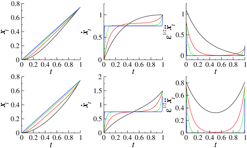
Figure 2: (Color online) Average position ${\boldsymbol{x}}_{t}$, velocity $\dot{\boldsymbol{x}}_{t}$, normalized acceleration $\sqrt{\varepsilon}\,\ddot{\boldsymbol{x}}_{t}$ as obtained from (33), for a time interval $[0,1]$, $x=-0.1$, $\sigma=3.5$, $\tau=h=1$, and $y_{{t_{\mathrm{f}}}}=1$ (upper panels), $y_{{t_{\mathrm{f}}}}=1.5$ (lower panels). The different curves are for $\varepsilon$: $0.1$ (black curve), $0.01$ (red curve), $0.001$ (green curve) and $0.00001$ (blue curve).

Furthermore, for any small but finite $\varepsilon$ our regularization unambiguously determines through (8), (9) the control potential $V$ ($\boldsymbol{b}_{t}=\partial_{\boldsymbol{\xi}_{t}}V$) in the closed control interval $\mathbb{I}$. This means that for any $\varepsilon\,>\,0$ the optimal work expression

$$\mathcal{W}_{\star}=\mathrm{E}\left\{U_{\mathrm{f}}-U_{\mathrm{o}}+\ln\frac{\rho_{{t_{\mathrm{f}}}}}{\rho_{{t_{\mathrm{o}}}}}\right\}+\mathcal{A}_{\star}$$ (32)

is well defined. In particular, for transformations between equilibrium Gaussian sates we have immediately $\mathcal{W}_{\star}=\mathcal{Q}_{\star}$.

Finally, we consider the minimization of (22) under the hypothesis that the final state is still Gaussian but out of equilibrium. In particular, we suppose the final value of the control potential $U_{\mathrm{f}}=c\,|\boldsymbol{x}-\boldsymbol{h}|^{2}/2$ to differ from the osmotic (equilibrium) potential $\ln[\rho_{f}\left(2\,\pi\,\sigma^{2}/\beta\right)^{d/2}]=-|\boldsymbol{x}-\boldsymbol{\mu}|^{2}/2\sigma^{2}$, thus implying a non-vanishing final current velocity. Proceeding as before we obtain

$$\dot{\boldsymbol{x}}_{t}=G_{\boldsymbol{\lambda}}\sinh\left(\!\frac{t-{t_{\mathrm{o}}}}{\sqrt{\varepsilon}\tau}\!\!\right)+\frac{\boldsymbol{\lambda}}{2\tau}\!\left[\!\cosh\left(\!\frac{t-{t_{\mathrm{o}}}}{\sqrt{\varepsilon}\tau}\!\!\right)\!-1\!\right]\ ,$$ (33)

with $G_{\boldsymbol{\lambda}}=[2\tau\boldsymbol{y}_{{t_{\mathrm{f}}}}-\boldsymbol{\lambda}(c_{\boldsymbol{\lambda}}-1)]/2\tau s_{\boldsymbol{\lambda}}$ and where, to ease notation, $s_{\boldsymbol{\lambda}}=\sinh\left(\Delta t/\sqrt{\varepsilon}\tau\right)$, $c_{\boldsymbol{\lambda}}=\cosh\left(\Delta t/\sqrt{\varepsilon}\tau\right)$, and

$$\boldsymbol{\lambda}=\frac{c_{\boldsymbol{\lambda}}+1}{s_{\boldsymbol{\lambda}}}\frac{\boldsymbol{y}_{{t_{\mathrm{f}}}}\sqrt{\varepsilon}\tau(c_{\boldsymbol{\lambda}}\!-\!1)-(\boldsymbol{\mu}+\boldsymbol{x}_{\mathrm{o}}\,(\sigma\!-\!1))s_{\boldsymbol{\lambda}}}{(\Delta t/2\tau)(c_{\boldsymbol{\lambda}}+1)-\sqrt{\varepsilon}s_{\boldsymbol{\lambda}}}\ .$$ (34)

In the limit of vanishing regularization the minimal work done on the system to operate the transformation tends to

$$\mathcal{W}_{\star}\overset{\varepsilon\downarrow 0}{\to}\left(\frac{c\,d\,\sigma^{2}}{2\,\beta}+\frac{c\,\parallel\boldsymbol{\mu}-\boldsymbol{h}\parallel^{2}}{2}\right)+\mathcal{Q}_{\star}(\boldsymbol{\mu},\sigma)$$ (35)

whilst within the open interval $({t_{\mathrm{o}}},{t_{\mathrm{f}}})$ the mean state of the system changes linearly as $\boldsymbol{x}_{t}=\boldsymbol{x}+(t-{t_{\mathrm{o}}})[\boldsymbol{\mu}+\boldsymbol{x}\,(\sigma-1)]/\Delta t$ independently of the final value of the current velocity $\boldsymbol{y}_{tf}$. We illustrate this phenomenon in Fig. 2.

From (35) we can determine the Gaussian nonequilibrium state which, given the final value of the control potential $U_{f}$, minimizes the work. A straightforward calculation shows that the minimum is attained for $\boldsymbol{\mu}=c\,\Delta t\,\boldsymbol{h}/(c\,\Delta t+2\,\tau)$ and $\sigma^{-2}=[\sqrt{\Delta t\,(c\,\Delta t+2\,\tau)+\tau^{2}}-\tau]^{2}/(\Delta t)^{2}$. Thus, we recover the result of SS07 ; Aurell2011 for the minimal work transforming an initial equilibrium state under the constraint that the protocol at the end of the control horizon should attain an assigned final value. Our regularization framework allows us to interpret such work as lower bound over the work done between given states positing that it is possible to retain knowledge of the final protocol but the knowledge on the final non-equilibrium state is lost.

In summary, we have investigated optimal control in stochastic thermodynamics. First, we have shown that the optimal control equations for heat and work transformations between given states have a natural interpretation in terms of functionals definite under time reversal of the Markov process describing the overdamped dynamics. Second, we have proposed a regularization framework in terms of current acceleration. The regularization allows us to identify without ambiguities the internal energy of the system with the drift potential. In the limit of vanishing regularization, the current acceleration tends to zero within the control horizon but diverges (as $\varepsilon^{-1/2}$ in the examples considered) at the control-horizon end-times thus carrying no contribution to the heat release. Correspondingly, the optimal protocol converges toward the overdamped solution by forming boundary layers i.e. regions of faster variation at the control horizon boundaries. As $\varepsilon$ vanishes, these regions shrink to measure zero sets over which the internal energy forms in the limit discontinuities bringing finite contributions to the work done on the system during the transformation. In conclusion we achieved a fully-consistent theoretical picture of optimal overdamped thermodynamics well suited for the interpretation of experimental and numerical data.

This work supported by the Swedish Research Council through Linnaeus Center ACCESS and the FEDORA program grant 129024 of the Academy of Finland (E.A.), by the center of excellence “Analysis and Dynamics Research” of the Academy of Finland (P.M.G.). The authors gratefully acknowledge the hospitality of NORDITA where part of this work has been done during their stay within the framework of the “Foundations and Applications of Non-Equilibrium Statistical Mechanics” program.

References

• (1) C. Bustamante, J. Liphardt, and F. Ritort, Physics Today 58, 43 (2005)
• (2) R. D. Astumian, J. Chem. Phys. 126, 111102 (2007)
• (3) J. P. Nilmeier, G. E. Crooks, D. D. L. Minh, and J. D. Chodera, Proceedings of the National Academy of Sciences(2011), doi:“bibinfo–doi˝–10.1073/pnas.1106094108˝
• (4) T. Schmiedl and U. Seifert, Phys. Rev. Lett. 98, 108301 (2007)
• (5) A. Gomez-Marin, T. Schmiedl, and U. Seifert, J. Chem. Phys. 129, 024114 (2008)
• (6) H. Then and A. Engel, Phys. Rev. E 77, 041105 (2008)
• (7) P. Geiger and C. Dellago, Phys. Rev. E 81, 021127 (2010)
• (8) E. Aurell, C. Mejía-Monasterio, and P. Muratore-Ginanneschi, Phys. Rev. Lett. 106, 250601 (2011)
• (9) E. Nelson, Dynamical Theories of Brownian Motion, Mathematical Notes (Princeton University Press, 1967)
• (10) E. Nelson, Quantum Fluctuations (Princeton University Press, 1985)
• (11) K. Sekimoto, Prog. Theor. Phys. Suppl. 180, 17 (1998)
• (12) R. Durrett, Stochastic calculus: a practical introduction, Probability and stochastics series (CRC Press, 1996) p. 341