Optimization of Connection Patterns between Mobile Phones and Base Stations using Quantum Annealing

Abstract

In current mobile networks, optimizing which base station a mobile phone in a particular area connects to is crucial for ensuring good communication quality for each mobile phone but presents a challenging combinatorial optimization problem. In this study, we optimize the connection patterns to base stations using quantum annealing which is a generic solver using quantum fluctuation. However, since the number of qubits on a quantum annealer is limited, it is necessary to consider a formulation that efficiently utilizes qubits. By adopting a variable reduction formulation, we significantly reduce the qubit requirements compared to the naive formulation that is typically used when considering pattern-matching problems. Furthermore, experiments using quantum annealing revealed that the accuracy of the approximate solution obtained by the new formulation is superior to that of the conventional formulation. Additionally, we demonstrate that the new formulation provides better solutions than the conventional formulation as the problem size increases, even when using simulated annealing, the classical counterpart of quantum annealing.

Introduction

Each base station adjusts its coverage area in modern mobile networks, but controlling it according to traffic conditions is challenging. When many mobile phones connect to a single base station while there are multiple base stations in the neighborhood, there can be an imbalance in the frequency and power usage among base stations. Therefore, in areas with many mobile phones and multiple base stations, it is necessary to optimize the connection patterns between each phone and base station to ensure communication quality for all mobile phones. Various studies have been conducted on optimizing such connection patterns[1].

However, as the number of mobile phones and base stations increases, the number of possible solutions grows exponentially, making the problem difficult to solve. Recently, quantum annealing (QA), a method based on the principles of quantum mechanics[2], has gained attention as a general approach to solving such combinatorial optimization problems. Quantum annealing searches for the ground state of an Ising model, and since many combinatorial optimization problems can be reduced to finding the ground state of an Ising model[3], it can be used to solve a wide range of combinatorial optimization problems such as traffic light control[4, 5, 6], manufacturing[7, 8], finance[9, 10], steel manufacturing[11], and algorithms in machine learning[12, 13, 14, 15, 16, 17]. With these backgrounds, QA has recently attracted attention. In this study, we apply QA to optimize connection patterns and demonstrate that QA can be applied to optimization problems in the wireless communication field.

The quantum annealer, developed by D-Wave Systems, is a representative example of a quantum annealer that implements QA. However, the number of qubits on the D-Wave quantum annealer is still insufficient to solve large-scale real-world problems. Moreover, quantum annealers like the D-Wave quantum annealer can only handle optimization problems formulated as quadratic unconstrained binary optimization (QUBO)[18], equivalent to the Ising model. Therefore, combinatorial optimization problems must be formulated as QUBO to be solved. However, qubits are not fully interconnected on the hardware of the D-Wave quantum annealer, so it is not always possible to map logical variables directly onto qubits. If the graph representing the logical variables and their interactions is dense, it may require multiple qubits to represent a single logical variable on the hardware graph, a technique known as minor embedding. When using the D-Wave quantum annealer, this embedding process often increases the number of qubits required compared to the number of logical variables. Therefore, developing a QUBO formulation that minimizes the required number of qubits is necessary.

A new QUBO formulation that reduces the number of qubits has been proposed in the context of evacuation optimization[19]. In evacuation optimization, the problem is to decide which shelter to assign evacuees to within an evacuation area, given the distance from their current location to each shelter and the capacity limits of the shelters. Each evacuee should be assigned to the closest shelter, but due to capacity constraints, not all evacuees can go to their closest shelter. However, evacuees can not always take a long way to shelter to rigorously satisfy the capacity constraints. In addition, the quantum annealer does not have enough capability to optimize the cost function with several strong coefficients, as in the penalty method. The new formulation thus omits the penalty method and takes binary selection, i.e., the closest or the second one. As a result, the new formulation proposed for this problem effectively reduces the number of required qubits, allowing larger problems to be addressed on the D-Wave quantum annealer than the naive formulation used for assignment problems.

Recognizing the similarity between the evacuation optimization problem and our problem of optimizing connection patterns to base stations, we employ this new QUBO formulation to address our problem. We show that this proposed formulation reduces the number of qubits needed for embedding the QUBO and improves the accuracy of the solutions obtained from the D-Wave quantum annealer. Furthermore, we confirm that the proposed formulation provides better solutions as the problem size increases, even when using simulated annealing (SA)[20], the classical counterpart of quantum annealing. The results suggest that the proposed formulation yields more accurate approximate solutions as the problem size increases, even when using classical QUBO solvers like SA.

The remainder of this paper is organized as follows. In the next chapter, we describe the problem setting for optimizing connection patterns to base stations, including the settings for radio waves emitted from the base stations and the optimization metrics. We introduce both a naive QUBO formulation for connection pattern optimization and a new QUBO formulation in Chapter 3. In Chapter 4, we present the results of comparing the two formulations regarding the number of qubits required and the accuracy of the solutions obtained on the D-Wave quantum annealer. We also investigate the results of comparing the formulations using SA. Finally, Chapter 5 discusses the experimental results and future research directions.

Problem Setting

This chapter describes the problem setting for optimizing connection patterns between mobile phones and base stations. As shown in Fig. 1, we consider a situation where the positions of mobile phones and base stations are fixed within a certain area.

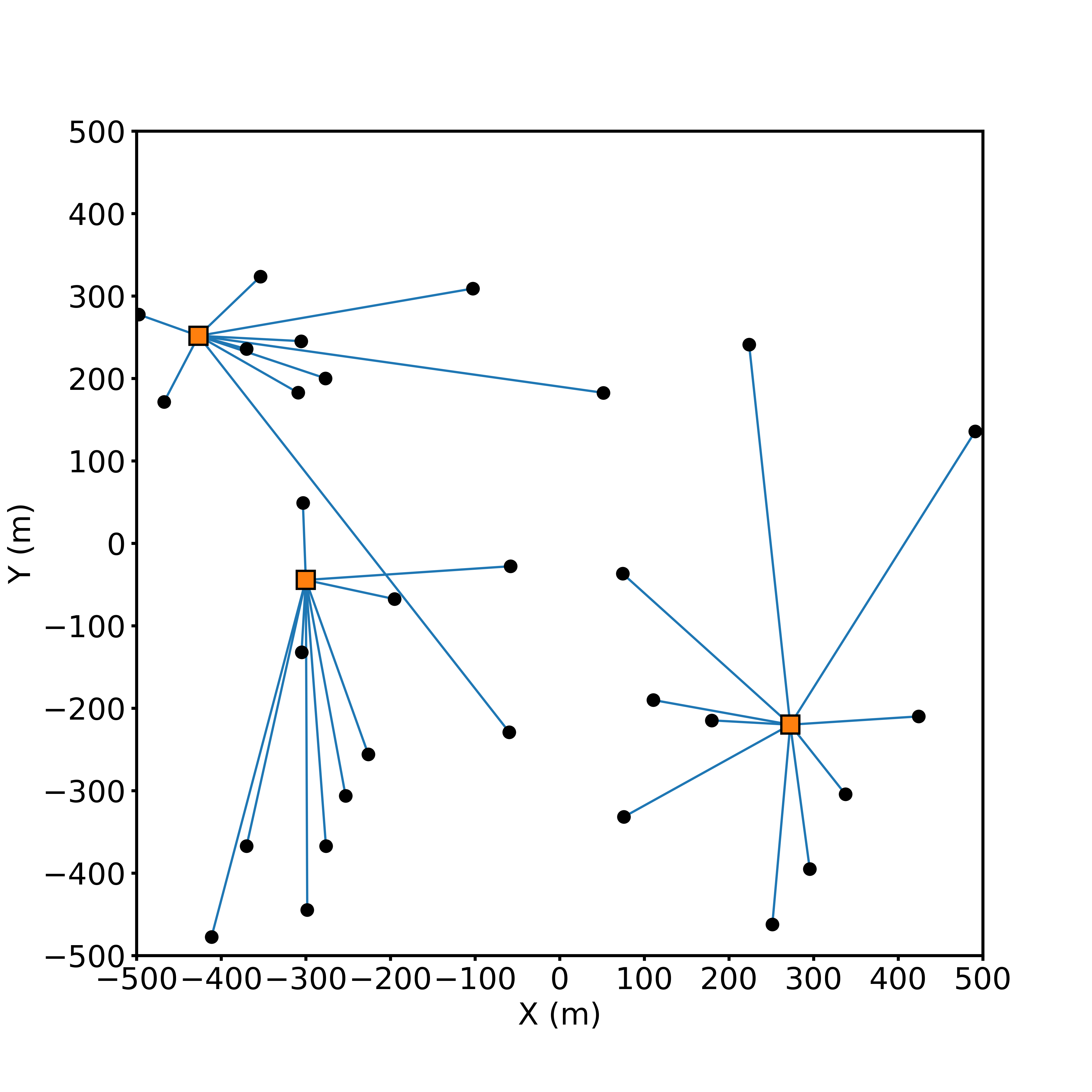
Figure 1: Example of a connection pattern between base stations and mobile phones. Orange squares represent base stations, and black circles show mobile phones. The blue line illustrates the connection between each mobile phone and its corresponding base station.

There are two constraints for determining the connection pattern. The first constraint is that each mobile phone must connect to one of the base stations to enable communication. The second constraint is that each base station has a connection limit to prevent overcrowding at certain base stations. Under these two constraints, we aim to connect each mobile phone to a base station that maximizes communication quality which is defined next.

In this study, we use the down-link signal-to-interference-and-noise ratio (DL-SINR) as the metric of communication quality for each mobile phone. The following equation expresses DL-SINR:

$${\rm DL-SINR}=\frac{S}{I+N},$$ (1)

where $S$ is the desired signal strength, $I$ is the interference signal strength, and $N$ is the noise signal strength. The desired signal strength is the strength of the received signal from the base station to which the mobile phone is connected. The interference signal strength is the sum of the received signal strengths from all other base stations. DL-SINR indicates how a mobile phone can receive data, with higher values representing better communication quality. This paper only considers the down-link, so we refer to DL-SINR simply as SINR.

The following equation calculates the received signal strength:

$${\rm Received\ Signal\ Strength}=\frac{({\rm Transmission}\ {\rm Power})\times({\rm Transmission\ Antenna\ Gain})\times({\rm Received\ Antenna\ Gain})}{\rm Path\ Loss}.$$ (2)

This study assumes the received antenna gain is a constant value of 1. Since the same transmit power is used for all cases, it will be omitted in subsequent calculations. Therefore, the received signal strength is calculated based on the path loss and Transmission antenna gain. Path loss is given by the free space path loss (FSPL) as follows:

$${\rm FSPL}=\left(\frac{4\pi df}{c}\right)^{2},$$ (3)

where $\pi$ is the ratio of the circumference of a circle to its diameter, $d$ is the distance, $f$ is the frequency, and $c$ is the speed of light. FSPL represents the loss when electromagnetic waves travel through space without obstacles. Specifically, it refers to the phenomenon where electromagnetic waves weaken as they travel through space, and it increases as the distance between the mobile phone and the base station increases.

Regarding the Transmission antenna pattern, we consider the following two representative patterns:

Isotropic

The isotropic pattern is an antenna pattern where beams are emitted uniformly in all directions. Fig. 2(a) is a heat map that shows the SINR at each coordinate when two base stations with isotropic patterns are placed 1 km apart, with mobile phones uniformly distributed every meter. All mobile phones at each position connect to the base station that provides the higher SINR. The figure shows that radio waves are emitted uniformly in all directions from the base station in the isotropic pattern, and the SINR decreases with distance from the base station. Therefore, in the isotropic pattern, each mobile phone can obtain a high SINR by connecting to the base station closest to it.

Gaussian

The Gaussian pattern is an antenna pattern with directivity, unlike the isotropic pattern. The gain $G(\phi)$ of the Gaussian pattern is calculated as follows, where $\phi$ is the azimuth angle:

$$G(\phi)=\max\{G_{\rm main}(\phi),{\rm SLL}\}.$$ (4)

Here, $G_{\rm main}(\phi)$ denotes the main beam level, while SLL stands for the side lobe level. The main beam level refers to the peak gain of the antenna pattern, which corresponds to the maximum radiation intensity. On the other hand, the sidelobe level represents the radiation intensity in directions other than the main beam, and it is typically weaker than the main beam level. $G_{\rm main}$ can be written as follows, where $G_{\rm max}$ is the maximum gain:

$$G_{\rm main}(\phi)=\exp\left\{-\frac{1}{2}\left(\frac{\phi}{\sigma}\right)^{2}\times 10^{\frac{G_{\rm max}}{10}}\right\}.$$ (5)

Here, $\theta$ is the half-power beam width, and its relationship with $\sigma$ is as follows:

$$\theta=\frac{\sigma}{2\sqrt{\ln{2}}}.$$ (6)

Fig. 2(b) is the heat map that shows the SINR at each coordinate when two base stations with Gaussian patterns are placed 1 km apart, with mobile phones uniformly distributed every meter. All mobile phones at each position connect to the base station that provides the higher SINR. The half-power beam width is 30 degrees, the maximum gain is 0 dB, and the side lobe level is -15 dB. The figure shows that in the Gaussian pattern, radio waves are emitted with directivity toward several directions from the base station, and mobile phones can obtain a high SINR by connecting to the base station whose beam is directed toward them, rather than simply connecting to the nearest base station.

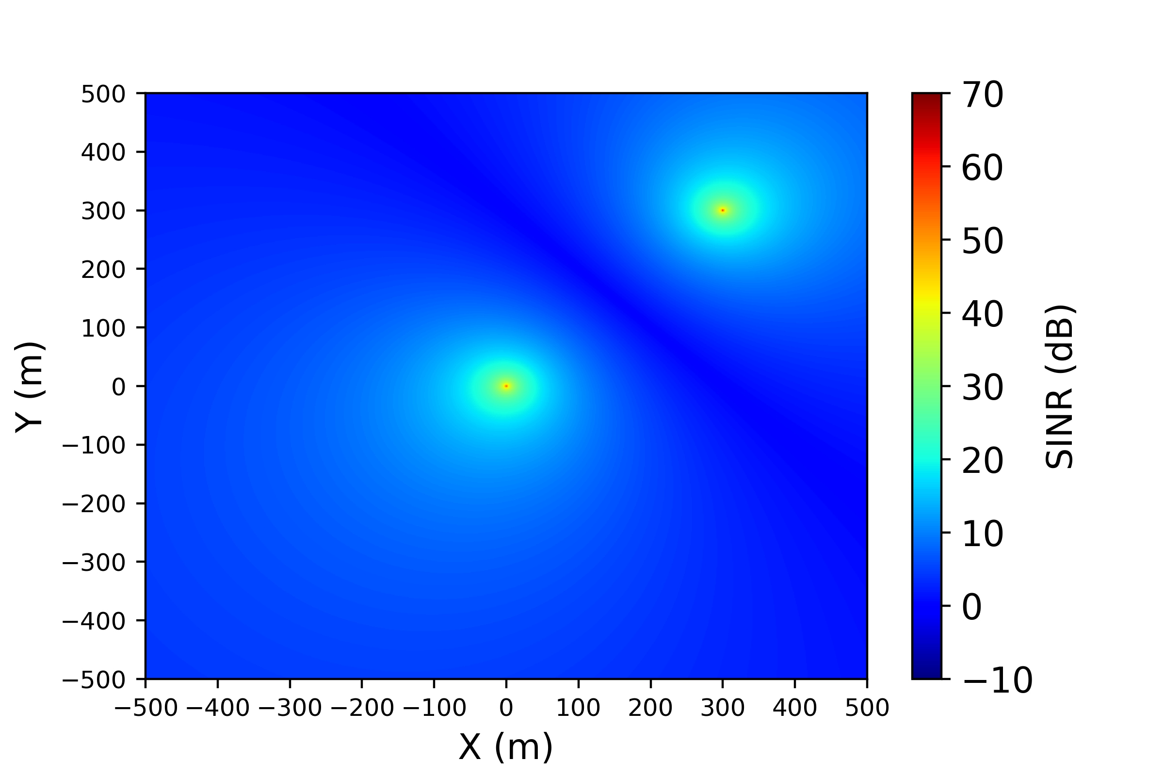
(a) isotropic

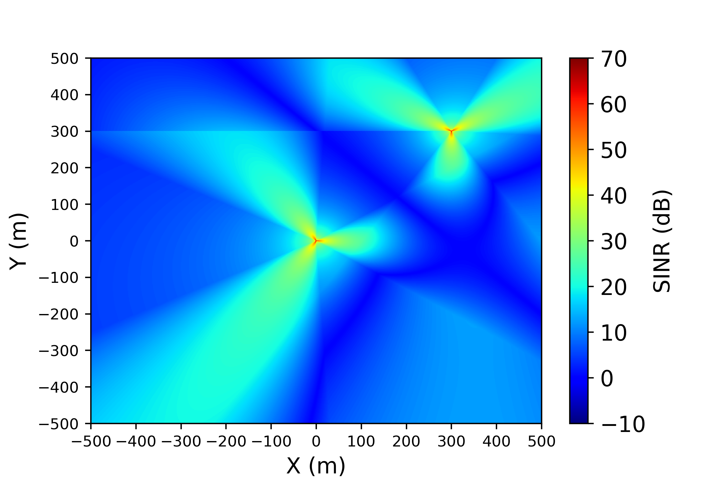
(b) Gaussian

Figure 2: Two Transmission antenna patterns. Each heat map shows the SINR at each coordinate when the base station is located at (0, 0) and (350, 350).

In connection pattern optimization, we aim to maximize the SINR received by each mobile phone within the area. However, since connection limits exist on the base stations, not all mobile phones can connect to the base station that provides the highest SINR. Therefore, this capacity constraint must be included in the formulation. The next chapter introduces two QUBO formulations for connection pattern optimization. The first is a naive formulation commonly used for considering pattern-matching. The second applies the QUBO formulation proposed in the previous study[19], which reduces the number of qubits required by focusing on the top two best connections for each mobile phone.

Method

Naive formulation

In this section, we describe the naive formulation for the problem of maximizing the SINR of each mobile phone when the positions of mobile phones and base stations and the antenna patterns are fixed. This problem involves determining which mobile phone should connect to which base station. In such cases, the decision variables are generally defined as follows:

$${x_{i,a}=}\left\{\,\begin{aligned} &1\quad{\rm if}\quad{\rm mobile\ phone}\ i\ {\rm connects\ to\ base\ station}\ a.\\ &0\quad{\rm otherwise}.\end{aligned}\right.$$ (7)

By using these variables, we can write the problem that maximizes the sum of the SINR of each mobile phone as follows:

$$\max_{x}\quad\sum_{i=1}^{N}\sum_{a=1}^{M}S_{i,a}x_{i,a},$$ (8a)

$${\rm s.t.}\quad\sum_{a=1}^{M}x_{i,a}=1,\quad\forall i\in\{1,\cdots,N\},$$ (8b)

$${\rm s.t.}\quad\sum_{i=1}^{N}x_{i,a}=C_{a},\quad\forall a\in\{1,\cdots,M\},$$ (8c)

where $N$ is the number of mobile phones, $M$ is the number of base stations, $S_{i,a}$ is the SINR when mobile phone $i$ connects to base station $a$, and $C_{a}$ is the capacity of base station $a$. Here $S_{i,a}$ can be uniquely calculated from the fixed positions of the mobile phones and base stations. In this paper, we assume $C_{a}=N/M$ for all $a$, meaning that each of the $N$ mobile phones is connected to one of the $M$ base stations. Eq. (8a) represents the objective function, which maximizes the total SINR. Equation (8b) represents a one-hot constraint, indicating that each mobile phone connects to exactly one base station. Equation (8c) denotes the capacity constraint, ensuring that exactly $C_{a}$ mobile phones are connected to each of the $M$ base stations.

To solve the above problem using a quantum annealer, it needs to be formulated as a QUBO problem. In this formulation, the equality constraints expressed by Eqs. (8b) and (8c) are included in the objective function as penalty terms. The resulting QUBO can be expressed as:

$$\min_{x}\quad-\sum_{i=1}^{N}\sum_{a=1}^{M}S_{i,a}x_{i,a}+\lambda_{1}\sum_{i=1}^{N}\left(\sum_{a=1}^{M}x_{i,a}-1\right)^{2}+\lambda_{2}\sum_{a=1}^{M}\left(\sum_{i=1}^{N}x_{i,a}-C_{a}\right)^{2},$$ (9)

Here, $\lambda_{1}$ and $\lambda_{2}$ are hyper-parameters that control the magnitude of the constraints. Since this QUBO formulation considers all possible connection patterns between mobile phones and base stations, if optimized correctly, it can yield the optimal solution. However, solving this naive QUBO using a quantum annealer is not efficient. This formulation requires many logical variables, $N\times M$, as shown in Eq. (7). Furthermore, due to the one-hot constraint (8b), only $N$ of these variables are meaningful, while the remaining $N(M-1)$ variables are redundant. his is not ideal when using a quantum annealer with limited computational resources. To overcome this issue, we introduce a new formulation that effectively reduces the number of logical variables in the next section.

Proposed formulation

We employ a new formulation, originally proposed in the context of evacuation optimization, to effectively reduce the number of logical variables[19]. In evacuation optimization, the problem is to decide which shelter to assign evacuees to within an evacuation area, given the distance from their current location to each shelter and the capacity limits of the shelters. Each evacuee should be assigned to the closest shelter, but due to capacity constraints, not all evacuees can go to their closest shelter. This problem setting is analogous to our problem of optimizing connection patterns, where the "magnitude of the SINR when mobile phone $i$ connects to base station $a$" corresponds to the "smallness of the distance between evacuee $i$ and shelter $a$."

Based on the new formulation proposed in previous research, we define the decision variables as follows:

$${x_{i}=}\left\{\,\begin{aligned} &1\quad{\rm if}\quad{\rm mobile\ phone}\ i\ {\rm connects\ to\ the\ base\ station\ that\ provides\ the\ highest\ SINR}.\\ &0\quad{\rm if}\quad{\rm mobile\ phone}\ i\ {\rm connects\ to\ the\ base\ station\ that\ provides\ the\ second\ highest\ SINR}.\end{aligned}\right.$$ (10)

In this formulation, each mobile phone only has the option to connect to either the best or the second-best base station, and it is not assigned to any base station that provides lower communication quality. This is based on the practical assumption that each mobile phone should ideally be assigned to the best base station, but due to capacity constraints, it may have to settle for the second-best base station. By formulating the problem this way, the one-hot constraint (8b) of the naive formulation becomes unnecessary. Therefore, in the QUBO, we only need to consider the objective function and the capacity constraint, as expressed below:

$$\min_{x}\quad-\sum_{i=1}^{N}\left(S^{{}^{\prime}}_{i,1}x_{i}+S^{{}^{\prime}}_{i,2}(1-x_{i})\right)+\lambda^{{}^{\prime}}\sum_{a=1}^{M}\left(\sum_{i\in N_{1}(a)}x_{i}+\sum_{i\in N_{2}(a)}(1-x_{i})-C_{a}\right)^{2}.$$ (11)

In this formulation, as shown in Eq. (10), the number of logical variables is reduced to $N$. Thus, compared to the naive formulation, the number of logical variables is reduced to $1/M$, significantly decreasing the number of qubits required in the quantum annealer. In the naive formulation, many of the variables represent $x_{i,a}=0$, which are redundant, whereas, in the proposed formulation, all $N$ variables directly represent the connection choices of the mobile phones, with no waste in variables. Moreover, since each mobile phone is only connected to the best or second-best base station, the proposed formulation is expected to provide a good approximate solution. While the naive formulation, which considers all connection patterns, may yield the optimal solution, the proposed formulation is more efficient regarding qubit usage and will likely provide a good approximate solution quickly, especially considering the error-prone nature of QA with an increasing number of qubits.

In the next chapter, we experimentally compare the effectiveness of the proposed formulation with the naive formulation. Specifically, we compare the number of qubits required and the accuracy of the solutions obtained from the D-Wave quantum annealer for the same problem size in both formulations. Additionally, we used SA instead of D-Wave quantum annealers to investigate the dependence of the accuracy of the solutions obtained by the two formulations on the number of mobile phones.

Experiments

In this chapter, we show the results of the experiments to compare the naive formulation (9) with the proposed formulation (11). As experimental conditions, we randomly distribute mobile phones and base stations within an area. We conduct experiments under two scenarios: one where the distribution of mobile phones is uniform and another where the distribution is biased toward certain base stations. In a biased pattern, 60% of mobile phones are located around one of the $M$ base stations, meaning that for 60% of the mobile phones, the distance to this particular base station is the shortest. Examples of these distribution patterns are shown in Fig. 3.

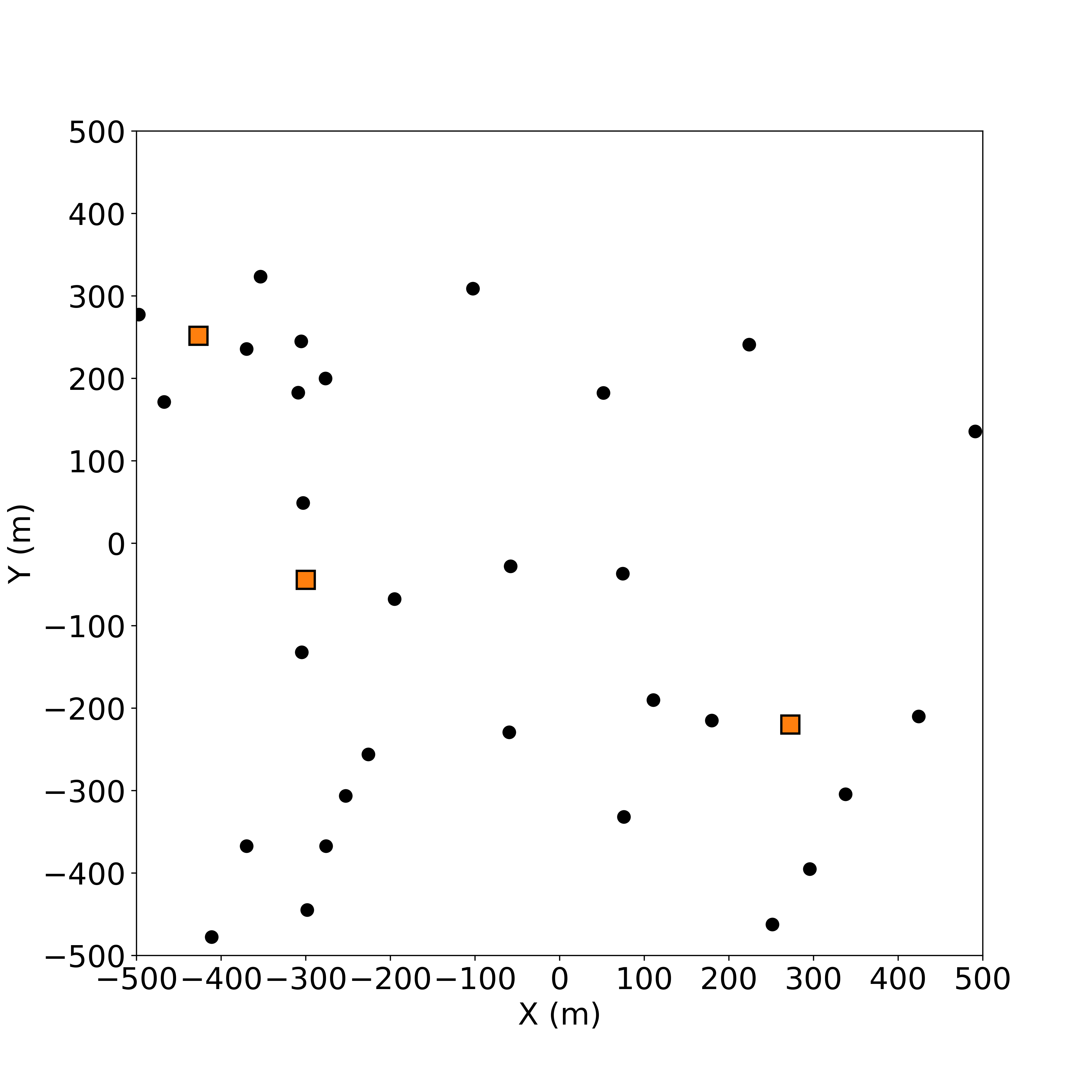
(a) uniform

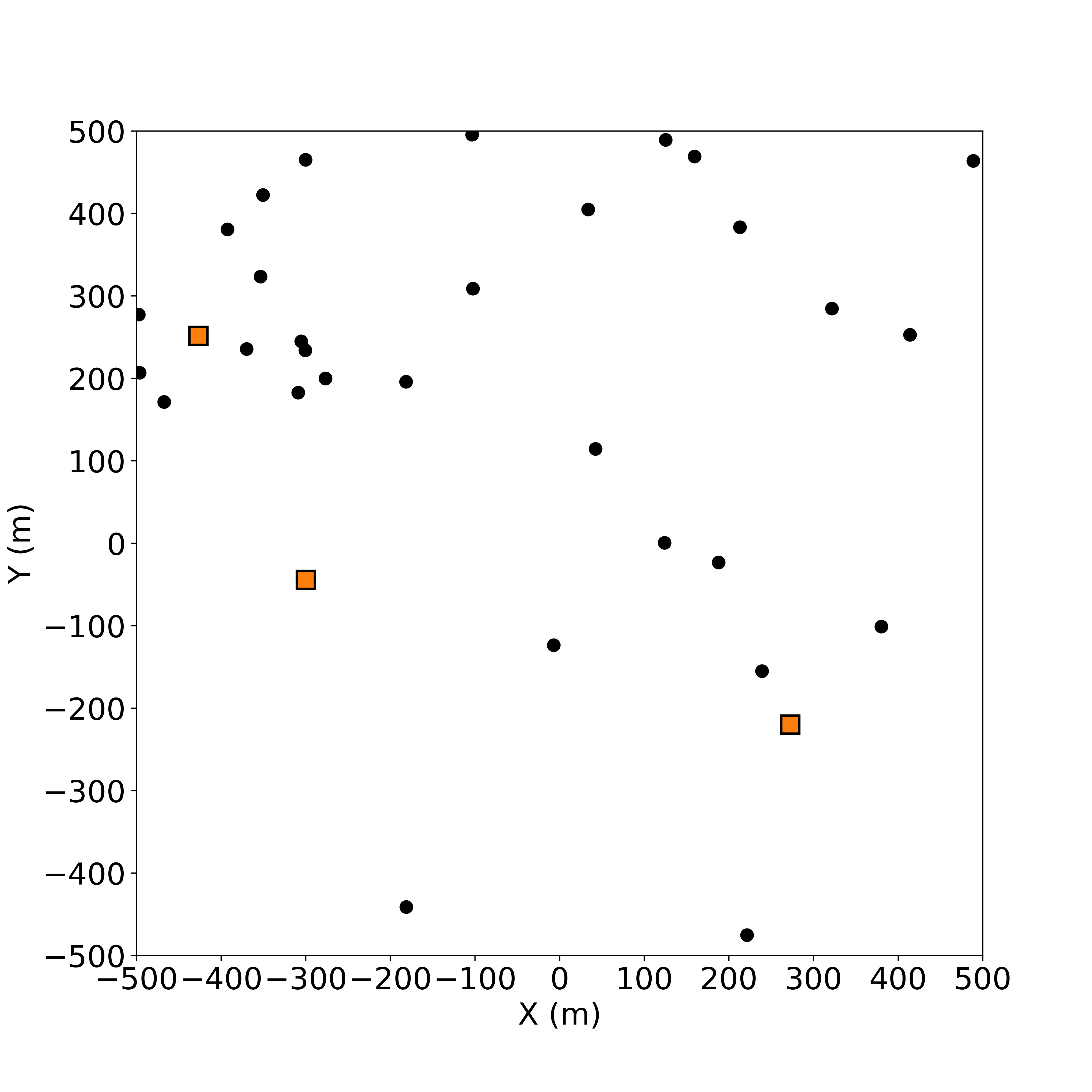
(b) biased

Figure 3: Examples of two mobile phone distribution patterns. The left figure shows a uniform distribution within the area, while the right figure shows a biased distribution towards a specific base station.

In this experiment, we use the isotropic and Gaussian beam patterns shown in Fig. 2. Therefore, we examine four test patterns derived from the combination of mobile phone placement and beam patterns, as shown in Table 1.

Table 1: Four test patterns in experiments.

test pattern	distribution of mobile phones	beam
1	uniform	isotropic
2	biased	isotropic
3	uniform	Gaussian
4	biased	Gaussian

First, we compare the number of qubits required by the two formulations for the same problem size of mobile phones and base stations. The hardware graph for embedding the QUBO is the Pegasus graph installed on the D-Wave Advantage6.4. We use the heuristic library called minorminer [21], provided by D-Wave Systems, for the embedding process. We generate 10 random configurations of mobile phones and base stations and construct QUBOs for each, then compare the number of qubits required. In this experiment, we fix the number of base stations to 3 and examine how the number of required qubits increases with the number of mobile phones. The results are shown in Fig. 4.

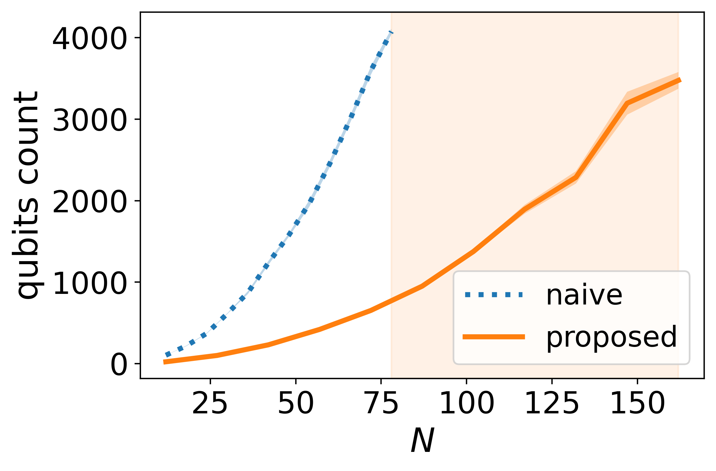
Figure 4: Dependency of the number of qubits required by the two formulations on the number of mobile phones when the number of base stations is fixed at 3. Each line plots the average of 10 instances. The points where the plot is cut off indicate the maximum number of mobile phones $N$ that could be embedded. The area with the orange background highlights the region of $N$ where only the proposed formulation can be embedded.

From Fig. 4, it is clear that the proposed formulation requires fewer qubits than the naive formulation. Additionally, the increase in the number of qubits required as the number of mobile phones increases is smaller in the proposed formulation, allowing it to handle more mobile phones than the naive formulation. Therefore, the proposed formulation is more efficient in using qubits.

Next, we compare the accuracy of the solutions obtained from the D-Wave quantum annealer using the two formulations. We use the D-Wave Advantage 6.4 for QA. We obtained 1000 samples and selected the feasible solution with the lowest cost. The number of mobile phones is fixed at $N=30$, and the number of base stations at $M=3$. We conduct the experiment using the four test patterns shown in Table 1. We create 100 random configurations of mobile phones and base stations for each test pattern and solve each problem on the D-Wave quantum annealer. The results are shown in Fig. 5.

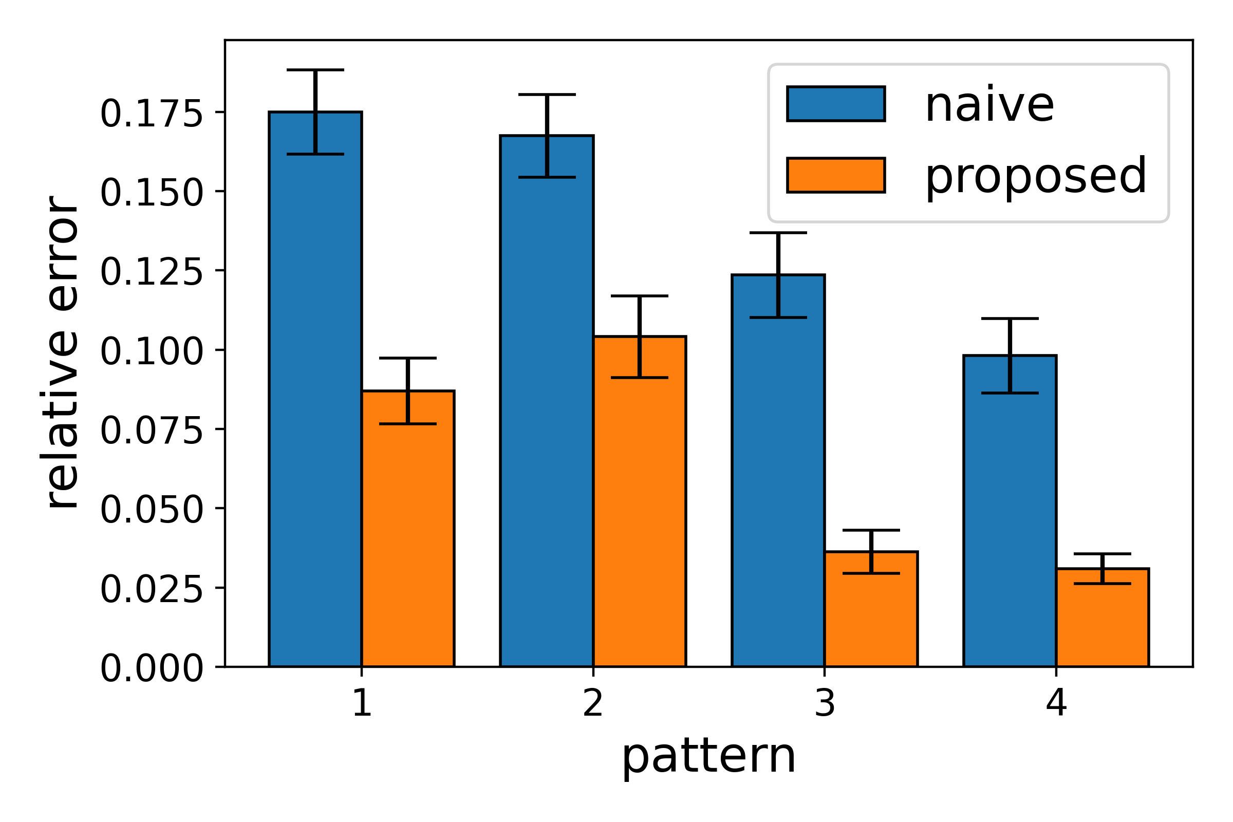
Figure 5: Comparison of the accuracy of solutions obtained using the two formulations across four test patterns.

The horizontal axis in Fig. 5 represents the four test patterns, and the vertical axis represents the relative error $(E-E^{\ast})/E^{\ast}$. Here, $E$ is the cost of the solution $x$ obtained from the quantum annealer, given by $\sum_{i=1}^{N}\left(S^{{}^{\prime}}_{i,1}x_{i}+S^{{}^{\prime}}_{i,2}(1-x_{i})\right)$, and $E^{\ast}$ is the cost of the exact solution $x^{\ast}$ obtained using a exact solver, given by $\sum_{a=1}^{M}S_{i,a}x_{i,a}^{\ast}$. In this experiment, we used the Gurobi optimizer (version 10.0.0) to obtain the exact solution $x^{\ast}$. From Fig. 5, it can be seen that the proposed formulation results in smaller relative errors than the naive formulation in all test patterns. This indicates that the proposed formulation provides more accurate solutions. Additionally, it can be observed that the accuracy is higher when the beam pattern is Gaussian (Test Patterns 3 and 4) compared to when it is isotropic (Test Patterns 1 and 2).

Next, we compare the two formulations when solved using SA and QA. For SA, we used the dwave.neal software (version 0.6.0) provided by D-Wave Systems [22]. The inverse temperature schedule was fixed, and 1000 samples were obtained, selecting the solution with the lowest cost. From the results in Fig. 5, where the proposed formulation outperformed the naive formulation in all test patterns, we focus on Test Pattern 1 in the following experiments. The results are shown in Fig. 6.

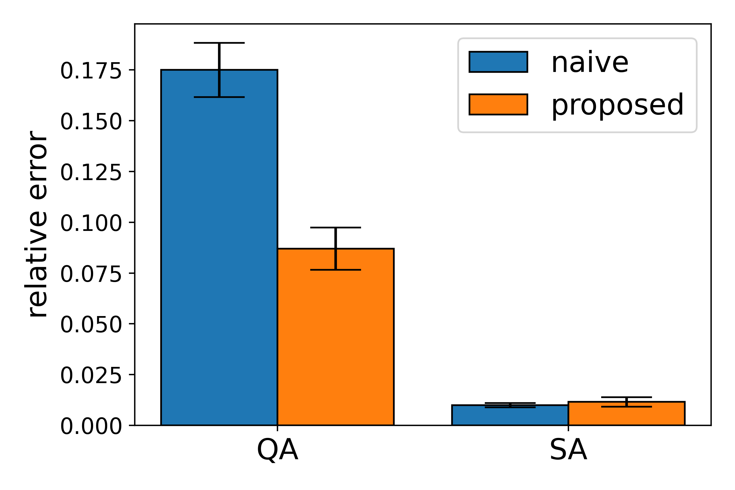
Figure 6: Comparison of the two formulations when solved using SA and QA in Test Pattern 1.

The QA results in Fig. 6 are identical to those in Fig. 5 for test pattern 1. Compared to QA, SA yields significantly lower relative errors for both formulations. This indicates that SA provides more accurate solutions than QA, which is susceptible to errors due to the physical device. On the other hand, unlike QA, the accuracy of the solutions obtained using the two formulations in SA is almost identical. However, this result is specific to the problem size of 30 mobile phones and 3 base stations. Therefore, we next investigate how the accuracy of solutions changes as the number of mobile phones increases in SA for both formulations. In this case, the number of base stations $M$ is fixed at 3, and the SA settings remain the same as in the previous experiment. The results are shown in Fig. 7.

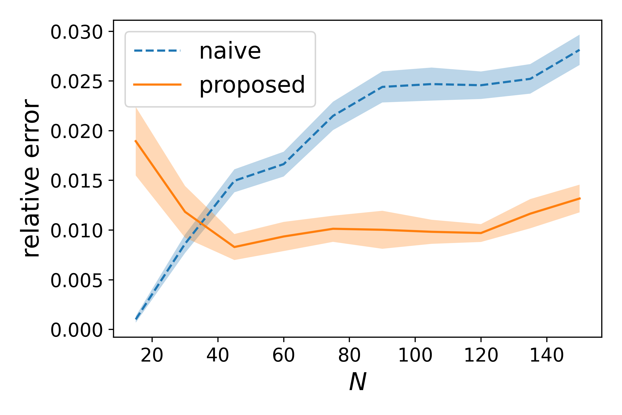
Figure 7: Dependence of the relative error of the two formulations in SA on the number of mobile phones.

From Fig. 7, it can be observed that the naive formulation yields solutions closer to the exact solution when the number of mobile phones is small, but the accuracy deteriorates as the number of variables increases. On the other hand, the proposed formulation maintains good accuracy even as the number of mobile phones increases. Consequently, it can be seen that around $N=30$ to $N=40$, the accuracy of solutions obtained by the two formulations reverses. These results indicate that the proposed formulation provides good approximate solutions in QA and SA as the number of mobile phones increases.

Conclusion

In this study, we conducted experiments comparing the naive formulation (9) with the proposed formulation (11) in the context of optimizing connection patterns of mobile phones to base stations. In the experiment counting the number of qubits shown in Fig. 4, we confirmed that when the number of base stations $M$ is 3, the number of mobile phones that can be handled on the D-Wave Advantage increases. This is because the number of logical variables required by the proposed formulation is reduced to $1/M$ of that required by the naive formulation. By reducing the number of logical variables, the proposed formulation can handle problems with larger mobile phones. These results indicate that the proposed formulation effectively reduces the required qubits.

In the subsequent experiment, as shown in Fig. 5, we compared the accuracy of solutions obtained from the D-Wave quantum annealer across the four patterns listed in Table 1. The results confirmed that the proposed formulation consistently outperforms the naive formulation regarding solution accuracy across all four patterns. The reason for this improvement is likely because, as mentioned above, the proposed formulation reduces the number of logical variables to $1/M$ of that in the naive formulation, reducing the number of qubits required. Since the D-Wave quantum annealer is susceptible to external noise, the more qubits are controlled during QA execution, the greater the likelihood of errors. Therefore, reducing the number of qubits the proposed formulation achieves improves solution accuracy. Thus, the proposed formulation effectively uses limited computational resources on the D-Wave quantum annealer, providing good approximate solutions.

Moreover, as shown in Fig. 7, the proposed formulation also outperforms the naive formulation regarding solution accuracy as the number of mobile phones increases, even when using the classical algorithm SA. As shown by the definition of the variables in Fig. (10), the proposed formulation only considers connecting each mobile phone to either the base station that provides the highest SINR or the second-best base station. Therefore, even if the exact solution to the proposed formulation (11) is obtained, it does not necessarily yield the optimal solution of the original problem described by the naive formulation (8a). As a result, it is understandable that the naive formulation provides better accuracy when the number of mobile phones is small. However, as the number of mobile phones increases, the number of possible solutions increases exponentially, making it a challenging combinatorial optimization problem. Therefore, solving the QUBO based on the naive formulation becomes increasingly difficult with the increase in mobile phones, even in SA, where there is no noise influence as in QA. On the other hand, the proposed QUBO is a simplified problem in which each mobile phone is only connected to the best or second-best base station, enabling stable solutions even as the number of mobile phones increases.

In conclusion, the proposed formulation effectively reduces the number of qubits and improves the accuracy of approximate solutions, making it an efficient approach for utilizing the limited computational resources of quantum annealers. Additionally, even in classical QUBO solvers like SA, the proposed formulation becomes increasingly effective in providing good approximate solutions as the problem size grows.

Future work includes the following considerations. First, the proposed formulation was originally introduced in the context of evacuation optimization. In this study, we applied it to optimize connection patterns to base stations. The key idea of the proposed formulation is to simplify the problem by allowing choices between the best and second-best options, which we believe has potential for various other applications in real-world scenarios. We plan to explore other possible applications of this formulation.

Additionally, while the proposed formulation can reduce the number of qubits required and handle more mobile phones compared to the naive formulation, the number of mobile phones is much larger in real situations. In such cases, it might be necessary to preprocess the data to reduce the number of mobile phones for which connection patterns need to be determined via quantum annealing. We will explore strategies for handling cases with a much larger number of mobile phones.

Finally, in this experiment, we considered a scenario where the positions of the mobile phones are fixed within the area. However, in real-world scenarios, mobile phone positions change over time as people move. Therefore, the connection pattern optimization needs to be repeated periodically. Future work will include simulations that track these temporal changes in mobile phone positions.

Author contributions statement

Takabayashi, T., performed the experiments and analyzed the results. Sudo, S., proposed the research topic and problem formulation and created a calculation tool for problem formulation. Aoki, T., and Seo, S., contributed to refining the research direction, provided input on interpreting the calculation results, and contributed to preparing the manuscript. Ohzeki, M., conceived the idea of the proposed method and supervised this work. All authors participated in discussions of the results and contributed to the final manuscript.

References

- [1] Shen, K., Liu, Y.-F., Ding, D. Y. & Yu, W. Flexible multiple base station association and activation for downlink heterogeneous networks. \JournalTitleIEEE Signal Processing Letters 24, 1498–1502, DOI: 10.1109/LSP.2017.2738027 (2017).
- [2] Kadowaki, T. & Nishimori, H. Quantum annealing in the transverse ising model. \JournalTitlePhys. Rev. E 58, 5355–5363, DOI: 10.1103/PhysRevE.58.5355 (1998).
- [3] Lucas, A. Ising formulations of many np problems. \JournalTitleFrontiers in physics 2, 5 (2014).
- [4] Neukart, F. et al. Traffic flow optimization using a quantum annealer. \JournalTitleFront. ICT 4, 29 (2017).
- [5] Inoue, D., Okada, A., Matsumori, T., Aihara, K. & Yoshida, H. Traffic signal optimization on a square lattice with quantum annealing. \JournalTitleScientific reports 11, 1–12 (2021).
- [6] Shikanai, R., Ohzeki, M. & Tanaka, K. Traffic signal optimization using quantum annealing on real map, DOI: 10.48550/arXiv.2308.14462 (2023). 2308.14462.
- [7] Ohzeki, M., Miki, A., Miyama, M. J. & Terabe, M. Control of automated guided vehicles without collision by quantum annealer and digital devices. \JournalTitleFrontiers in Computer Science 1, 9 (2019).
- [8] Haba, R., Ohzeki, M. & Tanaka, K. Travel time optimization on multi-agv routing by reverse annealing. \JournalTitleScientific Reports 12, 17753, DOI: 10.1038/s41598-022-22704-0 (2022).
- [9] Rosenberg, G. et al. Solving the optimal trading trajectory problem using a quantum annealer. \JournalTitleIEEE J. Sel. Top. Signal Process. 10, 1053–1060 (2016).
- [10] Venturelli, D. & Kondratyev, A. Reverse quantum annealing approach to portfolio optimization problems. \JournalTitleQuantum Machine Intelligence 1, 17–30 (2019).
- [11] Yonaga, K. et al. Quantum Optimization with Lagrangian Decomposition for Multiple-process Scheduling in Steel Manufacturing. \JournalTitleISIJ International 62, 1874–1880, DOI: 10.2355/isijinternational.ISIJINT-2022-019 (2022).
- [12] Amin, M. H., Andriyash, E., Rolfe, J., Kulchytskyy, B. & Melko, R. Quantum Boltzmann Machine. \JournalTitlePhysical Review X 8 (2018). 1601.02036.
- [13] O’Malley, D., Vesselinov, V. V., Alexandrov, B. S. & Alexandrov, L. B. Nonnegative/binary matrix factorization with a d-wave quantum annealer. \JournalTitlePloS one 13, e0206653 (2018).
- [14] Sato, T., Ohzeki, M. & Tanaka, K. Assessment of image generation by quantum annealer. \JournalTitleScientific Reports 11, 13523, DOI: 10.1038/s41598-021-92295-9 (2021).
- [15] Urushibata, M., Ohzeki, M. & Tanaka, K. Comparing the effects of boltzmann machines as associative memory in generative adversarial networks between classical and quantum samplings. \JournalTitleJournal of the Physical Society of Japan 91, 074008, DOI: 10.7566/JPSJ.91.074008 (2022). https://doi.org/10.7566/JPSJ.91.074008.
- [16] Hasegawa, Y., Oshiyama, H. & Ohzeki, M. Kernel learning by quantum annealer, DOI: 10.48550/arXiv.2304.10144 (2023). 2304.10144.
- [17] Goto, T. & Ohzeki, M. Online calibration scheme for training restricted boltzmann machines with quantum annealing, DOI: 10.48550/arXiv.2307.09785 (2023). 2307.09785.
- [18] Glover, F., Kochenberger, G., Hennig, R. & Du, Y. Quantum bridge analytics I: a tutorial on formulating and using QUBO models. \JournalTitleAnnals of Operations Research 314, 141–183, DOI: 10.1007/s10479-022-04634-2 (2022).
- [19] Ohzeki, M. In presentation of Qubits2023.
- [20] Kirkpatrick, S., Gelatt, C. D. & Vecchi, M. P. Optimization by simulated annealing. \JournalTitleScience 220, 671–680, DOI: 10.1126/science.220.4598.671 (1983).
- [21] Cai, J., Macready, W. G. & Roy, A. A practical heuristic for finding graph minors, DOI: 10.48550/arXiv.1406.2741 (2014). 1406.2741.
- [22] D-Wave Systems. Available in https://github.com/dwavesystems/dwave-neal.
Acknowledgments
This study was financially supported by programs for bridging the gap between R&D and IDeal society (Society 5.0) and Generating Economic and social value (BRIDGE) and Cross-ministerial Strategic Innovation Promotion Program (SIP) from the Cabinet Office.