Online calibration scheme for training restricted Boltzmann machines with quantum annealing

Abstract

We propose a scheme for calibrating the D-Wave quantum annealer’s internal parameters to obtain well-approximated samples to train a restricted Boltzmann machine (RBM). Empirically, samples from the quantum annealer obey the Boltzmann distribution, making them suitable for RBM training. However, it is hard to obtain appropriate samples without compensation. Existing research often estimates internal parameters, such as the inverse temperature, for compensation. Our scheme utilizes samples for RBM training to estimate the internal parameters, enabling it to train a model simultaneously. Furthermore, we consider additional parameters beyond inverse temperature and demonstrate that they contribute to improving sample quality. We evaluate the performance of our scheme by comparing the Kullback-Leibler divergence of the obtained samples with classical Gibbs sampling. Our results indicate that our proposed scheme demonstrates performance on par with Gibbs sampling. In addition, the training results with our estimation scheme are better than those of the Contrastive Divergence algorithm, known as a standard training algorithm for RBM.

Introduction

Deep neural networks are now widely studied due to their excellent practical performance. As a part of the deep neural networks, restricted Boltzmann machines (RBMs) can be utilized for unsupervised and supervised tasks, such as facial recognition[1, 2], natural language understanding[3], predictions of electricity loads and degradation of manufacturing facilities[4, 5].

An RBM is trained by minimizing the Kullback-Leibler (KL) divergence between the model distribution and an empirical distribution composed of training data[6]. Training an RBM requires statistical mean values of samples generated by the RBM. Although Gibbs sampling is commonly used to achieve this, it incurs a high computational cost for a long equilibration time. The Contrastive Divergence (CD) algorithm is frequently applied to address this[7]. While not guaranteed to yield accurate results, this scheme can estimate the RBM’s parametric gradient with fewer costs than Gibbs sampling.

As an alternative to the aforementioned schemes, the quantum annealing (QA)[8] approach has attracted attention for its ability to sample from a physical device directly. QA controls the strength of the transverse field in an adiabatic process, wherein the initial state of superposition changes to low-energy states of the final user-designed Hamiltonian. QA has been mainly studied as a solution for optimization where it works by searching for the ground state of the Ising model[9], as in traffic flow optimization[10, 11, 12], finance [13, 14, 15], logistics [16, 17], manufacturing [18, 19, 20], preprocessing in material experiments[21], marketing [22], and decoding problems [23, 24]. Its potential for solving optimization problems with inequality constraints has been enhanced [25], particularly in cases where the direct formulation is challenging[26]. A comparative study of quantum annealer was performed for benchmark tests to solve optimization problems [27]. The quantum effect on the case with multiple optimal solutions has also been discussed [28, 29]. As the environmental effect cannot be avoided, the quantum annealer is sometimes regarded as a simulator for quantum many-body dynamics [30, 31, 32]. Furthermore, applications of quantum annealing as an optimization algorithm in machine learning have also been reported [33, 34, 35, 36, 37, 38, 39, 40, 41].

While quantum annealing effectively solves optimization problems, its application in Boltzmann machine learning has also been established. Empirical evidence supports the assertion that the distribution of samples obtained from the quantum annealer closely approximates the Boltzmann distribution. Accordingly, several studies have demonstrated its application to the training of Boltzmann machines [42, 43, 44, 45]. Some of them[42, 43] have reported results superior to those of the CD algorithm and faster than those of the Gibbs sampling.

Obtaining appropriate samples without calibration is difficult because of hardware imperfections, such as chain breaks and working temperature. To address this, the inverse temperature $\beta_{\rm{eff}}$ of the generated samples is often estimated as a way to compensate the parameters of couplings and fields that are mapped to the quantum annealer. Adachi et al.[42] determined the best fit $\beta_{\rm{eff}}$ that minimizes the error of interaction term of visible and hidden nodes prior to model training. This scheme can not follow the temporal variation of $\beta_{\rm{eff}}$. As a simple approach, Dixit et al.[43] trained models with multiple values of $\beta_{\rm{eff}}$ and adopted the best result. However, such an approach wastes significant computational resources to train models that would remain unused. To handle these problems, several studies[44, 45] have estimated the parameter in the model training process. Benedetti et al.[44] derived a relationship among the difference of probabilities, the energies, and the $\beta_{\rm{eff}}$ of two samples. They then used the relationship and linear regression to approximate $\beta_{\rm{eff}}$. This approach requires post-processing during each iteration, which also impacts training time. The estimation scheme of Xu et al.[45] infers $\beta_{\rm{eff}}$ by maximizing the likelihood. However, the computational cost incurred by this approach is also impractical, as it must calculate the average value over all configurations of the RBM. Although this is not specified clearly, we assume that Gibbs sampling is employed for the approximation, further increasing the training time.

Our method uses samples from a quantum annealer as training data and applies the CD algorithm to estimate internal parameters. CD algorithms have minimal impact on the total training time because they do not require significant computational resources. The samples are effectively used to train the model and approximate the parameters simultaneously. In addition, we introduce three patterns of assumptions with regards to internal parameters: (i) one inverse temperature as in aforementioned methods, (ii) three inverse temperatures for weights, biases of visible units, and biases of hidden units, (iii) one inverse temperature for weights, and a coefficient for each bias.

The remaining part of this paper consists of the following sections. The next section presents the update rule for estimated internal parameters and a detailed algorithm for inferring them during training. In the subsequent section, we showcase the experiments’ results using the D-Wave 2000Q to generate samples. The implemented RBM has 32 visible nodes and 8 hidden nodes. Although it is relatively small, it suffices to validate the proposed scheme. The first half of this section focuses on investigating how the proposed estimation scheme improves sample quality without training. We compare the proposed scheme with conventional Gibbs sampling using histograms and the KL divergence of the samples. We observe that the increased number of internal parameters enhances the sampling quality. In the latter part of this section, we perform a training test to demonstrate the results of our scheme compared to classic schemes. Similar to previous research, our scheme is more accurate than the CD algorithm. The number of internal parameters exhibits the same effect as in the previous experiment.

Methods

Theory of RBM

An RBM consists of a visible layer and a hidden layer denoted as $v=\{v_{1},v_{2},\ldots,v_{n}\}$ and $h=\{h_{1},h_{2},\ldots,h_{m}\}$, respectively. Each layer has stochastic binary variables, and the probability follows a Boltzmann distribution as

$$P({v},{h}|\theta)=\frac{\exp{\left(-E({v},{h}|\theta)\right)}}{Z},$$ (1)

where $\theta$ is the vector of the RBM’s parameters $\{w_{11},\ldots,w_{nm},b_{1},\ldots,b_{n},c_{1},\ldots,c_{m}\}$, $E$ is the energy function expressed as

$$E({v},{h}|\theta)=-\sum_{i,j}w_{ij}v_{i}h_{j}-\sum_{i}b_{i}v_{i}-\sum_{j}c_{j}h_{j},$$ (2)

and $Z$ is the partition function $Z=\sum_{{v},{h}}P(v,h|\theta)$. The RBM is trained by minimizing the KL divergence, expressed as

$$D_{\mathrm{KL}}(Q_{D}||P)=\sum_{v\in\chi}Q_{D}(v)\log\frac{Q_{D}(v)}{P(v|\theta)},$$ (3)

where $\chi$ is a set of all configurations for the visible layer of the RBM, $Q_{D}$ is the empirical distribution of the training data, and $P(v|\theta)$ is a marginal distribution of Eq. (1). Minimizing the KL divergence is equivalent to maximizing the log-likelihood as

$$\mathcal{L}(\theta)=\sum_{v\in{D}}\frac{1}{N_{D}}\log{P(v|\theta)},$$ (4)

where $D$ is the set of training data, and $N_{D}$ is its size. As a result, we obtain the gradient of $\mathcal{L}$ with respect to $\theta$ as

$$\frac{d\mathcal{L}}{d\theta}=\left<\frac{\partial{E}}{\partial\theta}\right>_{D}-\left<\frac{\partial{E}}{\partial\theta}\right>_{\chi},$$ (5)

where $\left<\ldots\right>_{D}$ and $\left<\ldots\right>_{\chi}$ are averages over the training dataset and all configurations for the visible layer, respectively. Each parameter can be updated by using the gradient method according to the following rules:

$$\begin{split}&\delta{w_{ij}}=\eta\left(\left<{v_{i}}{h_{j}}\right>_{D}-\left<{v_{i}}{h_{j}}\right>_{\chi}\right),\\ &\delta{b_{i}}=\eta\left(\left<v_{i}\right>_{D}-\left<v_{i}\right>_{\chi}\right),\\ &\delta{c_{j}}=\eta\left(\left<h_{j}\right>_{D}-\left<h_{j}\right>_{\chi}\right).\end{split}$$ (6)

Calculating the $\left<\ldots\right>_{\chi}$ is difficult because the number of configurations is $2^{n}$. Instead, Gibbs sampling is applied to estimate it. Furthermore, to reduce the calculation cost, the CD algorithm[7] generates samples evolved from the training data instead of calculating $\left<\ldots\right>_{\chi}$. Although these results are not exact, the gradient direction is sufficiently approximated. Consequently, the model can be trained over a single evolution.

Training RBM with quantum annealer

As an alternative to Gibbs sampling, quantum annealing can be used to collect samples for the estimation of $\left<\ldots\right>_{\chi}$ in Eq. (6). Due to the hardware structure, the number of couplings among qubits is limited. Hence, each node in the RBM is embedded in multiple qubits in the quantum annealer. Figure 1 illustrates a sample embedding with D-Wave 2000Q, which has a Chimera graph structure[42].

When a QUBO matrix is determined by Eq. (2), prior studies have assumed[42] that samples from a quantum annealer are obtained as

$$P({v},{h}|\theta,\beta_{\rm{eff}})=\frac{\exp{\left(-\beta_{\rm{eff}}E({v},{h}|\theta)\right)}}{Z_{\beta_{\rm{eff}}}},$$ (7)

where $\beta_{\rm{eff}}$ is an internal parameter of the quantum annealer, and the partition function $Z_{\beta_{\rm{eff}}}$ is $\sum_{{v},{h}}P(v,h|\theta,\beta_{\rm{eff}})$. Samples following Eq. (1) as opposed to Eq. (7) are needed to estimate $\left<\ldots\right>_{\chi}$. Once $\beta_{\rm{eff}}$ is estimated, appropriate samples are generated from the quantum annealer by constructing a QUBO matrix as $E({v},{h}|\theta)/\beta_{\rm{eff}}$ to negate the internal parameter.

As mentioned, most studies have adopted the inverse temperature as an internal parameter. However, as the quantum annealer has many unknown aspects in its hardware, it is unclear whether this correction is sufficient. We formulate the difference between the sample distribution generated by quantum annealing and the original RBM using KL divergence to address this issue. We then minimize this difference to accommodate other patterns of internal parameters. The method proposed below uses the CD algorithm, which requires less calculation, similar to training an RBM.

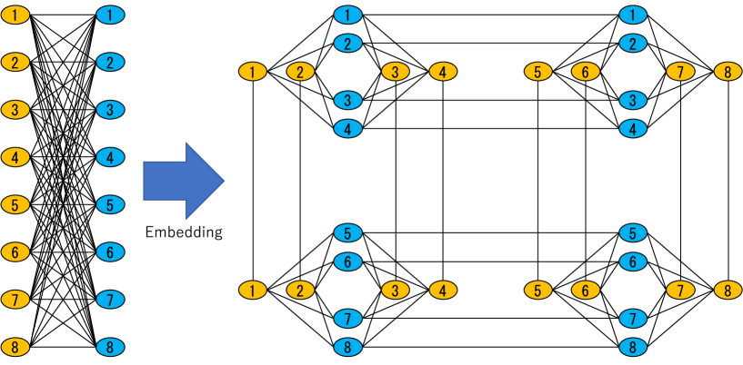
Figure 1: An RBM with a dimension of $8\times 8$, and its embedding to a Chimera graph-based hardware.

Inferring Internal Parameters

Algorithm 1 Algorithm for the estimation of $\beta_{\rm{eff}}$ and training of an RBM

1:Initialize $\theta$ with random values

2:$\beta_{\rm{eff}}\leftarrow 1$

3:while not satisfy the stop condition do

4:     Construct a QUBO matrix from $\theta/\beta_{\rm{eff}}$

5:     Get samples from a quantum annealer with the QUBO matrix

6:     $\beta_{\rm{eff}}\leftarrow$ ESTIMATE_BETA($\beta_{\rm{eff}}$, samples)

7:     Update $\theta$ with training data and return samples

8:end while

1:function estimate_beta($\beta_{\rm{eff}}$,samples)

2:     $\beta_{\rm{tmp}}\leftarrow 1$

3:     $v_{0}\leftarrow$ visible nodes of samples

4:     $h_{0}\leftarrow$ hidden nodes of samples

5:     while not satisfy the stop condition do

6:         $v_{1}\leftarrow$ Carry out Gibbs sampling from all elements of $h_{0}$ according to $P(v|h,\theta,\beta_{\rm{tmp}})$

7:         $h_{1}\leftarrow$ Carry out Gibbs sampling from all elements of $v_{0}$ according to $P(h|v,\theta,\beta_{\rm{tmp}})$

8:         $\beta_{\rm{tmp}}+=\eta\left(\left<E\right>_{v_{0},h_{0}}-\left<E\right>_{v_{1},h_{1}}\right)$

9:     end while

10:     return $\beta_{\rm{eff}}\beta_{\rm{tmp}}$

11:end function

Figure 2: The proposed algorithm. $\left<\ldots\right>_{\chi}$ in Eq. (11) is replaced by an ensemble average of the samples evolved by Gibbs sampling from the return samples owing to the CD algorithm. The stop conditions for loops were specified as 1500 times for training and three times for estimating $\beta_{\rm{eff}}$.

We propose a scheme to infer the internal parameters $\beta$ of a quantum annealer while training an RBM. The scheme uses the return samples from the quantum annealer as training data for estimation, wherein $\theta$ is fixed during estimation. Our objective is to estimate the value of $\beta$ that minimizes the KL divergence between $P(v,h|\theta,\beta)$ and the empirical distribution of the samples $Q_{S}(v,h)$ as

$$D_{\mathrm{KL}}(Q_{S}||P)=\sum_{v,h\in\chi}Q_{S}(v,h)\log\frac{Q_{S}(v,h)}{P(v,h|\theta,\beta)}.$$ (8)

Similar to Eq. (4), this is equivalent to maximizing a log-likelihood:

$$\mathcal{L}(\beta)=\sum_{v,h\in{S}}\frac{1}{N_{S}}\log{P(v,h|\theta,\beta)},$$ (9)

where $S$ is the set of samples and $N_{S}$ is its size. Unlike the case of training an RBM, training data, which are samples from a quantum annealer, include hidden layer bits. Thus, the probability distribution in Eq. (9) is not a marginal distribution of a visible layer. If $\beta_{\rm{eff}}$ in Eq. (7) is assumed as an internal parameter, Eq. (9) becomes

$$\mathcal{L}(\beta_{\rm{eff}})=\frac{1}{N_{S}}\sum_{v,h\in{S}}\beta_{\rm{eff}}E(v,h|\theta)-\log{Z_{\beta_{\rm{eff}}}}.$$ (10)

Therefore, the updating rule for $\beta_{\rm{eff}}$ is derived by differentiating Eq. (10):

$$\delta\beta_{\rm{eff}}=\eta\left(\left<E\right>_{S}-\left<E\right>_{\chi}\right).$$ (11)

The CD algorithm can be used to update $\beta_{\rm{eff}}$ as in the standard training procedure for RBM. The overall algorithm combining estimation of $\beta_{\rm{eff}}$ with training is shown in Fig. 2. Considering that our objective is to obtain samples that have a similar distribution to Eq. (1), we introduce two patterns of internal parameters and distributions:

$$P({v},{h}|\theta,\beta_{vh},\beta_{v},\beta_{h})=\frac{\exp{\left(\beta_{vh}\sum_{i,j}w_{ij}v_{i}h_{j}+\beta_{v}\sum_{i}b_{i}v_{i}+\beta_{h}\sum_{j}c_{j}h_{j}\right)}}{Z_{\beta_{vh,v,h}}},$$ (12)

and

$$P({v},{h}|\theta,\beta_{vh},\beta_{v1},\ldots,\beta_{vn},\beta_{h1},\ldots,\beta_{hm})=\frac{\exp{\left(\beta_{vh}\sum_{i,j}w_{ij}v_{i}h_{j}+\sum_{i}\beta_{vi}b_{i}v_{i}+\sum_{j}\beta_{hj}c_{j}h_{j}\right)}}{Z_{\beta_{vh,vi,hi}}}.$$ (13)

We can derive the update rule for each internal parameter from Eq. (9) similar to Eq. (10) as

$$\begin{split}&\delta{\beta_{vh}}=\eta\left(\left<\sum_{i,j}w_{ij}v_{i}h_{j}\right>_{S}-\left<\sum_{i,j}w_{ij}v_{i}h_{j}\right>_{\chi}\right),\\ &\delta{\beta_{v}}=\eta\left(\left<\sum_{i}b_{i}v_{i}\right>_{S}-\left<\sum_{i}b_{i}v_{i}\right>_{\chi}\right),\\ &\delta{\beta_{h}}=\eta\left(\left<\sum_{j}c_{j}h_{j}\right>_{S}-\left<\sum_{j}c_{j}h_{j}\right>_{\chi}\right),\\ &\delta{\beta_{vi}}=\eta\left(\left<b_{i}v_{i}\right>_{S}-\left<b_{i}v_{i}\right>_{\chi}\right),\\ &\delta{\beta_{hj}}=\eta\left(\left<c_{j}h_{j}\right>_{S}-\left<c_{j}h_{j}\right>_{\chi}\right).\\ \end{split}$$ (14)

The same algorithm can be applied by replacing line 8 in ESTIMATE_BETA of Fig. 2 with corresponding update rules in Eq. LABEL:eq:upd_each_beta. These patterns of internal parameters are hereinafter referred as one-parameter, three-parameter, and one-and-all-bias, respectively. The estimation of many internal parameters requires a large number of samples. Because the proposed method is an online estimation scheme, an increase in internal parameters leads to an increase in estimation time. If we introduce a calibration parameter for each cross term $v_{i}h_{j}$, the increase in parameters is the product of $n$ and $m$, which may significantly increase estimation time. We, therefore, focus on the above three patterns of internal parameters.

Number of samples	Gibbs sampling	One-parameter	Three-parameter	One-and-all-bias
100000	3.49	3.88	3.70	3.64
1000000	1.87	2.46	2.31	2.13

Table 1: KL divergence between empirical distributions of samples and the original RBM.

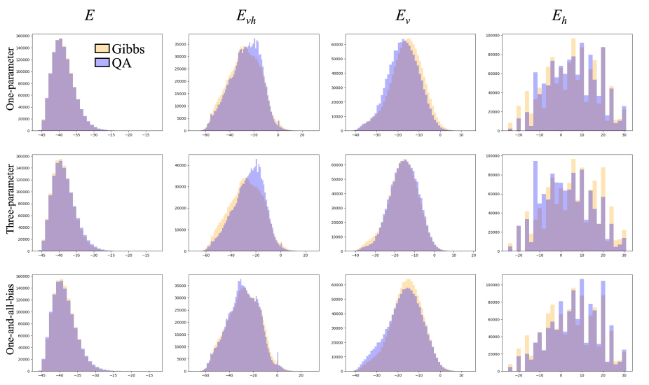
Figure 3: Histograms of samples’ energy. To investigate the effect of internal parameters, we separate the total energy $E$ into $E_{vh}=-\sum{w_{ij}v_{i}h_{j}}$, $E_{v}=-\sum{b_{i}v_{i}}$ and $E_{h}=-\sum{c_{j}h_{j}}$.

Experiments

First, we validated the proposed estimation scheme for the internal parameters without training. The CD algorithm trained an RBM comprising 32 visible nodes and 8 hidden nodes in advance using the coarse-grained MNIST training dataset, similar to prior studies[42]. The same RBM was embedded in 12 locations of D-Wave 2000Q without faulty qubits to gather samples efficiently. We compared samples generated by Gibbs sampling and quantum annealing with those calibrated by the proposed scheme. Table 1 shows the results of KL divergence. The increase in the size of samples decreased KL divergence because the empirical distributions approach the original distribution. In theory, Gibbs sampling can accurately obtain samples following the Boltzmann distribution. Therefore, results close to those obtained by Gibbs sampling can be considered more accurate. We found that the increased number of internal parameters improved sample quality. To determine the reason, Fig. 3 presents histograms of the samples’ energies. Although one parameter can adjust the total energy $E$, the samples’ distributions of $E_{vh}$ and $E_{v}$ exhibit differences between Gibbs sampling and quantum annealing. $E_{v}$ of the three-parameter case and $E_{vh}$ of one-and-all-bias case seem to fit well with Gibbs sampling. Quantum annealers have not only temperature differences, but imperfections of qubits. We consider many internal parameters that can be calibrated to improve sample quality.

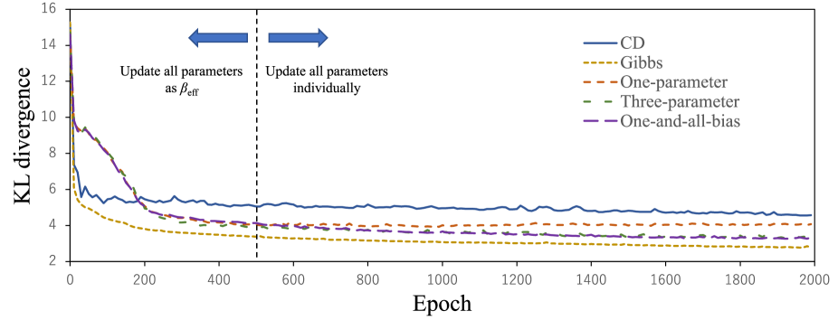
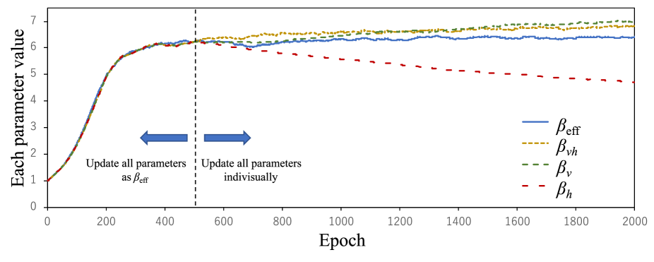
Figure 4: Transition of KL divergence between the empirical distribution of the training data and the trained RBM of each training scheme.

Figure 5: Transition of the estimated internal parameters. We only illustrate the parameters of the one-parameter and three-parameter cases, as there are too many parameters in the one-and-all-bias case.

CD algorithm	Gibbs sampling	One-parameter	Three-parameters	One and all bias
4.56	2.78	3.92	3.30	3.26

Table 2: Minimum KL divergence between the empirical distribution of the training data and the trained RBM of each training scheme.

Next, we conducted RBM training with the simultaneous estimation of internal parameters. The RBM size and training data were identical to the previous experiment. The number of times for updating $\beta$ in each epoch was set to five. The increase in the number of internal parameters enlarges the estimation time. Therefore, all parameters were updated following the same approach as $\beta_{\rm{eff}}$ using Eq. (11) for up to 500 epochs. Then, each parameter was updated with the corresponding update rule. We compare our scheme’s results with the conventional CD algorithm and Gibbs sampling. Figure 5 presents the transition of KL divergence between the empirical distribution of training data and each trained RBM. Table 2 describes the minimum KL divergence in Fig. 5. The results obtained by the proposed algorithm are above those of CD algorithm and below those of Gibbs sampling. The one-and-all-bias case exhibited the best results of the proposed three-parameter configurations, correlating with the previous experimental results. The convergence speed of our scheme slows down just after starting. However, training rapidly progresses between 100 and 200 epochs. We present the estimation results of internal parameters in Fig. 5, indicating that the process accelerates training. As mentioned, all parameters were almost equivalent under 500 epochs as the same update rule was applied. This also indicates that $\beta_{\rm{eff}}$ converges at approximately 500 epochs, leading to the stagnation of KL divergence in the one-parameter case, as illustrated in Fig. 5. On the other hand, the variation of other parameters continued after 500 epochs, and the KL divergence results of two other parametric configurations exhibited continuous improvement. Therefore, these results are better than those of the one-parameter case, revealing that the increase in internal parameters is effective for training. However, whereas $\beta_{\rm{eff}}$ converged early, $\beta_{h}$ did not especially converge. This indicates that the estimation of many internal parameters requires a large number of samples.

Discussion

We propose a novel scheme for estimating the internal parameters $\beta$ of a quantum annealer during the training of an RBM. Our scheme is developed by minimizing the KL divergence between the empirical distribution of samples obtained from the quantum annealer and a Boltzmann distribution constructed using the RBM and $\beta$. Accordingly, the CD algorithm is adopted to infer the parameters. Samples are utilized for both training and estimation simultaneously, which reduces training time compared to conventional schemes. In addition, the proposed algorithm can calibrate multiple internal parameters. Although the inverse temperature is generally estimated as an internal parameter, using additional internal parameters potentially enhances the sample distribution’s accuracy.

Through experimental results, we confirmed that an increased number of internal parameters reduces KL divergence, further contributing to improved training results. The results of the proposed method surpass those of the conventional CD algorithm, as indicated by our results. However, it is important to note that estimating numerous parameters using our method requires a significant amount of time. Additional techniques appear to be required, such as initiating an update of all parameters in the middle of training and increasing the update rate just after starting. Indeed, in our experiments, the inverse temperature was estimated before 500 epochs, and all other parameters initiated updating from the estimated inverse temperature.

The impact of our scheme on training time may vary depending on factors such as the number of internal parameters, the size of the RBM, the amount of training data, and other hyperparameters. We are interested in examining these relationships further for practical use. In addition, developing an effective scheme to estimate many internal parameters is important. Furthermore, Amin et al.[46] proposed the quantum Boltzmann machine (QBM) as an extension of RBM. Noisy quantum devices, such as the quantum annealer, may potentially be used to train QBMs. A fine-tuning of internal parameters in the devices may also improve performance, as indicated by our experiments. Accordingly, we must consider a suitable calibration scheme evolved from the proposed method for QBMs.

Data Availability

The datasets generated during the present study are available from the corresponding authors upon reasonable request.

Author contributions

T.G. conceived the initial idea behind the proposed scheme and conducted the experiments outlined in the study. M.O. played a crucial role in verifying the analytical methods employed and provided guidance and supervision throughout the study. All authors actively participated in discussions regarding the results and contributed to the final manuscript, ensuring its accuracy and coherence.

Additional information

Competing interests

T.G. is an employee of Honda R&D Co., Ltd. and a student at Tohoku University. M.O. is a professor at Tohoku University. Tohoku University received a research grant from Honda R&D Co., Ltd. to support this research.

References

- [1] Liu, P., Han, S., Meng, Z. & Tong, Y. Facial expression recognition via a boosted deep belief network. In Proceedings of the IEEE conference on computer vision and pattern recognition, 1805–1812 (2014).
- [2] He, S., Wang, S., Lan, W., Fu, H. & Ji, Q. Facial expression recognition using deep boltzmann machine from thermal infrared images. In 2013 Humaine Association Conference on Affective Computing and Intelligent Interaction, 239–244 (IEEE, 2013).
- [3] Sarikaya, R., Hinton, G. E. & Deoras, A. Application of deep belief networks for natural language understanding. \JournalTitleIEEE/ACM Transactions on Audio, Speech, and Language Processing 22, 778–784 (2014).
- [4] Dedinec, A., Filiposka, S., Dedinec, A. & Kocarev, L. Deep belief network based electricity load forecasting: An analysis of macedonian case. \JournalTitleEnergy 115, 1688–1700 (2016).
- [5] Wang, J., Wang, K., Wang, Y., Huang, Z. & Xue, R. Deep boltzmann machine based condition prediction for smart manufacturing. \JournalTitleJournal of Ambient Intelligence and Humanized Computing 10, 851–861 (2019).
- [6] Ackley, D. H., Hinton, G. E. & Sejnowski, T. J. A learning algorithm for boltzmann machines. \JournalTitleCognitive science 9, 147–169 (1985).
- [7] Hinton, G. E. Training products of experts by minimizing contrastive divergence. \JournalTitleNeural computation 14, 1771–1800 (2002).
- [8] Kadowaki, T. & Nishimori, H. Quantum annealing in the transverse ising model. \JournalTitlePhysical Review E 58, 5355 (1998).
- [9] Lucas, A. Ising formulations of many np problems. \JournalTitleFrontiers in physics 2, 5 (2014).
- [10] Neukart, F. et al. Traffic flow optimization using a quantum annealer. \JournalTitleFrontiers in ICT 4, 29 (2017).
- [11] Hussain, A., Bui, V.-H. & Kim, H.-M. Optimal sizing of battery energy storage system in a fast ev charging station considering power outages. \JournalTitleIEEE Transactions on Transportation Electrification 6, 453–463 (2020).
- [12] Inoue, D., Okada, A., Matsumori, T., Aihara, K. & Yoshida, H. Traffic signal optimization on a square lattice with quantum annealing. \JournalTitleScientific reports 11, 1–12 (2021).
- [13] Rosenberg, G., Haghnegahdar, P. & Goddard, P. Solving the optimal trading trajectory problem using a quantum annealer. \JournalTitleIEEE Journal of Selected Topics in Signal Processing 10, 6 (2016).
- [14] Orús, R., Mugel, S. & Lizaso, E. Forecasting financial crashes with quantum computing. \JournalTitlePhysical Review A 99, 060301 (2019).
- [15] Venturelli, D. & Kondratyev, A. Reverse quantum annealing approach to portfolio optimization problems. \JournalTitleQuantum Machine Intelligence 1, 17–30 (2019).
- [16] Feld, S. et al. A hybrid solution method for the capacitated vehicle routing problem using a quantum annealer. \JournalTitleFrontiers in ICT 6, 13 (2019).
- [17] Ding, Y., Chen, X., Lamata, L., Solano, E. & Sanz, M. Implementation of a hybrid classical-quantum annealing algorithm for logistic network design. \JournalTitleSN Computer Science 2, 1–9 (2021).
- [18] Venturelli, D., Marchand, D. J. J. & Rojo, G. Quantum annealing implementation of job-shop scheduling (2016). 1506.08479.
- [19] Yonaga, K. et al. Quantum optimization with lagrangian decomposition for multiple-process scheduling in steel manufacturing. \JournalTitleISIJ International 62, 1874–1880, DOI: 10.2355/isijinternational.ISIJINT-2022-019 (2022).
- [20] Haba, R., Ohzeki, M. & Tanaka, K. Travel time optimization on multi-agv routing by reverse annealing. \JournalTitleScientific Reports 12, 17753, DOI: 10.1038/s41598-022-22704-0 (2022).
- [21] Tanaka, T. et al. Virtual screening of chemical space based on quantum annealing. \JournalTitleJournal of the Physical Society of Japan 92, 023001, DOI: 10.7566/JPSJ.92.023001 (2023). https://doi.org/10.7566/JPSJ.92.023001.
- [22] Nishimura, N., Tanahashi, K., Suganuma, K., Miyama, M. J. & Ohzeki, M. Item listing optimization for e-commerce websites based on diversity. \JournalTitlefrontiers in Computer Science 1, 2 (2019).
- [23] Ide, N., Asayama, T., Ueno, H. & Ohzeki, M. Maximum Likelihood Channel Decoding with Quantum Annealing Machine. In 2020 International Symposium on Information Theory and Its Applications (ISITA), 91–95 (2020).
- [24] Arai, S., Ohzeki, M. & Tanaka, K. Mean field analysis of reverse annealing for code-division multiple-access multiuser detection. \JournalTitlePhys. Rev. Research 3, 033006, DOI: http://doi.org/10.1103/PhysRevResearch.3.033006 (2021).
- [25] Yonaga, K., Miyama, M. J. & Ohzeki, M. Solving Inequality-Constrained Binary Optimization Problems on Quantum Annealer. \JournalTitlearXiv:2012.06119 [quant-ph] (2020). https://arxiv.org/abs/2012.06119.
- [26] Koshikawa, A. S., Ohzeki, M., Kadowaki, T. & Tanaka, K. Benchmark test of black-box optimization using d-wave quantum annealer. \JournalTitleJournal of the Physical Society of Japan 90, 064001, DOI: http://doi.org/10.7566/JPSJ.90.064001 (2021).
- [27] Oshiyama, H. & Ohzeki, M. Benchmark of quantum-inspired heuristic solvers for quadratic unconstrained binary optimization. \JournalTitleScientific Reports 12, 2146, DOI: http://doi.org/10.1038/s41598-022-06070-5 (2022).
- [28] Yamamoto, M., Ohzeki, M. & Tanaka, K. Fair sampling by simulated annealing on quantum annealer. \JournalTitleJournal of the Physical Society of Japan 89, 025002, DOI: http://doi.org/10.7566/JPSJ.89.025002 (2020).
- [29] Maruyama, N., Ohzeki, M. & Tanaka, K. Graph minor embedding of degenerate systems in quantum annealing. \JournalTitlearXiv:2110.10930 [quant-ph] (2021). https://arxiv.org/abs/2110.10930.
- [30] Bando, Y. et al. Probing the universality of topological defect formation in a quantum annealer: Kibble-zurek mechanism and beyond. \JournalTitlePhys. Rev. Research 2, 033369, DOI: http://doi.org/10.1103/PhysRevResearch.2.033369 (2020).
- [31] Bando, Y. & Nishimori, H. Simulated quantum annealing as a simulator of nonequilibrium quantum dynamics. \JournalTitlePhys. Rev. A 104, 022607, DOI: http://doi.org/10.1103/PhysRevA.104.022607 (2021).
- [32] King, A. D. et al. Coherent quantum annealing in a programmable 2,000 qubit ising chain. \JournalTitleNature Physics 18, 1324–1328, DOI: 10.1038/s41567-022-01741-6 (2022).
- [33] Neven, H., Denchev, V. S., Rose, G. & Macready, W. G. Qboost: Large scale classifier training withadiabatic quantum optimization. In Asian Conference on Machine Learning, 333–348 (PMLR, 2012).
- [34] Khoshaman, A. et al. Quantum variational autoencoder. \JournalTitleQuantum Science and Technology 4, 014001 (2018).
- [35] O’Malley, D., Vesselinov, V. V., Alexandrov, B. S. & Alexandrov, L. B. Nonnegative/binary matrix factorization with a d-wave quantum annealer. \JournalTitlePloS one 13, e0206653 (2018).
- [36] Amin, M. H., Andriyash, E., Rolfe, J., Kulchytskyy, B. & Melko, R. Quantum boltzmann machine. \JournalTitlePhys. Rev. X 8, 021050, DOI: http://doi.org/10.1103/PhysRevX.8.021050 (2018).
- [37] Kumar, V., Bass, G., Tomlin, C. & Dulny, J. Quantum annealing for combinatorial clustering. \JournalTitleQuantum Information Processing 17, 39, DOI: http://doi.org/10.1007/s11128-017-1809-2 (2018).
- [38] Arai, S., Ohzeki, M. & Tanaka, K. Teacher-student learning for a binary perceptron with quantum fluctuations. \JournalTitleJournal of the Physical Society of Japan 90, 074002, DOI: http://doi.org/10.7566/JPSJ.90.074002 (2021).
- [39] Sato, T., Ohzeki, M. & Tanaka, K. Assessment of image generation by quantum annealer. \JournalTitleScientific Reports 11, 13523, DOI: http://doi.org/10.1038/s41598-021-92295-9 (2021).
- [40] Urushibata, M., Ohzeki, M. & Tanaka, K. Comparing the effects of boltzmann machines as associative memory in generative adversarial networks between classical and quantum samplings. \JournalTitleJournal of the Physical Society of Japan 91, 074008, DOI: 10.7566/JPSJ.91.074008 (2022). https://doi.org/10.7566/JPSJ.91.074008.
- [41] Hasegawa, Y., Oshiyama, H. & Ohzeki, M. Kernel learning by quantum annealer (2023). 2304.10144.
- [42] Adachi, S. H. & Henderson, M. P. Application of quantum annealing to training of deep neural networks. \JournalTitlearXiv preprint arXiv:1510.06356 (2015).
- [43] Dixit, V., Selvarajan, R., Alam, M. A., Humble, T. S. & Kais, S. Training restricted boltzmann machines with a d-wave quantum annealer. \JournalTitleFront. Phys. 9: 589626. doi: 10.3389/fphy (2021).
- [44] Benedetti, M., Realpe-Gómez, J., Biswas, R. & Perdomo-Ortiz, A. Estimation of effective temperatures in quantum annealers for sampling applications: A case study with possible applications in deep learning. \JournalTitlePhysical Review A 94, 022308 (2016).
- [45] Xu, G. & Oates, W. S. Adaptive hyperparameter updating for training restricted boltzmann machines on quantum annealers. \JournalTitleScientific Reports 11, 1–10 (2021).
- [46] Amin, M. H., Andriyash, E., Rolfe, J., Kulchytskyy, B. & Melko, R. Quantum boltzmann machine. \JournalTitlePhysical Review X 8, 021050 (2018).
Acknowledgements
The authors would like to sincerely thank Yoshihiko Nishikawa for engaging in fruitful discussions regarding the quality of samples obtained from quantum annealers.