Kernel Learning by quantum annealer

Abstract

The Boltzmann machine is one of the various applications using quantum annealer. We propose an application of the Boltzmann machine to the kernel matrix used in various machine-learning techniques. We focus on the fact that shift-invariant kernel functions can be expressed in terms of the expected value of a spectral distribution by the Fourier transformation. Using this transformation, random Fourier feature (RFF) samples the frequencies and approximates the kernel function. In this paper, furthermore, we propose a method to obtain a spectral distribution suitable for the data using a Boltzmann machine. As a result, we show that the prediction accuracy is comparable to that of the method using the Gaussian distribution. We also show that it is possible to create a spectral distribution that could not be feasible with the Gaussian distribution.

Introduction

Quantum annealing is a heuristic algorithm that searches for the ground state of a predetermined Hamiltonian by using quantum tunneling effects[1, 2]. It has been used in numerous applications[3], including portfolio optimization[4, 5], molecular similarity problem[6], quantum chemical calculation[7], scheduling problem[8, 9, 10], traffic optimization[11, 12], machine learning[13, 14, 15, 16, 17], web recommendation[18], and route optimization for automated guided vehicles in factories[19, 20] as well as in decoding problems [21, 22]. It is known that the output from the quantum annealer follows a Gibbs-Boltzmann distribution due to noise from thermal effects and residual magnetic fields from freezing effects. For this reason, quantum annealing may be used to generate samples that follow the Gibbs-Boltzmann distribution instead of searching for an optimal solution. A typical application that uses the Gibbs-Boltzmann distribution is the Boltzmann machines[16, 23, 24, 25, 17, 26]. Further, applications of quantum annealing for machine learning for solving optimization problems have been reported. The Boltzmann machine is a learning method that approximates the Gibbs-Boltzmann distribution prepared as a model to the empirical distribution of the given dataset. In particular, the Boltzmann machine in which the nodes are divided into visible and hidden layers and the connections of the nodes are restricted within each layer is called a restricted Boltzmann machine (RBM). The RBM is a widely used machine learning model for unsupervised and supervised tasks[23, 27, 28]. In RBM, the loss function uses the Kullback-Leibler divergence between the frequency distribution of the dataset and the Gibbs-Boltzmann distribution, and the model is updated based on the difference between the expected values of the dataset and the expected values given by the Gibbs-Boltzmann distribution. However, because calculating the expected value of the Gibbs-Boltzmann distribution requires calculating the frequency of the states given by the Gibbs-Boltzmann distribution, it is generally computationally expensive. It takes advantage of the fact that sampling from a quantum annealer follows a Gibbs-Boltzmann distribution, which allows for faster learning by approximating the model-dependent term as the expected value of the sample. Therefore, by utilizing the fact that sampling from a quantum annealer follows the Gibbs-Boltzmann distribution, it is possible to approximate the expected values given by the Gibbs-Boltzmann distribution with samples obtained from quantum annealing, which enables faster learning. In this paper, we propose a new application that focuses on the output distribution of quantum annealer: kernel learning. Kernel trick is a very powerful tool in the field of machine learning. Although it is important to select a kernel function that fits the data, there is no systematic approach to selecting the best kernel function that fits the data. Therefore, kernel learning was proposed to learn a kernel function that fits the data[29, 30, 31]. We employ a multi-layer RBM as the model to learn the kernel function and use a quantum annealer to train the RBM.

Methods

In this section, we first provide brief descriptions of several ingredients such as the kernel methods, random Fourier feature(RFF), kernel learning, and quantum annealing. Then we describe the details of kernel learning using the Boltzmann machine.

Kernel Methods

The perceptron is a machine-learning model that takes multiple signals as input and outputs a single signal. Using the weight vector $\bm{W}$ for the signal, it can be expressed as $f(\bm{x})=\text{sign}(\bm{Wx})$. In perceptron training, the weight $\bm{W}$ is updated so that the correct label $y$ can be output for a given data $\bm{x}$. Here, the weight $\bm{W}$ after learning is $\bm{W}=\sum_{i}^{N}{\alpha_{i}y_{i}\bm{x}_{i}}$ with real vector $\bm{\alpha}$. As a result, the perceptron can be written as $f(\bm{x})=\text{sign}(\sum_{i}^{N}{\alpha_{i}y_{i}\bm{x}_{i}}\bm{x})$. Since the perceptron is represented by a linear combination of input signals, it can only solve linearly separable problems. To deal with linearly inseparable problems, we introduce a nonlinear function $\phi$ and consider $F(\bm{x})=\text{sign}(U\phi(\bm{x}))$. By following the same procedure as $f(\bm{x})$, $F(\bm{x})=\text{sign}(\sum_{i}^{N}{\alpha_{i}y_{i}\phi(\bm{x}_{i})}\phi(\bm{x}))$. Here, $F(\bm{x})$ can be determined from the inner product $\phi(\bm{x}_{i})\phi(\bm{x})$ of the data points. Therefore, instead of a nonlinear function, it can be replaced by a kernel function $k(\bm{x},\bm{x^{\prime}})$ defined from two data points. The kernel function is a function that can be defined arbitrarily if it has the property of being an inner product. The well-known kernel functions are linear, sigmoidal, polynomial, and Gaussian kernels[32]. Especially for classification tasks, it is important to collect the same data points and map them to a linearly separable space as shown in Figure 1.

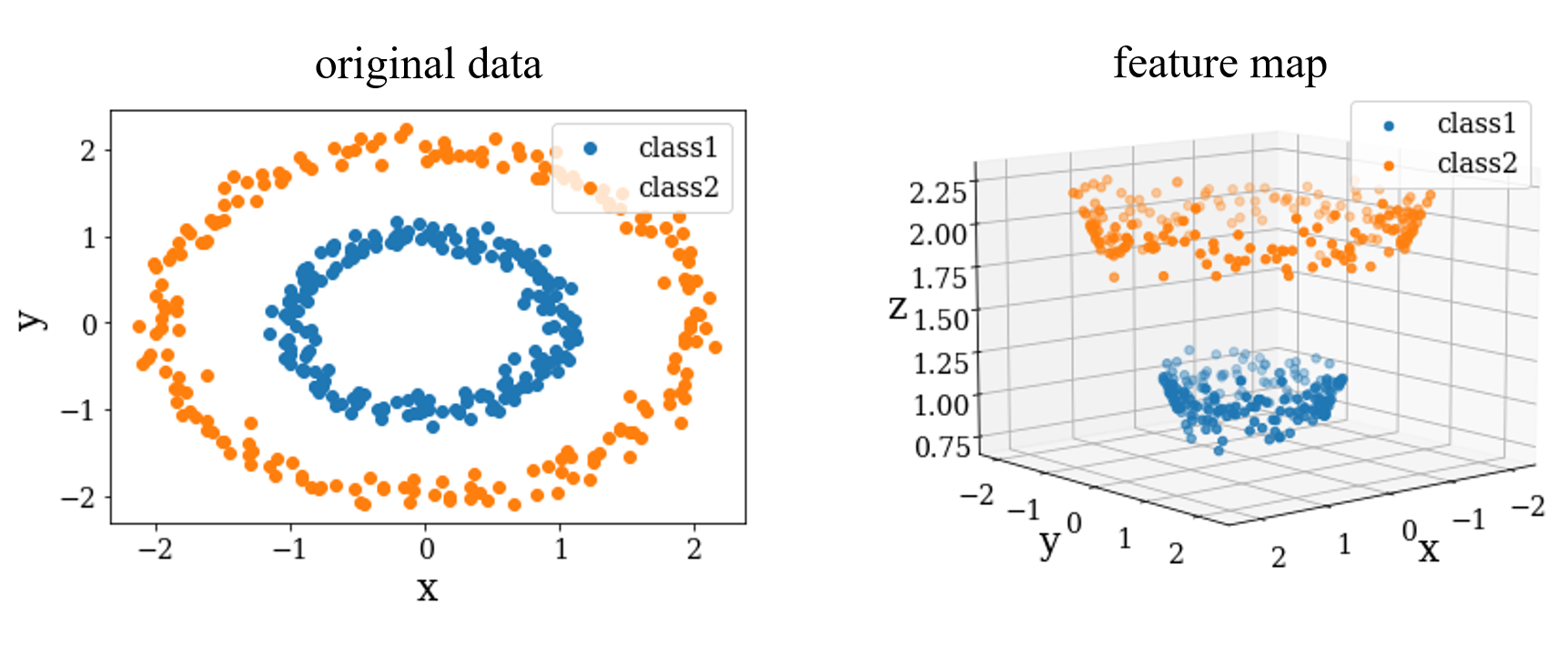
Figure 1: Mapping to feature space by the kernel function. The left panel represents a two-dimensional data set that is not linearly separable, and the right panel in Figure 1 shows an example of how it can be transformed into a three-dimensional data set with the addition of $z=\sqrt{x^{2}+y^{2}}$ dimension to make it linearly separable.

Random Fourier feature

In general, the kernel function is computed for a combination of two data points $\bm{x}$ and $\bm{x^{\prime}}$, consequently its computational complexity is $O(N^{2})$ for N number of data points. To reduce this computational complexity, we explicitly define the feature map $\varphi$ and approximate the kernel as $k(\bm{x},\bm{x^{\prime}})\approx\varphi(\bm{x})\varphi(\bm{x^{\prime}})$. With this procedure, if the dimension of $\varphi(\bm{x})$ is $S$, its computational complexity can be reduced to $O(NS)$[33]. In this method, we focus on the shift-invariant kernel functions $k(\bm{x},\bm{x^{\prime}})=k(\bm{x}-\bm{x^{\prime}})$ among kernel functions. The shift-invariant kernel is expressed as follows, by using the expected value of the spectral distribution from Bochner’s theorem.

$$k(\bm{x}-\bm{x^{\prime}})=\int_{\mathbb{R}_{d}}e^{i\bm{\omega}(\bm{x}-\bm{x^{\prime}})}dp(\bm{\omega})=E_{\bm{\omega}\sim p(\bm{\omega})}[e^{i{\bf\omega}(\bm{x}-\bm{x^{\prime}})}],$$ (1)

where $\omega$ is a random value obtained from the spectral distribution $p(\bm{\omega})$. By using a finite set $\{\bm{\omega}\}$, a low-variance approximation of the above equation can be obtained[34].

$$k(\bm{x}-\bm{x^{\prime}})=E_{\bm{\omega}\sim p(\bm{\omega})}[e^{i\bm{\omega}(\bm{x}-\bm{x^{\prime}}))}]\approx\frac{1}{S}\sum_{s}e^{i\bm{\omega}_{s}(\bm{x}-\bm{x^{\prime}})}.$$ (2)

Furthermore, since the kernel function is used as a real-value function, only the real-value part of the above equation is employed. Thus,

$$\left[\frac{1}{S}\sum_{s}e^{i\bm{\omega}_{s}(\bm{x}-\bm{x^{\prime}})}\right]_{\mathbb{R}}=\frac{1}{S}\sum_{s}\cos\bm{\omega}_{s}(\bm{x}-\bm{x^{\prime}})=\varphi(\bm{x})\varphi(\bm{x^{\prime}}).$$ (3)

The function $\varphi(\bm{x})$ is defined as follows.

$$\varphi(\bm{x})=\frac{1}{\sqrt{S}}(\cos\bm{\omega}_{1}\bm{x},\cos\bm{\omega}_{2}\bm{x},\cdots,\cos\bm{\omega}_{s}\bm{x},\sin\bm{\omega}_{1}\bm{x},\sin\bm{\omega}_{2}\bm{x},\cdots,\cos\bm{\omega}_{s}\bm{x}).$$ (4)

As a result, the shift-invariant kernel is represented by the feature map $\varphi$ that can be derived by using a random finite set $\{\omega\}$, and its computational complexity can be set to $O(NS)$.

Kernel Learning

A kernel function can be defined arbitrarily as far as expressed in the inner product. On the other hand, there is no systematic approach to selecting the best kernel function that fits the data. Instead of heuristically selecting the kernel function, there is a method called multiple Kernel Learning, which combines existing kernels to obtain a better kernel function that fits the data[31]. Recently, there is also a method called Implicit Kernel Learning (IKL), which learns a kernel function by learning the spectral distribution of the kernel function[29]. Implicit Kernel Learning is a new method that models spectral distributions by learning the sampling process. Thus, kernel selection can be replaced by optimized learning of the spectral distribution.

$$\arg\max_{k\in K}\sum_{i=1}E_{\bm{x}\sim p_{i},\bm{x^{\prime}}\sim q_{i}}[F_{i}(\bm{x},\bm{x^{\prime}})k(\bm{x},\bm{x^{\prime}})]=\arg\max_{k\in K}\sum_{i=1}E_{\bm{x}\sim p_{i},\bm{x^{\prime}}\sim q_{i}}\left[F_{i}(\bm{x},\bm{x^{\prime}})E_{\bm{\omega}\sim p(\bm{\omega})}[e^{i\bm{\omega}(\bm{x}-\bm{x^{\prime}})}]\right],$$ (5)

where function $F_{i}(\bm{x},\bm{x^{\prime}})$ represents the learning task-specific objective function[29]. To perform the classification task in this study, we set $F_{i}(\bm{x},\bm{x^{\prime}})=yy^{\prime}$, where $y$ and $y^{\prime}$ are the labels $\{+1,-1\}$ of the data $\bm{x}$ and $\bm{x^{\prime}}$, respectively. This corresponds to treating $\bm{x},\bm{x^{\prime}}$ as similar data in the feature space by maximizing the above equation when $y,y^{\prime}$ have the same label, and treating $\bm{x},\bm{x^{\prime}}$ as different data in the feature space by minimizing the above equation when $y,y^{\prime}$ have different labels. Our method consists of two steps. In step 1, kernel functions are learned, and in step 2, classification learning is performed using the learned kernel functions.

Quantum annealing

Quantum annealing is an algorithm that searches for the ground state of the Ising model shown below by using quantum effects[1].

$$H_{\text{ising}}=\sum_{i}h_{i}{\hat{\sigma}}_{z}^{i}+\sum_{ij(>i)}J_{ij}{\hat{\sigma}}_{z}^{i}{\hat{\sigma}}_{z}^{j},$$ (6)

where $\hat{\sigma}_{z}^{i}$ is the Pauli matrix on the i-th qubit, $h_{i}$ and $J_{ij}$ are the bias on each qubit and coupling strength between each pair of qubits, respectively. In actual quantum annealing machines, the following Hamiltonian, which adds $\sum_{i}{\hat{\sigma}}_{x}^{i}$ to the Ising model, is used.

$$H=\frac{A(s)}{2}\sum_{i}{\hat{\sigma}}_{x}^{i}+\frac{B(s)}{2}\left(\sum_{i}h_{i}{\hat{\sigma}}_{z}^{i}+\sum_{ij(>i)}J_{ij}{\hat{\sigma}}_{z}^{i}{\hat{\sigma}}_{z}^{j}\right),$$ (7)

where $\hat{\sigma}_{x}^{i}$ is the Pauli matrix on the i-th qubit, and $s$ is called the annealing rate. $A(s)$ and $B(s)$ are known as annealing functions. At the initial state of quantum annealing, i.e., when $s=0$, the annealing function is $A(s)\gg B(s)$, and the qubits are in a global superposition state that is the ground state of $\sum_{i}{\hat{\sigma}}_{x}^{i}$. Then, as $s$ is increased from $0$ to $1$, the ground state of the Hamiltonian changes. Finally, when $s=1$, $A(s)\ll B(s)$, and the qubits converge to a single classical state. At this point, the state $\hat{\sigma}_{z}^{i}$ of the Ising model is obtained. The output of an actual quantum annealing machine is known to follow the Gibbs-Boltzmann distribution due to thermal effects and residual magnetic fields due to the freezing effect.

Kernel Learning with RBM

In this study, we use the multi-layer RBM as shown in the left-hand side of Figure 2 for $\bm{\omega}$ sampling. The Gibbs-Boltzmann distribution is used as the spectral distribution.

$$P(\bm{v},\bm{h}|\bm{b},\bm{c},w)=\frac{e^{-E(\bm{v},\bm{h}|\bm{b},\bm{c},w)}}{Z(\bm{b},\bm{c},w)}$$ (8)

$$E(\bm{v},\bm{h}|\bm{b},\bm{c},w)=-\sum_{i}{b_{i}v_{i}}-\sum_{j}{c_{j}h_{j}}-\sum_{ij}{v_{i}w_{ij}h_{j}},$$ (9)

where $Z$ represents the partition function, $b_{i},c_{j}$ are bias terms, and $w_{jk}$ is the coupling strength between variables $v_{i}$ and $h_{j}$. After sampling from the Gibbs-Boltzmann distribution, a Gaussian-Bernoulli type RBM is used to transform the discrete variable $\bm{v}$ into a continuous variable $\bm{\omega}$.

$$P(\bm{\omega}|\bm{a},u,\bm{v},\bm{\sigma})=\frac{e^{-E(\bm{\omega}|\bm{a},u,\bm{v},\bm{\sigma})}}{Z(\bm{\omega}|\bm{a},u,\bm{v},\bm{\sigma})}=\frac{1}{\sqrt{2\pi}\bm{\sigma}}e^{-\frac{\left(\bm{\omega}-(\bm{a}+U\bm{v})\right)^{2}}{2\bm{\sigma}^{2}}}$$ (10)

$$E(\bm{\omega}|\bm{a},\bm{v},u,\bm{\sigma})=\sum_{i}\frac{(\omega_{i}-a_{i})^{2}}{2\sigma_{i}^{2}}-\sum_{ij}{\frac{\omega_{i}}{\sigma_{i}^{2}}\ u_{ij}v_{i}},$$ (11)

where $a_{i}$ is the bias and $u_{ij}$ is the coupling strength between variables $\omega_{i}$ and $v_{j}$, respectively. $\sigma_{i}$ is the standard deviation with respect to variable $\omega_{i}$. Specifically, the number of nodes in the RBM was set to $\{N_{\bm{\omega}},N_{\bm{v}},N_{\bm{h}}\}=\{10,4,4\}$, as shown in the left-hand side of Figure 2. D-Wave Advantage is used for sampling the visible layers $\{v_{1},v_{2},v_{3},v_{4}\}$ and the hidden layers $\{h_{1},h_{2},h_{3},h_{4}\}$. The D-Wave Advantage has a graph structure where the qubits are not fully connected, as shown on the right-hand side of Figure 2. Since there are subgraphs in the graph that can form a bipartite graph with 8 qubits, the visible and hidden layers were embedded in that bipartite graph. When performing quantum annealing, the Hamiltonian was constructed with $\{h_{1},\cdots,h_{8}\}=\{b_{1},\cdots,b_{4},c_{1},\cdots,c_{4}\}$ and $\{J_{14},\cdots,J_{48}\}=\{w_{11},\cdots,w_{44}\}$. As a result of the sampling, $(\hat{\sigma}_{z}^{1},\cdots,\hat{\sigma}_{z}^{8})=\{v_{1},\cdots,v_{4},h_{1},\cdots,h_{4}\}$ are obtained.

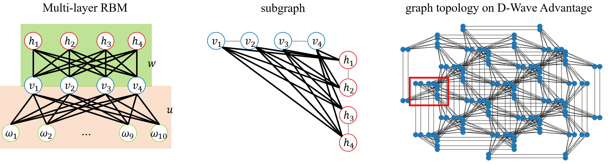
Figure 2: Boltzmann machine and minor embedding. The figure on the left-hand side is a multi-layer RBM. The number of nodes is $\{N_{\bm{\omega}},N_{\bm{v}},N_{\bm{h}}\}=\{10,4,4\}$.$w$ and $u$ are matrices of coupling strength between $\bm{v}$, $\bm{h}$ and $\bm{\omega}$, $\bm{v}$ respectively. right-hand side graph topology on D-Wave Advantage and subgraph. The black line represents the interaction.

Next, we discuss the RBM parameter updates. In this experiment, the loss function is defined in the section Kernel Learning;

$$L=\frac{1}{N^{2}}\sum_{ij}{y_{i}y_{j}E_{\bm{\omega}}[e^{i{\bf\omega}(\bm{x}_{i}-\bm{x}_{j})}]}.$$ (12)

The gradient of the loss function is expressed below using the Boltzmann machine parameter $\theta$.

$$\frac{\partial L}{\partial\theta}=\frac{1}{N^{2}}\sum_{ij}{y_{i}y_{j}\frac{\partial}{\partial\theta}E_{\bm{\omega}}[e^{i{\bf\omega}(\bm{x}_{i}-\bm{x}_{j})}]}.$$ (13)

Here, approximating the expectation calculation by sampling $\{\omega_{1},\omega_{2},\cdots,\omega_{S}\}$, the gradient can be calculated as follows,

$$\frac{\partial L}{\partial\theta}=\frac{1}{N^{2}}\sum_{ij}{y_{i}y_{j}\frac{\partial}{\partial\theta}E_{\bm{\omega}}[e^{i{\bf\omega}(\bm{x}_{i}-\bm{x}_{j})}]}=\frac{1}{N^{2}}\sum_{ij}{\sum_{s}{y_{i}y_{j}e^{i{\bf\omega_{s}}(\bm{x}_{i}-\bm{x}_{j})}\frac{\partial}{\partial\theta}P(\omega_{s}|\theta)}}.$$ (14)

In this study of RBM learning, the probability distribution is expressed as follows,

$$P(\bm{\omega}|\bm{a},u,\bm{v},\bm{\sigma})P(\bm{v},\bm{h}|\bm{b},\bm{c},w)=\frac{e^{-E(\bm{\omega},\bm{v},\bm{h}|\bm{a},\bm{b},\bm{c},w,u,\bm{\sigma})}}{Z(\bm{a},\bm{b},\bm{c},w,u,\bm{\sigma})}\equiv P(\bm{\omega},\bm{v},\bm{h}|\bm{a},\bm{b},\bm{c},w,u,\bm{\sigma})$$ (15)

$$E(\bm{\omega},\bm{v},\bm{h}|\bm{a},\bm{b},\bm{c},w,u,\bm{\sigma})=\sum_{i}\frac{(\omega_{i}-a_{i})^{2}}{2\sigma_{i}^{2}}-\sum_{j}{b_{j}v_{i}}-\sum_{ij}{\frac{\omega_{i}}{\sigma_{i}^{2}}u_{ij}v_{i}}-\sum_{k}{c_{k}h_{k}}-\sum_{jk}{v_{j}w_{jk}h_{k}}.$$ (16)

From $\sigma_{i}^{2}\geq 0$, we parametrize $\sigma_{i}^{2}$ as $e^{z_{i}}$ and write $\{\bm{a},\bm{b},\bm{c},w,u,\bm{\sigma}\}=\theta$.
The gradient $\frac{\partial}{\partial\theta}P(\bm{\omega},\bm{v},\bm{h}|\theta)=\frac{\partial}{\partial\theta}e^{-E(\bm{\omega},\bm{v},\bm{h}|\theta)}/Z(\theta)$ of the Gibbs-Boltzmann distribution can then be calculated as follows,

$$\frac{\partial}{\partial\theta}\frac{e^{-E(\bm{\omega},\bm{v},\bm{h}|\theta)}}{Z(\theta)}=\left\{-\frac{\partial}{\partial\theta}E(\bm{\omega},\bm{v},\bm{h}|\theta)-\frac{1}{Z(\theta)}\frac{\partial}{\partial\theta}Z(\theta)\right\}\frac{e^{-E(\bm{\omega},\bm{v},\bm{h}|\theta)}}{Z(\theta)}=\left\{-\frac{\partial}{\partial\theta}E(\bm{\omega},\bm{v},\bm{h}|\theta)-\frac{1}{Z(\theta)}\frac{\partial}{\partial\theta}Z(\theta)\right\}p(\bm{\omega}|\theta).$$ (17)

Thus, the gradient of the loss function is as follows. The calculation of each parameter is described in the appendix.

$$\frac{\partial L}{\partial\theta}=\frac{1}{N^{2}}\sum_{ij}{\frac{1}{S}\sum_{s}{y_{i}y_{j}e^{i\bm{\omega}_{s}(\bm{x}_{i}-\bm{x}_{j})}}}\left\{-\frac{\partial}{\partial\theta}E(\bm{\omega},\bm{v},\bm{h}|\theta)-\frac{1}{Z(\theta)}\frac{\partial}{\partial\theta}Z(\theta)\right\}_{\bm{\omega}_{s}}.$$ (18)

Similarly to equation (3), the gradient of the loss function can also be separate with respect to indices $i$ and $j$.

$$\frac{\partial L}{\partial\theta}=\frac{1}{N^{2}}\sum_{ij}{\frac{1}{S}\sum_{s}{y_{i}y_{j}e^{i\bm{\omega}_{s}(\bm{x}_{i}-\bm{x}_{j})}}}\left\{-\frac{\partial}{\partial\theta}E(\bm{\omega},\bm{v},\bm{h}|\theta)-\frac{1}{Z(\theta)}\frac{\partial}{\partial\theta}Z(\theta)\right\}_{\bm{\omega}_{s}}=\frac{1}{N^{2}}\sum_{i}{y_{i}\psi(\bm{x}_{i})\sum_{j}{y_{j}\varphi(\bm{x}_{j})}},$$ (19)

where $\psi(\bm{x})$ is defined;

$$\psi(\bm{x})=\frac{1}{\sqrt{S}}\Biggl{(}\left\{-\frac{\partial}{\partial\theta}E(\bm{\omega},\bm{v},\bm{h}|\theta)-\frac{1}{Z(\theta)}\frac{\partial}{\partial\theta}Z(\theta)\right\}_{\bm{\omega}_{1}}\cos{\bm{\omega}_{1}\bm{x}},\cdots,\left\{-\frac{\partial}{\partial\theta}E(\bm{\omega},\bm{v},\bm{h}|\theta)-\frac{1}{Z(\theta)}\frac{\partial}{\partial\theta}Z(\theta)\right\}_{\bm{\omega}_{S}}\cos{\bm{\omega}_{S}\bm{x}},\\ \left\{-\frac{\partial}{\partial\theta}E(\bm{\omega},\bm{v},\bm{h}|\theta)-\frac{1}{Z(\theta)}\frac{\partial}{\partial\theta}Z(\theta)\right\}_{\bm{\omega}_{1}}\sin{\bm{\omega}_{1}\bm{x}},\cdots,\left\{-\frac{\partial}{\partial\theta}E(\bm{\omega},\bm{v},\bm{h}|\theta)-\frac{1}{Z(\theta)}\frac{\partial}{\partial\theta}Z(\theta)\right\}_{\bm{\omega}_{S}}\sin{\bm{\omega}_{S}\bm{x}}\Biggl{)}.$$ (20)

In step 2, classification learning is performed using the learned kernel function. The classifier uses a kernel perceptron, which is a kernelized perceptron. The given data points are transformed with the feature function $\phi(\bm{x})$ acquired by kernel learning, and the inner product with the weight matrix $\sum_{i}^{N}{\bm{\alpha}_{i}y_{i}\phi(x_{i})}$ is calculated. Initially, $\bm{\alpha}=(\alpha_{1},\alpha_{2},\cdots,\alpha_{N})$ is set as an all-zero vector, and the value is updated when the output is different from the label. This operation is repeated for the number of iterations.

$$f(\bm{x})=sign\left(\sum_{i}^{N}\alpha_{i}y_{i}\phi(\bm{x}_{i})\phi(\bm{x})\right)=sign\left(\sum_{i}^{N}\alpha_{i}y_{i}k(\bm{x}_{i},\bm{x})\right).$$ (21)

If $f(\bm{x})$ is different from the label $y$, the parameter is updated by adding the learning rate to $\alpha$ and using the new $\alpha$ as the new value. To prevent over-fitting, regularization is applied so that the size of $\alpha$ does not exceed $0.5$.

Results

Fashion MNIST, which is used in the field of deep learning and machine learning for image recognition tasks, was used as the dataset for verification. In the experiment, 1000 images of two specific classes were taken from each of the two classes, and 784 dimensions were compressed into 10 dimensions by principal component analysis (PCA) and used. Because of the cost involved in using a quantum annealer, 500 RBMs were embedded in subgraphs on D-Wave Advantage in Figure 2 at the same time. Then we get 1000 samples in total. Next, we show experimental results. Figure 3 shows the loss of kernel learning. As a comparison, this experiment uses a Gaussian distribution for the spectral distribution and shows the Loss when the loss function is minimized using the parameter optimization tool, Optuna[35]. The figure shows that kernel learning was more efficient in searching for the minimum loss function for all data sets.

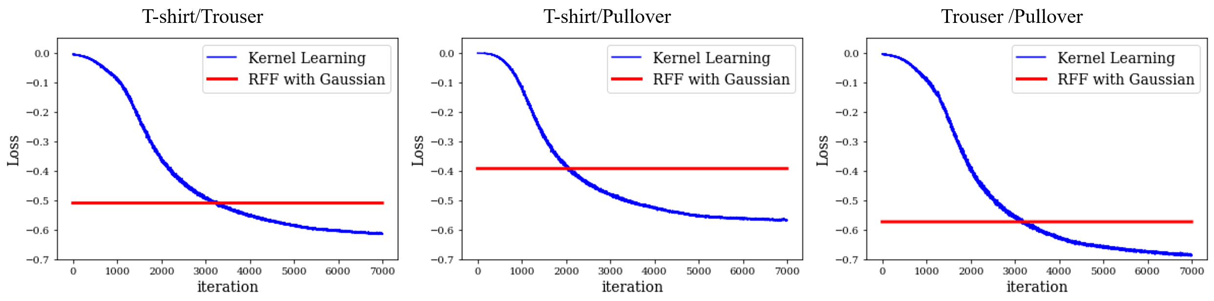
Figure 3: Loss of kernel learning. The blue curve represents the value of the loss function by kernel learning, and the red curve represents the loss when the spectral distribution is Gaussian and the loss function is minimized using Optuna. Classification learning of T-shirt/Trouser, T-shirt/Pullover, and Trouser/Pullover, respectively.

Figure 4 also shows the kernel matrices before and after kernel learning. It can be confirmed that kernel learning enables classification, as the kernel component $k(\bm{x}_{i},\bm{x}_{j})$ is larger for data with the same labels, and the kernel component $k(\bm{x}_{i},\bm{x}_{j})$ is smaller for data with different labels.

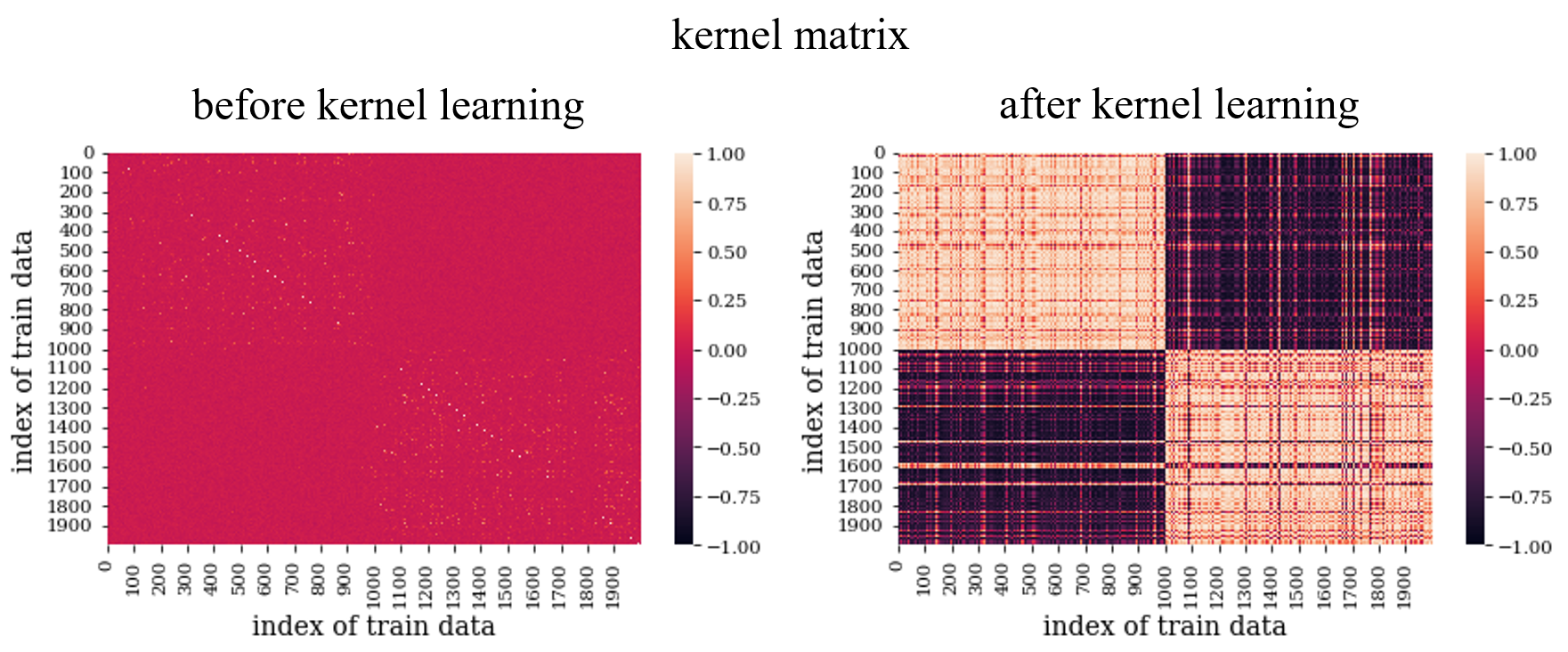
Figure 4: kernel matrix before and after kernel learning. The left panel represents the kernel matrix before kernel training, and the right panel represents the kernel matrix after kernel training. The vertical and horizontal axes are the indices of the data, respectively.

Figure 5 shows the sampling of $\bm{\omega}$ for RFF using kernel learning and Gaussian distribution when training the T-shirt/Trouser dataset. It can be seen that when using the Gaussian distribution, the distribution of $\bm{\omega}$ is Gaussian, whereas when using kernel learning, a distribution with two peaks is generated. Therefore, it is possible to sample $\bm{\omega}$ with a higher degree of freedom than when using a Gaussian distribution for the spectral distribution.

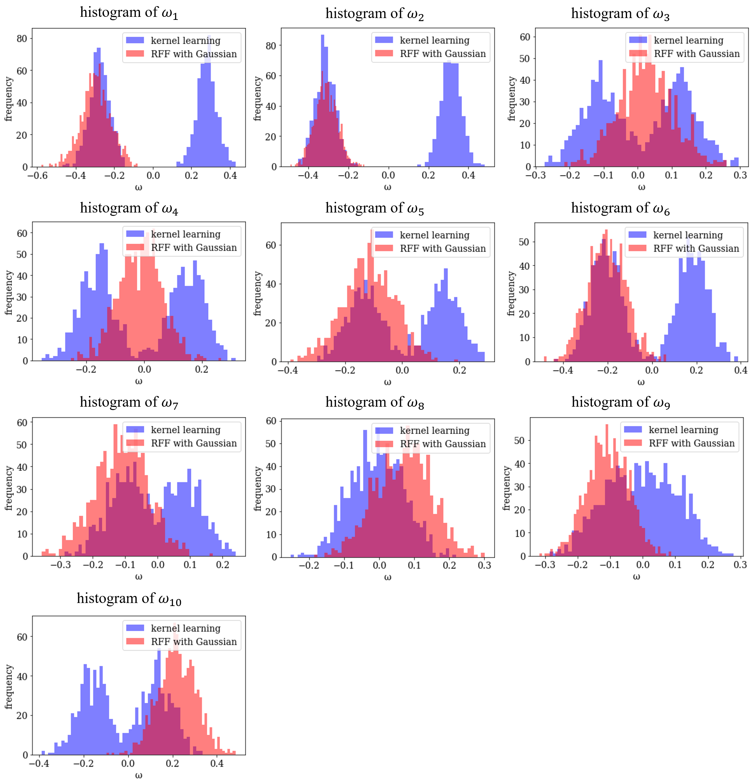
Figure 5: $\bm{\omega}$ sampling in T-shirt/Trouser dataset. The distribution of each component of $\bm{\omega}$ after learning T-shirt/Trouser dataset. The vertical axis represents the frequency and the horizontal axis represents the value of $\bm{\omega}$. The blue bar represents $\bm{\omega}$ sampled by kernel learning, and the red bar represents $\bm{\omega}$ sampled by RFF.

Table 1 shows the prediction accuracy for each dataset. As can be seen from the table, the classification accuracy was highest after kernel training.

T-shirt/Trouser	Before Kernel Learning	After Kernel Learning	RFF with Gaussian
Train Data	1.000	0.990	0.985
Test Data	0.932	0.989	0.982

T-shirt/Pullover	Before Kernel Learning	After Kernel Learning	RFF with Gaussian
Train Data	1.000	0.967	0.975
Test Data	0.824	0.957	0.956

Trouser/Pullover	Before Kernel Learning	After Kernel Learning	RFF with Gaussian
Train Data	1.000	0.994	0.993
Test Data	0.971	0.988	0.986

Table 1: Learning Accuracy. List of RFF prediction accuracies before kernel training, after kernel training, and using Gaussian distributions for each dataset. The bolded text indicates the highest prediction accuracy for each dataset.

Discussion and Conclusion

We show a kernel function using the Gibbs-Boltzmann distribution as the spectral distribution, and it is shown that a kernel function that suits to the data set is obtained by kernel learning using the Boltzmann machine. We confirmed that the prediction accuracy is comparable to that of the method using the Gaussian distribution.
We also showed that it is possible to create a distribution of $\bm{\omega}$ with more degrees of freedom than the method using a Gaussian distribution.
From the results, we were able to adopt a multi-layer RBM as a model for kernel learning and to propose an application that uses a quantum annealer for learning RBMs, which can be used as a fast sampling machine.
On the other hand, the relevance of the number of nodes in the hidden layer of the Boltzmann machine to the distribution of $\bm{\omega}$ and the prediction accuracy needs to be investigated. In addition, it is unclear how to take advantage of the quantum nature of quantum computers.
We will continue to explore applications where quantum annealers can be used as sampling machines.

Appendix

Appendix A The gradient of kernel learning loss function

The gradient of Gibbs-Boltzmann distribution and kernel learning loss function can be calculated as follows,

$$\frac{\partial}{\partial\theta}\frac{e^{-E(\bm{\omega},\bm{v},\bm{h}|\theta)}}{Z(\theta)}=\left\{-\frac{\partial}{\partial\theta}E(\bm{\omega},\bm{v},\bm{h}|\theta)-\frac{1}{Z(\theta)}\frac{\partial}{\partial\theta}Z(\theta)\right\}\frac{e^{-E(\bm{\omega},\bm{v},\bm{h}|\theta)}}{Z(\theta)}=\left\{-\frac{\partial}{\partial\theta}E(\bm{\omega},\bm{v},\bm{h}|\theta)-\frac{1}{Z(\theta)}\frac{\partial}{\partial\theta}Z(\theta)\right\}p(\bm{\omega}|\theta).$$ (A1)

$$\frac{\partial L}{\partial\theta}=\frac{1}{N^{2}}\sum_{ij}{\frac{1}{S}\sum_{s}{y_{i}y_{j}e^{i\bm{\omega}_{s}(\bm{x}_{i}-\bm{x}_{j})}}}\left\{-\frac{\partial}{\partial\theta}E(\bm{\omega},\bm{v},\bm{h}|\theta)-\frac{1}{Z(\theta)}\frac{\partial}{\partial\theta}Z(\theta)\right\}_{\bm{\omega}_{s}}.$$ (A2)

Each parameter is calculated as follows,

$$\frac{\partial L}{\partial a_{i}}=\frac{1}{N^{2}}\sum_{ij}{\frac{1}{S}\sum_{s}{y_{i}y_{j}e^{i\bm{\omega}_{s}(\bm{x}_{i}-\bm{x}_{j})}}}\left\{\frac{(\omega_{i}-a_{i})}{e^{z_{i}}}-\frac{1}{Z(\theta)}\frac{\partial}{\partial a_{i}}Z(\theta)\right\}_{\bm{\omega}_{s}}$$ (A3)

$$\frac{\partial L}{\partial b_{j}}=\frac{1}{N^{2}}\sum_{ij}{\frac{1}{S}\sum_{s}{y_{i}y_{j}e^{i\bm{\omega}_{s}(\bm{x}_{i}-\bm{x}_{j})}}}\left\{v_{j}-\frac{1}{Z(\theta)}\frac{\partial}{\partial b_{j}}Z(\theta)\right\}_{\bm{\omega}_{s}}$$ (A4)

$$\frac{\partial L}{\partial c_{k}}=\frac{1}{N^{2}}\sum_{ij}{\frac{1}{S}\sum_{s}{y_{i}y_{j}e^{i\bm{\omega}_{s}(\bm{x}_{i}-\bm{x}_{j})}}}\left\{h_{k}-\frac{1}{Z(\theta)}\frac{\partial}{\partial c_{k}}Z(\theta)\right\}_{\bm{\omega}_{s}}$$ (A5)

$$\frac{\partial L}{\partial u_{ij}}=\frac{1}{N^{2}}\sum_{ij}{\frac{1}{S}\sum_{s}{y_{i}y_{j}e^{i\bm{\omega}_{s}(\bm{x}_{i}-\bm{x}_{j})}}}\left\{\frac{\omega_{i}}{e^{z_{i}}}v_{j}-\frac{1}{Z(\theta)}\frac{\partial}{\partial u_{ij}}Z(\theta)\right\}_{\bm{\omega}_{s}}$$ (A6)

$$\frac{\partial L}{\partial w_{jk}}=\frac{1}{N^{2}}\sum_{ij}{\frac{1}{S}\sum_{s}{y_{i}y_{j}e^{i\bm{\omega}_{s}(\bm{x}_{i}-\bm{x}_{j})}}}\left\{v_{j}h_{k}-\frac{1}{Z(\theta)}\frac{\partial}{\partial w_{jk}}Z(\theta)\right\}_{\bm{\omega}_{s}}$$ (A7)

$$\frac{\partial L}{\partial z_{i}}=\frac{1}{N^{2}}\sum_{ij}{\frac{1}{S}\sum_{s}{y_{i}y_{j}e^{i\bm{\omega}_{s}(\bm{x}_{i}-\bm{x}_{j})}}}\left\{-\frac{(\omega_{i}-a_{i})^{2}}{2e^{z_{i}}}+\frac{\omega_{i}}{e^{z_{i}}}u_{ij}v_{j}-\frac{1}{Z(\theta)}\frac{\partial}{\partial z_{i}}Z(\theta)\right\}_{\bm{\omega}_{s}}.$$ (A8)

Here, $\bm{v},\bm{h}$ are sampled in the experiment as well as $\bm{\omega}$. In oter words, we obtain samples $\left\{(\bm{\omega}_{1},\bm{v}_{1},\bm{h}_{1}),(\bm{\omega}_{2},\bm{v}_{2},\bm{h}_{2}),\cdots,(\bm{\omega}_{S},\bm{v}_{S},\bm{h}_{S})\right\}$. Therefore, when calculating each parameter, we use $\bm{v}$ and $\bm{h}$ associated with $\bm{\omega}$.

References

- [1] Ray, P., Chakrabarti, B. K. & Chakrabarti, A. Sherrington-kirkpatrick model in a transverse field: Absence of replica symmetry breaking due to quantum fluctuations (1989).
- [2] Kadowaki, T. & Nishimori, H. Quantum annealing in the transverse ising model. \JournalTitlePhys. Rev. E 58, 5355–5363, DOI: 10.1103/PhysRevE.58.5355 (1998).
- [3] Yarkoni, S., Raponi, E., Bäck, T. & Schmitt, S. Quantum annealing for industry applications: introduction and review. \JournalTitleReports on Progress in Physics 85, DOI: 10.1088/1361-6633/ac8c54 (2022).
- [4] Rosenberg, G. et al. Solving the optimal trading trajectory problem using a quantum annealer. \JournalTitleIEEE Journal on Selected Topics in Signal Processing 10, 1053–1060, DOI: 10.1109/JSTSP.2016.2574703 (2016).
- [5] Venturelli, D. & Kondratyev, A. Reverse quantum annealing approach to portfolio optimization problems. \JournalTitleQuantum Machine Intelligence 1, 17–30, DOI: 10.1007/s42484-019-00001-w (2019).
- [6] Hernandez, M. & Aramon, M. Enhancing quantum annealing performance for the molecular similarity problem. \JournalTitleQuantum Information Processing 16, DOI: 10.1007/s11128-017-1586-y (2017).
- [7] Streif, M., Neukart, F. & Leib, M. Solving quantum chemistry problems with a d-wave quantum annealer. In Feld, S. & Linnhoff-Popien, C. (eds.) Quantum Technology and Optimization Problems, 111–122 (Springer International Publishing, Cham, 2019).
- [8] Venturelli, D., Marchand, D. J. J. & Rojo, G. Quantum annealing implementation of job-shop scheduling (2016). 1506.08479.
- [9] Ikeda, K., Nakamura, Y. & Humble, T. S. Application of quantum annealing to nurse scheduling problem. \JournalTitleScientific Reports 9, DOI: 10.1038/s41598-019-49172-3 (2019).
- [10] Yarkoni, S. et al. Multi-car paint shop optimization with quantum annealing (2021). 2109.07876.
- [11] Stollenwerk, T. et al. Quantum annealing applied to de-conflicting optimal trajectories for air traffic management. \JournalTitleIEEE Transactions on Intelligent Transportation Systems 21, 285–297, DOI: 10.1109/TITS.2019.2891235 (2020).
- [12] Inoue, D., Okada, A., Matsumori, T., Aihara, K. & Yoshida, H. Traffic signal optimization on a square lattice with quantum annealing. \JournalTitleScientific Reports 11, DOI: 10.1038/s41598-021-82740-0 (2021).
- [13] Neven, H., Denchev, V. S., Rose, G. & Macready, W. G. Training a large scale classifier with the quantum adiabatic algorithm. \JournalTitleCoRR abs/0912.0779 (2009). 0912.0779.
- [14] Macready, W. G. et al. Nips 2009 demonstration: Binary classification using hardware implementation of quantum annealing (2010).
- [15] Neukart, F., Dollen, D. V., Seidel, C. & Compostella, G. Quantum-enhanced reinforcement learning for finite-episode games with discrete state spaces. \JournalTitleFrontiers in Physics 5, 71, DOI: 10.3389/fphy.2017.00071 (2018).
- [16] Crawford, D., Levit, A., Ghadermarzy, N., Oberoi, J. S. & Ronagh, P. Reinforcement learning using quantum boltzmann machines (2019). 1612.05695.
- [17] Sato, T., Ohzeki, M. & Tanaka, K. Assessment of image generation by quantum annealer. \JournalTitleScientific Reports 11, DOI: 10.1038/s41598-021-92295-9 (2021).
- [18] Nishimura, N., Tanahashi, K., Suganuma, K., Miyama, M. J. & Ohzeki, M. Item listing optimization for e-commerce websites based on diversity. \JournalTitleFrontiers in Computer Science 1, DOI: 10.3389/fcomp.2019.00002 (2019).
- [19] Ohzeki, M., Miki, A., Miyama, M. J. & Terabe, M. Control of automated guided vehicles without collision by quantum annealer and digital devices. \JournalTitleFrontiers in Computer Science 1, DOI: 10.3389/fcomp.2019.00009 (2019).
- [20] Haba, R., Ohzeki, M. & Tanaka, K. Travel time optimization on multi-agv routing by reverse annealing. \JournalTitleScientific Reports 12, 17753, DOI: 10.1038/s41598-022-22704-0 (2022).
- [21] Ide, N., Asayama, T., Ueno, H. & Ohzeki, M. Maximum-likelihood channel decoding with quantum annealing machine (2020). 2007.08689.
- [22] Arai, S., Ohzeki, M. & Tanaka, K. Mean field analysis of reverse annealing for code-division multiple-access multiuser detection. \JournalTitlePhys. Rev. Res. 3, 033006, DOI: 10.1103/PhysRevResearch.3.033006 (2021).
- [23] Adachi, S. H. & Henderson, M. P. Application of quantum annealing to training of deep neural networks (2015). 1510.06356.
- [24] Benedetti, M., Realpe-Gómez, J., Biswas, R. & Perdomo-Ortiz, A. Estimation of effective temperatures in quantum annealers for sampling applications: A case study with possible applications in deep learning. \JournalTitlePhysical Review A 94, 022308 (2016).
- [25] Arai, S., Ohzeki, M. & Tanaka, K. Teacher-student learning for a binary perceptron with quantum fluctuations. \JournalTitleJournal of the Physical Society of Japan 90, 074002, DOI: 10.7566/JPSJ.90.074002 (2021). https://doi.org/10.7566/JPSJ.90.074002.
- [26] Urushibata, M., Ohzeki, M. & Tanaka, K. Comparing the effects of boltzmann machines as associative memory in generative adversarial networks between classical and quantum samplings. \JournalTitleJournal of the Physical Society of Japan 91, 074008, DOI: 10.7566/JPSJ.91.074008 (2022). https://doi.org/10.7566/JPSJ.91.074008.
- [27] Salakhutdinov, R., Mnih, A. & Hinton, G. Restricted boltzmann machines for collaborative filtering.
- [28] Larochelle, H. & Bengio, Y. Classification using discriminative restricted boltzmann machines. 536–543, DOI: 10.1145/1390156.1390224 (Association for Computing Machinery, 2008).
- [29] Li, C.-L., Chang, W.-C., Mroueh, Y., Yang, Y. & Póczos, B. Implicit kernel learning (2019).
- [30] Mairal, J. End-to-end kernel learning with supervised convolutional kernel networks. \JournalTitleCoRR abs/1605.06265 (2016). 1605.06265.
- [31] Gönen, M. & Alpaydın, E. Multiple kernel learning algorithms (2011).
- [32] Karal, O. Performance comparison of different kernel functions in svm for different k value in k-fold cross-validation. DOI: 10.1109/ASYU50717.2020.9259880 (Institute of Electrical and Electronics Engineers Inc., 2020).
- [33] Liu, F., Huang, X., Chen, Y. & Suykens, J. A. K. Random features for kernel approximation: A survey on algorithms, theory, and beyond. \JournalTitleIEEE Transactions on Pattern Analysis and Machine Intelligence 44, 7128–7148, DOI: 10.1109/TPAMI.2021.3097011 (2022).
- [34] Rahimi, A. & Recht, B. Random features for large-scale kernel machines.
- [35] Akiba, T., Sano, S., Yanase, T., Ohta, T. & Koyama, M. Optuna: A next-generation hyperparameter optimization framework. 2623–2631, DOI: 10.1145/3292500.3330701 (Association for Computing Machinery, 2019).
Acknowledgements
I would like to thank Ohzeki, M. and Oshiyama, H. for useful discussions.