The Liquid–Hexatic Transition for Soft Disks

Abstract

We study the liquid–hexatic transition of soft disks with massively parallel simulations and determine the equation of state as a function of system size. For systems with interactions decaying as the inverse $m$th power of the separation, the liquid–hexatic phase transition is continuous for $m=12$ and $m=8$, while it is of first order for $m=24$. The critical power $m$ for the transition between continuous and first-order behavior is larger than previously reported. The continuous transition for $m=12$ implies that the two-dimensional Lennard-Jones model has a continuous liquid–hexatic transition at high temperatures. We also study the Weeks–Chandler–Andersen model and find a continuous transition at high temperatures, that is consistent with the soft-disk case for $m=12$. Pressure data as well as our implementation are available from an open-source repository.

I Introduction

Two-dimensional melting transitions are observed in multiple settings, including adatoms on metal surfaces [1, 2], colloids in confined geometries [3, 4, 5], skyrmions in magnetic materials [6, 7], and trapped electrons on the surface of ⁴He [8, 9]. Unlike their three-dimensional counterparts, that generically feature first-order liquid–crystal transitions, the nature of the phase transitions of two-dimensional particle systems depends on the details of interaction potentials and particle shapes [10, 11, 12]. In systems with short-range interactions, crystalline phases with long-range density correlations do not exist, since phonon excitations imply diverging fluctuations [13, 14, 15]. This mirrors the physics of two-dimensional $O(n)$ spin models, where phase transitions are absent for $n\geq 3$ [16]. For $n=2$ (the XY model) the low-temperature phase behavior is characterized by power-law spin–spin correlations and the presence of pairs of topological vortices. The Kosterlitz–Thouless phase transition between the two phases is now solidly established [17, 18, 19, 20].

Particle systems in two dimensions sustain two types of topological defect [17, 21, 22, 23], disclinations and dislocations. The KTHNY theory proposes that high-density solids melt into a liquid via two successive Kosterlitz–Thouless transitions, corresponding to the successive unbinding of dislocations, and then of disclinations. Between these two transitions, the intermediate hexatic phase short-range positional order and quasi-long-range orientational order. In an alternative scenario [24, 25], the solid melts directly into a liquid via a first-order transition due to the formation of grain boundaries. Most of the theories of two-dimensional melting worked within these two frameworks. For the special case of hard disks, however, decades of numerical studies going back to the dawn of Monte Carlo and molecular dynamics simulations [26, 27, 28], finally concluded [29] that nature chooses a first-order liquid–hexatic transition, and a continuous Kosterlitz–Thouless hexatic–solid transition. These results were confirmed in recent experiments [5], and they contradict the historic scenarios [29, 30].

The nature of the melting transition of soft disks with, for example, Lennard-Jones or (inverse) power-law potentials, may depend on model parameters, such as temperature and density. In Lennard-Jones systems, a number of conflicting transition scenarios have been reported [31, 32, 33, 34, 35, 12, 36]. The Lennard-Jones phase diagram can also be related to the case of power-law potentials of the form $U(r)={(\sigma/r)}^{m}$ [10, 34, 35], which interpolate between hard disks, $m=\infty$, and the soft potential with $m=3$, for which the KTHNY scenario is well-established [37].

The debate and controversies as to the order of the liquid–hexatic transition in two-dimensional soft-disk systems are due to remarkably strong finite-size effects. The determination of the order of the transition has largely relied on the presence or absence of a Mayer–Wood loop in the equation of state [38, 10, 35, 11]. The major difficulty is that the equation of state of finite systems may have a Mayer–Wood loop even when a transition is continuous. The loop then vanishes at a very large system size [39]. It is thus impossible to conclude on the nature of the transition with simulations on a single system size. Careful analysis of finite-size effects must be performed to reach a definitive conclusion.

In this paper, we revisit the liquid–hexatic transition for soft disks with large-scale parallel algorithms implemented on high-performance Graphics Processing Units (GPU). We generate high-precision Monte Carlo data on multiple system sizes up to $N=1024^{2}$ particles to better distinguish between the different scenarios. Following Ref. [40], we implement a massively parallel Metropolis algorithm, and determine equations of state to high precision for the power-law potentials with $m=8$, $12$, $24$, together with the Weeks–Chandler–Andersen (WCA) potential [41] at two different temperatures. We focus on the equation of state and carefully analyze the finite-size scaling of the free-energy barrier to determine the nature of the liquid–hexatic transition.

This paper is organized as follows. In Section II, we introduce the potentials that we study, together with the observables that we measure. We present our Monte Carlo results for inverse power-law models in Section III and for the WCA model in Section IV. Using the equation of state, we perform a detailed finite-size analysis and discuss the liquid–hexatic transition. In Section V, we summarize the results and present our conclusions as to the order of the liquid–hexatic transition.

II Models and method

We consider $N$ disks in a square periodic box of volume $V$, with two different interaction potentials. We are interested in the generic soft-disk model

$$U^{m}_{\infty}(r)/\epsilon={(r/\sigma)}^{-m}\quad(r>0),$$ (1)

where $\sigma$, a diameter, provides a length scale. Its phase behavior depends on the single parameter $\Gamma=\beta\epsilon{(\phi\sigma)}^{n/2}$, where $\beta$ is the inverse temperature and $\phi=N/V$ is the number density. Soft-disk systems with the infinite-range potential $U^{m}_{\infty}$ can be simulated with a computational complexity of $\mathcal{O}(1)$ per move (that is per event) using the cell-veto event-chain Monte Carlo algorithm [42]. Nevertheless, for computational convenience, a cutoff $r_{c}$ is often introduced in studies of long-range potentials [43, 44]. Simply restricting $U^{m}_{\infty}$ to separations smaller than a value $r_{c}$ complicates the calculation of virial pressures because of the discontinuity [45, 46] in the potential at $r=r_{c}$. These corrections in the pressure are absent in a continuous, shifted potential

$$U^{(m)}_{r_{c}}(r)/\epsilon=\begin{cases}\left(r/\sigma\right)^{-m}-\left(r_{c}/\sigma\right)^{-m}&(r<r_{c})\\ 0&(r>r_{c}).\end{cases}$$ (2)

This potential was studied in Ref. [42] with a cutoff $r_{c}/\sigma=1.8$, which we again use in this paper. The exact scaling in temperature and density, via $\Gamma$, does not strictly hold with a cutoff. However, we change only the number density and fix $\beta\epsilon=1$ for this family of potentials (see Section III for a discussion of the effects of the cutoff on the melting).

Our second model is the Weeks–Chandler–Anderson (WCA) model, that features a Lennard-Jones potential with a cutoff at its minimum shifted for continuity [41]:

$$U_{\text{WCA}}(r)/\epsilon=\begin{cases}4\left[\left(\frac{\sigma}{r}\right)^{12}-\left(\frac{\sigma}{r}\right)^{6}\right]+1,&\frac{r}{\sigma}<2^{1/6}\\ 0&\frac{r}{\sigma}>2^{1/6}.\end{cases}$$ (3)

The WCA potential is purely repulsive (the additional factor of $4$ in Eq. (3) compared to Eq. (2) comes from the usual definition of the Lennard-Jones model and is not taken into account in our discussions). We study it as a function of temperature and of number density. The system was studied previously at $\beta\epsilon=1$, where it has a first-order liquid–hexatic transition [47]. Because of their identical potential for small $r/\sigma$, the WCA model, the Lennard-Jones model, and the $m=12$ model have the same phase behavior at high temperatures and pressures.

We have implemented a massively parallel Metropolis algorithm on GPUs [40, 28]. Our implementation reaches $1.7\times 10^{13}$ individual Monte Carlo trials per hour for the power-law model with $m=12$ with $N=1024^{2}$ on an NVIDIA GeForce RTX 3090 GPU, which is more than $1000$ times faster than a sequential implementation. Our code thus requires some $4$ days for $1.6\times 10^{9}$ sweeps for $1024^{2}$ disks.

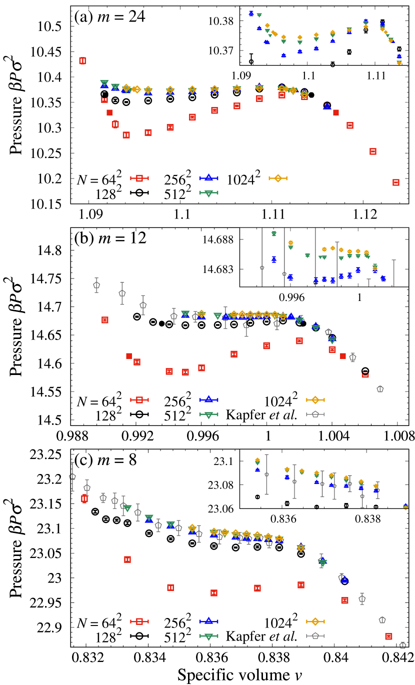
Figure 1: Equation of state of the power-law model of Eq. (2) for $N=64^{2}$, $128^{2}$, $256^{2}$, $512^{2}$, and $1024^{2}$. (a): For $m=24$, the loop is pronounced for all system sizes. (b): For $m=12$, the loop is tiny for $N=512^{2}$ and $1024^{2}$ and is expected to disappear for larger $N$. (c): $m=8$. The loop disappears for $N=256^{2}$, and the transition is clearly continuous. Data labeled as “Kapfer et al.” [10] is for $N\approx 255^{2}$. Filled symbols for each system size indicate the specific volumes of the liquid and hexatic phases, $v_{\text{liq}}$ and $v_{\text{hex}}$ ($v_{\text{liq}}>v_{\text{hex}}$).

We measure the equilibrium pressure from the virial

$$P=\frac{\phi}{\beta}-\frac{1}{2V}\left\langle\sum_{i>j}r_{ij}\frac{\partial U(r_{ij})}{\partial r_{ij}}\right\rangle,$$ (4)

where $r_{ij}=|\boldsymbol{r}_{i}-\boldsymbol{r}_{j}|$. For each system, we produce a single time series for the pressure, and estimate its correlations using the stationary bootstrap method [48, 49, 50, 51].

For hard disks as well as soft disks with large $m$, the equation of state has a ‘loop’, that is a non-monotonic variation of the pressure as a function of (inverse) density, close to the liquid–hexatic phase transition. The equation of state then becomes flat over a finite range of inverse density when $N\to\infty$. The existence of a loop in the equation of state of a finite system has been taken to indicate a first-order transition. However, the loop does not necessarily mean a first-order transition [38, 52] as we will show below. In order to determine the nature of the transition, it is essential to observe the finite-size dependence of the equation of state.

The Mayer–Wood loop in the equation of state (with the pressure being the derivative of the free energy with respect to the volume) results from a non-convex free energy as a function of the volume. In the presence of a first-order transition, that is, of coexistence of two phases of two distinct specific volumes, the free energy $F(v)$ as a function of specific volume $v={(\phi\sigma^{2})}^{-1}$ has two minima separated by a free-energy barrier $\Delta F$. Then the free-energy barrier scales as $\Delta F=O(L^{d-1})$ goes to $0$ and $f(v)=F(v)/N$ is convex when $N\to\infty$.

Nevertheless, $\Delta f$ can be nonzero and positive in finite systems [39]. The scaling of $\Delta f$ as a function of $N$ depends on the nature of the transition. For a first-order transition, the barrier comes from the surface free energy of a single compact droplet and thus $\Delta f=O(L^{d-1}/N)=O(L^{-1})$ in spatial dimension $d$, where $L$ is the size of the simulation box. The free-energy barrier $\Delta f$ should decay faster than $1/L$ for a continuous transition. We expect that the free energy becomes strictly convex and $\Delta f=0$ at large finite $N$ for a continuous liquid–hexatic transition. Practically, we numerically integrate the equation of state (as a function of the specific volume) to obtain the free energy and the specific volumes for the liquid and hexatic phases, $v_{\text{liq}}$ and $v_{\text{hex}}$ respectively, using a spline interpolation, and the bootstrap method to estimate the errors of $\Delta f$, $v_{\text{liq}}$, and $v_{\text{hex}}$.

III Power-law models

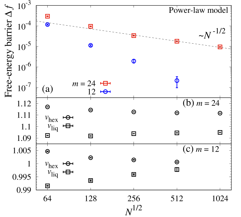
Figure 2: (a): Free-energy barrier $\Delta f$ as a function of $N^{1/2}$ for the power-law model of Eq. (2) with $m=24$ and $m=12$. For $m=24$, $\Delta f$ asymptotically scales as $N^{-1/2}$, indicating a first-order transition. For $m=12$, it decays faster, indicating a continuous transition. Specific volumes $v_{\text{liq}}$ and $v_{\text{hex}}$ as functions of $N^{1/2}$, for (b): $m=24$ and (c): $m=12$. For $m=24$, the specific volumes are well separated, consistent with the first-order transition. For $m=12$, on the other hand, $v_{\text{liq}}$ and $v_{\text{hex}}$ approach each other and eventually merge at $N=1024^{2}$, as seen in the monotonic equation of state Fig. 1 (b).

In this section, we study soft disks with potential $U^{(m)}_{r_{c}}$ for $m=24$, $12$, and $8$. The equilibrium pressure of the system is computed using Eq. (4). We show in Fig. 1 the equation of state, plotting the dimensionless pressure $\beta P\sigma^{2}$ as a function of specific volume $v={(\phi\sigma^{2})}^{-1}$.

For $m=24$, we observe a Mayer–Wood loop for small numbers of disks. While the loop amplitude decreases with $N$, it survives up to $N=1024^{2}$, Fig. 1 (a). A similar $N$ dependence of the equation of state has been observed in hard disks, equivalent to the $m\to\infty$ limit of the inverse power law [29, 30, 28]. We quantify the decay of the loop amplitude by the free-energy barrier $\Delta f$, Fig. 2 (a). $\Delta f$ decreases with increasing $N$. The barrier $\Delta f$ asymptotically scales as $\Delta f\sim N^{-1/2}\sim 1/L$ for large $N$, similarly to hard disks [29]. This is a strong indication of a first-order transition. The specific volumes of the liquid and hexatic phases $v_{\text{liq}}$ and $v_{\text{hex}}$ are well separated and do not merge, meaning the coexisting phase over a finite range of specific volume, see Fig. 2 (b).

The case $m=12$ also has a clear loop in the equation of state from $v\simeq 1.005$ to $0.992$ when $N=64^{2}$, Fig. 1 (b). In Ref. [10] it was concluded that the liquid–hexatic transition is first order. However, with increasing $N$, the loop shrinks too rapidly. Note that for $N=256^{2}$, our Monte Carlo results are consistent with Ref. [10] for $N=6.5\times 10^{4}\approx 255^{2}$. $\Delta f$ decays faster than the scaling $\Delta f\sim N^{-1/2}$ expected when the transition is of first order, and $v_{\text{liq}}$ and $v_{\text{hex}}$ merge at $N\simeq 1024^{2}$, see Fig. 2 (a) and (c). We thus conclude that for $m=12$ the liquid–hexatic transition is continuous, so that the hexatic melts into the liquid via a Kosterlitz–Thouless transition, following the conventional two-step scenario  [53, 21, 22, 23].

We observe similar finite-size effects for $m=8$ where the equation of state of the system for $N=128^{2}$ is almost monotonic; the continuous nature of the liquid–hexatic transition is clear. The conclusion drawn in Ref. [10] was thus correct qualitatively but not quantitatively: The nature of the liquid–hexatic transition indeed changes from first-order to continuous at finite $m$, but not at $m\lesssim 6$. Our results show that the critical value of $m_{c}$ separating the two regimes lies between $m=12$ and $24$, and the $m=12$ model is already in the regime of a continuous liquid–hexatic transition as pointed out in Ref. [34]. Nevertheless, the system size $N\gtrsim 512^{2}$ to have the equation of state monotonic for $m=12$ is significantly larger than $N\simeq 128^{2}$ for $m=8$ model. We expect this system size to have the equation of state monotonic depends on $m$ and grows approaching the critical $m_{c}$ from below, eventually diverging at $m_{c}$.

We now comment on the effect of the cutoff on the transition. When the cutoff $r_{c}$ is too small, the model defined by the interaction potential Eq. (2) behaves differently from the original power-law model and the melting scenario could change. When $m$ is large the interaction potential is shifted by only a small amount. With $r_{c}=1.8\sigma$, the shift in Eq. (2) is ${(\sigma/r_{c})}^{24}<10^{-6}$. However, the shifts for $m=12$ and $m=8$ are larger. We estimate the change in pressure due to the cutoff in a single phase system as

$$\Delta P=+\frac{\phi^{2}}{4}\int_{r_{c}}^{\infty}r\frac{dU^{m}_{\infty}(r)}{dr}\,2\pi g(r)\,rdr,$$ (5)

where $g(r)$ is the radial distribution function of the model with interaction potential $U^{m}_{\infty}(r)$. If $g(r)\sim 1$ beyond the cutoff, then $\Delta P\sim-\phi^{2}$. In the case of a monotonically decreasing equation of state, this correction lowers the pressure most strongly for small $\phi^{-1}$, on the left of Fig. 1, pushing a transition towards first order. We confirmed, for $m=12$, that a cutoff at $r_{c}=1.12\sigma$ enhances the loop in the equation of state. For $r_{c}=1.8\sigma$, the liquid–hexatic transition is continuous for $m=12$ and $8$, should not change our predictions as to the nature of the transition.

IV WCA model

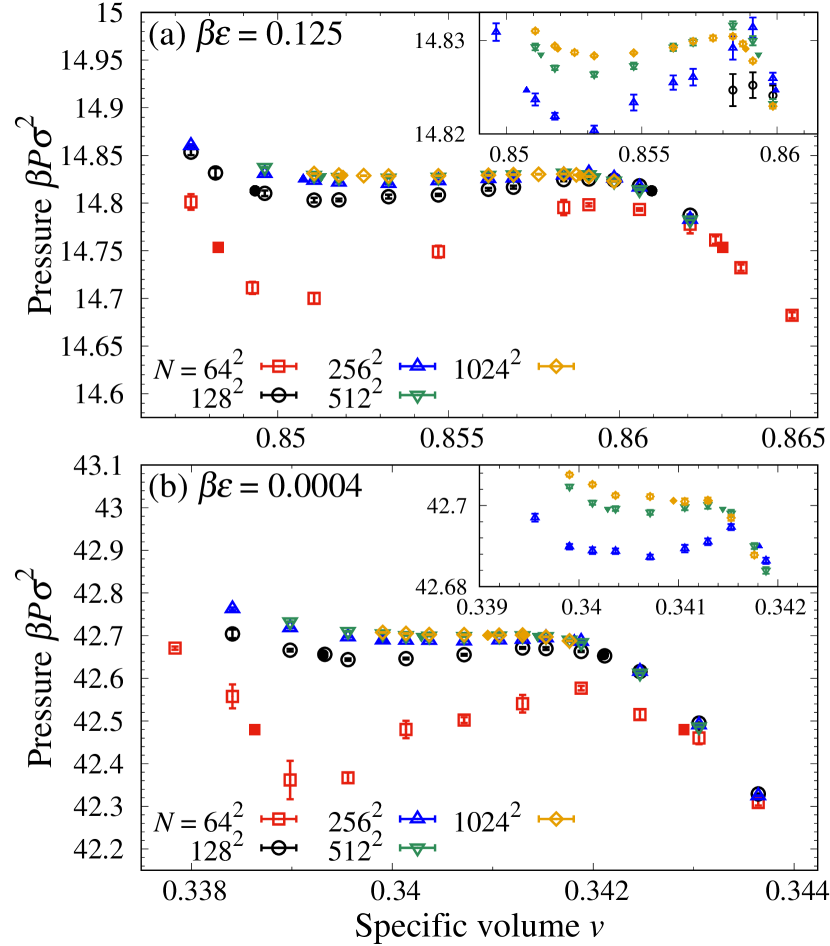
Figure 3: Equation of state of the WCA model at (a) $\beta\epsilon=0.125$ and (b) $\beta\epsilon=0.0004$. Each inset shows the equation of state close to the liquid–hexatic transition. Filled symbols for each system size indicate the specific volumes of the liquid and hexatic phases, $v_{\text{liq}}$ and $v_{\text{hex}}$ ($v_{\text{liq}}>v_{\text{hex}}$).

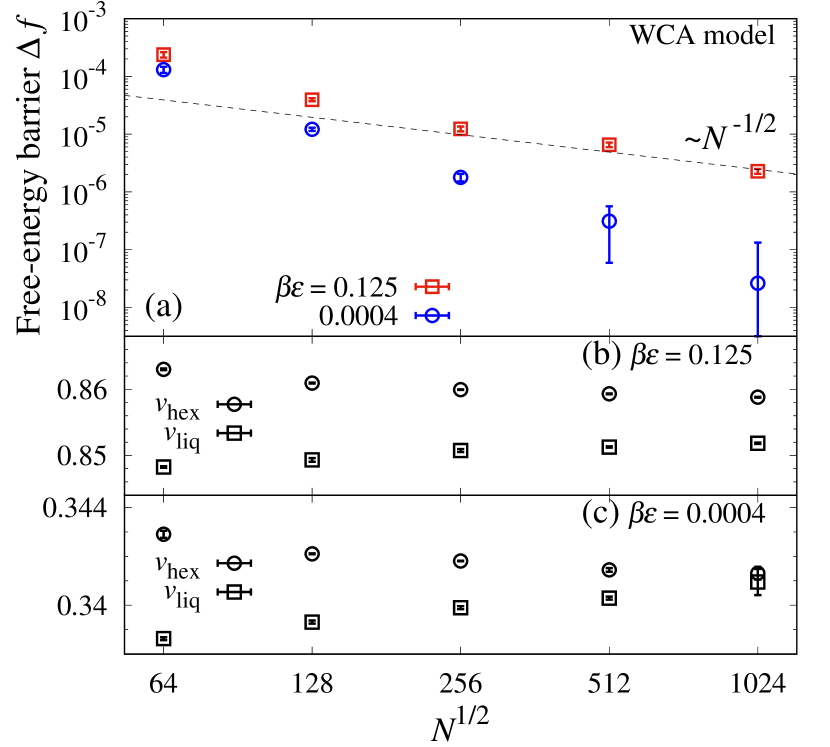
Figure 4: Free-energy barrier $\Delta f$ as a function of $N^{1/2}$ for the WCA model at $\beta\epsilon=0.125$ and $\beta\epsilon=0.0004$. At $\beta\epsilon=0.125$, the free-energy barrier $\Delta f$ crosses over to scaling in $N^{-1/2}$ for large $N$, suggesting a first-order transition. $\Delta f$ decays faster at $\beta\epsilon=0.0004$, implying that the transition is continuous. Specific volumes $v_{\text{liq}}$ and $v_{\text{hex}}$ as functions of $N^{1/2}$, at (b): $\beta\epsilon=0.125$ and (c): $\beta\epsilon=0.0004$. At $\beta\epsilon=0.125$, the specific volumes do not merge while at $\beta\epsilon=0.0004$, they converge to almost the same value at $N=1024^{2}$.

In Section III, we confirmed that the $m=12$ power-law potential has a continuous liquid–hexatic transition. Because the Lennard-Jones model has the same behavior at small separations, it must obey the same continuous liquid–hexatic scenario at high enough temperatures. However, it was recently claimed that the transition is first-order at all temperatures [12, 36]. In this section, we investigate this point with the help of the truncated Lennard-Jones model Eq. (3) which, at high temperature or high density, is equivalent to the Lennard-Jones and the $m=12$ power-law model. We study the WCA model at $\beta\epsilon=0.125$ and $0.0004$. At low temperatures, effects due to the truncation should be strong. We expect that the small value of the cutoff pushes the system to a first-order liquid–hexatic transition. At high temperatures, the effect of truncation is negligible and the WCA model should agree with what is observed in the power-law model for $m=12$.

At low temperature $\beta\epsilon=0.125$, the WCA equation of state features a clear Mayer–Wood loop (see Fig. 3 (a)), and the amplitude decreases with increasing system size. The free-energy barrier $\Delta f$ decays faster than the scaling of the first-order transition, $\Delta f\sim N^{-1/2}$, when $N$ is small, but it approaches this scaling when $N\gtrsim 256^{2}$, Fig. 4 (a) (see also [47], at $\beta\epsilon=1$). The specific volumes $v_{\text{liq}}$ and $v_{\text{hex}}$ are well separated (see Fig. 4 (b)), and the coexisting phase appears between $v_{\text{liq}}\simeq 0.86$ and $v_{\text{hex}}\simeq 0.85$, confirming a first-order transition of the WCA model at low temperature.

At high temperature $\beta\epsilon=0.0004$, the WCA-model equation of state features a loop at $0.34\lesssim v\lesssim 0.342$ for small system sizes, but its amplitude decreases rapidly, and it vanishes for $N\gtrsim 512^{2}$, Fig. 3 (b). The free-energy barrier $\Delta f$ decays faster than the first-order scaling $\Delta f\sim N^{-1/2}$. Consistently, $v_{\text{liq}}$ and $v_{\text{hex}}$ merges at $N\simeq 1024^{2}$, meaning that the system does not have a coexisting phase, see Fig. 4 (c). We thus conclude that, at high enough temperatures, the transition in the WCA model becomes continuous as expected from our results of the $m=12$ model, contrary to the phase diagram shown in Refs. [12, 36].

For the WCA model, the critical inverse temperature $\beta_{c}$ separating the continuous and first-order liquid–hexatic transitions lies in the range $\beta_{c}\epsilon\in(0.0004,0.125)$. These results are consistent with Refs. [12, 36] who, for the Lennard-Jones model, did not observe a continuous transition at inverse temperature $\beta\epsilon=10$, but are inconsistent with $\beta_{c}\epsilon\simeq 0.91$ claimed in Refs. [34, 35],

V Summary and Discussion

We have studied the equation of state of two-dimensional soft disks with power-law interactions and for the WCA model, with its specifically truncated Lennard-Jones interaction. A massively parallel Metropolis algorithm allowed us to study up to $N=1024^{2}$ disks at densities around the liquid–hexatic phase transition and to estimate the equilibrium pressure with high precision. We identified the nature of the phase transition by the scaling of the free-energy barrier with system size. Our results show that the order of the phase transition depends on the exact form of the potentials and, for the WCA model, on temperature. We found that the power-law model with $m=24$ has a first-order phase transition, consistent with the previous study [10]. For softer interactions, $m=12$ and $m=8$, however, the phase transition is continuous. Whereas we find easily that the $m=8$ model has a continuous transition from the monotonic equation of state, the $m=12$ model requires a careful analysis of the system-size dependence to demonstrate its continuous nature: This model has a tiny but clear loop up to $N\simeq 256^{2}$, and the equation of state becomes strictly monotonic only for $N\gtrsim 512^{2}$. The continuous nature of the $m=12$ model is consistent with the conclusion in Ref. [34]. The difference between the cases $m=24$ and $m=12$ clearly appears in the system-size dependence of the free-energy barrier $\Delta f$. We conclude that the parameter $m$ of the power-law model changes the nature of the transition, but the critical value of $m$ separating the two regimes is between $m=12$ and $24$, not $m\lesssim 6$ reported previously [10].

In the WCA model, temperature plays an analogous role to $m$ in the power-law model in changing the nature of the phase transition. At low temperatures, as for $\beta\epsilon=0.125$, the scaling of the free-energy barrier $\Delta f$ indicates a first-order transition. At high temperature, on the other hand, the transition becomes continuous, with finite-size effects that resemble those of the power-law model with $m=12$. A remaining puzzle is the value of the critical temperature $T_{c}$ separating the first-order and continuous liquid–hexatic transitions: Our Monte Carlo data on the WCA model indicate the critical transition between $\beta\epsilon=0.0004$ and $0.125$, while in the conventional Lennard-Jones model it was claimed to be around $\beta_{c}\epsilon\simeq 0.91$ [34, 35], in disagreement with Ref. [36] which states that conventional Lennard-Jones at $\beta\epsilon=0.1$ has a first-order liquid–hexatic transition. This could be either because the truncation in the WCA model shifts the critical temperature, or because tiny but finite loop amplitudes at high temperatures were missed due to statistical noise in Refs. [34, 35]. We will address this issue in future work.

The controversy over the two-dimensional melting transition has originated in two difficulties. First, the very long timescales needed to reach equilibrium at high density and low temperature, and secondly, strong finite-size effects in the equation of state. The former difficulty was partially resolved through event-chain Monte Carlo and massively parallel Metropolis algorithms. The latter, however, is still a source of difficulty. The strong finite-size effects usually originate from a large length scale. We expect the orientational correlation length should not be responsible although it diverges at the continuous liquid–hexatic transition. We have not identified this length scale yet, and will study this length scale in future work.

Appendix A Software package: outline, license, access

The present paper is accompanied by the SoftDisks data and software package, which is published as an open-source project under the GNU GPLv3 license. SoftDisks is available on GitHub as part of the JeLLyFysh organization . The package contains a C++ program, using Nvidia GPU extensions, which implements the massively parallel algorithm of soft-disk model. This program is accompanied by Python scripts for the analysis of data. The package also provides original pressure data for equations of state from Ref. [10], together with those obtained in the present work.

The SoftDisks software package follows Ref. [40]. We overlay the full 2D system with a four-color checkerboard of cells, each containing a small number of disks. Different cells of the same color are separated by more than the cutoff of the potential so that the Metropolis algorithm runs independently on each of them. Monte Carlo trials that move a disk out of its cell are rejected. After a fixed number of cycles (typically $16$), the cell system is displaced randomly. This permits disks to eventually move throughout the system, as required for irreducibility. During simulations, we measure physical quantities, such as the energy and the pressure, which are calculated as sums within the local environment. We also store snapshots of the system for later analysis. Our GPU-based code will be useful for further study of two-dimensional melting.

The Python scripts read the data from a simulation, and perform a detailed analysis of thermodynamic properties. Snapshots are used to generate detailed movies of the time evolution of the system. Our analysis code calculates spatial correlations and Voronoi tessellations using NumPy and SciPy. Equilibrium configurations obtained in this work are available from https://doi.org/10.5281/zenodo.7844567.

References

- Liu et al. [2005] C. Liu, S. Yamazaki, R. Hobara, I. Matsuda, and S. Hasegawa, Atomic scale observation of a two-dimensional liquid-solid phase transition on the Si(111)––Ag surface, Phys. Rev. B 71, 041310 (2005).
- Negulyaev et al. [2009] N. N. Negulyaev, V. S. Stepanyuk, L. Niebergall, P. Bruno, M. Pivetta, M. Ternes, F. Patthey, and W.-D. Schneider, Melting of Two-Dimensional Adatom Superlattices Stabilized by Long-Range Electronic Interactions, Phys. Rev. Lett. 102, 246102 (2009).
- Kusner et al. [1994] R. E. Kusner, J. A. Mann, J. Kerins, and A. J. Dahm, Two-stage melting of a two-dimensional collodial lattice with dipole interactions, Phys. Rev. Lett. 73, 3113 (1994).
- Ebert et al. [2009] F. Ebert, P. Dillmann, G. Maret, and P. Keim, The experimental realization of a two-dimensional colloidal model system, Rev. Sci. Instrum. 80, 083902 (2009).
- Thorneywork et al. [2017] A. L. Thorneywork, J. L. Abbott, D. G. A. L. Aarts, and R. P. A. Dullens, Two-Dimensional Melting of Colloidal Hard Spheres, Phys. Rev. Lett. 118, 158001 (2017).
- Nishikawa et al. [2019] Y. Nishikawa, K. Hukushima, and W. Krauth, Solid-liquid transition of skyrmions in a two-dimensional chiral magnet, Phys. Rev. B 99, 064435 (2019).
- Reichhardt et al. [2022] C. Reichhardt, C. J. O. Reichhardt, and M. V. Milošević, Statics and dynamics of skyrmions interacting with disorder and nanostructures, Rev. Mod. Phys. 94, 035005 (2022).
- Grimes and Adams [1979] C. C. Grimes and G. Adams, Evidence for a Liquid-to-Crystal Phase Transition in a Classical, Two-Dimensional Sheet of Electrons, Phys. Rev. Lett. 42, 795 (1979).
- Glattli et al. [1988] D. C. Glattli, E. Y. Andrei, and F. I. B. Williams, Thermodynamic measurement on the melting of a two-dimensional electron solid, Phys. Rev. Lett. 60, 420 (1988).
- Kapfer and Krauth [2015] S. C. Kapfer and W. Krauth, Two-Dimensional Melting: From Liquid-Hexatic Coexistence to Continuous Transitions, Phys. Rev. Lett. 114, 035702 (2015).
- Anderson et al. [2017] J. A. Anderson, J. Antonaglia, J. A. Millan, M. Engel, and S. C. Glotzer, Shape and Symmetry Determine Two-Dimensional Melting Transitions of Hard Regular Polygons, Phys. Rev. X 7, 021001 (2017).
- Li and Ciamarra [2020a] Y.-W. Li and M. P. Ciamarra, Attraction tames two-dimensional melting: From continuous to discontinuous transitions, Phys. Rev. Lett. 124, 218002 (2020a).
- Peierls [1935] R. Peierls, Quelques propriétés typiques des corps solides, Ann. Henri Poincaré 5, 177 (1935).
- Mermin [1968] N. D. Mermin, Crystalline Order in Two Dimensions, Phys. Rev. 176, 250 (1968).
- Richthammer [2007] T. Richthammer, Translation-invariance of two-dimensional gibbsian point processes, Commun. Math. Phys. 274, 81 (2007).
- Mermin and Wagner [1966] N. D. Mermin and H. Wagner, Absence of Ferromagnetism or Antiferromagnetism in One- or Two-Dimensional Isotropic Heisenberg Models, Phys. Rev. Lett. 17, 1133 (1966).
- Kosterlitz and Thouless [1973] J. M. Kosterlitz and D. J. Thouless, Ordering, metastability and phase transitions in two-dimensional systems, J. Phys. C: Solid State Phys. 6, 1181 (1973).
- Fröhlich and Spencer [1981] J. Fröhlich and T. Spencer, The Kosterlitz-Thouless transition in two-dimensional Abelian spin systems and the Coulomb gas, Commun. Math. Phys. 81, 527 (1981).
- Hasenbusch [2005] M. Hasenbusch, The two-dimensional XY model at the transition temperature: a high-precision Monte Carlo study, J. Phys. A: Math. Gen. 38, 5869 (2005).
- Kosterlitz [2016] J. M. Kosterlitz, Kosterlitz–Thouless physics: a review of key issues, Rep. Prog. Phys. 79, 026001 (2016).
- Nelson [1978] D. R. Nelson, Study of melting in two dimensions, Phys. Rev. B 18, 2318 (1978).
- Nelson and Halperin [1979] D. R. Nelson and B. I. Halperin, Dislocation-mediated melting in two dimensions, Phys. Rev. B 19, 2457 (1979).
- Young [1979] A. P. Young, Melting and the vector Coulomb gas in two dimensions, Phys. Rev. B 19, 1855 (1979).
- Fisher et al. [1979] D. S. Fisher, B. I. Halperin, and R. Morf, Defects in the two-dimensional electron solid and implications for melting, Phys. Rev. B 20, 4692 (1979).
- Chui [1983] S. T. Chui, Grain-boundary theory of melting in two dimensions, Phys. Rev. B 28, 178 (1983).
- Metropolis et al. [1953] N. Metropolis, A. W. Rosenbluth, M. N. Rosenbluth, A. H. Teller, and E. Teller, Equation of State Calculations by Fast Computing Machines, J. Chem. Phys. 21, 1087 (1953).
- Alder and Wainwright [1962] B. J. Alder and T. E. Wainwright, Phase Transition in Elastic Disks, Phys. Rev. 127, 359 (1962).
- Li et al. [2022] B. Li, Y. Nishikawa, P. Höllmer, L. Carillo, A. C. Maggs, and W. Krauth, Hard-disk pressure computations—a historic perspective, J. Chem. Phys. 157, 234111 (2022).
- Bernard and Krauth [2011] E. P. Bernard and W. Krauth, Two-Step Melting in Two Dimensions: First-Order Liquid-Hexatic Transition, Phys. Rev. Lett. 107, 155704 (2011).
- Engel et al. [2013] M. Engel, J. A. Anderson, S. C. Glotzer, M. Isobe, E. P. Bernard, and W. Krauth, Hard-disk equation of state: First-order liquid-hexatic transition in two dimensions with three simulation methods, Phys. Rev. E 87, 042134 (2013).
- Strandburg et al. [1984] K. J. Strandburg, J. A. Zollweg, and G. V. Chester, Bond-angular order in two-dimensional Lennard-Jones and hard-disk systems, Phys. Rev. B 30, 2755 (1984).
- Chen et al. [1995] K. Chen, T. Kaplan, and M. Mostoller, Melting in Two-Dimensional Lennard-Jones Systems: Observation of a Metastable Hexatic Phase, Phys. Rev. Lett. 74, 4019 (1995).
- Wierschem and Manousakis [2011] K. Wierschem and E. Manousakis, Simulation of melting of two-dimensional Lennard-Jones solids, Phys. Rev. B 83, 214108 (2011).
- Hajibabaei and Kim [2019] A. Hajibabaei and K. S. Kim, First-order and continuous melting transitions in two-dimensional Lennard-Jones systems and repulsive disks, Phys. Rev. E 99 (2019).
- Toledano et al. [2021] O. Toledano, M. Pancorbo, J. E. Alvarellos, and O. Gálvez, Melting in two-dimensional systems: Characterizing continuous and first-order transitions, Phys. Rev. B 103, 094107 (2021).
- Li and Ciamarra [2020b] Y.-W. Li and M. P. Ciamarra, Phase behavior of Lennard-Jones particles in two dimensions, Phys. Rev. E 102, 062101 (2020b).
- Zahn et al. [1999] K. Zahn, R. Lenke, and G. Maret, Two-Stage Melting of Paramagnetic Colloidal Crystals in Two Dimensions, Phys. Rev. Lett. 82, 2721 (1999).
- Mayer and Wood [1965] J. E. Mayer and W. W. Wood, Interfacial Tension Effects in Finite, Periodic, Two-Dimensional Systems, J. Chem. Phys. 42, 4268 (1965).
- Alonso and Fernández [1999] J. J. Alonso and J. F. Fernández, van der Waals loops and the melting transition in two dimensions, Phys. Rev. E 59, 2659 (1999).
- Anderson et al. [2013] J. A. Anderson, E. Jankowski, T. L. Grubb, M. Engel, and S. C. Glotzer, Massively parallel Monte Carlo for many-particle simulations on GPUs, J. Comput. Phys. 254, 27 (2013).
- Weeks et al. [1971] J. D. Weeks, D. Chandler, and H. C. Andersen, Role of Repulsive Forces in Determining the Equilibrium Structure of Simple Liquids, J. Chem. Phys. 54, 5237 (1971).
- Kapfer and Krauth [2016] S. C. Kapfer and W. Krauth, Cell-veto Monte Carlo algorithm for long-range systems, Phys. Rev. E 94, 031302 (2016).
- Smit and Frenkel [1991] B. Smit and D. Frenkel, Vapor–liquid equilibria of the two-dimensional Lennard-Jones fluid(s), J. Chem. Phys. 94, 5663 (1991).
- Smit [1992] B. Smit, Phase diagrams of Lennard-Jones fluids, J. Chem. Phys. 96, 8639 (1992).
- Wittmer et al. [2013a] J. P. Wittmer, H. Xu, P. Polińska, F. Weysser, and J. Baschnagel, Shear modulus of simulated glass-forming model systems: Effects of boundary condition, temperature, and sampling time, J. Chem. Phys. 138, 12A533 (2013a).
- Wittmer et al. [2013b] J. P. Wittmer, H. Xu, P. Polińska, C. Gillig, J. Helfferich, F. Weysser, and J. Baschnagel, Compressibility and pressure correlations in isotropic solids and fluids, Eur. Phys. J. E 36, 131 (2013b).
- Khali et al. [2021] S. S. Khali, D. Chakraborty, and D. Chaudhuri, Two-step melting of the Weeks–Chandler–Anderson system in two dimensions, Soft Matter 17, 3473 (2021).
- Politis and Romano [1994] D. N. Politis and J. P. Romano, The Stationary Bootstrap, J. Am. Stat. Assoc. 89, 1303 (1994).
- Politis and White [2004] D. N. Politis and H. White, Automatic Block-Length Selection for the Dependent Bootstrap, Econom. Rev. 23, 53 (2004).
- Patton et al. [2009] A. Patton, D. N. Politis, and H. White, Correction to “Automatic Block-Length Selection for the Dependent Bootstrap” by D. Politis and H. White, Econom. Rev. 28, 372 (2009).
- Nishikawa et al. [2021] Y. Nishikawa, J. Takahashi, and T. Takahashi, Stationary bootstrap: A refined error estimation for equilibrium time series (2021), arXiv:2112.11837 .
- Binder et al. [2012] K. Binder, B. J. Block, P. Virnau, and A. Tröster, Beyond the Van Der Waals loop: What can be learned from simulating Lennard-Jones fluids inside the region of phase coexistence, Am. J. Phys. 80, 1099 (2012).
- Halperin and Nelson [1978] B. I. Halperin and D. R. Nelson, Theory of Two-Dimensional Melting, Phys. Rev. Lett. 41, 121 (1978).
- Note [1] The url of repository is https://github.com/jellyfysh/SoftDisks.