Traffic signal optimization using quantum annealing on real map

Abstract

The quantum annealing machine manufactured by D-Wave Systems is expected to find the optimal solution for QUBO (Quadratic Unconstrained Binary Optimization) accurately and quickly. This would be useful in future applications where real-time calculation is needed. One such application is traffic signal optimization. Some studies use quantum annealing for this. However, they are formulated in unrealistic settings, such as only crossroads on the map. Therefore, we suggest a QUBO, which can deal with T-junctions and multi-forked roads. To validate the efficiency of our approach, SUMO (Simulation of Urban MObility) is used. This enables us to experiment with geographic information data very close to the real world. We compared results with those using the Gurobi Optimizer in the experiment to confirm that quantum annealing can find a ground state. The results show that the quantum annealing cannot find the ground state, but our model can reduce the time that vehicles wait at a red light. It is also inferior to the Gurobi Optimizer in calculation time. This seems to be due to the D-Wave machine’s hardware limitations and noise effects, such as ambient temperature. If these problems are solved, and the number of qubits is increased, the use of quantum annealing is likely to be superior in terms of the speed of calculating an optimal solution.

Introduction

D-Wave’s quantum annealing machine has gathered significant attention as the first commercially available device in quantum computing to solve combinatorial optimization problems. Quantum annealing is a method that aims at faster convergence to the optimal state by introducing quantum fluctuations to simulated annealing[1]. D-Wave’s machines are said to be superior, especially for combinatorial optimization problems, and are expected to be useful in many industrial fields. For instance, it can be applied to applications such as traffic flow optimization[2, 3, 4], nurse scheduling problem[5], finance [6, 7], logistics [8], manufacturing [9, 10, 11], preprocessing in material experiments[12], marketing [13], steel manufacturing [10], and decoding problems [14, 15]. The model-based Bayesian optimization is also proposed in the literature [16]. A comparative study of quantum annealer was performed for benchmark tests to solve optimization problems [17]. The quantum effect on the case with multiple optimal solutions has also been discussed [18, 19]. As the environmental effect cannot be avoided, the quantum annealer is sometimes regarded as a simulator for quantum many-body dynamics [20, 21, 22]. Furthermore, applications of quantum annealing as an optimization algorithm in machine learning have also been reported [23, 24, 25, 26, 27, 28, 29, 30, 31].

In the present study, we use quantum annealing for traffic signal optimization. One of the roles of traffic signals is to improve the flow of traffic[32]. Not only does this help vehicles reach their destinations faster, but it also reduces traffic pollution[33], such as exhaust emissions and noise. Nowadays, traffic-sensitive control is used at intersections with particularly heavy traffic in Japan[34]. This method involves transmitting real-time traffic volume to a control center, which calculates and sends back the appropriate signal lighting times. This method eliminates traffic congestion more flexibly than fixed-cycle control, which always repeats the same lighting time. On the other hand, it also has the disadvantage that the amount of calculation increases exponentially as the number of intersections to be controlled increases. High-speed computation is demanded since real-time calculation is required for traffic signal optimization. We focus on the potential of the quantum annealing machine manufactured by D-Wave Systems. Some previous studies use the quantum annealer but have not been formulated and experimented in realistic settings. The study by Inoue et al.[35] defines only two intersection states; the green light indicates the north-south direction, and the traffic light in the east-west direction exhibits green. Namely, it cannot deal with right-turn-only lanes and multi-forked roads. The study by Hussain et al.[36] is more realistic because it defines six intersection states, including right-turn signals etc. However, all intersections are assumed to be cross streets, which is impractical. In addition, the simulation was performed on a square grid, and the road lengths and other settings deviated from the real world. The cost function is designed to allow vehicles to pass through intersections continuously, but the simulation results show little difference from local control, which does not consider this. In other words, there may be a problem in the formulation. Therefore, in this study, we formulate a QUBO that can eliminate congestion better than local control in a realistic setting that can deal with T-junctions, multiple-junction roads, and multiple lanes. We also propose a method that is completely different from existing studies[36], which can reduce traffic congestion compared to the local control.

However, to use D-Wave’s machine, problems must be described in a specific format, namely the QUBO (Quadratic Unconstrained Binary Optimization) format [37]. Converting real-world problems into this format is a necessary step.

The number of qubits available on D-Wave’s machines varies depending on the version. For example, the D-Wave 2000Q, introduced in 2017, offers approximately 2,000 qubits. Subsequently, introduced in 2020, the Advantage system has more than 5000 qubits, providing a significant leap in computational power compared to the previous model. The version of these machines and the number of qubits directly impact their computational speed and adaptability to problems[38]. Besides, the physical qubit connections of a D-Wave machine are not all directly connected. Thus, if the variables in a problem do not match the connection structure of the physical qubits, the variables must be ’embedded’ to represent the problem on the machine. Finding the optimal embedding is sometimes difficult, and the embedding process may require additional qubits or connections. This increases the size and complexity of the problem and can affect the accuracy of the solution search. In addition, D-Wave’s machines are very sensitive to environmental factors such as external temperature fluctuations. These interferences can affect the performance to solve the optimization problem as noise and reduce the accuracy of the computation. Therefore, in this study, we verify whether the current machine provides an optimal solution by comparing the results with those obtained by solving the problem with Gurobi Optimizer[39]. Gurobi Optimizer is a commercial solver that outputs an exact solution.

The remainder of this paper is organized as follows. This section explains the reasons for using quantum annealing for traffic signal optimization and how it differs from previous studies. In the next section, we describe the formulation for eliminating congestion. In the following, we introduce the specific experimental setup and compare the results of that experiment from various perspectives. In the final section, we summarize the study and discuss the usefulness of our approach.

Methods

This section describes the problem set for intersections and identifies the differences from existing methods[36][35]. Next, we formulate the QUBO to reduce traffic congestion.

Preliminary

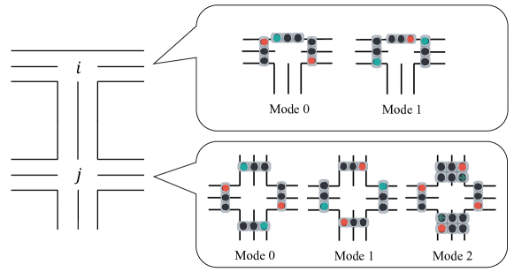
We introduce a variable that has several states at each intersection. For example, as shown in Figure 1, the $i$-th intersection has two different states. Each of these states is called a ’mode’. Let us define $x_{im}$, $1$ when the mode $m$ is chosen at the $i$-th intersection and $0$ otherwise. There is also a mode where only right turns are allowed, such as mode $2$ at the $j$-th intersection. Such as these, the type and number of possible modes vary from intersection to intersection. These settings accurately reflect real intersections.

Figure 1: Examples of modes. $i$-th intersection have two modes and $j$-th intersection have three modes. In mode $2$ of the $j$-th intersection, only vehicles in the right-turn-only lane of the south-north direction can pass through the intersection.

Formulation

Next, we design the cost function to reduce traffic congestion. However, since creating a model that would achieve this directly is difficult, the cost function is divided into three parts. First, we set a cost function to maximize the number of vehicles passing through each intersection.

$$\min_{\vec{x}}\left\{H_{1}(\vec{x})=-\alpha\sum_{i}^{N}\sum_{m\in M_{i}}C_{im}x_{im}\right\},$$ (1)

where $C_{im}$ is the number of vehicles that can pass through the $i$-th intersection if the mode $m$ is also selected, $\alpha$ is the hyper-parameter, $N$ is the number of intersections with traffic signals, and $M_{i}$ is the set of modes that $i$-th intersection has.

$H_{1}$ is the optimal mode selected from the perspective of any intersection. However, if the next intersection cannot be passed continuously, it will not essentially solve the traffic congestion. We then introduce the following term.

$$\min_{\vec{x}}\left\{H_{2}(\vec{x})=-\beta\sum_{i}^{N}\sum_{m\in M_{i}}\sum_{j\in N_{i}}\sum_{n\in M_{j}}B_{ij}R_{im,jn}x_{im}x_{jn}\right\},$$ (2)

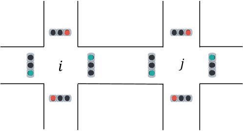
where $\beta$ is the hyper-parameter, $M_{i}$ is the set of adjacent intersections of $i$-th intersection, $B_{ij}$ is the degree of connectivity between $i$ and $j$, and $R_{im,jn}$ represents the relationship when the $i$-th intersection takes the mode $m$ and the $j$-th adjacent intersection takes the $n$-th mode. For example, as shown in Figure 2, when the east-west direction can pass through the $i$-th intersection, vehicles can pass continuously if the same direction is blue at the $j$-th intersection. In this way, there are preferred patterns. In the same way, some unfavorable patterns and patterns are neither. They are defined by $R_{im,jn}$.

$$R_{im,jn}:=\left\{\begin{array}[]{ll}+1&\begin{aligned} \text{If the pattern where }i\text{ takes }m\text{ and }j\text{ takes }n\text{ is favorable .}\end{aligned}\\ 0&\begin{aligned} \text{If the pattern where }i\text{ takes }m\text{ and }j\text{ takes }n\text{ is neither favorable nor unfavorable.}\end{aligned}\\ -1&\begin{aligned} \text{If the pattern where }i\text{ takes }m\text{ and }j\text{ takes }n\text{ is unfavorable.}\end{aligned}\end{array}\right..$$ (3)

Figure 2: A pattern that may be preferred. The $i$-th intersection and the $j$-th intersection select the same mode.

If the preferred pattern is selected, $R_{im,jn}$ will be positive, and the cost will be small. On the other hand, if an unfavorable pattern is selected, the cost will be large. Furthermore, in the case of neither pattern, $R_{im,jn}$ is set to 0 to not affect the cost. Now, how should we determine the relationship parameters? We have map data, traffic volume data, and a traffic simulator. Therefore, we can search in advance for relationship parameters that will reduce traffic congestion. In particular, we use Optuna[40], a tool that can search for parameters by Bayesian optimization. The parameters are prepared as described above.

Next, $B_{ij}$ is defined as follows.

$$B_{ij}:={\text{Speed limit between }i\text{ and }j}/\text{Distance between }i\text{ and }j.$$ (4)

$B_{ij}$ is larger when the distance between $i$ and $j$ is smaller, and the speed limit between $i$ and $j$ is higher. By multiplying $B_{ij}$ and $R_{im,jn}$ together, it is possible to be less concerned about the relationship if it takes time to travel from $i$ to $j$.

Finally, penalty terms are introduced to satisfy the one-hot constraint in the following Equation 5.

$$\min_{\vec{x}}\left\{H_{3}(\vec{x})=\gamma\sum_{i}^{N}\left(\sum_{m\in M_{i}}x_{im}-1\right)^{2}\right\},$$ (5)

where $\gamma$ is a hyper-parameter. The final cost function to be solved is as follows.

$$H(\vec{x})=H_{1}(\vec{x})+H_{2}(\vec{x})+H_{3}(\vec{x}).$$ (6)

By solving Equation 6, the mode that as many vehicles as possible can proceed is chosen at each intersection. In contrast, the preferred mode is chosen at adjacent intersections to make traffic smoother. In the following section, we will validate whether the optimal solution of Equation 6 can alleviate traffic congestion within the simulator.

Problem settings

SUMO(Simulation of Urban MObility)[41] is an open software program that allows users to download terrain data from open street maps and drive their vehicles on them. The map used is shown in the following Figure 3.

Figure 3: Map used for simulation. We utilized a portion of Aomori City. This map includes multi-forked roads and multi-lane intersections. Intersections with traffic signals are marked with a traffic light symbol.

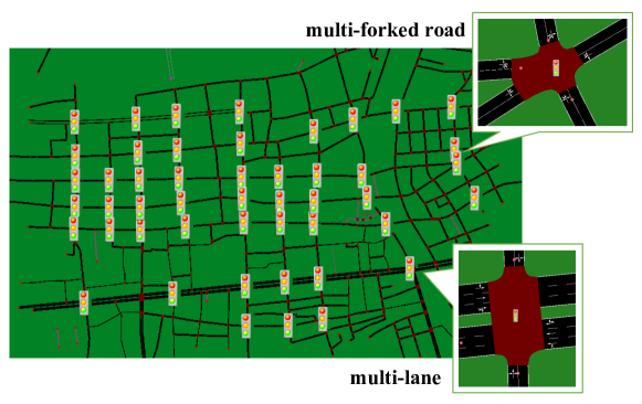
For this experiment, we utilized a portion of Aomori City in the northernmost region of Japan’s main island, Honshu. Aomori City is a relatively heavy-traffic area in Aomori Prefecture. On this map, multi-forked roads and multi-lanes are included. Intersections with traffic signals are marked with a traffic signal symbol. There are $48$ signalized intersections on this map. Since each intersection has two or three modes, the number of binary variables is $100$. In addition, obtaining a true data set for traffic volume data is difficult. Thus, we randomly determined the destination of vehicles in this simulation. The number of vehicles is set to $1000$, and vehicles arriving at their destinations are excluded from the map. The experiment is conducted in the following two steps.

Step1

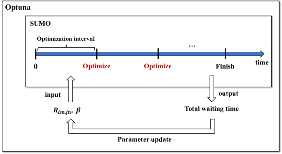
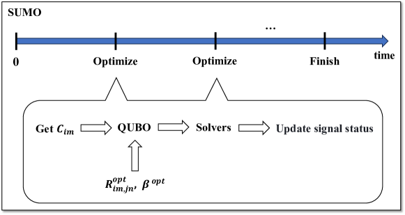
By using map data and traffic volume data, the optimal parameters are searched for in advance. An overview is shown in the following Figure 4. Within SUMO, optimization was performed every 20 seconds. After 400 seconds, the simulation was stopped, and the time the vehicles waited at the red light was measured. The reason for the longer optimization interval is to prevent frequent signal switching. If this interval were to be shortened, an additional penalty term would need to be included in QUBO. This is supplemented in the next subsection. In Optuna, the parameters to be explored are input to SUMO. Next, the parameters are searched so that the output from SUMO becomes smaller. This was repeated 100 times.

Figure 4: Overview of Step1.

Step2

Next, by using the acquired hyper-parameters, we compare different solvers. These solvers are quantum annealing, simulated annealing, and Gurogi Optimizer. For quantum annealing, we used the D-Wave Advantage system 4.1. We used the SASampler from OpenJij for simulated annealing to compare quantum annealing with the calculation time. We also compare the results of solving only $H_{1}+H_{3}$ (which we call ’local’ control) using Gurobi. This is to check the contribution of the relationship parameters. An overview is shown in the following Figure 5.

Figure 5: Overview of Step2.

In the next subsection, we explain why we set a longer optimization interval, as described in Step1.

Optimazation interval

In actual traffic signals, pedestrians have minimum time to cross a pedestrian crossing safely. Therefore, frequent signal changes cause safety problems. If the optimization interval is to be shortened, the following Equation 7 should be added to QUBO.

$$H_{4}(\vec{x}) =\begin{cases}\sum_{i}^{N}\left(\sum_{m\in M_{i}}x_{im}+\tau_{im}-T_{i}\right)^{2}&\text{if }\tau_{im}<T_{i}\\ 0&\text{if }\tau_{im}\geq T_{i}\end{cases},$$ (7)

where $\tau_{im}$ is the duration time that the mode $m$ has been chosen continuously at the $i$-th intersection from when the mode was switched to the current time. $T_{i}$ is the time required for a pedestrian to cross the pedestrian crossing at $i$-th intersection. For short intervals, $H=H_{1}+H_{2}+H_{3}+H_{4}$ must be solved. The crosswalk length and other factors determine the value of $T_{i}$. This value is difficult to obtain with the simulator used in this study and is not considered.

The next section shows the results of solving $H=H_{1}+H_{2}+H_{3}$ every 20 seconds. First, we introduce the relationship parameters obtained. Next, the solvers are compared for the waiting time at the red light, the calculation time, and the number of vehicles on the map.

Results

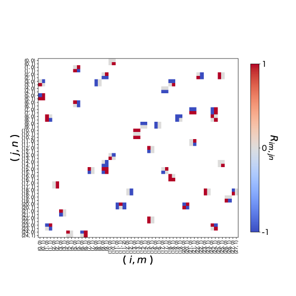
First, the parameters obtained in Step1 are shown in Figure 6. It can be seen that the values are not all zero. In other words, there are indeed favorable and unfavorable patterns between $i$, $m$, $j$, and $n$.

Figure 6: Optimized parameters. $\beta$ was searched from 0.01 to 1.0 in increments of 0.01. As a result, $\beta$ is 0.05.

Next, we confirm that the proposed QUBO can eliminate traffic congestion. In this study, the waiting time at the red light is used as an indicator of eliminating traffic congestion. The result of comparing total waiting time using the acquired relationship parameters is shown in Figure 7.

Figure 7: Total waiting time for each method. QA denotes the results of quantum annealing, SA represents simulated annealing, Gurobi stands for those of Gurobi Optimizer, Local is a method for solving $H_{1}+H_{3}$, and Fixed is a method for repeating constant lighting time. Ten simulations were conducted for SA and QA, plotting the average values. Error bars are standard deviations, but they were not plotted for Gurobi, Local, and Fixed because the results are always the same. We set $\alpha=1.0,\gamma=10.0$.

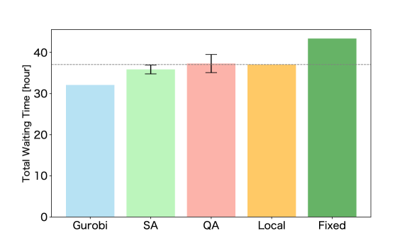
In the case of local control, the total waiting time is about 37 hours, and in the case of Gurobi, it is about 32 hours. In other words, it can be shown that the introduction of the relationship parameter has reduced the waiting time by about 13%. On the other hand, the average value of QA is 37 hours. Comparing this with Gurobi’s results shows that QA does not require an optimal solution. Furthermore, since the standard deviation of QA is about 2.2 hours, it is clear that a solution with low energy cannot be output consistently.

Next, a comparison of calculation times is conducted. The computations were performed on a MacBook Pro, a 13-inch 2020 model. The chip used is the Apple M1, with 16GB of memory. The operating system is macOS Ventura 13.4.1.

Figure 8: Calculation time log for each method. Ten simulations were conducted for Gurobi, SA, and QA, plotting the average values. Error bars are standard deviations.

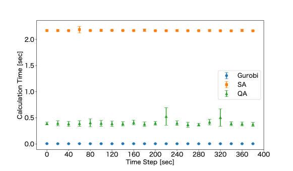
Figure7 shows the results of comparing calculation times. Two methods, SA and QA, are sampled 1000 times, and the solution with the lowest energy is adopted. Here, the annealing time for QA is 10 $\mu$s, and the number of Monte Carlo steps in SA is 1000. QA also includes the communication time with Canada, where the machine is located, and it is slower than Gurobi but superior to SA.

Finally, we compare the number of vehicles on the map. The more vehicles on the map, the more congestion can occur. The results are shown in Figure9.

Figure 9: Number of vehicles on the map for each method. Ten simulations were conducted for SA and QA, and the average values were plotted. Error bars are standard deviations, but for Gurobi and Fixed, they were not plotted because the results are always the same.

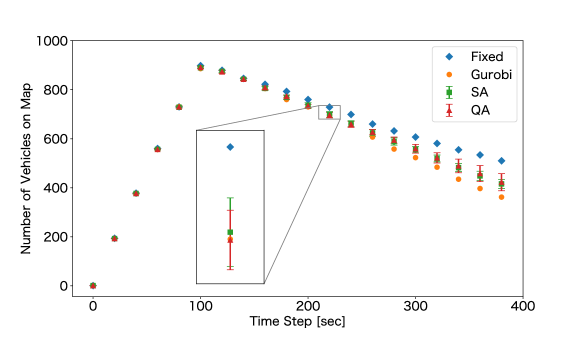
From zero to 100 seconds, we set the inflow to 1000 vehicles on the map. Thus, as shown in Figure9, the number of vehicles continues to increase until 100 seconds. During this period, there is little difference between Solvers. However, once the influx of vehicles calmed, it became clear that Gurobi could reduce the number of vehicles the most, followed by SA, QA, and Fixed. This order is the same as the result of the total waiting time.

The next section discusses why QA can not reduce traffic congestion. Next, another approach to parameter search will be discussed.

Discussion

As shown in Figure 7, it can be seen that QA does not obtain a solution with lower energy than Gurobi and SA. This may be due to the effects of embedding and noise. Another reason may be that the internal parameters of the D-Wave machine are not well adjusted. The default annealing time is 20 microseconds, but a longer annealing time will likely give better solutions. In addition, the D-Wave machine has a function called reverse annealing. In this technique, the classical solution is taken as the initial state. Next, the transverse magnetic field is gradually applied from the state where it is turned off, and finally, it is turned off again. This allows us to search for a better solution. Haba’s study[11] has shown that reverse annealing makes it easier to obtain the ground state.

As for computation time, QA is not as good as Gurobi. However, Hirama’s study [42] has shown that as the data size increases, the computation time becomes faster than Gurobi. In particular, their method improves performance when the number of constraints increases. Quantum annealing machines can deal with more realistic constraints with their method. Therefore, in the future, when the number of available qubits increases, and the effect of embedding is reduced, there is a potential to obtain the ground state in a faster computation time than Gurobi even for practical problem setting as studied in the present study.

Finally, we discuss the parameter search. In the experiment described above, all relationship parameters are searched simultaneously. However, the cost function only defines the relationship between adjacent intersections. Hence, we considered that a parameter search focused on adjacent intersections and finally merged parameters would give better results for each intersection. We then search for such an approach. All relationship parameters are fixed to $0$ except for the target parameter. Ten searches were conducted for each intersection, giving 280 searches. The following Figure 10 shows the results of measuring the waiting time using the parameters obtained from this approach.

Figure 10: Total waiting time for each method. ’Search for each’ and ’Local’ are the same results as in Figure 7. ’Search for all’ is the result we want to examine in this section. Since all of these methods output the same results, only one simulation was conducted and error bars were not plotted.

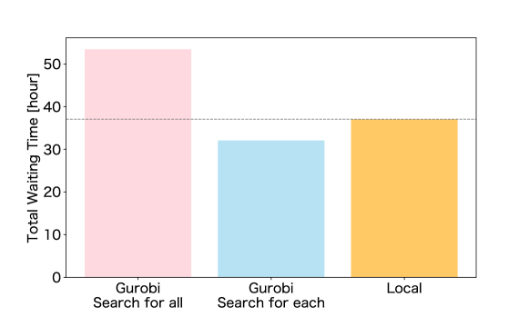
Contrary to expectations, ’Search for all’ results are worse than local control. This result may suggest that a relationship with non-adjacent intersections is also important. That is, defining the relationship between non-adjacent intersections may give better results. Furthermore, the relationship at each time step could also be defined. However, as the number of parameters increases, the difficulty of the search will increase, and generalization performance will decrease.

In this study, we proposed the method using quantum annealing for traffic signal optimization, which requires real-time computation. In previous studies, experiments are conducted in impractical settings. It is difficult to apply them to the real world. Therefore, in this study, we formulated the QUBO in a realistic setting that can be applied to the actual world, and by using SUMO in the experiments, we conducted simulations using real map data. As a result, quantum annealing cannot find the optimal solution, and the computation speed is slower than Gurobi. However, the results of Gurobi show that our formulation can eliminate traffic congestion even in practical situations. With the present D-Wave’s machines, the accuracy of solution search can be improved by adjusting internal parameters and using techniques such as reverse annealing. On the other hand, the effects of embedding and other factors cannot be avoided. In addition, it is inferior to Gurobi in terms of computation speed. However, some studies have shown that the larger the problem size, the faster the D-Wave machine is in terms of computation speed [42]. In the future, D-Wave’s machines are expected to use more qubits and be less affected by embedding and noise. When this is realized, the use of quantum annealing may be advantageous in terms of the speed of calculating the optimal solution.

Author contributions statement

R. S. conceived the experiments, conducted the experiments, and analyzed the results. M. O. supervised the conduct of this study. All authors reviewed the manuscript draft and revised it critically on intellectual content. All authors approved the final version of the manuscript to be published.

Additional information

Competing interests. The authors have no competing interests to disclose.

References

- [1] Kadowaki, T. & Nishimori, H. Quantum annealing in the transverse Ising model. \JournalTitlePhysical Review E 58, 5355–5363, DOI: 10.1103/PhysRevE.58.5355 (1998). Publisher: American Physical Society.
- [2] Neukart, F. et al. Traffic flow optimization using a quantum annealer. \JournalTitleFront. ICT 4, 29 (2017).
- [3] Hussain, A., Bui, V.-H. & Kim, H.-M. Optimal sizing of battery energy storage system in a fast ev charging station considering power outages. \JournalTitleIEEE Transactions on Transportation Electrification 6, 453–463 (2020).
- [4] Inoue, D., Okada, A., Matsumori, T., Aihara, K. & Yoshida, H. Traffic signal optimization on a square lattice with quantum annealing. \JournalTitleScientific reports 11, 1–12 (2021).
- [5] Ikeda, K., Nakamura, Y. & Humble, T. S. Application of Quantum Annealing to Nurse Scheduling Problem. \JournalTitleScientific Reports 9, 12837, DOI: 10.1038/s41598-019-49172-3 (2019). Number: 1 Publisher: Nature Publishing Group.
- [6] Rosenberg, G. et al. Solving the optimal trading trajectory problem using a quantum annealer. \JournalTitleIEEE J. Sel. Top. Signal Process. 10, 1053–1060 (2016).
- [7] Venturelli, D. & Kondratyev, A. Reverse quantum annealing approach to portfolio optimization problems. \JournalTitleQuantum Machine Intelligence 1, 17–30 (2019).
- [8] Mugel, S. et al. Dynamic Portfolio Optimization with Real Datasets Using Quantum Processors and Quantum-Inspired Tensor Networks. \JournalTitlePhysical Review Research 4, 013006, DOI: 10.1103/PhysRevResearch.4.013006 (2022). ArXiv:2007.00017 [quant-ph, q-fin].
- [9] Venturelli, D., Marchand, D. J. J. & Rojo, G. Quantum annealing implementation of job-shop scheduling (2016). 1506.08479.
- [10] Yonaga, K. et al. Quantum optimization with lagrangian decomposition for multiple-process scheduling in steel manufacturing. \JournalTitleISIJ International 62, 1874–1880, DOI: 10.2355/isijinternational.ISIJINT-2022-019 (2022).
- [11] Haba, R., Ohzeki, M. & Tanaka, K. Travel time optimization on multi-agv routing by reverse annealing. \JournalTitleScientific Reports 12, 17753, DOI: 10.1038/s41598-022-22704-0 (2022).
- [12] Tanaka, T. et al. Virtual screening of chemical space based on quantum annealing. \JournalTitleJournal of the Physical Society of Japan 92, 023001, DOI: 10.7566/JPSJ.92.023001 (2023). https://doi.org/10.7566/JPSJ.92.023001.
- [13] Nishimura, N., Tanahashi, K., Suganuma, K., Miyama, M. J. & Ohzeki, M. Item listing optimization for e-commerce websites based on diversity. \JournalTitleFront. Comput. Sci. 1, 2 (2019).
- [14] Ide, N., Asayama, T., Ueno, H. & Ohzeki, M. Maximum Likelihood Channel Decoding with Quantum Annealing Machine. In 2020 International Symposium on Information Theory and Its Applications (ISITA), 91–95 (2020).
- [15] Arai, S., Ohzeki, M. & Tanaka, K. Mean field analysis of reverse annealing for code-division multiple-access multiuser detection. \JournalTitlePhys. Rev. Research 3, 033006, DOI: 10.1103/PhysRevResearch.3.033006 (2021).
- [16] Koshikawa, A. S., Ohzeki, M., Kadowaki, T. & Tanaka, K. Benchmark test of black-box optimization using d-wave quantum annealer. \JournalTitleJ. Phys. Soc. Jpn. 90, 064001, DOI: 10.7566/JPSJ.90.064001 (2021). https://doi.org/10.7566/JPSJ.90.064001.
- [17] Oshiyama, H. & Ohzeki, M. Benchmark of quantum-inspired heuristic solvers for quadratic unconstrained binary optimization. \JournalTitleSci. Rep. 12, 2146, DOI: 10.1038/s41598-022-06070-5 (2022).
- [18] Yamamoto, M., Ohzeki, M. & Tanaka, K. Fair sampling by simulated annealing on quantum annealer. \JournalTitleJ. Phys. Soc. Jpn. 89, 025002, DOI: 10.7566/JPSJ.89.025002 (2020). https://doi.org/10.7566/JPSJ.89.025002.
- [19] Maruyama, N., Ohzeki, M. & Tanaka, K. Graph minor embedding of degenerate systems in quantum annealing. \JournalTitlearXiv:2110.10930 (2021). 2110.10930.
- [20] Bando, Y. et al. Probing the universality of topological defect formation in a quantum annealer: Kibble-zurek mechanism and beyond. \JournalTitlePhys. Rev. Research 2, 033369, DOI: 10.1103/PhysRevResearch.2.033369 (2020).
- [21] Bando, Y. & Nishimori, H. Simulated quantum annealing as a simulator of nonequilibrium quantum dynamics. \JournalTitlePhys. Rev. A 104, 022607, DOI: 10.1103/PhysRevA.104.022607 (2021).
- [22] King, A. D. et al. Coherent quantum annealing in a programmable 2,000 qubit ising chain. \JournalTitleNature Physics 18, 1324–1328, DOI: 10.1038/s41567-022-01741-6 (2022).
- [23] Neven, H., Denchev, V. S., Rose, G. & Macready, W. G. Qboost: Large scale classifier training withadiabatic quantum optimization. In Asian Conference on Machine Learning, 333–348 (PMLR, 2012).
- [24] Khoshaman, A. et al. Quantum variational autoencoder. \JournalTitleQuantum Science and Technology 4, 014001 (2018).
- [25] O’Malley, D., Vesselinov, V. V., Alexandrov, B. S. & Alexandrov, L. B. Nonnegative/binary matrix factorization with a d-wave quantum annealer. \JournalTitlePloS one 13, e0206653 (2018).
- [26] Amin, M. H., Andriyash, E., Rolfe, J., Kulchytskyy, B. & Melko, R. Quantum Boltzmann Machine. \JournalTitlePhysical Review X 8 (2018). 1601.02036.
- [27] Kumar, V., Bass, G., Tomlin, C. & Dulny, J. Quantum annealing for combinatorial clustering. \JournalTitleQuantum Information Processing 17, 39, DOI: http://doi.org/10.1007/s11128-017-1809-2 (2018).
- [28] Arai, S., Ohzeki, M. & Tanaka, K. Teacher-student learning for a binary perceptron with quantum fluctuations. \JournalTitleJ. Phys. Soc. Jpn. 90, 074002, DOI: 10.7566/JPSJ.90.074002 (2021). https://doi.org/10.7566/JPSJ.90.074002.
- [29] Sato, T., Ohzeki, M. & Tanaka, K. Assessment of image generation by quantum annealer. \JournalTitleSci. Rep. 11, 13523, DOI: 10.1038/s41598-021-92295-9 (2021).
- [30] Urushibata, M., Ohzeki, M. & Tanaka, K. Comparing the effects of boltzmann machines as associative memory in generative adversarial networks between classical and quantum samplings. \JournalTitleJournal of the Physical Society of Japan 91, 074008, DOI: 10.7566/JPSJ.91.074008 (2022). https://doi.org/10.7566/JPSJ.91.074008.
- [31] Hasegawa, Y., Oshiyama, H. & Ohzeki, M. Kernel learning by quantum annealer (2023). 2304.10144.
- [32] Papageorgiou, M., Diakaki, C., Dinopoulou, V., Kotsialos, A. & Wang, Y. Review of road traffic control strategies. \JournalTitleProceedings of the IEEE 91, 2043–2067, DOI: 10.1109/JPROC.2003.819610 (2003). Conference Name: Proceedings of the IEEE.
- [33] Zhang, K. & Batterman, S. Air pollution and health risks due to vehicle traffic. \JournalTitleThe Science of the total environment 0, 307–316, DOI: 10.1016/j.scitotenv.2013.01.074 (2013).
- [34] Miho ASANO, R. H. & KUWAHARA, M. Adaptive traffic signal control using real-time delay measurement. \JournalTitleseisankenkyu 56, 152–155, DOI: 10.11188/seisankenkyu.56.152 (2004).
- [35] Inoue, D., Okada, A., Matsumori, T., Aihara, K. & Yoshida, H. Traffic signal optimization on a square lattice with quantum annealing. \JournalTitleScientific Reports 11, 3303, DOI: 10.1038/s41598-021-82740-0 (2021). Number: 1 Publisher: Nature Publishing Group.
- [36] Hussain, H., Javaid, M. B., Khan, F. S., Dalal, A. & Khalique, A. Optimal control of traffic signals using quantum annealing. \JournalTitleQuantum Information Processing 19, 312, DOI: 10.1007/s11128-020-02815-1 (2020).
- [37] Lucas, A. Ising formulations of many np problems. \JournalTitleFrontiers in physics 2, 5 (2014).
- [38] Willsch, D. et al. Benchmarking Advantage and D-Wave 2000Q quantum annealers with exact cover problems. \JournalTitleQuantum Information Processing 21, 141, DOI: 10.1007/s11128-022-03476-y (2022).
- [39] Gurobi Optimization, LLC. Gurobi Optimizer Reference Manual (2023).
- [40] Akiba, T., Sano, S., Yanase, T., Ohta, T. & Koyama, M. Optuna: A next-generation hyperparameter optimization framework. In Proceedings of the 25th ACM SIGKDD International Conference on Knowledge Discovery and Data Mining (2019).
- [41] Lopez, P. A. et al. Microscopic traffic simulation using sumo. In The 21st IEEE International Conference on Intelligent Transportation Systems (IEEE, 2018).
- [42] Hirama, S. & Ohzeki, M. Efficient Algorithm for Binary Quadratic Problem by Column Generation and Quantum Annealing, DOI: 10.48550/arXiv.2307.05966 (2023). ArXiv:2307.05966 [cond-mat].
Acknowledgements (not compulsory)
This work is supported by JSPS KAKENHI Grant No. 23H01432.
Our study receives financial support from the MEXT-Quantum Leap Flagship Program Grant No. JPMXS0120352009, as well as Public\Private R&D Investment Strategic Expansion PrograM (PRISM) and programs for Bridging the gap between R&D and the IDeal society (society 5.0) and Generating Economic and social value (BRIDGE) from Cabinet Office.