Theory-agnostic parametrization of wormhole spacetimes

Abstract

We present a generalization of the Rezzolla-Zhidenko theory-agnostic parametrization of black-hole spacetimes to accommodate spherically-symmetric Lorentzian, traversable wormholes (WHs) in an arbitrary metric theory of gravity. By applying our parametrization to various known WH metrics and performing calculations involving shadows and quasinormal modes, we show that only a few parameters are important for finding potentially observable quantities in a WH spacetime.

T. PappasTheory-agnostic parametrization of wormhole spacetimes

1 Introduction

Wormholes (WHs) are hypothetical tunnel-like spacetime structures that connect two different regions of our Universe and can even be envisaged as bridges between different universes Visser (1995). The concept of a WH emerged as early as in 1916 in the work by Flamm (1916), and also in the works of Einstein and Rosen (1935) and Wheeler (1955), however, these WHs were non-traversable. The first examples of exact solutions in GR corresponding to traversable WHs sourced by a phantom scalar field have been obtained in Bronnikov (1973); Ellis (1973). A significant rekindling of interest on the subject came about with the work of Morris and Thorne (1988).

As the work of Morris and Thorne, and subsequent studies have revealed, traversable WHs typically come with a number of problems such as the requirement of exotic forms of matter to support the throat from collapsing Morris and Thorne (1988), and/or dynamical instabilities Bronnikov and Grinyok (2001); Gonzalez et al. (2009); Bronnikov et al. (2011, 2012); Bronnikov (2018); Cuyubamba et al. (2018). To date, there is no known fully satisfactory model for a traversable, Lorentzian WH that has been proven to be both free of the necessity for exotic mater for its existence and at the same time corresponding to a dynamically stable configuration. As a consequence, a general theory-agnostic approach to parametrizing a WH geometry in such a way that can be constrained by current and upcoming observations could provide a solution. For a recent review on the search for astrophysical WHs in our Universe, the reader is directed to Bambi and Stojkovic (2021).

In the case of black hole (BH) geometries, a general theory-agnostic parametrization that can be constrained from observations has been proposed by Rezzolla and Zhidenko (2014) (RZ). This method is similar in spirit with the parametrized post-Newtonian formalism albeit with validity that is not limited to the weak-field regime but rather covers the whole spacetime outside the event horizon of the BH. The RZ BH metric is defined in terms of a compact radial coordinate and a continued-fraction expansion involving an infinite tower of dimensionless parameters. Due to the rapid convergence properties of the continued-fractions however, in practice, only the first few of the expansion parameters are dominant and important for describing observable quantities in a BH background. Inspired by the above, in Bronnikov et al. (2021), we proposed a modification of the RZ BH metric that allows for the parametrization of WH geometries in a theory-agnostic way.

This article is structured as follows. In Sec. 2 we discuss in general terms some features of asymptotically-flat WH spacetimes. In Sec. 3, we provide a brief overview of the RZ BH parametrization and then introduce our extended parametrization for WH. In Sec. 4 we obtain parmetrizations for examples of known WH metrics. Section 5 is dedicated to the study of shadows and quasinormal modes on the parametrized WH backgrounds as tests for the accuracy of our method. We conclude in Sec. 6.

2 Wormhole spacetimes: General considerations

2.1 Asymptotically flat, traversable Lorentzian wormholes

The line element for an arbitrary four-dimensional static, spherically symmetric geometry can be written as

$$ds^{2}=-f(r)dt^{2}+\frac{1}{h(r)}dr^{2}+K^{2}(r)\left(d\theta^{2}+\sin^{2}\theta\,d\phi^{2}\right)\,.$$ (1)

Out of the three metric functions $f(r)$, $h(r)$, $K(r)$ in the above ansatz, only two are independent, and upon appropriately transforming the radial coordinate, any metric can be cast in the form where $K(r)=r$, however this might not always be feasible analytically. In general, the area of the sphere at radial coordinate $r$ is $A(r)=4\pi\,K^{2}(r)$. A WH structure is characterized by a minimum radius $r_{0}$ called the throat (narrowest part of the tunnel) for which the surface area is minimized, namely

$$A^{\prime}(r_{0})=0\rightarrow K^{\prime}(r_{0})=0\,.$$ (2)

The metric functions $f(r)$ and $h(r)$ are regular and positive in a range of $r$ containing the throat and values of $r$ on both sides from the throat such that $K(r)\gg K(r_{0})$. It is then said that the metric (1) describes a traversable, Lorentzian WH. Furthermore, a WH is classified as being asymptotically flat if, for $r$ tending to some $r=r_{\infty}$, the following conditions are satisfied

$$f(r)\rightarrow 1\,,\qquad h(r)\left(\frac{dK(r)}{dr}\right)^{2}\rightarrow 1\,.$$ (3)

2.2 The Morris-Thorne frame

A very commonly used frame in the literature where WH metrics are written is the one introduced by Morris and Thorne (1988) (MT)

$$ds^{2}=-e^{2\Phi(r)}dt^{2}+\left(1-\frac{b(r)}{r}\right)^{-1}dr^{2}+r^{2}d\Omega^{2}\,.$$ (4)

There are two arbitrary metric functions in the above line element. The first, $\Phi(r)$, is often called the redshift function, and absence of event horizons (WH traversability) requires that it should be finite everywhere. The second, $b(r)$, is called shape function, and indirectly determines the spatial shape of the WH in its embedding diagram representation. In the MT frame, $r_{0}$ is determined by the condition

$$h(r)=\left(1-\frac{b(r)}{r}\right)=0\,,$$ (5)

while $e^{\Phi(r_{0})}>0$ is required, and the radial coordinate is defined for $r\in[r_{0},\infty)$. The shape function should satisfy the so-called flair-out conditions on the throat, $b(r_{0})=r_{0}$ and $b^{\prime}(r_{0})<1$ while $b(r)<r$ for $r\neq r_{0}$. In the framework of GR, Morris and Thorne (1988) showed that WHs require the presence of some sort of exotic matter that violates the null energy condition. For recent developments regarding traversable WHs without exotic matter in Einstein-Dirac-Maxwell theory see Blázquez-Salcedo et al. (2021); Bolokhov et al. (2021); Konoplya and Zhidenko (2022b).

2.3 Wormhole shadows

In this section, we outline the method for the computation of shadows in an arbitrary static spherically symmetric and asymptotically flat spacetime Synge (1966); Perlick et al. (2015). Starting with the general metric ansatz (1), it is convenient to introduce the function

$$w^{2}(r)\equiv\frac{K^{2}(r)}{f(r)}\,.$$ (6)

The photon-sphere radius $r_{\rm ph}$, corresponds to the minimum of $w^{2}(r)$ and is thus determined as a solution to

$$\frac{dw^{2}(r_{\rm ph})}{dr}=0\,.$$ (7)

The angular radius of the shadow (associated with the outermost photon sphere), as seen by a distant static observer located at $r_{\rm O}$, is then obtained by means of (6) as

$$\sin^{2}{a_{\rm sh}}=\frac{w^{2}(r_{\rm ph})}{w^{2}(r_{\rm O})}\,.$$ (8)

Under the assumption $r_{\rm O}\gg r_{0}$, where $r_{0}$ is a characteristic length scale that can be identified with the radius of the WH throat, or the BH event horizon depending on the nature of the compact object under consideration, we have that

$$f(r_{\rm O})\simeq 1\,,\quad K^{2}(r_{\rm O})\simeq r_{O}^{2}\,,$$ (9)

and thus one finds that the radius of the shadow is given by

$$R_{\rm sh}\simeq r_{\rm O}\sin{a_{\rm sh}}\simeq w(r_{\rm ph})=\frac{K(r_{\rm ph})}{\sqrt{f(r_{\rm ph})}}\,.$$ (10)

3 Continued-fraction parametrization for wormholes

3.1 The Rezzolla-Zhidenko parametrized black-hole metric

Let us begin this section, by briefly reviewing the parametrization of spherically symmetric BHs suggested in Rezzolla and Zhidenko (2014) (RZ), and subsequently we will see which modifications of this approach are required when going over to WH geometries. The RZ parametrization is based on a dimensionless compact coordinate (DCC) that maps $[r_{0},\infty)\rightarrow[0,1]$ according to

$$x(r)\equiv 1-\frac{r_{0}}{r}\,,$$ (11)

where $r_{0}$ is the location of the outer event horizon of the BH determined via the condition $f(r_{0})=0$. If $K^{2}(r)=r^{2}$, then $r_{0}$ is also the radius of the outer event horizon. In terms of (11), the following parametrization equations are introduced:

$$f(r) = \widetilde{A}(x)\,,$$ (12)

$$\frac{1}{h(r)} = \frac{\widetilde{B}(x)}{\widetilde{A}(x)}\,,$$ (13)

where the parametrization functions $\widetilde{A}(x)$ and $\widetilde{B}(x)$ are defined as

$$\widetilde{A}(x) \equiv x\left[1-\epsilon(1-x)+(a_{0}-\epsilon)(1-x)^{2}+\frac{a_{1}}{1+\frac{a_{2}x}{1+\frac{a_{3}x}{\ldots}}}(1-x)^{3}\right]\,,$$ (14)

$$\widetilde{B}(x) \equiv \left[1+b_{0}(1-x)+\frac{b_{1}}{1+\frac{b_{2}x}{1+\frac{b_{3}x}{\ldots}}}(1-x)^{2}\right]^{2}\,.$$ (15)

The above parametrization involves two families of parameters. The first family consists of three “asymptotic” parameters $(\epsilon,a_{0},b_{0})$, which are determined via the expansions of the parametrization equations at spatial infinity ($x=1$), while the second family consists of the remaining parameters $(a_{1},a_{2},\ldots,b_{1},b_{2},\ldots)$ i.e. the “near-field” parameters which are determined at the location of the event horizon ($x=0$). For the axially-symmetric generalization of the RZ metric see Konoplya et al. (2016), while for its higher-dimensional extension see Konoplya et al. (2020b). More recently, an extension of the parametrization to non-asymptotically flat cases has been proposed in Konoplya and Zhidenko (2022a, 2023).

3.2 The parametrized wormhole metric

To construct our WH parametrization, we consider the radial coordinate compactification according to (11), with $r_{0}$ interpreted in this context as the location of the WH radius. Then, we may parametrize the metric functions according to Bronnikov et al. (2021)

$$f(r)=f_{0}+x\left[\left(1-f_{0}\right)-\left(\epsilon+f_{0}\right)(1-x)+(a_{0}-\epsilon-f_{0})(1-x)^{2}+\frac{a_{1}(1-x)^{3}}{1+\frac{a_{2}x}{1+\frac{a_{3}x}{\ldots}}}\right]\,,$$ (16)

$$h(r)=h_{0}+x\left[\left(1-h_{0}\right)-\left(b_{0}+h_{0}\right)(1-x)+\frac{b_{1}(1-x)^{2}}{1+\frac{b_{2}x}{1+\frac{b_{3}x}{\ldots}}}\right]\,.$$ (17)

Being an extension of the RZ parametrization, it is no surprise that our parametrized WH metric shares several appealing properties with its BH predecessor, to which it reduces in the limit $(f_{0},h_{0})\to(0,0)$. Quite importantly, it is valid for all space ($x\in[0,1]$), not only near $x=0$ or $x=1$, and the continued-fraction expansions, endow the parametrization with quick converge properties . The $n-$th order approximation of a given metric can be easily obtained by setting the $(n+1)-th$ near-field parameters $(a_{n+1},b_{n+1})$ equal to zero, thus removing all the higher-order parameters from the expressions of the metric functions. The metric (16)-(17) involves once again two families of parameters, the asymptotic ($\epsilon,a_{0},b_{0}$), which are determined at ($x=1$) and the set ($f_{0},h_{0},a_{i},b_{i}$) which are determined near the throat of the WH ($x=0$), in analogy to the BH case discussed in the previous section.

3.3 Observational constraints on the asymptotic parameters

Given that the parametrization is developed in a theory-agnostic way, i.e. independently of the underlying theory of gravity, there are no precise constraints to be imposed on the metric functions $f(r)$ and $h(r)$. However, general constrains on the asymptotic parameters can be imposed, via the parameterized post-Newtonian (PPN) expansions Will (2006, 2014). To this end, consider the expansions of our parametrized metric (16)-(17) at $x=1$

$$f(r) = 1-\left(1+\epsilon\right)\left(1-x\right)+a_{0}\left(1-x\right)^{2}+\mathcal{O}\left(\left(1-x\right)^{3}\right)\,,$$ (18)

$$\frac{1}{h(r)} = 1+\left(1+b_{0}\right)\left(1-x\right)+\mathcal{O}\left(\left(1-x\right)^{2}\right)\,.$$ (19)

It is then straightforward, by comparison with the PPN expansions, to associate the asymptotic parameters $(\epsilon,a_{0},b_{0})$ with the PPN parameters $\beta$ and $\gamma$ in the following way

$$\epsilon=\frac{2M}{r_{0}}-1\,,\quad a_{0}=\frac{2M^{2}}{r_{0}^{2}}\left(\beta-\gamma\right)\,,$$ (20)

and

$$b_{0}=\gamma\frac{2M}{r_{0}}-1\,\quad\Rightarrow\quad b_{0}=\gamma\left(\epsilon+1\right)-1\,.$$ (21)

Since $\beta$ and $\gamma$ are constrained as $\left|\beta-1\right|\lesssim 2.3\times 10^{-4}$, and $\left|\gamma-1\right|\lesssim 2.3\times 10^{-5}\,$, it follows that in our parametrization, astrophysically viable WHs must be characterized by $a_{0}\simeq 0$ and $b_{0}\simeq\epsilon$. This is to be contrasted with the PPN constraints on the BH parametrization for which one finds $a_{0}\simeq 0$ and $b_{0}\simeq 0$ Rezzolla and Zhidenko (2014); Bronnikov et al. (2021).

4 Examples of parametrization

In this section, we consider various exact WH geometries and obtain the parametrizations for the first few orders in the continued-fraction expansion. This will provide a means to test the adequacy of the proposed method in providing accurate approximations for WH geometries in terms of only a few coefficients of the expansion. For more details and examples of WH parametrizations the interested reader is referred to Bronnikov et al. (2021).

4.1 The Bronnikov-Kim II braneworld wormhole solution

In the context of the so-called Randall-Sundrum II braneworld model Randall and Sundrum (1999), by solving the Shiromizu-Maeda-Sasaki modified Einstein equations on the brane Shiromizu et al. (2000), Bronnikov and Kim in Bronnikov and Kim (2003) have obtained a large class of static, spherically symmetric Lorentzian wormhole solutions. Here we consider one of those solutions corresponding to a two-parametric family of spacetimes, with a line-element given by

$$ds^{2} = -\left(1-\frac{\alpha^{2}}{r^{2}}\right)dt^{2}+\left(1-\frac{\alpha^{2}}{r^{2}}\right)^{-1}\left(1+\frac{C-\alpha}{\sqrt{2r^{2}-\alpha^{2}}}\right)^{-1}dr^{2}+r^{2}d\Omega^{2}\,,$$ (22)

$$= -\left(1-\frac{\alpha^{2}}{r^{2}}\right)dt^{2}+\left(1-\frac{\alpha^{2}}{r^{2}}\right)^{-1}\left(1-\sqrt{\frac{2r_{0}^{2}-\alpha^{2}}{2r^{2}-\alpha^{2}}}\right)^{-1}dr^{2}+r^{2}d\Omega^{2}\,,$$

where in the second line we have used the condition (5) for the determination of the location of the WH throat $r_{0}$, in order to write $C=\alpha-\sqrt{2r_{0}^{2}-\alpha^{2}}$. The above line element, is one with a zero Schwarzschild mass and exhibits black-hole and wormhole branches. For the WH branch, the absence of horizons implies $f(r)\equiv-g_{tt}(r)>0\,\forall\,r\in[r_{0},\infty)$ and so the following condition between the parameters is established

$$f(r_{0})=\left(1-\frac{\alpha^{2}}{r_{0}^{2}}\right)\geqslant 0\Rightarrow r_{0}\geqslant\alpha\,.$$ (23)

The threshold between the WH and BH branches of the solution corresponds to $\alpha=r_{0}$, where in this case, $r_{0}$ is identified with the location of the (double) BH event horizon. The WH/BH threshold is of special importance for testing the accuracy of the parametrization in the case of WHs that deviate only slightly from a BH geometry, thus corresponding to BH mimickers, see e.g. Damour and Solodukhin (2007); Churilova and Stuchlik (2020); Bronnikov and Konoplya (2020). For the metric function $f(r)$ the parametrization is exact with the values of the expansion parameters (EPs) being

$$\epsilon=-1\,,\quad a_{0}=-\frac{\alpha^{2}}{r_{0}^{2}}\,,\quad f_{0}=1-\frac{\alpha^{2}}{r_{0}^{2}}\,,\quad a_{i}=0\quad\forall i\geqslant 1\,.$$ (24)

On the other hand, the parametrization of $h(r)$ is not exact, the first few EPs are

$$b_{0} = \sqrt{1-\frac{\alpha^{2}}{2r_{0}^{2}}}-1\,,\quad h_{0}=0\,,\quad b_{1}=b_{0}+\frac{\alpha^{2}}{\alpha^{2}+2r_{0}^{2}}\,,$$ (25)

$$b_{2} = \frac{2\alpha^{4}\left(1+b_{0}\right)-\alpha^{2}\left(7+8b_{0}\right)r_{0}^{2}+8b_{0}r_{0}^{4}}{b_{1}\left(\alpha^{2}-2\,r_{0}^{2}\right)^{2}}-3\,.$$ (26)

According to results presented in Table 1, the first-order approximation, provides a very accurate description of the metric (22) with an absolute relative error (ARE) less than $1\%$ for the majority of the parametric space, i.e. for $p\lesssim 0.6$, but becomes less accurate as the WH/BH threshold is approached ($p\to 1$). However, it is also evident that the parametrization converges very quickly and as a consequence, the error is significantly reduced once the second-order correction is taken into account even at the WH/BH threshold Bronnikov et al. (2021).

Table 1: The maximum ARE in percents between the exact metric $h(r)$ and its approximation at various orders in terms of the dimensionless parameter $p\equiv\alpha/r_{0}\leqslant 1$. The WH/BH threshold corresponds to $p=1$.

order	$p=0.1$	$p=0.3$	$p=0.5$	$p=0.7$	$p=0.8$	$p=0.99$
1	0.00063	0.05460	0.49509	2.53408	5.39226	31.12707
2	0.00010	0.00840	0.07270	0.34042	0.67203	2.49612
3	0.00001	0.00118	0.00829	0.02370	0.02622	0.13332
4	$\mathcal{O}(10^{-8})$	0.00004	0.00093	0.00883	0.02312	0.12947

4.2 The Simpson-Visser geometry

In Simpson and Visser (2019) (SV), an interesting geometry has been introduced as a toy-model via a one-parameter deformation of the Schwarzschild metric. Written in terms of the quasiglobal coordinate, the SV line element reads

$$ds^{2}=-\left(1-\frac{2\,m}{\sqrt{r^{2}+\alpha^{2}}}\right)dt^{2}+\frac{dr^{2}}{\left(1-\frac{2\,m}{\sqrt{r^{2}+\alpha^{2}}}\right)}+\left(r^{2}+\alpha^{2}\right)d\Omega^{2}\,.$$ (27)

The above line-element has been generalized to axial symmetry by Mazza et al. (2021), while the field sources for the SV metric have been obtained recently by Bronnikov and Walia (2022). Depending on the value of the dimensionless parameter $p\equiv\alpha/m$, the SV metric describes a traversable WH for $p>2$, an extremal regular BH for $p=2$ (thus this value of $p$ defines also the WH/BH threshold), for $p<2$ a black-bounce state is obtained (see Simpson and Visser (2019) ), while for $p=0$ the Schwarzschild geometry is recovered, see also Fig. 1.

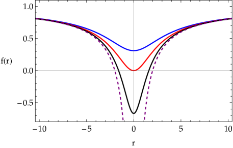
Figure 1: The $f(r)$ metric function of the Simpson-Visser geometry (27) corresponding to a traversable wormhole (blue curve, for $p\equiv\alpha/m=2.9$), an extremal regular BH (red curve, for $p=2$), a black bounce (black curve, for $p=1.2$), the Schwarzschild BH limit (dashed curve, for $p\to 0$).

Notice that the metric (27) is not in the Morris-Thorne frame (4) since $K^{2}(r)\neq r^{2}$. To this end, one may perform the coordinate transformation $r\rightarrow\tilde{r}:\tilde{r}^{2}=r^{2}+\alpha^{2}\,,$ in order to recast the metric to the MT frame where it is written as

$$ds^{2}=-\left(1-\frac{2\,m}{\tilde{r}}\right)dt^{2}+\left(1-\frac{2\,m}{\tilde{r}}\right)^{-1}\left(1-\frac{\alpha^{2}}{\tilde{r}^{2}}\right)^{-1}d\tilde{r}^{2}+\tilde{r}^{2}d\Omega^{2}\,.$$ (28)

Then, one may proceed with the parametrization in terms of (11) and (17). The condition (5), that determines the location of the WH throat $r_{0}$ in the MT frame, yields the following equation in the case of the SV wormhole

$$h(r)\equiv\left(1-\frac{2\,m}{\tilde{r}}\right)\left(1-\frac{\alpha^{2}}{\tilde{r}^{2}}\right)=0\,.$$ (29)

There are two roots to the above equation, which are located at $\tilde{r}=2m$ and $\tilde{r}=\alpha$. The former root, is not a suitable choice for a WH throat because in this case $f(\tilde{r}_{0})=0$, and an event horizon emerges. Thus, the WH branch corresponds to the region in the parametric space defined by $\alpha>2m$. Since the metric functions in (28) are of polynomial form, the parametrization is exact with the EPs given by

$$\epsilon = \frac{2m}{\alpha}-1\,,\quad a_{0}=0\,,\quad f_{0}=1-\frac{2m}{\alpha}\,,\quad a_{i}=0\quad\forall i\geqslant 1\,,$$

$$b_{0} = \frac{2m}{\alpha}-1\,,\quad h_{0}=0\,,\quad b_{1}=-\frac{2m}{\alpha}\,,\quad b_{i}=0\quad\forall i\geqslant 2\,.$$ (30)

A general parametrization for WH metrics in non-MT frames by means of (16) and (17), is also possible upon appropriate modification of the DCC. In particular, for the line-element (27), the optimized version of the DCC

$$x(r)=1-\sqrt{\frac{R_{0}^{2}}{R_{0}^{2}+r^{2}}}\,,\qquad R_{0}=\alpha\sqrt{\frac{3}{2}}\,,$$ (31)

yields a parametrization for the SV metric with the first few EPs given by

$$\epsilon = \frac{2m}{R_{0}}-1\,,\quad a_{0}=0\,,\quad f_{0}=1-\frac{2m}{\alpha}\,,\quad a_{1}=2\epsilon+3f_{0}-1+\frac{2mR_{0}^{2}}{\alpha^{3}}\,,$$

$$a_{2} = \frac{3}{2a_{1}}\left(4\epsilon+5f_{0}-3a_{1}-1+\frac{2mR_{0}^{4}}{\alpha^{5}}\right)\,.$$ (32)

5 Shadows and perturbations of test fields

In this section, as gauge-invariant tests for the accuracy of the parametrization, we consider shadows and perturbations of test fields in the background of the approximate WH metrics obtained by considering various orders in the continued-fraction expansion and compare them with the corresponding values obtained when the exact metric expressions are used.

5.1 Shadows of the anti-Fisher wormhole

In the context of GR with a massless minimally-coupled scalar field, a solution containing a naked singularity has been found Fisher (1948). When the kinetic term of the scalar field has the opposite sign, a solution emerges which has a WH branch and has been called anti-Fisher solution Bronnikov (1973). The metric functions for the latter solution assume the following form

$$f(r)=h(r)=e^{2u(r)}\,,\quad K^{2}(r)=e^{-2u(r)}\left(r^{2}+\alpha^{2}\right)\,,\quad u(r)\equiv\frac{m}{\alpha}\left(\arctan\frac{r}{\alpha}-\frac{\pi}{2}\right)\,.$$ (33)

Substitution of (33) in the general expression (10), yields the shadow radius for the anti-Fisher WH

$$R_{\rm sh}=e^{-2\,u(r_{\rm ph})}\sqrt{4m^{2}+\alpha^{2}}\,,$$ (34)

where $r_{\rm ph}=2m$ is the photon sphere radius which has been determined via (7). The first few EPs for the parametrization of $f(r)$ in this case are given by

$$\epsilon = 1\,,\quad a_{0}=2\,,\quad f_{0}=e^{2u(m)}\,,\quad a_{1}=f_{0}\left(3+\frac{2m^{2}}{\alpha^{2}+m^{2}}\right)-1\,,$$

$$a_{2} = \frac{6f_{0}-4a_{1}-2}{a_{1}}\,,\quad a_{3}=-\frac{f_{0}\left[\frac{2m^{4}}{3\left(\alpha^{2}+m^{2}\right)^{2}}-10\right]+a_{1}\left[10+a_{2}\left(5+a_{2}\right)\right]+4}{a_{1}a_{2}}\,.$$ (35)

By considering various orders in the approximation of $f(r)$ via (16) and (35), we once again compute the shadow radius by means of (10) and compare the result order-by-order with the exact value given in Eq. (34). Our findings Bronnikov et al. (2021) are presented in terms of the dimensionless parameter $p\equiv\alpha/m$ in Table 2. The high accuracy of the approximation already at the first order and the quick convergence are evident.

Table 2: The percentage of absolute relative error between the exact value of the shadow radius (34) and its value as obtained via Eq. (10) for various approximation orders of the metric function $f(r)$.

order	$p=0.01$	$p=0.2$	$p=0.3$	$p=0.4$	$p=0.5$	$p=0.6$
1	1.04775	0.95530	0.83863	0.67406	0.46096	0.19918
2	0.02753	0.03339	0.04295	0.06093	0.09281	0.14633
3	0.00304	0.00387	0.00570	0.01061	0.02367	0.05883
4	0.00011	0.00019	0.00034	0.00063	0.00112	0.00186

5.2 Shadows of the Simpson-Visser wormhole

As a second example for shadows in a wormhole background we consider the SV metric in the non-Morris-Thorne frame i.e. (27), for which we obtain the exact expression for the shadow radius

$$R_{\rm sh}=3\sqrt{3}m\,.$$ (36)

Notice that value of $R_{\rm sh}$ is independent of the parameter $\alpha$ and it is identified with the shadow radius of the Schwarzschild BH, for detailed discussions see Tsukamoto (2021); Lima et al. (2021). Subsequently, by considering various orders for the approximate metric according to (32), we compute once again $R_{\rm sh}$ and compare it with the exact result (36). The range of values for the dimensionless parameter $p\equiv\alpha/m$ that is relevant for the analysis here is $p\in[2,3]$ where the lower bound corresponds to the WH/BH threshold and the upper bound corresponds to the maximum value of $p$ for which the spacetime under consideration exhibits a photon sphere. Our findings Bronnikov et al. (2021) are displayed in Table 3.

Table 3: The percentage of absolute relative error between the analytic value of the shadow and its value for various approximation orders of the metric.

order	$p=2.01$	$p=2.1$	$p=2.4$	$p=2.5$	$p=2.7$	$p=2.99$
1	0.54727	0.47968	0.25291	0.18463	0.07285	0.00009
2	0.01973	0.01568	0.00544	0.00329	0.00076	$\mathcal{O}(10^{-8})$
3	0.00278	0.00200	0.00046	0.00023	0.00003	$\mathcal{O}(10^{-11})$
4	0.00060	0.00039	0.00005	0.00002	$\mathcal{O}(10^{-6})$	$\mathcal{O}(10^{-13})$

We observe that already with the first-order approximation of the metric, the error is less than $1\%$ for all values of $p$, and it is monotonically decreasing from the WH/BH threshold all the way to the no-photon sphere limit. Furthermore, one can see the quick convergence of the series where the error is reduced by approximately one order of magnitude with each additional term in the expansion that is taken into account.

5.3 Quasinormal modes

Let us now consider the fundamental quasinormal modes (QNMs) of the electromagnetic field propagating in a WH background. QNMs are characteristic frequencies of a compact object which are independent of the initial conditions of perturbations and are completely determined by the parameters of the compact object under consideration Kokkotas and Schmidt (1999); Berti et al. (2009); Konoplya and Zhidenko (2011). The real part of a QNM represents a real oscillation frequency, while the imaginary part is proportional to the damping rate. For a non exhaustive list of works where QNMs in WHs backgrounds have been studied, see Konoplya and Zhidenko (2010); Bronnikov et al. (2012); Taylor (2014); Cuyubamba et al. (2018); VĂślkel and Kokkotas (2018); Aneesh et al. (2018); Konoplya (2018); Kim et al. (2018); Dutta Roy et al. (2020); Churilova et al. (2020); Jusufi (2021); Biswas et al. (2022). An electromagnetic field obeys the general covariant Maxwell equations

$$\dfrac{1}{\sqrt{-g}}\partial_{\mu}\left(F_{\rho\sigma}g^{\rho\nu}g^{\sigma\mu}\sqrt{-g}\right)=0.$$ (37)

Here $F_{\rho\sigma}=\partial_{\rho}A_{\sigma}-\partial_{\sigma}A_{\rho}$ and $A_{\mu}$ is a vector potential. For the spherically-symmetric spacetime (1), one may introduce the “tortoise coordinate” $r_{*}$, in terms of the metric functions $f(r)$ and $h(r)$ as

$$dr_{*}=\frac{dr}{\sqrt{f(r)h(r)}}\,.$$ (38)

Then, after separation of variables, Eq. (37) assumes the following wave-like form

$$\dfrac{d^{2}\Psi}{dr_{*}^{2}}+\left(\omega^{2}-V(r)\right)\Psi=0\,,$$ (39)

and the effective potential reads as

$$V_{\rm em}(r)=f(r)\frac{\ell(\ell+1)}{r^{2}}\,.$$ (40)

Even though the effective potential depends on the gravitational background only via the metric function $f(r)$, the QNMs will depend on both $f(r)$ and $h(r)$ implicitly via the tortoise coordinate (38). The boundary conditions for finding QNMs in a WH background correspond to purely outgoing waves at both infinities $r_{*}\rightarrow\pm\infty\,$ Konoplya and Molina (2005). The values of QNMs obtained for the Bronnikov-Kim II and Simpson-Viser WHs both of which have been discussed in the previous sections are displayed in Tables 4 and 5 respectively Bronnikov et al. (2021).

Table 4: Fundamental quasinormal modes ($\ell=1$, $n=0$) of the electromagnetic field for the Bronnikov-Kim II wormhole.

order	$C=-0.01$	$C=-0.3$	$C=-0.7$
exact	$0.64306-0.20529i$	$0.70322-0.03991i$	$0.73338-0.09961i$
$1$st	$0.65899-0.19306i$	$0.70232-0.03741i$	$0.73304-0.09836i$
$2$nd	$0.64093-0.20593i$	$0.70332-0.04009i$	$0.73345-0.09969i$

Table 5: Fundamental quasinormal modes ($\ell=1$, $n=0$) of the electromagnetic field for the Simpson-Visser wormhole ($m=1/2$).

order	$\alpha=1.01$	$\alpha=1.25$	$\alpha=1.4$
exact	$0.51125-0.13311i$	$0.55491-0.03299i$	$0.56858-0.05986i$
$1$st	$0.50899-0.13211i$	$0.55394-0.03297i$	$0.56770-0.05982i$
$2$nd	$0.51241-0.13405i$	$0.55520-0.03286i$	$0.56885-0.05969i$

As it can be seen, the QNMs obtained with the first two orders in the continued-fraction expansion of the background metric approximate very accurately the values obtained in terms of the exact metric.

6 Conclusions

Building upon the Rezzolla and Zhidenko (2014) theory-agnostic parametrization of BH spacetimes, we have introduced an extension that allows for general Lorentzian, traversable, static and asymptotically-flat WH metrics to be accommodated in this parameterized framework Bronnikov et al. (2021). The parametrization is based on a continued-fraction expansion in terms of a compactified radial coordinate, exhibits rapid convergence properties, and is valid in all of spacetime.

We have obtained the parametrizations for various examples of known wormhole geometries and studied the shadows and perturbations of test fields in these gravitational backgrounds for different orders in the expansion. Quite importantly, by considering geometries that interpolate continuously between a BH and a WH, we have demonstrated that the parametrization is very accurate, (already at the first and in some cases second-order in the expansion), even at the WH/BH threshold and this is relevant for WHs that act as BH mimickers.

Our analysis demonstrates that when a WH metric changes relatively slowly in the radiation zone, the observable effects in the wormhole background depend only on a few parameters and the following approximation for the line-element is sufficient Bronnikov et al. (2021)

$$ds^{2} = -f(r)dt^{2}+\frac{1}{h(r)}dr^{2}+r^{2}d\Omega^{2}\,,$$ (41)

$$f(r) = 1-\frac{r_{0}\left(1+\epsilon\right)}{r}+\frac{r_{0}^{3}\left(a_{1}+f_{0}+\epsilon\right)}{r^{3}}-\frac{r_{0}^{4}\,a_{1}}{r^{4}}\,,$$ (42)

$$h(r) = 1-\frac{r_{0}\left(1+\epsilon\right)}{r}+\frac{r_{0}^{2}\left(b_{1}+h_{0}+\epsilon\right)}{r^{2}}-\frac{r_{0}^{3}\,b_{1}}{r^{3}}\,.$$ (43)

References

- Aneesh et al. (2018) Aneesh, S., Bose, S. and Kar, S. (2018), Gravitational waves from quasinormal modes of a class of Lorentzian wormholes, Phys. Rev., D97(12), p. 124004, 1803.10204.
- Bambi and Stojkovic (2021) Bambi, C. and Stojkovic, D. (2021), Astrophysical Wormholes, Universe, 7(5), p. 136, 2105.00881.
- Berti et al. (2009) Berti, E., Cardoso, V. and Starinets, A. O. (2009), Quasinormal modes of black holes and black branes, Class. Quant. Grav., 26, p. 163001, 0905.2975.
- Biswas et al. (2022) Biswas, S., Rahman, M. and Chakraborty, S. (2022), Echoes from braneworld wormholes, Phys. Rev. D, 106(12), p. 124003, 2205.14743.
- Blázquez-Salcedo et al. (2021) Blázquez-Salcedo, J. L., Knoll, C. and Radu, E. (2021), Traversable wormholes in Einstein-Dirac-Maxwell theory, Phys. Rev. Lett., 126(10), p. 101102, 2010.07317.
- Bolokhov et al. (2021) Bolokhov, S., Bronnikov, K., Krasnikov, S. and Skvortsova, M. (2021), A Note on “Traversable Wormholes in Einstein–Dirac–Maxwell Theory”, Grav. Cosmol., 27(4), pp. 401–402, 2104.10933.
- Bolokhov et al. (2012) Bolokhov, S. V., Bronnikov, K. A. and Skvortsova, M. V. (2012), Magnetic black universes and wormholes with a phantom scalar, Class. Quant. Grav., 29, p. 245006, 1208.4619.
- Bronnikov and Kim (2003) Bronnikov, K. and Kim, S.-W. (2003), Possible wormholes in a brane world, Phys. Rev. D, 67, p. 064027, gr-qc/0212112.
- Bronnikov (1973) Bronnikov, K. A. (1973), Scalar-tensor theory and scalar charge, Acta Phys. Polon. B, 4, pp. 251–266.
- Bronnikov (2018) Bronnikov, K. A. (2018), Scalar fields as sources for wormholes and regular black holes, Particles, 1(1), pp. 56–81, 1802.00098.
- Bronnikov and Fabris (2006) Bronnikov, K. A. and Fabris, J. C. (2006), Regular phantom black holes, Phys. Rev. Lett., 96, p. 251101, gr-qc/0511109.
- Bronnikov et al. (2011) Bronnikov, K. A., Fabris, J. C. and Zhidenko, A. (2011), On the stability of scalar-vacuum space-times, Eur. Phys. J. C, 71, p. 1791, 1109.6576.
- Bronnikov and Grinyok (2001) Bronnikov, K. A. and Grinyok, S. (2001), Instability of wormholes with a nonminimally coupled scalar field, Grav. Cosmol., 7, pp. 297–300, gr-qc/0201083.
- Bronnikov and Konoplya (2020) Bronnikov, K. A. and Konoplya, R. A. (2020), Echoes in brane worlds: ringing at a black hole–wormhole transition, Phys. Rev. D, 101(6), p. 064004, 1912.05315.
- Bronnikov et al. (2021) Bronnikov, K. A., Konoplya, R. A. and Pappas, T. D. (2021), General parametrization of wormhole spacetimes and its application to shadows and quasinormal modes, Phys. Rev. D, 103(12), p. 124062, 2102.10679.
- Bronnikov et al. (2012) Bronnikov, K. A., Konoplya, R. A. and Zhidenko, A. (2012), Instabilities of wormholes and regular black holes supported by a phantom scalar field, Phys. Rev., D86, p. 024028, 1205.2224.
- Bronnikov et al. (2007) Bronnikov, K. A., Melnikov, V. N. and Dehnen, H. (2007), Regular black holes and black universes, Gen. Rel. Grav., 39, pp. 973–987, gr-qc/0611022.
- Bronnikov and Walia (2022) Bronnikov, K. A. and Walia, R. K. (2022), Field sources for Simpson-Visser spacetimes, Phys. Rev. D, 105(4), p. 044039, 2112.13198.
- Churilova et al. (2020) Churilova, M. S., Konoplya, R. A. and Zhidenko, A. (2020), Arbitrarily long-lived quasinormal modes in a wormhole background, Phys. Lett., B802, p. 135207, 1911.05246.
- Churilova and Stuchlik (2020) Churilova, M. S. and Stuchlik, Z. (2020), Ringing of the regular black-hole/wormhole transition, Class. Quant. Grav., 37(7), p. 075014, 1911.11823.
- Cuyubamba et al. (2018) Cuyubamba, M. A., Konoplya, R. A. and Zhidenko, A. (2018), No stable wormholes in Einstein-dilaton-Gauss-Bonnet theory, Phys. Rev., D98(4), p. 044040, 1804.11170.
- Damour and Solodukhin (2007) Damour, T. and Solodukhin, S. N. (2007), Wormholes as black hole foils, Phys. Rev., D76, p. 024016, 0704.2667.
- Dutta Roy et al. (2020) Dutta Roy, P., Aneesh, S. and Kar, S. (2020), Revisiting a family of wormholes: geometry, matter, scalar quasinormal modes and echoes, Eur. Phys. J., C80(9), p. 850, 1910.08746.
- Einstein and Rosen (1935) Einstein, A. and Rosen, N. (1935), The Particle Problem in the General Theory of Relativity, Phys. Rev., 48, pp. 73–77.
- Ellis (1973) Ellis, H. G. (1973), Ether flow through a drainhole - a particle model in general relativity, J. Math. Phys., 14, pp. 104–118.
- Fisher (1948) Fisher, I. Z. (1948), Scalar mesostatic field with regard for gravitational effects, Zh. Eksp. Teor. Fiz., 18, pp. 636–640, gr-qc/9911008.
- Flamm (1916) Flamm, L. (1916), Beiträge zur Einsteinschen Gravitationstheorie, Phys. Z., 17, p. 448.
- Gonzalez et al. (2009) Gonzalez, J. A., Guzman, F. S. and Sarbach, O. (2009), Instability of wormholes supported by a ghost scalar field. I. Linear stability analysis, Class. Quant. Grav., 26, p. 015010, 0806.0608.
- Hennigar et al. (2018) Hennigar, R. A., Poshteh, M. B. J. and Mann, R. B. (2018), Shadows, Signals, and Stability in Einsteinian Cubic Gravity, Phys. Rev. D, 97(6), p. 064041, 1801.03223.
- Jusufi (2021) Jusufi, K. (2021), Correspondence between quasinormal modes and the shadow radius in a wormhole spacetime, Gen. Rel. Grav., 53(9), p. 87, 2007.16019.
- Kim et al. (2018) Kim, J. Y., Lee, C. O. and Park, M.-I. (2018), Quasi-Normal Modes of a Natural AdS Wormhole in Einstein-Born-Infeld Gravity, Eur. Phys. J., C78(12), p. 990, 1808.03748.
- Kokkotas et al. (2017) Kokkotas, K., Konoplya, R. A. and Zhidenko, A. (2017), Non-Schwarzschild black-hole metric in four dimensional higher derivative gravity: analytical approximation, Phys. Rev. D, 96, p. 064007, 1705.09875.
- Kokkotas and Schmidt (1999) Kokkotas, K. D. and Schmidt, B. G. (1999), Quasinormal modes of stars and black holes, Living Rev. Rel., 2, p. 2, gr-qc/9909058.
- Konoplya et al. (2016) Konoplya, R., Rezzolla, L. and Zhidenko, A. (2016), General parametrization of axisymmetric black holes in metric theories of gravity, Phys. Rev., D93(6), p. 064015, 1602.02378.
- Konoplya and Zhidenko (2010) Konoplya, R. and Zhidenko, A. (2010), Passage of radiation through wormholes of arbitrary shape, Phys. Rev. D, 81, p. 124036, 1004.1284.
- Konoplya (2018) Konoplya, R. A. (2018), How to tell the shape of a wormhole by its quasinormal modes, Phys. Lett., B784, pp. 43–49, 1805.04718.
- Konoplya and Molina (2005) Konoplya, R. A. and Molina, C. (2005), The Ringing wormholes, Phys. Rev., D71, p. 124009, gr-qc/0504139.
- Konoplya et al. (2020a) Konoplya, R. A., Pappas, T. and Zhidenko, A. (2020a), Einstein-scalar–Gauss-Bonnet black holes: Analytical approximation for the metric and applications to calculations of shadows, Phys. Rev. D, 101(4), p. 044054, 1907.10112.
- Konoplya et al. (2020b) Konoplya, R. A., Pappas, T. D. and Stuchlík, Z. (2020b), General parametrization of higher-dimensional black holes and its application to Einstein-Lovelock theory, Phys. Rev. D, 102(8), p. 084043, 2007.14860.
- Konoplya and Zhidenko (2011) Konoplya, R. A. and Zhidenko, A. (2011), Quasinormal modes of black holes: From astrophysics to string theory, Rev. Mod. Phys., 83, pp. 793–836, 1102.4014.
- Konoplya and Zhidenko (2019) Konoplya, R. A. and Zhidenko, A. (2019), Analytical representation for metrics of scalarized Einstein-Maxwell black holes and their shadows, Phys. Rev. D, 100(4), p. 044015, 1907.05551.
- Konoplya and Zhidenko (2022a) Konoplya, R. A. and Zhidenko, A. (2022a), How general is the strong cosmic censorship bound for quasinormal modes?, JCAP, 11, p. 028, 2210.04314.
- Konoplya and Zhidenko (2022b) Konoplya, R. A. and Zhidenko, A. (2022b), Traversable Wormholes in General Relativity, Phys. Rev. Lett., 128(9), p. 091104, 2106.05034.
- Konoplya and Zhidenko (2023) Konoplya, R. A. and Zhidenko, A. (2023), Overtones’ outburst of asymptotically AdS black holes, 2310.19205.
- Lima et al. (2021) Lima, H. C. D., Junior., Crispino, L. C. B., Cunha, P. V. P. and Herdeiro, C. A. R. (2021), Can different black holes cast the same shadow?, Phys. Rev. D, 103(8), p. 084040, 2102.07034.
- Mazza et al. (2021) Mazza, J., Franzin, E. and Liberati, S. (2021), A novel family of rotating black hole mimickers, JCAP, 04, p. 082, 2102.01105.
- Morris and Thorne (1988) Morris, M. S. and Thorne, K. S. (1988), Wormholes in space-time and their use for interstellar travel: A tool for teaching general relativity, Am. J. Phys., 56, pp. 395–412.
- Perlick et al. (2015) Perlick, V., Tsupko, O. Y. and Bisnovatyi-Kogan, G. S. (2015), Influence of a plasma on the shadow of a spherically symmetric black hole, Phys. Rev. D, 92(10), p. 104031, 1507.04217.
- Randall and Sundrum (1999) Randall, L. and Sundrum, R. (1999), An Alternative to compactification, Phys. Rev. Lett., 83, pp. 4690–4693, hep-th/9906064.
- Rezzolla and Zhidenko (2014) Rezzolla, L. and Zhidenko, A. (2014), New parametrization for spherically symmetric black holes in metric theories of gravity, Phys. Rev. D, 90(8), p. 084009, 1407.3086.
- Shiromizu et al. (2000) Shiromizu, T., Maeda, K.-i. and Sasaki, M. (2000), The Einstein equation on the 3-brane world, Phys. Rev., D62, p. 024012, gr-qc/9910076.
- Simpson and Visser (2019) Simpson, A. and Visser, M. (2019), Black-bounce to traversable wormhole, JCAP, 02, p. 042, 1812.07114.
- Synge (1966) Synge, J. L. (1966), The Escape of Photons from Gravitationally Intense Stars, Mon. Not. Roy. Astron. Soc., 131(3), pp. 463–466.
- Taylor (2014) Taylor, P. (2014), Propagation of Test Particles and Scalar Fields on a Class of Wormhole Space-Times, Phys. Rev., D90(2), p. 024057, [Erratum: Phys. Rev.D95,no.10,109904(2017)], 1404.7210.
- Tsukamoto (2021) Tsukamoto, N. (2021), Gravitational lensing in the Simpson-Visser black-bounce spacetime in a strong deflection limit, Phys. Rev. D, 103(2), p. 024033, 2011.03932.
- Visser (1995) Visser, M. (1995), Lorentzian wormholes: From Einstein to Hawking, ISBN 978-1-56396-653-8.
- VĂślkel and Kokkotas (2018) VĂślkel, S. H. and Kokkotas, K. D. (2018), Wormhole Potentials and Throats from Quasi-Normal Modes, Class. Quant. Grav., 35(10), p. 105018, 1802.08525.
- Wheeler (1955) Wheeler, J. A. (1955), Geons, Phys. Rev., 97, pp. 511–536.
- Will (2006) Will, C. M. (2006), The Confrontation between general relativity and experiment, Living Rev. Rel., 9, p. 3, gr-qc/0510072.
- Will (2014) Will, C. M. (2014), The Confrontation between General Relativity and Experiment, Living Rev. Rel., 17, p. 4, 1403.7377.
- Younsi et al. (2016) Younsi, Z., Zhidenko, A., Rezzolla, L., Konoplya, R. and Mizuno, Y. (2016), New method for shadow calculations: Application to parametrized axisymmetric black holes, Phys. Rev. D, 94(8), p. 084025, 1607.05767.