Gravitational waves from quasinormal modes of a class of Lorentzian wormholes

Abstract

Quasinormal modes of a two-parameter family of Lorentzian wormhole spacetimes, which arise as solutions in a specific scalar-tensor theory associated with braneworld gravity, are obtained using standard numerical methods. Being solutions in a scalar-tensor theory, these wormholes can exist with matter satisfying the Weak Energy Condition. If one posits that the end-state of stellar-mass binary black hole mergers, of the type observed in GW150914, can be these wormholes, then we show how their properties can be measured from their distinct signatures in the gravitational waves emitted by them as they settle down in the post-merger phase from an initially perturbed state. We propose that their scalar quasinormal modes correspond to the so-called breathing modes, which normally arise in gravitational wave solutions in scalar-tensor theories. We show how the frequency and damping time of these modes depend on the wormhole parameters, including its mass. We derive the mode solutions and use them to determine how one can measure those parameters when these wormholes are the endstate of binary black hole mergers. Specifically, we find that if a breathing mode is observed in LIGO-like detectors with design sensitivity, and has a maximum amplitude equal to that of the tensor mode that was observed of GW150914, then for a range of values of the wormhole parameters, we will be able to discern it from a black hole. If in future observations we are able to confirm the existence of such wormholes, we would, at one go, have some indirect evidence of a modified theory of gravity as well as extra spatial dimensions.

I Introduction

Lorentzian wormholes have been around as theoretical constructs ever since the idea of the Einstein-Rosen (ER) bridge was born in 1935 einstein . Among many of Einstein’s ideas and predictions, gravitational waves (GW) and the cosmological constant are a part of reality today gwobs ; gwobs1 ; lambda , but the Einstein-Rosen bridge and its progeny – the wormholes– are yet to see the light of day in the real universe.

Subsequent to the ER article and about a couple of decades later, Misner and Wheeler, in their paper on classical physics as geometry mw , first introduced the term wormhole. Later, through the work of Ellis ellis , Bronnikov bronnikov , Morris, Thorne and Yurtsever mty , Morris and Thorne mt , Novikov novikov , Novikov and Frolov novikov1 , Visser visser and many others wothers1 ; wothers2 ; wothers3 ; wothers4 ; wothers5 ; wothers6 ; wothers7 ; wothers8 ; wothers9 ; wothers10 ; wothers11 , the wormhole idea was further developed with numerous examples as well as enquiries into the intriguing possibilities that may arise with wormholes (eg. time machines! mty ; novikov ; novikov1 ). Even today, the term wormhole, does appear almost every day, in one article or the other, in the daily list of submitted articles in preprint archives.

Wormholes are, in some sense, good spacetimes! They do not have horizons or singularities, which make things interesting as well as difficult. But the absence of horizons or singularities for wormholes comes at a heavy cost. The matter required to have a wormhole violates the so-called energy conditions hawkellis ; wald , atleast in the context of General Relativity. Wormholes seem to require exotic matter – i.e., matter for which energy density can become negative in some frame of reference.

Is there a way to avoid this impasse? Many resolutions have been suggested in the past wecviolation1 ; wecviolation2 ; wecviolation3 ; hochberg ; wecviolation4 ; wecviolation5 ; roman ; wecviolation6 ; wecviolation7 ; wecviolation8 ; wecviolation9 ; wecviolation10 ; canfora1 ; canfora2 Among them, one avenue is to look into modified theories of gravity where additional degrees of freedom (e.g., say a scalar field) have a role to play. In the old Brans-Dicke idea bransdicke ; bransdicke1 , the scalar field replaced the gravitational constant $G$. In later versions and the most recent ones, the scalar field can actually arise via the presence of extra spatial dimensions kannosoda . A well-known model that exploits this is the on-brane gravity kannosoda arising in the so-called two-brane model of Randall–Sundrum randall , wherein the scalar field is related to the inter-brane-distance. Thus, we and our wormhole would be on one such 3-brane and a scalar field, which is not quite ‘matter’, would provide the required negativity so that the ‘convergence condition’ is violated (as it must be for wormholes) hawkellis , but the ‘matter’ threading the wormhole is usual matter, with all the desired properties. The above line of thought was exploited to construct a class of wormholes with matter satisfying the energy conditions, in work done recently by one of the authors here (along with others)sksl ; sksl1 . In a way, therefore, the existence of the wormhole would therefore provide support to an alternative theory of gravity, as well as to the existence of extra dimensions!

How then does one show that such a wormhole does indeed exist? Motivated by recent detections of gravitational waves at LIGO and Virgo gwobs ; gwobs1 , we explore whether there is any meaning to a proposal that the final state of some violent collision of neutron stars and/or black holes might result in a wormhole of the type we mention above or, more, realistically, its rotating version. We do not have any model which shows that a wormhole may indeed emerge in such a collision. However, such a suggestion is not entirely new. (See ringdown1 ; damour ; taylor ; ringdown2 ; ringdown3 ; echoes ; rezzolla for earlier work as well a more recent one on GW signals from wormholes.) All we can say, is that, by studying the ringdown and the quasinormal modes (which we find here), we can, through a comparison with observational data, estimate the error bounds in the parameters which define the wormhole and appear in the quasi-normal modes. The values of the wormhole parameters may be constrained by other means such as lensing or time-delay. Thereafter, we can say, to what extent, through gravitational wave observations we can constrain the merged object to be a wormhole. It is true, however, that the BBH (binary black hole) GW signals observed so far are all consistent with the merger of two Kerr black holes to another Kerr black hole, but the extent to which mergers of objects that are not Kerr black holes could resemble these signals is yet to be established [2,3].

Our paper is organised as follows. In the next section, we briefly recall the spacetime and the theory for which this is a solution. Thereafter, in Section III, we set up the search for massless scalar quasinormal modes, in this background geometry. We try to justify how these scalar QNMs could precisely be those for the so-called breathing mode. We solve for QNMs numerically, find them and demonstrate their characteristics through various plots and analysis. In Section IV, we demonstrate how one can estimate the errors in the wormhole parameters (more precisely, one parameter) using inputs from GW observations. Finally, in Section V, we sum up and provide possible avenues for future work. In the rest of the paper we will use units in which $G=1$ and $c=1$.

II The class of wormhole spacetimes

Let us begin with the modified theory of gravity, in which, our wormhole is a solution. As stated in the Introduction, this is a scalar-tensor theory of a specific type. It arises as a theory on the four dimensional 3-brane timelike hypersurface in a five-dimensional background. We have two 3-branes separated by a distance in extra-dimensional space– the inter-brane distance is associated with the scalar, in our low-energy, effective, on-brane scalar tensor theory of gravity. The subsections below briefly recall the theory as well as the wormhole solution.

II.1 Scalar tensor gravity, field equations, wormhole solutions

The field equations for the on-brane scalar-tensor theory of gravity are given by kannosoda ,

$$R_{\mu\nu}=\frac{\bar{\kappa}}{l\Phi}\left(T^{b}_{\mu\nu}-\frac{1}{2}g_{\mu\nu}T^{b}\right)+\frac{\Omega(\Phi)}{\Phi^{2}}\nabla_{\mu}\Phi\nabla_{\nu}\Phi+\frac{1}{\Phi}\left(\nabla_{\mu}\nabla_{\nu}\Phi+\frac{1}{2}g_{\mu\nu}\Box\Phi\right)$$ (1)

where $T^{b}_{\mu\nu}$ is the stress energy tensor on the 3-brane (labeled as the “$b$” brane in kannosoda ) and $\Phi$ is the scalar field which satisfies the field equation,

$$\Box\Phi=\frac{\bar{\kappa}}{l}\frac{T^{b}}{2\Omega+3}-\frac{1}{2\Omega+3}\frac{d\Omega}{d\Phi}\nabla^{\alpha}\Phi\nabla_{\alpha}\Phi$$ (2)

$l$ is the bulk curvature radius and $\bar{\kappa}$ is related to the higher dimensional Newton constant. The coupling function $\Omega(\Phi)$ can be expressed in terms of the scalar field as,

$$\Omega(\Phi)=-\frac{3\Phi}{2(1+\Phi)}$$ (3)

The scalar field $\Phi$, as mentioned before, is associated with the inter-brane distance in the bulk. It has to be non-zero, positive and finite in order to have a meaningful two-brane model. $T^{b}$ is the trace of the stress-energy on the “$b$” 3-brane, embedded in a five dimensional bulk spacetime. The above field equations are for the scalar-tensor theory on this so-called $b$-brane. For more details about the theory, the reader is referred to kannosoda .

In the above-mentioned theory, we now consider a static, spherically symmetric wormhole solution of the field equations with a vanishing Ricci scalar. Such a solution has been shown to be given by sksl (see earlier work in R3 ; R3' ),

$$ds^{2}=-\left(\kappa+\lambda\sqrt{1-\frac{2M}{r}}\right)^{2}dt^{2}+\frac{dr^{2}}{1-\frac{2M}{r}}+r^{2}\left(d\theta^{2}+\sin^{2}\theta d\phi^{2}\right)$$ (4)

where $\kappa$, $\lambda$ are non-zero, positive constants. Note that our wormhole has two parameters: $M$, a measure of the throat radius ($2M$ here, like in Schwarzschild) and $\frac{\kappa}{\lambda}>0$ which, being non-zero, signals the absence of a horizon.

The Jordan frame scalar field $\Phi$ takes the form,

$$\Phi=\left(\frac{c_{1}}{M\lambda}\ln\frac{2r^{\prime}q+M}{2r^{\prime}+M}+c_{2}\right)^{2}-1$$ (5)

where $r=r^{\prime}(1+\frac{m}{2r^{\prime}})^{2}$ ($r^{\prime}$ is the isotropic coordinate), $q=\frac{\kappa+\lambda}{\kappa-\lambda}>1$ and $c_{1}$, $c_{2}$ are constants of integration, in this solution. Assuming $c_{2}=0$ one can show that the WEC can hold under specific choices of the various parameters sksl . Note that the timelike or null convergence condition is indeed violated, as it should be, in order to ensure that the spacetime is a wormhole. However, the required matter satisfies the WEC. For more details about the solution, the stress-energy of the matter that supports the wormhole, as well as the WEC see sksl .

If $q<0$ (i.e. $\frac{\kappa}{\lambda}<1$), the scalar field solution remains similar in its functional form. In order to have a finite, non-zero radion scalar and also ensure that the WEC holds, we need $c_{2}\neq 0$, as well as additional constraints on the parameters.

II.2 Scalar field propagation

How does a massless scalar field (not necessarily the scalar $\Phi$ in the theory mentioned above, but any generic scalar field) propagate in the above-mentioned background spacetime? Such a scalar field, as we show later, is related to the perturbations of the Brans-Dicke scalar $\Phi$, which we introduced in the previous subsection. In addition, there are also gravitational perturbations which we do not fully consider here. Our problem therefore reduces to solving a massless Klein-Gordon equation in a fixed, curved background, i.e.

$$\Box\Psi=0$$ (6)

Since the background spacetime is spherically symmetric and static, we can decompose $\Psi$ in terms of the spherical harmonics,

$$\Psi(t,r,\theta,\phi)=\sum_{l=0}^{\infty}\sum_{m=-l}^{l}\frac{\psi_{lm}(r)}{r}e^{-i\omega t}Y_{lm}(\theta,\phi)$$ (7)

By inserting this ansatz in the Klein-Gordon equation we get the equation satisfied by each mode,

$$fh\frac{d^{2}\psi_{lm}}{dr^{2}}+\frac{1}{2}(hf^{\prime}+fh^{\prime})\frac{d\psi_{lm}}{dr}+\omega^{2}\psi_{lm}=\frac{rhf^{\prime}+f(2l(l+1)+rh^{\prime})}{2r^{2}}\psi_{lm}$$ (8)

where have defined $f(r)=-g_{tt}$ and $h(r)=(g_{rr})^{-1}$. We can rewrite the above equation by introducing the tortoise coordinate $r_{*}$ defined as,

$$\frac{dr_{*}}{dr} =(fh)^{-1/2}$$ (9)

The above equation can be integrated to obtain an analytical expression for the tortoise coordinate, given as,

$$r_{*}=\frac{M}{\lambda}\left\{\frac{2(p-\beta)(2p-\beta)}{(p^{2}-1)\left[(p-\beta)^{2}-1\right]}+4\frac{\ln\frac{\beta}{p}}{(p^{2}-1)^{2}}+\frac{(p-2)\ln(1-p+\beta)}{(p-1)^{2}}-\frac{(2+p)\ln(1+p-\beta)}{(1+p)^{2}}\right\}$$ (10)

where $p=\frac{\kappa}{\lambda}$, $\beta=p+\sqrt{1-\frac{2M}{r}}$. The asymptotic regions of the wormhole correspond to $r_{*}\rightarrow\pm\infty$. We need to use $\pm r_{*}$ in order to cover the two asymptotic regions connected by the throat, which requires a thin shell joining two copies of the same geometry visser . In some sense, $r_{*}$ is, therefore, like the proper radial distance $l$ which also ranges from $-\infty$ to $+\infty$ with $l=0$ being the throat.

With the above definition and details about $r_{*}$ one gets at the following equation for $\psi_{lm}$,

$$\frac{d^{2}\psi_{lm}}{dr_{*}^{2}}+[\omega^{2}-V_{l}(r)]\psi_{lm}=0$$ (11)

where $V_{l}(r)$, called the effective potential is given by,

$$V_{l}(r)= \frac{M\lambda}{r^{3}}\sqrt{1-\frac{2M}{r}}\left(\kappa+\lambda\sqrt{1-\frac{2M}{r}}\right)$$

$$+\frac{1}{r^{2}}\left(\kappa+\lambda\sqrt{1-\frac{2M}{r}}\right)^{2}\left(\frac{M}{r}+l(l+1)\right)$$ (12)

This effective potential as a function of $r_{*}$ is symmetric about $r_{*}=0$ ($r=2M$, the throat) with a double-hump structure and goes to zero in the asymptotic regions. The plots below (Figure 1) show the variation of the potential with the different parameters that appear in it.

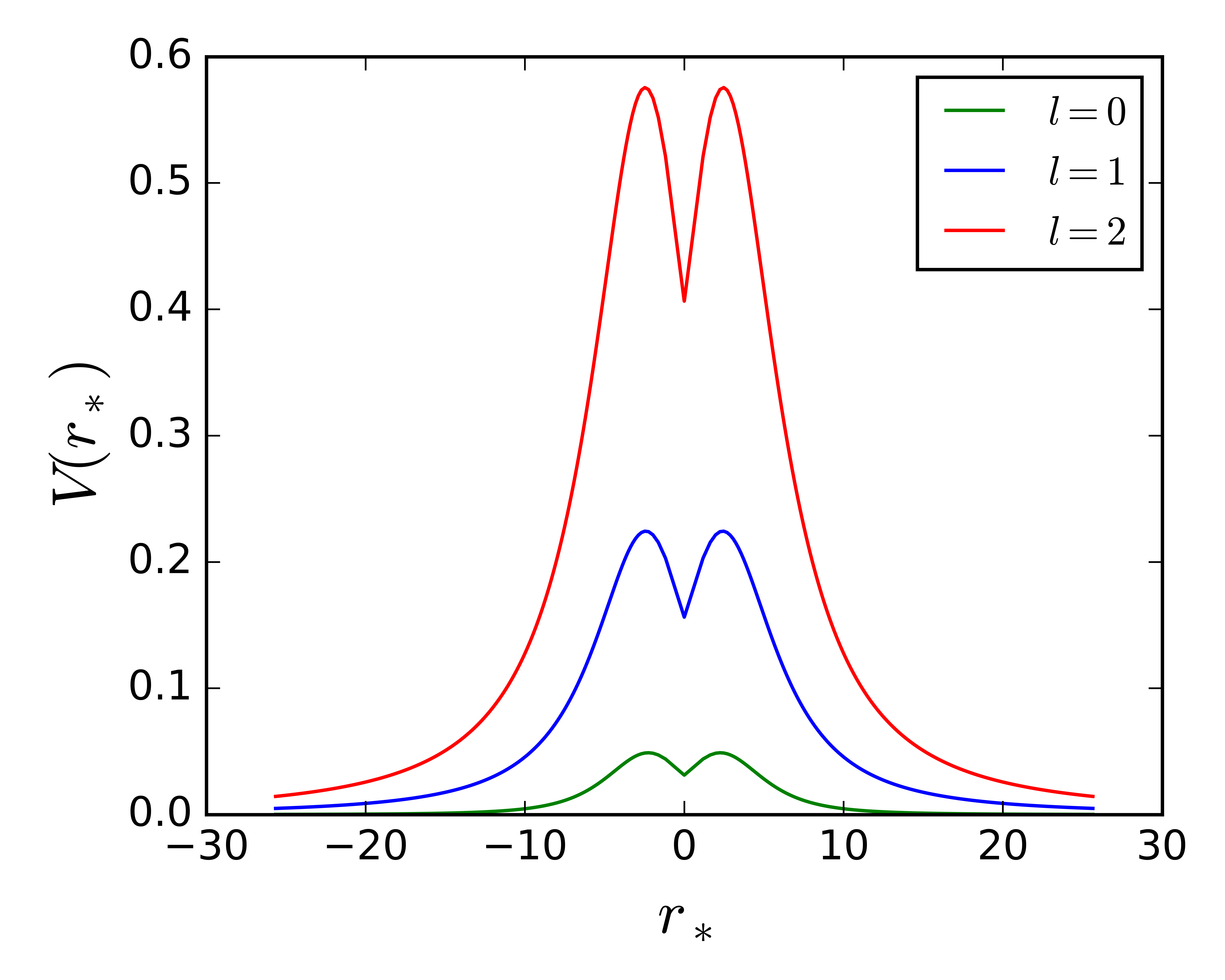
(a) $\kappa=\lambda=0.5,M=1$

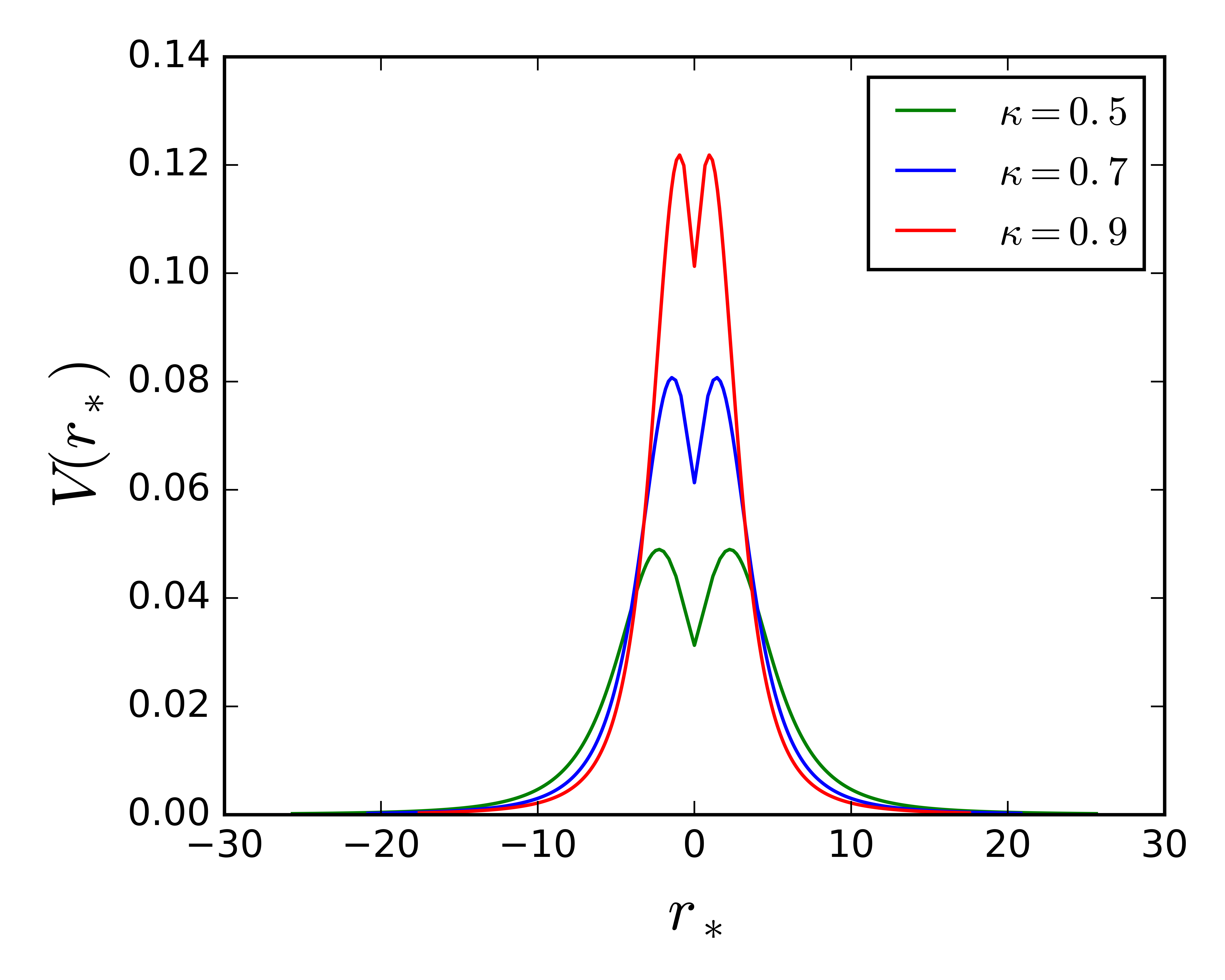
(b) $l=0,\lambda=0.5,M=1$

Figure 1: Variation of effective potential with the parameters $\kappa$, $\lambda$ and $l$. (a) $\kappa=\lambda=0.5,M=1$, (b) $l=0$, $\lambda=0.5$, $M=1$.

II.3 The breathing mode

In the neighborhood of the detector, the background spacetime is flat and we consider the perturbation of a flat Minkowski background and the constant background scalar field,

$$g_{\mu\nu}=\eta_{\mu\nu}+h_{\mu\nu},\;\;\;\;\Phi=\Phi_{0}(1+\epsilon)$$ (13)

where $\Phi_{0}$ is a constant. The field equations become

$$\Box(-h_{\mu\nu}+\eta_{\mu\nu}\epsilon)=\frac{2{\bar{\kappa}}}{l\Phi_{0}}T_{\mu\nu}$$ (14)

$$\Box\epsilon=\frac{\bar{\kappa}}{l{\Phi}_{1}}T$$ (15)

where ${\Phi}_{1}=\frac{3\Phi_{0}}{1+\Phi_{0}}$. Here the choice of gauge is

$$\partial_{\nu}\bar{h}^{\mu\nu}=\partial^{\mu}\epsilon$$ (16)

where ${\bar{h}}^{\mu\nu}$ is the trace-reversed metric perturbation. In vacuum, we have $\Box h_{\mu\nu}=0=\Box\epsilon$ and in the transverse traceless gauge, we get

$$h_{\mu\nu}=\begin{bmatrix}0&0&0&0\\ 0&h_{+}-\epsilon_{0}&h_{\times}&0\\ 0&h_{\times}&-h_{+}-\epsilon_{0}&0\\ 0&0&0&0\end{bmatrix}e^{i\omega(t-z)}$$ (17)

for a plane wave propagating in the $z$-direction. The scalar field is $\Phi=\Phi_{0}(1+\epsilon)$ where

$$\epsilon=\epsilon_{0}e^{i\omega(t-z)}$$ (18)

Due to the presence of the scalar field, there is an additional polarization in the gravitational wave, which is known as the breathing mode breathing . Usually, if we consider a massive scalar, then we also have a longitudinal mode. However, in our work here, we consider only a massless scalar.

In a curved background, the equation for scalar field perturbation is,

$$\Box(\delta\Phi)=g^{\mu\nu}\delta\Gamma^{\alpha}_{\mu\nu}\partial_{\alpha}\Phi+h^{\mu\nu}A_{\mu\nu}-B\,\delta\Phi-C^{\alpha}\partial_{\alpha}(\delta\Phi)$$ (19)

where we have defined,

$$A_{\mu\nu} = \frac{\Omega^{\prime}}{2\Omega+3}\Phi_{;\mu}\Phi_{;\nu}+\Phi_{;\mu;\nu}$$ (20)

$$B = \frac{2\bar{\kappa}}{l}\frac{\Omega^{\prime}T^{b}}{(2\Omega+3)^{2}}+\frac{\Phi^{;\alpha}\Phi_{;\alpha}}{2\Omega+3}\left(\Omega^{\prime\prime}-\frac{2(\Omega^{\prime})^{2}}{2\Omega+3}\right)$$ (21)

$$C^{\alpha} = \frac{2\Omega^{\prime}}{2\Omega+3}\Phi^{;\alpha}$$ (22)

Here a prime denotes a derivative w.r.t $\Phi$ and we have assumed that there is no fluctuation of $T^{b}$, the trace of matter stress energy (i.e. $\delta T^{b}=0$). A similar equation in the Einstein frame is obtained in zimmerman . If we can make an infinitesimal gauge transformation ($h_{\mu\nu}\rightarrow h_{\mu\nu}+\xi_{\mu;\nu}+\xi_{\nu;\mu}\,,\delta\Phi\rightarrow\delta\Phi+\xi^{\mu}\partial_{\mu}\Phi$ generated by $x^{\mu}\rightarrow x^{\mu}-\xi^{\mu}$) which satisfies,

$$\left\{\Box\xi^{\alpha}-\xi^{\mu}R^{\alpha}_{\;\;\mu}-B\,\xi^{\alpha}\right\}\Phi_{;\alpha}+\xi^{\mu;\nu}\left(2A_{\mu\nu}-\Phi_{;\mu}C_{\nu}\right)-C^{\alpha}\Phi_{;\mu;\alpha}\xi^{\mu}=C^{\alpha}\partial_{\alpha}\delta\Phi-h^{\mu\nu}A_{\mu\nu}+B\,\delta\Phi-(h^{\alpha\nu}_{\,\,\,\,;\nu}-\frac{1}{2}h^{;\alpha})\Phi_{;\alpha}$$ (23)

where $\xi^{\alpha}$ is the gauge function, the equation for scalar field perturbations reduces to,

$$\Box(\delta\Phi)=0$$ (24)

It can be easily shown that (23) always admits a solution. For example, since the background spacetime and the scalar field are static and spherically symmetric, we may choose the gauge function to be $\xi^{\mu}=(\xi^{t},0,0,0)$. With this choice, it turns out that all second derivative terms in the equation for $\xi^{\mu}$ vanish and (23) reduces to the form $\frac{\partial\xi^{t}}{\partial t}=f(h_{\mu\nu};\delta\Phi;x^{\mu})$, which can always be integrated.

Since the scalar perturbation obeys the Klein-Gordon equation in the fixed background metric, the QNMs calculated may correspond to the breathing mode mentioned earlier. The metric and the scalar field fluctuations produce the gravitational wave that is detected by detectors situated in the asymptotic region where the background spacetime can be approximated as flat. The scalar field fluctuation produces a breathing mode polarization in the GWs. The strain excitation in a single detector is a combination of the projections of the gravitational waveforms corresponding to the different polarization states incident on it isi . In general it is not possible to isolate with quadrupolar detectors even the two polarization components predicted in General Relativity from observations of a single detector Pai:2000zt , let alone the five polarization states, which is the maximum number of non-degenerate states that metric theories of gravity are allowed will . With at least five linearly independent detectors it is possible to resolve these five polarizations from transient signals will ; dhurandhartinto . However, that solution is beyond the scope of this work; rather, here we shall consider only the breathing mode, and use the QNMs calculated to find the errors on the estimated metric parameters using a Fisher matrix analysis.

We now proceed towards obtaining the time-domain profiles and the QNMs, which will provide inputs for parameter estimation using GW data.

III Time-domain profile and quasinormal modes

To begin, let us first look at the time-domain profile of the scalar field and then find the quasi-normal modes.

III.1 Time domain profile

The time evolution of the scalar field is obtained by directly integrating the differential equation following the method described in qnmreview1 , gundlach . We can write the scalar field equation without imposing the stationary ansatz as,

$$\frac{\partial^{2}\psi_{lm}}{\partial t^{2}}-\frac{\partial^{2}\psi_{lm}}{\partial r_{*}^{2}}+V_{l}(r_{*})\psi_{lm}=0$$ (25)

Rewriting the wave equation in terms of light cone coordinates, $du=dt-dr_{*}$ and $dv=dt+dr_{*}$ we obtain,

$$\left(4\frac{\partial^{2}}{\partial u\partial v}+V_{l}(u,v)\right)\psi_{lm}=0$$ (26)

In these coordinates, the time evolution operator is,

$$\exp\left(h\frac{\partial}{\partial t}\right) =\exp\left(h\frac{\partial}{\partial u}+h\frac{\partial}{\partial v}\right)$$ (27)

$$=-1+ \exp\left(h\frac{\partial}{\partial u}\right)+\exp\left(h\frac{\partial}{\partial v}\right)+\frac{h^{2}}{2}\left(\exp\left(h\frac{\partial}{\partial u}\right)+\exp\left(h\frac{\partial}{\partial v}\right)\right)\frac{\partial^{2}}{\partial u\partial v}+O(h^{4})$$

By acting this operator on $\psi_{lm}$ and using (26), we arrive at

$$\psi_{lm}(u+h,v+h)= \psi_{lm}(u+h,v)+\psi_{lm}(u,v+h)-\psi_{lm}(u,v)$$

$$-\frac{h^{2}}{8}V_{l}(u,v)\left(\psi_{lm}(u+h,v)+\psi_{lm}(u,v+h)\right)+O(h^{4})$$ (28)

Using the above equation, we can calculate the values of $\psi_{lm}$ inside the square which is built on the two null surfaces $u=u_{0}$ and $v=v_{0}$, starting from the initial data specified on them. The plots (Figure 2) below show the time domain profile of the field calculated for various parameter values. For the $v=0$ null line, a Gaussian profile of width $14$ centered at $u=10$ is assumed. On the $u=0$ line we have assumed constant data. The field has been calculated in the region $0<u<200$ and $0<v<200$ with a step-size of $h=0.1$. Figure 2 shows the time domain profiles for various values of the parameters.

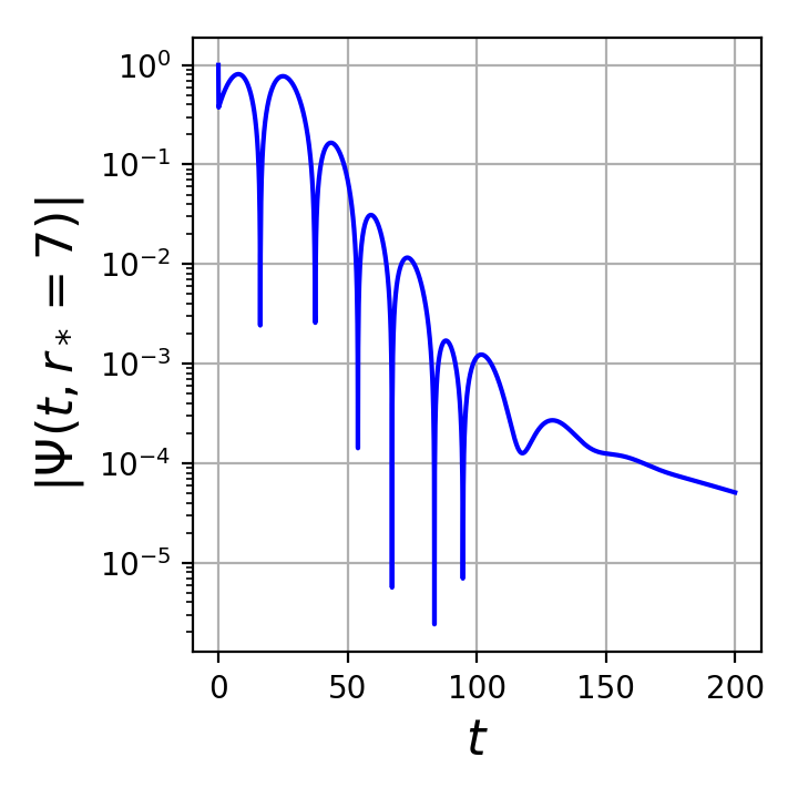
(a) $l=0$

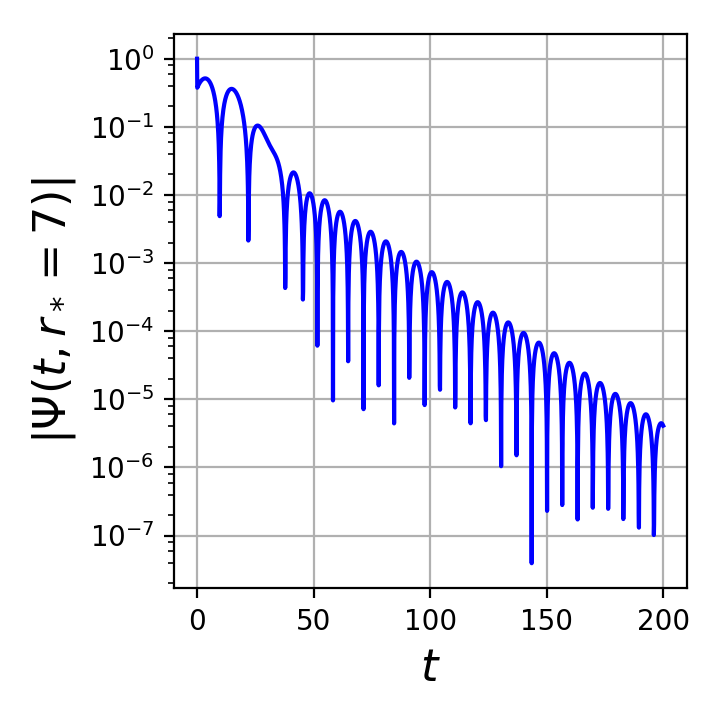
(b) $l=1$

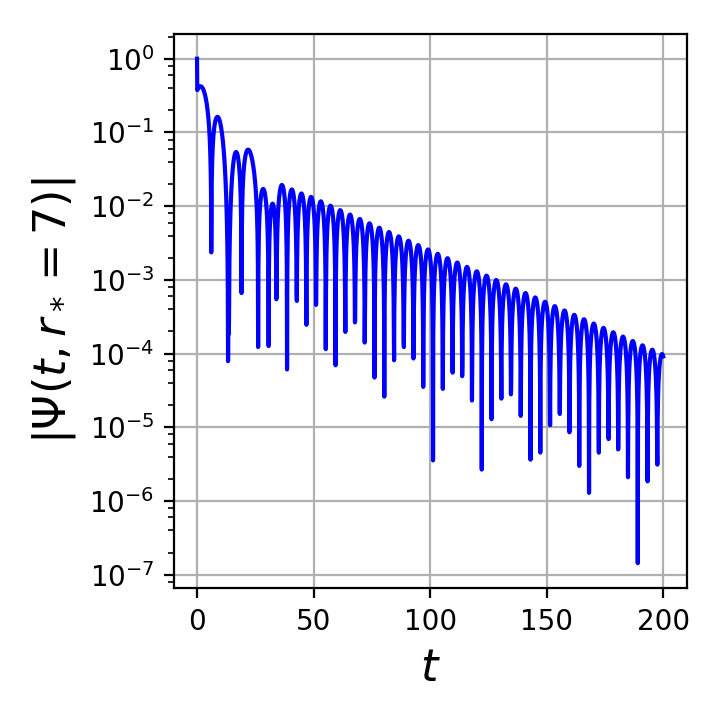
(c) $l=2$

Figure 2: Time domain profile and quasinormal ringdown. Profiles have been calculated for $\kappa=0.5=\lambda$, $M=1$ and $l=0,1,2$ at $r_{*}=7$. Initial conditions are $\psi_{lm}(u,0)=\exp\left[-\frac{(u-10)^{2}}{100}\right]$ and $\psi_{lm}(0,v)=1$. The integration grid is $u,v\in(0,200)$ with $h=0.1$. (a) l=0, (b) $l=1$ and (c) $l=2$.

III.2 Quasi-normal modes

The quasinormal modes, first discussed in vishu , are defined as complex eigenfrequencies of the wave equation (11) which satisfies the boundary conditions $\psi_{lm}\sim e^{\pm i\omega r_{*}}$ in the asymptotic regions $r_{*}\rightarrow\pm\infty$ qnmreview1 ; qnmreview2 . At the throat, we impose the continuity of $d\psi_{lm}/dr_{*}$. Since the potential is symmetric about $r_{*}=0$, the eigenfunctions should be either symmetric or antisymmetric. Thus, we get two families of QNMs corresponding to the initial conditions $\psi_{lm}(0)=0$ and $\psi_{lm}^{\prime}(0)=0$, that can be obtained by a direct integration of the wave equation paniqnm .

In the asymptotic region we solve (11) by expanding $\psi_{lm}$ as a power series upto a finite but arbitrary order,

$$\psi_{lm}=e^{kr_{*}}\sum_{n=0}^{N}\frac{a_{n}}{r^{n}}=e^{kr}r^{kM(1+\lambda)}\sum_{n=0}^{N}\frac{\bar{a}_{n}}{r^{n}}$$ (29)

where we have used the asymptotic expansion of $r_{*}(r)$ in (29). By substituting (29) into (11) and expanding it in terms of $1/r$ we can solve for the coefficients $\bar{a}_{1},\bar{a}_{2},\bar{a}_{3},...$ in terms of $\bar{a}_{0}$. Near $2M$ we expand $\psi_{lm}$ as,

$$\psi_{lm}=\sum_{n=0}^{N^{\prime}}b_{n/2}(r-2M)^{n/2}$$ (30)

Using the same method as stated above, $b_{1},b_{3/2},b_{2}...$ can be solved in terms of $b_{0}$ and $b_{1/2}$. The tortoise coordinate, given in (10), near $r=2M$ can be written as,

$$r_{*}=c_{1/2}(r-2M)^{1/2}+c_{1}(r-2M)+c_{3/2}(r-2M)^{3/2}+....$$ (31)

From (30) and (31) we get,

$$\left.\frac{d\psi_{lm}}{dr_{*}}\right|_{r_{*}=0}=\frac{b_{1/2}}{c_{1/2}}$$ (32)

Thus, we calculate the QNMs by integrating the wave equation from $r_{0}=2M(1+\delta)$ (where $\delta\||1$) to a large value of $r$ and comparing it with the two independent solutions obtained by substituting $k=\pm i\omega$ in (29). This gives two families of QNMs by starting with either $b_{0}=0$ or $b_{1/2}=0$, which corresponds to the initial conditions $\psi_{lm}(0)=0$ and $\psi_{lm}^{\prime}(0)=0$ respectively.

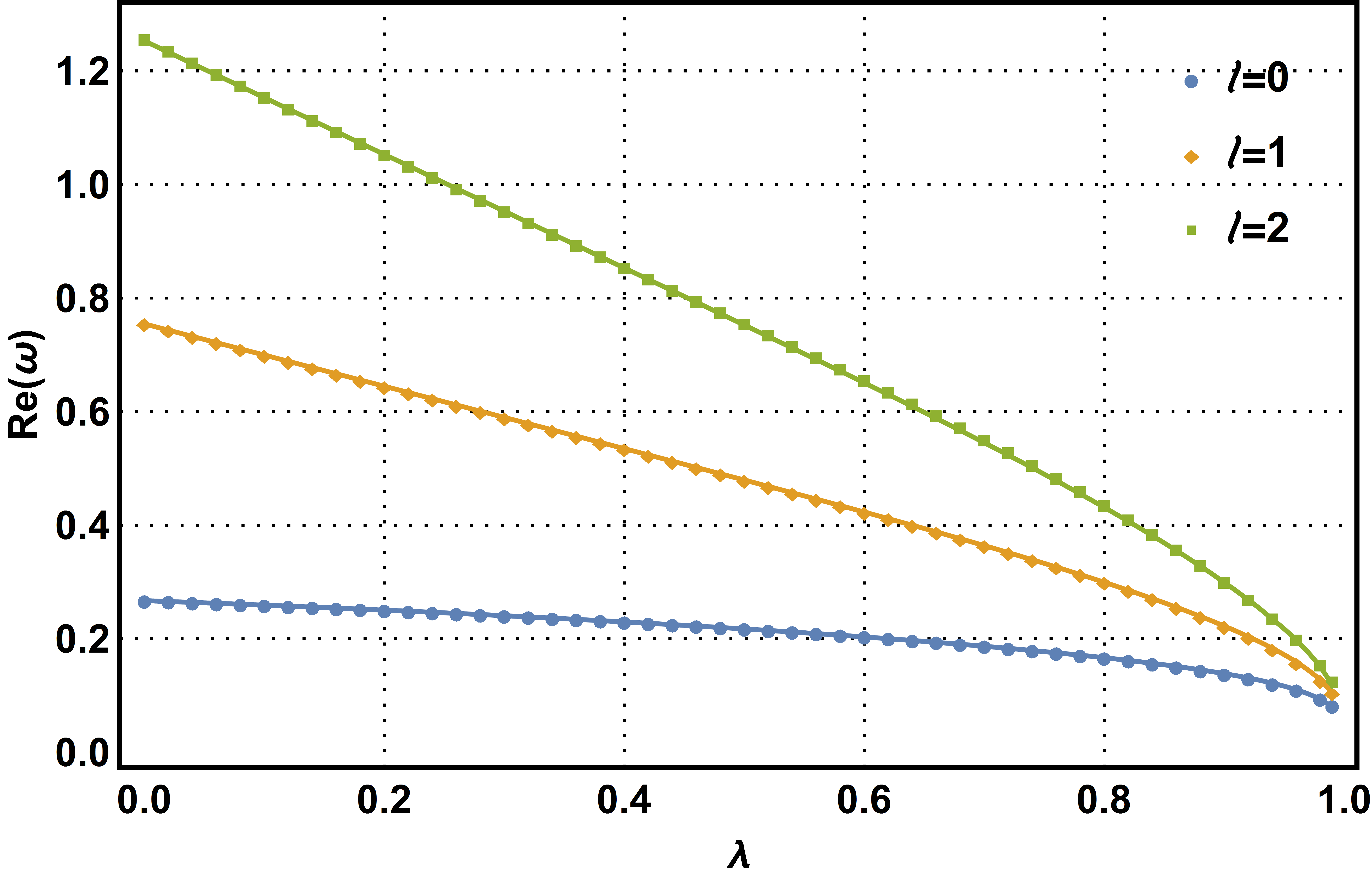
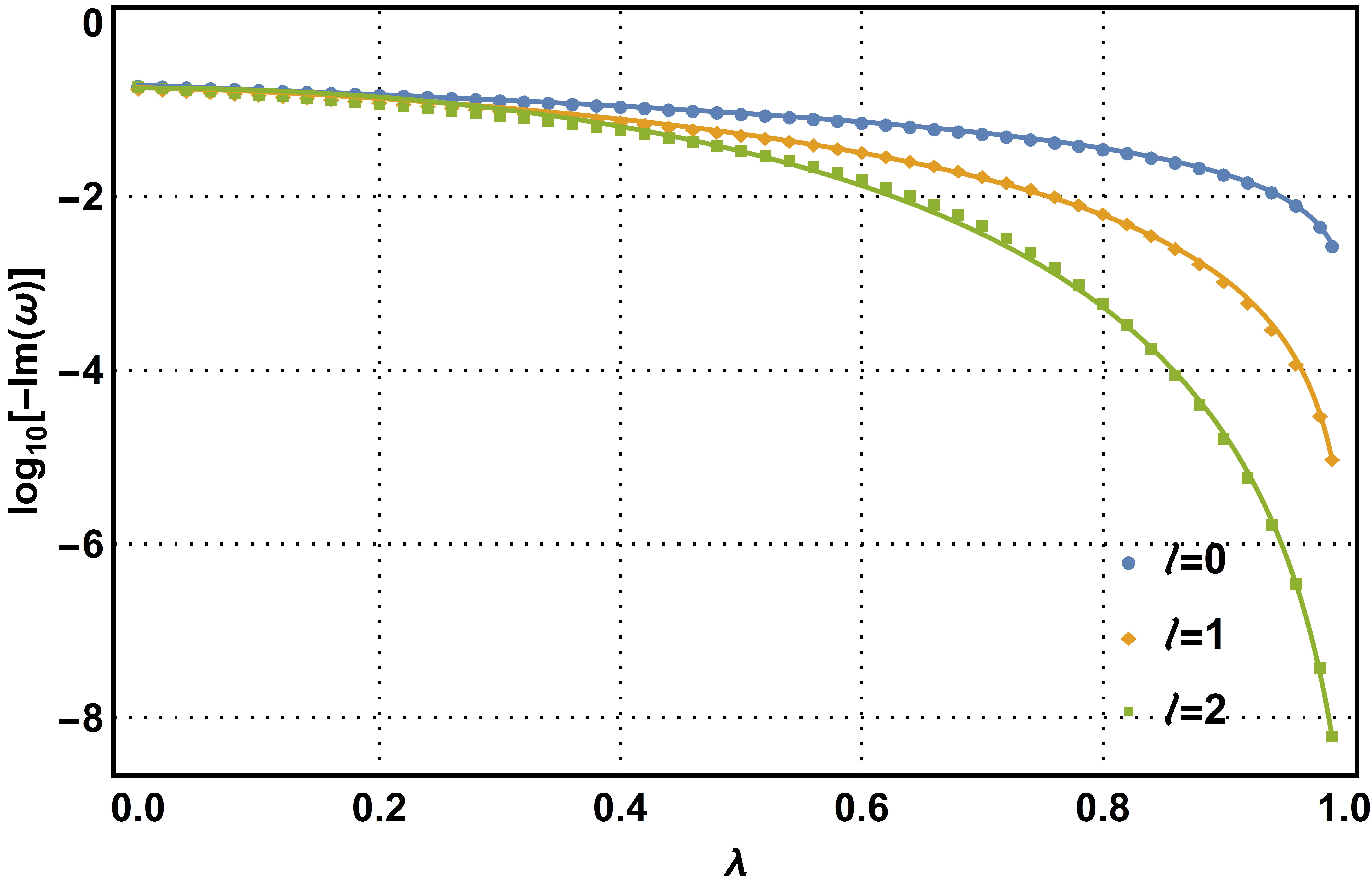
Figure 3: Real and imaginary parts of QNFs are plotted w.r.t $\lambda$. Here $M=1$ and $\kappa=1-\lambda$. Frequencies for all other values of $\kappa$, $\lambda$ and $M$ can be obtained from this data. The smooth curve joining the data points is the analytical fit which is obtained in the next section.

The values of $\omega$ vs $\lambda$ for $l=0,1,2$ are shown in the Figure (3). Here, as before, $\kappa+\lambda=1$ and $M=1$ is assumed. $\lambda=0$ is an ultrastatic spacetime and $\lambda=1$ is the Schwarzschild limit. $\omega$ is given in geometric units. Quasinormal frequencies can also be calculated directly from the time domain profile (Figure 2) by fitting it with damped sinusoids using Prony fit method qnmreview1 (see Fig. 4). Few of the frequencies obtained through both direct integration and Prony fit methods are given in Table 1. Both the methods are found to be consistent with each other.

$\kappa$	$\lambda$	$l$	$\omega_{prony}$	$\omega_{DI}$
0.9	0.1	2	$1.15101310-0.14169729i$	$1.15097690-0.14490430i$
0.7	0.3	2	$0.94816165-0.08240778i$	$0.94989921-0.08342129i$
0.5	0.5	2	$0.75002394-0.03201102i$	$0.75225700-0.03285035i$
0.4	0.6	2	$0.65230556-0.01514451i$	$0.65232260-0.01512223i$
0.2	0.8	2	$0.43641027-0.00040061i$	$0.43221577-0.00056867i$

Table 1: QNMs computed through Prony fit of time domain profile and direct integration

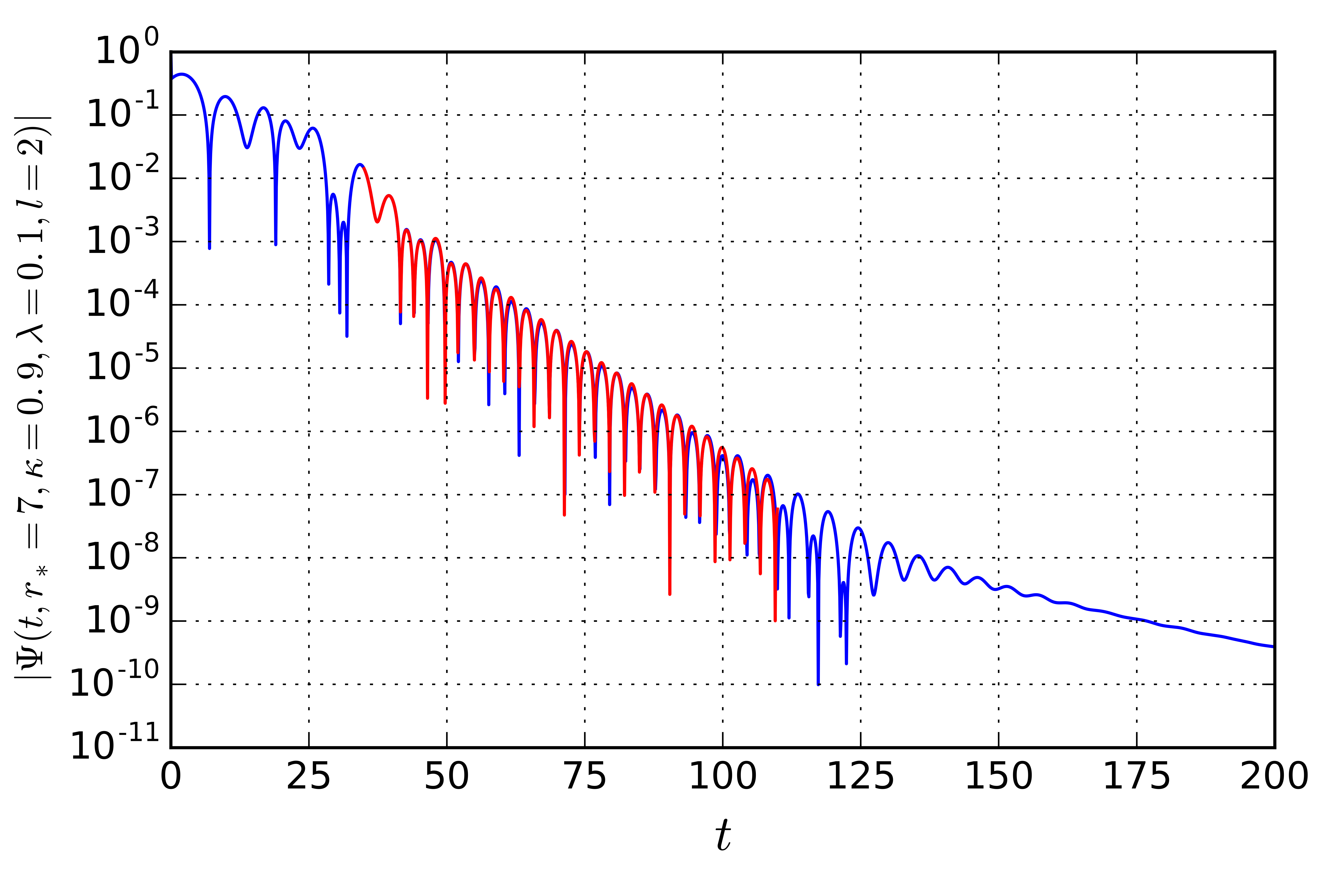
Figure 4: An example of Prony fit of time domain profile. The data is fitted with four complex frequencies.

III.3 Approximate Analytic Fit

In order to perform parameter estimation on the gravitational waves comprised of QNMs, we need to calculate the derivatives of QNMs with respect to $\frac{\kappa}{\lambda}$ and $M$. For this, we construct an approximate model for $\omega$ as follows (here $\kappa=1-\lambda,M=1$),

$$\begin{split}\omega_{re}=(a-b\lambda)(1-\lambda^{n})^{m}\\ \ln(-\omega_{im})=c+d\ln\left(1-p\lambda^{q}\right)\\ \omega=\omega_{re}+i\omega_{im}\end{split}$$ (33)

The values of $a,b,c,d,m,n,p,q$ were calculated using NonlinearModelFit in Mathematica Mathematica . For $l=0$,

$$\begin{split}\omega_{re}&=(0.27-0.08\lambda)(1-\lambda^{2.36})^{0.24}\\ \omega_{im}&=-0.19(1-0.99\lambda^{0.94})^{1.02}\end{split}$$ (34)

For $l=1$,

$$\begin{split}\omega_{re}&=(0.75-0.55\lambda)(1-\lambda^{7.95})^{0.28}\\ \omega_{im}&=-0.18(1-0.99\lambda^{1.41})^{2.63}\end{split}$$ (35)

and for $l=2$, we have

$$\begin{split}\omega_{re}&=(1.25-\lambda)(1-\lambda^{8.87})^{0.33}\\ \omega_{im}&=-0.18(1-0.96\lambda^{1.99})^{6.05}\end{split}$$ (36)

Figure 3 shows the plots of analytical model of the QNMs. Since at infinity $d\tau=(\kappa+\lambda)dt$, the frequency of the signal measured by an observer at the asymptotic region will be $\nu=\frac{\omega_{re}}{2\pi(\kappa+\lambda)}$ and the time constant will be $\tau=\frac{\kappa+\lambda}{|\omega_{im}|}$. Thus, for $l=0$,

$$\begin{split}\nu=&\frac{8628.13}{M}\left(1-0.29\frac{\lambda}{\lambda+\kappa}\right)\left(1-\left(\frac{\lambda}{\lambda+\kappa}\right)^{2.36}\right)^{0.24}Hz\\ \tau=&\frac{M}{38908.58}\left(1-0.99\left(\frac{\lambda}{\lambda+\kappa}\right)^{0.94}\right)^{-1.02}s\end{split}$$ (37)

For $l=1$,

$$\begin{split}\nu=&\frac{24375.84}{M}\left(1-0.73\frac{\lambda}{\lambda+\kappa}\right)\left(1-\left(\frac{\lambda}{\lambda+\kappa}\right)^{7.95}\right)^{0.28}Hz\\ \tau=&\frac{M}{36290.32}\left(1-0.99\left(\frac{\lambda}{\lambda+\kappa}\right)^{1.41}\right)^{-2.63}s\end{split}$$ (38)

For $l=2$,

$$\begin{split}\nu=&\frac{40478.89}{M}\left(1-0.80\frac{\lambda}{\lambda+\kappa}\right)\left(1-\left(\frac{\lambda}{\lambda+\kappa}\right)^{8.87}\right)^{0.33}Hz\\ \tau=&\frac{M}{36026.46}\left(1-0.96\left(\frac{\lambda}{\lambda+\kappa}\right)^{1.99}\right)^{-6.05}s\end{split}$$ (39)

$M$ is in units of solar mass, $\nu$ is in Hz and $\tau$ is in seconds. Moreover, the validity of the above fits is verified for $\frac{\kappa}{\lambda}$ larger than a few times 0.001.

The gravitational-wave strain in a detector is a linear function of the various polarization components the theory may allow,

$$h(t)=\sum_{A}F^{A}h_{A}\,,$$ (40)

where $A$ is the polarization index, $h_{A}$ are GW polarization components, and the coefficients $F^{A}$ are the antenna-pattern functions that are determined by how well the polarization components project on the GW detector. The $F^{A}$ depend on the sky-position angles $(\vartheta,\varphi)$ of the source and the polarization angle of the gravitational wave, in general. In our case, the source is the wormhole studied here. The contribution to the detector strain from the breathing mode alone of such a source will be considered in this work, and is given by

$$h(t)=A\sin(2\pi\nu t)e^{-t/\tau}\,,$$ (41)

where the strain amplitude $A$ contains the breathing-mode antenna pattern isi

$$F^{b}=-\frac{1}{2}\sin^{2}\vartheta\cos 2\varphi\,.$$ (42)

Above, $\vartheta$ and $\varphi$ are the polar angle and azimuthal angle, respectively, that define the sky-position of the source in a coordinate system where the two arms of the quadrupolar detector are the $x$ and $y$ axes. Therefore, the strength of the detector signal, which depends on $h$ linearly, will vary across the sky even if the rest of the wormhole parameters remain unchanged. Below, for estimating parameter errors, we will take the source to be located along the $x$ or $y$ arm of the detector, i.e., $\vartheta=\frac{\pi}{2}$ and $\varphi=0$ or $\pi/2$.

If a loud enough damped-sinusoid strain signal (41) is observed in a detector, the parameters of the wormhole can be deduced from a straightforward Fourier transform. For example, by an observation of the $l=0$ signal in Eq. (37), one can infer from its measured central frequency $\nu$ and the time-constant $\tau$, the mass $M$ and geometry parameter $\kappa/\lambda$. When the signal is strong enough to allow the observation of multiple modes – the higher modes will get progressively weaker inherently, but their signal-to-noise ratio will also depend on the amplitude of the detector noise at the mode frequency – the multiple measured mode frequencies and time-constants can be used to perform self-consistency checks or even rule out a wormhole as the source of the signals.

Note that other sources of damped-sinusoid signals can exist in the GW detectors, both astrophysical and terrestrial in origin BDGL ; Bose:2016sqv . To improve the odds of the former, it is important to observe the commensurate signals in multiple GW detectors Bose:1999pj ; Pai:2000zt . But to distinguish one astrophysical source from another, e.g., QNMs of black holes in General Relativity Talukder:2013ioa or other braneworld models Seahra:2004fg ; Chakraborty:2017qve , further comparative studies of their signals are required.

A remaining practical issue is that signals will typically be immersed in detector noise, and the measurement of any of their parameters will have errors. This is what we study next.

IV Gravitational wave observations of the modes

We use the Fisher information-matrix formalism Helstrom to estimate how accurately the wormhole parameters will be measurable using interferometric detectors like aLIGO. To estimate the error in $\kappa/\lambda$, we compute that matrix for the damped-sinusoid signal (41) in a single aLIGO detector at design sensitivity aLIGOZDHP for that parameter alone. The matrix is determined by the derivative of the signal $h$ with respect to $\kappa/\lambda$, which influences both the frequency and the damping time-constant of the signal. For this first study, we take $M$ to be known. For wormholes that result from the merger of two black holes this parameter can be estimated from the inspiral part of the signal. Even so, such an estimation also requires knowledge of the strength of the signal. Currently, it is not understood how large the QNM amplitude of these wormholes can be, whether they form in binary black hole merger processes or otherwise. Therefore, for reference we take the maximum QNM strain amplitude to be $10^{-21}$, which is approximately the maximum amplitude of the GW150914 signal gwobs1 . We recognize that this choice is arbitrary. If at a later date realistic amplitudes are deduced theoretically or numerically, then the errors obtained in this paper should be scaled appropriately by using those values. Finally, we invert the information matrix to derive the estimated variance in the measured values of $\kappa/\lambda$ Helstrom . Its square-root gives the lower bound on the statistical error in $\kappa/\lambda$. To deduce the error for multiple statistically independent observations, one simply replaces the information matrix for a single observation in the above procedure with the sum of the information matrices for multiple observations.

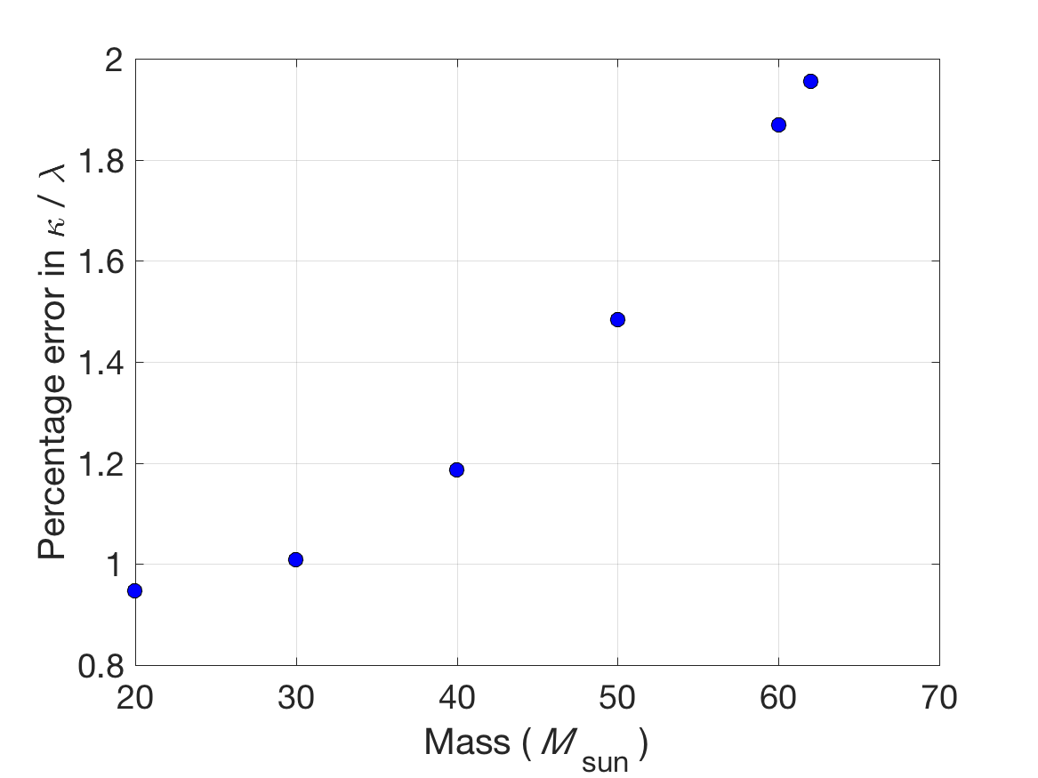
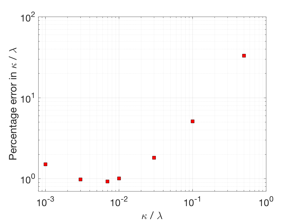
Figure 5: The estimated statistical error in $\kappa/\lambda$ (in percentage) is shown for various values of the wormhole mass $M$ (in the left figure, where $\kappa/\lambda$ is kept fixed at 0.01) and the wormhole parameter $\kappa/\lambda$ (in the right figure, where $M$ is kept fixed at $30M_{\odot}$). These estimates were obtained for gravitational-wave observations of the breathing mode of the wormhole solution studied here with a detector like aLIGO. The maximum amplitude of the mode in all cases is set to be $10^{-21}$, which is approximately the peak amplitude of GW150914, whose final detector-frame mass had a median value of about $68M_{\odot}$. The wormhole QNM frequency for $l=0$ is 64 Hz for $M=68M_{\odot}$ and $\kappa/\lambda=0.1$. For comparison, the frequency of the $l=2$, $m=2$ QNM of GW150914 was at or above $\simeq 243$ Hz gwobs1 . The error in $\kappa/\lambda$ increases with $M$ (left figure) primarily because the mode frequency decreases, thereby, placing the signal in less sensitive part of the detector band. The right figure shows that the error in $\kappa/\lambda$ initially reduces when the value of that parameter is increased. This happens because the mode frequency shifts to more sensitive parts of the detector band (from 64 Hz at $\kappa/\lambda=3\times 10^{-3}$ to 85 Hz at $\kappa/\lambda=10^{-2}$). For higher values of $\kappa/\lambda$, the error increases owing to decreasing time constant (and, therefore, the effective integration duration) of the mode.

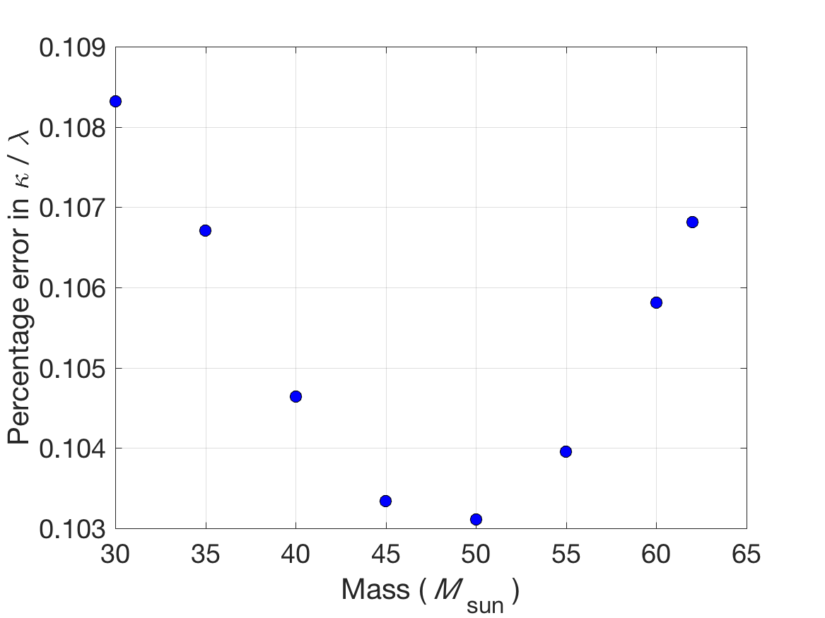
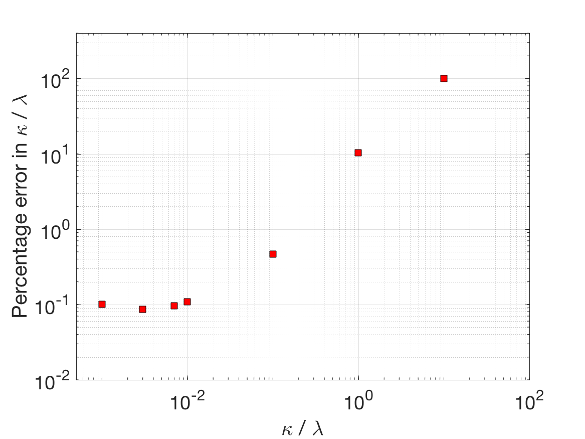
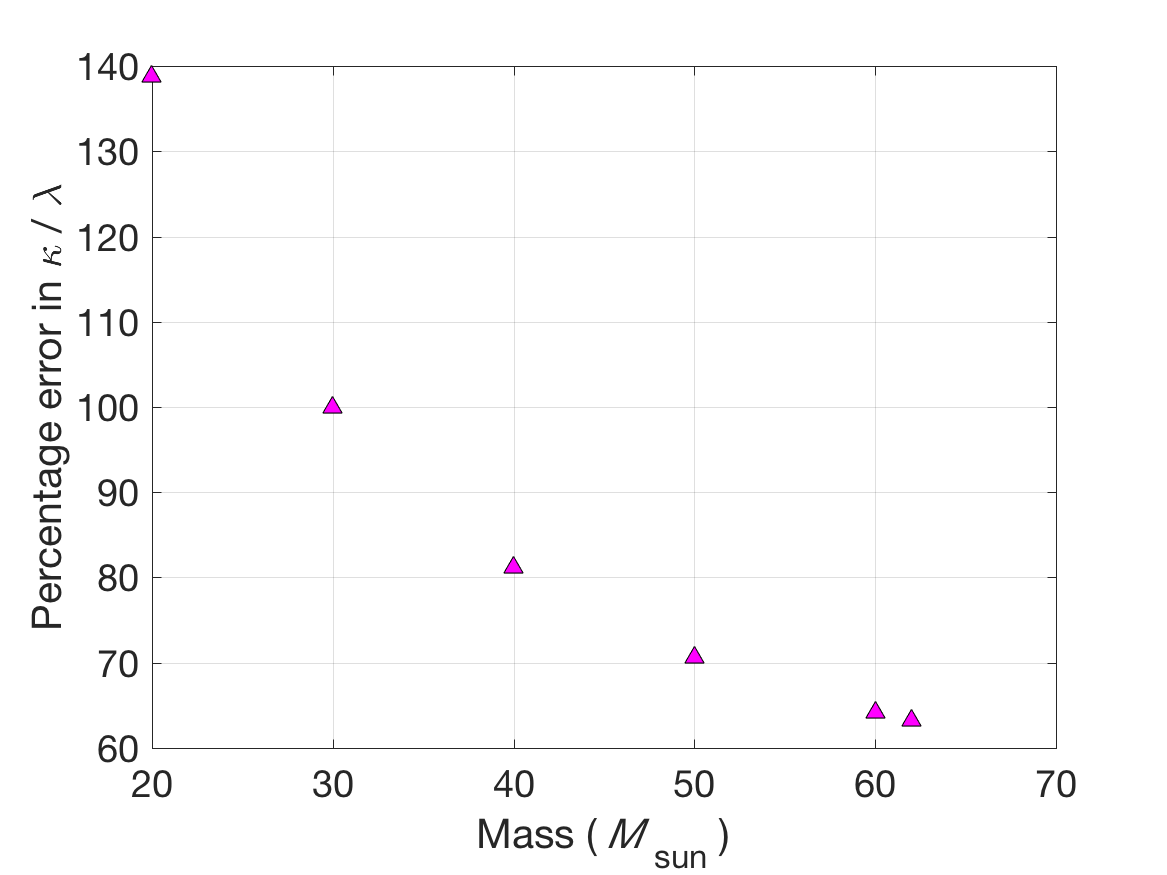
Figure 6: The two left-most plots are similar to the ones shown in Fig. 5, but for the Einstein Telescope Hild . The right-most plot is for $\kappa/\lambda=10$ and the Einstein Telescope; it is interesting how the error decreases with increasing mass for the mass range shown here, before it rises again (not shown) owing to the signal frequency moving into the low-frequency seismic band). Moreover, whereas $\kappa/\lambda<1$ in Fig. 5 here we raise that limit in the middle and right plots.

The parameter errors in $\kappa/\lambda$ are plotted in Figs. 5 and  6 for observations of the breathing mode of the wormhole described above in an aLIGO and Einstein Telescope detector, respectively. This is an optimistic estimate since errors in other source parameters, such as the signal’s time of arrival and $M$, and their covariances, which were neglected here, can worsen the estimation of $\kappa/\lambda$. Moreover, while the SNR of the complete signal of GW150914 was moderately high, that of the post-merger signal was not. Hence, the Fisher estimates, which we base on the peak amplitude of the merger signal, must be followed up with more reliable parameter estimation analyses; this preliminary study therefore makes the case for adapting a more realistic approach in a future work for estimation of $\kappa/\lambda$. Such an approach can be the use of Monte Carlo methods, as demonstrated for binary black hole parameter estimation in Ref. Ajith:2009fz , or Bayesian methods, such as that used in Ref. DelPozzo:2013ala for combining the posteriors of the tidal deformability parameter, which describes neutron star composition, from multiple binary neutron star coalescences. Indeed, an exercise that can be performed is the improvement in the estimation for $\kappa/\lambda$ by combining multiple observations. One way to do that would be to compute a joint posterior. Another, less optimal method, would be to stack-up the power from the multiple signals, as was done for estimating the post-merger oscillation parameters of hypermassive neutron stars in Ref. Bose:2017jvk . Since Figs. 5 and  6 suggest a wide enough range of $\kappa/\lambda$ where its value may be measurable fairly accurately, e.g., to distinguish the wormhole geometry from Schwarzschild, it appears to be worthwhile to pursue these more sophisticated, and computationally expensive methods, in the future.

V Conclusions

In summary, we obtained the following results in this work.

Assuming a two-parameter family of wormholes that arise in a scalar-tensor theory of gravity, we have first derived their scalar quasinormal modes using standard numerical methods. We have cross-checked our numerical methods with known results on QNMs in other wormhole geometries available in the literature taylor . The QNMs obtained and their variation w.r.t. the parameters were then fitted using methods of non-linear least square fitting. These results were then used to estimate the accuracy with which the wormhole parameter $\kappa/\lambda$, which appears in the line element, can be measured using inputs from GW observations. For this first study, we kept things simple by considering the measurement of just one parameter (i.e., $\frac{\kappa}{\lambda}$), while treating $M$, which is related to the throat radius, as known precisely. While it is true that energy conservation will require $M$ to be bounded from above by the total mass of the binary black hole merger that produces it, and that this mass is measurable from observations of the inspiral phase, it is not clear yet how it determines $M$. This matter is left for future exploration.

Under the aforementioned assumptions, we find that for a certain range of the wormhole parameter it would be possible to estimate its value from adequately loud signals, if not in aLIGO, then in the Einstein Telescope (ET). For example, if the maximum amplitude of the breathing mode is set to be $10^{-21}$, which is approximately the peak amplitude of GW150914, the error in that parameter can be measured to within tens of percent for $\log_{10}(\kappa/\lambda)\in(-3,-1)$ in an aLIGO-like detector at design sensitivity. This can be seen in the right figure in Fig. 5. There we set the $M=30M_{\odot}$, which describes a wormhole that may form from the merger of stellar mass black holes that are not too heavy. For larger $M$, the error in $\kappa/\lambda$ will be larger. Moreover, for possible wormholes resulting from the merger of black holes of the type observed by LIGO and Virgo so far, one can determine $\kappa/\lambda$ in ET to within a few to several tens of percent as well for $\kappa/\lambda\leq 10$ (see Fig. 6) and, therefore, distinguish them from Schwarzschild (albeit, for non-spinning geometries). The important caveat is that these error estimates are expected to worsen when one expands the parameter space by including spin and accounts for the error in the wormhole mass and any covariances that may arise among those two parameters and $\kappa/\lambda$.

Significantly, since mergers can leave behind remnants with non-vanishing angular momentum, it is important to extend the results here by introducing rotation in the wormhole line element, thereby making it more realistic. Rotating wormholes have been studied in the literature teo . QNMs for rotating Ellis wormholes have been discussed in ringdown3 . For the line element used in this article, one would first have to generalize it by including rotation. More importantly, one would first need to do this in the scalar-tensor theory and, subsequently, study the consequences for the WEC, if any. This may be followed up by finding the QNMs and, thereafter, the estimates of parameter errors in possible GW observations, now using additionally the spin parameter.

The real question however is whether one can obtain a wormhole metric as a result of an astrophysical merger process. There are some simplistic models of mergers which are analytic in nature emparan . These could be viable starting points for understanding whether a wormhole could be created at all in a merger.

References

- (1) A. Einstein and N. Rosen, The Particle Problem in the General Theory of Relativity, Phys. Rev. 48, 73 (1935).
- (2) B. P. Abbott et. al, GW170817: Observation of Gravitational Waves from a Binary Neutron Star Inspiral, Phys. Rev. Letts. 119, 161101 (2017); B. P. Abbott et al., GW151226: Observation of Gravitational Waves from a 22-Solar-Mass Binary Black Hole Coalescence, Phys. Rev. Letts. 116, 241103 (2016); B. P. Abbott et al., GW170104: Observation of a 50-Solar-Mass Binary Black Hole Coalescence at Redshift 0.2, Phys. Rev. Letts. 118, 221101 (2017); B. P. Abbott et al., GW170608: Observation of a 19-solar-mass Binary Black Hole Coalescence, Astrophys. J. 851, no. 2, L35 (2017); B. P. Abbott et al., GW170814: A Three-Detector Observation of Gravitational Waves from a Binary Black Hole Coalescence, Phys. Rev. Letts. 119, 141101 (2017); B. P. Abbott et. al., Binary Black Hole Mergers in the first Advanced LIGO Observing Run, Phys. Rev. X 6, 041015 (2016).
- (3) B. P. Abbott et. al, Observation of Gravitational Waves from a Binary Black Hole Merger, Phys. Rev. Letts. 116, 061102 (2016); B. P. Abbott et al., Tests of General Relativity with GW150914, Phys. Rev. Letts. 116, 221101 (2016).
- (4) A. Einstein, Kosmologische Betrachtungen zur allgemeinen Relativitaetstheorie, Sitzungsberichte der Königlich Preussischen Akademie der Wissenschaften Berlin, part 1, 142 (1917).
- (5) C. W. Misner and J. A. Wheeler, Classical physics as geometry, Ann. Phys. 2, 525(1957).
- (6) H. Ellis, Ether flow through a drainhole: A particle model in general relativity, J. Math. Phys. 14, 104 (1973).
- (7) K. A. Bronnikov, Scalar-Tensor Theory and Scalar Charge, Acta Physica Polonica B4, 251 (1973).
- (8) M. S. Morris, K. S. Thorne and U. Yurtsever, Wormholes, time machines and the weak energy condition, Phys. Rev. Letts. 61, 1446 (1988).
- (9) M. S. Morris and K. S. Thorne, Wormholes in spacetime and their use for interstellar travel: a tool for teaching general relativity, Am. J. Phys. 56, 395 (1988).
- (10) I. D. Novikov, An analysis of the operation of a time machine, Sov. Phys. JETP 68, 439 (1989)
- (11) V. P. Frolov and I. D. Novikov, Physical effects in wormholes and time machines, Phys. Rev. D 42,1057 (1990).
- (12) M. Visser, Lorentzian wormholes: from Einstein to Hawking, AIP Series in Computational and Applied Mathematical Physics, 1996, and references therein.
- (13) A. G. Agnese and M. La Camera, Wormholes in the Brans-Dicke theory of gravitation, Phys. Rev. D 51, 2011 (1995)
- (14) D. F. Torres, G. E. Romero, L. A. Anchordoqui, Might some gamma ray bursts be an observable signature of natural wormholes?, Phys. Rev. D 58, 123001 (1998)
- (15) D. Hochberg and M. Visser, Null Energy Condition in Dynamic Wormholes, Phys. Rev. Letts. 81, 746 (1998)
- (16) C. Barcelo and M. Visser, Traversable wormholes from massless conformally coupled scalar fields, Phys. Letts. B 466, 127 (1999)
- (17) M. Safonova, D. F. Torres and G. E. Romero, Microlensing by natural wormholes: Theory and simulations, Phys. Rev. D 65, 023001 (2001)
- (18) C. Armendariz-Picon, On a class of stable, traversable Lorentzian wormholes in classical general relativity, Phys. Rev. D 65, 104010 (2002)
- (19) J. P. S. Lemos, F. S. N. Lobo and S. Q. de Oliviera, Morris-Thorne wormholes with a cosmological constant, Phys. Rev. D 68, 064004 (2003).
- (20) K. Bronnikov and S. W. Kim, Possible wormholes in a brane world, Phys. Rev. D 67, 064027 (2003)
- (21) S. Sushkov, Wormholes supported by a phantom energy, Phys. Rev. D 71, 043520 (2005)
- (22) F. S. N. Lobo, General class of braneworld wormholes, Phys. Rev. D 75, 064027 (2007)
- (23) N. Tsukamoto, T. Harada and Kajima, Can we distinguish between black holes and wormholes by their Einstein-ring systems?, Phys. Rev. D 86, 104062 (2012).
- (24) S. W. Hawking and G. F. R. Ellis, The large scale structure of spacetime, Cambridge University Press, Cambridge, UK (1973).
- (25) R. M. Wald, General Relativity, University of Chicago Press, USA (1984).
- (26) B. Bhawal and S. Kar, Lorentzian wormholes in Einstein-Gauss-Bonnet theory, Phys. Rev. D 46, 2464 (1992)
- (27) S. Kar, Evolving wormholes and the weak energy condition, Phys. Rev. D49, 862 (1994)
- (28) S. Kar and D. Sahdev, Evolving Lorentzian wormholes, Phys. Rev. D 53, 722 (1996).
- (29) D. Hochberg and M. Visser, The null energy condition in dynamic wormholes, Phys.Rev.Lett. 81, 746 (1998).
- (30) M. Visser, S. Kar and N. Dadhich, Traversable Wormholes with Arbitrarily Small Energy Condition Violations, Phys. Rev. Letts. 90, 201102 (2003).
- (31) S. Kar, N. Dadhich and M. Visser, Quantifying energy condition violations in traversable wormholes, Pramana 63, 859 (2004).
- (32) T. A. Roman, Some thoughts on energy conditions and wormholes, Proceedings of the MG10 Meeting Rio de Janeiro, Brazil, 1909 (2003) and references therein.
- (33) H. Maeda and M. Nozawa, Static and symmetric wormholes respecting energy conditions in Einstein-Gauss-Bonnet gravity, Phys. Rev. D 78, 024005 (2008).
- (34) N. M. Garcia and F. S. N. Lobo, Nonminimal curvature-matter coupled wormholes with matter satisfying the null energy condition, Class.Quant.Grav. 28, 085018 (2011).
- (35) C. G. Boehmer, T. Harko, F. S. N. Lobo, Wormhole geometries in modified teleparallel gravity and the energy conditions, Phys.Rev. D 85, 044033 (2012).
- (36) M. K. Zangeneh, F. S. N. Lobo, N. Riazi, Higher-dimensional evolving wormholes satisfying the null energy condition, Phys. Rev. D 90, 024072 (2014).
- (37) R. Shaikh, Lorentzian wormholes in Eddington-inspired Born-Infeld gravity, Phys. Rev. D 92, 024015 (2015).
- (38) F. Canfora, N. Dimakis and A. Paliathanasis, Topologically nontrivial configurations in the 4d Einstein-nonlinear -model system, Physical Review D 96,02521 (2017).
- (39) E. Ayon-Beato, F. Canfora and J. Zanelli, Analytic self-gravitating Skyrmions, cosmological bounces and AdS wormholes, Physics Letters B, 752 , 201 (2016).
- (40) C. Brans and R. H. Dicke, Mach’s Principle and a Relativistic Theory of Gravitation, Phys. Rev. 124, 925 (1961)
- (41) C. H. Brans, Mach’s Principle and a Relativistic Theory of Gravitation. II, Phys. Rev. 125, 2194 (1962).
- (42) S. Kanno and J. Soda, Radion and holographic brane gravity, Phys. Rev. D 66, 083506 (2002).
- (43) L. Randall and R. Sundrum, A large mass hierarchy from a small extra dimension, Phys. Rev. Letts. 83, 3370 (1999).
- (44) S. Kar, S. Lahiri, and S. SenGupta, Can extra dimensional effects allow wormholes without exotic matter?, Phys. Lett. B 750, 319-324 (2015)
- (45) R. Shaikh and S. Kar, Wormholes, the weak energy condition, and scalar-tensor gravity, Phys. Rev. D94,024011 (2016).
- (46) R. A. Konoplya and C. Molina, Ringing wormholes, Phys. Rev. D 71, 124009 (2005).
- (47) T. Damour and S. N. Solodukhin, Wormholes as black hole foils, Phys. Rev. D76, 024016 (2007).
- (48) P. Taylor, Propagation of test particles and scalar fields on a class of wormhole space-times, Phys. Rev. D 90, 024057 (2014); Erratum ibid. Phys. Rev. D 95, 109904 (2017).
- (49) V. Cardoso, E. Franzin, and P. Pani, Is the Gravitational-Wave Ringdown a Probe of the Event Horizon?, Phys. Rev. Lett. 116, 171101 (2016).
- (50) R. A. Konoplya and A. Zhidenko, Wormholes versus black holes: quasinormal ringing at early and late times, arXiv:1606.00517 [gr-qc]
- (51) P. Bueno, P. A. Cano, F. Goelen, T. Hertog and B. Vercnocke, Echoes of Kerr-like wormholes, arxiv:1711.00391 [gr-qc]
- (52) C. Chirenti and L. Rezzolla, Did GW150914 produce a rotating gravastar, Physical Review D 94, 084016 (2016).
- (53) N. Dadhich, S. Kar, S. Mukherjee, and M. Visser, spacetimes and self-dual Lorentzian wormholes, Phys. Rev. D 65, 064004 (2002)
- (54) R. Casadio, A. Fabbri, and L. Mazzacurati, New black holes in the brane world?, Phys. Rev. D 65, 084040 (2001).
- (55) S. Hou, Y. Gong and Y. Liu, Polarizations of Gravitational Waves in Horndeski Theory, arxiv:1704.01899.
- (56) P. Zimmermann, Gravitational self-force in scalar-tensor gravity, Phys. Rev. 92, 064051 (2015)
- (57) M. Isi and A. Weinstein, Probing gravitational wave polarizations with signals from compact binary coalescences, https://arxiv.org/abs/1710.03794 (2017).
- (58) A. Pai, S. Dhurandhar and S. Bose, A data analysis strategy for detecting gravitational wave signals from inspiraling compact binaries with a network of laser interferometric detectors, Phys. Rev. D 64, 042004 (2001).
- (59) C. M. Will, Theory and Experiment in Gravitational Physics, Cambridge University Press (1993).
- (60) S. V. Dhurandhar and M. Tinto, Astronomical observations with a network of detectors of gravitational waves. I - Mathematical framework and solution of the five detector problem, MNRAS 234, 663 (1988).
- (61) R. A. Konoplya and A. Zhidenko, Quasinormal modes of black holes: From astrophysics to string theory, Reviews of Modern Physics 83(3), 793 (2011).
- (62) C. Gundlach, R. Price and J. Pullin, Late-time behavior of stellar collapse and explosions. I. Linearized perturbations, Phys.Rev. D 49, 883 (1994).
- (63) C. V. Vishveshwara, Scattering of Gravitational Radiation by a Schwarzschild Black-hole, Nature 227 936, (1970).
- (64) K. D. Kokkotas and B. G. Schmidt, Quasi-Normal Modes of Stars and Black Holes, Living Rev. Relativity 2, 2 (1999).
- (65) P. Pani, Advanced Methods in Black-Hole Perturbation Theory, Int.J.Mod.Phys. A 28 1340018 (2013).
- (66) Wolfram Research, Inc., Mathematica, Version 10.0, Champaign, IL (2014).
- (67) D. Talukder, S. Bose, S. Caudill and P. T. Baker, Improved Coincident and Coherent Detection Statistics for Searches for Gravitational Wave Ringdown Signals, Phys. Rev. D 88, no. 12, 122002 (2013) doi:10.1103/PhysRevD.88.122002 [arXiv:1310.2341 [gr-qc]]; J. Meidam, M. Agathos, C. Van Den Broeck, J. Veitch and B. S. Sathyaprakash, Testing the no-hair theorem with black hole ringdowns using TIGER, Phys. Rev. D 90, 064009 (2014); E. Thrane, P. D. Lasky and Y. Levin, Challenges testing the no-hair theorem with gravitational waves, Phys. Rev. D 96, 102004 (2017); S. Bhagwat, M. Okounkova, S. W. Ballmer, D. A. Brown, M. Giesler, M. A. Scheel and S. A. Teukolsky, On choosing the start time of binary black hole ringdown, arXiv:1711.00926 [gr-qc]; M. Cabero, C. D. Capano, O. Fischer-Birnholtz, B. Krishnan, A. B. Nielsen and A. H. Nitz, Observational tests of the black hole area increase law, arXiv:1711.09073 [gr-qc].
- (68) S. S. Seahra, C. Clarkson and R. Maartens, Detecting extra dimensions with gravity wave spectroscopy: the black string brane-world, Phys. Rev. Lett. 94, 121302 (2005) doi:10.1103/PhysRevLett.94.121302 [gr-qc/0408032].
- (69) S. Chakraborty, K. Chakravarti, S. Bose and S. SenGupta, Signatures of extra dimensions in gravitational waves from black hole quasi-normal modes, arXiv:1710.05188 [gr-qc].
- (70) S. Bose, S. Dhurandhar, A. Gupta and A. Lundgren, Towards mitigating the effect of sine-Gaussian noise transients on searches for gravitational waves from compact binary coalescences, Phys. Rev. D 94, 122004 (2016).
- (71) S. Bose, B. Hall, N. Mazumder, S. Dhurandhar, A. Gupta and A. Lundgren, Tackling excess noise from bilinear and nonlinear couplings in gravitational-wave interferometers, J. Phys. Conf. Ser. 716, no. 1, 012007 (2016); B. P. Abbott et al., Characterization of transient noise in Advanced LIGO relevant to gravitational wave signal GW150914, Class. Quant. Grav. 33, 134001 (2016).
- (72) S. Bose, A. Pai and S. V. Dhurandhar, Detection of gravitational waves from inspiraling compact binaries using a network of interferometric detectors, Int. J. Mod. Phys. D 9, 325 (2000); S. Bose, T. Dayanga, S. Ghosh and D. Talukder, A blind hierarchical coherent search for gravitational-wave signals from coalescing compact binaries in a network of interferometric detectors, Class. Quant. Grav. 28, 134009 (2011); D. Macleod, I. W. Harry and S. Fairhurst, Fully-coherent all-sky search for gravitational-waves from compact binary coalescences, Phys. Rev. D 93, 064004 (2016).
- (73) C. W. Helstrom, Statistical Theory of Signal Detection, second edition, Pergamon, London, 1968.
- (74) LIGO Technical Report LIGO-T0900288-v3, LIGO Document Control Center (2010), URL: https://dcc.ligo.org/cgi-bin/DocDB/ShowDocument?docid=2974.
- (75) S. Hild et al., Sensitivity Studies for Third-Generation Gravitational Wave Observatories, Class. Quant.Grav. 28 (2011) 094013; https://arxiv.org/abs/1012.0908
- (76) P. Ajith and S. Bose, Estimating the parameters of non-spinning binary black holes using ground-based gravitational-wave detectors: Statistical errors, Phys. Rev. D 79, 084032 (2009) doi:10.1103/PhysRevD.79.084032 [arXiv:0901.4936 [gr-qc]]; J. Veitch et al., Parameter estimation for compact binaries with ground-based gravitational-wave observations using the LALInference software library, Phys. Rev. D 91, 042003 (2015).
- (77) W. Del Pozzo, T. G. F. Li, M. Agathos, C. Van Den Broeck and S. Vitale, Demonstrating the feasibility of probing the neutron star equation of state with second-generation gravitational wave detectors, Phys. Rev. Lett. 111, no. 7, 071101 (2013) doi:10.1103/PhysRevLett.111.071101 [arXiv:1307.8338 [gr-qc]].
- (78) S. Bose, K. Chakravarti, L. Rezzolla, B. S. Sathyaprakash and K. Takami, Neutron-star Radius from a Population of Binary Neutron Star Mergers, arXiv:1705.10850 [gr-qc].
- (79) E. Teo, Rotating traversable wormholes, Phys.Rev.D 58, 024014 (1998).
- (80) R. Emparan and M. Martinez, Exact event horizon of a black hole merger, Class. Qtm. Grav. 33, 155003 (2016).