Spontaneous symmetry breaking and trapping of temporal Kerr cavity solitons by pulsed or amplitude modulated driving fields

Abstract

We report on a systematic study of temporal Kerr cavity soliton dynamics in the presence of pulsed or amplitude modulated driving fields. In stark contrast to the more extensively studied case of phase modulations, we find that Kerr cavity solitons are not always attracted to maxima or minima of driving field amplitude inhomogeneities. Instead, we find that the solitons are attracted to temporal positions associated with specific driving field values that depend only on the cavity detuning. We describe our findings in light of a spontaneous symmetry breaking instability that physically ensues from a competition between coherent driving and nonlinear propagation effects. In addition to identifying a new type of Kerr cavity soliton behaviour, our results provide valuable insights to practical cavity configurations employing pulsed or amplitude modulated driving fields.

Temporal Kerr cavity solitons (CSs) are pulses of light that can recirculate indefinitely in coherently-driven, dispersive, Kerr nonlinear resonators wabnitz_suppression_1993 . They were first observed in 2010 leo_temporal_2010 , and have attracted considerable attention ever since. Initial studies focused on macroscopic fiber ring resonators leo_temporal_2010 ; leo_dynamics_2013 ; jang_ultraweak_2013 ; jang_observation_2014 ; jang_temporal_2015 ; luo_spontaneous_2015 ; anderson_observations_2016 , and were motivated by the prospect of using CSs as bits in all-optical buffers jang_all-optical_2016 . In 2014, temporal CSs were also observed in high-Q nonlinear microresonators herr_temporal_2014 , and they are now recognized to underlie the coherent and broadband “Kerr” optical frequency combs generated in such devices coen_modeling_2013 ; chembo_spatiotemporal_2013 ; parra-rivas_dynamics_2014 ; yi_soliton_2015 ; brasch_photonic_2016 ; joshi_thermally_2016 ; webb_experimental_2016 ; marin-palomo_microresonator-based_2017 ; yi_single-mode_2017 ; weiner_frequency_2017 ; brasch_self-referenced_2017 ; pfeiffer_octave-spanning_2017 ; xue_soliton_2017 ; pasquazi_micro-combs:_2017 .

Temporal CSs are phenomenologically akin to spatial localized structures ackemann_chapter_2009 that have been extensively studied in diffractive resonators barland_cavity_2002 . In particular, similarly to their spatial counterparts, temporal CSs exhibit a property known as “plasticity” barland_temporal_2017 : inhomogeneities in the quasi-continuous background on top of which the CSs sit can cause motion along the dimension of localization. In the presence of perturbations that excite narrowband resonances in the soliton spectrum, such inhomogeneities can be generated by the solitons themselves, which can result in the formation of robustly bound soliton states and soliton crystals wang_universal_2017 ; parra-rivas_interaction_2017 ; cole_soliton_2017 . Inhomogeneities can also be externally induced by shaping the quasi-continuous wave laser driving the cavity firth_optical_1996 ; maggipinto_cavity_2000 . In particular, phase modulation of the cavity driving field has been shown to cause solitons to drift with a rate proportional to the local phase gradient firth_optical_1996 , permitting robust trapping of CSs at the phase maxima pedaci_all-optical_2008 ; pedaci_positioning_2006 ; jang_temporal_2015 ; jang_controlled_2016 .

The physics of (temporal) Kerr CSs in the presence of driving field phase inhomogeneities has been thoroughly studied and is well understood. Although numerous studies have also investigated the behaviour of Kerr cavities in the presence of pulsed or amplitude modulated driving fields steinmeyer_dynamical_1995 ; mitschke_soliton_1998 ; garcia-mateos_optical_1995 ; torres_bilateral_1999 ; xu_experimental_2014 ; schmidberger_multistability_2014 ; parra-rivas_effects_2014 ; hansson_bichromatically_2014 ; cardoso_localized_2017 ; malinowski_optical_2017 ; xue_soliton_2017 , the dynamics of CSs and their trapping in such configurations has not yet been extensively examined. Early theoretical studies maggipinto_cavity_2000 , based on the celebrated Lugiato-Lefever equation (LLE) lugiato_spatial_1987 , have predicted dynamics similar to phase modulation, i.e., CSs moving along amplitude gradients towards maxima of the driving field. Yet, recent studies have shown anecdotal evidence of altogether different behaviours. Anderson et al. have found that a CS sitting atop an amplitude modulated background can be trapped at the edge of the modulation anderson_coexistence_2017 . Similarly, Obrzud et al. have found, when simulating the generation of soliton frequency combs in microresonators driven with optical pulses, that the intracavity CSs can be temporally offset from the driving pulse center obrzud_temporal_2017 .

On the one hand, the findings cited above anderson_coexistence_2017 ; obrzud_temporal_2017 are somewhat surprising in light of the systems’ parity symmetry. Indeed, localized structures are intuitively expected to be attracted towards non-zero parameter gradients only in systems with broken parity symmetry (e.g. in the presence of convection) parra-rivas_effects_2014 ; javaloyes_dynamics_2016 ; camelin_electrical_2016 . On the other hand, Kerr cavities are well-known to exhibit spontaneous symmetry breaking garcia-mateos_optical_1995 ; torres_bilateral_1999 ; xu_experimental_2014 ; schmidberger_multistability_2014 ; rossi_spontaneous_2016 ; cao_experimental_2017 ; bino_symmetry_2017 , which could explain the emergence of asymmetric states consisting of CSs trapped at edges of amplitude modulations. As a matter of fact, it has been explicitly noted that the profiles emerging from such symmetry breaking can bear some resemblance to CSs xu_experimental_2014 . Moreover, prior studies have shown that localized structures of parity symmetric nonlinear systems (other than the LLE) can be attracted to positions offset from the perturbation extrema scroggie_reversible_2005 ; fedorov_effects_2001 . For example, Scroggie et al. have shown this type of behaviour to arise almost universally when the perturbation varies rapidly (or comparably) compared to the width of the localized structure scroggie_reversible_2005 . For the more specific case of slowly-varying amplitude modulations studied in this work, solitons drifting away from the modulation maximum has been noted in the context of the Swift-Hohenberg equation scroggie_reversible_2005 as well as in the context of quadratically nonlinear optical resonators fedorov_effects_2001 . However, for Kerr CSs, similar behaviours have not yet been fully described or studied. Because of the growing interest in Kerr cavity configurations employing pulsed or amplitude modulated driving fields obrzud_temporal_2017 ; obrzud_microphotonic_2017 , there is a need to gain better understanding of the behaviour of CSs in such systems.

In this Article, we report on a numerical study of Kerr CS dynamics in the presence of driving fields with inhomogeneous amplitude profiles. We find that, similarly to the case of quadratically nonlinear resonators fedorov_effects_2001 , CSs in Kerr resonators are not in general attracted to amplitude maxima or minima of the driving field. Instead, we find that the solitons are attracted to positions associated with a specific driving field amplitude whose value depends on the cavity detuning but is independent of the local gradient. By identifying this new type of Kerr CS behaviour, our results could have impact on practical systems relying on pulsed or amplitude modulated driving fields, such as synchronously-driven microresonators obrzud_temporal_2017 ; obrzud_microphotonic_2017 and fiber ring resonators anderson_observations_2016 ; anderson_coexistence_2017 .

We consider a dispersive, Kerr-nonlinear ring resonator that is driven with a train of pulses or an amplitude modulated continuous wave field. We assume that the periodicity of the driving field is synchronized with the cavity round trip time, and that the resonator exhibits anomalous dispersion. The evolution of the slowly-varying intracavity field envelope $E(t,\tau)$ is then described by the following dimensionless mean-field LLE haelterman_dissipative_1992 ; coen_modeling_2013 ; chembo_spatiotemporal_2013 ; xu_experimental_2014 ; parra-rivas_effects_2014 :

$$\frac{\partial E(t,\tau)}{\partial t}=\left[-1+i(|E|^{2}-\Delta)+i\frac{\partial^{2}}{\partial\tau^{2}}\right]E+S(\tau).$$ (1)

Here, $t$ is a slow time variable that describes the evolution of the slowly-varying intracavity field envelope $E(t,\tau)$ at the scale of the cavity photon lifetime, while $\tau$ is a corresponding fast time that describes the envelope’s temporal profile over a single round trip. The terms on the right-hand side of Eq. (1) describe, respectively, the cavity losses, the Kerr nonlinearity, the cavity phase detuning, the group-velocity dispersion, and the (fast) time dependent coherent driving. Our normalization is the same as in ref. leo_temporal_2010 : ${t\rightarrow\alpha t/t_{\mathrm{R}}}$, ${\tau\rightarrow\tau[2\alpha/(|\beta_{2}|L)]^{1/2}}$, and ${E\rightarrow E[\gamma L/\alpha]^{1/2}}$. Here $t_{\mathrm{R}}$ is the cavity roundtrip time, $\alpha$ is equal to half the fraction of power lost per round trip, $L$ is the resonator length, $\beta_{2}<0$ is the group-velocity dispersion coefficient, and $\gamma$ is the Kerr nonlinearity coefficient. The normalized cavity detuning $\Delta=\delta_{0}/\alpha$, where $\delta_{0}$ is the phase detuning of the pump from the closest cavity resonance. Finally, the normalized driving field amplitude $S(\tau)=E_{\mathrm{in}}(\tau)[\gamma L\theta/\alpha^{3}]^{1/2}$, where $E_{\mathrm{in}}(\tau)$ is the amplitude of the electric field injected into the resonator with units of $\sqrt{W}$, and $\theta$ is the input coupler power transmission coefficient. We note that, because we are assuming the driving field to be synchronous with the cavity round trip time, $S(\tau)$ does not depend on the slow time $t$ and Eq. (1) does not contain any convective drift terms parra-rivas_effects_2014 ; javaloyes_dynamics_2016 ; coen_convection_1999 .

In all the calculations that will follow, we assume the driving field amplitude $S(\tau)$ to vary slowly in comparison to the CS duration. In this case, the solitons experience a quasi-homogeneous driving (and hence can exist) but are perturbed by the underlying (quasi-linear) amplitude gradient maggipinto_cavity_2000 . Dynamics in the presence of more rapidly-varying driving fields, which have been shown to give rise to “reversible” soliton motion in other nonlinear systems scroggie_reversible_2005 , is beyond the scope of our present work.

We begin by considering a situation where a Kerr resonator is driven by a train of Gaussian pulses separated by the cavity round trip time. In this case, the driving field assumes the form

$$S(\tau)=S_{0}\,\text{exp}\left(-\frac{\tau^{2}}{2\tau_{\mathrm{G}}^{2}}\right),$$ (2)

where the duration $\tau_{\mathrm{G}}=20$ is chosen to be much larger than the characteristic CS width ($\tau_{\mathrm{CS}}<1$). To study the CS dynamics, we numerically integrate Eq. (1) with an initial condition that comprises of a short perturbation approximating a CS wabnitz_suppression_1993 ; coen_universal_2013 that is offset from the driving field maximum: $E(0,\tau)=\sqrt{2\Delta}\,\text{sech}[\sqrt{\Delta}(\tau-\tau_{0})]$. This perturbation reshapes into a CS which may (or may not) drift due to the amplitude gradient of the driving field. We run the simulation until steady-state – where the CS no longer drifts – is reached.

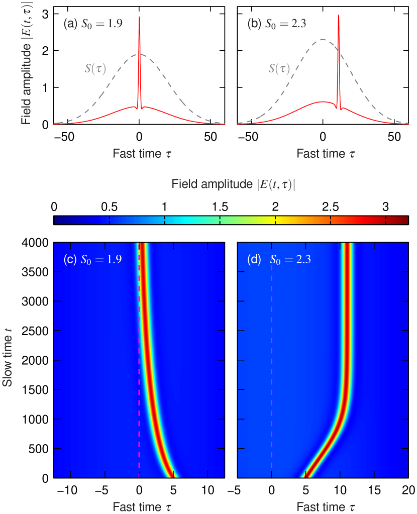
Figure 1: (a,b) Steady-state intracavity field solutions (red curves) for peak driving amplitudes (a) $S_{0}=1.9$ and (b) $S_{0}=2.3$. Gray dashed curves show the corresponding Gaussian driving field profiles. (c,d) Dynamical intracavity field evolutions corresponding to (a) and (b), respectively. The initial soliton position $\tau_{0}=5$. Dashed vertical magenta line highlights the position of the maximum driving field amplitude ($\tau=0$). Note the different $x$-axes in (c) and (d).

Figures 1(a) and (b) show steady-state field profiles obtained for a constant detuning $\Delta=4$ but for two different driving field amplitudes $S_{0}=1.9$ and $S_{0}=2.3$, respectively. Corresponding dynamical evolutions of the intracavity fields are shown as the false colour plots in Figs 1(c) and (d). As can be seen, for $S_{0}=1.9$ the CS is attracted to the peak of the driving field amplitude at $\tau=0$. In contrast, for $S_{0}=2.3$, the CS drifts down along the driving pulse profile, eventually stabilizing at $\tau_{\mathrm{CS}}\approx 11.0$ where $S(\tau_{\mathrm{CS}})\approx 1.98$. Additional simulations (not shown here) reveal that, if the CS is initially excited slightly below the observed trapping point ($\tau_{0}>\tau_{\mathrm{CS}}$), it will move up along the driving pulse profile until it again stabilizes at $\tau_{\mathrm{CS}}\approx 11.0$. Moreover, if the soliton is initially excited at $\tau_{0}<0$, it will be attracted towards $\tau_{\mathrm{CS}}\approx-11.0$ where $S(\tau_{\mathrm{CS}})\approx 1.98$. This clearly shows that, as expected based on symmetry considerations, the sign of the intensity gradient of the driving field plays no role in determining the CS’s equilibrium position.

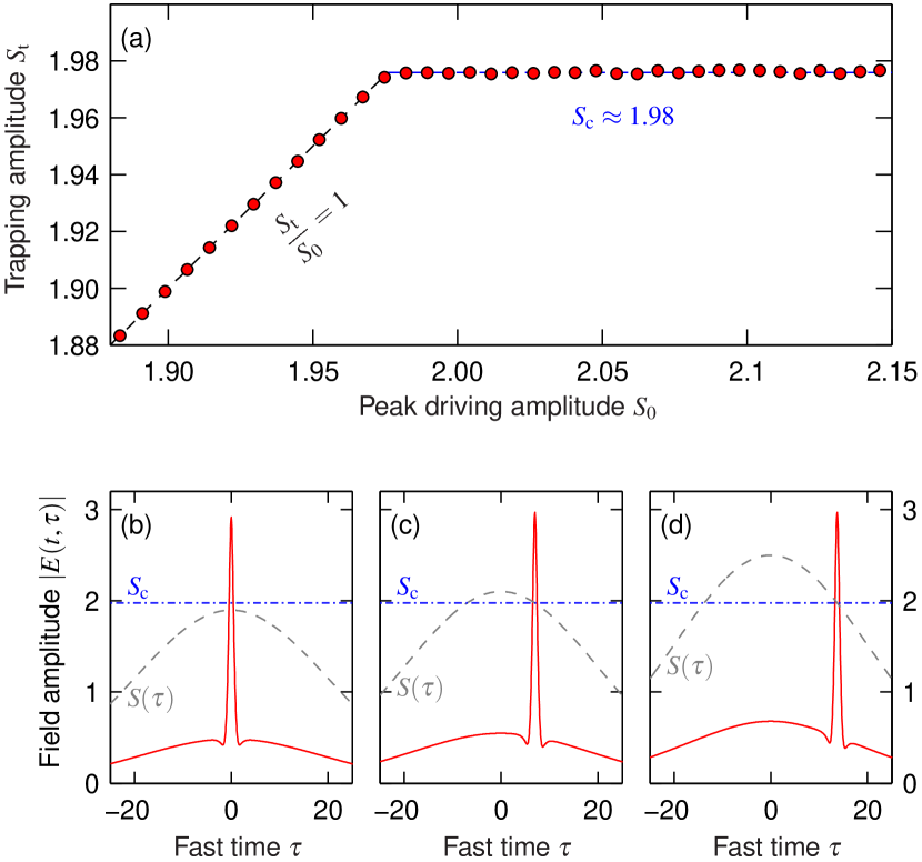
Figure 2: (a) Driving field amplitude at the steady-state CS position [$S_{\mathrm{t}}=S(\tau_{\mathrm{CS}})$] as a function of the peak driving amplitude $S_{0}$. (b)–(d) Red curves show steady-state intracavity field profiles for three different driving amplitudes: (b) $S_{0}=1.9$, (c) $S_{0}=2.1$, and (d) $S_{0}=2.5$. Gray dashed curves show the corresponding Gaussian driving field profiles $S(\tau)$. Dash-dotted horizontal blue line indicates the critical driving value $S_{\mathrm{c}}=1.98$. A detuning $\Delta=4$ was used in all calculations.

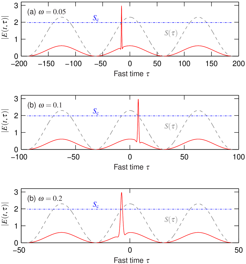
Figure 3: Steady-state field profiles (red curves) for a co-sinusoidal driving field with different modulation frequencies as indicated. The CSs were initially excited at (a) $\tau_{0}=-1$, (b) $\tau_{0}=1$, and (c) $\tau_{0}=-1$. Gray dashed curves show the corresponding driving field profiles, while the dash-dotted horizontal blue curve highlights $S_{\mathrm{c}}\approx 1.98$. All calculations use $S_{0}=2.3$ and $\Delta=4$. Note the different fast time axes in (a)–(c).

To gain more insights, we repeated the simulations above for a range of driving pulse amplitudes $S_{0}$. For each simulation, we extracted the final position $\tau_{\mathrm{CS}}$ of the CS relative to the peak of the driving pulse (at $\tau=0$), as well as the corresponding value of the driving field at this point, i.e., $S_{\mathrm{t}}=S(\tau_{\mathrm{CS}})$. In Fig. 2, we plot $S_{\mathrm{t}}$ as a function of the peak driving amplitude $S_{0}$. For small $S_{0}$, we find $S_{\mathrm{t}}=S_{0}$: the CS is attracted and trapped to the peak of the driving field. However, when the peak driving amplitude increases beyond a critical value $S_{\mathrm{c}}\approx 1.98$, the soliton is always found to drift to a position with that driving field value. This behaviour is illustrated in Figs 2(b)–(d), where we plot the steady-state field profiles corresponding to three different driving peak amplitudes (see caption). In Fig. 2(b), the peak driving amplitude $S_{0}<S_{\mathrm{c}}$, and so the CS is attracted to the maximum of the driving profile. In contrast, in Figs. 2(c) and (d), the driving field encompasses the critical value $S_{\mathrm{c}}$, causing the CS to be trapped at one of the positions where $S(\tau_{\mathrm{CS}})=S_{\mathrm{c}}$. We again emphasize that, depending on the initial condition, the CS can be trapped on either side of the Gaussian where $S(\tau)=S_{\mathrm{c}}$.

The results above suggest that Kerr CSs are attracted to positions where the driving field attains the critical value $S_{\mathrm{c}}$. It is only when the maximum driving amplitude is less than that critical value [as in Fig. 2(b)] that the soliton stabilizes at a maximum of the driving field. (Conversely, if the minimum of the driving amplitude is larger than the critical value, the soliton will be trapped at the minimum of the driving field.) Similar behaviour has previously been attributed to CSs of quadratically nonlinear resonators fedorov_effects_2001 . Through extensive simulations, we have found that the critical trapping level $S_{\mathrm{c}}$ does not depend on the driving field profile or on the amplitude gradient at the trapping point. To illustrate this, we consider a sinusoidally amplitude modulated driving field of the form

$$S(\tau)=\frac{S_{0}}{2}\left[1+\cos(\omega\tau)\right].$$ (3)

Figures 3(a)–(c) show steady-state profiles for three different modulation frequencies $\omega$ (see caption) with the peak driving amplitude and detuning held constant [at $S_{0}=2.3$ and $\Delta=4$ as in Fig. 1(b)]. Here, to illustrate how the solitons can be trapped both at the rising or the falling edge of the driving field, different initial positions $\tau_{0}$ were used [see caption]. Despite the differences in driving field gradients ($S^{\prime}(\tau_{\mathrm{CS}})\propto\omega$), in each case the CS is found to trap at a position where $S(\tau_{\mathrm{CS}})\approx 1.98$, which coincides with the value found for pulsed driving in Fig. 1(b).

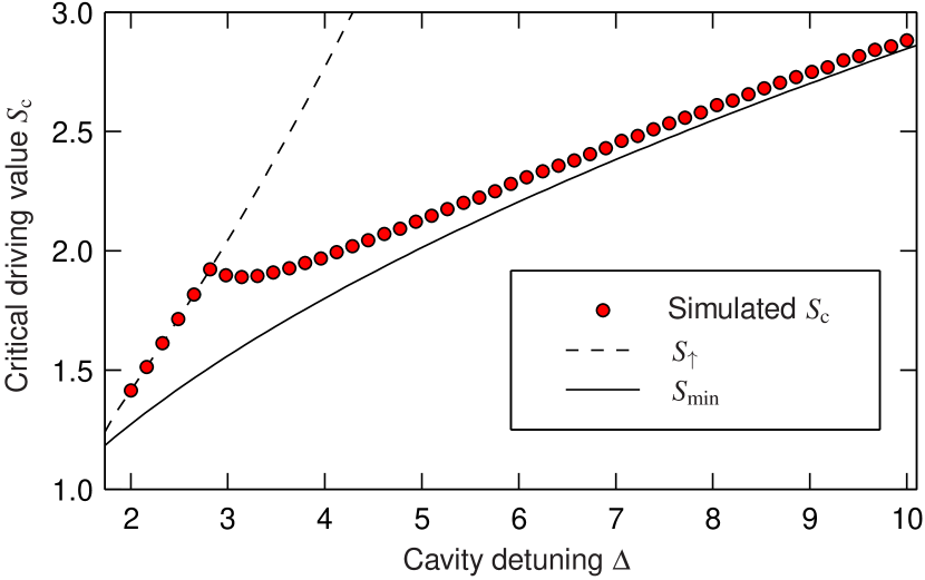
Figure 4: Critical driving field values $S_{\mathrm{c}}$ as a function of detuning. Red solid circles correspond to values extracted from numerical simulations, while solid black curve highlights the minimum driving amplitude needed for CS existence: $S_{\mathrm{min}}=(8\Delta/\pi^{2})^{1/2}$. Dashed black curve highlights the up-switching point $S_{\uparrow}=[2/27(\Delta^{3}+9\Delta+\sqrt{\Delta^{2}-3})]^{1/2}$, above which the homogeneous response of the LLE is monostable. CSs can exist between the dashed and solid curves.

Whilst the critical driving amplitude $S_{\mathrm{c}}$ does not depend on the overall driving field profile, it does depend on the cavity detuning $\Delta$. We repeated the simulations above for a range of detunings, and extracted the driving field value towards which the CSs are attracted to. To ensure that the peak driving amplitude $S_{0}$ is sufficiently large to capture the critical value $S_{\mathrm{c}}$, we used a Gaussian driving profile with amplitude $S_{0}=S_{\uparrow}=[2/27(\Delta^{3}+9\Delta+\sqrt{\Delta^{2}-3})]^{1/2}$. (This amplitude corresponds to the upper limit of the homogeneous bistability cycle of Eq. (1), and hence the absolute upper limit of CS existence leo_temporal_2010 .) In Fig. 4, we plot the critical driving value $S_{\mathrm{c}}$ obtained from our simulations as a function of the cavity detuning $\Delta$. Also shown are the maximum ($S_{\uparrow}$, dashed line) and minimum ($S_{\mathrm{min}}=(8\Delta/\pi^{2})^{1/2}$, solid line) driving field amplitudes between which CSs can exist leo_dynamics_2013 ; herr_temporal_2014 ; barashenkov_existence_1996 . Two different regimes showing qualitatively different behaviour can be identified. For small $\Delta\lesssim 2.9$, we find $S_{\mathrm{c}}\approx S_{\uparrow}$: in this regime, a CS will always be attracted towards the local maximum of the driving field ($S_{0}$). In contrast, for larger $\Delta$, the trapping level $S_{\mathrm{c}}$ approaches the minimum driving field amplitude $S_{\mathrm{min}}$. In this regime, the CS can be trapped at the edge of the driving field profile, and in the limit of $\Delta\gg 1$, drift to the lowest possible value of $S$ for which it can still exist. This latter behaviour is similar to the dynamics observed in quadratically nonlinear systems fedorov_effects_2001 , where soliton motion was explained by their tendency to approach conditions of nonlinear resonance. Indeed, we find that, for a given detuning $\Delta$, our Kerr CSs reach their maximum amplitude and they are precisely in-phase with the driving field when $S\approx(8\Delta/\pi^{2})^{1/2}\approx S_{\mathrm{min}}$, thus evidencing the realization of resonance conditions.

The observation that, for $\Delta\gtrsim 2.9$, Kerr CSs can be trapped at the edge of the driving field profile is amenable to an interpretation in terms of a spontaneous symmetry breaking instability xu_experimental_2014 . This can be readily seen by plotting the possible steady-state CS positions, $\tau_{\mathrm{CS}}$, as a function of the peak driving strength $S_{0}$. An example of such a bifurcation curve is shown in Fig. 5; the steady-state field profiles were obtained using a Newton-Raphson continuation algorithm with a Gaussian driving field and $\Delta=4$. For small $S_{0}$, the CSs sit stably atop the driving field maximum [c.f. Fig. 2(b)], and there is accordingly only a single steady-state configuration (with $\tau_{\mathrm{CS}}=0$, blue curves). However, as $S_{0}$ increases past the critical level $S_{\mathrm{c}}$, a clear pitchfork bifurcation can be observed Bruno : the symmetric state with a CS at $\tau_{\mathrm{CS}}=0$ becomes unstable, and a pair of new asymmetric stable states emerge that consist of a CS sitting on either side of the driving field maximum [red curves; see also Figs 2(c) and (d)].

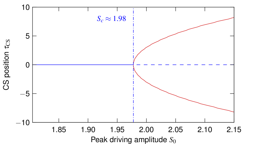
Figure 5: CS symmetry breaking bifurcation curve for a Gaussian driving field with $\tau_{\mathrm{G}}=20$ and $\Delta=4$. Blue and red curves show the steady-state positions of the CS solutions as a function of the maximum driving amplitude for symmetric and asymmetric states, respectively, with the dashed part being unstable. Dash-dotted vertical line indicates the critical driving value $S_{\mathrm{c}}$.

It is somewhat surprising that Kerr CSs can be trapped at a position where the driving field amplitude gradient is non-zero. Indeed, to first order, the CS’s drift velocity can be shown to be directly proportional to that gradient  maggipinto_cavity_2000 ; javaloyes_dynamics_2016 :

$$v=\frac{d\tau_{\mathrm{CS}}}{dt}=a\left.\frac{dS}{d\tau}\right|_{\tau=\tau_{\mathrm{CS}}},$$ (4)

where the proportionality coefficient $a$ describes the projection of the CS’s neutral (or Goldstone) mode along a linear fast time variation. Note that amplitude modulations correspond to purely real perturbations and only couple to the real part of the neutral mode, in stark contrast to phase modulations. Accordingly, while Eq. (4) holds true also for the case of phase modulated driving fields, the coefficient $a$ differs between the two forms of perturbations  maggipinto_cavity_2000 .

The apparent discrepancy between our findings and Eq. (4) is explained by the fact that the CS’s neutral mode changes with the driving strength (and detuning). As a consequence (and similarly to quadratically nonlinear systems fedorov_effects_2001 ), the proportionality coefficient $a$ in Eq. (4) also depends on the driving strength (and detuning), i.e., $a=a(S_{\mathrm{H}},\Delta)$, where $S_{\mathrm{H}}=S(\tau_{\mathrm{CS}})$. This is illustrated in Fig. 6, where we explicitly show $a(S_{\mathrm{H}},\Delta)$ computed for a range of cavity driving strengths and detunings maggipinto_cavity_2000 . These results were obtained by first finding the steady-state CS solutions of Eq. (1) for a homogeneous driving field with strength $S_{\mathrm{H}}$ and detuning $\Delta$, and then projecting the real part of the solitons’ neutral mode (technically the odd components of the left eigenvector with zero eigenvalue of the system’s Jacobian) along a linear fast time variation maggipinto_cavity_2000 .

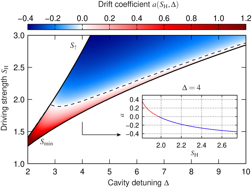
Figure 6: Drift coefficient $a(S_{\mathrm{H}},\Delta)$ calculated from the neutral mode of a steady-state CS solution for a range of homogeneous driving strengths $S_{\mathrm{H}}$ and cavity detunings $\Delta$. The solid black curves correspond to $S_{\mathrm{min}}$ and $S_{\uparrow}$ as defined in the caption of Fig. 4; CSs only exist between these two curves. Black dashed curve shows the critical driving field values $S_{\mathrm{c}}$ obtained from direct numerical simulations of the LLE with a Gaussian driving field [same data is shown in Fig. 4]. Inset shows the curve $a(S_{\mathrm{H}},\Delta=4)$.

As can be seen, the coefficient $a$ decreases with increasing driving strength, and for $\Delta\gtrsim 2.9$, crosses zero within the region of CS existence. Moreover, we see that the curve $a(S_{\mathrm{H}},\Delta)=0$ matches exactly with the critical driving field values found through direct split-step simulations of Eq. (1) with an inhomogeneous driving field [c.f. Fig. 4]. These findings fully corroborate our observations of CS behaviour in the presence of driving field amplitude inhomogeneities. Specifically, when a CS drifts along an amplitude gradient, the coefficient $a$ it experiences changes continuously. At the critical level $S_{\mathrm{c}}$, the coefficient passes through zero and changes sign, thus enabling robust trapping at that level. On the other hand, whilst the maximum (or minimum) of the driving field (with $dS/d\tau=0$) always corresponds to an equilibrium position, that equilibrium position is unstable [c.f. Fig. 5] if the maximum (minimum) is larger (smaller) than the critical driving value $S_{\mathrm{c}}$. There is therefore no contradiction between our findings and Eq. (4): the soliton velocity is “locally” proportional to the driving field gradient [as described by Eq. (4)], but because the proportionality coefficient changes as the soliton drifts, the overall relationship is more complex. (Rigorously speaking, the soliton velocity is proportional to the driving field gradient only over short slow time intervals during which the “local” driving strength — and hence the coefficient $a(S_{\mathrm{H}},\Delta$) — experienced by the soliton remains approximately constant.) It is also worth highlighting that, because the drift coefficient $a(S_{\mathrm{H}},\Delta)$ only depends on the local value of the driving field ($S_{\mathrm{H}}$) and the detuning, the analysis above readily explains why the critical trapping level $S_{\mathrm{c}}$ does not depend on the precise profile of the driving field (provided that the driving field varies slowly compared to the CS duration).

To better understand the physics that underpins the Kerr CS behaviour identified above, we next present results from simulations of an Ikeda-like map ikeda_multiple-valued_1979 . Unlike the mean-field approximation of Eq. (1), this approach allows us to isolate effects due to (i) propagation through the Kerr medium over a single cavity round trip and (ii) the coherent injection of the driving field into the cavity. We write the map equations in dimensionless form with units that allow immediate comparison with results from Eq. (1):

$$\frac{\partial E_{m}(\xi,\tau)}{\partial\xi} =i\frac{\partial^{2}E_{m}}{\partial\tau^{2}}+i|E_{m}|^{2}E_{m},$$ (5)

$$E_{m+1}(\xi=0,\tau) =\sqrt{1-2\alpha}\,E_{m}(\xi=\alpha,\tau)e^{-i\delta_{0}}+\alpha S(\tau).$$ (6)

Here, Eq. (5) is the well-known nonlinear Schrödinger equation (NLSE) that describes the evolution of the intracavity field over one cavity round trip, with $\xi=\alpha z/L$ a dimensionless propagation coordinate ($z$ is the corresponding dimensional variable), while Eq. (6) is the boundary condition that describes the addition of the coherent driving field to the intracavity light field at $\xi=0$. For high-finesse cavities, $\alpha\ll 1$, and the above map equations can be averaged to the LLE given by Eq. (1). To better capture the evolution of the soliton over one cavity round trip, we have used a comparatively large value of $\alpha=0.15$ in the simulations that will follow.

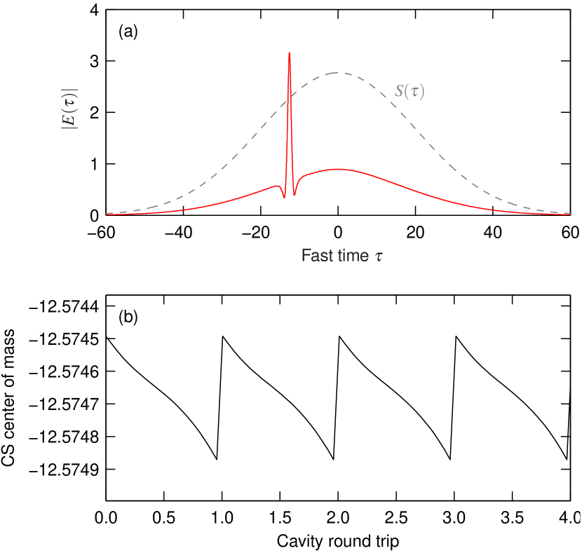
Figure 7: Simulation results from an Ikeda-like cavity map. (a) Steady-state intracavity field profile (red curve) for a Gaussian driving field (gray dashed curve). (b) Evolution of the CS’s center of mass over four cavity transits.

Figure 7(a) shows a steady-state intracavity field obtained from the Ikeda map with $\Delta=4$ and a Gaussian driving field profile with $S_{0}=S_{\uparrow}\approx 2.77$ and $\tau_{\mathrm{G}}=20$. One first notes that the Ikeda map reproduces the salient result of the LLE simulation, i.e., the CS trapping at a position where the driving field gradient is non-zero. The precise trapping value $S_{\mathrm{c}}\approx 2.27$ is somewhat larger than the value found in corresponding mean-field simulations, which we attribute to the comparatively large value of $\alpha$. Indeed, we have carefully verified that the Ikeda map reproduces the LLE result in the limit of very small $\alpha$.

To gain insights on the interplay between propagation over one round trip [described by Eq. (5)] and addition of the coherent driving [Eq. (6)], Fig. 7(b) shows the evolution of the CS’s centre of mass in the fast time dimension (calculated over the soliton’s half-maximum points) over four consecutive round trips after steady-state is reached. As can be seen, the CS drifts gently downwards away from the driving field maximum during propagation, but is pulled back to its original position at the boundary. This competition between propagation and coherent driving underpins the behaviour of CSs in the presence of pulsed or amplitude modulated driving fields. Specifically, if the propagation effect is stronger (weaker) than the driving effect, the coefficient $a$ in Eq. (4) is negative (positive), such that the CS will drift away from (towards) the maximum. In contrast, at the critical driving strength $S_{\mathrm{c}}$, the two effects are precisely balanced.

The physics behind the two competing effects identified above can be qualitatively explained as follows. First, the addition of the driving field can be intuitively understood to shift the CS towards its maximum because the two are almost in-phase. In contrast, the soliton’s drift away from the maximum during propagation is due to the phase shift between the soliton and the intracavity background field. Considering a superposition field $E(\xi,\tau)=E_{\mathrm{s}}(\xi,\tau)+\delta E(\xi,\tau)$ that consists of an NLSE soliton ($E_{\mathrm{s}}$) perturbed by a small amplitude background field ($\delta E$), it is well known that the perturbation can cause the soliton to drift, with the rate of drift given by the inverse group velocity gordon_random_1986

$$\frac{\Delta\tau_{\mathrm{S}}}{\Delta\xi}=-\frac{1}{A}\mathrm{Im}\int\frac{\partial E_{\mathrm{s}}^{*}}{\partial\tau}\delta E\,\mathrm{d}t,$$ (7)

where $\Delta\tau_{\mathrm{S}}$ and $A$ represent the soliton’s temporal position and amplitude, respectively. Straightforward analysis of Eq. (7) confirms that, when $\Delta\phi=\phi_{\mathrm{S}}-\phi_{\mathrm{\delta}}\in[0,\pi]$, where $\phi_{\mathrm{S}}$ and $\phi_{\mathrm{\delta}}$ denote respectively the phases of the soliton and the background, the soliton will drift away from the perturbation maximum while the opposite is true for $\Delta\phi>\pi$. (We have also confirmed these predictions by means of direct numerical simulations of the NLSE Eq. (5).) For Kerr CSs, the two phases are approximately (in the mean-field limit) given by wabnitz_suppression_1993 ; herr_temporal_2014

$$\phi_{\mathrm{S}} \approx\cos^{-1}\left(\frac{\sqrt{8\Delta}}{\pi S}\right),$$ (8)

$$\phi_{\mathrm{\delta}} \approx-\tan^{-1}\left(\Delta\right).$$ (9)

As CSs exist only for $\Delta>0$, one always finds $\Delta\phi\in[0,\pi]$, explaining the soliton’s downward motion over a single cavity round trip. It is worth noting that, if the soliton sits at an extremum of the driving field (where ${\partial E_{\mathrm{s}}^{*}/\partial\tau=0}$), this motion vanishes [see Eq. 7]. Because the addition of a parity symmetric driving field will likewise induce no shifts in this situation, we can see how the driving field extrema indeed correspond to equilibria, whose stability is governed by the relative strengths of the two competing effects.

To conclude, we have investigated the dynamics of Kerr CSs in the presence of driving fields with inhomogeneous amplitude profiles. In stark contrast to the case of phase inhomogeneities, we have shown that the CSs are not in general attracted to maxima (or minima) of an amplitude modulated driving field. Instead, the solitons are attracted to — and trap to — positions associated with particular values of the driving field. We have described the underlying physics in terms of a spontaneous symmetry breaking instability that arises from a competition between the coherent addition of the driving field and propagation in the Kerr medium.

Our work complements previous studies of symmetry breaking in Kerr cavities garcia-mateos_optical_1995 ; torres_bilateral_1999 ; schmidberger_multistability_2014 ; xu_experimental_2014 ; rossi_spontaneous_2016 ; cao_experimental_2017 ; bino_symmetry_2017 , and raises several interesting questions for follow-up research: how do CSs behave in presence of amplitude and phase inhomogeneities; does the universality of the general behavior evoked by amplitude inhomogeneities extend beyond Kerr cavities and the quadratically nonlinear systems studied in fedorov_effects_2001 ? Of course, experimentally verifying the predictions outlined in our current work also represents a significant future contribution. While some of us have already observed experimental evidence of CS trapping to the edge of a nanosecond pump pulse wang_intensity_2017 , the results obtained do not allow unequivocal discrimination between effects arising from intrinsic cavity dynamics and non-ideal driving conditions (e.g. synchronization mismatch or residual pump phase modulation). On the other hand, clean experimental evidence of symmetry breaking has previously been observed in a fiber ring resonator driven with pulses from a mode-locked laser xu_experimental_2014 . Although that study did not explore the connection between symmetry breaking and CS trapping, we believe that the experimental configuration used could allow for the controlled examination of the behaviours identified in our current work.

- (1) S. Wabnitz, “Suppression of interactions in a phase-locked soliton optical memory,” Optics Letters 18, 601–603 (1993).
- (2) F. Leo, S. Coen, P. Kockaert, S.-P. Gorza, P. Emplit, and M. Haelterman, “Temporal cavity solitons in one-dimensional Kerr media as bits in an all-optical buffer,” Nature Photonics 4, 471–476 (2010).
- (3) F. Leo, L. Gelens, P. Emplit, M. Haelterman, and S. Coen, “Dynamics of one-dimensional Kerr cavity solitons,” Optics Express 21, 9180–9191 (2013).
- (4) J. K. Jang, M. Erkintalo, S. G. Murdoch, and S. Coen, “Ultraweak long-range interactions of solitons observed over astronomical distances,” Nature Photonics 7, 657–663 (2013).
- (5) J. K. Jang, M. Erkintalo, S. G. Murdoch, and S. Coen, “Observation of dispersive wave emission by temporal cavity solitons,” Optics Letters 39, 5503–5506 (2014).
- (6) J. K. Jang, M. Erkintalo, S. Coen, and S. G. Murdoch, “Temporal tweezing of light through the trapping and manipulation of temporal cavity solitons,” Nature Communications 6 (2015).
- (7) K. Luo, J. K. Jang, S. Coen, S. G. Murdoch, and M. Erkintalo, “Spontaneous creation and annihilation of temporal cavity solitons in a coherently driven passive fiber resonator,” Optics Letters 40, 3735–3738 (2015).
- (8) M. Anderson, F. Leo, S. Coen, M. Erkintalo, and S. G. Murdoch, “Observations of spatiotemporal instabilities of temporal cavity solitons,” Optica 3, 1071–1074 (2016).
- (9) J. K. Jang, M. Erkintalo, J. Schröder, B. J. Eggleton, S. G. Murdoch, and S. Coen, “All-optical buffer based on temporal cavity solitons operating at 10 Gb/s,” Optics Letters 41, 4526–4529 (2016).
- (10) T. Herr, V. Brasch, J. D. Jost, C. Y. Wang, N. M. Kondratiev, M. L. Gorodetsky, and T. J. Kippenberg, “Temporal solitons in optical microresonators,” Nature Photonics 8, 145–152 (2014).
- (11) S. Coen, H. G. Randle, T. Sylvestre, and M. Erkintalo, “Modeling of octave-spanning Kerr frequency combs using a generalized mean-field Lugiato–Lefever model,” Optics Letters 38, 37–39 (2013).
- (12) Y. K. Chembo and C. R. Menyuk, “Spatiotemporal Lugiato-Lefever formalism for Kerr-comb generation in whispering-gallery-mode resonators,” Physical Review A 87, 053852 (2013).
- (13) P. Parra-Rivas, D. Gomila, M. A. Matías, S. Coen, and L. Gelens, “Dynamics of localized and patterned structures in the Lugiato-Lefever equation determine the stability and shape of optical frequency combs,” Physical Review A 89, 043813 (2014).
- (14) X. Yi, Q.-F. Yang, K. Y. Yang, M.-G. Suh, and K. Vahala, “Soliton frequency comb at microwave rates in a high-Q silica microresonator,” Optica 2, 1078–1085 (2015).
- (15) V. Brasch, M. Geiselmann, T. Herr, G. Lihachev, M. H. P. Pfeiffer, M. L. Gorodetsky, and T. J. Kippenberg, “Photonic chip–based optical frequency comb using soliton Cherenkov radiation,” Science 351, 357–360 (2016).
- (16) C. Joshi, J. K. Jang, K. Luke, X. Ji, S. A. Miller, A. Klenner, Y. Okawachi, M. Lipson, and A. L. Gaeta, “Thermally controlled comb generation and soliton modelocking in microresonators,” Optics Letters 41, 2565–2568 (2016).
- (17) K. E. Webb, M. Erkintalo, S. Coen, and S. G. Murdoch, “Experimental observation of coherent cavity soliton frequency combs in silica microspheres,” Optics Letters 41, 4613–4616 (2016).
- (18) P. Marin-Palomo, J. N. Kemal, M. Karpov, A. Kordts, J. Pfeifle, M. H. P. Pfeiffer, P. Trocha, S. Wolf, V. Brasch, M. H. Anderson, R. Rosenberger, K. Vijayan, W. Freude, T. J. Kippenberg, and C. Koos, “Microresonator-based solitons for massively parallel coherent optical communications,” Nature 546, 274–279 (2017).
- (19) X. Yi, Q.-F. Yang, X. Zhang, K. Y. Yang, X. Li, and K. Vahala, “Single-mode dispersive waves and soliton microcomb dynamics,” Nature Communications 8, 14869 (2017).
- (20) A. M. Weiner, “Frequency combs: Cavity solitons come of age,” Nature Photonics 11, 533–535 (2017).
- (21) V. Brasch, E. Lucas, J. D. Jost, M. Geiselmann, and T. J. Kippenberg, “Self-referenced photonic chip soliton Kerr frequency comb,” Light: Science & Applications 6, e16202 (2017).
- (22) M. H. P. Pfeiffer, C. Herkommer, J. Liu, H. Guo, M. Karpov, E. Lucas, M. Zervas, and T. J. Kippenberg, “Octave-spanning dissipative Kerr soliton frequency combs in SiN microresonators,” Optica 4, 684–691 (2017).
- (23) X. Xue, X. Zheng, and A. M. Weiner, “Soliton trapping and comb self-referencing in a single microresonator with and nonlinearities,” Optics Letters 42, 4147–4150 (2017).
- (24) A. Pasquazi, M. Peccianti, L. Razzari, D. J. Moss, S. Coen, M. Erkintalo, Y. K. Chembo, T. Hansson, S. Wabnitz, P. Del’Haye, X. Xue, A. M. Weiner, and R. Morandotti, “Micro-combs: A novel generation of optical sources,” Physics Reports 729, 1–81 (2017).
- (25) T. Ackemann, W. Firth, and G. Oppo, “Chapter 6 Fundamentals and Applications of Spatial Dissipative Solitons in Photonic Devices,” in P. R. B. a. C. C. L. E. Arimondo, editor, “Advances In Atomic, Molecular, and Optical Physics,” Volume 57 of Advances in Atomic Molecular and Optical Physics, pages 323–421, Academic Press (2009).
- (26) S. Barland, J. R. Tredicce, M. Brambilla, L. A. Lugiato, S. Balle, M. Giudici, T. Maggipinto, L. Spinelli, G. Tissoni, T. Knödl, M. Miller, and R. Jäger, “Cavity solitons as pixels in semiconductor microcavities,” Nature 419, 699–702 (2002).
- (27) S. Barland, S. Coen, M. Erkintalo, M. Giudici, J. Javaloyes, and S. Murdoch, “Temporal localized structures in optical resonators,” Advances in Physics: X 2, 496–517 (2017).
- (28) Y. Wang, F. Leo, J. Fatome, M. Erkintalo, S. G. Murdoch, and S. Coen, “Universal mechanism for the binding of temporal cavity solitons,” Optica 4, 855–863 (2017).
- (29) P. Parra-Rivas, D. Gomila, P. Colet, and L. Gelens, “Interaction of solitons and the formation of bound states in the generalized Lugiato-Lefever equation,” The European Physical Journal D 71, 198 (2017).
- (30) D. C. Cole, E. S. Lamb, P. Del’Haye, S. A. Diddams, and S. B. Papp, “Soliton crystals in Kerr resonators,” Nature Photonics 11, 671–676 (2017).
- (31) W. J. Firth and A. J. Scroggie, “Optical Bullet Holes: Robust Controllable Localized States of a Nonlinear Cavity,” Physical Review Letters 76, 1623–1626 (1996).
- (32) T. Maggipinto, M. Brambilla, G. K. Harkness, and W. J. Firth, “Cavity solitons in semiconductor microresonators: Existence, stability, and dynamical properties,” Physical Review E 62, 8726–8739 (2000).
- (33) F. Pedaci, S. Barland, E. Caboche, P. Genevet, M. Giudici, J. R. Tredicce, T. Ackemann, A. J. Scroggie, W. J. Firth, G.-L. Oppo, G. Tissoni, and R. Jäger, “All-optical delay line using semiconductor cavity solitons,” Applied Physics Letters 92, 011101–011101–3 (2008).
- (34) F. Pedaci, P. Genevet, S. Barland, M. Giudici, and J. R. Tredicce, “Positioning cavity solitons with a phase mask,” Applied Physics Letters 89, 221111 (2006).
- (35) J. K. Jang, M. Erkintalo, K. Luo, G.-L. Oppo, S. Coen, and S. G. Murdoch, “Controlled merging and annihilation of localised dissipative structures in an AC-driven damped nonlinear Schrödinger system,” New Journal of Physics 18, 033034 (2016).
- (36) G. Steinmeyer, A. Buchholz, M. Hänsel, M. Heuer, A. Schwache, and F. Mitschke, “Dynamical pulse shaping in a nonlinear resonator,” Physical Review A 52, 830–838 (1995).
- (37) F. Mitschke and A. Schwache, “Soliton ensembles in a nonlinear resonator,” Quantum and Semiclassical Optics: Journal of the European Optical Society Part B 10, 779–788 (1998).
- (38) J. García-Mateos, F. C. Bienzobas, and M. Haelterman, “Optical bistability and temporal symmetry-breaking instability in nonlinear fiber resonators,” Fiber and Integrated Optics 14, 337–346 (1995).
- (39) J. P. Torres, J. Boyce, and R. Y. Chiao, “Bilateral Symmetry Breaking in a Nonlinear Fabry-Pérot Cavity Exhibiting Optical Tristability,” Physical Review Letters 83, 4293–4296 (1999).
- (40) Y. Xu and S. Coen, “Experimental observation of the spontaneous breaking of the time-reversal symmetry in a synchronously pumped passive Kerr resonator,” Optics Letters 39, 3492–3495 (2014).
- (41) M. J. Schmidberger, D. Novoa, F. Biancalana, P. S. J. Russell, and N. Y. Joly, “Multistability and spontaneous breaking in pulse-shape symmetry in fiber ring cavities,” Optics Express 22, 3045–3053 (2014).
- (42) P. Parra-Rivas, D. Gomila, M. A. Matías, P. Colet, and L. Gelens, “Effects of inhomogeneities and drift on the dynamics of temporal solitons in fiber cavities and microresonators,” Optics Express 22, 30943–30954 (2014).
- (43) T. Hansson and S. Wabnitz, “Bichromatically pumped microresonator frequency combs,” Physical Review A 90, 013811 (2014).
- (44) W. B. Cardoso, L. Salasnich, and B. A. Malomed, “Localized solutions of Lugiato-Lefever equations with focused pump,” Scientific Reports 7, 16876 (2017).
- (45) M. Malinowski, A. Rao, P. Delfyett, and S. Fathpour, “Optical frequency comb generation by pulsed pumping,” APL Photonics 2, 066101 (2017).
- (46) L. A. Lugiato and R. Lefever, “Spatial Dissipative Structures in Passive Optical Systems,” Physical Review Letters 58, 2209–2211 (1987).
- (47) M. Anderson, Y. Wang, F. Leo, S. Coen, M. Erkintalo, and S. G. Murdoch, “Coexistence of Multiple Nonlinear States in a Tristable Passive Kerr Resonator,” Physical Review X 7, 031031 (2017).
- (48) E. Obrzud, S. Lecomte, and T. Herr, “Temporal solitons in microresonators driven by optical pulses,” Nature Photonics 11, 600–607 (2017).
- (49) J. Javaloyes, P. Camelin, M. Marconi, and M. Giudici, “Dynamics of Localized Structures in Systems with Broken Parity Symmetry,” Physical Review Letters 116, 133901 (2016).
- (50) P. Camelin, J. Javaloyes, M. Marconi, and M. Giudici, “Electrical addressing and temporal tweezing of localized pulses in passively-mode-locked semiconductor lasers,” Physical Review A 94, 063854 (2016).
- (51) J. Rossi, R. Carretero-González, P. G. Kevrekidis, and M. Haragus, “On the spontaneous time-reversal symmetry breaking in synchronously-pumped passive Kerr resonators,” Journal of Physics A: Mathematical and Theoretical 49, 455201 (2016).
- (52) Q.-T. Cao, H. Wang, C.-H. Dong, H. Jing, R.-S. Liu, X. Chen, L. Ge, Q. Gong, and Y.-F. Xiao, “Experimental Demonstration of Spontaneous Chirality in a Nonlinear Microresonator,” Physical Review Letters 118, 033901 (2017).
- (53) L. Del Bino, J. M. Silver, S. L. Stebbings, and P. Del’Haye, “Symmetry Breaking of Counter-Propagating Light in a Nonlinear Resonator,” Scientific Reports 7, 43142 (2017).
- (54) A. J. Scroggie, J. Jeffers, G. McCartney, and G.-L. Oppo, “Reversible soliton motion,” Physical Review E 71, 046602 (2005).
- (55) S. Fedorov, D. Michaelis, U. Peschel, C. Etrich, D. V. Skryabin, N. Rosanov, and F. Lederer, “Effects of spatial inhomogeneities on the dynamics of cavity solitons in quadratically nonlinear media,” Physical Review E 64, 036610 (2001).
- (56) E. Obrzud, M. Rainer, A. Harutyunyan, M. H. Anderson, M. Geiselmann, B. Chazelas, S. Kundermann, S. Lecomte, M. Cecconi, A. Ghedina, E. Molinari, F. Pepe, F. Wildi, F. Bouchy, T. J. Kippenberg, and T. Herr, “A Microphotonic Astrocomb,” arXiv:1712.09526 [astro-ph, physics:physics] (2017).
- (57) M. Haelterman, S. Trillo, and S. Wabnitz, “Dissipative modulation instability in a nonlinear dispersive ring cavity,” Optics Communications 91, 401–407 (1992).
- (58) S. Coen, M. Tlidi, Ph. Emplit, and M. Haelterman,“Convection versus Dispersion in Optical Bistability,” Physical Review Letters 83, 2328 (1999).
- (59) S. Coen and M. Erkintalo, “Universal scaling laws of Kerr frequency combs,” Optics Letters 38, 1790–1792 (2013).
- (60) I. V. Barashenkov and Y. S. Smirnov, “Existence and stability chart for the ac-driven, damped nonlinear Schrödinger solitons,” Physical Review E 54, 5707–5725 (1996).
- (61) A. H. Nayfeh and B. Balachandran, Applied Nonlinear Dynamics: Analytical, Computational, and Experimental Methods (Wiley-VCH Verlag GmbH, 2007).
- (62) K. Ikeda, “Multiple-valued stationary state and its instability of the transmitted light by a ring cavity system,” Optics Communications 30, 257–261 (1979).
- (63) J. P. Gordon and H. A. Haus, “Random walk of coherently amplified solitons in optical fiber transmission,” Optics Letters 11, 665–667 (1986).
- (64) Y. Wang, B. Garbin, G.-L. Oppo, S. Coen, M. Erkintalo, and S. G. Murdoch, “Intensity trapping of temporal cavity solitons,” in “2017 European Conference on Lasers and Electro-Optics and European Quantum Electronics Conference (2017), paper CD_3_5,” page CD_3_5, Optical Society of America (2017).