Scalar fields as sources for wormholes and regular black holes

Kirill A. Bronnikov
VNIIMS, Ozyornaya ul. 46, Moscow 119361, Russia;
Institute of Gravitation and Cosmology, Peoples’ Friendship University of Russia (RUDN University),
      ul. Miklukho-Maklaya 6, Moscow 117198, Russia;
National Research Nuclear University “MEPhI”, Kashirskoe sh. 31, Moscow 115409, Russia

We review nonsingular static, spherically symmetric solutions of general relativity with minimally coupled scalar fields. Considered are wormholes and regular black holes (BHs) without a center, including black universes (BHs with expanding cosmology beyond the horizon). Such configurations require a “ghost” field with negative kinetic energy $K$. Ghosts can be invisible under usual conditions if $K<0$ only in strong-field region (“trapped ghost”), or they rapidly decay at large radii. Before discussing particular examples, some general results are presented, such as the necessity of anisotropic matter for asymptotically flat or AdS wormholes, no-hair and global structure theorems for BHs with scalar fields. The stability properties of scalar wormholes and regular BHs under spherical perturbations are discussed. It is stressed that the effective potential $V_{\rm eff}$ for perturbations has universal shapes near generic wormhole throats (a positive pole regularizable by a Darboux transformation) and near transition surfaces from canonical to ghost scalar field behavior (a negative pole at which the perturbation finiteness requirement plays a stabilizing role). Positive poles of $V_{\rm eff}$ emerging at “long throats” (with the radius $r\approx r_{0}+{\rm const}\cdot x^{2n}$, $n>1$, $x=0$ is the throat) may be regularized by repeated Darboux transformations for some values of $n$.

]

1 Introduction

Space-time singularities exist in a great number of solutions of general relativity (GR) with or without various material sources, and at each of them the theory itself demonstrates conditions under which it cannot work any more. However, construction of various nonsingular solutions of GR, which are especially interesting and attractive, is also a long-term tradition. In particular, nonsingular static, spherically symmetric space-times, which are a subject of this paper, may be classified as follows: (i) starlike (or solitonic, or particlelike) space-times with a regular center, (ii) black holes (BHs) with a regular center, (iii) space-times having no center and no horizons, including wormholes and some other geometries like horns and flux tubes, and (iv) space-times without a center but containing horizons, and among them are a few classes of regular BHs as well as wormholes with cosmological horizons — for reviews see, e.g., [1, 2, 3, 4, 5] and references therein. Our interest will be in wormholes and regular BHs (BHs) without a center described by solutions of GR with a minimally coupled scalar field as a source. Even such a narrow class of geometries turns out to be sufficiently rich in properties of interest, especially concerning their dynamic stability.

A wormhole is generally understood as a kind of tunnel or shortcut between two manifolds or two distant parts of the same manifold. However, this term is used in the literature in different meanings: the wormholes can be Lorentziian (traversable or not), Euclidean, and even quantum, which means that a wave function resembles a tunnel geometry in a certain sense. In this paper, the term “wormhole” is applied to traversable Lorentzian wormholes only. The so-called non-traversable wormholes are, in general, BHs (or parts of BH space-times) rather than wormholes; thus, a wormhole-like geometry quite usually appears as a spatial section of a black hole, and it is this phenomenon that was discovered by Flamm [6] as early as in 1916 in his study of Schwarzschild’s solution, and his article is now referred to as the pioneering paper in wormhole physics. As to Euclidean and quantum wormholes, they represent quite separate areas of research.

It is well known that the existence of traversable Lorentzian wormholes as solutions to the Einstein equations requires what is called “exotic matter”, i.e., matter violating the Null Energy Condition (NEC) [7, 8], which is a part of the Weak Energy Condition (WEC) whose physical meaning is that the energy density is nonnegative in any reference frame. In particular, for static, spherically symmetric systems sourced by scalar fields, wormhole solutions can be and are really obtained if such a scalar field is phantom (or ghost), i.e., has negative kinetic energy [9, 10, 11, 12]. In theories of gravity alternative to GR, for example, scalar-tensor theories and the related multidimensional and curvature-nonlinear theories, wormhole solutions also appear only in the presence of phantom degrees of freedom [9, 13, 14, 15] (see also [2, 3, 5] and references therein). This is true for both continuous matter distributions and thin shells [13]. In can happen that gravity itself becomes phantom in some region of space [9, 16, 13], in other cases the role of a phantom is played by such geometric quantities as torsion [17, 18], higher-dimensional metric components or variables related to higher-order derivatives [19, 20, 21] or unusual couplings between fields and matter [22]. For example, in brane-world theories, a source for wormhole geometry in four dimensions can be provided by a tidal effect from extra dimensions originating from the Weyl tensor in the bulk [21, 4, 23]. Such a source, due to its geometric origin, is not subject to any energy conditions applicable to ordinary matter.

If, however, our interest is in obtaining (at least potentially) realistic wormholes, it still makes sense to adhere to GR and to use macroscopic matter or fields, because it is GR that explains all observations and experiments on the macroscopic level; it is even used as a tool in applications like GPS navigation.

Still, as yet nobody has observed macroscopic phantom matter, which puts to doubt its possible existence and therefore a possible realization of wormholes, suitable, for instance, for interstellar communication and travel, even by any advanced civilization or in the remote future.

In attempts to circumvent such problems and still to find wormhole solutions in GR, a way of interest is to invoke such a sort of matter that would be phantom in a certain region of space only, somewhere in the vicinity of a wormhole throat, while away from it it would observe all usual energy conditions [24]. To obtain such a kind of matter, one can try to use a minimally coupled scalar field with the Lagrangian

$$L_{s}=h(\phi)g^{\mu\nu}\partial_{\mu}\phi\partial_{\nu}\phi-V(\phi),$$ (1)

where $h(\phi)$ and $V(\phi)$ are arbitrary functions. If $h(\phi)$ can change its sign, it cannot be absorbed by redefinition of $\phi$ in its whole range. A situation of interest for us is if $h>0$ (so that the scalar field is canonical and has positive kinetic energy) in a weak field region and $h<0$ (a phantom, or ghost scalar field) in a strong-field region where one could expect a wormhole throat. One can say that in this sense the ghost is trapped. Let us note that such a transition between $h>0$ and $h<0$ was considered in [25] in a cosmological setting.

It is known that phantom fields can produce not only wormholes but also regular black holes of different kinds, see, e.g., [26, 27, 28]. Among such models, it makes sense to mark separately those combining the features of BH physics and nonsingular cosmological models, the ones called black universes [26, 27]. Such objects look like “conventional” BHs (spherically symmetric ones in the existing examples) as seen from spatial infinity, where they can be asymptotically flat, but after crossing the horizon, a possible explorer gets into an expanding universe instead of a singularity. Thus such hypothetic objects combine the features of wormholes (no center but a regular minimum of the spherical radius $r(x)$), BHs (static (R-) and nonstatic (T-) regions separated by a Killing horizon), and regular cosmological models. In addition, in such models the Kantowski-Sachs cosmology of the T-region can become isotropic at large times and be asymptotically de Sitter, making these models a potentially viable description of an epoch before inflation. One can apply the trapped ghost concept to such models on equal grounds with wormholes [29, 30]: in such cases, the scalar field should be phantom close to a minimum of the spherical radius $r$ (and this minimum can be located both outside and inside the horizon or even coincide with it) but has canonical properties in the weak field regions on both sides of the strong-field one, at large radii on the static side and at large times on the cosmological side.

It can also happen that a phantom field is not observed because it decays rapidly enough in the weak-field region (the so-called “invisible ghost”) but can also create wormhole and regular BH geometries.

In this paper we briefly review the wormhole and black universe solutions of GR with minimally coupled scalar fields, including trapped and invisible ghost fields, and also discuss the stability problem. For any static model, the stability properties are of utmost importance since unstable objects cannot survive in the real Universe, at least for a long time. It is known from previous studies that many wormhole and black universe solutions of GR are unstable under radial perturbations [31, 32, 33, 34, 35, 36, 37, 38]. Considering the stability problem for trapped-ghost configurations, we shall see that it has some distinctive features that lead to a somewhat unexpected inference that transitions surfaces between canonical and phantom regions of a scalar field play a stabilizing role. We will also discuss how the shape of the throat (its being generic or elongated) affects the stability study.

The paper is organized as follows. Section 2 presents the basic equations and some general features of spherically symmetric wormhole and regular BH space-times without a center. Section 3 describes the general properties of space-times with scalar sources and presents a number of explicit solutions with “simple”, trapped and invisible ghosts. Section 4 discusses the stability problem for spherically symmetric scalar field configurations in GR and its particular features that emerge when we consider trapped-ghost scalars. Section 5 is a conclusion.

2 Basic equations and general statements

We will restrict ourselves to considering only static, spherically symmetric configurations and their small spherically symmetric  perturbations. Before discussing solutions with scalar fields, let us begin with some general results which, using spherical symmetry as the simplest illustration, reveal some general features of wormhole solutions in GR.

2.1 General relations

The general static, spherically symmetric metric which can be written in the general form without fixing the choice of the radial coordinate $u$:

$$ds^{2}={\,\rm e}^{2\gamma(u)}dt^{2}-{\,\rm e}^{2\alpha(u)}du^{2}-{\,\rm e}^{2\beta(u)}d\Omega^{2},$$ (2)

where $d\Omega^{2}=d\theta^{2}+\sin^{2}\theta d\varphi^{2}$ is the linear element on a unit sphere. Then the nonzero components of the Ricci tensor are

$$R^{t}_{t} = -{\,\rm e}^{-2\alpha}[\gamma^{\prime\prime}+\gamma^{\prime}(\gamma^{\prime}-\alpha^{\prime}+2\beta^{\prime})],$$ (3a)

$${}R^{u}_{u} = -{\,\rm e}^{-2\alpha}[\gamma^{\prime\prime}+2\beta^{\prime\prime}+\gamma^{\prime}{}^{2}+2\beta^{\prime}{}^{2}-\alpha^{\prime}(\gamma^{\prime}+2\beta^{\prime})],$$ (3b)

$${}R^{\theta}_{\theta}=R^{\varphi}_{\varphi} = {\,\rm e}^{-2\beta}-{\,\rm e}^{-2\alpha}[\beta^{\prime\prime}+\beta^{\prime}(\gamma^{\prime}-\alpha^{\prime}+2\beta^{\prime})],$$ (3c)

where the prime stands for $d/du$. The Einstein equations can be written in two equivalent forms

$${}G_{\mu}^{\nu}\equiv R_{\mu}^{\nu}-{{\textstyle\frac{1}{2}}}\delta_{\mu}^{\nu}R=-T_{\mu}^{\nu},\qquad{\rm or}\hskip 20.00003ptR_{\mu}^{\nu}=-(T_{\mu}^{\nu}-{{\textstyle\frac{1}{2}}}\delta_{\mu}^{\nu}T^{\alpha}_{\alpha}),$$ (4)

where $T_{\mu}^{\nu}$ is the stress-energy tensor (SET) of matter. The most general SET compatible with the geometry (2) has the form

$$T_{\mu}^{\nu}=\mathop{\rm diag}\nolimits(\rho,\ -p_{r},\ -p_{T},\ -p_{T}),$$ (5)

where $\rho$ is the energy density, $p_{r}$ is the radial pressure, and $p_{T}$ is the tangential pressure, which are in general different ($p_{r}\not\equiv p_{T}$), so that the SET (5) is anisotropic. It may contain contributions of one or several physical fields of different spins and masses or/and the density and pressures of one or several fluids.

Our interest here is in the existence and properties of wormhole and regular BH solutions to the Einstein equations. A wormhole geometry with the metric (2) requires that the function $r(u)\equiv{\,\rm e}^{\beta(u)}$ should have a regular minimum $r=r_{\rm th}$ (this sphere is called a throat) and reach values $r\gg r_{\rm th}$ on both sides of the throat. Of greatest interest are wormhole geometries which are asymptotically flat on one or both sides since only in this case a wormhole may be thought of as a local object in the modern, very weakly curved universe. To distinguish wormholes from BHs, it is often required that $g_{tt}\equiv{\,\rm e}^{2\gamma}$ should be everywhere positive; however, it makes sense to admit $g_{tt}=0$ (horizons) sufficiently far from a throat, which may be of cosmological nature, with a possible de Sitter asymptotic beyond it.

As to regular BH geometries, among their different kinds [27], the most widely discussed are those with a regular center, which can be obtained, for example, with a matter source satisfying the vacuum-like condition $\rho+p_{r}=0$, such as gauge-invariant nonlinear electrodynamics with Lagrangians of the form $L=L(f)$, $f\equiv F_{\mu\nu}F^{\mu\nu}$ ($F_{\mu\nu}$ being the Maxwell tensor) (see, e.g., [39, 40, 41, 42]). In the present paper we focus on other kinds of regular black holes, those which, like wormholes, have no center, so that, in general, the spherical radius $r={\,\rm e}^{\beta}$ has a minimum.

Before considering such objects with scalar field sources, let us mention two general results concerning any kinds of matter. To this end, let us use, for convenience, the so-called quasiglobal coordinate $u=x$ under the condition $\alpha+\gamma=0$; denoting ${\,\rm e}^{2\gamma}={\,\rm e}^{-2\alpha}=A(x)$ and ${\,\rm e}^{\beta}=r(x)$, we rewrite the metric as

$$ds^{2}=A(x)dt^{2}-\frac{dx^{2}}{A(x)}-r^{2}(x)d\Omega^{2}.$$ (6)

The three different nontrivial components in the Einstein equations for the metric (6) have the form

$${}G^{t}_{t}=\frac{1}{r^{2}}[-1+A(2rr^{\prime\prime}+r^{\prime 2})+A^{\prime}rr^{\prime}]=-T^{t}_{t},$$ (7a)

$${}G^{x}_{x}=\frac{1}{r^{2}}[-1+A^{\prime}rr^{\prime}+Ar^{\prime 2}]=-T^{x}_{x},$$ (7b)

$${}G^{\theta}_{\theta}=G^{\phi}_{\phi}=\frac{1}{2r}[2Ar^{\prime\prime}+rA^{\prime\prime}+2A^{\prime}r^{\prime}]=p_{T},$$ (7c)

where the prime denotes $d/dx$, and (7b) is the constraint equation, free from second-order derivatives.

2.2 The necessity of exotic matter

It is quite a well-known fact, first noticed for static, spherically symmetric space-times [7] and later proved for general static space-times in [8]. The term “exotic matter” is applied to matter whose SET violates the Null Energy Condition (NEC) ($T_{\mu}^{\nu}k^{\mu}k_{\nu}\geq 0$, where $k^{\mu}$ is any null vector, $k^{\mu}k_{\mu}=0$). This condition is, in turn, a part of the Weak Energy Condition (WEC) whose physical meaning is that the energy density is nonnegative as viewed in any reference frame (see any textbook on GR).

The necessity of exotic matter for the existence of a wormhole throat is easily shown using Eqs. (7a) and (7b) whose difference reads

$$2A\,r^{\prime\prime}/r=-(T^{t}_{t}-T^{x}_{x})\equiv-(\rho+p_{r}),$$ (8)

On the other hand, at a throat as a minimum of $r(x)$ we have

$$r>0,\qquad r^{\prime}=0,\qquad r^{\prime\prime}>0.$$ (9)

(In special cases where $r^{\prime\prime}=0$ at the minimum, it always happens that $r^{\prime\prime}>0$ in its neighborhood.) Then from (8) under the condition $g_{tt}=A>0$ it immediately follows $\rho+p_{r}<0$. This inequality does indeed look exotic, but to see an exact result, we can choose the null vector $k^{\mu}=(1/\sqrt{A},\sqrt{A},0,0)$ and find that $T_{\mu}^{\nu}k^{\mu}k_{\nu}=\rho+p_{r}$. Thus the inequality $\rho+p_{r}<0$ does indeed violate the NEC.

In the case of regular BHs it may happen that a minimum of $r(x)$ is located in a region beyond its horizon, in which $A<0$ (T-region), where the metric describes a Kantowski-Sachs cosmology, In such a region, $x$ is a temporal coordinate, then $T^{x}_{x}=\tilde{\rho}$ is the energy density while $-T^{t}_{t}=p_{t}$ is the pressure in the (spatial) $t$ direction. Then the requirement $r^{\prime\prime}>0$ leads, according to (8), to $\tilde{\rho}+p_{t}<0$. Thus such a minimum also requires NEC violation. And lastly, if a minimum of $r$ coincides with a horizon, then the same reasoning shows that NEC violation is necessary on either side in its neighborhood.

2.3 A no-go theorem for isotropic matter

It is of interest whether or not wormhole solutions can be obtained with a source in the form of isotropic matter (Pascal fluid), such that $p_{r}=p_{T}$. We will see that the answer is negative for wormholes with flat or anti-de Sitter asymptotic behavior at both ends [4].

If $p_{r}=p_{T}$, we have $G^{x}_{x}=G^{\theta}_{\theta}$, and the difference of Eqs. (7b) and (7c) gives

$$r^{2}A^{\prime\prime}+2Arr^{\prime\prime}-2Ar^{\prime 2}+2=0.$$ (10)

The substitution $A(x)=D(x)/r^{2}(x)$ converts it to

$$D^{\prime\prime}-\frac{4D^{\prime}r^{\prime}}{r}+\frac{4Dr^{\prime 2}}{r^{2}}+2=0.$$ (11)

A possible minimum of $D(x)$ at some $x=x_{0}$ requires $D^{\prime}=0$ and $D^{\prime\prime}\geq 0$, and it should be $D>0$ for a traversable wormhole. Meanwhile, if $D^{\prime}=0$, Eq. (11) gives $D^{\prime\prime}\leq-2$, hence a point where $D^{\prime}=0$ is necessarily a maximum.

However, an asymptotically flat traversable wormhole requires $r\to\infty$ and $A\to 1$ as $x\to\pm\infty$, in an asymptotically anti-de Sitter wormhole it must be $A\sim r^{2}$ at large $r$, etc. In all such cases $D(x)\to\infty$ on both sides far from the throat, hence it should have a minimum, which, as we have seen, is impossible. We thus have the following theorem:

Theorem 1. A static, spherically symmetric traversable wormhole with $r\to\infty$ and $A(x)r^{2}(x)\to\infty$ on both sides of the throat cannot be supported by any matter source with $p_{r}=p_{T}$ everywhere.

This excludes, in particular, twice asymptotically flat and twice asymptotically AdS wormholes as well as those asymptotically flat  on one end and AdS on the other. What is not excluded, is that one or both asymptotic regions are de Sitter: in this case, $r\to\infty$ but $A\sim-r^{2}$ at large $r$, and it is not necessary to have a minimum of $D(x)$. A number of examples of such asymptotically de Sitter wormhole  solutions have been found in [4], see also references therein.

These inferences were obtained above using a specific coordinate condition, but they have an invariant meaning since the quantities $A=g_{tt}$ and $r^{2}=g_{\theta\theta}$ are insensitive to the choice of the radial coordinate, as well as the mixed components $T_{\mu}^{\nu}$ of the SET.

There exist wormhole solutions with isotropic fluids as sources, but in all such cases the fluid occupies a finite region of space, and there are inevitably “heavy” thin shells on the boundaries between fluid and vacuum regions [43, 44]. Such shells are highly anisotropic in the sense that a tangential pressure is nonzero while the radial one is not defined (since the radial direction is orthogonal to the shell). Therefore, these solutions do not contradict the above no-go theorem.

3 Static systems with a scalar field source

The total action of GR with a minimally coupled scalar field $\phi$ as a source of gravity can be written as

$$S=\frac{1}{2}\int\sqrt{-g}d^{4}x\Big{[}R+2h(\phi)g^{\alpha\beta}\phi_{,\alpha}\phi_{,\beta}-2V(\phi)\Big{]},$$ (12)

where, as before, $R$ is the scalar curvature, $g=\det(g_{\mu\nu})$, and $V(\phi^{a})$ is a self-interaction potential. We include here an arbitrary function $h(\phi)$ and notice that $h(\phi)>0$ for a normal scalar field with positive kinetic energy, and $h(\phi)<0$ for a phantom scalar. If $h(\phi)$ has the same sign in the whole range of $\phi$, it is easy to redefine $\phi$ to obtain $h(\phi)=\pm 1$, but let us keep it arbitrary to be able to consider solutions where $h(\phi)$ can change its sign.

The field equations may be written as

$${}2h(\phi)\nabla^{\mu}\nabla_{\mu}\phi+\frac{dh}{d\phi}\phi^{,\mu}\phi_{,\mu}+V_{\phi}=0,$$ (13)

$${}R_{\mu}^{\nu}=-2h(\phi)\phi_{,\mu}\phi_{,\nu}+\delta_{\mu}^{\nu}V(\phi)$$ (14)

(recall that we are using the units in which $8\pi G=1$ and $c=1$). In static, spherically symmetric space-time with the metric (2), assuming $\phi=\phi(u)$, the scalar field SET has the form

$${}T_{\mu}^{\nu}=h(\phi){\,\rm e}^{-2\alpha}\phi^{\prime}(u)^{2}\mathop{\rm diag}\nolimits(1,\ -1,\ 1,\ 1)+\delta_{\mu}^{\nu}V(u).$$ (15)

In terms of the metric (6) with the quasiglobal radial coordinate the field equations take the form

$$2(Ar^{2}h\phi^{\prime})^{\prime}-Ar^{2}h^{\prime}\phi^{\prime} = r^{2}dV/d\phi,$$ (16a)

$${}(A^{\prime}r^{2})^{\prime} = -2r^{2}V;$$ (16b)

$${}r^{\prime\prime}/r = -h(\phi){\phi^{\prime}}^{2};$$ (16c)

$${}A(r^{2})^{\prime\prime}-r^{2}A^{\prime\prime} = 2,$$ (16d)

$${}-1+A^{\prime}rr^{\prime}+Ar^{\prime 2} = r^{2}(hA\phi^{\prime 2}-V),$$ (16e)

where the prime denotes $d/dx$. Equation (16a) is the scalar field equation, (16b) is the component $R^{t}_{t}=\ldots$, (16c) and (16d) are the combinations $R^{t}_{t}-R^{x}_{x}=\ldots$ and $R^{t}_{t}-R^{\theta}_{\theta}=\ldots$, respectively, and (16e) is the constraint equation $G^{x}_{x}=\ldots$, free from second-order derivatives.

We see that if $\phi\neq{\rm const}$, the SET (15) is anisotropic, and, in particular, Theorem 1 does not prevent the existence of twice asymptotically flat wormhole solutions. And indeed, such solutions are easily found with a massless phantom scalar field ($h<0,V\equiv 0$) [9, 10], see below.

As to possible regular black hole solutions, there are significant restrictions, and let us consider them in some detail.

3.1 Restrictions on black holes with scalar fields

Global structure theorem.

Equation (16d) may be rewritten in terms of $B(x)\equiv A(x)/r^{2}(x)$:

$$r^{4}B^{\prime\prime}+4B^{\prime}rr^{\prime}+2=0.$$ (17)

According to Eq. (17), if at some $x=x_{0}$ we have $B^{\prime}=0$, then $B^{\prime\prime}(x_{0})=-2/r^{4}(x_{0})<0$, so $x_{0}$ is a maximum of $B(x)$, and a regular minimum of this function is impossible. On the other hand, since $r^{2}>0$, regular zeros of $A(x)$, i.e., horizons, are also regular zeros of $B(x)$. Since $B(x)$ has no minimum, this function, having once become negative while moving to the left or to the right along the $x$ axis, cannot return to zero or positive values. Therefore, if $B(x)>0$ in some range of $x$, it can have at most two zeros, and these zeros are simple since otherwise there would be $B^{\prime}=0$ and $B^{\prime\prime}>0$ near such a zero, contrary to Eq. (17). We obtain the following theorem [11]:

Theorem 2. Consider solutions of Eqs. (16). Let there be a static region $a<x<b$ where $a$ and $b$ may be finite or infinite. Then there are at most two horizons [$A(x)=0$], which are necessarily simple.

By Eq. (17), a double horizon is also possible, but only if it separates two T-regions; in this case this horizon is unique, and there is no static region at all.

All possible dispositions of zeros of the function $A(x)$, and hence the list of possible global causal structures, turn out to be the same as for the vacuum solution with a cosmological constant, i.e., the Schwarzschild-(anti-)de Sitter space-time. This conclusion is valid for any possible choice of the functions $V(\phi)$ and $h(\phi)$ since they are not involved in Eq. (17). The possible causal structures and the corresponding Carter-Penrose diagrams are listed, for example, in [11, 3].

No-hair theorem.

The expression “BHs have no hair” belonging to Wheeler [45] means that BHs in GR are characterized by a restricted set of parameters (the mass, electric and magnetic charges and angular momentum). There are a number of “no-hair theorems” claiming that no more charges or fields can accompany a BH under various circumstances. For us here it will be relevant to recall a theorem for the static, spherically symmetric system (12) [46, 47] which can be formulated as follows in terms of the metric (6) with the quasiglobal radial coordinate:

Theorem 3. Given Eqs. (16) with $h(\phi)>0$ and $V(\phi)\geq 0$, the only asymptotically flat BH solution is characterized by $\phi={\rm const}$ and the Schwarzschild metric in the whole range $x_{h}<x<\infty$, where $x=x_{h}$ is the horizon.

Let us reproduce its proof following [3].

With $h(\phi)>0$, without loss of generality we can put $h(\phi)\equiv 1$ and also assume that spatial infinity corresponds to $x\to\infty$. At the horizon $x=x_{h}$ we have by definition $A=A(x_{h})=0$, and $A>0$ at $x>x_{h}$. By Theorem 2, the horizon is simple, hence near it $A\sim|x-x_{h}|$. Consider the function

$${\cal F}(x)=\frac{r^{2}}{r^{\prime}}(2V-A\phi^{\prime 2})$$ (18)

One can verify that

$${\cal F}^{\prime}(x)=r\biggl{(}4V+\frac{\phi^{\prime 2}}{r^{\prime 2}}+A\phi^{\prime 2}\biggr{)}.$$ (19)

To do so, when calculating ${\cal F}^{\prime}$, one can substitute $\phi^{\prime\prime}$ from (16a), $r^{\prime\prime}$ from (16c), and $A^{\prime}$ from (16e). Let us integrate (19) from $x_{h}$ to infinity:

$${\cal F}(\infty)-{\cal F}(x_{h})=\int_{x_{h}}^{\infty}{\cal F}^{\prime}(x)\,dx.$$ (20)

Asymptotic flatness implies $r(x)\approx x$ at large $x$, therefore $r^{\prime}(\infty)=1$, and $r^{\prime\prime}\leq 0$ due to Eq. (16c) with $h(\phi)>0$, so $r^{\prime}>1$ in the whole range of $x$, but $r^{\prime}(x_{h})<\infty$ (one can verify [3] that $r^{\prime}\to\infty$ would lead to a curvature singularity instead of a horizon).

The quantity ${\cal F}(x_{h})$ should be finite, since otherwise we would obtain infinite SET components and, via the Einstein equations, a curvature singularity.

If, however, we admit a nonzero value of $A\phi^{\prime 2}$ at $x=x_{h}$, then, since $A=0$, it would mean $\phi^{\prime 2}\sim(x-x_{h})^{-1}$, and the integral in (20) will diverge at $x=x_{h}$ due to the second term in (19), which in turn leads to an infinite value of ${\cal F}(x_{h})$. Therefore $A\phi^{\prime 2}\to 0$ as $x\to x_{h}$, and we conclude that ${\cal F}(x_{h})=2(r^{2}/r^{\prime})V|_{x=x_{h}}>0$. On the other hand, ${\cal F}(\infty)=0$ due to the asymptotic flatness condition. Thus, in Eq. (20) there is a nonpositive quantity in the left-hand side and a nonnegative quantity on the right. The only way to satisfy (20) is to put $V\equiv 0$ and $\phi^{\prime}\equiv 0$ in the whole range $x>x_{h}$, and the only solution for the metric is then the Schwarzschild solution with $r\equiv x$ and $A(x)=1-2m/x$.

This concerned normal fields ($h(\phi)>0$). The main consequence of Theorem 3 is that nontrivial BH solutions with scalar “hair” require an at least partly negative potential $V(\phi)$.

Now, what happens if the scalar field is phantom, $h(\phi)<0$? It is straightforward to verify that the whole proof of the theorem can be preserved if we require $V(\phi)\leq 0$. To prove that, it is sufficient to replace $\phi^{\prime 2}\mapsto-\phi^{\prime 2}$ in all relations, then ${\cal F}$ and ${\cal F}^{\prime}$ will simply change their sign. The only subtle point is that now $r^{\prime\prime}<0$ due to Eq. (16c), therefore, to prove the theorem, we should separately require $r^{\prime}(x_{h})>0$. Thus nontrivial BH solutions with a phantom scalar field and $r^{\prime}(x_{h})>0$ require an at least partly positive potential $V(\phi)$.

To the author’s knowledge, no similar theorem is known for scalar fields with $h(\phi)$ having an alternating sign, corresponding to the “trapped ghost” concept. We may expect, in particular, the existence of BHs with such fields having completely positive or completely negative potentials.

3.2 Solutions with a massless scalar

After making clear the basic restrictions on possible solutions to Eqs. (16), let us begin a consideration of their various examples with the simplest case, a massless scalar with $V(\phi)\equiv 0$. Some properties of the solutions are immediately clear: thus, by Theorem 3, no asymptotically flat BHs are possible if $h(\phi)>0$ or $h(\phi)<0$, and wormhole solutions are impossible if $h(\phi)>0$. As to $h(\phi)$ of variable sign, some more reasoning is necessary.

For a massless field, the SET (5) with any $h(\phi)$ possesses the same structure as is known for a usual massless scalar with $h=\pm 1$. Therefore for the metric we obtain the same well-known form as in these cases, which reduces to the Fisher metric [48] if $h(\phi)>0$ and to its counterpart for a phantom scalar, first found by Bergmann and Leipnik [49] (it is sometimes called “anti-Fisher”) if $h(\phi)<0$. We here reproduce this solution in a joint form, following [9]. To this end, it makes sense to return to the general metric (2).

Two combinations of the Einstein equations (14) for the metric (2) and the SET (5) with $V\equiv 0$ do not contain $\phi$ and read $R^{t}_{t}=0$ and $R^{t}_{t}+R^{\theta}_{\theta}=0$. They can be most easily solved if we choose the harmonic radial coordinate $u=y$, defined by the condition $\alpha(y)=2\beta(y)+\gamma(y)$. Indeed, the first of these equations takes the form $\gamma^{\prime\prime}=0$, and the second one leads to the Liouville equation $\beta^{\prime\prime}+\gamma^{\prime\prime}={\,\rm e}^{2(\beta+\gamma)}$ (the prime here denotes $d/dy$). Their solution is

$${}\gamma=-my,$$

$${}{\,\rm e}^{-\beta-\gamma}=s(k,y):=\left\{\begin{array}[]{ll}k^{-1}\sinh ky,&k>0,\\ y,&k=0,\\ k^{-1}\sin ky,&k<0.\end{array}\right.$$ (24)

where $k$ and $m$ are integration constants, and other two constants have been excluded by choosing the zero point of the coordinate $y$ and the scale along the time axis. As a result, the metric takes the form [9]

$$ds^{2}={\,\rm e}^{-2my}dt^{2}-\frac{{\,\rm e}^{2my}}{s^{2}(k,y)}\biggr{[}\frac{dy^{2}}{s^{2}(k,y)}+d\Omega^{2}\biggl{]}.$$ (25)

Note that without loss of generality we have $y\geq 0$, spatial infinity corresponds to $y=0$, at small $y$ the spherical radius $r$ behaves as $r\approx 1/y$, and $m$ has the meaning of the Schwarzschild mass.

All this was obtained from the general properties of the scalar field SET and does not depend on the choice of $h(\phi)$ in any way. Such a dependence emerges only when we take into account the constraint, i.e., the ${1\choose 1}$ component of the Einstein equations (14) that leads to

$$k^{2}\mathop{\rm sign}\nolimits k=m^{2}+h(\phi)\phi^{\prime 2}.$$ (26)

It means, in particular, that $h(\phi)\phi^{\prime 2}={\rm const}$, hence $h(\phi)$ cannot change its sign as long as we are dealing with a particular solution, characterized by fixed values of the integration constants $m$ and $k$.

This situation does not change even if we use, instead of a single scalar field, a set of scalars $\phi^{a}$, forming a nonlinear sigma model with the Lagrangian

$$L_{\sigma}=-h_{ab}g^{\mu\nu}\partial_{\mu}\phi^{a}\partial_{\nu}\phi^{b},$$ (27)

where $h_{ab}$ are functions of $\phi^{a}$: in such a case, the metric has again the form (25), and instead of (26) we have the relation [51]

$$k^{2}\mathop{\rm sign}\nolimits k=m^{2}+h_{ab}(\phi^{a})^{\prime}(\phi^{b})^{\prime}.$$

Therefore the quantity $h_{ab}(\phi^{a})^{\prime}(\phi^{b})^{\prime}$ that determines the canonical or phantom nature of the scalar fields is inevitably constant. If the matrix $h_{ab}$ is positive-definite, the sigma model consists of canonical fields, and then $k>0$, so (25) is the Fisher metric containing a central naked singularity. If, on the contrary, $h_{ab}$ is negative-definite, we are dealing with a set of phantom scalars, leading to solutions with $k<0$ (wormholes), and, in addition, there is a subset of solutions with $k>0$ containing horizons of infinite area which have been given the name of “cold black holes” [50] because of their zero Hawking temperature. If the matrix $h_{ab}$ is neither positive- nor negative-definite, then there exist special solutions of wormhole nature (with $k<0$) while other solutions correspond to a canonical scalar field and are described by Fisher’s metric with a central singularity [51]. However, there cannot appear solutions of trapped-ghost nature. More complicated and more interesting examples can appear only with nonzero potentials $V(\phi)$, such as those considered below.

3.3 Scalar fields with a potential: Wormholes and black universes

Let us return to field equations with an arbitrary potential, Eqs. (16), written for the metric (6) in terms of the quasiglobal coordinate $x$ (the “gauge” $\alpha+\gamma=0$ for the general metric (2)). It is hard to obtain exact solutions with a prescribed potential $V(\phi)$, and, on the other hand, there is no clear physical reason to prefer any specific potential if our purpose is to find solutions with physical properties of interest. Instead, we will use the inverse problem method and choose the metric function $r(x)$ with required properties.

It is easy to verify that Eqs. (16a) and (16e) follow from (16b)–(16d), which, if the potential $V(\phi)$ and the kinetic function $h(\phi)$ are known, form a determined set of equations for the unknowns $r(x)$, $A(x)$, $\phi(x)$. Furthermore, Eq. (16d) does not contain the scalar field, therefore, if $r(x)$ is known, then, solving Eq. (16d) to find $A(x)$, we determine the metric completely, after which $\phi(x)$ and $V(x)$ are found from (16c) and (16b), respectively, and $V(\phi)$ is then defined unambiguously if $\phi(x)$ is monotonic.

Moreover, Eq. (16d) is easily integrated giving

$$B^{\prime}(x)\equiv(A/r^{2})^{\prime}=2(3m-x)/r^{4},$$ (28)

where (as before) $B(x)\equiv A/r^{2},$ and the integration constant $m$ has the meaning of Schwarzschild mass if the metric (2) is asymptotically flat as $x\to\infty$ (so that $r\approx x$, $A=1-2m/x+o(1/x)$). If the metric is asymptotically flat with $A\to 1$ as $x\to-\infty$, the Schwarzschild mass is there equal to $-m$ ($r\approx|u|$, $A=1+2m/|u|+o(1/u)$.

This leads to a general result valid for any solution to Eqs. (16) possessing two asymptotically flat regions in the presence of any potential $V(\phi)$ compatible with such a behavior (such solutions can describe either wormholes or regular black holes): the masses inevitably have opposite signs, as exemplified by the special case of a massless scalar — the anti-Fisher wormhole [10, 50, 12] whose metric in the gauge (6), easily obtained from (25) with $k<0$, reads

$$ds^{2}=-{\,\rm e}^{-2my}dt^{2}+{\,\rm e}^{2my}[dx^{2}+(k^{2}+x^{2})d\Omega^{2}],$$

where $y=|k|^{-1}\cot^{-1}(x/|k|)$ is the harmonic radial coordinate.

It is also clear that in solutions to Eqs. (16) with $m=0$ and an even function $r(x)$, the metric is symmetric with respect to $x=0$, since $A(x)$ is also an even function according to (28). Even is also $V(x)$ found from (16b). However, the scalar field obtainable from (16c) behaves in another way.

The simplest solution with a nonzero potential is obtained by putting $h(\phi)\equiv-1$ and [26, 27]

$$r=(x^{2}+a^{2})^{1/2},\hskip 28.45274pta={\rm const}>0,$$ (29)

then Eq. (28) leads to

$${}B(x)\equiv\frac{A(x)}{r^{2}(x)}=\frac{c}{a^{2}}+\frac{1}{a^{2}+x^{2}}+\frac{3m}{a^{3}}\left(\frac{ax}{a^{2}+x^{2}}+\arctan\frac{x}{a}\right),$$ (30)

with $c={\rm const}$. Equations (16c) and (16b) then lead to expressions for $\phi(x)$ and $V(x)$:

$$\phi = \pm\arctan(x/a)+\phi_{0},\hskip 20.00003pt\phi_{0}={\rm const},$$ (31)

$$V = -\frac{c}{a^{2}}\frac{r^{2}+2x^{2}}{r^{2}}-\frac{3m}{a^{3}}\left(\frac{3ax}{r^{2}}+\frac{r^{2}+2x^{2}}{r^{2}}\arctan\frac{x}{a}\right)$$ (32)

with $r=r(x)$ given by (29). In particular,

$$B(\pm\infty)=-\frac{1}{3}V(\pm\infty)=\frac{2ac\pm 3\pi m}{2a^{3}}.$$ (33)

Choosing in (31), without loss of generality, the plus sign and $\phi_{0}=0$, we obtain for $V(\phi)$

$${}V(\phi)=-\frac{c}{a^{2}}(3-2\cos^{2}\phi)-\frac{3m}{a^{3}}\big{[}3\sin\phi\cos\phi+\phi(3-2\cos^{2}\phi)\big{]}.$$ (34)

The solution behavior is controlled by two integration constants: $c$ that actually moves the plot of $B(x)$ up and down, and $m$ that affects the position of the maximum of $B(x)$. Both $B(x)$ and $V(x)$ are even functions if and only if $m=0$, in agreement with the above-said. Asymptotic flatness at $x=+\infty$ implies $2ac=-3\pi m$.

Under this asymptotic flatness assumption, the $m=0$ solution describes the simplest symmetric configuration, the Ellis wormhole [10]: $A\equiv 1$, $V\equiv 0$. At $m<0$, by (33), we obtain a wormhole with an AdS metric at the far end ($x\to-\infty$), corresponding to the cosmological constant $V_{-}<0$. If $m>0$, so that $V_{-}>0$, there is a regular BH with a de Sitter asymptotic behavior far beyond the horizon, precisely corresponding to the above description of a black universe. These hypothetic configurations combine the properties of a wormhole (absence of a center, a regular minimum of the area function) and a BH (a Killing horizon separating R- and T-regions).

The horizon radius $r(x_{h})$ can be obtained by solving the transcendental equation $A(x_{h})=0$, where $A(x)$ is given by (30). It depends on the parameters $m$ and $a=\min r(x)$ and cannot be smaller than $a$, which plays the role of a scalar charge since $r\approx x$ and $\phi\approx\pi/2-a/x$ at large $x$. Since $A(0)=1+c$, the point $x=0$ (minimum of $r$) is located in the static R-region if $c>-1$, i.e., if $3\pi m<2a$ (it is then a throat), precisely at the horizon if $3\pi m=2a$, and in the T-region beyond the horizon if $3\pi m>2a$. This relationship between the parameters $m$ and $a$ prompt (and very probably it is the case in more general situations) that if the BH mass dominates over the scalar charge, then there is no throat in the static region, and a distant observer sees the BH approximately as usual in GR.

As is clear from Eqs. (4.1) and (16b), the potential $V$ tends to a constant at each end of the $x$ range and, moreover, we have there $dV/d\phi\to 0$. It is true for all classes of regular solutions mentioned in [26]. More precisely, a regular scalar field configuration requires a potential with at least two zero-slope points (which are not necessarily extrema) at different values of $\phi$.

Among suitable potentials are $V=V_{0}\cos^{2}(\phi/\phi_{0})$ and the Mexican hat potential $V=(\lambda/4)(\phi^{2}-\eta^{2})^{2}$, with constants $V_{0},\ \phi_{0},\ \lambda,\ \eta$. It there is flat infinity at $x=+\infty$, it certainly requires $V_{+}=0$, while a de Sitter asymptotic can correspond to a maximum of $V$ since phantom fields tend to climb up a slope of the potential instead of rolling down, as follows from Eq. (16a). Note that a consideration of spatially flat isotropic cosmologies with a phantom filed [53] has shown that if $V(\phi)$ is bounded above by $V_{0}={\rm const}>0$, then the de Sitter solution is a global attractor. Quite probably, this result is also true for Kantowski-Sachs cosmologies becoming isotropic at large times.

The de Sitter expansion rate at late times is determined by the value of the potential $V_{-}>0$ (it corresponds to the late-time effective cosmological constant value $\Lambda$) rather than by other details of the solution, such as the Schwarzschild mass defined in the static region. A general conclusion is that black universes are a generic kind of solutions to the Einstein-scalar equations in the case of phantom scalars with proper potentials.

The existence of black-universe solutions seems to be a natural feature of metric theories of gravity in the presence of any phantom degrees of freedom. All this leads to the idea [26] that our Universe could emerge due to phantom-dominated collapse in some parent universe and undergo isotropization soon after crossing the horizon. It is known that Kantowski-Sachs models of our Universe are not excluded by observations [54] if they became almost isotropic early enough, before the last scattering epoch (at redshifts $z\gtrsim 1000$). We are thus facing one more mechanism of universes multiplication, in addition to other known mechanisms such as, e.g., the chaotic inflation scenario.

3.4 Models with a trapped ghost

The above example has shown that wormhole and black-universe solutions must be quite a generic content of GR with a phantom scalar field. The trapped ghost concept potentially reconciles the existence of such objects with the absence of phantom matter in a weak-field environment.

It is worth recalling that a variable sign of the kinetic term for a scalar field is not simply introduced ad hoc but naturally follows from some models of multidimensional gravity, such as the one considered in [55], with the action

$$S=\int d^{D}x\sqrt{g_{D}}\,[F(R)+c_{1}R_{AB}R^{AB}+c_{2}R_{ABCD}R^{ABCD}]$$ (35)

where $R$, $R_{AB}$ and $R_{ABCD}$ are the $D$-dimensional scalar curvature, Ricci and Riemann tensors, respectively, and $g_{D}=|\det g_{AB}|$. Under some additional assumptions, after reduction to a 4D theory and conversion to Einstein’s conformal frame one obtains the effective Einstein-scalar theory with the action

$$S\sim\int d^{4}x\sqrt{g_{4}}[R_{4}+K_{\rm Ein}(\phi)(\partial\phi)^{2}-2V_{\rm Ein}(\phi)]$$ (36)

with certain functions $K_{\rm Ein}$ and $V_{\rm Ein}$ depending on the choice of (35). Choosing a quadratic function $f(R)$, for some particular parameter values, one obtains these functions in the form shown in Fig. 1 [55].

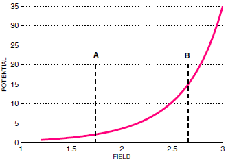
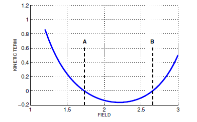
Figure 1: The functions $V_{\rm Ein}(\phi)$ and $K_{\rm Ein}(\phi)$ for some parameters of the action (35), showing a transition from canonical to phantom nature of the scalar field at values marked with the letters A and B.

Let us try to obtain particular solutions of this kind by choosing, as before, a proper shape of the function $r(x)$. This function should possess the following properties:

1. For both wormhole and black universes, a minimum of $r(x)$ must exist (located at $x=0$ without loss of generality), so that

   $$r(0)=a,\qquad r^{\prime}(0)=0,\qquad r^{\prime\prime}(0)>0,\qquad a={\rm const}>0.$$

2. By definition, in a trapped-ghost configuration it must be $h(\phi)<0$ near a minimum of $r$, and $h(\phi)>0$ far from it. By (16c), this implies $r^{\prime\prime}>0$ at small $|x|$ and $r^{\prime\prime}<0$ at sufficiently large $|x|$.

3. For obtaining asymptotically flat or asymptotically (anti-) de Sitter models, we should have

   $$r(x)\approx|x|\qquad{\rm as}\qquad x\to\pm\infty.$$

A simple choice of the function $r(x)$ that satisfies the conditions 1–3 is [30] (see Fig. 2)

$$r(u)=a\frac{(x/a)^{2}+1}{\sqrt{(x/a)^{2}+n}},\hskip 28.45274ptn={\rm const}>2,$$ (37)

where $a$ is is an arbitrary constant, related to the throat radius $r(0)$ by $r(0)=a/\sqrt{n}$, and the value of $a$ can be used as a length scale. Note that the function (37) is different from $r(x)$ used in [24, 29], and the resulting expressions slightly simpler than there.

Further on we put $a=1$; this actually means that the length scale remains arbitrary, but $r$ and $m$ (it is the Schwarzschild mass in our geometrized units) and other quantities with the dimension of length are expressed in units of $a$, accordingly, $B$, $V$ and other quantities with the dimension $\rm(length)^{-2}$ are expressed in units of $a^{-2}$, etc.; the quantities $A,\phi,h$ are dimensionless. Since

$$r^{\prime\prime}(x)=\frac{x^{2}(2-n)+n(2n-1)}{(x^{2}+n)^{5/2}},$$ (38)

we obtain $r^{\prime\prime}>0$ at $x^{2}<n(2n-1)/(n-2)$ and $r^{\prime\prime}<0$ at larger $|x|$, as required; it is also clear that $r\approx|x|$ at large $|x|$. It guarantees $h<0$ at small $|x|$ and $h>0$ at large $|x|$ (see Fig. 2, right panel).

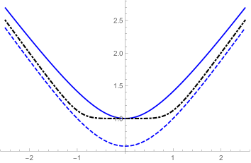
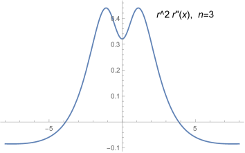
Figure 2: Left: Plots of $r(x)$ under different assumptions: by (29) (solid), by (37), $n=3$ (trapped ghost, dashed), and by (45) (long throat, dot-dashed). Right: Plot of $r^{2}r^{\prime\prime}$ for (37), $n=3$; zeros of this function show the surfaces $h(\phi)=0.$

To avoid cumbersome expressions for $B(x)$ and other quantities, let us restrict our discussion to the value $n=3$. An inspection shows that a particular choice of the parameter $n>2$ does not change the qualitative features of the solutions.

Integrating (28) for $n=3$, we obtain

$$B=B_{0}+\frac{26+24x^{2}+6x^{4}+3mx(69+100x^{2}+39x^{4})}{6(1+x^{2})^{3}}+\frac{39m}{2}\arctan x,$$ (39)

where $B_{0}$ is an integration constant.

Now suppose that our system is asymptotically flat as $x\to+\infty$. Since $B=A/r^{2}$ and $A\to 1$ at infinity, we require $B\to 0$ as $x\to\infty$ and thus fix $B_{0}$ as

$$B_{0}=-\frac{39\pi m}{4}.$$ (40)

The form of $B(x)$ (and accordingly $A(x)=Br^{2}$) substantially depends on the mass $m$, see Fig. 3. It is clear that with $m<0$ we obtain $B(x)$ that tends to a positive constant as $x\to-\infty$, so that $A\sim r^{2}$, and a wormhole with an AdS asymptotic behavior at the far end is obtained (an M-AdS wormhole for short, where M stands for Minkowski). If $m=0$, we obtain a twice asymptotically flat (M-M) wormhole. Lastly, if $m>0$, then $B(x)$ changes its sign at some $x$ and tends to a negative constant, which means that there is a black universe tending to de Sitter geometry as $x\to-\infty$, in full analogy with our first example (29)–(34).

Now the metric is known completely, while $\phi(x)$ and $V(\phi(x))$ are found, as before, from Eqs. (16c) and (16b). To construct $V$ as an unambiguous function of $\phi$ and to find $h(\phi)$, it makes sense to use the parametrization freedom for $\phi(x)$ and to choose

$$\phi(x)=\frac{1}{\sqrt{3}}\arctan\frac{x}{\sqrt{3}},$$ (41)

a behavior common to kink configurations, such that $\phi$ has a finite range: $\phi\in(-\phi_{0},\phi_{0})$, $\phi_{0}=\pi/(2\sqrt{3})$. Thus we have $x=\sqrt{3}\tan(\sqrt{3}\phi)$, ant its substitution to the expression for $V(x)$ found from (16b) gives $V(\phi)$ defined in this finite range.

The kinetic coupling function $h(\phi)$ is then expressed from (16c):

$$h(\phi)=\frac{x^{2}-15}{x^{2}+1}=\frac{3\tan^{2}(\sqrt{3}\phi)-15}{3\tan^{2}(\sqrt{3}\phi)+1}.$$ (42)

This function is also defined on the interval $(-\phi_{0},\phi_{0})$, which may be extended to ${\mathbb{R}}$ if we suppose $h(\phi)\equiv 1$ at $|\phi|\geq\phi_{0}$. As is clear, the NEC is violated where and only where $h(\phi)<0$.

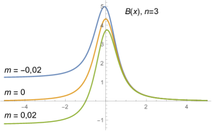
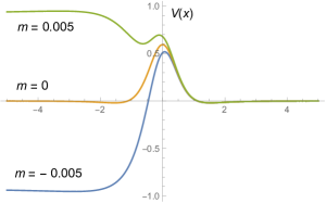
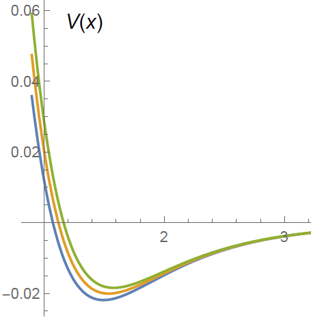
Figure 3: Plots of $B(x)$ (left) and $V(x)$ (middle) for different values of $m$ in a model with $r(x)$ given by Eq. (37) with $n=3$. With $m<0$ we obtain an asymmetric M-AdS wormhole, with $m=0$ a symmetric M-M wormhole, and with $m>0$ a black universe with de Sitter behavior as $x\to-\infty$. The right panel shows the behavior of $V$ at larger $x$, where the curves almost merge. (The colors there have the same meaning as in other panels.)

For $V(x)$ we obtain [30]

$${}V(x)=\frac{1}{12(1+x^{2})^{2}(3+x^{2})^{3}}\Big{\{}32(-6+x^{2}+3x^{4})$$

$${}\hskip 72.26999pt+6mx(2655+6930x^{2}+5420x^{4}+1326x^{6}+117x^{8})$$

$${}\hskip 72.26999pt+117m(1+x^{2})^{2}(15+89x^{2}+29x^{4}+3x^{6})(-\pi+2\arctan x)\Big{\}}.$$ (43)

The function $V(\phi)$ can also be extended to the whole real axis, $\phi\in{\mathbb{R}}$, by putting $V(\phi)\equiv 0$ at all $\phi\geq\phi_{0}$ (since $V(x=+\infty)=0$) and $V(\phi)=V(-\phi_{0})>0$ at all $\phi<-\phi_{0}$.

One can easily verify that the values of $B(x)$ as $x\to-\infty$ are directly related to the asymptotic values of the potential $V$, which plays the role of an effective cosmological constant at large negative $x$:

$$V(-\infty)=117m\pi/2=-3B(-\infty).$$ (44)

We see that the trapped-ghost solution preserves all qualitative features of the simplest solution with the dependence (29) of the spherical radius.

Other, more complicated solutions with diverse global structures are obtained if, besides a scalar field, we introduce an electromagnetic field. Such solutions, including M-M and M-AdS wormholes as well as regular black holes having up to three horizons (up to four horizons if asymptotic flatness is not required), have been found in [30]; their structures turn out to be quite similar to those obtained earlier with a purely phantom scalar field [28].

3.5 Wormholes with an invisible ghost and a long throat

In the previous subsection, having admitted the existence of phantom fields, we discussed a way to explain why they are not observed under usual conditions using the “trapped ghosts” concept. Another way to explain the same is what may be called the “invisible ghost” concept, which means that the phantom field decays rapidly enough at infinity and is there too weak to be observed [52, 56]. To achieve this goal, we need rapidly decaying quantities $\phi^{\prime}$ and hence, by Eq. (16c) $r^{\prime\prime}/r$. Let us therefore replace the previous ansatz (29), $r=(a^{2}+x^{2})^{1/2}$, with [56]

$$r(x)=a(1+x^{2n})^{1/(2n)},\hskip 28.45274ptn\in{\mathbb{N}},$$ (45)

where $a>0$ is, as before, an arbitrary constant, now equal to the throat radius. We will again put $a=1$, so that lengths are expressed in units of the throat radius; the quantities like $B(x)$ and $V(x)$ with the dimension (length)^-2 are expressed in units of $a^{-2}$, while the dimensionless quantities $A(x)$ and $\phi(x)$ are insensitive to this assumption.

The value $n=1$ returns us to the ansatz (29). Higher values of $n$ lead to a new feature of the space-time geometry: the spherical radius $r(x)$ is changing quite slowly near the throat $x=0$, making it possible to call it a long throat, see the dot-dashed curve in Fig. 2, left panel. At large $|x|$ we now have $r^{\prime\prime}/r\approx(2n-1)x^{-2n-2}$, hence $\phi^{\prime}\sim 1/x^{n+1}$, which at large enough $n$ conforms to the “invisible ghost” concept.

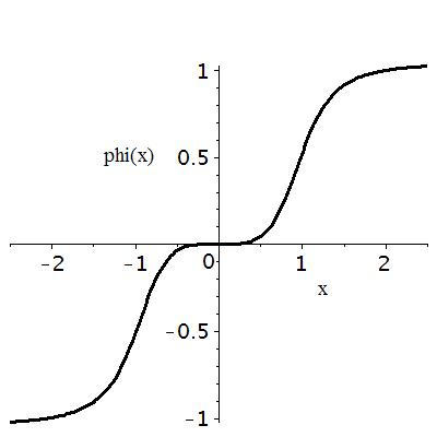
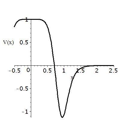
Figure 4: The scalar field $\phi(x)$ (left) and the potential $V(x)$ (right) for $n=4$.

Let us put $m=0$, restricting ourselves to massless wormholes. Then $B^{\prime}(x)$ (28) is an odd function:

$$B^{\prime}(x)=-\frac{2x}{(x^{2n}+1)^{2/n}},$$ (46)

whose integration gives

$$B(x)=-x^{2}F\Big{(}\frac{1}{n},\frac{2}{n};1+\frac{1}{n};-x^{2n}\Big{)}+B_{0},$$ (47)

where $B_{0}$ is an integration constant, and $F(a,b;c,z)$ is the Gaussian hypergeometric function. Assuming asymptotic flatness at large positive $x$, since $B=A/r^{2}$ and $A\to 1$ at infinity, we require $B\to 0$ as $x\to\infty$ and thus fix $B_{0}$ as

$$B_{0}=\lim\limits_{x\to\infty}x^{2}F\Big{(}\frac{1}{n},\frac{2}{n};1+\frac{1}{n};-x^{2n}\Big{)}$$ (48)

We see that it is a twice asymptotically flat (M-M) wormhole, and a plot of $B(x)$ is similar to the curve $m=0$ in Fig. 3 (left). Curiously, the behavior of $A(x)$ shows that there is a domain of repulsive gravity around the throat.

Now the metric is known completely, while $\phi(x)$ and $V(\phi(x))$ are again easily found from Eqs. (16c) and (16b). The expression for the scalar field $\phi(x)$ in the case $n=4$ is (assuming $\phi(0)=0$)

$$\phi(x)=\frac{\sqrt{7}}{4}(\mathop{\rm sign}\nolimits x)\arctan(x^{4}),$$ (49)

see Fig. 4 (left). For the potential $V(x)$ there is rather a cumbersome expression in terms of hypergeometric functions, gamma functions and Legendre functions, and we will not present it here. It is plotted in Fig. 4 (right). Since $V(x)$ is an even function, the plot is restricted to $x\geq 0$.

Models with diverse global structures emerge if there is a nonzero Schwarzschild mass $m$ or/and, besides a scalar field, we consider an electromagnetic field with the corresponding electric or magnetic charge. Examples of such solutions, including M-M, M-dS (de-Sitter), M-AdS (anti de-Sitter) wormholes and regular black holes containing up to four horizons, can be found in [28, 29, 30, 52]. The global qualitative features of our present field system are similar to those described above, and the same kinds of regular solutions can be obtained using the same methods.

4 The stability problem

4.1 Spherically symmetric perturbation equations

The stability problem is of great importance while studying any equilibrium configurations since only stable or very slowly decaying ones have a chance to exist for a sufficiently long time. On the other hand, the development of instabilities can lead to a lot of important phenomena, such as, for example, structure formation in the early Universe and Supernova explosions.

Let us discuss the stability problem for configurations with scalar fields like those described in the previous section. The problem is whether an initial small time-dependent perturbation can grow strongly enough to destroy the system. As in a majority of such studies, we consider linear perturbations and neglect their quadratic and higher-order combinations. Moreover, we restrict the study to perturbations that preserve spherical symmetry (in other words, only radial, or monopole perturbations). On one hand, they are the simplest, but on the other, they are the most “dangerous” ones since they lead to instabilities in many known models with self-gravitating scalar fields [31, 32, 33, 34, 35, 36, 37, 38]. Other modes of perturbations are usually found to be stable, see, e.g., [38, 57]. Let us suppose that some static solution is already known (the solutions described above being special cases) and consider its time-dependent perturbations.

We will follow the lines of [3, 37, 52, 58] and consider the same field system as before, that is, (12), (13), (14), with the scalar field SET:

$$T_{\mu}^{\nu}[\phi]=h(\phi)[2\phi_{\mu}\phi^{\nu}-\delta_{\mu}^{\nu}\phi^{\alpha}\phi_{\alpha}]+\delta_{\mu}^{\nu}V(\phi),$$ (50)

The general spherically symmetric metric can be written in the form (2), that is,

$$ds^{2}={\,\rm e}^{2\gamma}dt^{2}-{\,\rm e}^{2\alpha}du^{2}-{\,\rm e}^{2\beta}d\Omega^{2},$$ (51)

where now $\gamma$, $\alpha$ and $\beta$ are functions of both the radial coordinate $u$ and time $t$. We use again the notation $r(u)\equiv{\,\rm e}^{\beta}$ and preserve the freedom of choosing the coordinate $u$.

Consider linear spherically symmetric perturbations of static solutions (known by assumption) to the field equations due to (12). Now we write

$$\phi(u,t)=\phi(u)+\delta\phi(u,t),\qquad\gamma(u,t)=\gamma(u)+\delta\gamma$$ (52)

for the scalar field and the metric function $gamma$ and similarly for all other quantities, assuming small “deltas”.

All nonzero components of the Ricci tensor are (with only linear terms with respect to time derivatives)

$$R^{t}_{t} = {\,\rm e}^{-2\gamma}(\ddot{\alpha}+2\ddot{\beta})-{\,\rm e}^{-2\alpha}[\gamma^{\prime\prime}+\gamma^{\prime}(\gamma^{\prime}-\alpha^{\prime}+2\beta^{\prime})],$$ (53)

$${}R^{u}_{u} = {\,\rm e}^{-2\gamma}\ddot{\alpha}-{\,\rm e}^{-2\alpha}[\gamma^{\prime\prime}+2\beta^{\prime\prime}+\gamma^{\prime}{}^{2}+2\beta^{\prime}{}^{2}-\alpha^{\prime}(\gamma^{\prime}+2\beta^{\prime})],$$ (54)

$${}R^{\theta}_{\theta} = R^{3}_{3}={\,\rm e}^{-2\beta}+{\,\rm e}^{-2\gamma}\ddot{\beta}-{\,\rm e}^{-2\alpha}[\beta^{\prime\prime}+\beta^{\prime}(\gamma^{\prime}-\alpha^{\prime}+2\beta^{\prime})],$$ (55)

$${}R_{tu} = 2[\dot{\beta}^{\prime}+\dot{\beta}\beta^{\prime}-\dot{\alpha}\beta^{\prime}-\dot{\beta}\gamma^{\prime}],$$ (56)

where dots and primes denote $\partial/\partial t$ and $\partial/\partial u$, respectively.

The background (zero-order, static) scalar field equation and the ${t\choose t}$, ${u\choose u}$, and ${\theta\choose\theta}$ components of the Einstein equations (4) read

$$2h[\phi^{\prime\prime}+\phi^{\prime}(\gamma^{\prime}+2\beta^{\prime}-\alpha^{\prime})]+h^{\prime}\phi^{\prime} = {\,\rm e}^{2\alpha}dV/d\phi;$$ (57)

$${}\gamma^{\prime\prime}+\gamma^{\prime}(\gamma^{\prime}+2\beta^{\prime}-\alpha^{\prime}) = -{\,\rm e}^{2\alpha}V;$$ (58)

$${}\gamma^{\prime\prime}+2\beta^{\prime\prime}+\gamma^{\prime}{}^{2}+2\beta^{\prime}{}^{2}-\alpha^{\prime}(\gamma^{\prime}+2\beta^{\prime}) = -2h\phi^{\prime 2}-{\,\rm e}^{2\alpha}V;$$ (59)

$${}-{\,\rm e}^{2\alpha-2\beta}+\beta^{\prime\prime}+\beta^{\prime}(\gamma^{\prime}+2\beta^{\prime}-\alpha^{\prime}) = -V{\,\rm e}^{2\alpha}.$$ (60)

The first-order perturbed equations (scalar, $R_{ut}=\ldots$, and $R^{\theta}_{\theta}=\ldots$) have the form

$${}2{\,\rm e}^{2\alpha-2\gamma}h\delta\ddot{\phi}-2h[\delta\phi^{\prime\prime}+\delta\phi^{\prime}(\gamma^{\prime}+2\beta^{\prime}-\alpha^{\prime})+\phi^{\prime}(\delta\gamma^{\prime}+2\delta\beta^{\prime}-\delta\alpha^{\prime})]$$

$${}\hskip 72.26999pt-2\delta h[\phi^{\prime\prime}+\phi^{\prime}(2\beta^{\prime}+\gamma^{\prime}-\alpha^{\prime})]-h^{\prime}\delta\phi^{\prime}-\phi^{\prime}\delta h^{\prime}+\delta({\,\rm e}^{2\alpha}V_{\phi})=0,$$ (61)

$${}\delta\dot{\beta}^{\prime}+\beta^{\prime}\delta\dot{\beta}-\beta^{\prime}\delta\dot{\alpha}-\gamma^{\prime}\delta\dot{\beta}=-h\phi^{\prime}\delta\dot{\phi},$$ (62)

$${}\delta({\,\rm e}^{2\alpha-2\beta})+{\,\rm e}^{2\alpha-2\gamma}\delta\ddot{\beta}-\delta\beta^{\prime\prime}-\delta\beta^{\prime}(\gamma^{\prime}+2\beta^{\prime}-\alpha^{\prime})$$

$${}\hskip 72.26999pt\hskip 28.45274pt-\beta^{\prime}(\delta\gamma^{\prime}+2\delta\beta^{\prime}-\delta\alpha^{\prime})=\delta({\,\rm e}^{2\alpha}V).$$ (63)

Equation (62) is easily integrated in $t$; being interested in time-dependent perturbations only, we omit the arbitrary function of $u$ that emerges at this integration and describes static perturbations. This leads to

$$\delta\beta^{\prime}+\delta\beta(\beta^{\prime}-\gamma^{\prime})-\beta^{\prime}\delta\alpha=-h\phi^{\prime}\delta\phi.$$ (64)

Our system possesses two independent forms of arbitrariness: the freedom to choose a radial coordinate $u$ in the static background solution, and the perturbation gauge, a freedom related to the choice of a reference frame in perturbed space-time. As a result, we can impose some relation containing $\delta\alpha,\ \delta\beta$, etc. Further on we employ both kinds of freedom. All the above equations are written in a universal form, where neither the $u$ coordinate nor the perturbation gauge are fixed.

Let us simplify the equations by choosing the “tortoise” coordinate $u=z$, specified by the condition $\alpha=\gamma$ (it is the best for wave equations), and the perturbation gauge $\delta\beta\equiv 0$. Then from Eq. (64) we find $\delta\alpha$ in terms of $\delta\phi$ (now the prime stands for $d/dz$):

$$\beta^{\prime}\delta\alpha=h(\phi)\phi^{\prime}\delta\phi.$$ (65)

From Eq. (4.1) we find $\delta\gamma^{\prime}-\delta\alpha^{\prime}$ in terms of $\delta\alpha$ and $\delta\phi$:

$$\beta^{\prime}(\delta\gamma^{\prime}-\delta\alpha^{\prime})=2{\,\rm e}^{2\alpha-2\beta}\delta\alpha-\delta({\,\rm e}^{2\alpha}V).$$ (66)

With all that substituted to (4.1), the following wave equation is obtained:

$${}\delta\ddot{\phi}-\delta\phi^{\prime\prime}-\delta\phi^{\prime}(2\beta^{\prime}+h^{\prime}/h)+U\delta\phi=0,$$ (67)

$${}U\equiv{\,\rm e}^{2\alpha}\biggl{[}\frac{2h\phi^{\prime 2}}{\beta^{\prime 2}}(V-{\,\rm e}^{-2\beta})+\frac{2\phi^{\prime}}{\beta^{\prime}}V_{\phi}+\frac{V_{\phi\phi}}{2h}\biggr{]}-\frac{h^{\prime\prime}+h_{\phi}\phi^{\prime\prime}}{2h}-\frac{2\beta^{\prime}h^{\prime}}{h},\hskip 28.45274pt$$ (68)

where the index $\phi$ denotes $d/d\phi$. The expression (68) for $U$ is a generalization of the one obtained in [37] for scalar-vacuum systems with $h=\epsilon=\pm 1$.

Next, the first-order derivative of $\delta\phi$ in (67) is removed by the substitution

$$\delta\phi=\psi(z,t){\,\rm e}^{-\eta},\hskip 28.45274pt\eta^{\prime}=\beta^{\prime}+\frac{h^{\prime}}{2h},$$ (69)

which reduces the wave equation to the canonical form

$$\ddot{\psi}-\psi^{\prime\prime}+V_{\rm eff}(z)\psi=0,$$ (70)

with the effective potential

$${}V_{\rm eff}(z)=U+\eta^{\prime\prime}+\eta^{\prime}{}^{2}={\,\rm e}^{2\alpha}\biggl{[}\frac{2h\phi^{\prime 2}}{\beta^{\prime 2}}(V-{\,\rm e}^{-2\beta})+\frac{2\phi^{\prime}}{\beta^{\prime}}V_{\phi}-\frac{h_{\phi}}{4h^{2}}V_{\phi}+\frac{V_{\phi\phi}}{2h}\biggr{]}+\beta^{\prime\prime}+\beta^{\prime 2}.\qquad$$ (71)

One more substitution, using the static nature of the background,

$$\psi(x,t)=Y(x){\,\rm e}^{i\omega t},\hskip 28.45274pt\omega={\rm const},$$ (72)

leads to the Schrödinger-like equation

$$Y^{\prime\prime}+[\omega^{2}-V_{\rm eff}(x)]Y=0.$$ (73)

Now, if there exists a nontrivial solution to (73) such that $\mathop{\rm Im}\nolimits\omega<0$, for which some physically reasonable conditions hold at the ends of the range of $z$ (including the absence of ingoing waves), then we can conclude that the static background system is unstable since the perturbation $\delta\phi$ can exponentially grow with time. Otherwise our static system is stable in the linear approximation. The value $\omega=0$ makes possible a linear growth of perturbations. As usual in such studies, the stability problem is thus reduced to a boundary-value problem for Eq. (73) — see, e.g., [3, 37, 38, 31, 59, 32, 33, 35, 57].

The gauge $\delta\beta=0$ is convenient for calculations but looks doubtful when applied to configurations with throats. The reason is that writing $\delta\beta=0$, we suppose that the throat radius is not subject to perturbations, whereas its changes are in general admissible [59, 35, 3]. It might seem that the pole in $V_{\rm eff}$ related to $\delta\beta$ in the denominator in (68) is an artifact of this gauge. It turns out, however, in full similarity with [35, 37, 3], that Eq. (73) is in fact gauge-invariant, and the perturbation $\delta\phi$ represents a certain gauge-invariant quantity in the gauge $\delta\beta=0$. This issue is discussed in detail, e.g., in [37, 3, 58].

4.2 Perturbations near a generic throat

Since Eq. (73) is gauge-invariant, boundary value problems in the stability study are really meaningful. However, the problems are rather complicated due to the singular nature of the effective potential $V_{\rm eff}$. The singularities are of two kinds: one is related to throats, if any, due to terms containing $1/\beta^{\prime 2}$ and $1/\beta^{\prime}$ in $V_{\rm eff}$ (since $\beta^{\prime}=0$ on a throat); the other takes place at transition surfaces from usual to phantom scalar fields because $V_{\rm eff}$ contains terms proportional to $h^{-2}$ and $h^{-1}$, while $h=0$ at such a transition. Let us first discuss the singularities related to throats, following [58] and partly [35, 37].

Suppose that there is a throat at (say) $z=0$, where the spherical radius $r(z)={\,\rm e}^{\beta}$ possesses a generic minimum, such that $r(z)=r_{0}+{{\textstyle\frac{1}{2}}}r_{2}z^{2}+o(z^{2})$, where $r_{0}>0,\ r_{2}>0$. Also, without loss of generality, close to the throat we put $h(\phi)=-1$ since due to (16c) it should be $h<0$, and $h(\phi)=-1$ is obtained by a regular redefinition of $\phi$. Then, from the zero-order (background) equations it follows that near the throat

$$V_{\rm eff}(\phi)=2/z^{2}+O(1),$$ (74)

and a contribution of the form $O(z^{-1})$ is absent. Thus we have an infinite potential wall that separates perturbations to the left ($z<0$) of the throat from those to the right ($z>0$) because a natural boundary condition at $z=0$ is $\psi(0)=0$. All other perturbations also vanish at $z=0$. As a result, a mode of evident physical significance, connected with time-dependent perturbations of the throat radius, drops off from the consideration.

A way to solve this problem is to apply a Darboux transformation (see, e.g., [60] for a recent presentation and application to BH physics), also called S-deformation, to the effective potential $V_{\rm eff}$. It was used in [61, 62] in order to convert a partly negative potential to a positive-definite one in a stability problem for higher-dimensional black holes. Later on this method was used by Gonzalez et al. [35] for transforming a singular effective potential for perturbations of anti-Fisher wormholes to a nonsingular one, which has led to finding an exponentially growing mode. Thus such wormholes are unstable, the instability being connected with a changing radius of the throat. The same method in a slightly more general formulation was applied in [37, 38] in a stability study for other spherically symmetric configurations with throats, in particular, some black universe models. The method can be briefly described as follows.

Consider a wave equation of the type (70)

$$\ddot{\psi}-\psi^{\prime\prime}+W(z)\psi=0,$$ (75)

with an arbitrary potential $W(z)$ (the above potential $V_{\rm eff}$ is its specific example). The potential $W(z)$ may be presented in the form

$$W(z)=S^{2}(z)+S^{\prime},$$ (76)

which may be treated as a Riccati equation with respect to $S(z)$, and its solution makes it possible to find $S(z)$ for given $W(z)$. Then we can rewrite Eq. (75) as

$$\ddot{\psi}+(\partial_{z}+S)(-\partial_{z}+S)\psi=0.$$ (77)

If we introduce the new function

$$\chi=(-\partial_{z}+S)\psi,$$ (78)

then, applying the operator $-\partial_{z}+S$ to the left-hand side of Eq. (77), we obtain a wave equation for $\chi$:

$$\ddot{\chi}-\chi^{\prime\prime}+W_{1}(z)\chi=0,$$ (79)

with the new effective potential

$$W_{1}(x)=-S^{\prime}+S^{2}=-W(z)+2S^{2}.$$ (80)

If a static solution $\psi_{s}(z)$ of Eq. (75) is known, so that $\psi^{\prime\prime}_{s}=W(z)\psi_{s}$, then we can choose

$$S(z)=\psi^{\prime}_{s}/\psi_{s}$$ (81)

to use in the above transformation. Next, if we assume that $W(x)\approx az^{-n}$ at small $z$ and require that $W_{1}$ should be finite at $z=0$, then, using (80), we find that a necessary condition for removing such a singularity is $n=1,\ a=2$, that is, $W\approx 2/z^{2}$. Fortunately, according to Eq. (74), the potential $V_{\rm eff}$ exhibits precisely the required behavior. One can notice that this regularization works for a positive pole, $W\to+\infty$ as $z\to 0$, and removes a potential wall in $W(z)$ whereas a potential well cannot be removed in this way. A point of interest is that the Darboux transformation, being isospectral when it connects regular wave equations, loses isospectrality in the singular case and actually reveals a mode of perturbations which was hidden when the wave equation had a singular potential.

From (80) with finite $W_{1}$ it also follows that at small $z$

$$S\approx-1/z\ \ \ \Rightarrow\ \ \ \psi_{s}\propto 1/z.$$ (82)

Summarizing, we see that the singularity of the effective potential $V_{\rm eff}$ occurring at a throat can be regularized for a throat of generic shape [35, 37]. What is also of great importance is that solutions to the regularized wave equation lead to regular perturbations of the scalar field and the metric. It was this procedure that has led to a proof of the instability of anti-Fisher (Ellis type [9, 10]) wormholes [35] and other configurations with scalar fields in GR [37, 38]. Examples of such results are depicted in Fig. 5:

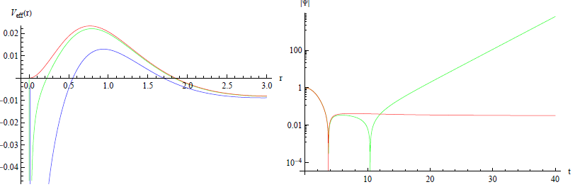
Figure 5: Regularized effective potentials for perturbations of some black-universe solutions (29), (30) (left) and the time-domain profiles of their time evolution [38] (right). Only one of the models under study is stable (the time-domain plot is asymptotically constant), it is the model where the throat coincides with the event horizon.

4.3 Perturbations near the surface $h=0$

The effective potential $V_{\rm eff}$ also possesses another kind of singularities at values of the radial coordinate where the factor $h(\phi)$ in (12) changes its sign, if certainly such values of $\phi$ do exist, which happens in the trapped ghost situation. The nature of these singularities is different from that described above. Somewhat similar singularities were previously found in systems with conformal continuations at the corresponding transition surfaces [16, 32, 33]. The latter phenomenon takes place, for example, in scalar-tensor theories of gravity where it can happen that at certain values of the parameters the whole Einstein-frame manifold maps to only a region in the Jordan-frame manifold (or vice versa). It was found that for static, spherically symmetric configurations of this kind, monopole perturbations obey wave equations of the form (70) with effective potentials possessing singularities of the form

$$V_{\rm eff}\approx-1/(4z^{2})\quad\ {\rm as}\quad z\to 0$$ (83)

where $z=0$ is a transition surface on which the Einstein frame terminates while the Jordan frame has a regular metric [32].

Returning to our system, let us assume that close to the value of $z$ at which $h=0$ (let it be $z=0$) the metric functions $\alpha=\gamma$ (according to our “tortoise” gauge) and $\beta$ as well as the scalar $\phi$ are regular and can be approximated by the Taylor expansions

$${}\alpha=\alpha_{0}+\alpha_{1}z+\ldots,\quad\ \beta=\beta_{0}+\beta_{1}z+\ldots,\quad\ \phi=\phi_{0}+\phi_{1}z+{{\textstyle\frac{1}{2}}}\phi_{2}+\ldots,$$

$${}h(z)=h_{1}z+{{\textstyle\frac{1}{2}}}h_{2}z^{2}+\ldots,\qquad\phi_{1}\neq 0,\ \ \ h_{1}\neq 0.$$ (84)

One can show that in such a generic situation the potential (71) is approximated near $z=0$ by the Laurent series

$$V_{\rm eff}(z)=-\frac{1}{4z^{2}}+\frac{1}{z}\biggl{[}\frac{h_{2}}{h_{1}}+2\Big{(}\beta_{1}-\alpha_{1}+\frac{\phi_{2}}{\phi_{1}}\Big{)}\biggr{]}+O(1).$$ (85)

Thus the surface where $h=0$ is a location of a potential well of infinite depth. In quantum mechanics such a well, according to the stationary Schrödinger equation, would cause the existence of arbitrarily deep negative energy levels. As regards the stability study, it would be tempting to conclude, by analogy, that there are perturbation modes with $\omega^{2}<0$ and arbitrarily large $|\omega|$, and then the corresponding perturbations would grow as ($\delta\phi\sim e^{|\omega|t}$), immediately leading the system out of a linear regime and making necessary a nonlinear or nonperturbative analysis.

However, in the stability study, the quantities $\psi$ in Eq. (70) or $Y$ in (73) are subject to quite different physical requirements: the perturbation $\delta\phi$ should remain finite in the whole space and also vanish at infinities or horizons, while in quantum mechanics the only requirement is quadratic integrability of $\psi$.

With the potential (85), the general solution of (73) at small $z$ has, independently of $\omega$, the leading terms

$$Y(z)=\sqrt{|z|}(C_{1}+C_{2}\ln|z|)+O(z^{3/2}),\qquad C_{1},\ C_{2}={\rm const}.$$ (86)

Furthermore, according to (69), $\delta\phi\sim Y/\sqrt{h}\sim Y/\sqrt{|x|}$, and

$$\delta\phi\sim C_{1}+C_{2}\ln|z|+O(z),$$ (87)

so physically meaningful perturbations correspond to $C_{2}=0$. The negative pole of (85) thus leads to a new constraint that should be considered together with the ordinary boundary conditions specifying the boundary-value problem for the Schrödinger equation. From this additional constraint it may follow that this boundary-value problem does not possess any discrete spectrum. Indeed, assuming a background configuration with a surface where $h=0$ (say, at $z=0$), Eq. (73) has a solution satisfying the boundary conditions imposed at infinities and/or a horizon; then there will be in general a zero probability that such a solution is finite at $z=0$. A possible exception is a ${\mathbb{Z}}_{2}$-symmetric background with respect to the surface $z=0$ (then the whole boundary-value problem is the same for $z<0$ and $z>0$, and the whole spectrum is also the same), but in our system it is manifestly not such a case since we have $h>0$ on one side of the surface $z=0$ and $h<0$ on the other. A situation like this was discussed in [63, 64] for the stability of BHs with a conformal scalar field [65, 66], and after all, using some more reasoning, it was concluded that these black holes are stable under monopole perturbations [64].

(Unlike this situation, in a quantum-mechanical problem setting, the quadratic integrability requirement for $Y(z)$ is satisfied as long as $\int z^{n}\ln^{2}z\,dz<\infty$ near $z=0$ for any $n\geq 0$. A quantum particle in such a potential well, as is sometimes said, “falls onto the center” [67] since, as one descends to deeper and deeper negative energy levels, the wave function becomes more and more concentrated near $z=0$.)

We can conclude that if there is a transition surface from canonical to phantom scalar field, it plays a strong stabilizing role for any such configuration. However, it looks impossible to say about a particular trapped-ghost solution, whether it is stable or not: an individual investigation is necessary since a conclusion must depend on the details of each model.

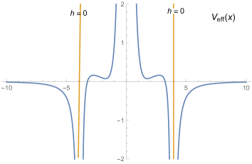
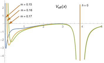
Figure 6: Effective potentials $V_{\rm eff}=V_{\rm eff}(x)$ for perturbations of trapped-ghost solutions with the metric coefficients (37) and (39), $n=3$. Left: $V_{\rm eff}$ for a massless ($m=0$) symmetric wormhole. Right: $V_{\rm eff}$ for trapped-ghost black universe solutions with $m>0$, in which the minimum of $r$ ($x=0$) is beyond the horizon. Note that in terms of $z$, the first plot would remain qualitatively the same, whereas in the second one a finite $x>0$ at the horizon would turn into $z=-\infty$.

Figure 6 shows the effective potentials $V_{\rm eff}$ for different trapped-ghost configurations. In the case of a symmetric, twice asymptotically flat wormhole there are four regions separated by poles of $V_{\rm eff}$. The positive pole at $x=0$ can be regularized by an S-transformation as described above, while the poles where $h=0$ impose conditions similar to $C_{2}=0$ in Eq. (87). Thus, for Eq. (73), as many as three boundary-value problems should be considered in three ranges of $z$ separated from each other by $h=0$ points. Though, in this particular solution two of them coincide due to symmetry ($x\leftrightarrow-x$) of the wormhole.

For black-universe solutions without throats outside the horizon, an additional regularization is unnecessary, two boundary-value problems on different sides of the pole at $h=0$ may be solved directly, and the resulting spectra should be then compared to find out whether there are coinciding eigenvalues leading to unstable perturbation modes. A tentative conclusion is that at least for some values of $m$ there is such an unstable mode with $\omega=0$, which means that there are perturbations growing with time by a linear law.

4.4 Perturbations near a long throat

Now, let us apply the above formalism to static solutions where the spherical radius $r(x)$ behaves near the throat like the function (45). More specifically, let the throat be located at $z=0$ and, as $z\to 0$, let the radius $r$ behave as $r\approx r_{0}+O(z^{2n})$ (as is the case with (45)). Then at small $z$, as can be directly verified [56],

$$V_{\rm eff}(z)=2\biggl{[}\Big{(}\frac{\beta^{\prime\prime}}{\beta^{\prime}}\Big{)}^{2}-\frac{\beta^{\prime\prime\prime}}{\beta^{\prime}}\biggr{]}+O(1)=\frac{2(2n{-}1)}{z^{2}}+O(1),$$ (88)

Models with ordinary (generic) throats correspond to $n=1$ and those with long throats to $n>1$.

As described above, for $n=1$ the potential $V_{\rm eff}$ can be regularized using a Darboux transformation, which is a special kind of substitution in Eq. (73): the transformed equation is regular at $z=0$, and solutions to the corresponding boundary-value problem describe regular perturbations of the scalar field and the metric, including those in which the throat radius changes with time. However, a necessary condition for singularity removal is that $V_{\rm eff}=2/z^{2}+O(1)$, which does not hold for $n>1$.

Now suppose that (without loss of generality) at $z=0$ the potential behaves as

$$W(z)=\frac{N}{z^{2}}+O(1),\hskip 28.45274ptN={\rm const},$$ (89)

and apply the S-transformation according to Eqs. (75)–(80). It is then easy to verify that

$$W_{1}(z)=\frac{N_{1}}{z^{2}}+O(1),\hskip 20.00003ptN_{1}=N+1\pm\sqrt{1+4N}.$$ (90)

The minus sign should be chosen here if we wish to “weaken” the pole of $W$, that is, make $N_{1}<N$. In particular, if $N=N_{k}=k(k+1)$, $k\in{\mathbb{N}}$, then the S-transformation leads to a new potential with $N_{k-1}=(k-1)k$, or symbolically

$$N_{k}=k(k+1)\ \ \mathop{\longrightarrow}\limits_{S}\ \ N_{k-1}=(k-1)k.$$ (91)

Therefore, if a potential behaves as $W(z)=-k(k+1)/z^{2}+O(1)$, $k\in{\mathbb{N}}$, then each described step “lowers the order” $k$ by a unit, and after $k$ such steps we obtain a regular potential.

For long throats with radii of the form $r\approx r_{0}+{\rm const}\cdot z^{2n}$, the effective potential (88) thus admits regularization in $k$ steps if $2n=2n_{k}=1+k(k+1)/2$. Thus, for $k=1,2,3,4,5$, the corresponding values of $n=n_{k}$ admitting this procedure are $n=1,2,7/2,11/2,8$, etc. If the quantity $n$ in Eq. (88) does not belong to this sequence, the potential $V_{\rm eff}$ cannot be regularized by S-transformations.

Thus a general formalism for studying the stability of wormhole models with long throats is ready, at least for $n$ belonging to the sequence $n_{k}=1/2+k(k+1)/4$. However, a practical implementation of this formalism for particular models is difficult and requires significant numerical work (now in progress) since even if static background solutions are known analytically, the perturbation equations can be solved only numerically.

We have considered [56], as a tentative study, the stability properties of a configuration with a constant spherical radius $r(x)$, which may be called a maximally long throat. It is not a wormhole since there are no spatial asymptotics. The corresponding static solution to the field equations reduces to the well-known Nariai metric [68] with a constant scalar field, and it has been explicitly shown that it is unstable under linear perturbations. Therefore, one can speculate that a slowly varying radius near a throat does not stabilize a wormhole supported by a phantom scalar field.

5 Conclusion

Having recalled some general properties of static, spherically symmetric space-times in GR, in particular, those with a scalar field source, we have discussed some examples of globally regular solutions, among which are wormholes and black universes. The latter seem to be a viable possible description of a pre-inflationary epoch in cosmology and an attractive opportunity that the cosmic evolution began from a horizon instead of a singularity.

Some of the existing solutions confirm that scalar fields may change their nature from a canonical one to a ghost one in a smooth way without leading to space-time singularities [25, 24, 29, 30]. This circumstance widens the possible choice of scalar field dynamics and, in addition, the possible formulations of scalar-tensor theories of gravity, even though we have so far considered minimally coupled fields only.

More specifically, the trapped ghost concept makes it possible to obtain spherically symmetric wormhole and regular BH models with a ghost behavior in a restricted strong-field region whereas outside it, where any observers can live, the scalar has usual properties. One can speculate that if such ghosts do exist in Nature, they are all confined to strong-field regions (“all genies are sitting in bottles”).

In addition to particular examples of exact solutions, some general properties of static, spherically symmetric scalar field configurations have been revealed:

(i)

Trapped-ghost solutions to the field equations are only possible with nonzero potentials $V(\phi)$.

(ii)

If the Einstein-scalar equations have a twice asymptotically flat solution (be it of trapped-ghost nature or not), then the Schwarzschild mass has different signs at the two infinities, while mirror (${\mathbb{Z}}_{2}$) symmetry with respect to a certain surface is only possible if $m=0$.

(iii)

Transition surfaces between regions of canonical and phantom behavior of a scalar field create a potential well for spherically symmetric perturbations, with a universal shape (see Eq. (85)) for all such models. The finiteness requirement for perturbations on this surface forms an additional constraint that, being added to the standard boundary conditions, restricts the set of possible solutions and thus plays a stabilizing role.

This latter result may seem somewhat unexpected but, in my view, it can raise an interest in trapped-ghost models. One can try to use this opportunity for solving various problems of gravitational physics and cosmology.

Of certain interest are the properties of perturbations near a long throat which is obtained in some of the solutions. More generally, one can conclude that a general formalism for stability studies in the presence of throats and transition surfaces has been prepared, but studies of particular models lead to rather involved numerical tasks to be considered in the near future. Another task is to try to extend the present results to some alternative theories of gravity, such as scalar-tensor and $f(R)$ theories.

One should also mention such a task of utmost importance in the present and future studies as the analysis of observational properties of wormholes, such as gravitational lensing and shadows (see [69, 70, 71] and references therein) as well as possible constraints on their existence that follow from any already known observational data ([72] and references therein).

Acknowledgments

I thank the colleagues from Yerevan University for wonderful hospitality during the conference. I am grateful to Milena Skvortsova, Sergei Bolokhov and Artyom Yurov for helpful discussions. The work was partly performed within the framework of the Center FRPP supported by MEPhI Academic Excellence Project (contract No. 02.a03.21.0005, 27.08.2013). This publication was also supported by the RUDN University program 5-100 and by RFBR grant 16-02-00602.

References

- [1] M. Visser, Lorentzian Wormholes: From Einstein to Hawking (American Institute of Physics, New York, 1995)
- [2] F.S.N. Lobo, Exotic solutions in General Relativity: Traversable wormholes and “warp drive” spacetimes. In: Classical and Quantum Gravity Research, p. 1-78 (Nova Sci. Pub., 2008); ArXiv: 0710.4474.
- [3] K. A. Bronnikov and S. G. Rubin, Black Holes, Cosmology, and Extra Dimensions (World Scientific, 2012).
- [4] K.A. Bronnikov, K.A. Baleevskikh and M.V. Skvortsova, Wormholes with fluid sources: A no-go theorem and new examples. Phys. Rev. D 96, 124039 (2017); arXiv: 1708.08125.02324.
- [5] F.S.N. Lobo (Ed.), Wormholes, Warp Drives and Energy Conditions (Springer, 2017).
- [6] L. Flamm, Beiträge zur Einsteinschen Gravitationstheorie. Phys. Z. 17, 48 (1916).
- [7] M.S. Morris and K.S. Thorne, Wormholes in spacetime and their use for interstellar travel: A tool for teaching general relativity. Am. J. Phys. 56, 395 (1988).
- [8] D. Hochberg and M. Visser, Geometric structure of the generic static traversable wormhole throat. Phys. Rev. D 56, 4745 (1997); gr-qc/9704082.
- [9] K.A. Bronnikov, Scalar-tensor theory and scalar charge. Acta Phys. Pol. B 4, 251 (1973).
- [10] H. Ellis, Ether flow through a drainhole — a particle model in general relativity. J. Math. Phys. 14, 104 (1973).
- [11] K.A. Bronnikov, Spherically symmetric false vacuum: no-go theorems and global structure. Phys. Rev. D 64, 064013 (2001); gr-qc/0104092.
- [12] S.V. Sushkov and Y.-Z. Zhang, Scalar wormholes in cosmological setting and their instability. Phys. Rev. D 77, 024042 (2008); arXiv: 0712.1727.
- [13] K.A. Bronnikov and A.A. Starobinsky, No realistic wormholes from ghost-free scalar-tensor phantom dark energy. JETP Lett. 85, 1 (2007); gr-qc/0612032.
- [14] K.A. Bronnikov and A.A. Starobinsky, Once again on thin-shell wormholes in scalar-tensor gravity. Mod. Phys. Lett. A 24, 1559 (2009); arXiv: 0903.5173.
- [15] K.A. Bronnikov, M.V. Skvortsova and A.A. Starobinsky, Notes on wormhole existence in scalar-tensor and F(R) gravity. Grav. Cosmol. 16, 216 (2010), arXiv: 1005.3262.
- [16] K.A. Bronnikov, Scalar-tensor gravity and conformal continuations, J. Math. Phys. 43, 6096–6115 (2002); gr-qc/0204001.
- [17] K.A. Bronnikov and A.M. Galiakhmetov, Wormholes without exotic matter in Einstein-Cartan theory. Grav. Cosmol. 21, 283 (2015); arXiv: 1508.01114.
- [18] K.A. Bronnikov and A.M. Galiakhmetov, Wormholes and black universes without phantom fields in Einstein-Cartan theory. Phys. Rev. D 94, 124006 (2016); arXiv: 1607.07791.
- [19] Gustavo Dotti, Julio Oliva, and Ricardo Troncoso, Static wormhole solution for higher-dimensional gravity in vacuum. Phys. Rev. D 75, 024002 (2007); hep-th/0607062.
- [20] Tiberiu Harko, Francisco S.N. Lobo, M.K. Mak, and Sergey V. Sushkov, Gravitationally modified wormholes without exotic matter, arXiv: 1301.6878.
- [21] K.A. Bronnikov and S.-W. Kim, Possible wormholes in a brane world. Phys. Rev. D 67, 064027 (2003), gr-qc/0212112.
- [22] R.V. Korolev and Sergey V. Sushkov, Exact wormhole solutions with nonminimal kinetic coupling, arXiv: 1408.1235.
- [23] Sayan Kar, Sayantani Lahiri, and Soumitra SenGupta, Can extra dimensional effects allow wormholes without exotic matter? Phys. Lett. B 750, 319 (2015); arXiv: 1505.06831.
- [24] K.A. Bronnikov and S.V. Sushkov, Trapped ghosts: a new class of wormholes. Class. Quantum Grav. 27, 095022 (2010); arXiv: 1001.3511.
- [25] H. Kroger, G. Melkonian and S.G. Rubin, Cosmological dynamics of scalar field with non-minimal kinetic term. Gen. Rel. Grav. 36, 1649 (2004); astro-ph/0310182.
- [26] K.A. Bronnikov and J.C. Fabris, Regular phantom black holes. Phys. Rev. Lett. 96, 251101 (2006).
- [27] K.A. Bronnikov, V.N. Melnikov and H. Dehnen, Regular black holes and black universes. Gen. Rel. Grav. 39, 973 (2007).
- [28] S.V. Bolokhov, K.A. Bronnikov, and M.V. Skvortsova, Magnetic black universes and wormholes with a phantom scalar. Class. Quantum Grav.29, 245006 (2012).
- [29] K.A. Bronnikov and E.V. Donskoy, Black universes with trapped ghosts. Grav. Cosmol. 17, 176–180 (2011).
- [30] K.A. Bronnikov, E.V. Donskoy, and P. Korolyov, Magnetic wormholes and black universes with trapped ghosts. Vestnik RUDN No. 2, 139–149 (2013).
- [31] K.A. Bronnikov, A.V. Khodunov. Scalar field and gravitational instability. Gen. Rel. Grav.11, 13 (1979).
- [32] K.A. Bronnikov and S.V. Grinyok, Instability of wormholes with a nonminimally coupled scalar field, Grav. Cosmol. 7, 297 (2001); gr-qc/0201083.
- [33] K.A. Bronnikov and S.V. Grinyok, Conformal continuations and wormhole instability in scalar-tensor gravity. Grav. Cosmol. 10, 237 (2004); gr-qc/0411064.
- [34] Hisa-aki Shinkai, Sean A. Hayward, Fate of the first traversible wormhole: black-hole collapse or inflationary expansion. Phys. Rev. D 66, 044005 (2002); gr-qc/0205041.
- [35] J.A. Gonzalez, F.S. Guzman, O. Sarbach, Instability of wormholes supported by a ghost scalar field. I. Linear stability analysis. Class. Quantum Grav. 26, 015010 (2009); arXiv: 0806.0608.
- [36] J.A. Gonzalez, F.S. Guzman, O. Sarbach. On the instability of charged wormholes supported by a ghost scalar field. Phys.Rev. D 80, 024023 (2009); arXiv: 0906.0420.
- [37] K.A. Bronnikov, J.C. Fabris and A. Zhidenko, On the stability of scalar-vacuum space-times. Eur. Phys. J. C 71 (11), 1791 (2011); arXiv: 1109.6576.
- [38] K.A. Bronnikov, R.A. Konoplya and A. Zhidenko, Instabilities of wormholes and regular black holes supported by a phantom scalar field. Phys. Rev. D 86, 024028 (2012); ArXiv: 1205.2224.
- [39] I.G. Dymnikova, Vacuum nonsingular black hole. Gen. Rel. Grav. 24, 235 (1992).
- [40] K. A. Bronnikov, Regular magnetic black holes and monopoles from nonlinear electrodynamics, Phys. Rev. D 63, 044005 (2001); gr-qc/0006014.
- [41] S. Ansoldi, Spherical black holes with regular center: a review of existing models including a recent realization with Gaussian sources, arXiv: 0802.0330.
- [42] K.A. Bronnikov, I.G. Dymnikova and E. Galaktionov, Multi-horizon spherically symmetric space-times with several scales of vacuum energy. Class. Quantum Grav. 29, 095025 (2012); arXiv: 1204.0534.
- [43] S. Sushkov, Wormholes supported by a phantom energy. Phys. Rev. D 71, 043520 (2005); gr-qc/0502084.
- [44] F.S.N. Lobo, Phantom energy traversable wormholes. Phys. Rev. D 71, 084011 (2005); gr-qc/0502099.
- [45] C.W. Misner, K.S. Thorne, and J.A. Wheeler, Gravitation (W. H. Freeman, San Francisco, 1973), pp. 875–876.
- [46] S. Adler and R.B. Pearson, “No-hair” theorems for the Abelian Higgs and Goldstone models, Phys. Rev. D 18, 2798 (1978).
- [47] J.D. Bekenstein, Black holes: Classical properties, thermodynamics and heuristic quantization. In: Cosmology and Gravitation, M. Novello, ed. (Atlantisciences, France 2000); gr-qc/9808028.
- [48] I.Z. Fisher, Scalar mesostatic field with regard for gravitational effects. Zh. Eksp. Teor. Fiz. 18, 636 (1948); gr-qc/9911008 (English translation).
- [49] O. Bergmann and R. Leipnik, Space-time structure of a static spherically symmetric scalar field. Phys. Rev. 107, 1157 (1957).
- [50] K.A. Bronnikov, M.S. Chernakova, J.C. Fabris, N. Pinto-Neto and M.E. Rodrigues, Cold black holes and conformal continuations. Int. J. Mod. Phys. D 17, 25–42 (2008); gr-qc/0609084.
- [51] K.A. Bronnikov, S.V. Chervon, and S.V. Sushkov, Wormholes supported by chiral fields. Grav. Cosmol. 15, 241 (2009); arXiv: 0905.3804.
- [52] K.A. Bronnikov and P.A. Korolyov, Magnetic wormholes and black universes with invisible ghosts. Grav. Cosmol. 21, 157–165 (2015); arXiv: 1503.02956.
- [53] Valerio Faraoni, Phantom cosmology with general potentials. Class. Quantum Grav. 22, 3235 (2005); gr-qc/0506095.
- [54] Paulo Aguiar and Paulo Crawford, Dust-filled axially symmetric universes with a cosmological constant. Phys. Rev. D 62 123511 (2000); gr-qc/0009056.
- [55] K.A. Bronnikov, R. Konoplich and S. Rubin, Diversity of universes created by pure gravity. Class. Quantum Grav. 24, 1261 (2007).
- [56] K.A. Bronnikov and P.A. Korolyov. On wormholes with long throats and the stability problem. Grav. Cosmol. 23 (3), 273 (2017); arXiv: 1705.05906.
- [57] K. A. Bronnikov, L. N. Lipatova, I. D. Novikov, and A. A. Shatskiy, Example of a stable wormhole in general relativity. Grav. Cosmol. 19, 269 (2013); arxiv: 1312.6929.
- [58] K.A. Bronnikov, Trapped ghosts as sources for wormholes and regular black holes. The stability problem. In: Wormholes, Warp Drives and Energy Conditions, ed. F.S.N. Lobo (Springer, 2017), p. 137-160.
- [59] K.A. Bronnikov, G. Clément, C.P. Constantinidis, and J.C. Fabris, Cold scalar-tensor black holes: causal structure, geodesics, stability. Grav. Cosmol. 4, 128 (1998).
- [60] Kostas Glampedakis, Aaron D. Johnson and Daniel Kennefick, The Darboux transformation in black hole perturbation theory. Phys. Rev. D 96, 024036 (2017); arXiv: 1702.06459.
- [61] A. Ishibashi and H. Kodama, Stability of higher-dimensional Schwarzschild black holes. Prog. Theor. Phys. 110, 901 (2003); hep-th/0305185.
- [62] A. Ishibashi and H. Kodama, Perturbations and stability of static black holes in higher dimensions. Prog. Theor. Phys. Suppl. 189, 165 (2011); arXiv: 1103.6148.
- [63] K.A. Bronnikov and Yu.N. Kireyev. Instability of black holes with scalar charge. Phys. Lett. A 67, 95 (1978).
- [64] Paul L. McFadden and Neil G. Turok, Effective theory approach to brane world black holes. Phys. Rev. D 71, 086004 (2005).
- [65] N. Bocharova, K. Bronnikov and V. Melnikov, On an exact solution of the Einstein-scalar field equations. Vestn. Mosk. Univ. Fiz. Astron. 6, 706 (1970).
- [66] J. D. Bekenstein, Exact solutions of Einstein–conformal scalar equations. Ann. Phys. (NY) 82, 535 (1974).
- [67] L. D. Landau and E. M. Lifshits, Quantum Mechanics. Non-relativistic Theory. (3rd ed., Pergamon, 1991).
- [68] H. Nariai, On some static solutions of Einstein’s gravitational field equations in a spherically symmetric case. Sci. Rep. Tohoku Univ. 34, 160 (1950).
- [69] Kimet Jusufi and Ali Övgün, Gravitational lensing by rotating wormholes. Phys. Rev. D 97, 024042 (2018); arXiv: 1708.06725.
- [70] Hideki Asada, Gravitational lensing by exotic objects. Mod. Phys. Lett. A, 32, 1730031 (2017); arXiv: 1711.01730.
- [71] Takayuki Ohgami and Nobuyuki Sakai, Wormhole shadows in rotating dust, Phys. Rev. D 94, 064071 (2016); arXiv: 1704.07093.
- [72] Deng Wang and Xin-He Meng, Braneworld wormholes supported by astrophysical observations, Front. Phys. (Beijing) 13, 139801 (2018); arXiv: 1706.06756.