Nonequilibrium Excitations and Transport of Dirac Electrons in Electric-Field-Driven Graphene

Abstract

We investigate nonequilibrium excitations and charge transport in charge-neutral graphene driven with dc electric field by using the nonequilibrium Green’s function technique. Due to the vanishing Fermi surface, electrons are subject to non-trivial nonequilibrium excitations such as highly anisotropic momentum distribution of electron-hole pairs, an analog of the Schwinger effect. We show that the electron-hole excitations, initiated by the Landau-Zener tunneling with a superlinear $IV$ relation $I\propto E^{3/2}$, reaches a steady state dominated by the dissipation due to optical phonons, resulting in a marginally sublinear $IV$ with $I\propto E$, in agreement with recent experiments. The linear $IV$ starts to show the sign of current saturation as the graphene is doped away from the Dirac point, and recovers the semi-classical relation for the saturated velocity. We give a detailed discussion on the nonequilibrium charge creation and the relation between the electron-phonon scattering rate and the electric field in the steady-state limit. We explain how the apparent Ohmic $IV$ is recovered near the Dirac point. We propose a mechanism where the peculiar nonequilibrium electron-hole creation can be utilized in an infra-red device.

I Introduction

As a prototypical monolayer material, graphene has attracted much attention in the past decade for its extraordinary mechanical and electronic properties ^{1; 2; 3}. The extraordinarily high mobility up to $10^{5}$ cm^$2$/V s and the current density up to $10^{9}$A cm^$-2$ in graphene⁴ make the system a prominent building element in nanoelectronics. The peculiar linear dispersion relation of the band structure at the charge-neutrality point has fascinated the physics community ever since graphene could be mass produced, due to its novel relativistic analog in a solid state system. The vanishing gap out of the honeycomb lattice has the most attractive aspects in both worlds of semiconductor and metal: the maneuverability of the semiconductor and the cleanness of metal.

Among many fundamental questions unique to graphene, we explore here the role of the Dirac point in electronic transport. The dc transport experiments have shown the electric current in graphene tends to saturate under a high electric field of several tens of kV/cm^{5; 6; 7; 8}. Theoretical and experimental studies have indicated that the tendency is due to the interaction between electrons and optical phonons^{5; 6; 9; 10; 11; 12}. Despite the progress, most theoretical studies have been limited to the Boltzmann transport theory and applied mostly to samples with high electron densities. We present a detailed study of electronic excitations and the transport close to the Dirac point by using the microscopic calculation based on the Keldysh Green’s function method. We employ the formulation recently developed for the dissipative steady-state nonequilibrium under a dc electric field ¹³, applicable for experimental dc transport measurements.

Recently, various transport mechanisms in graphene have been proposed. Boltzmann transport theory ⁵ and a streaming model ¹² have been successful to describe the behavior of the velocity saturation in the limit of large current density. However, in the charge-neutrality limit, the peculiarity of the Dirac point demands proper quantum mechanical treatment of the nonequilibrium effects. It has been argued that the Landau-Zener tunneling ¹⁴ should play an important role in the nonequilibrium state near the Dirac point ^{15; 16; 17; 18; 19; 20; 21; 22}, where the electric field creates excitations in pairs of electron and hole, dramatically changing its equilibrium electronic properties. This effect can be considered a solid-state analog of the Schwinger effect ^{23; 24; 25; 26}. However, the main consequence from the theory on the current-voltage relation, $I\sim V^{\alpha}$ with the exponent $\alpha$ greater than 1, has been inconsistent with majority of the measured dc transport in graphene^{6; 8; 27} where the current saturation gradually crosses over to a linear or marginally sublinear $I$-$V$ relation ($\alpha\approx 1$).

To investigate the transport mechanism, we start from a conventional quantum mechanical tight-binding model for graphene lattice with coupling to on-site phonons to simulate the optical phonons. In addition, we implement the dissipation mechanism in the form of fermion baths ^{28; 29} to mimic the dissipation into an infinite medium which is essential to establish a rigorous steady-state nonequilibrium limit within the defined Hamiltonian. We use the Keldysh formalism ¹³ to obtain the steady-state Green’s function (GF) and then transport quantities. The calculation confirms the semi-classical behaviors away from the Dirac point, predicted by the Boltzmann transport theory. In the charge-neutrality limit, the excitation population is linearly proportional to the electric field in the presence of the coupling to optical phonons, while the drift velocity saturates to about 50% of the Fermi velocity ⁸. Despite the reversed role of the charge excitation and the drift velocity in the Drude metal, an apparent Ohmic relation $I\propto V$ is established. Furthermore, the electron-hole pair creation is strongly anisotropic occupying the same region of the momentum space in the upper and lower Dirac cones, which makes the system a strong candidate for an infra-red switching device.

The paper is organized as follows. In Sect. II, the model and the methodology are detailed. Especially, the construction of the lattice summation in the nonequilibrium Dyson equation is explained. In Sect. III, we first discuss the Landau-Zener effect in the absence of the optical phonons. We then discuss the effect of the phonons on $IV$-relation and the excitation distribution. We give detailed analysis and microscopic justification for the saturated transport limit through electron-phonon (el-ph) coupling. In Sect. IV, we summarize and speculate possible device application by exploiting the peculiar excitation spectrum in graphene.

II Formulation

II.1 Model

We introduce a dissipative lattice model which consists of tight-binding Hamiltonian coupled to bath systems with open boundary. We solve the problem strictly within the given Hamiltonian according to the Keldysh formalism, and as established previously ^{28; 29; 13; 30}, the coupling to infinite degrees of freedom facilitates the infinite-time limit for steady-states under a dc electric field. We use fermion baths to mimic the continuous medium for Ohmic dissipation. We then include the inelastic scattering mechanism provided by optical phonons which will be shown to be crucial to understand the transport phenomena in graphene. Scattering due to Coulomb interaction is not considered in this work. While the Coulomb interaction effectively assists the relaxation of electronic energy and momentum on the femtosecond time scale, unlike electron-phonon coupling, its effect in graphene at the limit of strong dc electric field has not been established experimentally. We will come back to this point in Sect. III C.

The Hamiltonian is broken up as follows.

$$H=H_{\text{TB}}+H_{\text{bath}}+H_{\text{ph}}+H_{\text{E}}.$$ (1)

$H_{\text{TB}}$ is the tight-binding model of graphene defined on a honeycomb lattice as shown in Fig. 1. $H_{\text{bath}}$ is the coupling to fermion baths, and $H_{\text{ph}}$ is the coupling to optical phonons. $H_{\text{E}}$ is the energy shift of the tight-binding and bath orbitals due to the external electric field $E$.

The tight-binding Hamiltonian $H_{\text{TB}}$ is defined on a monolayer honeycomb lattice which is a system of interlaced triangular sublattices $A$ and $B$ as shown in Fig. 1. The Hamiltonian is written as

$$H_{\text{TB}}=-\gamma\sum_{\langle\bm{r}\bm{r}^{\prime}\rangle}d^{\dagger}_{\bm{r}^{\prime}}d_{\bm{r}},$$ (2)

with the tight-binding parameter $\gamma$ and the electron operator $d_{\bm{r}}$ defined on lattice vectors $\bm{r}$. The lattice summation is restricted to nearest neighbors, i.e., $\bm{r}$ and $\bm{r}^{\prime}$ should be on different sublattices. The tight-binding parameter $\gamma$ is typically $3$ eV for graphene ². We ignore the spin degree of freedom.

The coupling to the fermion reservoirs in the Hamiltonian, $H_{\text{bath}}$, is of the following form

$$H_{\text{bath}}= -\frac{g}{\sqrt{L}}\sum_{\bm{r}\alpha}\left(d^{\dagger}_{\bm{r}}c_{\bm{r}\alpha}+\text{H.c.}\right)+\sum_{\bm{r}\alpha}\epsilon_{\alpha}c^{\dagger}_{\bm{r}\alpha}c_{\bm{r}\alpha}.$$ (3)

Here, we attach a fermion continuum to each fermion site $\bm{r}$. $c_{\bm{r}\alpha}$ is the electron operator in the continuum at the $\bm{r}$ site with the continuum index $\alpha$ at energy $\epsilon_{\alpha}$. For simplicity, we assume that the energy spectrum of $\epsilon_{\alpha}$ has a constant density of states. Then the hybridization of the $\bm{r}$ site to the reservoir is given by the damping parameter $\Gamma$ as $\Gamma=L^{-1}\pi g^{2}\sum_{\alpha}\delta(\epsilon_{\alpha})$ with the volume normalization by $L$ [$\delta(\epsilon_{\alpha})$ is a Dirac $\delta$ function]. This provides a physical mechanism to dissipate excess energy created by external fields and enables a steady state with a finite current. The scattering time due to acoustic phonons scales linearly^{31; 32} with electron energy and is up to about 5 ps^$-1$ within the Dirac cone¹², which corresponds to $\Gamma/\gamma\sim 5\times 10^{-4}$ in our model. We emphasize that the dissipation of the model is not inside the leads, as often considered in nano-junction models, but comes from the bulk dissipation where the energy relaxation occurs over the whole system.

Electrons in the monolayer lattice interact with both acoustic and optical phonons. The former has zero energy gap and can be excited by arbitrarily small energy. In the low-field regime, interaction with acoustic phonons provides a fundamental channel of electronic scattering and energy dissipation. On the other hand, the optical phonons have a large gap $\hbar\omega_{\text{ph}}$ and interact strongly with electrons only through higher-energy processes. It is argued that the dissipation by acoustic phonons is described by considering the exactly soluble fermion-reservoir model ²⁸. In the regime of small dissipation, this model reproduces successfully the Boltzmann transport theory and gives the correct linear response behavior ^{29; 13}. This motivates us to consider the graphene lattice coupled to fermion reservoirs at each lattice site.

In the strong-field transport, inclusion of inelastic scattering becomes crucial and we consider the optical phonons at frequency $\omega_{\text{ph}}\approx 150$ meV ($\hbar=1$ unit is used)¹¹. Each lattice site couples to an independent (optical) phonon bath with coupling constant $g_{\rm ep}$. The el-ph coupling takes the typical Holstein model as

$$H_{\text{ph}}=g_{\rm ep}\sum_{\bm{r}}(a_{\bm{r}}+a^{\dagger}_{\bm{r}})d^{\dagger}_{\bm{r}}d_{\bm{r}}+\sum_{\bm{r}}\omega_{\text{ph}}a^{\dagger}_{\bm{r}}a_{\bm{r}},$$ (4)

with $a_{\bm{r}}$ being the annihilation operator of optical phonons at position $\bm{r}$.

The last term in the Hamiltonian is the potential shift by the dc electric field. We choose the Coulomb gauge with the static potential $-\bm{r}\cdot\bm{E}$ ($e=1$ unit is used).

$$H_{E}=-\sum_{\bm{r}}\bm{r}\cdot\bm{E}\left(d^{\dagger}_{\bm{r}}d_{\bm{r}}+\sum_{\alpha}c^{\dagger}_{\bm{r}\alpha}c_{\bm{r}\alpha}\right).$$ (5)

The summation is over the sites $\bm{r}$ with infinite size lattice. We set the bath chemical potentials to match the level shift by the electric field, i.e., $\mu_{\rm bath}(\bm{r})=-\bm{r}\cdot\bm{E}$, so that each site is equivalent except for the relative energy shift. In the following discussions, unless specifically mentioned, we reserve the chemical potential notation $\mu$ to that in the zero field limit.

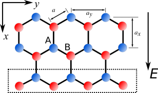
Figure 1: Tight-binding model of graphene. The hexagonal lattice structure is composed of two triangular sublattices labeled as $A$ (blue) and $B$ (red). The dashed line encircles a “zig-zag” row perpendicular to the field direction.

II.2 Recursion relations

To solve the model, we utilize the dynamical mean-field theory (DMFT) ³³ within the Keldysh GF formalism, and ignore the intersite self-energy by the el-ph coupling³⁴. In addition to that we keep the nonequilibrium GFs, the main difference from the equilibrium DMFT is that the lattice summation in the DMFT cannot be performed by a sum over wavevectors due to the bias potential. Although the lattice summation is possible by a brute-force matrix inversion in real-space, a much more efficient algorithm can be used in the spatially uniform limit, as proposed in Ref. 13.

We note that the wavevector component $p_{y}$ perpendicular to the field $E$ is a good quantum number, and we organize the Hamiltonian as depicted in Fig. 1 into zig-zag rows (dashed rectangle, indexed by $\ell$). We consider the hopping within the row parametrized by $p_{y}$, and then exactly treat the inter-row hopping through the self-energy addition ${\bf F}_{\pm}(\omega)$ from the (semi-infinite) upper rows and the lower rows, respectively.

To proceed, we diagonalize the Hamiltonian within the $\ell$-th row with the Fourier transform $d^{\dagger}_{\ell s}(p_{y})=\frac{1}{\sqrt{N_{y}}}\sum_{\bm{r}\in\{\ell s\}}e^{ip_{y}\bm{r}\cdot\bm{\hat{e}}_{y}}d^{\dagger}_{\bm{r}}$, where the summation is limited to all atoms inside the $\ell$-th row and with the sublattice index $s=\pm$ (or $A$/$B$). $N_{y}$ is the number of atoms in a row for normalization. We then obtain the transverse Hamiltonian per momentum $p_{y}$:

$$H_{\text{TB},\perp}(p_{y})=-2\gamma\sum_{\ell}\cos(p_{y}a_{y}/2)d^{\dagger}_{\ell A}(p_{y})d_{\ell B}(p_{y})+\text{H.c.}$$ (6)

The constant $a_{y}=\sqrt{3}a$ is shown in Fig. 1. The longitudinal Hamiltonian is

$$H_{\text{TB},\parallel}(p_{y})=-\gamma\sum_{\ell}d^{\dagger}_{\ell+1,A}(p_{y})d_{\ell B}(p_{y})+\text{H.c.}$$ (7)

Now the problem is reduced to solving an effectively one-dimensional problem parametrized by $p_{y}$, where a central row ($\ell=0$) is connected to two semi-infinite chains with upper ($\ell>0$) and lower ($\ell<0$) rows via $H_{\text{TB},\parallel}(p_{y})$.

Given $p_{y}$, the GFs ${\bf G}^{\lessgtr}(\omega;p_{y})$ at $\ell=0$ are expressed in the $2\times 2$ sublattice space. By denoting the GF on the edge row of the semi-infinite chains as ${\bf F}_{\pm}(\omega;p_{y})$, we construct the (retarded) GF as^{13; 33}

$$\mathbf{G}^{r}(\omega;p_{y})^{-1} =\omega-{\bf h}_{\perp}(p_{y})-\mathbf{\Sigma}^{r}(\omega)$$

$$-\sum_{\alpha=\pm}\bm{v}_{\alpha}^{\dagger}{\mathbf{F}}^{r}_{\alpha}(\omega+\alpha Ea_{x};p_{y})\bm{v}_{\alpha},$$ (8)

with a given local self-energy $\mathbf{\Sigma}^{r}(\omega)$ by using Dyson’s equation¹³. The intra-row Hamiltonian matrix from Eqs. (6) and (5) is

$${\bf h}_{\perp}(p_{y})=\begin{pmatrix}0&-2\gamma\cos(p_{y}a_{y}/2)\\ -2\gamma\cos(p_{y}a_{y}/2)&-Ea/2\end{pmatrix}.$$ (9)

The matrix $\bm{v}_{\pm}$ is to connect the sublattices via hopping

$$\bm{v}_{+}=\bm{v}^{\dagger}_{-}=\begin{pmatrix}0&&\gamma\\ 0&&0\end{pmatrix}.$$ (10)

The GF on the semi-infinite chains $\mathbf{F}^{\lessgtr}_{\alpha}(\omega;p_{y})$ is calculated recursively ¹³. By exploiting the self-similarity between the edge and the next-to-edge rows, we have the relation

$$\mathbf{F}^{r}_{\alpha}(\omega;p_{y})^{-1} =\omega-{\bf h}_{\perp}(p_{y})-\mathbf{\Sigma}^{r}(\omega)$$

$$-\bm{v}_{\alpha}^{\dagger}\mathbf{F}^{r}_{\alpha}(\omega+\alpha Ea_{x};p_{y})\bm{v}_{\alpha}.$$ (11)

Similarly, the lesser GFs can be computed with the Dyson’s equations¹³,

$$\mathbf{G}^{<}(\omega;p_{y}) =\mathbf{G}^{r}(\omega;p_{y})\bigg{[}\bm{\Sigma}^{<}(\omega)$$

$$+\sum_{\alpha=\pm}\bm{v}_{\alpha}^{\dagger}\mathbf{F}^{<}_{\alpha}(\omega+\alpha Ea_{x};p_{y})\bm{v}_{\alpha}\bigg{]}\mathbf{G}^{a}(\omega;p_{y})$$

$$\mathbf{F}_{\alpha}^{<}(\omega;p_{y}) =\mathbf{F}_{\alpha}^{r}(\omega;p_{y})[\bm{\Sigma}^{<}(\omega)$$

$$+\bm{v}_{\alpha}^{\dagger}\mathbf{F}_{\alpha}^{<}(\omega+\alpha Ea_{x};p_{y})\bm{v}_{\alpha}]\mathbf{F}_{\alpha}^{a}(\omega;p_{y}).$$ (12)

We complete the DMFT loop in the usual manner. The local GF is defined as $\mathbf{G}_{\text{loc}}(\omega)=\frac{1}{N_{y}}\sum_{p_{y}}\mathbf{G}(\omega;p_{y})$. Once we have $\mathbf{G}_{\text{loc}}(\omega)$ and $\mathbf{\Sigma}(\omega)$, we construct the (non-interacting) Weiss-field GF $\mathbf{\mathcal{G}}(\omega)$ as

$$\mathbf{\mathcal{G}}^{r}(\omega)^{-1}=\mathbf{G}^{r}_{\text{loc}}(\omega)^{-1}+\mathbf{\Sigma}^{r}(\omega),$$ (13)

for the retarded functions. Then the Weiss-field $\mathbf{\mathcal{G}}(\omega)$ is used to update the self-energy $\mathbf{\Sigma}(\omega)$ which is then used to update the GFs again, as described so far. The procedure is repeated until a convergence is reached with the 1% variation of current between iterations.

The self-energy has the contribution from the fermion baths and the el-ph coupling: $\mathbf{\Sigma}(\omega)=\mathbf{\Sigma}_{\Gamma}(\omega)+\mathbf{\Sigma}_{\text{ph}}(\omega)$. Within the DMFT, the self-energies are diagonal in the sublattice space. The self-energy by the fermion baths (at $\ell=0$) is given as

$$\mathbf{\Sigma}^{r}_{\Gamma}(\omega)=-i\Gamma,\mathbf{\Sigma}^{<}_{\Gamma}(\omega)=-2i\Gamma\left(\begin{array}[]{cc}f_{0}(\omega)&0\\ 0&f_{0}(\omega+Ea/2)\end{array}\right),$$ (14)

with the Fermi-Dirac function at the bath temperature. The bath temperature has been chosen as $T_{\text{bath}}=0.01\gamma\approx 350$ K unless stated otherwise. For the el-ph coupling, we use the approximation that the phonon GFs are not dressed with the self-energy

$$\Sigma^{<}_{\text{ph},ss}(\omega) = g_{\rm ep}^{2}\left[\mathcal{G}^{>}_{ss}(\omega-\omega_{\text{ph}})(N_{\text{ph}}+1)\right.$$ (15)

$$+ \left.\mathcal{G}^{<}_{ss}(\omega+\omega_{\text{ph}})N_{\text{ph}}\right],$$

with $N_{\text{ph}}=1/[\exp(\omega_{\text{ph}}/T_{\rm ph})-1]$ the Bose-Einstein distribution and the phonon temperature $T_{\text{ph}}$. We assume that $\omega_{\text{ph}}\gg T_{\text{ph}}$ with $\omega_{\text{ph}}\sim 1500$ K, and that the renormalization of the phonon is not strong.

This approximation is in line with the semiclassical pictures adopted in previous works ^{5; 6}. For very large electric fields, the physics may be affected by the hot (optical) phonons excited during the transport process. However, this effect is minimized if phonons are strongly coupled with the environmental bath, and lose energy immediately. This assumption is proven relevant when the graphene sample is in contact with a substrate which dissipates energy very efficiently, such as in the case of hexa-boron-nitride²⁷. In Sect. III. E, we estimate the hot-electron temperature $T_{\rm eff}$ for a charge-neutral graphene in the range of $\sim 500$ K, and we expect the phonon temperature $T_{\text{ph}}$ to be significantly lower than $T_{\rm eff}$ and $\omega_{\text{ph}}$.

Using the above formulation, we directly simulate the nonequilibrium steady-state and compute the steady-state current under given electric fields. After the self-consistent calculation is finished, the current density is calculated with the following definition²⁸,

$$J=i\gamma\sum_{p_{y}}\langle d^{\dagger}_{\ell+1,A}(p_{y})d^{\dagger}_{\ell,B}(p_{y})-\text{H.c.}\rangle/a_{y}.$$ (16)

We refer the readers to the literature for more details^{29; 13; 30}.

III Results

III.1 Signature of Landau-Zener tunneling

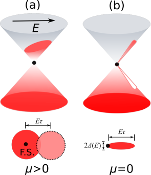
Figure 2: Schematic demonstration of momentum distribution of electric-field-driven graphene (a) off the Dirac point and (b) on the Dirac point. (a) Chemical potential $\mu>0$ and a finite Fermi sphere exists in equilibrium. An electric field displaces the Fermi sphere by $E\tau$ according to the semiclassical picture. (b) $\mu=0$ and the “Fermi sphere” becomes pointlike. In this case, any finite field transport effect is of quantum mechanical nature and should be related to creation of particle-hole pairs. A jetlike distribution for both electrons and holes is created under a finite electric field in the charge-neutral limit.

We first consider the strong-field transport in graphene without optical phonon interaction. The transport behavior is quite different between the cases with zero and finite chemical potential $\mu$. With $\mu>0$, a non-zero Fermi circle exists in the upper band, allowing the semiclassical Boltzmann transport theory to be applied: electric fields displace the Fermi circle in the field direction, as shown in the Fig. 2(a). With a scattering-time $\tau$, the Fermi circle is displaced by $E\tau$. A similar argument can be made for holes in the case of $\mu<0$. With $\mu=0$ the Fermi circle shrinks to a point, as in Fig. 2(b), and the conventional linear-response theory does not apply. Near this point, an electric field excites electrons to the upper band, leaving holes in the lower band. These nonequilibrium excitations are initially driven by the Landau-Zener transition, and the electrons are accelerated by the electric field during the scattering time $\tau$, resulting in a highly anisotropic excitation distribution. Physically, the steady-state current is established when the Landau-Zener tunneling and field-driven acceleration of electrons are balanced by electron-phonon interaction as well as other dephasing mechanisms. The excitation distribution in the momentum space forms streaking lines in the particle and hole cones along the direction of the field. This is a solid-state analog of the Schwinger effect ²³, a particle-antiparticle pair creation by an intense electric field with zero mass gap.

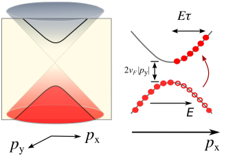
Figure 3: Demonstration of Landau-Zener tunneling in graphene on the Dirac point. When the Dirac cone intersects with a plane of nonzero $p_{y}$, the excitations in the gapped quasi-one-dimensional dispersion relation is understood in terms of the Landau-Zener tunneling. Significant electron-hole pairs are created for $|p_{y}|\lesssim\Delta(E)$.

With an electric field in the $x$ direction, the perpendicular momentum $p_{y}$ is a good quantum number and we analyze the excitations on the dispersion relation on a sliced cone at a fixed $p_{y}$, as shown in Fig. 3. At $p_{y}\neq 0$, the dispersion relation is gapped with the charge gap $2v_{F}|p_{y}|$. The transition of an electron from the lower band to the upper band due to a constant force field is described by the Landau-Zener tunneling with the transition probability $\gamma_{\rm LZ}$ as

$$\gamma_{\text{LZ}}=\exp(-\pi v_{F}p_{y}^{2}/E).$$ (17)

This suggests that electrons only with $|p_{y}|\lesssim\sqrt{E/\pi v_{F}}\equiv\Delta_{0}(E)$ are excited to the upper band [$\Delta_{0}(E)$ is the width of the distribution under electric field $E$] with the subscript $0$ referring to without phonons. On the other hand, the range of excitation of the longitudinal momentum $p_{x}$ is given by the lifetime of the excited electrons. The fermion bath provides the lifetime ^{28; 35} $\tau_{\Gamma}=(2\Gamma)^{-1}$ and the range of $p_{x}$ for excited electrons become $0\lesssim p_{x}\lesssim E\tau_{\Gamma}$. Combining these observations, an ansatz is proposed for the momentum distribution for the excitations as

$$n_{\bm{p}}\propto\theta(\Delta_{0}(E)-|p_{y}|)\theta(E\tau_{\Gamma}-p_{x})\theta(p_{x}),$$ (18)

and the number of excited electrons $n_{\rm ex}$ behaves as

$$n_{\rm ex}\propto\Delta_{0}(E)E\tau_{\Gamma}\propto E^{3/2}/\Gamma.$$ (19)

The excitation of holes has exactly the same distribution as the electrons, with the jet-like excitation on the same side of the momentum. Similar momentum distribution has been proposed in the streaming model ¹², where the Fermi sea is elongated in the direction of the field by $E\tau$. However, in the $\mu=0$ limit, a finite Fermi sea does not exist and this phenomenological approach does not provide any mechanism for the width of the stream.

This simple argument leads to a straightforward prediction of the $I$-$V$ characteristics. In the limit of $E\tau_{\Gamma}\gg\Delta_{0}(E)$, the jet-like distribution is almost completely aligned with the electric field and the averaged velocity is close to $v_{F}$, resulting in $J\propto n_{\text{neq}}v_{F}\propto E^{1.5}\tau_{\Gamma}$, which is verified in Fig. 4. In the absence of the el-ph coupling ($g_{\rm ep}=0$), the $J\propto E^{1.5}$ scaling law is shown (solid lines) with the power greater than 1 as the signature of Landau-Zener mechanism. The inset shows the collapse of data to the form $J\sim E^{1.5}/\Gamma$.

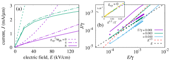
Figure 4: $J-E$ relation of graphene under strong field. (a) Deviations of current from non-interacting case ($g_{\rm ep}=0.0$, dash lines) to $g_{\rm ep}^{2}/\omega_{\text{ph}}=4\gamma$ (dotted dash lines) and $8\gamma$ (solid lines). The damping $\Gamma=0.001\gamma$. The green (purple) lines are with $\mu=0.10\gamma$ ($\mu=0.0\gamma$). (b) The currents with (dots) and without (solid lines) the optical-phonon interactions at different damping parameter $\Gamma$. As damping increases, the range of electric field in which $J\propto E^{1.5}$ holds expands. The inset shows the current as a function of $E^{1.5}/\Gamma$ for a variety of $\Gamma=0.001,0.003,0.005,0.007,0.100$. In (b), $g_{\rm ep}^{2}/\omega_{\text{ph}}=4\gamma$ for dots. Optical phonon frequency $\omega_{\text{ph}}$ is $0.05\gamma$. In all plots in this paper, $\gamma$ is set to $3$ eV.

When the optical phonon interaction is turned on ($g_{\rm ep}\neq 0$), the superlinear $JE$ relation becomes marginally sublinear. The strongly inelastic scattering by optical phonons reduces the current, as shown in Fig. 4(a). It is interesting that the window for the $J\sim E^{3/2}$ shrinks as the damping $\Gamma$ is reduced as shown in Fig. 4(b), whereas it may be naively expected that a clean limit ($\Gamma\to 0$) may preserve the peculiar fractional power law. This can be explained as follows. In the small $\Gamma$ limit, the electrons lifetime increases and the energy increase due to the acceleration $v_{F}(E\tau_{\Gamma})$ reaches the optical phonon threshold $\hbar\omega_{\rm ph}$ at a smaller field $E$. This is consistent with the findings that the superlinear behavior is observed in low-mobility devices under dc-electric field ²⁰, as well as graphene samples excited by THz electric pulses ¹⁸. In the clean limit, the observed $JE$ relations remain close to linear in strong-field transport experiments ^{6; 27}.

III.2 Steady-state current at large fields

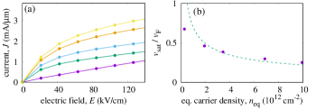
Figure 5: (a) $J$-$E$ curve for different chemical potential $\mu$. As system is taken away from the Dirac point, current increases and shows the saturating behavior under high-field. The $J$-$E$ curves in (a) have chemical potentials $\mu=0.0,0.05,0.07,0.10,0.12$ from bottom to top. (b) Computed relation (dots) $v_{\rm sat}\propto 1/\sqrt{n_{\rm eq}}$ between the saturated velocity $v_{\text{sat}}$ and the equilibrium charge density $n_{\text{eq}}$. This is consistent with the semiclassical formula (20) (dashed line). $\Gamma=0.003\gamma$, $\omega_{\text{ph}}=0.05\gamma$, and $g_{\text{ep}}^{2}/\omega_{\text{ph}}=8\gamma$.

Now we study the effect of optical phonon interaction more closely. Recently, the phenomena of current saturation have attracted intense interest.^{36; 7; 10; 11; 8} It is found that the current saturation in graphene at high electric field depends on the optical phonon frequency $\omega_{\text{ph}}$ and equilibrium current carrier density $n_{\text{eq}}$. The former is a parameter independent of electric control, and the latter is controlled through the chemical potential $\mu$. We are mostly interested in how the graphene behaves under different chemical potentials, especially when it is close to the Dirac point $\mu=0$. Figure 5 systematically shows calculated $J\sim E$ relations with a set of realistic parameters. In graphene, the tight-binding hopping parameter $\gamma\approx 3$ eV and the optical-phonon frequency $\omega_{\text{ph}}=0.05\gamma\approx 150$ meV. These values are close to the empirical parameter used in previous works ^{12; 8; 11}.

In Fig. 5, the electronic current generally shows the tendency to saturate under high electric fields in the samples with relatively high equilibrium electron density. Previous semi-classical analyses ^{5; 12} have assumed that Fermi sphere is shifted by $\hbar\omega_{\text{ph}}/v_{F}$, leading to an empirical formula of the saturated velocity,

$$v_{\text{sat}}=\frac{1}{\sqrt{\pi}}\frac{\omega_{\text{ph}}}{\sqrt{n_{\text{eq}}}},$$ (20)

where $n_{\text{eq}}$ is the equilibrium current carrier density. While this expression has been confirmed experimentally, the formula obviously breaks down when $\omega_{\text{ph}}$ is too large or $n_{\text{eq}}$ is too small, since $v_{\text{sat}}$ can never be greater than $v_{F}$. Our main interest is in the regime the approximation fails. Our calculations do not show true saturation of current and we derive the drift velocity according to a phenomenological model ¹¹:

$$v_{d}=\frac{\chi_{0}E}{1+\chi_{0}E/v_{\text{sat}}},$$ (21)

where $\chi_{0}$ is the zero-field mobility. As verified in Fig. 5(b), the extracted $v_{\text{sat}}$ follows $1/\sqrt{n_{\text{eq}}}$ relation until the Dirac point is reached. Interestingly, recent measurements using short bias pulses ⁸ reported a similar range of the maximum drift velocity $v_{d}\approx 0.5\times v_{F}$ close to the Dirac point.

III.3 Evolution of momentum distribution under external field

To further understand the steady-state current due to the optical phonon scattering, we look at the evolution of momentum distribution $n_{\bm{p}}$ under electric fields. The formulation is detailed in Appendix A. At $\mu>0$ a finite Fermi sea exists around the center of the Dirac cone, as shown in Fig. 6 for the current and momentum distributions. The Fermi sea is shifted along the field-direction when electric field is applied. However, at high electric fields, the Fermi sea stops to shift due to the strong relaxation by the optical phonons when electrons lose their excess energy to phonon baths. This is consistent with the semi-classical Boltzmann transport calculations.⁹

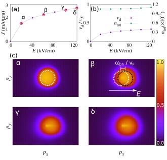
Figure 6: Charge excitations and the momentum distribution of electrons under electric fields in the off-Dirac-point graphene. (a) Saturation of current under electric fields and (b) drift velocity $v_{d}$ and total current carriers number $n_{\text{tot}}$ under electric fields. The $v_{d}$ saturates like current, and $n_{\text{tot}}$ is almost unchanged. (c) Momentum distributions of electrons at $\mu=0.1\gamma$. Fermi sea is shifted at small electric fields. Its displacement is nearly unchanged at high fields. Near ${\bf p}=0$, a faint signature of the Schwinger effect can be seen in the panels $\gamma$ and $\Delta$.

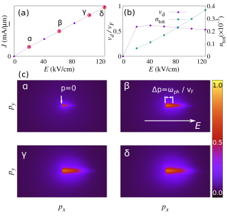
Figure 7: Charge excitations and the momentum distribution of electrons under electric fields in the on-Dirac-point graphene. (a) Current which scales linearly with electric field. (b) Drift velocity $v_{d}$ and total number of current carriers $n_{\text{tot}}$. The drift velocity overshoots and then decreases due to optical phonon emission, and the total number of excitations $n_{\text{tot}}$ increases monotonically with $E$. (c) Momentum distribution of electrons (upper band). At high fields, the center of excitation distribution is at the momentum $p_{x}=\Delta p\approx\omega_{\rm ph}/v_{F}$. The distribution of holes is essentially identical.

At $\mu=0$, as shown in Fig. 7(a), the current increases almost linearly without saturation. To investigate the origin, we plot the electron excitation $n_{\rm ex}$ and the drift velocity $v_{d}$ calculated by

$$v_{d}=v_{F}\frac{\int_{|{\bm{p}}|<\Lambda_{p}}n({\bm{p}})\!\cos\theta d^{2}{\bm{p}}}{\int_{|{\bm{p}}|<\Lambda_{p}}n({\bm{p}})d^{2}{\bm{p}}},$$ (22)

with the angle $\theta$ between the field and momentum vectors, and the large momentum cutoff $\Lambda_{p}$. It is clear that the drift velocity saturates at small field and the main contribution to the current $J=n_{\rm ex}v_{d}$ is due to the electron excitations linearly proportional to the field $E$. We emphasize that the drift velocity is evaluated by dividing the current by the excited charge out of neutrality, instead of the equilibrium charge $n_{\rm eq}$ as often used in experimental estimates.

Let us investigate more into the excitations in the momentum space. Figure 7(c) shares the characteristics proposed in Eq. (18). However, coupling to the inelastic phonons results in important differences. First, as the electric field increases, the length of the jet stops growing but saturates to the length related to the phonon frequency, $(p_{x})_{\rm max}\sim 2\omega_{\rm ph}/v_{F}$ with the center of distribution at $\omega_{\rm ph}/v_{F}$. Therefore, $E\tau_{\Gamma}$ in Eq. (18) is replaced by $2\omega_{\rm ph}/v_{F}$. Second, the width of the distribution $\Delta(E)$ no longer follows the Landau-Zener form $\Delta_{0}(E)\propto\sqrt{E}$. As the distribution saturates, the width $\Delta(E)$ gets smeared due to the local scattering by optical phonons, which can be summarized as

$$n_{\bm{p}}\propto\theta(\Delta(E)-|p_{y}|)\theta(2\omega_{\rm ph}/v_{F}-p_{x})\theta(p_{x}).$$ (23)

Due to the smearing of the momentum distribution with stronger el-ph scattering at high fields, the drift velocity is slightly reduced with a wider angular distribution in Eq. (22), as shown in Fig. 7(b).

We now discuss the role of the electron-electron scattering in the $I$-$V$ characteristics considered in this section^{12; 37}. We expect that the qualitative nature of the charge excitations discussed above remain robust against the $e$-$e$ interactions. Due to the momentum and energy conservation in the Coulomb scattering³⁸ in graphene, the phase space in the scattering process is strongly limited. Out of a jetlike distribution [see Fig. 7(c)], intra-band scattering events with collinear incoming momenta will scatter into another pair of collinear momenta moving in the same direction, preserving the strong anisotropy of the distribution. Other interband e-e interaction processes, such as carrier multiplication and the Auger process, should also be suppressed³⁸ in this case since they involve scattering electrons (holes) into fully occupied (empty) states. This argument does not apply in ultrafast measurements ^{39; 22}, in which electrons incoming with opposite momenta induced by oscillating field can scatter into any outgoing direction and relax to an isotropic momentum distribution.

III.4 Energy dissipation

To understand the strong-field $IV$ relation at Dirac point with optical-phonon interaction, we look into the energy conservation law: the electric power $JE$ is equal to the dissipation rate. In the case when the optical phonon scattering dominates at large $E$, the scattering rate is $\tau^{-1}_{\text{ph}}=-\text{Im}(\Sigma^{<}_{\text{ph}}-\Sigma^{>}_{\text{ph}})$ and each scattering between an electron and optical phonon reduces the electron energy by $\hbar\omega_{\text{ph}}$. So the dissipation rate of nonequilibrium excitations is $n_{\text{ex}}\omega_{\text{ph}}\tau^{-1}_{\text{ph}}$. The system at finite temperature can have a small equilibrium current carrier density $n_{\text{eq}}$, but we will concentrate on the $\mu=0$ case where $n_{\text{eq}}\approx 0$, and the total electron density $n_{\text{tot}}\approx n_{\text{ex}}$. We then have

$$JE =n_{\text{ex}}\omega_{\text{ph}}\tau^{-1}_{\text{ph}}+\Theta_{\Gamma}.$$ (24)

The $\Theta_{\Gamma}$ is the dissipation rate due to fermion reservoirs. In the following, we will focus on the case where $\Theta_{\Gamma}$ is physically negligible. This approximation is tested in Fig. 8(a), with $\tau_{\text{ph}}$ being the scattering rate at $\omega=0$.

The el-ph scattering rate $\tau^{-1}_{\rm ph}$ is given as a convolution of electron and phonon Green’s functions and is thus proportional to the electron density. We show that

$$\tau_{\text{ph}}^{-1}=\alpha n_{\text{ex}},$$ (25)

as in Fig. 8(b), with the coefficient $\alpha$ explicitly calculated in Appendix B. It is shown both theoretically and numerically that $\alpha$ is proportional to $g_{\text{ep}}^{2}$, given by $\alpha=\pi A_{c}g_{\text{ep}}^{2}/2\omega_{\text{ph}}$. The parameter $\alpha$ is independent of the electric field, and it can be evaluated experimentally at zero field by the line broadening of the electrons due to phonons.

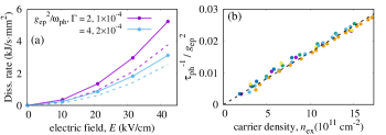
Figure 8: (a) Energy dissipation rate in the presence of optical phonons with frequency $\omega_{\text{ph}}$, and (b) the observed $\tau^{-1}_{\text{ph}}\propto n_{\text{ex}}$ relation. In (a), the dots are total dissipation rate $JE$, and the dashed lines are the dissipation rates due to optical phonon emission, predicted by Eq. (24). The predicted dissipation rate does not deviate much from the numerically calculated values at strong optical phonon interaction. We have assumed $\hbar\omega_{\text{ph}}\approx 150$ meV and $\Gamma\sim 0.0001\gamma$, which corresponds to $\tau^{-1}_{\Gamma}\sim 1\text{ ps}^{-1}$ assuming $\gamma=3$ eV. The $g_{\rm ep}^{2}/\omega_{\text{ph}}\sim 2\gamma$ leads to $\tau^{-1}_{\text{ph}}$ being in the order of $10\text{ ps}^{-1}$. In (b), the linear relation of $\tau^{-1}=\alpha n_{\text{ex}}$ is tested for a variety of interaction strengths $g^{2}_{\text{ep}}/\omega_{\text{ph}}=2,4,8,12,16$ and $\Gamma=0.0001,0.0002,0.001$.

A crucial step to understand the linear $J$-$E$ relation is the relation $n_{\rm ex}\propto E$. We may relate the el-ph scattering rate $\tau_{\rm ph}^{-1}$ in two different ways. One can argue that, in the high-field limit, the frequency of the el-ph scattering is determined by how fast the electron energy gained by the $E$-field reaches the optical phonon frequency, that is, with the average energy excitation at momentum $\Delta p$ [see Fig. 7(c)] given as $v_{F}\Delta p=v_{F}E\tau_{\rm ph}\sim\omega_{\rm ph}$, which leads to $\tau_{\rm ph}^{-1}\sim v_{F}E/\omega_{\rm ph}$. This result is consistent with a more careful analysis based on Eq. (24). In the saturated drift velocity limit, the current $J$ in the energy-conservation relation (24) is replaced by $n_{\text{ex}}v_{\text{sat}}$. We then re-derive

$$\tau^{-1}_{\text{ph}}=v_{\text{sat}}E/\omega_{\text{ph}}.$$ (26)

after eliminating $n_{\text{ex}}$.

By eliminating $\tau_{\rm ph}^{-1}$ from the Eqs. (25) and (26), we obtain

$$n_{\text{ex}}=\frac{v_{\text{sat}}}{\alpha\omega_{\text{ph}}}E,$$ (27)

and the current-field relation immediately follows close to the Dirac point (after restoring the physical constants)

$$J\approx n_{\text{ex}}v_{\text{sat}}=\frac{e^{2}v_{\text{sat}}^{2}}{{\alpha\hbar\omega_{\text{ph}}}}E.$$ (28)

The saturated velocity has weak dependence on the electric field in the strong field limit. This result shows that the main electric field dependence originates from the charge excitation proportional to $E$. The formula is tested with numerical results in Fig. 9. The parameter $v_{\text{sat}}$ is extracted from numerical calculations. In experiments, the formula may provide a way to extract $v_{\text{sat}}$ from the measured $I$-$E$ relation in the presence of both optical phonon emission and Landau-Zener tunneling. Using the relation $n_{\rm ex}\tau_{\rm ph}=\alpha^{-1}$, the $J$-$E$ relation can be cast in the usual Drude form as $J=(n_{\text{ex}}\tau_{\text{ph}}/m^{*})E$ with the effective mass $m^{*-1}\sim v_{\text{sat}}^{2}/\hbar\omega_{\text{ph}}$ for the driven Dirac particles, whose kinetic energies are of the magnitude of $\hbar\omega_{\text{ph}}$.

We reemphasize that, despite its similarity to the Ohmic law of simple metals, the origin of the above linear $J$-$E$ relation is very different. In a simple metal, while the carrier density $n_{\text{eq}}$ is weakly perturbed by the electric fields, the drift velocity $v_{d}$ is proportional to the $E$-field. For the Dirac electrons in graphene, however, the role of the electric field is reversed: $v_{d}\approx v_{\text{sat}}\sim v_{F}$ at saturation while the nonequilibrium carriers density $n_{\text{ex}}\propto E$.

Figure 9: $J$-$E$ relation of Dirac electron compared with the theoretical prediction. The theoretical $J$-$E$ relation (28) is compared against the numerical data (dots). $v_{\text{sat}}\sim 0.5v_{F}$ in the formula is extracted from the numerical data. The theory correctly predicts that the power of $J$-$E$ relation is close to one, and quantitatively matches the numerical data. Bath temperature is set to 35K in this calculation.

III.5 Effective temperature

A nonequilibrium effective temperature in a dc-transport system is the direct consequence of the balance between the electric power and the energy dissipation. Here, we follow the procedure in Ref. 30 to define the effective temperature from the nonequilibrium distribution function

$$f_{\text{loc}}(\omega)=-\frac{\text{Im}G_{\text{loc}}^{<}(\omega)}{2\text{Im}G_{\text{loc}}^{r}(\omega)}.$$ (29)

The nonequilibrium distribution function usually has a different functional form from the equilibrium Fermi-Dirac distribution in which temperature is a well-defined parameter. To obtain a comparable nonequilibrium temperature parameter, we define the effective $T_{\text{eff}}$ from the first moment of the distribution function,

$$\frac{\pi^{2}}{6}T^{2}_{\text{eff}}=\int\omega\left[f_{\text{loc}}(\omega)-\theta(-\omega+\mu)\right]d\omega.$$ (30)

$\Theta(\omega)$ is the Heaviside step function. This definition is consistent with the Fermi-Dirac distribution at an equilibrium temperature.

With this definition, we plot the effective temperature in Fig. 10. In the case of $g_{\rm ep}=0$, effective temperature of the off-Dirac-point graphene is always higher than that of the on-Dirac-point system. This is because higher current carrier density results in higher current. The system with more current-carrying excitations create more Joule heating thereby the temperature is also higher. However, this is dramatically changed when optical phonon interaction is considered. In this case, the system with higher electron density still has higher electric current for all electric fields. However, at higher electric fields, the effective temperature of the off-Dirac-point system falls below the temperature of the Dirac-electron system.

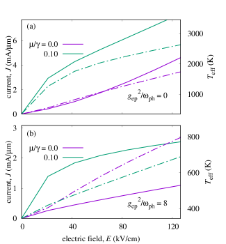
Figure 10: Current and effective temperature of graphene (a) on and (b) off Dirac point. $\Gamma=0.001\gamma$. The solid lines are currents, while dot-dashed lines are nonequilibrium effective temperature calculated under different electric fields. When optical-phonon coupling is switched off, the sample with $\mu=0.10t$ (away from the Dirac point) shows higher effective temperature due to higher current as well as Joule heating; however, optical phonon emission results in current saturation as discussed above, and the behavior of $T_{\text{eff}}$ becomes more complicated, with a crossover of $T_{\text{eff}}$ occurring at finite electric fields.

To explain this crossover behavior, we note that the effective temperature is the measure of the amount of excitations. As the electric field increases, the el-ph coupling overrides the relaxation by the fermion baths. As we argued above, the energy relaxation by phonons is proportional to the electronic charge density, and at non-zero $\mu$, the finite Fermi surface makes the relaxation more efficient, thereby cools the electron temperature more effectively than at the $\mu=0$ limit. The effective temperature is predicted to be in the range of 400-800 K in the realistic range of the electric field.^{40; 41; 42; 43; 44} We note that recent works ^{45; 27} have reported much higher hot-electron temperatures in graphene systems.

IV Conclusion

We have demonstrated that Dirac electrons in graphene become excited in a non-trivial manner and lead to a marginally linear dependence of electric current under a dc electric field, through microscopic calculations based on the Keldysh Green’s-function theory. Inelastic scattering by optical phonons is shown to be crucial to produce the nonequilibrium charge excitation population $n_{\rm ex}$ and the electric current linearly proportional to the external field, close to a Dirac point, as summarized as

$$J\approx\frac{e^{2}v_{\text{sat}}^{2}}{\alpha\hbar\omega_{\text{ph}}}E,$$ (31)

with the saturated drift velocity $v_{\rm sat}$, the optical phonon frequency $\omega_{\rm ph}$, and the coefficient $\alpha$ proportional to the el-ph coupling constant. The mechanism for this apparent Ohmic $I$-$V$ characteristics in the Dirac limit is different from the conventional Drude model in that the linear dependence of the electric field comes from the nonequilibrium charge density instead of the drift velocity. This linear $JE$ relation without saturation close to the Dirac point has been observed in clean graphene encapsulated by the hexa-boron-nitrides ^{27; 46}. Away from the Dirac charge-neutrality point, the conventional Boltzmann transport is recovered with the tendency for the current saturation with where the drift velocity is proportional to $\omega_{\rm ph}/n_{\rm eq}^{1/2}$ with the equilibrium charge density $n_{\rm eq}$.

The electron-hole excitations at the charge-neutral point ($\mu=0$) are strongly anisotropic in the momentum space with the excited electrons and holes staying in the momentum regime of the same direction, an analog of the Schwinger effect in a solid state system. The inter-band creation of electron-hole pairs poses possibilities for optical applications. The continuous excitation energy up to the optical phonon energy of $\sim 150$ meV can be used for infra-red optical devices, without any lower threshold. Most intriguing is the change of the coupling of the electron-hole pairs to photons upon switching of the bias. Close to the Dirac point, the wavefunction under dc electric field acquires extra phase oscillation due to the potential gradient which can strongly suppress the photon-generation. When the electric-field is turned off, the electron wavefunction becomes a plane-wave and the coupling to the photon field enhances roughly by the factor proportional to the length of the sample. This mechanism may be utilized in a fast-switching IR-optic diode.

V Acknowledgements

JL acknowledges the computational support from the Center for Computational Research (CCR) at University at Buffalo. We thank Jonathan P. Bird, Takuya Higuchi, Alexander Khaetskii, Huamin Li and Christian Heide for their helpful discussions throughout the study.

Appendix A Momentum distribution of electrons

To compute the momentum distribution of electrons, we note that $\mathbf{n}_{\bm{p}}=-i\mathbf{G}^{<}_{\bm{p}}(t,t)=-i\sum_{\bm{r}}\exp(i\bm{p}\cdot\bm{r})\mathbf{G}^{<}_{\bm{r}\bm{0}}(t,t)$. We have used matrix-valued Green’s functions and $\mathbf{n}_{\bm{p},ss^{\prime}}=-iG^{<}_{\bm{p},ss^{\prime}}(t,t)$. Using the time-translational invariance of the Green’s functions, time $t$ can be fixed as $0$, so the momentum distribution is calculated as

$$\mathbf{n}_{\bm{p}} =-i\sum_{\bm{r}}\exp(i\bm{p}\cdot\bm{r})\int\frac{d\omega}{2\pi}\mathbf{G}^{<}_{\bm{r}\bm{0}}(\omega)$$

$$=-i\sum_{\bm{r}}\exp(i\bm{p}\cdot\bm{r})\int\frac{d\omega}{2\pi}\sum_{\bm{r}^{\prime}}\mathbf{G}^{r}_{\bm{r}\bm{r}^{\prime}}(\omega)\mathbf{\Sigma}^{<}(\omega+\bm{r}^{\prime}\cdot\bm{E})$$

$$\quad\times\mathbf{G}^{a}_{\bm{r}^{\prime}\bm{0}}(\omega),$$ (32)

where $\mathbf{\Sigma}^{<}(\omega)=\mathbf{\Sigma}_{\Gamma}^{<}(\omega)+\mathbf{\Sigma}_{\text{ph}}^{<}(\omega)$ is the total lesser self energy, including components from both fermion reservoirs and optical phonon baths. Now we shift $\omega\to\omega-\bm{r}^{\prime}\cdot\bm{E}$, and notice that $\mathbf{G}^{r}_{\bm{r+a}\bm{r^{\prime}+a}}(\omega)=\mathbf{G}^{r}_{\bm{r}\bm{r}^{\prime}}(\omega+\bm{a}\cdot\bm{E})$, with $\bm{r},\bm{r}^{\prime}$ and $\bm{a}$ being lattice vectors. Therefore the formula is reduced to

$$\mathbf{n}_{\bm{p}} =-\frac{i}{2\pi}\int d\omega\sum_{\bm{r}\bm{r}^{\prime}}\exp(i\bm{p}\cdot\bm{r})\mathbf{G}^{r}_{\bm{r}\bm{r}^{\prime}}(\omega-\bm{r}^{\prime}\cdot\bm{E})\mathbf{\Sigma}^{<}(\omega)$$

$$\quad\times\mathbf{G}^{a}_{\bm{r}^{\prime}\bm{0}}(\omega-\bm{r}^{\prime}\cdot\bm{E})$$

$$=-\frac{i}{2\pi}\int d\omega\sum_{\bm{r}\bm{r}^{\prime}}\exp(i\bm{p}\cdot(\bm{r}-\bm{r}^{\prime}))\mathbf{G}^{r}_{\bm{r}-\bm{r}^{\prime},\bm{0}}(\omega)\mathbf{\Sigma}^{<}(\omega)$$

$$\quad\times[\exp(-i\bm{p}\cdot\bm{r}^{\prime})\mathbf{G}^{r}_{-\bm{r}^{\prime}\bm{0}}(\omega)]^{\dagger}$$

$$=-\frac{i}{2\pi}\int d\omega\mathbf{G}^{r}_{\bm{p}}(\omega)\mathbf{\Sigma}^{<}(\omega)\mathbf{G}^{a}_{\bm{p}}(\omega),$$ (33)

where we have defined $\mathbf{G}^{r}_{\bm{p}}(\omega)=\sum_{\bm{r}}\exp(i\bm{p}\cdot\bm{r})\mathbf{G}^{r}_{\bm{r}\bm{0}}(\omega)$. In practical calculations, we firstly compute $\mathbf{G}^{r}_{\bm{r}\bm{0}}(\omega)$ and Fourier transform them to $\mathbf{G}^{r}_{\bm{p}}(\omega)$ in momentum space. Then $n_{\bm{p}}$ is calculated by evaluating the integral in (33). Finally, to interpret the result $\mathbf{n}_{\bm{p}}$, we should expand it in terms of equilibrium diagonalized basis²,

$$\psi_{\pm,\bm{p}} =\frac{1}{\sqrt{2}}\begin{pmatrix}e^{-i\theta_{\bm{p}}/2}\\ \pm e^{i\theta_{\bm{p}}/2}\end{pmatrix},$$

$$\text{with}\quad\exp(i\theta_{\bm{p}})=\epsilon_{\bm{p}}/|\epsilon_{\bm{p}}|,$$ (34)

with $\epsilon_{\bm{p}}$ given by

$$\epsilon_{\bm{p}}=-\gamma\left(1+2e^{-ip_{x}a_{x}}\cos\frac{p_{y}a_{y}}{2}\right).$$ (35)

We define unitary transformation $U_{\bm{p}}=\begin{pmatrix}\psi_{+,\bm{p}}&\psi_{-,\bm{p}}\end{pmatrix}$, and transform the $\mathbf{n}_{\bm{p}}$,

$$\mathbf{\tilde{n}}_{\bm{p}}=U_{\bm{p}}^{\dagger}\mathbf{n}_{\bm{p}}U_{\bm{p}}$$ (36)

Then the particle numbers for upper/lower bands are $\mathbf{\tilde{n}}_{\bm{p},++}$ and $\mathbf{\tilde{n}}_{\bm{p},--}$. These equations will be useful to calculate the nonequilibrium momentum distribution.

Appendix B Derivation of Eq. (25), $\tau^{-1}_{\text{ph}}=\alpha n_{\text{ex}}$

In our self-consistent calculations, the 2nd-order electron self-energy by the optical phonon interaction is given by

$$\Sigma^{\lessgtr}_{\text{ph}}(\omega) \approx g_{\rm ep}^{2}G^{\gtrless}(\omega\mp\omega_{\text{ph}}),$$ (37)

with coupling constant $g_{\rm ep}$. The approximation is made due to the nearly empty optical phonon bath, where phonons are rarely excited before the nonequilibrium excitations having energy close to the optical phonon energy. Then the scattering rate at $\omega=0$ becomes

$$\tau_{\text{ph}}^{-1} =-ig_{\rm ep}^{2}[G^{<}(\omega_{\text{ph}})-G^{>}(-\omega_{\text{ph}})]$$

$$=2\pi g_{\rm ep}^{2}[A(\omega_{\text{ph}})f_{\text{loc}}(\omega_{\text{ph}})+A(-\omega_{\text{ph}})\left(1-f(-\omega_{\text{ph}})\right)]$$

$$=4\pi g_{\rm ep}^{2}\rho(\omega_{\text{ph}}),$$ (38)

with the particle-hole symmetry in the spectral function $A(\omega)=A(-\omega)$ and the distribution function $f_{\rm loc}(\omega)=1-f_{\rm loc}(-\omega)$ at the charge-neutrality point $\mu=0$. $\rho(\omega)=A(\omega)f_{\text{loc}}(\omega)$ is the occupation density of electrons at frequency $\omega$. As a first-order approximation, we again assume the jet-like distribution $n_{\bm{p}}$ is uniform within a thin rectangular box aligned in the field-direction and zero outside the box, as in Eq. (23). Note the number of excited electrons in the energy interval $[\omega,\omega+d\omega]$ should be

$$\rho(\omega)d\omega\propto\int_{\omega<v_{F}p<\omega+d\omega}n_{\bm{p}}d^{2}\bm{p}.$$ (39)

This rectangle-shaped momentum distribution results in the uniform $\rho(\omega)\approx\rho(\omega_{\text{ph}})$ when $|\omega|\lesssim 2\omega_{\text{ph}}$ and zero otherwise. Then we have

$$n_{\text{ex}}=2\int{d\omega\rho(\omega)}/A_{c}\approx 4g_{v}\rho(\omega_{\text{ph}})\omega_{\text{ph}}/A_{c},$$ (40)

with $g_{v}=2$ counting the valley degrees of freedom and $A_{c}=\frac{3\sqrt{3}}{2}a^{2}$ being the area of unit cell. The prefactor $2$ is included to count both electrons and holes. By comparing (38) and (40), we have

$$\tau_{\text{ph}}^{-1} =\alpha n_{\text{ex}},\quad\text{with }\alpha=\frac{\pi g_{\rm ep}^{2}A_{c}}{2\omega_{\text{ph}}}.$$ (41)

References

- Novoselov et al. (2004) K. S. Novoselov, A. K. Geim, S. V. Morozov, D. Jiang, Y. Zhang, S. V. Dubonos, I. V. Grigorieva, and A. A. Firsov, Science 306, 666 (2004).
- Neto et al. (2009) A. C. Neto, F. Guinea, N. M. Peres, K. S. Novoselov, and A. K. Geim, Rev. Mod. Phys. 81, 109 (2009).
- Das Sarma et al. (2011) S. Das Sarma, S. Adam, E. H. Hwang, and E. Rossi, Rev. Mod. Phys. 83, 407 (2011).
- Moser et al. (2007) J. Moser, A. Barreiro, and A. Bachtold, Appl. Phys. Lett. 91, 163513 (2007).
- Meric et al. (2008) I. Meric, M. Y. Han, A. F. Young, B. Ozyilmaz, P. Kim, and K. L. Shepard, Nat. Nanotechnol. 3, 654 (2008).
- Barreiro et al. (2009) A. Barreiro, M. Lazzeri, J. Moser, F. Mauri, and A. Bachtold, Phys. Rev. Lett. 103, 076601 (2009).
- Dorgan et al. (2010) V. E. Dorgan, M.-H. Bae, and E. Pop, Appl. Phys. Lett. 97, 082112 (2010).
- Ramamoorthy et al. (2015) H. Ramamoorthy, R. Somphonsane, J. Radice, G. He, C.-P. Kwan, and J. Bird, Nano Lett. 16, 399 (2015).
- Chauhan and Guo (2009) J. Chauhan and J. Guo, Appl. Phys. Lett. 95, 023120 (2009).
- DaSilva et al. (2010) A. M. DaSilva, K. Zou, J. K. Jain, and J. Zhu, Phys. Rev. Lett. 104, 236601 (2010).
- Perebeinos and Avouris (2010) V. Perebeinos and P. Avouris, Phys. Rev. B 81, 195442 (2010).
- Fang et al. (2011) T. Fang, A. Konar, H. Xing, and D. Jena, Phys. Rev. B 84, 125450 (2011).
- Li et al. (2015) J. Li, C. Aron, G. Kotliar, and J. E. Han, Phys. Rev. Lett. 114, 226403 (2015).
- Zener (1932) C. Zener, Proc. R. Soc. A 137, 696 (1932).
- Danneau et al. (2008) R. Danneau, F. Wu, M. F. Craciun, S. Russo, M. Y. Tomi, J. Salmilehto, A. F. Morpurgo, and P. J. Hakonen, Phys. Rev. Lett. 100, 196802 (2008).
- Kao et al. (2010) H. C. Kao, M. Lewkowicz, and B. Rosenstein, Phys. Rev. B 82, 035406 (2010).
- Miao et al. (2007) F. Miao, S. Wijeratne, Y. Zhang, U. C. Coskun, W. Bao, and C. N. Lau, Science 317, 1530 (2007).
- Oladyshkin et al. (2017) I. V. Oladyshkin, S. B. Bodrov, Y. A. Sergeev, A. I. Korytin, M. D. Tokman, and A. N. Stepanov, Phys. Rev. B 96, 155401 (2017).
- Rosenstein et al. (2010) B. Rosenstein, M. Lewkowicz, H. C. Kao, and Y. Korniyenko, Phys. Rev. B 81, 041416 (2010).
- Vandecasteele et al. (2010) N. Vandecasteele, A. Barreiro, M. Lazzeri, A. Bachtold, and F. Mauri, Phys. Rev. B 82, 045416 (2010).
- Kané et al. (2015) G. Kané, M. Lazzeri, and F. Mauri, J. Phys. Condens. Matter 27, 164205 (2015).
- Higuchi et al. (2017) T. Higuchi, C. Heide, K. Ullmann, H. B. Weber, and P. Hommelhoff, Nature 550, 224 EP (2017).
- Schwinger (1951) J. Schwinger, Phys. Rev. 82, 664 (1951).
- Dóra and Moessner (2010) B. Dóra and R. Moessner, Phys. Rev. B 81, 165431 (2010).
- Allor et al. (2008) D. Allor, T. D. Cohen, and D. A. McGady, Phys. Rev. D 78, 096009 (2008).
- Fillion-Gourdeau and MacLean (2015) F. m. c. Fillion-Gourdeau and S. MacLean, Phys. Rev. B 92, 035401 (2015).
- Yang et al. (2018) W. Yang, S. Berthou, X. Lu, Q. Wilmart, A. Denis, M. Rosticher, T. Taniguchi, K. Watanabe, G. Fève, Berroir, et al., Nat. Nanotechnol. 13, 47 (2018).
- Han (2013) J. E. Han, Phys. Rev. B 87, 058119 (2013).
- Han and Li (2013) J. E. Han and J. Li, Phys. Rev. B 88, 075113 (2013).
- Li et al. (2017) J. Li, C. Aron, G. Kotliar, and J. E. Han, Nano Lett. (2017).
- Hwang and Das Sarma (2008) E. H. Hwang and S. Das Sarma, Phys. Rev. B 77, 115449 (2008).
- Pietronero et al. (1980) L. Pietronero, S. Strässler, H. R. Zeller, and M. J. Rice, Phys. Rev. B 22, 904 (1980).
- Aoki et al. (2014) H. Aoki, N. Tsuji, M. Eckstein, M. Kollar, T. Oka, and P. Werner, Rev. Mod. Phys. 86, 779 (2014).
- Georges et al. (1996) A. Georges, G. Kotliar, W. Krauth, and M. J. Rozenberg, Rev. Mod. Phys. 68, 13 (1996).
- Mitra and Millis (2008) A. Mitra and A. J. Millis, Phys. Rev. B 77, 220404 (2008).
- Shishir et al. (2009) R. Shishir, D. Ferry, and S. Goodnick, Journal of Physics: Conference Series 193, 012118 (2009).
- Li et al. (2010) X. Li, E. Barry, J. Zavada, M. B. Nardelli, and K. Kim, Appl. Phys. Lett. 97, 082101 (2010).
- Brida et al. (2013) D. Brida, A. Tomadin, C. Manzoni, Y. J. Kim, A. Lombardo, S. Milana, R. R. Nair, K. Novoselov, A. C. Ferrari, G. Cerullo, et al., Nat. Comm. 4, 1987 (2013).
- Malic et al. (2017) E. Malic, T. Winzer, F. Wendler, S. Brem, R. Jago, A. Knorr, M. Mittendorff, J. König-Otto, T. Plötzing, D. Neumaier, et al., Ann. Phys. 529 (2017).
- Freitag et al. (2010) M. Freitag, H.-Y. Chiu, M. Steiner, V. Perebeinos, and P. Avouris, Nat. Nanotechnol. 5, 497 (2010).
- Bae et al. (2010) M.-H. Bae, Z.-Y. Ong, D. Estrada, and E. Pop, Nano Lett. 10, 4787 (2010).
- Bae et al. (2011) M.-H. Bae, S. Islam, V. E. Dorgan, and E. Pop, ACS Nano 5, 7936 (2011).
- Luxmoore et al. (2013) I. J. Luxmoore, C. Adlem, T. Poole, L. Lawton, N. Mahlmeister, and G. R. Nash, Appl. Phys. Lett. 103, 131906 (2013).
- Beechem et al. (2016) T. E. Beechem, R. A. Shaffer, J. Nogan, T. Ohta, A. B. Hamilton, A. E. McDonald, and S. W. Howell, Sci. Rep. 6 (2016).
- Ferry (2017) D. K. Ferry, Semicond. Sci. Technol. 32, 025018 (2017).
- Yamoah et al. (2017) M. A. Yamoah, W. Yang, E. Pop, and D. Goldhaber-Gordon, ACS Nano 11, 9914 (2017).