Quasi-Normal Modes of a Natural AdS Wormhole in Einstein-Born-Infeld Gravity

Abstract

We study the matter perturbations of a new AdS wormhole in (3+1)-dimensional Einstein-Born-Infeld gravity, called “natural wormhole”, which does not require exotic matters. We discuss the stability of the perturbations by numerically computing the quasi-normal modes (QNMs) of a massive scalar field in the wormhole background. We investigate the dependence of quasi-normal frequencies on the mass of scalar field as well as other parameters of the wormhole. It is found that the perturbations are always stable for the wormhole geometry which has the general relativity (GR) limit when the scalar field mass $m$ satisfies a certain, tachyonic mass bound $m^{2}>m_{*}^{2}$ with $m_{*}^{2}<0$, analogous to the Breitenlohner-Freedman (BF) bound in the global-AdS space, $m_{\rm{BF}}^{2}=3{\Lambda}/4$. It is also found that the BF-like bound $m_{*}^{2}$ shifts by the changes of the cosmological constant ${\Lambda}$ or angular-momentum number $l$, with a level crossing between the lowest complex and pure-imaginary modes for zero angular momentum $l=0$. Furthermore, it is found that the unstable modes can also have oscillatory parts as well as non-oscillatory parts depending on whether the real and imaginary parts of frequencies are dependent on each other or not, contrary to arguments in the literature. For wormhole geometries which do not have the GR limit, the BF-like bound does not occur and the perturbations are stable for arbitrary tachyonic and non-tachyonic masses, up to a critical mass $m_{c}^{2}>0$ where the perturbations are completely frozen.

I Introduction

Oscillations in closed systems with conserved energies are described by normal modes with real frequencies. Free fields propagating in a confining box correspond to those cases. On the other hand, in open systems with energy dissipations, oscillations are described by quasi-normal modes (QNMs) with complex frequencies. Perturbations of fields propagating in the background of a black hole correspond to these cases. In the presence of a black hole, the (gravitational or matter) fields can fall into the black hole so that their energies can dissipate into the black holes and the fields decay

The complex frequencies of QNMs carry the characteristic properties of a black hole like mass, charge, and angular momentum, independent of the initial perturbations. Because the computational details of QNMs depend much on the based gravity theories, QNMs can reflect the information about the gravity theory itself as well as that of the background spacetime. In the recent detection of gravitational waves by LIGO and VIRGO, which are thought to be radiated from mergers of binary black holes or neutron stars, there is a regime, called ring-down phase, which can be described by QNMs Abbo:2016 ; Abbo:2017 . As more precise data be available in the near future, QNMs will be one of the key tools for the test of general relativity (GR) as well as the black hole spacetime Abbo:2016b .

QNMs of black hole systems have been studied for a long time and much have been known in various cases (for some recent reviews, see Bert:2009 ). There is another important system, wormhole spacetime, which corresponds to an open system so that QNMs appear too. Fields entering into a wormhole without return would be also observed as the modes with dissipating energy and decay.

Because the characteristics of the metric near the throat of a wormhole is different from those near the horizon of a black hole, one can distinguish them by comparing their QNMs of the gravitational waves with the same boundary condition at asymptotic infinity. It has been found that wormhole geometries can also show the similar gravitational wave forms as in the black hole systems up to some early ring-down phase but some different wave forms at later times Damo:2007 ; Card:2016 (see also Kono:2005 for relevant discussions). In the near future, with increased precisions of gravitational wave detections, it may be possible to distinguish those two systems by investigating their late-time behaviors.

Compared to QNMs in the black hole systems, there are several issues about the wormholes themselves, which are still thought to be some hypothetical objects without any conclusive observational evidence, even though they can be exact solutions of Einstein’s equation. In the conventional approaches to construct wormholes, there are the “naturalness problems” due to (i) the hypothetical exotic matters which support the throat of a wormhole but violate energy conditions Morr:1988 and (ii) the artificial construction of the wormhole throat by cuts and pastes Viss:1995 . Actually, in the recent analysis of gravitational waves from wormholes Damo:2007 ; Card:2016 , the considered wormholes are known as the “thin-shell” wormholes which are quite artificial Viss:1995 .

Recently a new type of wormhole solutions was proposed to avoid the problem caused by the exotic matters Cant:2010 ; SKim:2015 . In the new type of solutions, named as “ natural wormholes” SKim:2015 , the throat is defined as the place where the solutions are smoothly joined. The metric and its derivatives are continuous so that the exotic matters are not introduced at the throat. From the new definition, throat can not be constructed arbitrarily contrary to the conventional cuts and pastes approach. The purpose of this paper is to study QNMs for these natural wormholes.

In this paper, we consider the recently constructed Anti-de Sitter (AdS) wormholes in Einstein-Born-Infeld gravity JKim:2016 and compute QNMs of a massive scalar field perturbation in the wormhole background. We consider the asymptotically AdS case since it is simpler than that of the asymptotically flat or de Sitter. Moreover there are several interesting aspects which are absent or unclear in other cases.

For example, it is well known that there exists a tachyonic mass bound, called Breitenlohner-Freedman (BF) bound, $m^{2}>m_{\rm{BF}}^{2}$, for the “conserved and positive” energy of perturbations of a massive scalar field with mass $m$ in the global AdS background Brei:1982 (see Gove:2008 for generalization to higher spins). The solutions exist with discrete real frequencies of ordinary normal modes above the BF bound and the perturbation becomes unstable below the BF bound. What we are going to study in this paper is about what happens in the BF bound for wormholes in the asymptotically AdS spacetime. It would be physically clear that the local deformation of a spacetime by the presence of wormholes would not change the stability properties of the whole spacetime much from the stability property at asymptotic infinity which is governed by the BF bound: It is hard to imagine a smooth spacetime where the (matter) perturbations with $m^{2}<m_{\rm{BF}}^{2}$ are partly unstable at infinity but also partly stable near wormholes, by some local effects. This implies that the perturbations of massive fields in the background of AdS wormholes would show both QNMs and BF bound. We will numerically compute these for a minimally-coupled real scalar field based on the approach of Horowitz and Hubeny for AdS space Horo:1999 . Moreover, the asymptotically AdS case would be interesting in the string theory contexts of the AdS/CFT correspondence. QNMs for AdS black hole spacetimes have been much studied in this context Wang:2000 ; Birm:2001 but little is known for AdS wormhole spacetimes.

The existence of large charged black holes or wormholes would be questionable since our universe seems to be charge-neutral in the large scales. However in the small scales, the charged black holes or wormholes may exist, as the charged elementary particles do. The well-known charged black hole is Reissner-Nordstrom (RN) black hole with the usual Maxwell’s electromagnetic field in GR. But at short distances, we need some modifications of GR for a consistent quantum theory, i.e., (renormalizable) quantum gravity SKim:2015 . We may also need modification of Maxwell’s electromagnetism as an effective description of quantum effects or genuine classical modifications at short distances. The non-linear generalization of Maxwell’s theory by Born and Infeld (BI) corresponds to the latter case Born:1934 and in this set up we may consider the generalized charged black holes and wormholes which include the RN case as the GR limit Garc:1984 ; Fern:2006 . On the other hand, with the advent of D-branes, the BI-type action has also attracted renewed interests as an effective description of low energy superstring theory Leig:1989 .

The organization of the paper is as follow. In Sect. 2, we consider the new AdS wormhole in Einstein-Born-Infeld (EBI) gravity. In Sec. 3, we set up a formalism to calculate QNMs of a massive scalar field. In Sect. 4, we set up the formula for numerical computation of QNMs. In Sec. 5, we summarize our numerical results of QNMs. In Sec. 6, we conclude with some discussions. Throughout this paper, we use the conventional units for the speed of light $c$ and the Boltzman’s constant $k_{B}$, $c=k_{B}=1$, but keep the Newton’s constant $G$ and the Planck’s constant $\hbar$ unless stated otherwise.

II New AdS wormholes in EBI gravity

In this section, we describe a new AdS wormhole solution in EBI gravity which does not require exotic matters JKim:2016 . To this end, we start by considering the EBI gravity action with a cosmological constant $\Lambda$ in $D=3+1$ dimensions,

$$S=\int d^{4}x\sqrt{-g}\left[\frac{1}{16\pi G}\left(R-2\Lambda\right)+L(F)\right],$$ (1)

where $L(F)$ is the BI Lagrangian density, given by

$$L(F)=4\beta^{2}\left(1-\sqrt{1+\frac{F_{\mu\nu}F^{\mu\nu}}{2\beta^{2}}}\right).$$ (2)

Here, the parameter $\beta~{}$ is a coupling constant with dimensions $[{\rm length}]^{-2}$ which flows to infinity to recover the usual Maxwell’s electrodynamics at low energies.

Taking $16\pi G=1$ for simplicity, the equations of motion are obtained as

$$\nabla_{\mu}\left(\frac{F^{\mu\nu}}{\sqrt{1+\frac{F^{2}}{2\beta^{2}}}}\right)=0,$$ (3)

$$R_{\mu\nu}-\frac{1}{2}Rg_{\mu\nu}+\Lambda g_{\mu\nu}=\frac{1}{2}T_{\mu\nu},$$ (4)

where the energy-momentum tensor for BI fields is given by

$$T_{\mu\nu}=g_{\mu\nu}L(F)+\frac{4F_{\rho\mu}F^{\rho}_{\nu}}{\sqrt{1+\frac{F^{2}}{2\beta^{2}}}}.$$ (5)

For the static and spherically symmetric metric ansatz,

$$ds^{2}=-N^{2}(r)dt^{2}+\frac{1}{f(r)}dr^{2}+r^{2}(d\theta^{2}+\sin^{2}\theta d\phi^{2}),$$ (6)

and the electrically charged case where the only non-vanishing component of the field-strength tensor is $F_{rt}\equiv E(r)$, the general solution is given by

$$N^{2}(r) = f(r)=1-\frac{2M}{r}-\frac{\Lambda}{3}r^{2}+\frac{2}{3}\beta^{2}r^{2}\left(1-\sqrt{1+\frac{Q^{2}}{\beta^{2}r^{4}}}\right)+\frac{4}{3}\frac{Q^{2}}{r^{2}}~{}{{}_{2}F}_{1}\left(\frac{1}{2},\frac{1}{4};\frac{5}{4};\frac{-Q^{2}}{\beta^{2}r^{4}}\right),$$ (7)

$$E(r) = \frac{Q}{\sqrt{r^{4}+\frac{Q^{2}}{\beta^{2}}}},$$ (8)

in terms of the hypergeometric function Garc:1984 . Here $Q$ represents the electric charge located at the origin and $M$ is the ADM mass which is composed of the intrinsic mass $C$ and (finite) self energy of a point charge $M_{0}$, defined by

$$M = C+M_{0},$$ (9)

$$M_{0} = \frac{2}{3}\sqrt{\frac{\beta Q^{3}}{\pi}}\Gamma\left(\frac{1}{4}\right)\Gamma\left(\frac{5}{4}\right).$$ (10)

The metric function has the different behavior depending on $\beta Q$ and ADM mass $M$ (Fig. 1).

In the construction of natural wormholes, the throat which connects two universes (or equivalently, two remote parts of the same universe) is defined as the place where the solutions are smoothly joined. For the reflection $(Z_{2})$ symmetric universe, the new spherically symmetric wormhole metric is described by

$$ds^{2}=-N_{\pm}(r)^{2}dt^{2}+\frac{dr^{2}}{f_{\pm}(r)}+r^{2}\left(d\theta^{2}+\sin^{2}\theta d\phi^{2}\right)$$ (11)

when there exits the throat $r_{0}$, defined by

$$\left.\frac{dN_{\pm}}{dr}\right|_{r_{0}}=\left.\frac{df_{\pm}}{dr}\right|_{r_{0}}=0,$$ (12)

and the matching condition,

$$N_{+}(r_{0})=N_{-}(r_{0}),~{}f_{+}(r_{0})=f_{-}(r_{0}),$$ (13)

with two coordinate patches, each one covering the range $[r_{0},+\infty)$. If there is a singularity-free coordinate patch ${\cal M}_{+}$ for all values of $r\geq r_{0}$, one can construct a smooth regular wormhole-like geometry, by joining ${\cal M}_{+}$ and its mirror patch ${\cal M}_{-}$ at the throat $r_{0}$.

Note that, in this new definition, throats can not be constructed arbitrarily contrary to the conventional cuts and pastes approach. Moreover, in the new approach, $f_{\pm}(r_{0})$ needs not to be vanished in contrast to Morris-Thorne’s approach Morr:1988 , while the quantities ${dN_{\pm}(r_{0})}/{dr},~{}{df_{\pm}(r_{0})}/{dr}$ in (12) need not to be vanished in both Morris-Thorne’s approach Morr:1988 and Visser’s cuts and pastes approach Viss:1995 .

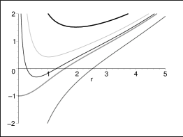
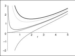
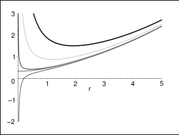
Figure 1: The plots of $f(r)$ for varying $M$ with a fixed $\beta Q$ ($\beta Q>1/2$ (left), $\beta Q=1/2$ (center), $\beta Q<1/2$ (right)) and a negative cosmological constant $\Lambda<0$ . We consider (top to bottom) $M=0,~{}0.95,~{}1.2,~{}M_{0},~{}1.5$ with $\beta=1$, $M_{0}\approx 1.236$ (left); $M=0,~{}0.85,~{}M_{0},~{}0.9,~{}1.2$ with $\beta=1/2$, $M_{0}\approx 0.874$ (center); and $M=0,~{}0.7,~{}M_{0},~{}0.75,~{}1.2$ with $\beta=1/3$, $M_{0}\approx 0.714$ (right), respectively for $Q=1,\Lambda=-1/5$.

Figure 2: The plots of the ADM mass $M$ vs. the wormhole radius $r_{0}$ (thick curves) and the black hole horizon radius $r_{+}$ (thin curves) for varying $\beta Q$ with a fixed cosmological constant $\Lambda<0$. The marginal mass $M_{0}$ is given by the mass value at $r_{0}$ or $r_{+}=0$. For wormholes, $M(r_{0})$ is a monotonically decreasing function with the maximum value $M_{0}$ at $r_{0}=0$. For black holes, $M(r_{+})$ is a monotonically increasing function with the minimum value $M_{0}$ at $r_{+}=0$ when $\beta Q\leq 1/2$ (three thin curves from below) and concave with the minimum $M^{*}<M_{0}$ at the extremal horizon $r_{+}^{*}$ when $\beta Q>1/2$ (top thin curve). We consider $\beta Q={2/3,~{}1/2,~{}2/4.5,~{}1/3}$ (top to bottom) with $\beta=2$ and $\Lambda=-1/5$.

In Fig.1 for the solution (7) one can easily see the existence of the throat $r_{0}$ satisfying the conditions (12) and (13), depending on the mass $M$ for given values of $\beta,Q,$ and ${\Lambda}$. Now, from the property of the metric function Garc:1984

$$\frac{d}{dr}(rf)=f+r\frac{df}{dr}=1-\Lambda r^{2}+2\beta^{2}r^{2}\left(1-\sqrt{1+\frac{Q^{2}}{\beta^{4}r^{4}}}\right),$$ (14)

one can find that at the throat $r_{0}$, the largest $r$ of $df/dr=0$,

$$f(r_{0})=1-\Lambda r_{0}^{2}+2\beta^{2}r_{0}^{2}\left(1-\sqrt{1+\frac{Q^{2}}{\beta^{2}r_{0}^{4}}}\right).$$ (15)

Comparing (15) with the general solution (7), the wormhole mass $M$ can be expressed in terms of $r_{0}$ as,

$$M(r_{0})=\frac{r_{0}^{3}}{3}\left[\Lambda-2\beta^{2}\left(1-\sqrt{1+\frac{Q^{2}}{\beta^{2}r_{0}^{4}}}\right)+\frac{2Q^{2}}{r_{0}^{4}}~{}{{}_{2}F}_{1}\left(\frac{1}{2},\frac{1}{4};\frac{5}{4};\frac{-Q^{2}}{\beta^{2}r_{0}^{4}}\right)\right],$$ (16)

which is a monotonically decreasing function of $r_{0}$ with the maximum value $M_{0}$ of (10) at $r_{0}=0$ (thick curves in Fig. 2). It is interesting to note that the mass of our new AdS wormhole without exotic matters can be negative for large $r_{0}$, similar to the conventional wormholes which require the exotic matters and violate energy conditions. This may be considered as another evidence that exotic matters cemented at the throat are not mandatory for constructing large scale wormholes.

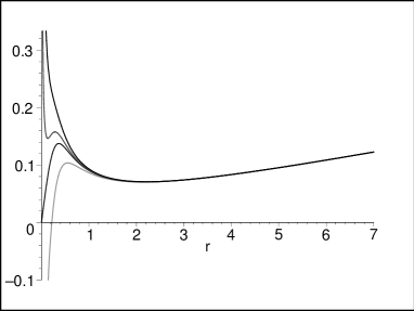
Figure 3: The plots of the Hawking temperature $T_{H}$ or $f(r_{0})/r_{0}$ vs. the black hole horizon radius $r_{+}$ or the wormhole throat radius $r_{0}$ for varying $\beta Q$ with a fixed cosmological constant $\Lambda<0$. We consider $\beta Q={2/3,~{}1/2,~{}2/4.5,~{}1/3}$ (bottom to top curves) with $\beta=2$, $\Lambda=-1/5$.

(16) is in contrast to the black hole mass $M$ in terms of the black hole horizon $r_{+}$, corresponding to the largest $r$ of $f(r)=0$,

$$M(r_{+})=\frac{r_{+}}{2}\left[1-\frac{\Lambda}{3}r_{+}^{2}+\frac{2}{3}\beta^{2}r_{+}^{2}\left(1-\sqrt{1+\frac{Q^{2}}{\beta^{2}r_{+}^{4}}}\right)+\frac{4}{3}\frac{Q^{2}}{r_{+}^{2}}~{}{{}_{2}F}_{1}\left(\frac{1}{2},\frac{1}{4};\frac{5}{4};\frac{-Q^{2}}{\beta^{2}r_{+}^{4}}\right)\right],$$ (17)

which is positive definite. This is a monotonically increasing function of $r_{+}$ with the minimum $M_{0}$ at $r_{+}=0$ when $\beta Q\leq 1/2$ so that there exists only the Schwarzschild-like (type I) black hole with one horizon (three thin curves from below in Fig. 2). On the other hand, when $\beta Q>1/2$ (top thin curve in Fig. 2), there exists the RN-like (type II) black hole with two horizons as well as the Schwarzschild-like black hole with one horizon. In this latter case, the black hole mass function (17) is concave with the minimum

$$M^{*}=\frac{r_{+}^{*}}{3}\left[1+\frac{2Q^{2}}{{r_{+}^{*}}^{2}}~{}{{}_{2}F}_{1}\left(\frac{1}{2},\frac{1}{4};\frac{5}{4};\frac{-Q^{2}}{\beta^{2}{r_{+}^{*}}^{4}}\right)\right],$$ (18)

which is smaller than $M_{0}$, at the “extremal” horizon $r_{+}^{*}$, where the outer horizon $r_{+}$ meets the inner horizon $r_{-}$ at

$$r^{*}_{+}=\sqrt{\frac{{\Lambda}-2\beta^{2}+2\sqrt{(\beta^{2}-{\Lambda}/2)^{2}+{\Lambda}({\Lambda}-4\beta^{2})(\beta^{2}Q^{2}-1/4)}}{{\Lambda}({\Lambda}-4\beta^{2})}}$$ (19)

with the vanishing Hawking temperature for the outer horizon $r_{+}$ (Fig.3),

$$T_{H} \equiv \frac{\hbar}{4\pi}\left.\frac{df}{dr}\right|_{r=r_{+}}{}$$ (20)

$$= \frac{\hbar}{4\pi}\left[\frac{1}{r_{+}}-{\Lambda}r_{+}+2\beta^{2}r_{+}\left(1-\sqrt{1+\frac{Q^{2}}{\beta r_{+}^{4}}}\right)\right].$$

In the latter case, the wormhole mass $M$ increases as the throat radius $r_{0}$ reduces, by accretion of ordinary (positive energy) matters until it reaches to the extremal black hole horizon $r_{+}^{*}$ where the wormhole mass is equal to the black hole mass $M(r_{0})=M(r_{+})=M^{*}$. Then, no further causal contact with the wormhole is possible “classically” afterwards since the throat is located inside the horizon $r_{+}$. Hence, for the case $\beta Q>1/2$, the ranges of $r_{0}$ and the wormhole mass $M(r_{0})$ are bounded by $r_{0}>r_{+}^{*},~{}M(r_{0})<M^{*}$ for the “observable” wormhole throat outside the black hole horizon $r_{+}$, in contrast to $r_{0}\geq 0,~{}M(r_{0})\leq M_{0}$ for the former case $\beta Q\leq 1/2$.

Finally we note that, near $r_{0}$, the metric function can be expanded as

$$f(r)=f(r_{0})+\frac{{\sigma}}{2}(r-r_{0})^{2}+{\cal O}[(r-r_{0})^{3}]$$ (21)

with the second moments,

$${\sigma}{\equiv}\left.\frac{d^{2}f}{dr^{2}}\right|_{r_{0}}=-2{\Lambda}+4\beta^{2}\left[1-\frac{1}{r_{0}^{4}}\left(1+\frac{Q^{2}}{\beta^{2}r_{0}^{4}}\right)^{-3/2}\right].$$ (22)

At large $r$, on the other hand, the metric function is expanded as

$$f(r)=1-\frac{\Lambda}{3}r^{2}-\frac{2M}{r}+\frac{Q^{2}}{r^{2}}-\frac{Q^{4}}{20\beta^{2}r^{6}}+{\cal O}(r^{-10}).$$ (23)

III Massive scalar perturbations in the new AdS-EBI wormhole

In this section, we consider the perturbations of a massive scalar field and its QNMs in the new AdS-EBI wormhole background. The wave equation for a minimally-coupled massive scalar field $\Phi(t,{\bf r})$ with mass $m$ is given by

$$\frac{1}{\sqrt{-g}}\partial_{\mu}\left(\sqrt{-g}g^{\mu\nu}\partial_{\nu}\Phi\right)-m^{2}\Phi=0.$$ (24)

Considering the mode solutions

$$\Phi(t,{\bf r})=e^{-i\omega t}Y(\theta,\phi)\frac{\widetilde{\varphi}(r)}{r},$$ (25)

with the spherical harmonics $Y(\theta,\phi)$ on ${\rm S}^{2}$, the wave equation reduces to the standard radial equation,

$$\left(\frac{d^{2}}{dr_{*}^{2}}+\omega^{2}\right)\widetilde{\varphi}(r)=\widetilde{V}(r)\widetilde{\varphi}(r),$$ (26)

where $r_{*}$ is the tortoise coordinate, defined by

$$dr_{*}\equiv\frac{dr}{f(r)},$$ (27)

and $\widetilde{V}(r)$ is the effective potential, given by

$$\widetilde{V}(r)=f(r)\left(\frac{l(l+1)}{r^{2}}+\frac{1}{r}\frac{df(r)}{dr}+m^{2}\right)$$ (28)

with the angular-momentum number $l$.

Choosing the tortoise coordinate $r_{*}=0$ at the throat $r_{0}$, one obtains

$$r_{*} \equiv \int^{r}_{r_{0}}f^{-1}(r)dr{}$$ (29)

$$= f^{-1}(r_{0})(r-r_{0})-\frac{{\sigma}}{3!}f^{-2}(r_{0})(r-r_{0})^{3}+{\cal O}[(r-r_{0})^{4}]$$

near the throat $r\approx r_{0}$ and

$$r_{*}=\int^{\infty}_{r_{0}}f^{-1}dr+\frac{3}{{\Lambda}r}+\frac{3}{{\Lambda}^{2}r^{3}}+{\cal O}(r^{-4})$$ (30)

at large $r$, using the asymptotic expansions (21) and (23), respectively. Here, $\int^{\infty}_{r_{0}}f^{-1}dr$ is the (finite) value of the tortoise coordinate $r_{*}(r)$ evaluated at $r=\infty$ and can be expanded as $-{3}{{\Lambda}^{-1}}(r_{0}^{-1}+{{\Lambda}^{-1}}r_{0}^{-3}+\cdots)$.

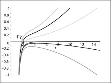
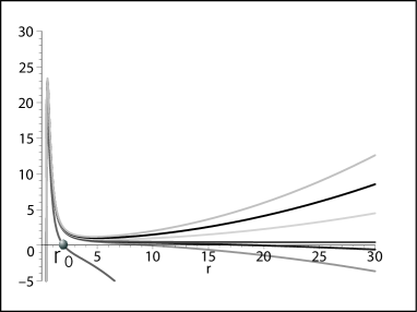
Figure 4: The plots of the effective potential $\widetilde{V}(r)$ for varying $m$ with a fixed $\beta Q>1/2$ and a cosmological constant ${\Lambda}<0$. We consider $m^{2}=-{\Lambda}/3,0,{\Lambda}/3,2{\Lambda}/3,3{\Lambda}/4,{\Lambda},-l(l+1)/r_{0}^{2}$ (top to bottom curves) for $l=0$ (left) and $l=2$ (right) with $M=10^{-5},{\Lambda}=-1/5,r_{0}\approx 1.96314$. $\widetilde{V}(r)$ vanishes at the throat $r_{0}$ only for the mass satisfying $m^{2}=-l(l+1)/r_{0}^{2}$; $m^{2}=0$ for $l=0$ (left, second curve from top) or a tachyonic mass $m^{2}=-6/r_{0}^{2}$ for $l=2$ (right, bottom curve).

From the near-throat behavior of the effective potential $\widetilde{V}$,

$$\widetilde{V}(r)=f(r_{0})\left(\frac{l(l+1)}{r_{0}^{2}}+m^{2}\right)+\frac{f^{2}(r_{0})}{r_{0}}\left(-\frac{2l(l+1)}{r_{0}^{2}}+{\sigma}\right)r_{*}+\cdots,$$ (31)

the mode solution near the throat is obtained as

$$\Phi(t,{\bf r})\approx A_{1}(\theta,\phi)\frac{e^{-i({\omega}t+kr_{*})}}{r}+A_{2}(\theta,\phi)\frac{e^{-i({\omega}t-kr_{*})}}{r}$$ (32)

with

$$k=\sqrt{{\omega}^{2}-\widetilde{V}(r_{0})},$$ (33)

where $\widetilde{V}(r_{0})=f(r_{0})[{l(l+1)}/{r_{0}^{2}}+m^{2}]$. Here, $A_{1}$ and $A_{2}$ parts represent purely ingoing and outgoing modes, respectively. Since QNMs are defined as solutions which are purely ingoing near the throat, we set $A_{2}(\theta,\phi)=0$ as our desired boundary condition at the throat. Here, it is interesting to note that the solutions at the throat are not light-like “generally” due to non-vanishing $f(r_{0})$ and the effective potential $\widetilde{V}(r_{0})$, in contrast to the always-light-like solutions at the black hole horizon $r_{+}$, where $f(r_{+})$ and the effective potential (28) vanish: The effective potential $\widetilde{V}(r_{0})$ may vanish when the mass of scalar field $m$ satisfies $m^{2}=-l(l+1)/r_{0}^{2}$ (for example, $m=0$ for $l=0$, or $m^{2}=-6/r_{0}^{2}$ for $l=2$), but generally it does not (Fig. 4).

On the other hand, at $r=\infty$, which corresponds to a finite value of $r_{*}|_{r=\infty}=\int^{\infty}_{r_{0}}f^{-1}dr$, the effective potential $\widetilde{V}(r)$ diverges as

$$\widetilde{V}(r)=-\frac{{\Lambda}}{3}r^{2}\left(m^{2}-\frac{2}{3}{\Lambda}\right)+\left(m^{2}-\frac{2}{3}{\Lambda}-\frac{{\Lambda}l(l+1)}{3}\right)+{{\cal O}(r^{-1})}.$$ (34)

In terms of the tortoise coordinate $r_{*}$, we have

$$\widetilde{V}(r) = -\frac{{\Lambda}}{3}\left(m^{2}-\frac{2}{3}{\Lambda}\right)\left(r_{*}-\int^{\infty}_{r_{0}}f^{-1}dr\right)^{-2}+\left[\frac{1}{3}\left(m^{2}-\frac{2}{3}{\Lambda}\right)-\frac{{\Lambda}l(l+1)}{3}\right]{}$$ (35)

$$+ {{\cal O}\left(r_{*}-\int^{\infty}_{r_{0}}f^{-1}dr\right)},$$

using $r=3{\Lambda}^{-1}\left(r_{*}-\int^{\infty}_{r_{0}}f^{-1}dr\right)^{-1}+\cdots$ for the limit $r\rightarrow\infty$, from (30). Then, the radial wave equation (26) reduces to

$$\left[\frac{d^{2}}{d\widetilde{r}_{*}^{2}}+\omega^{2}+\frac{{\Lambda}}{3}\left(l(l+1)-\frac{{\lambda}}{3}\right)+\frac{{\lambda}}{\widetilde{r}_{*}^{2}}\right]\widetilde{\varphi}(r)={{\cal O}(\widetilde{r}_{*})},$$ (36)

where ${\lambda}\equiv 3{\Lambda}^{-1}(m^{2}-2{\Lambda}/3)$ and $\widetilde{r}_{*}$ is the shifted tortoise coordinate $\widetilde{r}_{*}\equiv r_{*}-\int^{\infty}_{r_{0}}f^{-1}dr$, which approaches zero as $r\rightarrow\infty$.

Now, near $\widetilde{r}_{*}=0$ ($r=\infty$), the leading order solution of (36) is obtained as

$$\widetilde{\varphi}(r)\approx B_{1}\widetilde{r}_{*}^{\frac{1}{2}(1+\sqrt{1-4{\lambda}})}+B_{2}\widetilde{r}_{*}^{\frac{1}{2}(1-\sqrt{1-4{\lambda}})}.$$ (37)

Since the norm of the wave function $\Phi$ is given by

$$\int dx^{3}\Phi^{*}\Phi\sim\int^{\infty}_{r_{0}}dr\widetilde{\varphi}^{*}\widetilde{\varphi}\sim\int^{0}_{-\delta}\frac{d\widetilde{r}_{*}}{\widetilde{r}_{*}^{2}}\widetilde{\varphi}^{*}\widetilde{\varphi},$$ (38)

where ${\delta}\equiv\int^{\infty}_{r_{0}}f^{-1}dr~{}(<\infty)$, the solution (37) is square-integrable only for $B_{2}=0$ and

$${\lambda}<\frac{1}{4},$$ (39)

or equivalently

$$m^{2}>\frac{3{\Lambda}}{4}.$$ (40)

This result agrees also with the condition of regularity or finite energy of the solution Calo:1969 ; Brei:1982 . In particular, (40) represents the stability condition of massive scalar perturbations in the global AdS space , $m^{2}>m^{2}_{\rm{BF}}$ with the BF bound $m^{2}_{\rm{BF}}=3{\Lambda}/4$ Brei:1982 ; Moro:2010 . Moreover, note that the solution (37) with the bound (40), satisfies the vanishing Dirichlet boundary condition at $r=\infty$ ($\widetilde{r}_{*}=0$) even though the effective potential $\widetilde{V}$ is not positive infinite (Fig. 4): At $r=\infty$, $\widetilde{V}$ is positive infinite for $m^{2}>2{\Lambda}/3$ but zero or negative infinite for $2{\Lambda}/3\geq m^{2}>3{\Lambda}/4$. The usual stability criterion based on the positivity of the effective potential is not quite correct when considering massive perturbations in AdS background for the latter mass range Chan:1985 .

IV Massive  Quasi-Normal Modes

QNMs are defined as the solutions which are purely ingoing near the throat $\Phi\sim e^{-i({\omega}t+kr_{*})}$. In this paper, our interest is the dependence of QNMs on the mass of perturbed fields and in this section we will consider their computations, which are called “massive” QNMs Ohas:2004 , based on the approach of Horowitz and Hubeny (HH) Horo:1999 . In order to study QNMs, it is convenient to work with the Eddington-Finkelstein coordinate by introducing the ingoing null coordinate $v=t+r_{*}$ with the metric

$$ds^{2}=-f(r)dv^{2}+2dvdr+r^{2}(d\theta^{2}+\sin^{2}\theta d\phi^{2}).$$ (41)

Considering the mode solution,

$$\Phi(t,{\bf r})=e^{-i\omega v}Y(\theta,\phi)\frac{\varphi(r)}{r},$$ (42)

the wave equation (24) reduces to the radial equation for $\varphi(r)$,

$$f(r)\frac{d^{2}\varphi(r)}{dr^{2}}+\left(\frac{df(r)}{dr}-2i\omega\right)\frac{d\varphi(r)}{dr}-V(r)\varphi(r)=0$$ (43)

with the reduced effective potential $V(r)$,

$$V(r)=\frac{l(l+1)}{r^{2}}+\frac{1}{r}\frac{df(r)}{dr}+m^{2}.$$ (44)

Note that, as in the effective potential $\widetilde{V}(r)$, the reduced potential $V(r)$ is not positive definite and its positivity depends on $m^{2}$ (Fig. 5): $V(r)$ is positive definite for the whole region of $r\geq r_{0}$ only for $m^{2}>2{\Lambda}/3$.

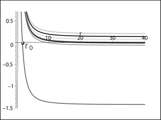
Figure 5: The plots of the reduced effective potential ${V}(r)$ for the corresponding effective potential $\widetilde{V}(r)$ in Fig. 4.

To compute QNMs, we will expand the solution as a power series around the wormhole throat $r_{0}$ and impose the vanishing Dirichlet boundary conditions at $r=\infty$, following the approach of HH Horo:1999 . In order to treat the whole region of interest, $r_{0}\leq r<\infty$, into a finite region, we introduce a new variable $x=1/r$ so that the metric (41) becomes

$$ds^{2}=-f(x)dv^{2}+\frac{1}{x^{2}}(-2dvdx+d\theta^{2}+\sin^{2}\theta d\phi^{2}).$$ (45)

The scalar field equation can be written as

$$s(x)\frac{d^{2}\varphi(x)}{dx^{2}}+\frac{t(x)}{x-x_{0}}\frac{d\varphi(x)}{dx}+\frac{u(x)}{(x-x_{0})^{2}}\varphi(x)=0,$$ (46)

where $x_{0}=1/r_{0}$ and the coefficient functions are given by

$$s(x) = -\frac{x^{4}f(x)}{x-x_{0}},{}$$

$$t(x) = -2x^{3}f(x)-x^{4}\dot{f}(x)-2i{\omega}x^{2},{}$$

$$u(x) = (x-x_{0})\left[l(l+1)x^{2}-x^{3}\dot{f}(x)+m^{2}\right].$$ (47)

The overdot ($\dot{~{}}$) represents the derivative with respects to $x$. Since $f(x_{0})>0$ in our wormhole system, one can remove the overall $(x-x_{0})^{-1}$ factor in (46) so that $x=x_{0}$ is not a singular point, whereas there is one regular singular point at the spatial infinity $x=0$. Then one can expand equation (46) around the throat $x_{0}$ up to the pole at $x=0$ and solve the equation at each order of the expansion.

First, expanding $s,t,u$ around $x=x_{0}$ as

$$s(x) = \sum_{n=-1}^{\infty}s_{n}(x-x_{0})^{n},{}$$

$$t(x) = \sum_{n=0}^{\infty}t_{n}(x-x_{0})^{n},{}$$

$$u(x) = \sum_{n=0}^{\infty}u_{n}(x-x_{0})^{n},$$ (48)

one can obtain the first few coefficients of them as follows,

$$s_{-1}=-x_{0}^{4}f(x_{0}),~{}s_{0}=-4x_{0}^{3}f(x_{0}),~{}s_{1}=-6x_{0}^{2}f(x_{0})-\frac{1}{2}x_{0}^{4}\ddot{f}(x_{0}),{}$$

$$t_{0}=-2x_{0}^{2}\left[x_{0}f(x_{0})+i{\omega}\right],~{}t_{1}=-x_{0}\left[6x_{0}f(x_{0})+x_{0}^{3}\ddot{f}(x_{0})+4i{\omega}\right],{}$$

$$t_{2}=-2i{\omega}+~{}{({\rm non-}{\omega}~{}{\rm terms})}~{},~{}t_{n(>2)}=~{}{({\rm non-}{\omega}~{}{\rm terms})}~{},{}$$

$$u_{0}=0,~{}u_{1}=l(l+1)x_{0}^{2}+m^{2},~{}u_{2}=x_{0}\left[2l(l+1)-x_{0}^{2}\ddot{f}(x_{0})\right],$$ (49)

where we have used $\dot{f}(x_{0})=0$ and

$$\ddot{f}(x_{0})=x_{0}^{-4}\left.\frac{d^{2}f}{dr^{2}}\right|_{r_{0}}={\sigma}x_{0}^{-4}$$ (50)

with the second moments ${\sigma}=(d^{2}f/dr^{2})|_{r_{0}}$ given by (22) .

Now in order to consider the expansion of the solution around the throat $r_{0}$, we first set $\varphi=(x-x_{0})^{{\alpha}}$ as the lowest order solutions. Then, at the leading order $n=-1$, one obtains the indicial equation,

$$s_{-1}{\alpha}({\alpha}-1)=-x_{0}^{4}f(x_{0}){\alpha}({\alpha}-1)=0,$$ (51)

which gives two solutions, ${\alpha}=0$ and ${\alpha}=1$. The first solution, ${\alpha}=0$, corresponds to the ingoing mode $\Phi\sim e^{-i{\omega}v}$ near the throat. The second solution, ${\alpha}=1$, is also an ingoing mode near the throat but vanishing at the throat as $\Phi\sim e^{-i{\omega}v}(x-x_{0})$. Since in this paper we want to consider non-vanishing ingoing modes to study QNMs, we take only the ${\alpha}=0$ case . Then the desired solution can be expanded as

$$\varphi(x)=\sum_{n=0}^{\infty}a_{n}(x-x_{0})^{n}.$$ (52)

Plugging (52) into (46) with the expansion (48), one obtains the recursion relation for $a_{n}~{}(n\neq 0,1)$ as follows:

$$a_{n}=-\frac{1}{P_{n}}\sum_{k=0}^{n-1}\left[k(k-1)s_{n-k-1}+kt_{n-k-1}+u_{n-k-1}\right]a_{k},$$ (53)

where

$$P_{n}=n(n-1)s_{-1}=-n(n-1)x_{0}^{4}f(x_{0}).$$ (54)

Generally we can get two parameter families of solutions in terms of $a_{0}$ and $a_{1}$ near $x=x_{0}$. As we have discussed already, $a_{0}$ term corresponds to a pure ingoing mode at $x=x_{0}$ so that $a_{0}$ should be kept and in this paper we set $a_{0}=1$ for convenience. On the other hand, $a_{1}$ term corresponds to a vanishing ingoing mode at $x=x_{0}$ so that we may discard this family of solution, which actually satisfies the additional Neumann boundary condition for $\varphi$, i.e., $\varphi^{\prime}|_{x_{0}}=a_{1}\equiv 0$. In this paper, we are only interested in this case for simplicity.

As $r\rightarrow\infty$, (46) reduces to

$$r^{2}\frac{d^{2}\varphi(r)}{dr^{2}}+2r\frac{d\varphi(r)}{dr}-\left(2-\frac{3m^{2}}{{\Lambda}}\right)\varphi(r)\approx 0,$$ (55)

which leads to the asymptotic solution as

$$\varphi(r)\approx C_{1}r^{-\frac{1}{2}(1+\sqrt{9-12m^{2}/{\Lambda}})}+C_{2}r^{-\frac{1}{2}(1-\sqrt{9-12m^{2}/{\Lambda}})},$$ (56)

corresponding to the solution in (37). Since we are interested in the normalizable modes, we take $C_{2}=0$ and the desired solution is $\varphi(r)\sim r^{-\frac{1}{2}(1+\sqrt{9-12m^{2}/{\Lambda}})}$, which also satisfies the vanishing Dirichlet boundary condition $\varphi(r)\rightarrow 0$ as $r\rightarrow\infty$ ($x\rightarrow 0$). This means that we impose the boundary condition as an algebraic equation at $x=0$,

$$\varphi(0)=\sum_{n=0}^{\infty}a_{n}(-x_{0})^{n}=0,$$ (57)

which is satisfied only for some discrete values of ${\omega}$ since $a_{n}$’s are functions of ${\omega}$ from (53). If the sum (57) is convergent, one can truncate the summation at some large order $n=N$ where the partial sum beyond $n=N$ does not change within the desired precision. Because this approach can easily be implemented numerically, particularly in Mathematica, the coefficients $a_{n},s_{n},t_{n},u_{n}$ can be computed up to an arbitrary order $N$. In the next section, we present the numerical computation of QNM frequencies ${\omega}\equiv{\omega}_{R}-i{\omega}_{I}$ based on this method.

V Numerical Results and Their Interpretations

In this section, we will show the results of numerical computation of QNMs as described in the previous section. In this paper, we consider only the “lowest” QNMs, whose absolute magnitude, $|{\omega}|=\sqrt{{\omega}_{R}^{2}+{\omega}_{I}^{2}}$, is the smallest, unless stated otherwise. First of all, Fig. 6 and 7 show the lowest QNM frequency ${\omega}={\omega}_{R}-i{\omega}_{I}$ as a function of $m^{2}$ for varying $M$ and $Q$. Here, we focus on the case of $\beta Q>1/2$, where the well-defined GR limit of $\beta\rightarrow\infty$ exists JKim:2016 . The result shows that the perturbations are stable (${\omega}_{I}>0$) if $m^{2}$ is above certain threshold values $m_{*}^{2}$ ($-0.16769,-0.16720,-0.16704$ for $M=10^{-5},0.1,0.15$ with $Q=1$ (Fig. 6); $-0.16769,-0.16728,-0.16704$ for $Q=1,0.9,0.85$ with $M=10^{-5}$ (Fig. 7)). For a given value of $M$ or $Q$, QNM frequencies ${\omega}_{I}$ and ${\omega}_{R}$ increase as $m^{2}$ increases above $m_{*}^{2}$. Here, we note that the critical mass $m_{*}^{2}$ is close to the BF bound of (40), $m^{2}_{\rm{BF}}=-3{\Lambda}/4=-0.15$ Brei:1982 . On the other hand, for a given value of $m^{2}$, ${\omega}_{I}$ and ${\omega}_{R}$ increase as $M$ decreases or $Q$ increases, corresponding to increasing throat radius $r_{0}$ from (16) (Fig. 2). Neglecting the small differences of $m_{*}^{2}$ for different $M$ and $Q$, we may approximately fit the numerical result of the $m^{2}$ dependence in Fig. 6 and 7 to the analytic functions

$${\omega}_{I}\approx b_{1}(m^{2}-m_{*}^{2})+b_{2}(m^{2}-m_{*}^{2})^{2}+\cdots,{}$$

$${\omega}_{R}\approx\frac{1}{2}+c_{1}(m^{2}-m_{*}^{2})+c_{2}(m^{2}-m_{*}^{2})^{2}+\cdots,$$ (58)

near the critical mass squared $m_{*}^{2}$, with the approprite coefficients, $b_{n}$ and $c_{n}(n=1,2,\cdots).$

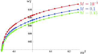
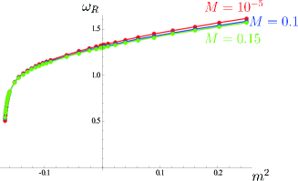
Figure 6: The plots of ${\omega}={\omega}_{R}-i{\omega}_{I}$ vs. $m^{2}$ for varying $M$ with a fixed $\beta Q>1/2$ and ${\Lambda}<0$. Here, we consider $l=2,\beta=1,Q=1,{{\Lambda}=-0.2}$, and $M=10^{-5},{0.1,0.15}$ (top to bottom curves). The result shows the instability (${\omega}_{I}<0$) of massive perturbations below certain (threshold) values of mass squared, $m^{2}<m_{*}^{2}$ with $m_{*}^{2}\approx{-0.16769,-0.16720,-0.16704}$, respectively.

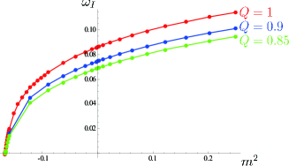
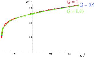
Figure 7: The plots of ${\omega}={\omega}_{R}-i{\omega}_{I}$ vs. $m^{2}$ for varying $Q$ with a fixed $\beta Q>1/2$ and ${\Lambda}<0$. Here, we consider $l=2,\beta=1,{{\Lambda}=-0.2},M=10^{-5}$, and $Q=1,0.9,0.85$ (top to bottom). The result shows nearly the same on-set point of instability as in Fig. 6, $m^{2}_{*}\approx-0.16769,-0.16728,-0.16704$, respectively.

Fig. 8 shows the QNM frequency as a function of $m^{2}$ for varying negative cosmological constant ${\Lambda}$ with fixed $M$ and $Q$. The result shows that the critical mass squared shifts as $m_{*}^{2}\approx-0.16769,-0.11156,-0.08294$ for ${\Lambda}=-0.2,-0.13,-0.1$, respectively. This is consistent with the shifts of the corresponding $BF$ bounds, $m_{\rm{BF}}^{2}=3{\Lambda}/4=-0.15,-0.1,-0.075$.

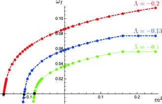
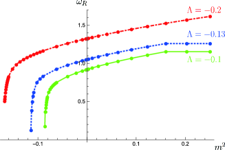
Figure 8: The plots of ${\omega}={\omega}_{R}-i{\omega}_{I}$ vs. $m^{2}$ for varying ${\Lambda}<0$ with a fixed $\beta Q>1/2$. Here, we consider $l=2,\beta=1,M=10^{-5},Q=1$, and ${\Lambda}=-0.2,-0.13,-0.1$ (top to bottom). The result shows the shifts of on-set points of instability as $m_{*}^{2}\approx-0.16769,-0.11156,-0.08294$ for ${\Lambda}=-0.2,-0.13,-0.1$, respectively.

Fig. 9 shows the lowest QNM frequency as a function of $m^{2}$ for varying angular-momentum number $l$. The result shows that the critical mass shifts as $m_{*}^{2}\approx-0.16769,-0.16679,-0.15524$ for $l=2,1,0$, respectively. Especially for $l=0$, it shows a level crossing between the lowest pure-imaginary mode representing an over-damping (purple color) and the lowest complex mode (pink color) at $m^{2}\approx-0.1089$ before the critical mass $m^{2}_{*}$ is being reached, so that the instability is governed by the used-to-be higher (pure) imaginary frequency modes . On the other hand, there are discontinuities in ${\omega}_{I}$ and ${\omega}_{R}$ at $m^{2}\approx-0.0784$ for the lowest complex frequency ${\omega}={\omega}_{R}-i{\omega}_{I}$ (green color) even before the level-crossing point .

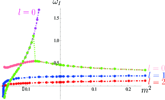
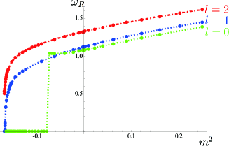
Figure 9: The plots of ${\omega}={\omega}_{R}-i{\omega}_{I}$ vs. $m^{2}$ for varying $l$ (for left, $l=0$ (top two curves), $l=1$ (second from bottom), $l=2$ (bottom); for right, $l=0,1,2$ (bottom to top)) with a fixed $\beta Q>1/2$ and all other parameters. Here, we consider $\beta=1,Q=1,M=10^{-5},{\Lambda}=-0.2$. The result shows that the critical mass shifts as $m_{*}^{2}\approx-0.16769,-0.16679,-0.15524$ for $l=2,1,0$, respectively. When $l=0$, it shows a level crossing between the lowest pure-imaginary mode (purple color) and the lowest complex mode (pink color) at $m^{2}\approx-0.1089$ before the on-set of instability is being reached. Moreover, there are discontinuities in ${\omega}_{I}$ and ${\omega}_{R}$ for the lowest ${\omega}={\omega}_{R}-i{\omega}_{I}$ (green color) at $m^{2}\approx-0.0784$ before the level-crossing point.

Fig. 10 shows the QNM frequency as a function of $l$ for varying $m^{2}$. For small $l$ ($l\leq 5$), ${\omega}_{I}$ decreases but ${\omega}_{R}$ increases (except for the case $m^{2}<0$) as $l$ increases, whereas for large $l$, both ${\omega}_{I}$ and ${\omega}_{R}$ increase as $l$ increases. It is interesting to note that there is a bouncing point of ${\omega}_{I}$, where ${\omega}_{I}=0$ at $l=5$. Here we have considered only the case $m^{2}>m_{*}^{2}$, which is stable for small $l$.

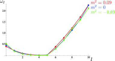
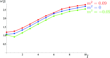
Figure 10: The plots of ${\omega}={\omega}_{R}-i{\omega}_{I}$ vs. $l$ for varying $m^{2}$ ($m^{2}=0.09,0,-0.09$ (top to bottom)) with a fixed $\beta Q>1/2$ and all other parameters. Here, we consider $\beta=1,Q=1,M=10^{-5},{\Lambda}=-0.2$. For small $l~{}(\leq 5)$, ${\omega}_{I}$ decreases as $l$ increases but ${\omega}_{R}$ increases (except for the case $m^{2}<0$), whereas for large $l$ both ${\omega}_{R}$ and ${\omega}_{I}$ increase as $l$ increases. There exists a bouncing point of ${\omega}_{I}$, where ${\omega}_{I}=0$ at $l=5$. Here we consider only the case $m^{2}>m_{*}^{2}$, which is stable for small $l$.

Fig. 11 shows the QNM frequency as a function of $r_{0}$ for varying $m^{2}$ in Fig. 6. Though the result is preliminary since there are only limited data points, i.e., for a given value of $m$, only three points of $r_{0}$ which correspond to the three values of $M$ in Fig. 6, the result indicates interestingly the linear dependence of QNM frequency to the throat radius. Explicitly, the curves can be fitted to

$${\omega}_{I}\approx d_{0}+d_{1}r_{0},~{}~{}{\omega}_{R}\approx e_{0}+e_{1}r_{0}$$ (59)

with $d_{0}=-0.15050,-0.14728,-0.13157,~{}d_{1}=0.12718,0.11894,0.10046,~{}e_{0}=0.98624,0.96175,0.92391,~{}e_{1}=0.23483,0.18614,0.12275$ for $m^{2}\approx 0.09,0,-0.09$, respectively. This is similar to the case for large black holes where QNM frequency depends linearly on the horizon radius (${\omega}_{I},{\omega}_{R}\propto r_{+}$) Horo:1999 ; Wang:2000 .

The asymptotic linear dependence can also be understood as the result of the scaling behavior Horo:1999 ; Greg:1993 ; Yin:2010 ,

$$r\rightarrow\alpha r,~{}t\rightarrow\alpha t,~{}\omega\rightarrow\omega/\alpha,~{}\beta\rightarrow\beta/\alpha,{}$$

$$m\rightarrow m/\alpha,~{}M\rightarrow\alpha M,~{}Q\rightarrow\alpha Q,~{}\Lambda\rightarrow\Lambda/\alpha^{2},$$ (60)

by which the perturbation equation (46) is unchanged. This means that the QNM frequency ${\omega}={\omega}_{R}-i{\omega}_{I}$, which is a function of $r_{0},{\Lambda},Q,\beta$, and $m$, should have the following form

$${\omega}\sim{\Lambda}r_{0}+\frac{1}{r_{0}}+\beta+\frac{Q^{2}}{r_{0}^{3}}+\frac{Q^{2}}{\beta^{2}r_{0}^{5}}+r_{0}m^{2}+\frac{r_{0}}{{\Lambda}}m^{4}+\cdots$$ (61)

in order to have the scaling $\omega\rightarrow\omega/\alpha$. For large $r_{0}$, the dominant terms are given by

$${\omega}\approx\bar{\zeta}{\Lambda}r_{0}+\bar{\eta}\beta+\left(\bar{\delta}m^{2}+\bar{\gamma}{\Lambda}^{-1}m^{4}+\cdots\right)r_{0},$$ (62)

where $\bar{\zeta},\bar{\eta},\bar{\delta}$, and $\bar{\gamma}$ are scale invariant coefficients, which agrees with the behavior of (59) .

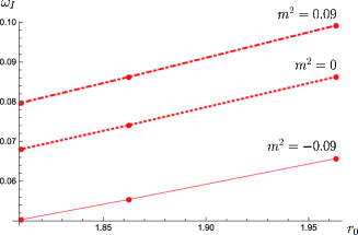
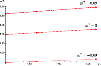
Figure 11: The plots of ${\omega}={\omega}_{R}-i{\omega}_{I}$ vs. $r_{0}$ for varying $m^{2}$ ($0.09,0,-0.09$ (top to bottom)) with a fixed $\beta Q>1/2$ and all other parameters. Here, we consider three values of $r_{0}$ which correspond to the three curves with $M=10^{-5},0.1,0.15\times 10^{-1}$ in Fig. 6. The result shows the linear dependence of ${\omega}_{I},{\omega}_{R}$ on $r_{0}$.

So far, we have studied the case $\beta Q>1/2$, which has a well-defined GR limit at $\beta\rightarrow\infty$. Now, we show in Fig. 12 the case $\beta Q\leq 1/2$, which do not have a GR limit. The result shows that there is no oscillatory part (${\omega}_{R}=0$) and moreover the critical mass squared $m_{*}^{2}<0$ does not occur in this case. Rather, it shows another critical mass squared $m_{c}^{2}\approx 1.0326$ for $\beta Q<1/2$ so that the perturbations would be completely “frozen”, i.e., ${\omega}={\omega}_{R}-i{\omega}_{I}=0$, for $m^{2}>m_{c}^{2}$. Even though this result could be preliminary too since we may not neglect the back reaction of the wormhole geometry for the heavy-mass perturbations Kono:2004 , it seems to agree with the so-called “quasi-resonance modes (QRMs)” with ${\omega}_{I}=0$ in massive QNMs, though the oscillatory parts are different, i.e., ${\omega}_{R}=0$ in our wormhole case but ${\omega}_{R}\neq 0$ in QRMs Ohas:2004 .

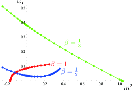
Figure 12: The plots of ${\omega}={\omega}_{R}-i{\omega}_{I}$ vs. $m^{2}$ for varying $\beta$ with a fixed $Q$ and all other parameters. Here, we consider $l=2,Q=1,M=10^{-5},{\Lambda}=-0.2$. The on-set of instability for $m^{2}<0$ occurs only for $\beta Q>1/2$ which was considered in Fig. 6 and 7. For $\beta Q<1/2$, it shows another on-set of instability at $m^{2}\approx 1.03326$. Moreover, for $\beta Q\leq 1/2$, the result shows only the pure-imaginary modes (${\omega}_{R}=0$). For $\beta Q>1/2$, ${\omega}_{R}$ was shown in Fig. 6.

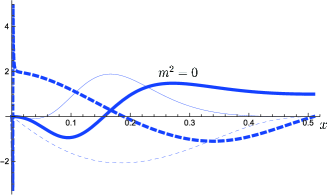
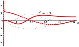
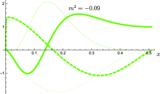
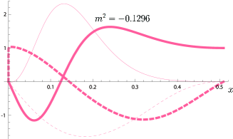
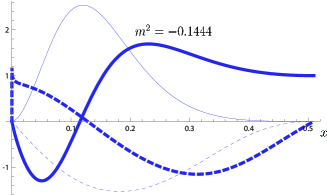
Figure 13: The plots of the numerically reconstructed (truncated) wave function $\varphi_{N}$ vs. $x$ for varying $m^{2}$ ($0,0.09,-0.09,-0.1296,-0.1444$ (blue, red, green, pink, purple)) and $M=10^{-5}$ in Fig. 6. The thick and thin solid lines denote $\mbox{Re}(\varphi_{N})$ and $\mbox{Im}(\varphi_{N})$, respectively and one can confirm that these satisfy the vanishing Dirichlet boundary condition ($\varphi(x)\rightarrow 0$) as $x\rightarrow 0$ and the vanishing Neumann boundary condition ($d\varphi/dx\rightarrow 0)$ as $x\rightarrow x_{0}\approx 0.50939$. The dotted lines denote their asymptotic exponents, $x\ln\mbox{Re}(d\varphi_{N}/dx),~{}x\ln\mbox{Im}(d\varphi_{N}(x)/dx)$ and these correctly approach the exponent of our asymptotic solution $\varphi(x)\sim x^{\frac{1}{2}(1+\sqrt{9-12m^{2}/{\Lambda}})}$ in (56), which are computed as $2,2.39737,1.44868,1.05317,0.78983$ for $m^{2}=0,0.09,-0.09,-0.1296,-0.1444$, respectively.

Before finishing this section, we end up with some remarks about the consistency of our numerical results. First, Fig. 13 shows the truncated wave function $\varphi_{N}(x)$, reconstructed from the numerically obtained $a_{n}$’s in (52) up to the order $N=300$. These show the vanishing Dirichlet boundary condition ($\varphi(x)\rightarrow 0)$ as $x\rightarrow 0$ and the vanishing Neumann boundary condition ($d\varphi/dx\rightarrow 0$) as $x\rightarrow x_{0}$ from our choice of $\alpha=1$ in the indicial equation (51). Moreover, the asymptotic behavior of our desired wave function $\varphi(x)\sim x^{\frac{1}{2}(1+\sqrt{9-12m^{2}/{\Lambda}})}$ in (56), whose exponent can be captured by $x\ln(d\varphi/dx)\rightarrow\frac{1}{2}(1+\sqrt{9-12m^{2}/{\Lambda}})$ as $x\rightarrow 0$, which are computed as $2,2.39737,1.44868,1.05317,0.78983$ for $m^{2}=0,0.09,-0.09,-0.1296,-0.1444$, is well confirmed by the numerically reconstructed wave function .

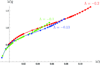
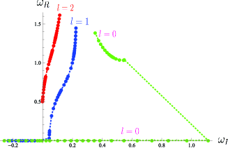
Figure 14: The plots of ${\omega}_{R}$ vs. ${\omega}_{I}$ for the results in Fig. 8 with varying ${\Lambda}<0$ $(l=2)$ (left), and in Fig. 9 with varying $l$ $({\Lambda}=-0.2)$ (right). The left shows a smooth non-vanishing function ${\omega}_{R}={\omega}_{R}({\omega}_{I})$ across the instability point for ${\Lambda}=-0.13$ (blue) and ${\Lambda}=-0.1$ (green). The right shows the vanishing ${\omega}_{R}$ for the unstable region (${\omega}_{I}<0$) with non-smooth transitions before the instability point for $l=1$ (blue) and $l=0$ (green). The red curve is the case ${\Lambda}=-0.2$ ($l=2$) in Fig. 8 and Fig. 9 shows also the smooth ${\omega}_{R}={\omega}_{R}({\omega}_{I})$ across the instability point though it is not quite clear in the plot.

Second, for the unstable modes (${\omega}_{I}<0$) beyond the critical mass $m^{2}<m^{2}_{*}$, Fig. 8 and 9 show that there exits the oscillation mode with the non-vanishing ${\omega}_{R}$ which is continuously changing across the on-set point of the instability (${\Lambda}=-0.13,-0.1$ case $(l=2)$ in Fig. 8 and $l=1$ case (${\Lambda}=-0.2$) in Fig. 9). But for some cases ${\omega}_{R}$ vanishes with a sudden discontinuity before the on-set point of instability is being reached ($l=0$ case (${\Lambda}=-0.2$) in Fig. 9). This seems to contradict the argument in the literature which claims that “ ${\omega}_{R}=0$ for the unstable mode, ${\omega}_{I}<0$ ”, though there is no restriction on ${\omega}_{R}$ for the stable mode, ${\omega}_{I}>0$ Kono:2008 ; Moon:2011 . In order to clarify this issue, we consider the integral,

$$I=\int^{{\delta}}_{0}\left[\widetilde{\varphi}^{*}\frac{d^{2}\widetilde{\varphi}}{dr^{2}_{*}}+({\omega}^{2}-\widetilde{V})|\widetilde{\varphi}|^{2}\right]dr_{*}{=0}$$ (63)

from the throat ($r_{*}=0$) to spatial infinity ($r_{*}={\delta}$), after multiplying the complex conjugated function $\widetilde{\varphi}^{*}$ by (26). The partial integration of the first gives

$$I=\left.\widetilde{\varphi}^{*}\frac{d\widetilde{\varphi}}{dr_{*}}\right|^{{\delta}}_{0}+\int^{{\delta}}_{0}\left[-\left|\frac{d\widetilde{\varphi}}{dr_{*}}\right|^{2}+({\omega}^{2}-\widetilde{V})|\widetilde{\varphi}|^{2}\right]dr_{*}=0.$$ (64)

Considering the desired wave function $\widetilde{\varphi}(x)\sim\widetilde{r}_{*}^{\frac{1}{2}(1+\sqrt{1-4{\lambda}})}$ with $B_{2}=0$ in (37), the boundary term at infinity $r_{*}={\delta}>0$ (or $\widetilde{r}_{*}=0$) vanishes and one finds the imaginary part of the integral

$${\rm Im}(I)=-{\rm Im}\left(\left.\widetilde{\varphi}^{*}\frac{d\widetilde{\varphi}}{dr_{*}}\right|_{r_{*}=0}\right)-2{\omega}_{R}{\omega}_{I}\int^{{\delta}}_{0}|\widetilde{\varphi}|^{2}dr_{*}=0.$$ (65)

When considering only the ingoing solution $\widetilde{\varphi}\sim e^{-ikr_{*}}$ with $A_{2}=0$ in (32), we now have

$${\rm Im}(I)=k_{R}\left|\widetilde{\varphi}(r_{*}=0)\right|^{2}-2{\omega}_{R}{\omega}_{I}\int^{{\delta}}_{0}|\widetilde{\varphi}|^{2}dr_{*}=0,$$ (66)

from $({d\widetilde{\varphi}}/{dr_{*}})|_{r_{*}=0}=-ik\widetilde{\varphi}|_{r_{*}=0}$ with $k=\sqrt{{\omega}^{2}-\widetilde{V}(r_{0})}$ in (33). On the other hand, when allowing an additional homogeneous solution in (32), $\widetilde{\varphi}\sim e^{-ikr_{*}}+i(k-{\omega})r_{*}$, we have

$${\rm Im}(I)={\omega}_{R}\left[\left|\widetilde{\varphi}(r_{*}=0)\right|^{2}-2{\omega}_{I}\int^{{\delta}}_{0}|\widetilde{\varphi}|^{2}dr_{*}\right]=0,$$ (67)

from $({d\widetilde{\varphi}}/{dr_{*}})|_{r_{*}=0}=-i{\omega}\widetilde{\varphi}|_{r_{*}=0}$ as if the solution is light-like at the throat, similar to the case for the black hole Kono:2008 ; Moon:2011 . Actually, this second case corresponds to our choice of vanishing Neumann boundary condition $({d\varphi}/{dr_{*}}|_{r_{*}=0}=0)$ from the solution $\varphi={e^{i{\omega}r_{*}}\widetilde{\varphi}}\sim e^{i({\omega}-k)r_{*}}+i(k-{\omega}){r_{*}}e^{i{\omega}r_{*}}$. Now, for the simplicity of our discussion, let us consider only the second case , which we have studied numerically in this paper. From (67), one finds naively that “ non-vanishing ${\omega}_{R}$ may imply ${\omega}_{I}>0$, i.e., stable modes ” Kono:2008 ; Moon:2011 . However, here it is important to note that this is the only case when ${\omega}_{R}$ (or $k_{R}$) is “independent” on ${\omega}_{I}$: When ${\omega}_{R}$ (or $k_{R}$) is not independent on ${\omega}_{I}$, the solution ${\omega}_{I}>0$ may not be the unique possibility, generally. For example, if we consider ${\omega}_{R}$ as a function of ${\omega}_{I}$, ${\omega}_{R}={\omega}_{R}({\omega}_{I})$, (67) is generally a non-linear equation for one independent variable ${\omega}_{I}$ and its solution needs not to agree with the previous naive one without separating independent variables, which may lead to misleading solutions. This means that ${\omega}_{R}\neq 0,~{}{\omega}_{I}<0$ (oscillating, unstable modes) can also be the possible solution depending on the details of ${\omega}_{R}={\omega}_{R}({\omega}_{I})$. Actually, Fig. 14 shows the relation ${\omega}_{R}\approx 1/2+a~{}{\omega}_{I}+b~{}{\omega}_{I}^{2}\cdots$ which allows the continuous solution of ${\omega}_{R}\neq 0,{\omega}_{I}<0$, as implied by the result of (58) (left), as well as the usual discontinuous solution (right, $l=0,1$ case). This indicates the existence of more fundamental reason for the relation . The usual result ${\omega}_{R}=0,{\omega}_{I}<0$ for the case $l=0$ may be due to the independence of ${\omega}_{I}(<0)$ from ${\omega}_{R}$ after the level crossing of two initially different modes.

Finally, in order to obtain reliable numerical results we need to compute the partial sum with the typical truncation of the order of $N=250$ (Fig. 15). In this work, we consider up to $N=300$ for most computations, but we consider up to $N=400$ for the level crossing of $l=0$ QNMs in Fig. 9.

VI Concluding Remarks

We have studied QNMs for a massive scalar field in the background of a natural AdS wormhole in EBI gravity, which has been recently constructed without exotic matters. For the case where the GR limit exists, i.e., $\beta Q>1/2$, we have shown numerically the existence of a BF-like bound $m_{*}^{2}<0$ so that the perturbation is unstable for a tachyonic mass $m^{2}<m_{*}^{2}$, like the perturbation in the global AdS. Furthermore, we have shown that the unstable modes (${\omega}_{I}<0$) can also have oscillatory parts (${\omega}_{R}\neq 0$) as well as non-oscillatory parts (${\omega}_{R}=0$), depending on whether the real and imaginary parts of frequencies are dependent on each other or not, contrary to arguments in the literature. On the other hand, for the case where the GR limit does not exist, i.e., $\beta Q\leq 1/2$, the BF-like bound does not exist. In this case, the perturbation is completely “frozen” above a certain non-tachyonic mass bound $m_{c}^{2}>0$ which is big compared to the wormhole mass $M$ for $\beta Q<1/2$.

We also have shown that, for the case where the BF-like bound exists, there is a level crossing (between the lowest pure-imaginary and complex modes) of ${\omega}_{I}$ for $l=0$ and a bouncing behavior of ${\omega}_{I}$ for higher $l$. We have shown the linear dependence of QNMs on the throat radius, analogous to the black hole case. Even though the thermodynamic implication of this behavior is not quite clear, it would be interesting to study its implication to the corresponding boundary field theory as in the black hole case based on the AdS/CFT-correspondence Dani:1999 . In particular, considering higher-order contributions for small $\widetilde{r}_{*}$ or large $r$ regime, our radial equation (36) can be approximated by a Calogero-like model Calo:1969 ,

$$\left[-\frac{d^{2}}{d\widetilde{r}_{*}^{2}}+\frac{1}{4}\widetilde{{\omega}}^{2}\widetilde{r}_{*}^{2}+\xi\widetilde{r}_{*}-\frac{\lambda}{\widetilde{r}_{*}^{2}}-E\right]\widetilde{\varphi}=0$$ (68)

with the energy $E$ and it would be interesting to study its connection to some integrable theories at the boundary.

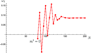
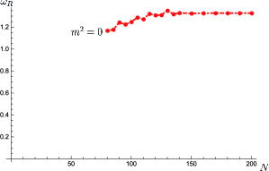
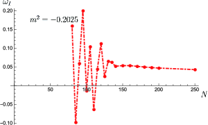
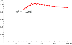
Figure 15: The plots of ${\omega}_{I}$ (left) and ${\omega}_{R}$ (right) vs. $N$ for $m^{2}=0,-0.2025$ (top, bottom) with the case $M=10^{-5}$ in Fig. 6. These show the convergence of the numerical results when $N$ is about $250$. As $m^{2}$ becomes negatively larger, $N$ needs to be higher to achieve the convergence and these cases are not included in this paper.

As the final remark, it would be straightforward to extend our formalism to more general perturbations with spins, including the (gravitational, spin 2) perturbations of the wormhole space-time itself. It would be interesting to study whether ring-down phases of natural wormholes can mimic those of black holes.

References

• (1) B. P. Abbott et al., Phys. Rev. Lett.  116, 241103 (2016).
• (2) B. P. Abbott et al., Phys. Rev. Lett.  119, 161101 (2017).
• (3) B. P. Abbott et al., Phys. Rev. Lett.  116, 221101 (2016).
• (4) E. Berti, V. Cardoso, and A. O. Starinets, Class. Quant. Grav.  26, 163001 (2009); R. A. Konoplya and A. Zhidenko, Rev. Mod. Phys.  83, 793 (2011).
• (5) T. Damour and S. N. Solodukhin, Phys. Rev. D 76, 024016 (2007).
• (6) V. Cardoso, E. Franzin, and P. Pani, Phys. Rev. Lett.  116, 171101 (2016); Erratum, Phys. Rev. Lett.  117, 089902 (2016).
• (7) R. A. Konoplya and C. Molina, Phys. Rev. D 71, 124009 (2005); R. A. Konoplya and A. Zhidenko, JCAP 1612, 043 (2016); K. K. Nandi, R. N. Izmailov, A. A. Yanbekov, and A. A. Shayakhmetov, Phys. Rev. D 95, 104011 (2017); P. Bueno, P. A. Cano, F. Goelen, T. Hertog, and B. Vercnocke, Phys. Rev. D 97, 024040 (2018); S. H. Volkel and K. D. Kokkotas, Class. Quant. Grav.  35, 105018 (2018); J. L. Blazquez-Salcedo, X. Y. Chew, and J. Kunz, Phys. Rev. D 98, 044035 (2018).
• (8) M. S. Morris and K. S. Thorne, Am. J. Phys. 56, 395 (1988).
• (9) M. Visser, Nucl. Phys. B 328, 203 (1989); Lorenzian wormholes: From Einstein to Hawking (AIP Press, Woodbury, USA, 1995).
• (10) M. B. Cantcheff, N. E. Grandi, and M. Sturla, Phys. Rev. D 82, 124034 (2010).
• (11) S. W. Kim and M.-I. Park, Phys. Lett. B 751, 220 (2015).
• (12) J. Y. Kim and M.-I. Park, Eur. Phys. J. C 76, 621 (2016).
• (13) P. Breitenlohner and D. Z. Freedman, Phys. Lett.  115B, 197 (1982); Ann. Phys.  144, 249 (1982); P. K. Townsend, Phys. Lett.  148B, 55 (1984); L. Mezincescu and P. K. Townsend, Annals Phys.  160, 406 (1985).
• (14) A. R. Gover, A. Shaukat, and A. Waldron, Nucl. Phys. B 812, 424 (2009); H. Lu and K. N. Shao, Phys. Lett. B 706, 106 (2011).
• (15) G. T. Horowitz and V. E. Hubeny, Phys. Rev. D 62, 024027 (2000).
• (16) B. Wang, C. Y. Lin, and E. Abdalla, Phys. Lett. B 481, 79 (2000); V. Cardoso and J. P. S. Lemos, Phys. Rev. D 64, 084017 (2001); E. Berti and K. D. Kokkotas, Phys. Rev. D 67, 064020 (2003).
• (17) D. Birmingham, I. Sachs, and S. N. Solodukhin, Phys. Rev. Lett.  88, 151301 (2002).
• (18) M. Born and L. Infeld, Proc. R. Soc. Lon. A 143, 410 (1934); ibid., 144, 425 (1934).
• (19) A. Garcia, H. Salazar, and J. F. Plebanski, Nuovo Cimento 84, 65 (1984); M. Demianski, Found. Phys. 16, 187 (1986); H. P. de Oliveira, Class. Quant. Grav. 11, 1469 (1994); D. A. Rasheed, hep-th/9702087; S. Ferdinando and D. Krug, Gen. Rel. Grav. 35, 129 (2003); R. G. Cai, D. W. Pang, and A. Wang, Phys. Rev. D 70, 124034 (2004); Y. S. Myung, Y.-W. Kim, and Y.-J. Park, Phys. Rev. D 78, 084002 (2008); S. Gunasekaran, R. B. Mann, and D. Kubiznak, JHEP 1211, 110 (2012); D. C. Zou, S. J. Zhang, and B. Wang, Phys. Rev. D 89, 044002 (2014); S. Fernando, Int. J. Mod. Phys. D 22, 1350080 (2013); S. Li, H. Lu, and H. Wei, arXiv:1606.02733 [hep-th].
• (20) S. Fernando and C. Holbrook, Int. J. Theor. Phys.  45, 1630 (2006).
• (21) R. G. Leigh, Mod. Phys. Lett. A 4, 2767 (1989); E. S. Fradkin and A. A. Tseylin, Phys. Lett. B 163, 123 (1985).
• (22) F. Calogero, J. Math. Phys.  10, 2191 (1969).
• (23) K. M. Case, Phys. Rev.  80, 797 (1950).
• (24) S. Moroz, Phys. Rev. D 81, 066002 (2010).
• (25) S. Chandrasekhar, The mathematical theory of black holes (Oxford University, New York, 1983).
• (26) A. Ohashi and M. A. Sakagami, Class. Quant. Grav.  21, 3973 (2004).
• (27) R. A. Konoplya, K. Murata, J. Soda, and A. Zhidenko, Phys. Rev. D 78, 084012 (2008).
• (28) R. Gregory and R. Laflamme, Phys. Rev. Lett.  70, 2837 (1993).
• (29) S. Yin, B. Wang, R. B. Mann, C. O. Lee, C. Y. Lin, and R. K. Su, Phys. Rev. D 82, 064025 (2010).
• (30) R. A. Konoplya, Phys. Rev. D 70, 047503 (2004); Y. Liu and B. Wang, Phys. Rev. D 85, 046011 (2012).
• (31) T. Moon, Y. S. Myung and E. J. Son, Eur. Phys. J. C 71, 1777 (2011).
• (32) U. H. Danielsson, E. Keski-Vakkuri, and M. Kruczenski, Nucl. Phys. B 563, 279 (1999).