Free electron laser in magnetically dominated regime: simulations with ONEDFEL code

Abstract

Using the ONEDFEL code we perform Free Electron Laser simulations in the astrophysically important guide-field dominated regime. For wigglers’ (Alfvén waves) wavelengths of tens of meters and beam Lorentz factor $\sim 10^{3}$, the resulting coherently emitted waves are in the centimeter range. Our simulations show a growth of the wave intensity over fourteen orders of magnitude, over the astrophysically relevant scale of $\sim$ few kilometers. The signal grows from noise (unseeded). The resulting spectrum shows fine spectral sub-structures, reminiscent of the ones observed in Fast Radio Bursts (FRBs).

1 Introduction: Free Electron Laser in astrophysical setting

Pulsars’ radio emission mechanism(s) eluded identification for nearly half a century ( Melrose, 2000; Lyubarsky, 2008; Eilek and Hankins, 2016). Most likely, several types of coherent processes operate in different sources (magnetars versus pulsars), and in different parts of pulsar magnetospheres (see  discussion in Lyutikov et al., 2016).

The problem of pulsar coherent emission generation has been brought back to the research forefront by the meteoritic developments over the last years in the field of mysterious Fast Radio Bursts (FRBs). Especially important was the detection of a radio burst from a Galactic magnetar by CHIME and STARE2 collaborations in coincidence with high energy bursts (CHIME/FRB Collaboration et al., 2020; Ridnaia et al., 2021; Bochenek et al., 2020; Mereghetti et al., 2020; Li et al., 2021). The similarity of properties of magnetars’ bursts to the Fast Radio Bursts gives credence to the magnetar origin of FRBs (even though the radio powers are quite different - there is a broad distribution).

The phenomenon of Fast Radio Bursts challenges our understating of relativistic plasma coherent processes to the extreme. In this case radio waves can indeed carry an astrophysically important amount of the energy. For example, radio luminosity in FRBs can match, for a short period of time, the macroscopic Eddington luminosity and exceed total Solar luminosity by many orders of magnitude. Still, the fraction emitted in radio remains small - this relatively small fraction of total energy that pulsars and FRBs emit in radio ($\sim 10^{-5}$ is typical) is theoretically challenging: simple order-of-magnitude estimates cannot be used. Emission production and saturation levels of instabilities depend on the kinetic details of the plasma distribution function.

Lyutikov (2021) developed a model of the generation of coherent radio emission in the Crab pulsar, magnetars and Fast Radio Bursts (FRBs) due to a variant of the free-electron laser (FEL) mechanism, operating in a weakly-turbulent, guide-field dominated plasma. This presents a new previously unexplored way (in astrophysical settings) of producing coherent emission via parametric instability.

A particular regime of the FEL (SASE - Self-Amplified Spontaneous Emission) micro-bunching is initiated by the spontaneous radiation. In the beam frame the wiggler and the electromagnetic wave have the same frequency/wave number, but propagate in the opposite direction. The addition of two counter-propagating waves creates a standing wave in the beam frame. The radiation energy density is smaller at the nodes of the standing wave: this creates a ponderomotive force that pushes the particles towards the nodes - bunches are created. These bunches are still shaken by the electromagnetic wiggler: they emit in phase, coherently.

Somewhat surprisingly, the FEL model in magnetically dominated regimes (Lyutikov, 2021) is both robust to the underlying plasma parameters and succeeded in reproducing a number of subtle observed features: (i) emission frequencies depend mostly on the scale $1/k_{w}$ of turbulent fluctuations and the Lorentz factor of the reconnection generated beam, Eq. (7); it is independent of the absolute value of the underlying magnetic field. (ii) The model explained both broadband emission and the presence of emission stripes, including multiple stripes observed in the High Frequency Interpulse of the Crab pulsar. (iii) The model reproduced correlated spectrum-polarization properties: the presence of narrow emission bands in the spectrum favors linear polarization, while broadband emission can have arbitrary polarization. The model is applicable to a very broad range of neutron star parameters: the model is mostly independent of the value of the magnetic field. It is thus applicable to a broad variety of NSs, from fast spin/weak magnetic field millisecond pulsars to slow spin/super-critical magnetic field in magnetars, and from regions near the surface up to (and a bit beyond of) the light cylinder.

The guide field dominance plays a tricky role in the operation of an FEL. On the one hand it suppresses the growth rate. But what turns out to be more important in astrophysical applications is that the guide field dominance helps to maintain beam coherence. Without the guide field, particles with different energies follow different trajectories in the magnetic field of the wiggler, and quickly lose coherence even for small initial velocity spread. In contrast, in the guide-field dominated regime all particles follow, basically, the same trajectory. Hence coherence is maintained as long as the velocity spread in the beam frame is $\Delta\beta\leq 1$.

A particularly relevant FEL regime is the SASE process - Self-Amplified Spontaneous Emission. Spontaneous emission is first produced due to incoherent single particle emission in a wiggler field. Then the beat between this spontaneous emission and the wiggler leads to the parametric resonance, whereby under certain conditions the electromagnetic field is further amplified. The SASE process has the right ingredients for the astrophysical applications, when no engineer can tune the parameters of the beam and of the wiggler.

Next we cite two features of work Lyutikov (2021) - growth rate and the Hamiltonian - which are particularly important for the present work, as they describe evolution of the instability and its saturation. Particle motion in the combined fields of the wiggler $B_{w}$, the EM wave $E_{EM}$ (both with wave vector $k_{w}^{\prime}$ in the beam frame) and the guide-field $B_{0}\gg E_{w},E_{EM}$ can be described by a simple ponderomotive Hamiltonian Lyutikov (2021)

$${\cal H}=\frac{\beta_{z}^{2}}{2}+\delta\left(\frac{E_{EM}}{B_{0}}\right)\left(\frac{\Omega_{0}}{k_{w}c}\right)\sin^{2}(k_{w}^{\prime}z)$$ (1)

($\beta_{z}$ is axial velocity; linearly polarized wiggler is assumed). The Hamiltonian formulation allows powerful analytical methods to be applied to the system (adiabatic invariant, phase space separatrix etc). This is especially important for the estimates of the non-linear saturation, one of the main goals of the present work.

The corresponding growth rate of the parametric instability is (Lyutikov, 2021, Eq. (62) ) is

$$\Gamma=\left(\left(\frac{E_{w}}{B_{0}}\right)\left(\frac{E_{EM}}{B_{0}}\right){\Omega_{0}}{k_{w}c}\right)^{1/2}\propto B_{0}^{-1/2}$$ (2)

It is mildly suppressed by the strong guide field.

2 Simulations with ONEDFEL and MINERVA codes

2.1 Model parameters

Let us next discuss the basic model parameters. (Unfortunately, there is some confusion in standard definitions used in literature.)

The model starts with an assumption that guiding magnetic field lines are perturbed by a packet of linearly polarized Alfvén waves of intensity $B_{w}$ and frequency $\omega$. The first parameter is dimensionless wave intensity. We chose notation $a_{0}$, which is standard in the laser community and sometimes used in the FEL community as well,

$$a_{0}=\frac{eB_{w}}{m_{e}c\omega}\gg 1$$ (3)

It should be remarked that in the FEL literature parameters $K$ and $a_{0}$ are often used interchangeably. In this paper, we follow the nomenclature used for $K$ in Eq. (2.4) below in Jackson (1975), parag. 14.7

For guide-field dominated regime another parameter is the relative intensity

$$\delta=\frac{B_{w}}{B_{0}}\ll 1$$ (4)

where $B_{0}$ is a guide field. We assume that the wave is relatively weak.

A (reconnection-generated) beam of particles with Lorentz factor $\gamma_{b}$ propagates along the rippled magnetic field in a direction opposite to the direction of Alfvén waves. In the frame of the beam the waves are seen with $k_{w}^{\prime}=2\gamma_{b}k_{w}$. In the guide-field dominated regime the cyclotron frequency associated with the guide field is much larger than the frequency of the wave in the beam frame, and the cyclotron frequency associated with the fluctuating field; hence

$$\Omega_{0}\gg k_{w}^{\prime}c,\Omega_{w}$$ (5)

where $\Omega_{0}=eB_{0}/(m_{e}c)$ is the cyclotron frequency (non-relativistic) of the guide field, $\Omega_{w}=eB_{w}/(m_{e}c)$ is the cyclotron frequency associated with the wiggler field.

Another important parameter, defined by (Jackson, 1975, parag. 14.7) is wiggler-undulator parameter

$$K=\delta\gamma_{b}$$ (6)

This parameter is related to the magnitude of the wiggler-induced oscillations in the beam trajectory, which is also related to the opening angle of the cone of the generated radiation. When $K\gg 1$ this oscillation is large and the pump field is sometimes referred to as a “wiggler”. In the opposite regime where $K\ll 1$ the pump field sometimes referred to as an “undulator”. In this paper, we will refer to the pump field as a wiggler throughout.

The $K$ parameter (6) is a product of two quantities, relative amplitude $\delta\ll 1$ and Lorentz factor $\gamma_{b}\gg 1$, so generally its values can be either large and small. A relativistically moving electron emits in a cone with opening angle $\Delta\theta\sim 1/\gamma$. In the $K\ll 1$ regime regime that opening angle is much larger than the variation in the bulk direction of emission at different points in the trajectory which is determined by the curvature of the guiding magnetic field. The radiation detected by an observer is an almost coherent superposition of the contributions from all the oscillations in the trajectory at a frequency

$$\omega_{C}=\gamma_{b}^{2}(ck_{w})\times\left\{\begin{array}[]{cc}4,&\mbox{EM wiggler}\\ 2,&\mbox{static wiggler}\end{array}\right.$$ (7)

We note that for$\gamma_{b}\gg 1$ static wigglers are nearly identical to electromagnetic wigglers except for the difference in the resonant frequency.

In the $K\gg 1$ regime the variations in the direction of emission is much larger than the angular width of the emission at any point in the trajectory. As a result, an observer located within angle $\leq\delta$ with respect to the overall guide field see periodic bursts of emission with typical frequency

$$\omega_{c}\approx\gamma_{b}^{2}K(ck_{w})$$ (8)

Since $K\gg 1$ in this regime, the resulting frequency is higher than that for the case where $K\ll 1$. In this paper, we work in the $K\ll 1$ regime which is the regime more typical of FELs.

Another terminology issue: here we contrast the term “Compton” with “curvature”, not with “Raman” regime, which is Compton-like scattering, but on collective plasma fluctuations.

In this paper we work in the regime $K\ll 1$ (this is the usual regime of FELs). The scattered frequency is then given by (7); below we drop the subscript $C$.

2.2 Applicability of 1D regime

There are a number of limitations to the 1D approximation used in the code ONEDFEL. The most important one is the curvature of the magnetic field lines over the amplification length. For $K\sim 1$, the typical emission angle is $\sim 1/\gamma_{b}$. Dipolar magnetic field line have a radius of curvature $R_{c}$ at dipolar coordinate $\{r,\theta_{d}\}$

$$\frac{R_{c}}{r}=\frac{\sqrt{2}r(3\cos(2\theta_{d})+5)^{3/2}}{3(5\sin(\theta_{d})+\sin(3\theta_{d}))}$$ (9)

Except for the points near the equator ($\theta_{d}\approx\pi/2$, $R_{c}/r\sim 1/3$), the radius of curvature is much larger than $r$, approximately

$$\frac{R_{c}}{r}\approx\frac{4}{3\theta_{d}},\,\theta_{d}\leq 1$$ (10)

The condition at the emission site

$$\frac{(\Delta r)}{R_{c}(r)}\leq\frac{1}{\gamma_{b}}$$ (11)

($(\Delta r)$ is growth length) restricts the operation of the FEL in the magnetospheres of neutron stars. Given the required Lorentz factor $\gamma_{b}\sim$ few $\times 10^{2}$, operation of the 1D FEL is restricted to $\theta_{d}/(r/R_{NS})\leq 10^{-2}$. For example, FEL is operational at $r\geq 10R_{NS}$ and $\theta_{d}\leq 0.1$ ( on the open field lines of the magnetosphere). Further out, at $r\geq$ few $\times 10^{2}R_{NS}$, FEL may operate in the most of the dipolar magnetosphere.

In addition, development of a Coronal Mass Ejection, accompanying magnetospheric FRBs, may lead to poneing of the ms from radii much smaller than the light cylinder  (Sharma et al., 2023). Particle motion along the resulting nearly-radial field lines is even better for phase coherence.

2.3 The codes

In this work we performed simulations of the interaction of a single-charged relativistic beam with the wiggler using FEL code ONEDFEL (Freund and Antonsen, 2023). ONEDFEL is time-dependent code that simulates the FEL interaction in one-dimension. The radiation fields are tracked by integration of the wave equation under the slowly-varying envelope approximation. As such, the wave equation is averaged over the fast time scale under the assumption that the wave amplitudes vary slowly over a wave period. The dynamical equations are a system of ordinary differential equations for the mode amplitudes of the field and the Lorentz force equations for the electrons which are integrated simultaneously using a 4th order Runge-Kutta algorithm. Time dependence is treated by including multiple temporal “slices” in the simulation which are separated by an integer number of wavelengths. The numerical procedure is that each slice is advanced from $z\to z+\Delta z$ separately by means of the Runge-Kutta algorithm. Time dependence is imposed as an additional operation by using the forward time derivative as an additional source term to treat the slippage of the radiation field with respect to the electrons. Slippage occurs at the rate of one wavelength per undulator period. The simplest way to accomplish this is to use a linear interpolation algorithm to advance the field from the $(i-1)$th slice to the $i$th slice. Using this procedure ONEDFEL can treat electron beams and radiation fields with arbitrary temporal profiles and it is possible to simulate complex spectral properties.

Simulations, effectively, work in the lab frame, The general set-up consists of

• guide magnetic field  $B_{0}$ (as strong as numerically possible);

• a wiggler with wave number $k_{w}$ and relative amplitude $\delta=B_{w}/B_{0}\ll 1$ is as EM wave (with adiabatic turning-on); wiggler’s frequency in the beam frame is below the cyclotron frequency associated with the guide field, $\omega_{w}\sim\gamma_{b}\ll\omega_{B_{0}}$ (but can be comparable to the cyclotron frequency of the wiggler, $\omega_{B_{w}}$);

• charged beam with “solid” (dead) neutralizing background; the corresponding Alfvén wave is relativistic, $v_{A}\sim c$. The beam is initially propagating along the magnetic field (no gyration)

• pulse duration is much longer than the wiggler wavelength.

By using a pure EM wave, and not as a self-consistent Alfvén wave, eliminates complications related to setting the correct particle currents. In the highly magnetized regime $\sigma\gg 1$ Alfvén waves are nearly luminal.

3 Results

In simulating the magnetar magnetosphere environment we consider an electron beam propagating along the magnetic field in the presence of a plane-polarized electromagnetic wave. The basic parameters are shown in Table 1. We consider a mono-energetic 50 MeV beam over a bunch length/charge of 1.8 $\mu$s/5.9 mC with a peak current of 5 kA. The beam plasma frequency corresponding to a 5 kA beam with a radius of 100 cm is about 1.6 kHz. The electromagnetic undulator is taken to have a period of 100 m and an amplitude of 0.01 kG. The excited radiation, therefore is also plane-polarized. We study the interaction for various values of the axial field so that the resonant wavelength will vary with the axial field.

Beam Energy	50 MeV
Peak Current	5000 A
Bunch Duration	1.8 $\mu$s
Beam Radius	100 cm
Pitch Angle Spread	0
Period	100 m
Amplitude	0.01 kG
Polarization	Planar
Axial Magnetic Field ($B_{0}$)	Variable
Amplitude	Variable

Table 1: Parameters of simulations

.

The parameters of simulations nearly match the real physical condition (except the value of the guide field): for a beam Lorentz factor $\gamma_{b}\sim 100$ and a wiggler length $\lambda_{w}\sim 100$ meters the resonant wavelength is a few centimeters. These values are close to the real scales we expect in neutron star magnetospheres. As mentioned previously, the guide field is below that expected but the numerical simulation becomes more and more computationally challenging as the resonant linewidth becomes narrower for high guide fields. However, the wavelength becomes independent of the guide field (Fig. 1). In this particular example, over a few kilometers (also a realistic physical value) the intensity grows by fourteen orders of magnitude and reaches saturation.

3.1 Steady-state runs

Using steady-state (i.e., time independent) ONEDFEL simulations, we have studied the variation in the resonant wavelength with increases in the magnetic field. As shown in Fig. 1, the resonant wavelength for the FEL interaction decreases from about 0.25 m for a magnetic field of 0.15 kG to 0.053 m when the magnetic field increases to 0.20 kG. We observe that the curve is approaching an asymptote as $B_{0}$ increases past 0.20 kG. This means that the resonant wavelength will remain relatively constant as the magnetic field increases above this value and we expect that the interaction properties will not change significantly for still higher field levels. This is important because simulations become increasing challenging as the field increases beyond this point. The variation in the saturated power and saturation distance (when starting from noise) are shown in Fig. 1 for $B_{0}=0.20$ kG. Here we observe that the full width of the gain band extends from about 0.051 m to 0.056 m and the optimal wavelength, corresponding to the shortest saturation distance is 0.053 m (as indicated in Fig. 1) and that the decreases rapidly as the wavelength increases within this gain band.

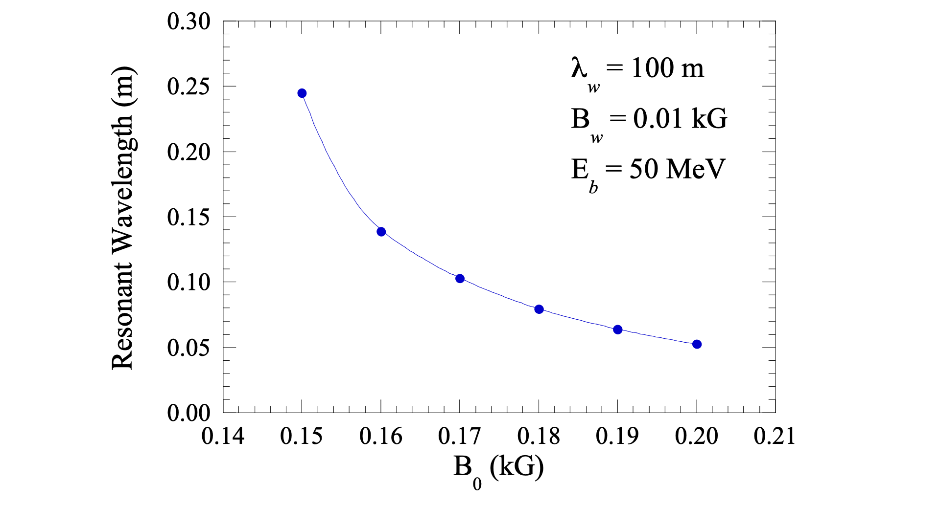
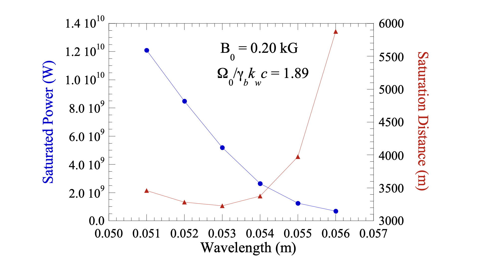
Figure 1: Steady-state runs. Left panel: Variation in the FEL resonant wavelength with magnetic field in the Group II regime. Right panel: The saturated power and saturation distance versus wavelength for $B_{0}=0.2$ kG.

3.2 Time-dependent simulations

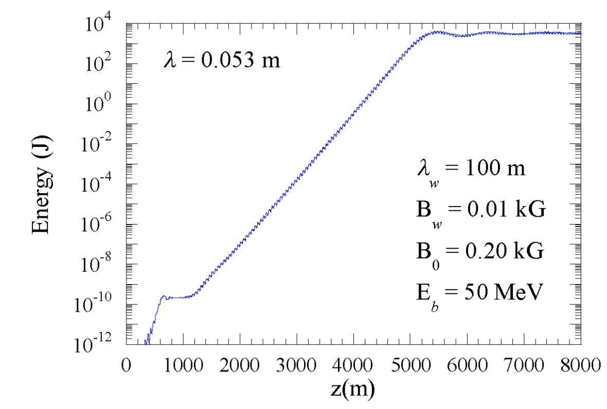
Figure 2: FEL power as a function of distance. We observe a growth of the EM signal over $\sim$ fourteen orders of magnitude, from noise (no seeding)! (over a scale of $\sim$ few kilometers - realistic neutron star setting).

Next, we ran time-dependent simulations using ONEDFEL. Simulations were conducted to determine the resonant wavelengths for different values of the axial magnetic field. Note that while these are 1D simulations, we need to specify the beam radius in order to determine the current density and beam plasma frequency.

Our results are plotted in Fig. 2. Importantly, the signal evolves from noise - there is no seeding. The simulations nearly match the real physical condition: for beam Lorentz factor $\gamma\sim 100$ and wiggler length $\lambda_{w}=100$ meters the resonant wave length is few centimeters! These values are close to the real scales we expect in neutron star magnetospheres!). The guide field is below that of the expected, though. For high guide fields the procedure becomes more and more computationally challenging as the resonant line becomes narrower. Over a scale of few kilometers (also a realistic physical value) the intensity grows by fourteen orders of magnitude, reaching saturation.

The resulting spectral structure is most revealing, Fig. 3, left panel. We find that the pulse has a complicated internal spectral structure, which is a natural property of a SASE FEL. It is evident that the spectral width of the central spike is less than 1% (FWHM).

This complicated internal structure resembles what is indeed seen in Fast Radio Bursts, Fig. 3, right panel. FRBs display a wide variety of complex time-frequency structures (Ravi et al., 2016; Michilli et al., 2018), including strong modulations in both frequency and time (with characteristic bandwidth of $\sim 100$ kHz.)

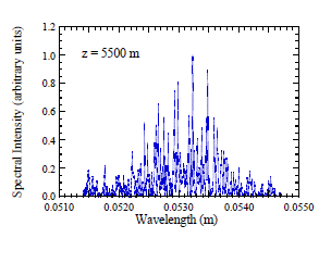
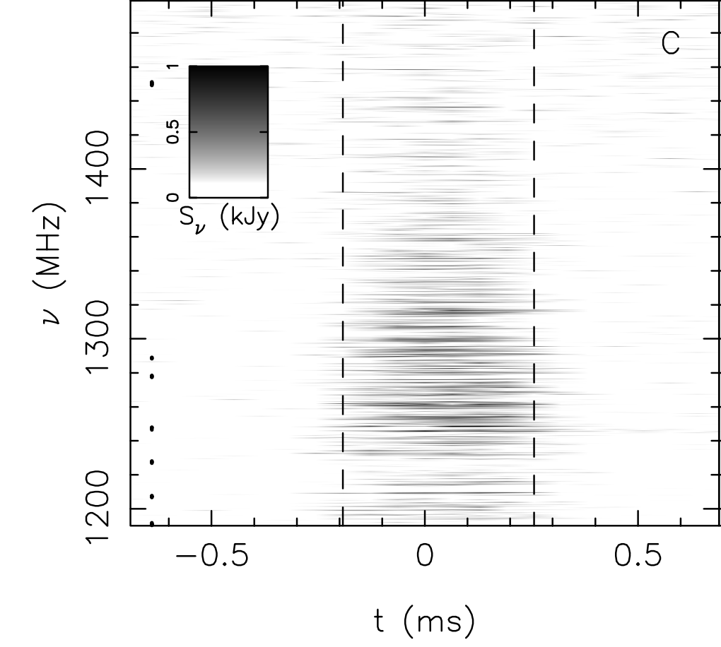
Figure 3: Left panel: Time-dependent simulations of the FEL with ONEDFEL showing complicated internal spectral structure of FEL in SASE regime. Right panel: Dynamic spectrum of FRB150807 (Ravi et al., 2016) showing strong modulations in both frequency and time. (Time and frequency structures are inter-dependent in the de-dispersion procedures.)

3.3 Connection to CARM regime

Particle-wave interaction may lead to the excication of the cycltron motion and ensuing azimuthal bunching of emitting electrons. This will take the us into the Cyclotron Auto Resonance Maser (CARM regime). In this case, the resonant wavelength is governed by the axial velocity of the electron beam and, for fixed beam energy and undulator parameters, this will vary with the axial field. For given wiggler and axial magnetic field parameters, there are two classes of trajectories: Group I and Group II which are illustrated in Fig. 4 for a magneto-static wiggler (Freund and Drobot, 1982). Group I trajectories are generally found in the weak axial field regime below the magneto-resonance, $\Omega_{0}\leq\gamma_{b}k_{w}c$, and Group II trajectories occur in the strong axial field regime where $\Omega_{0}\gg\gamma_{b}k_{w}c$. We are most concerned with Group II trajectories which we expect to be relevant to the conditions in magnetar magnetospheres.

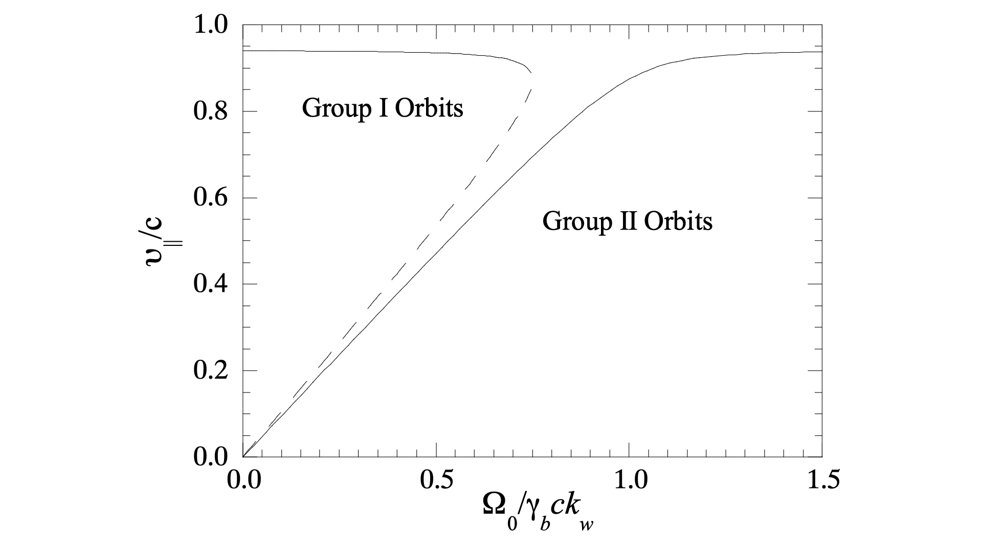
Figure 4: Illustration of the variation in the axial velocity with the axial magnetic field for Group I and Group II trajectories (Freund and Antonsen, 2023).

As shown in Fig. 4, the axial velocity increases with increasing magnetic field in the Group II regime which implies that the FEL resonant wavelength decreases with increasing magnetic field.

We remark that there are two possible interactions of an electron beam streaming along the field lines corresponding to the FEL resonance and that of a cyclotron auto-resonance maser (CARM). The ratio of the resonant frequencies of these two interaction mechanisms is given by

$$\frac{\omega_{CARM}}{\omega_{FEL}}=\frac{\Omega_{0}}{\gamma_{b}k_{w}c},$$ (12)

so that the FEL resonance is found at a lower frequency than that for the CARM for strong axial guide fields in the Group II regime. For the parameters of interest here, the magneto-resonance is found for an axial field of about 0.10 kG as shown in Fig. 5. We are primarily concerned here with the strong axial field regime.

This is a separate, and possibly astrophysically important emission mechanism. We leave the analysis of CARM regime to a separate future investigation.

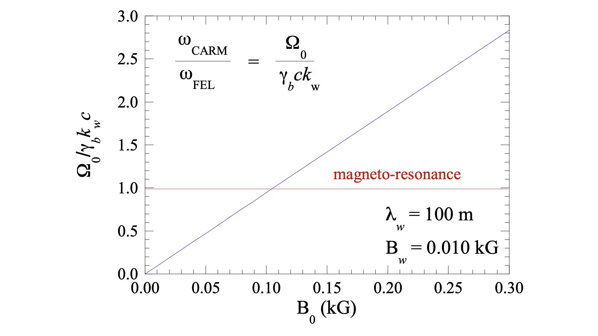
Figure 5: Plot showing the variation in $\Omega_{0}/\gamma_{b}k_{w}c$ versus the axial field showing that Group I orbits are found when $B_{0}\leq 0.10$ kG and Group II orbits when $B_{0}\geq$ 0.10 kG.

4 Conclusion

In this work we numerically study operation of Free Electron Laser in the astrophysically important guide-field dominated regime. In this regime particles mostly slide along the dominant guiding magnetic field  and experience ${\bf E}\times{\bf B}$ drift in the field of the wiggler. Our parameters (energy of the beam, wavelength of the wiggler) closely match what is expected in the magnetospheres of neutron stars. The value of the guide field is, though, much smaller than expected. However, we verified that the wavelength becomes independent of the guide field, Fig. 1.

Our results are encouraging. First, we see unseeded growth over 14 orders of magnitude over the real physical scale of $\sim$ few kilometers. It is expected that the real magnetospheres are much “noisier“, with mild level of intrinsically present turbulence. The presence of such turbulent Alfvén waves will provide seeds to jump-start the operation of the FEL.

The most intriguing result is, perhaps, the fine spectral structure, Fig. 3, that qualitatively matches observations. Such fine structure is an inherent property of SASE FEL, as different narrow modes are amplified parametrically.

Limitations of our approach include:

• One-dimensional approximation. In this case we neglect curvatures of the magnetic field lines, and corresponding particles’ trajectories. We plan to address this in a separate work, using MINERVA code.

• The saturation level will be affected by the higher guiding field. For a single quasi-monochromatic wave the ponderomotive potential (1) increases linearly with EM wave intensity $E_{w}$, while energy density of EM waves increases quadratically $\propto E_{w}^{2}$. The balance is achieved at

  $$\frac{E_{EM}}{E_{w}}=\frac{\omega_{p,b}^{2}}{k_{w}c\Omega_{0}},$$ (13)

  where $\omega_{p,b}$ is beam plasma density. This is an estimate of the saturation level of the EM waves in the beam frame.

• We have not addressed the energy spread in the beam. It is expected that in the guide-field dominated regime the operation of FEL is much more tolerant to the beam spread Lyutikov (2021) since in this regime the particle trajectory is independent of energy. In the broad-band case the saturation will be determined $\sim$ by a (random phase) quasilinear diffusion. In this regime the growth rate of the EM energy of the wave due to the development of the parametric instability, Eq. (2), will be balanced by the particle diffusion (random phases!) in the turbulent EM field (the diffusion coefficient $\propto E_{w}^{2}$).

• Coherence of the wiggler. We assumed purely monochromatic wiggler. Spectral spread of the wiggler will tend to reduce the FEL efficiency.

We plan to address theses issues in a future publication.

This work had been supported by NASA grants 80NSSC17K0757 and NSF grants 1903332 and 1908590.

References

- Melrose (2000) D. B. Melrose, in IAU Colloq. 177: Pulsar Astronomy - 2000 and Beyond, edited by M. Kramer, N. Wex, and R. Wielebinski (2000), vol. 202 of Astronomical Society of the Pacific Conference Series, pp. 721–+.
- Lyubarsky (2008) Y. Lyubarsky, in 40 Years of Pulsars: Millisecond Pulsars, Magnetars and More, edited by C. Bassa, Z. Wang, A. Cumming, and V. M. Kaspi (2008), vol. 983 of American Institute of Physics Conference Series, pp. 29–37.
- Eilek and Hankins (2016) J. A. Eilek and T. H. Hankins, Journal of Plasma Physics 82, 635820302 (2016), 1604.02472.
- Lyutikov et al. (2016) M. Lyutikov, L. Burzawa, and S. B. Popov, MNRAS 462, 941 (2016), 1603.02891.
- CHIME/FRB Collaboration et al. (2020) CHIME/FRB Collaboration, B. C. Andersen, K. M. Bandura, M. Bhardwaj, A. Bij, M. M. Boyce, P. J. Boyle, C. Brar, T. Cassanelli, P. Chawla, et al., Nature 587, 54 (2020), 2005.10324.
- Ridnaia et al. (2021) A. Ridnaia, D. Svinkin, D. Frederiks, A. Bykov, S. Popov, R. Aptekar, S. Golenetskii, A. Lysenko, A. Tsvetkova, M. Ulanov, et al., Nature Astronomy 5, 372 (2021), 2005.11178.
- Bochenek et al. (2020) C. D. Bochenek, V. Ravi, K. V. Belov, G. Hallinan, J. Kocz, S. R. Kulkarni, and D. L. McKenna, Nature 587, 59 (2020), 2005.10828.
- Mereghetti et al. (2020) S. Mereghetti, V. Savchenko, C. Ferrigno, D. Götz, M. Rigoselli, A. Tiengo, A. Bazzano, E. Bozzo, A. Coleiro, T. J. L. Courvoisier, et al., ApJ 898, L29 (2020), 2005.06335.
- Li et al. (2021) C. K. Li, L. Lin, S. L. Xiong, M. Y. Ge, X. B. Li, T. P. Li, F. J. Lu, S. N. Zhang, Y. L. Tuo, Y. Nang, et al., Nature Astronomy (2021), 2005.11071.
- Lyutikov (2021) M. Lyutikov, ApJ 922, 166 (2021), 2102.07010.
- Jackson (1975) J. D. Jackson, Classical electrodynamics (1975).
- Sharma et al. (2023) P. Sharma, M. V. Barkov, and M. Lyutikov, MNRAS 524, 6024 (2023), 2302.08848.
- Freund and Antonsen (2023) H. P. Freund and T. M. Antonsen, Principles of Free-electron Lasers (Springer Nature Switzerland, 4rd Edition, 2023).
- Ravi et al. (2016) V. Ravi, R. M. Shannon, M. Bailes, K. Bannister, S. Bhandari, N. D. R. Bhat, S. Burke-Spolaor, M. Caleb, C. Flynn, A. Jameson, et al., Science 354, 1249 (2016), 1611.05758.
- Michilli et al. (2018) D. Michilli, A. Seymour, J. W. T. Hessels, L. G. Spitler, V. Gajjar, A. M. Archibald, G. C. Bower, S. Chatterjee, J. M. Cordes, K. Gourdji, et al., Nature 553, 182 (2018), 1801.03965.
- Freund and Drobot (1982) H. P. Freund and A. T. Drobot, Physics of Fluids 25, 736 (1982).