Relativistic coronal mass ejections from magnetars

Abstract

We study dynamics of relativistic Coronal Mass Ejections (CMEs), from launching by shearing of foot-points (either slowly - the “Solar flare” paradigm, or suddenly - the “star quake” paradigm), to propagation in the preceding magnetar wind. For slow shear, most of the energy injected into the CME is first spent on the work done on breaking through the over-laying magnetic field. At later stages, sufficiently powerful CMEs may experience “detonation” and lead to opening of the magnetosphere beyond some equipartition radius $r_{eq}$, where the energy of the CME becomes larger than the decreasing external magnetospheric energy. Post-CME magnetosphere relaxes via formation of a plasmoid-mediated current sheet, initially at $\sim r_{eq}$ and slowly reaching the light cylinder (this transient stage has much higher spindown rate and may produce an “anti-glitch”). Both the location of the foot-point shear and the global magnetospheric configuration affect the frequent-and-weak versus rare-and-powerful CME dichotomy - to produce powerful flares the slow shear should be limited to field lines that close near the star. After the creation of a topologically disconnected flux tube, the tube quickly (at $\sim$ the light cylinder) comes into force-balance with the preceding wind, and is passively advected/frozen in the wind afterward. For fast shear (a local rotational glitch), the resulting large amplitude Alfven waves lead to opening of the magnetosphere (which later recovers similarly to the slow shear case). At distances much larger than the light cylinder, the resulting shear Alfven waves propagate through the wind non-dissipatively. Implications to Fast Radio Bursts are discussed.

1 Introduction

Magnetars, a class of highly magnetized neutron stars, produce X-ray and $\gamma$-ray bursts (Thompson & Duncan, 1995; Komissarov & Barkov, 2007; Mereghetti, 2008; Kaspi & Beloborodov, 2017; Usov, 1992), and occasional giant flares (Palmer et al., 2005; Hurley et al., 2005). Discoveries related to Fast Radio Bursts (Petroff et al., 2019; Cordes & Chatterjee, 2019), especially simultaneous observations of radio and X-ray bursts from a magnetar (CHIME/FRB Collaboration et al., 2020; Ridnaia et al., 2021; Bochenek et al., 2020; Mereghetti et al., 2020) renewed interest in the dynamics of magnetar’s explosions.

To set-up the stage, we first qualitatively divide FRB models into two types - magnetospheric and wind models. Also qualitatively we divide magnetar flares’ models into Solar flare paradigm and Starquake paradigm, with a clear understanding that the actual separation of models is/may not be as clearly defined.

In the case of FRBs, one set of theories, advocates that FRBs are magnetospheric events (e.g.  Lyutikov, 2003; Popov & Postnov, 2013; Lyutikov et al., 2016; Lyutikov & Popov, 2020). Alternative suggestion is generation of FRBs in the wind or in the wind termination shock (e.g.  Lyubarsky, 2014; Beloborodov, 2017; Metzger et al., 2019; Thompson, 2022; Khangulyan et al., 2022; Barkov & Popov, 2022). Observations of contemporaneous magnetar X-ray flares and FRB strengthened the evidence for magnetospheric loci (as argued by Lyutikov & Popov, 2020); the detection of sub-second periodicity (CHIME/FRB Collaboration et al., 2022) leaves little doubt in our view. Recent detection of anti-glitch in FRB-associated magnetar Younes et al. (2022) is also consistent with the magnetospheric model, see Lyutikov (2013).

The wind models of FRBs appeal to the generation of strong shock, or magnetic shell that propagates through the wind. As we demonstrate in the present paper the assumption of strong shock/magnetic shell propagating through the wind is incorrect: the magnetic shells can naturally come into force balance near the light cylinder, and are then passively advected with the wind. We model quite a small magnetosphere radius $R_{LC}=5R_{NS}$. It allows to keep pressure balance due to small Lorentz factors of the flow. In the case of larger dynamical range (1$0^{4}$) it can be not so. acceleration of the blob inside magnetosphere up to $\Gamma>10$ will leads to lose of the casual connection and blob can escape in strongly unbalanced conditions and form explosion like solution in the wind zone.

As for magnetars’ flares, the Solar flare paradigm for magnetar explosions (Lyutikov, 2006, 2015) argues that the underlying mechanism that causes magnetars’ flares may be similar to those operating in the solar corona. According to the model, GFs are magnetospheric events. Alternative view is that magnetar flares are crustal events (Thompson & Duncan, 1995).

In the Solar flare paradigm the energy that will eventually power magnetar flares is first stored inside the neutron star right following the core-collapse of the progenitor star. Slowly over time, hundreds to thousands of years, the internal magnetic twist is pushed into the magnetosphere via Hall (electron-MHD) drift (Goldreich & Reisenegger, 1992; Gourgouliatos et al., 2013; Wood et al., 2014), gated by slow, plastic deformations of the neutron star crust (Lyutikov, 2015). This leads to gradual twisting of the external magnetospheric field lines, on time scales much longer than the magnetar’s GF, and creates active magnetospheric regions similar to the Sun’s spots. As more and more current is pushed into the magnetosphere, it eventually reaches a point of dynamical instability. The loss of stability leads to a rapid restructuring of magnetic configuration, on the Alfven crossing time scale, to the formation of narrow current sheets, and to the onset of magnetic dissipation. As a result, a large amount of magnetic energy is converted into the kinetic and bulk motion and radiation (Lyutikov, 2003; Komissarov et al., 2007; Ripperda et al., 2019; Yuan et al., 2020). The coherent emission may be produced due to some kind of plasma instability, e.g.  via the Free Electron Laser mechanism (Lyutikov, 2021). Perhaps the best argument in favor of the “Solar flare paradigm” is that the observed sharp rise of $\gamma$-ray flux during GF, on a time scale similar to the Alfvén crossing time of the inner magnetosphere, which takes $\sim 0.25$ msec (Palmer et al., 2005). This unambiguously points to the magnetospheric origin of GFs (Lyutikov, 2006). Since in the Solar flare paradigm, GFs are magnetospheric events, no large baryonic loading is expected in the ensuing outflows.

Another model of magnetars’ flares, which we call the Starquake model of Thompson & Duncan (1995, 2001) (though the “starquake” is not used in these papers - we thank Chis Thompson for pointing this out - we use this terms as a classification marker; the models do appeal to crustal faults) , whereas sudden fraction of the crust leads to fast motion of the magnetic foot-points. (Levin & Lyutikov, 2012, criticized this set-up: even if the elastic properties of the crust allow the creation of a shear crack, the strongly sheared magnetic field around the crack leads to a back-reaction from the Lorentz force which does not allow large relative displacement of the crack surfaces.)

For the present purposes, the difference between slow shear of the Solar flare and fast shear of the Starquake models is that for the slow shear the whole magnetosphere remains in the causal contact, while the fast shear corresponds to a packet of Alfvén waves generated by the foot-point motions. We emphasize that our separation of models into Solar flare - Starquake clearly misses many details and is introduced here to highlight the two different dynamics regimes in the ensuing discussion.

In the present paper we seek answers to the two sets of questions, one related to launching the CMEs from the magnetosphere, and the second related to the propagation of the resulting structures through the wind: (i) how the model of sheared/inflated magnetic flux tubes in the Sun (Antiochos et al., 1999) transports into relativistic highly magnetized regime; (ii) what is the role of the light cylinder in generating the CMEs; (iii) what underlying physical parameters distinguish magnetars’ giant flares, from the less energetic bursts; (iv) what is the dynamics of magnetospheric perturbation as they enter the wind. By the FRB-magnetar association, these question may carry the answer to why FRBs are different? Investigations are done with the code PHAEDRA (Parfrey et al., 2012), Appendix A. The code invokes force-free electrodynamics, an appropriate limit for the study of neutron star magnetosphere, considering their extremely high magnetic field. In this limit, hydrodynamic forces can be safely neglected and therefore the electromagnetic Lorentz force can be approximated as zero.

The plan of the paper is as follows. In §2 we describe theoretical expectations that would guide us through the following research. In §3 we describe the code. In §4 we concentrate on the inner-most dynamics of the CMEs, neglecting rotation/presence of the light cylinder. In §5 (slow shear) we adapt a model of generation of Solar CMEs by Antiochos et al. (1999, 2007) to relativistic rotating magnetospheres  of neutron stars. In §6 (fast shear) we consider dynamics of a “ glitched magnetosphere” - when a part of the neutron star’s crust experience sudden change in the rotational angular velocity. In §7 we consider dynamics, from the magnetospheres to the wind, of an ejected magnetic flux tube.

2 Magnetar’s CMEs

2.1 The Solar Flare paradigm

Coronal mass ejections (CMEs) are the most explosive events in our solar system and have been long studied in solar physics (Vourlidas et al., 2002; Forbes, 2000). According to the model of Solar flares by Antiochos et al. (1999, 2007), the underlying cause of the manifestations of solar activity - CMEs, eruptive flares and filament ejections - is the disruption of a force balance between the upward pressure of the strongly sheared field of a filament channel and the downward tension of a potential (non-current carrying) overlying field. Thus, an eruption is driven solely by the magnetic free energy stored in a closed, sheared magnetic field that opens toward infinity during a CME. Initially, the magnetic field has a complicated multipolar topology while reconnection between a sheared arcade and neighboring flux systems triggers the eruption. We also mention an important Aly’s theorem, that open topologies have the largest energy given poloidal magnetic field distribution on the surface (Aly, 1991). The presence of the light cylinder change this picture: if an arc reaches the light cylinder it will become open.

We first explore models of magnetar giant flares based on the same paradigm as Solar Flares and Coronal Mass Ejections (CME) (Antiochos et al., 1999, 2007), that they are driven by slow surface shear leading to catastrophic rearrangement of the neutron star’s magnetospheric fields.

The principal difference between Solar and magnetar CMEs is that the magnetar plasma is relativistic and strongly magnetized, with Alfven velocity of the order of the speed of light. Perhaps it is more correct to them Coronal Flux Ejections (Jens Mahlmann, priv. comm.), but we keep the more familiar notation of a CME. In addition, presence of a light cylinder play the most important part in the generation of CMEs in magnetars, if compared with non-rotating calculations of (Antiochos et al., 1999, 2007, the light cylinder is the analogue of the Alfven surface in rotating stars).

Through numerical experiments we found that several complementary ingredient control the overall dynamics of the generation of CMEs in magnetars: global magnetospheric structure, rotation, and the location of foot-point shear. To make the following discussion clear the term “shearing” refers to the dynamical motion of magnetic foot-points.

We first study step-by-step different global configurations and different shearing prescriptions. In Appendix A we study separately/reproduce analytical results for separate “ingredients” of the model: (ii) Sheared non-rotating magnetospheres, Appendix 4.1; (ii) Rotating stars with no foot-point shearing, Appendix C and in particular Michel’s solution, Fig. 24.

2.2 Theoretical expectations

2.2.1 The set-up

Let us first discuss dynamics of a topologically isolated flux tubes/magnetic blobs (called CME below) injected deep within a magnetosphere, so that the presence of a light cylinder is not important. Consider an injected isolated magnetic structure - two possible geometries include a magnetic flux tube and magnetic ball. Let the injection occur near the stellar surface with typical size $R_{CME,0}\leq R_{NS}$ and associated energy $E_{CME,0}$, Table 1. The magnetic field inside the CME is of the order of the surface magnetic field $B_{0}$, so that initially the CME is just slightly unbalanced - internal magnetic field matches approximately the magnetospheric field. The gradient of the external field pushes the CME out.

Model	flux tube	small CME	large CME $(r=R_{CME})$
Initial volume of CME	$2\pi R_{NS}\times\pi R_{CME,0}^{2}$, flux tube	$(4\pi/3)R_{CME,0}^{3}$, sphere	$(4\pi/3)R_{CME,0}^{3}$, sphere
injected energy $E_{CME,0}$	$2\pi R_{NS}R_{CME,0}^{2}{B_{0}^{2}}/{(8\pi)}$	$(4\pi/3)R_{CME,0}^{3}{B_{0}^{2}}/{(8\pi)}$	$(4\pi/3)R_{CME,0}^{3}{B_{0}^{2}}/{(8\pi)}$
CME’s linear size at $r$ $R_{CME}/R_{CME,0}$	$\left(\frac{r}{R_{NS}}\right)^{3/2}$	$\left(\frac{r}{R_{NS}}\right)^{3/2}$	$\left(\frac{r}{R_{NS}}\right)^{3}$
energy $E_{CME}/E_{CME,0}$ at $r$	$\left({R_{NS}}/{r}\right)^{2}$	$\left({R_{NS}}/{r}\right)^{3/2}$	$\left({R_{NS}}/{r}\right)$
Equipartition radius $r_{eq}/R_{NS}$	$\eta_{CME}^{-1}$	$\eta_{CME}^{-2/3}$	$\eta_{CME}^{-2/3}$
Energy remaining at $r_{eq}$	$\eta_{CME}^{2}$	$\eta_{CME}$	$\eta_{CME}$

Table 1: Typical scales for dynamics of CME injected within the magnetosphere. Only small fraction of the injected energy remains within the CME after it escapes from the magnetosphere.

An important parameter is the total magnetic energy of the magnetosphere,

$$E_{B,NS}\sim B_{0}^{2}R_{NS}^{3}$$ (1)

Naturally, the injected energy is much smaller than the total energy,

$$\eta_{CME}=\frac{E_{CME,0}}{E_{B,NS}}.$$ (2)

Conservation of the magnetic flux within CME plays the most important role. The injected flux is

$$\Phi_{B}\sim B_{0}R_{CME,0}^{2}={\rm Const}=B_{CME}R_{CME}^{2}$$ (3)

It is conserved during evolution. Thus, magnetic field inside is

$$B_{CME}=B_{0}\left(\frac{R_{CME,0}}{R_{CME}}\right)^{2}$$ (4)

We can then identify three different geometrical case: (i) flux tube (a toroidally-symmetric configuration), (ii) small magnetic ball (spherical ball displaced from the center); (iii) large magnetic ball ($R_{CME,0}\sim R_{NS}$) (centered ball). In the “large magnetic ball” case the quasi-spherical injected structure is of order of the neutron star from the beginning.

Importantly, we can then identify three regimes for the dynamics of the CME: (i) “breaking-out”; (ii) “detonation”; (iii) magnetospheric recovery; (iii) CME’s expansion in the wind, Figs. 1. During the early “breaking-out” phase the CME expands while doing work on the overlaying magnetic field. As a result, the energy of the CME reduces dramatically, Table 1. During “detonation” stage the CME expands nearly freely, opening the magnetosphere. After the CME’s break-out, the magnetosphererecovers by forming a current sheet, while the CME is mostly passively advected with the wind.

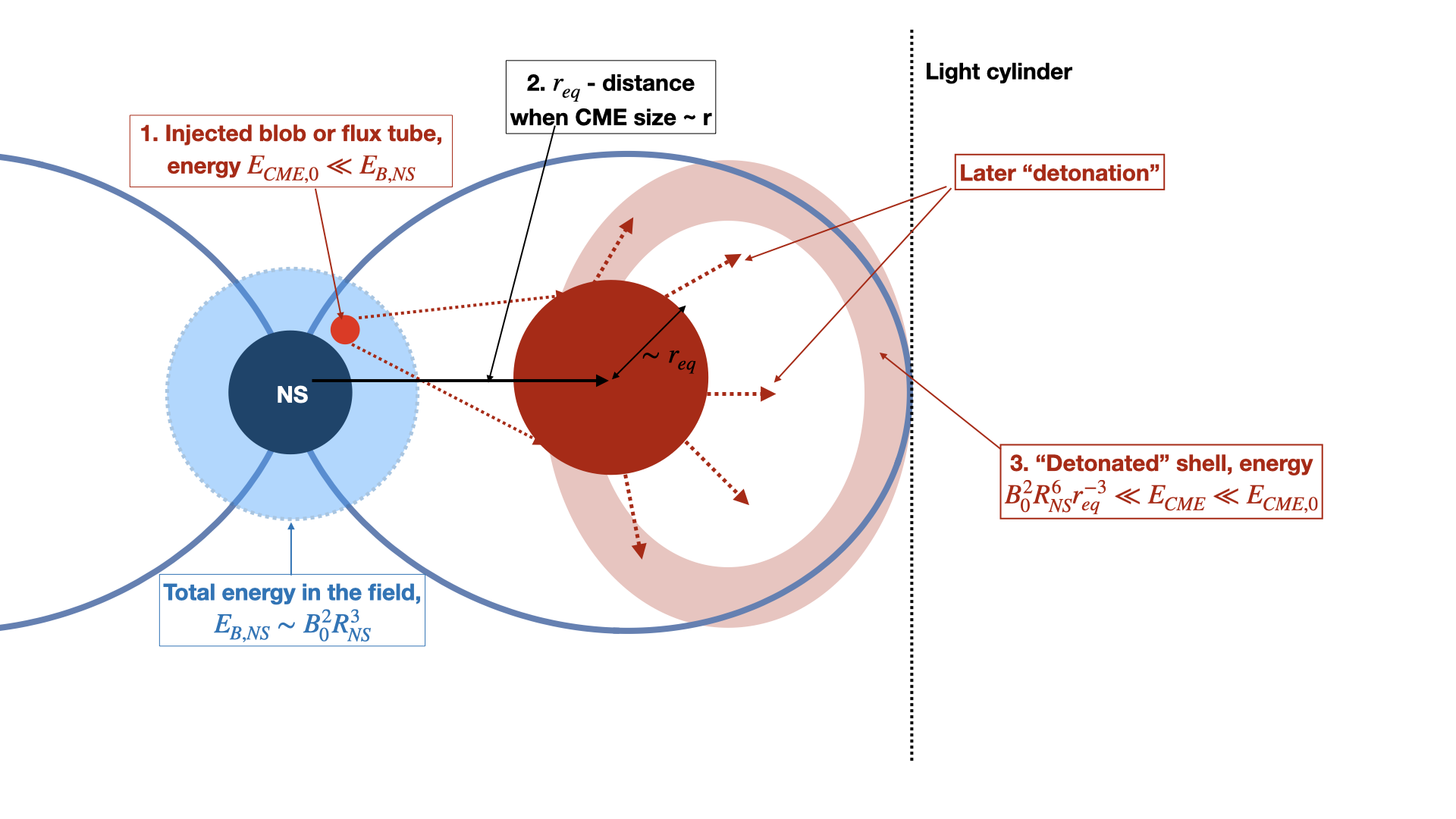
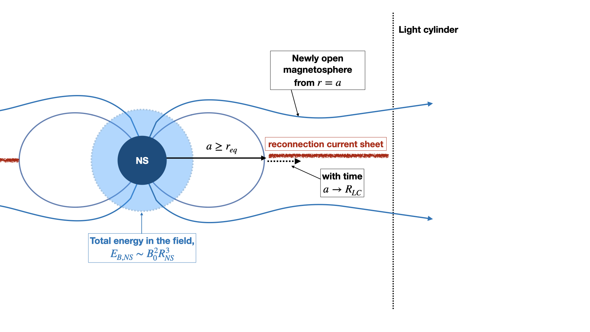
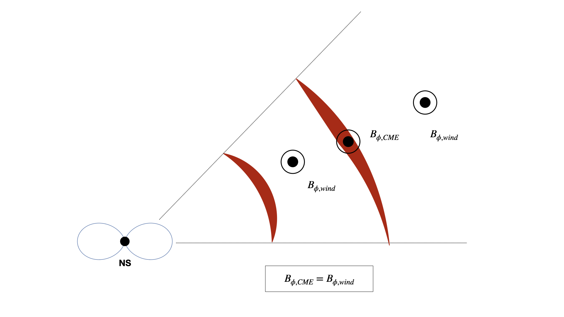
Figure 1: CME dynamics inside the magnetosphere and in the wind. Top panel: A CME, a flux tube or magnetic blob, carrying initial energy $E_{CME,0}$ is released near the surface. The energy of the CME is much smaller than the total magnetic energy of the magnetosphere, $E_{CME,0}\ll E_{B,NS}$. As the CME expands it is doing work on the over-laying magnetic field, and loses energy. Sufficiently powerful CME may still reach a size comparable to the local distance to the star $r_{eq}$ (while still within the light cylinder). After that the injected structure would expand quasi-spherically, opening field lines beyond $r_{eq}$. Central panel: post explosion relaxation. Generation of CME lead to opening of the magnetosphere at $r_{eq}\leq R_{LC}$. The post-CME magnetosphere recovers by forming a current sheet from $r_{eq}$ to $R_{LC}$. Bottom panel: CME in the wind. A flux tube is injected within the magnetosphere, CME first expands with the magnetosphere, losing energy doing work on the magnetospheric fields to break out, coming to a force balance near the light cylinder, and then is advected passively within the wind as a shell of constant radial and lateral extension.

2.2.2 The “breaking-out” stage

At the “breaking-out” stage the internal magnetic field (4) matches the magnetospheric field at the location of the CME,

$$B_{CME}=B_{NS}(r)=B_{0}\left(\frac{r}{R_{NS}}\right)^{-3}$$ (5)

(assuming $R_{CME}\ll r$; this is not applicable for the “large CME” case, right column in Table 1). Combining (4) and (5),

$$\frac{R_{CME}}{R_{CME,0}}=\left(\frac{r}{R_{NS}}\right)^{3/2}$$ (6)

Thus, the cross-sectional area $\propto R_{CME}^{2}\propto r^{3}$. This scaling is true for both the flux tube case and small blob case. Importantly, the CME expands laterally

$$\Delta\theta=\frac{R_{CME}}{r}=\frac{R_{CME,0}}{R_{NS}}\left(\frac{r}{R_{NS}}\right)^{1/2}$$ (7)

As the CME is breaking-out through the overlaying magnetic field, it does work on the magnetospheric magnetic field. As a result, its internal energy sharply decreases: at least as the ratio of the CME energy to the total energy of the magnetosphere, $\eta_{E}$, Table 1:

$$\frac{r_{eq}}{R_{NS}}\sim\left\{\begin{array}[]{cc}\frac{E_{B,NS}}{E_{CME,0}}=\eta_{CME}^{-1},&\mbox{spherical CME}\\ \left(\frac{E_{B,NS}}{E_{CME,0}}\right)^{2}=\eta_{CME}^{-2},&\mbox{flux tube}\end{array}\right.$$ (8)

We arrive at an important conclusion: only a small fraction of the injected CME’s energy affects the wind, at $r\geq R_{LC}$ - most energy is spent on work against the over-laying magnetic field. Later-on, when the magnetosphere recovers, the energy deposited into the magnetosphere during CME break-out is dissipated in the newly created current sheet, see Fig 8, on times scales much longer than the dynamic times scale of the injection.

2.2.3 The “detonation” stage

The dynamics changes from “breaking-out” to “detonation” when the total energy contained in the confining magnetic field exterior to the position of the CME ($\sim B_{0}^{2}R_{NS}^{6}r^{-3}$) becomes smaller than the CME’s internal energy (equivalently, when the size of the CME becomes comparable to the distance to the star). This occurs at some equipartition radius $r_{eq}$, possibly within the light cylinder, see Table 1 and Eq. (8).

Beyond the $r_{eq}$ the dynamics changes: the CME has much more energy than the confining dipolar magnetic field (from $r_{eq}$ to infinity) - as a result the expansion enters “detonation stage” - nearly vacuum-like expansion (Barkov et al., 2022). At this stage most of the magnetic field is concentrated near the surface of exploding structure. Most importantly, the whole structure becomes causally disconnected.

To enter “detonation” stage the radius $r_{eq}$ should be (much) smaller that the light cylinder radius. This requires sufficiently high injection energy, e.g. for “small CMR” column in Table 1,

$$\frac{E_{CME,0}}{E_{B,NS}}\gg\frac{R_{NS}}{R_{LC}}=2\times 10^{-4}\,P^{-1}$$ (9)

where $P$ is the spin period in seconds. Thus, for spin period of one second, only CMEs that carry energy much larger few thousandths of the total magnetospheric energy reach the “detonation” stage.

For example, for a magnetar with surface field $B_{NS}=10^{15}$, the total magnetospheric energy $E_{B,NS}\sim 10^{48}$ erg. Then to enter the detonation stage, the CME should have energy $\geq 10^{44}P^{-1}$ ergs. Only very powerful events experience detonation stage. Even if the CME’s energy exceeds the critical, only small fraction, at most $\sim\eta_{E}$ is transferred to the wind in the form of EM pulse.

For very energetic explosions, when equipartition radius $r_{eq}$ is smaller than the light cylinder, the resulting CME “detonates”: creates a causally disconnected shell of thickness $\sim r_{eq}$ that expands freely within the magnetosphere. Locally, the dynamics is governed by the solutions of Lyutikov (2010); Lyutikov & Hadden (2012) describing 1D expansion of magnetized fluid into vacuum. Most of the magnetic energy is concentrated near the surface of the expanding ball (see also Fig. 6).

2.2.4 Magnetospheric recovery

The “detonation” stage, if it occurs, leads to temporary opening of the magnetosphere beyond the radius $r_{eq}$. The post-CME magnetosphere recovers by forming a current sheet from $r_{eq}$ to $R_{LC}$, Fig. 1 middle panel. Recovery proceeds slow - the rate of recover is controlled by dissipative processes in the current sheet.

For $r_{eq}\ll R_{LC}$ the overall magnetic structure can be approximated as a magnetosphere plus diamagnetic disk (Aly, 1980; Lyutikov, 2023). In this configuration the structure of the magnetosphere beyond $r_{eq}$ is approximately monopolar (the case of balanced magnetic dipole in notation of Lyutikov, 2023). The location of the inner edge of the reconnection current sheet $a$ slowly approaches the light cylinder. At each moment the spindown power

$$L_{sd}\approx B_{NS}^{2}\frac{R_{NS}^{6}\Omega^{2}}{ca^{2}}\approx\left(\frac{R_{LC}}{a}\right)^{2}\times L_{sd,dipole}\gg L_{sd,dipole}\mbox{}$$

$$L_{sd,dipole}\approx B_{NS}^{2}\frac{R_{NS}^{6}\Omega^{4}}{c^{3}}$$ (10)

Thus, if detonation occurs, the post-explosion spindown is much higher than the average. As argued by Lyutikov (2013), magnetospheric modifications naturally explain the ”anti-glitches” seen in some magnetars (2013Natur.497..591A).

2.2.5 Beyond light cylinder

Dynamics beyond the light cylinder  depends on whether the CME reached the detonation stage or not. In the more likely scenario when the detonation stage is not reached, the CME is just frozen into the wind, with the the lateral and radial extensions remaining nearly constant, see Fig. 1, bottom panel, so that it’s cross-section $S$ and internal magnetic field evolve according to

$$B_{0}S\sim\Delta r\times r\Delta\theta\propto r\mbox{}$$

$$B_{in}=\Phi_{0}/S\propto r^{-1}$$ (11)

($\Phi_{0}$ is the value of the injected flux.) Scaling of $B_{in}$ (11) matches the scaling of the external wind magnetic field. Thus, after reaching a force balance close to the light cylinder the ejected flux tube remains in force-balance with the wind, and is passively advected. The flux tube expands along conical trajectory, with constant radial thickness. The energy contained in the flux tube remains constant: the expanding magnetic flux tube does not do any work on the surrounding wind.

If the flare energy is sufficiently large and the detonation stage is achieved, the magnetosphere will open up at $r_{eq}$. As a result an electromagnetic pulse will be launched in the wind. The energy of the pulse will much smaller than the initial injection energy, $E_{CME}(r_{e}q)\ll E_{CME,0}$.

3 Simulations with PHAEDRA code

3.1 Global magnetospheric structure

Investigations are done with the code PHAEDRA (Parfrey et al., 2012), Appendix A. We have verified that for non-sheared configurations our procedure reproduces the analytical solution and key known results (e.g. formation of plasmoids at the Y-point), see Appendix C.

The first important ingredient that affects the generation of flares is the global structure of the magnetosphere. To investigate the influence of global magnetic structure on the generation of CMEs we first consider several initial magnetospheric configurations: purely dipole, twisted dipole-like configurations, dipole+quadrupole and dipole+octupole fields.

The expressions for magnetic fields of dipole, quadrupole and octupole, normalized with respect the field at the pole $B_{p}$ is given by

$${\bf B}_{d}=\left\{\cos\theta,\frac{\sin\theta}{2},0\right\}B_{p}\frac{R^{3}}{r^{3}}\mbox{}$$

$${\bf B}_{q}=\left\{\frac{1}{4}(3\cos(2\theta)+1),\sin(\theta)\cos(\theta),0\right\}B_{p}\frac{R^{4}}{r^{4}}\mbox{}$$

$${\bf B}_{o}=\left\{\frac{1}{2}(5\cos(\theta)^{2}-3),\frac{3}{4}\sin(\theta)(5\cos(\theta)^{2}-1),0\right\}B_{p}\frac{R^{5}}{r^{5}}\mbox{}$$

$${\bf B}_{tot}={\bf B}_{d}+\mu_{q,o}{\bf B}_{q,o}$$ (12)

See Appendix B for more detailed description of analytically tractable case of dipole+quadrupole configuration.

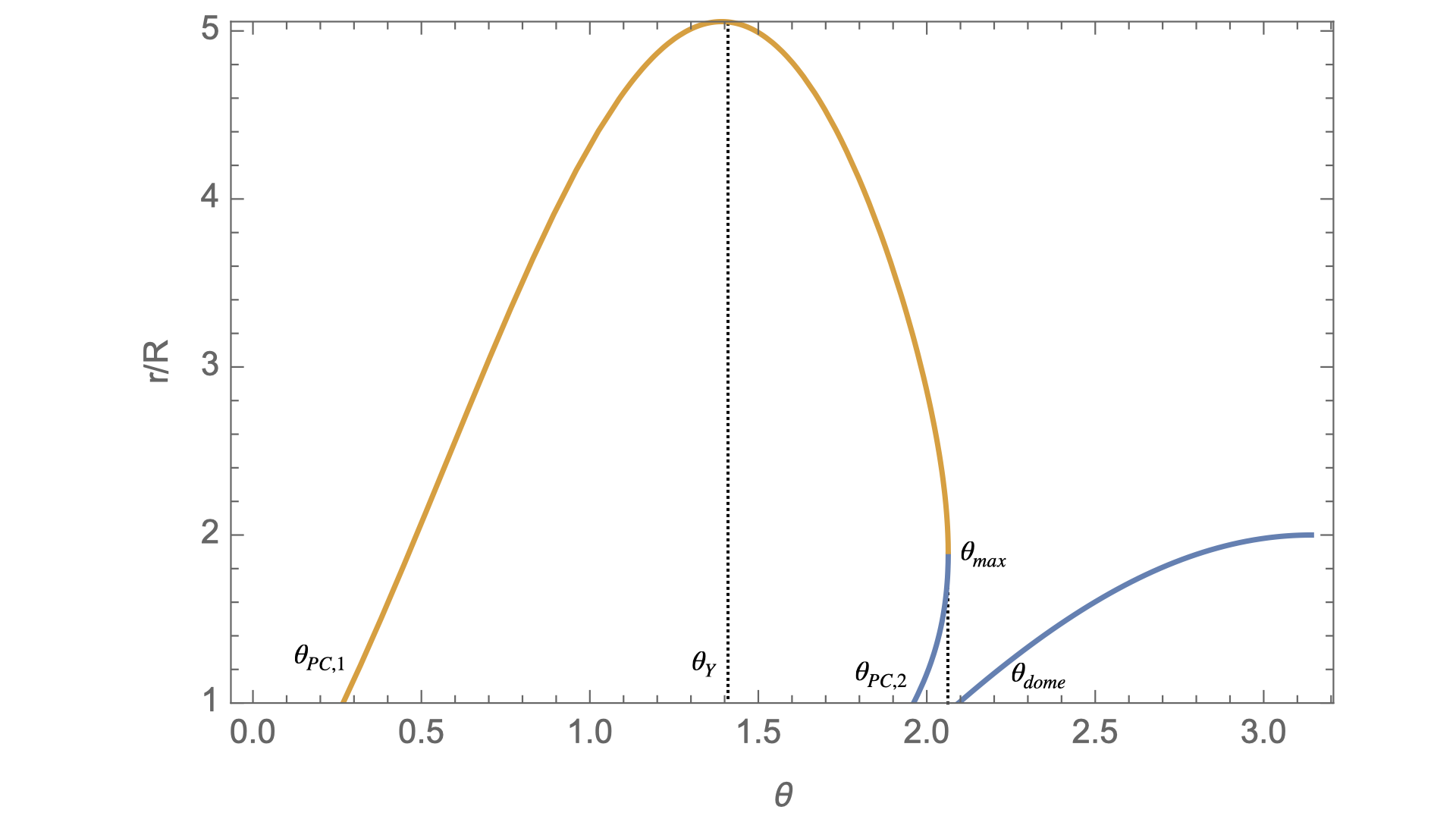
Figure 23: Last closed field lines and the southern dome for the dipole-plus-quadrupole configuration with $\mu_{q}=2$.

We then study three different configurations: (i) dipole; (ii) mixed dipole-quadrupole; (iii) mixed dipole-octuple. The relative strength of the higher multipoles is parameterized by $\mu_{q}$ and $\mu_{o}$. In what follows we use $\mu_{q}=2$ and $\mu_{o}=3$ - in these cases the higher order multipoles introduce non-trivial corrections to the surface fields, if compared with dipolar (e.g. , in case of dipole-quadrupole configuration, a “dome” appears near the south pole), see Figs. 2 and 23.

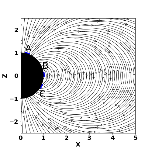
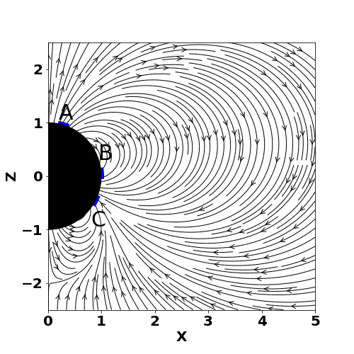
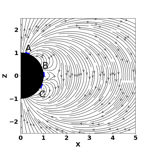
Figure 2: Initial poloidal field lines for superposition of dipole, dipole plus quadrupole, and dipole plus octupole (left to right) for $\mu_{q}=2$ and $\mu_{o}=3$, see Eq. (12). Shearing region A,B, and C are at $20^{\circ}$, $90^{\circ}$, and $120^{\circ}$ respectively from the z-axis. Here and below scales are normalized to neutron star radius.

3.2 Prescriptions for foot-point shear

The second important ingredient is the location of the shear. The imposed shear on magnetic foot-points is confined to a small band, to be located at various latitudes and of latitudinal extent. The shearing is applied at the inner boundary of our simulation, the radius of the star.

When the two foot-points of the sheared arcade are well separated, we employ symmetric shear, moving azimuthally only one set of footprints (This is nearly equivalent to anti-symmetric shear, when the two footprints are moved in the opposite direction, given the overall spin of the star). The symmetric shear fails to create an expanding flux tube for the case of equatorial shear - in that case symmetric shear moves both footprints in the same direction, so that the global magnetosphere can remain stationary (Lyutikov & Sharma, 2022). To induce explosion for the equatorial shear we apply antisymmetric prescription, Eq. 15.

We employ several prescriptions for symmetric shear. First, we follow the discussion in section 3 of Antiochos et al. (1999). In that case the angular velocity of the foot-points $\omega_{s}$ is (see Fig. 3)

$$\omega_{s}(\theta)=\left\{\begin{array}[]{ll}\omega_{max}g(\theta),&\text{ for }\theta_{band}-\Theta\leq\theta\leq\theta_{band}\\ 0,&\text{ otherwise }\end{array}\right.$$ (13)

Here, $\omega_{max}$ is the maximum value of applied shear, and function $g(\theta)$,

$$g(\theta)=C\left(\psi^{2}-\Theta^{2}\right)^{2}\sin\psi\mbox{}$$

$$\psi=\theta_{band}-\theta,$$ (14)

defines the latitudinal extent of the shear region, and $\theta_{band}$ is the polar angle around which shearing is applied. $C$ is a normalization constant introduced to ensure that max$|g(\theta)|=1$ and $\Theta=\pi/15$ is the assumed latitudinal extent of the shear layer.

We can also construct expression for anti-symmetric shearing as below:

$$\omega_{s}(\theta)=\left\{\begin{array}[]{ll}\omega_{max}g(\theta),&\text{ for }\theta_{band}-\Theta\leq\theta\leq\theta_{band}+\Theta\\ 0,&\text{ otherwise }\end{array}\right.$$ (15)

Since for the rotating case, we are mostly interested in ratio of shear velocity to the stars rotation velocity, we rearrange Eq. 13, to get

$$\frac{\omega_{s}}{\Omega_{\star}}=\left\{\begin{array}[]{ll}\xi g(\theta),&\text{ for }\theta_{band}-\Theta\leq\theta\leq\theta_{band}\\ 0,&\text{ otherwise }\end{array}\right.$$ (16)

Where $\xi={\omega_{max}}/{\Omega_{\star}}$.

The shear profile for both symmetric and anti-symmetric case, as the function of $\theta$ is plotted in Fig. 3 for three different location of shearing band.

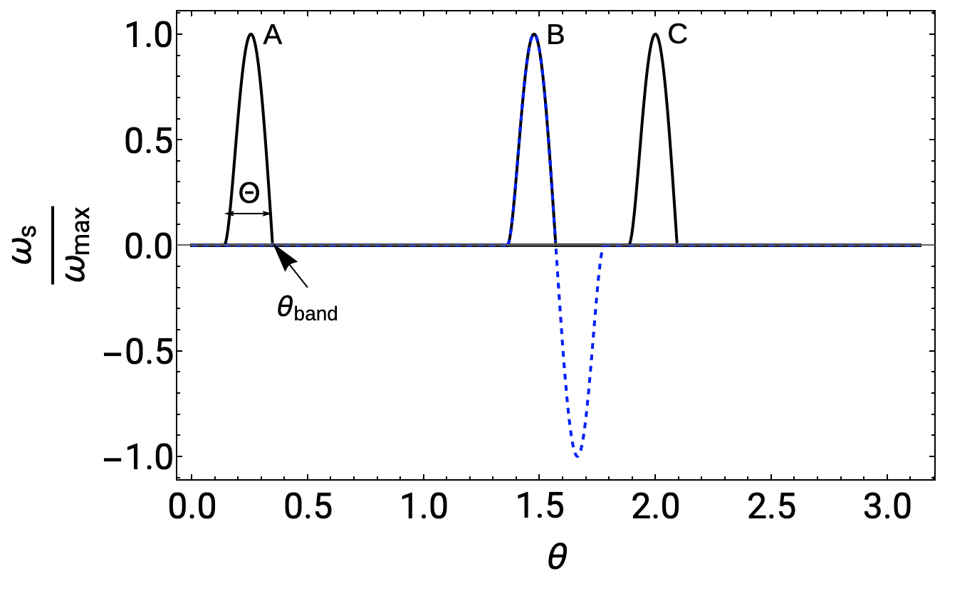
Figure 3: Normalized shear velocity ($\omega_{s}/\omega_{max}$) as a function of co-altitude $\theta$ (see Eq. 13,15). Solid black curves shows shear profile for symmetric mode at three different regions (A,B,C) whereas blue dashed line represent the shear profile for anti-symmetric mode near the equator (region B).

4 Coronal mass ejections deep inside magnetospheres.

4.1 Sheared non-rotating magnetospheres

We start this work by probing static non-rotating configurations with shearing introduced at different locations. The main justification is the limited dynamic range of simulations of the rotating magnetospheres, §5. Our typical light cylinder radius is only 5 stellar radii, while in case of magnetar the expected ratio is in the tens of thousands (for $\sim 1$ second period).

As a key new ingredient, we probe the effect of various magnetic field topologies by adding contributions from other multipoles. We achieved this by superimposing quadrupole and octupole field on star’s dipolar field (see §3.1). Since we are mostly interested in the plasmoid ejections, we chose relatively high shearing rate to ensure the magnetosphere enters into a non-equilibrium dynamic states (Parfrey et al., 2013; Mikic & Linker, 1994). For this and the subsequent simulations, the maximum shearing rate $\omega_{max}$ was chosen as $0.1$ (so that the light cylinder corresponding to the shearing motion is at 10 stellar radii.)

The shearing of foot-points starts immediately at beginning of simulations $t=0$, causing the field lines to twist. The subsequent evolution of the system is visualized in Fig. (4), where we plot toroidal current density $J_{\phi}$ for combination of different shearing altitude and magnetic field topology. To demonstrate the importance of location of foot-point shearing, we consider three different shearing regions: near the poles (region A), at equator (region B), and at $\sim 120^{\circ}$ from the poles (region C).

(a)Region A: $20^{\circ}$

(b)Region B: $90^{\circ}$

(c)Region C: $120^{\circ}$

Dipole

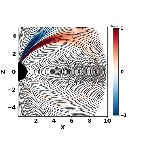
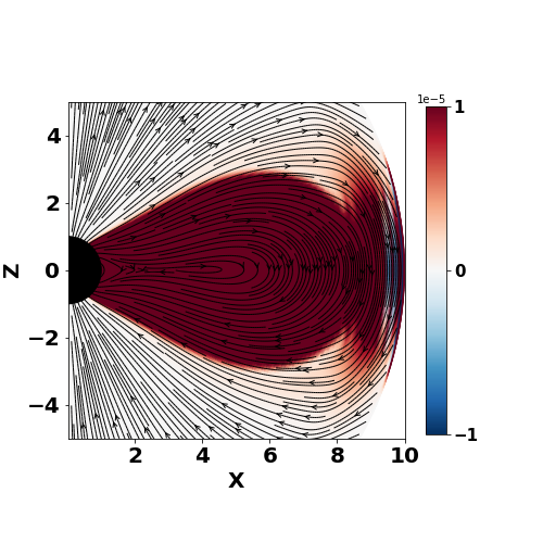
Dipole+Quadrupole

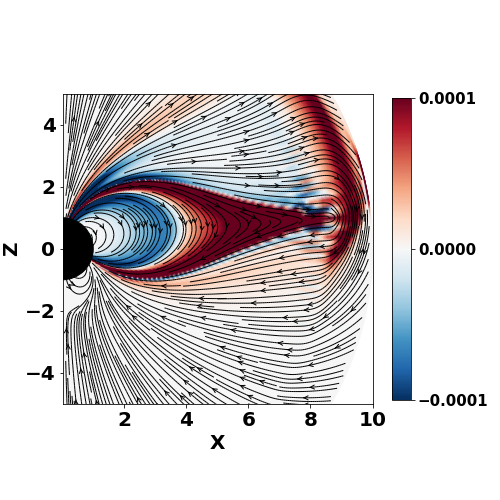
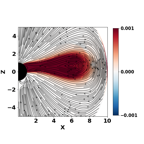
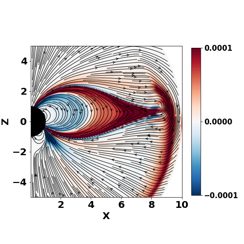
Dipole+Octupole

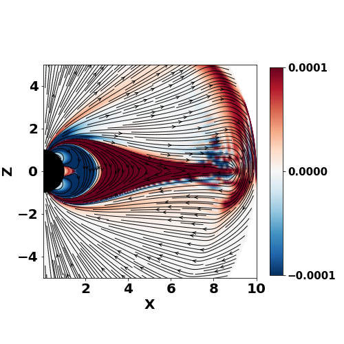
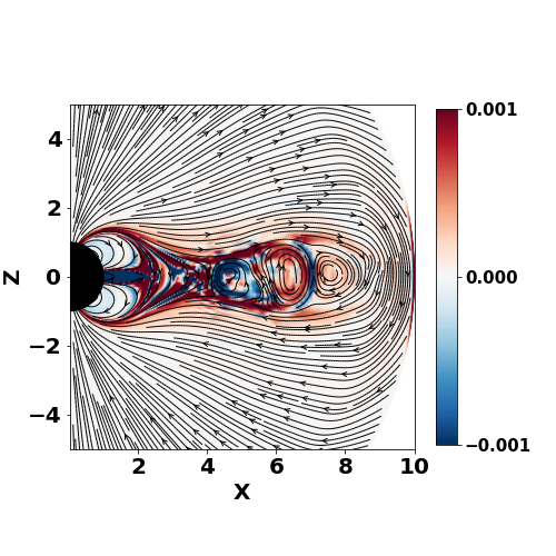
Figure 4: Toroidal current density$(J_{\phi})$ for non-rotating configurations shear at various altitudes ($20^{\circ}$, $90^{\circ}$, and $120^{\circ}$ from left to right). Shearing rate is $\omega_{max}$ =0.1. In all cases, when shearing is done close to the north pole (region A, left column), no major ejection events are observed. When shearing near the equator (region B, middle column), in all cases we observe powerful ejections. When shearing is done at region C (right column) whether or not ejections are observed depend on the magnetic field topology. Red boxes are drawn around configurations where a clear expulsion of plasmoids is observed.

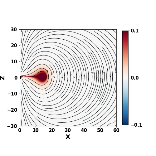
(a)

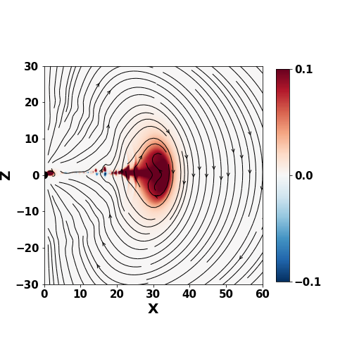
(b)

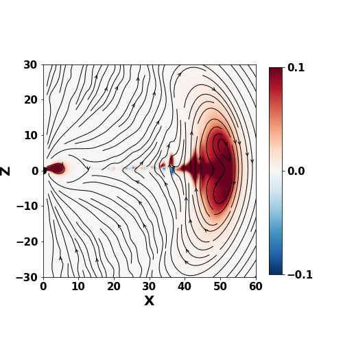
(c)

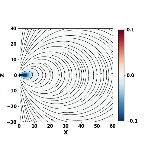
(d)

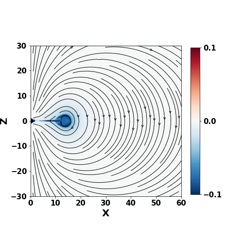
(e)

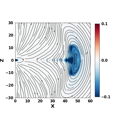
(f)

Figure 5: Time evolution for non-rotating dipole+ quadrupole sheared at point B (top panel), and dipole sheared anti-symmetrically at point B (bottom panel). Color is toroidal magnetic field $r\sin(\theta)B_{\phi}$ (this applies other figures unless stated otherwise), streamlines are poloidal fields. Shearing starts at beginning of the simulation.

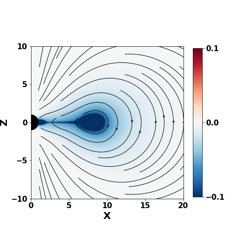
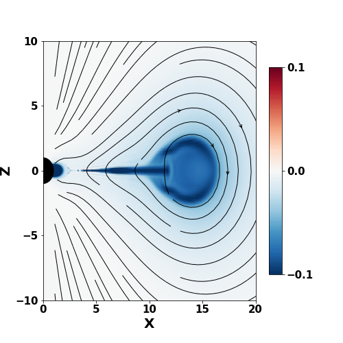
Figure 6: Detonating CME within the magnetosphere. Right panel: zoomed-in version of Fig. 5e: notice the edge-enhances structure of the detonating CME, cf.  Fig 1. As discussed by Barkov et al. (2022), detonating magnetic structures are concentrated near the surface. Left panel: we show the system approximately a third of a period before the detonation.

No ejections were seen when shearing region is located near the poles (Region A) for all three initial magnetic field topology. As observed in Fig. 4 left panel, there isn’t substantial poloidal expansion and the system attains a quasi-equilibrium state where most of the field lines remain closed.

For the case equatorial shearing (region B), we see major explosive events for superposition of dipole and quadrupole/octupole topologies. We attribute this to the significant opening of the closed lines. While the ejection is evident for the case of dipole and octupole superposition, we show the final inflated state for remaining two configurations: the structure breaks away and exits the simulation box at the next time step. This equatorial expansion is consistent with previous simulations by other authors (Parfrey et al., 2013; Mikic & Linker, 1994). As argued in above mentioned works, field line opening causes the formation of a current sheet and the subsequent reconnection of field lines triggers ejection of magnetic energy in the form of plasmoids.

The ejections profile while shearing region C, however depends on the magnetic topology, as depicted in Fig. 4 right panel. Unlike in the case of dipole and dipole+octupole magnetosphere, the field lines for dipole+quadrupole topology are only partially open and the system achieves a quasi-equilibrium state. In Fig. 4 we highlight those cases where the system explodes and ejects plasmoids with a red box.

We further show the large scale time evolution of two selected configuration : dipole+quadrupole, and dipole sheared anti-symmetrically in Fig. 5. We see ejection events in both scenarios, albeit at different time. In Fig. 6, we zoom in on Fig. 5e to highlight the structure of the exploded shell - most of the energy/magnetic field  is concentrated near the surface of a detonating flux tube as discussed/ simulated by Barkov et al. (2022).

5 Coronal mass ejections by rotating magnetospheres (slow shear)

5.1 Results: magnetospheric dynamics for slow shear

Next we proceed to the main topic of this paper: dynamics of Coronal Mass Ejections (CMEs) in relativistic rotating magnetospheres with sheared foot points. For slow shear we set $\omega_{max}=0.1$, which corresponds to $\xi=0.5$ (maximal shearing rate is half the spin). The shearing of the stellar surface begins after one rotational time period, to ensure that our initial un-sheared system is in an equilibrium state.

We start with basic case of dipolar magnetosphere sheared at the equator with anti-symmetric shearing profile (15), Fig. 7. We introduce magnetic foot-point shearing to rotating neutron stars. One can clearly observe the opening of field line and ejection of a CME. After the CME the closed part of the magnetosphere is smaller, with the current sheet showing plasmoid instability. The final configuration has non-zero twist on closed field lines.

The behavior matches the expectations: the closed field lines become partially or even fully opened in response to finite foot-point shearing due to additional magnetic pressure from the toroidal component of the magnetic field (Wolfson & Low, 1992). The opened field lines subsequently causes the expulsion of magnetic energy in the form of Coronal Mass Ejections. The post-CME relaxation is a new effect: formation of smaller closed magnetosphere, with plasmoid-mediated current sheet deep inside the light cylinder, and a slow, reconnection-mediated relaxation to a new equilibrium with twisted field lines.

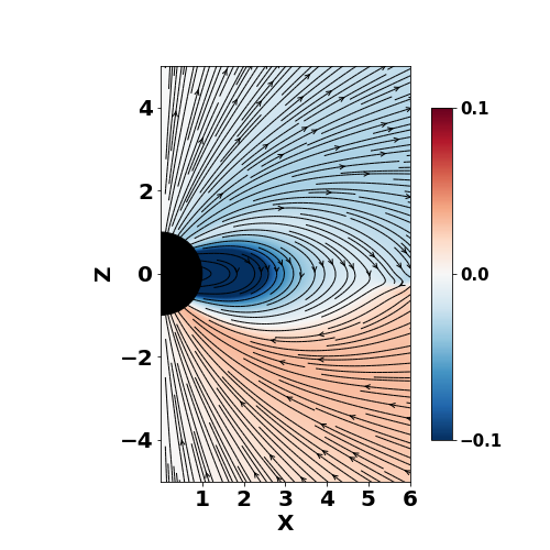
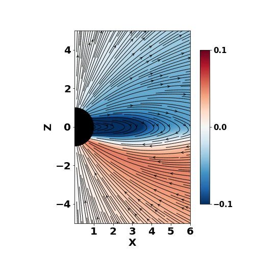
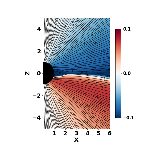
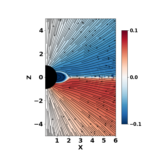
Figure 7: Time evolution for rotating dipole configuration sheared anti-symmetrically at point B (equatorial), slow shear. Snapshots are taken at $t=\{0.95,3.2,5.4,6.4,7.0,7.3\}$. Shearing starts at $t=1$ (after one rotation period). One can clearly observe the opening of field line and ejection of a CME. After the CME is ejected the closed part of the magnetosphere is smaller, with the current sheet showing plasmoid instability. The final configuration has non-zero twist on closed field lines - compare first and last panels. See also Fig. 12 for the large scale dynamics.

Next we show time evolution of sheared dipole and quadrupole system for equatorial shearing in Fig. 8, left column. The opening of field lines and subsequent ejection of CME is clearly evident. In Fig. 8 we compare the dynamics the same configuration (dipole + quadrupole configuration sheared at point B), between rotating and non-rotating cases. We clearly see that it is much easier to break out from the rotating magnetosphere. This is expected, since in the rotating case the breakout occurs when the top of the inflated loop reaches the light cylinder. Fig. 8 also demonstrates that though our dynamic range is not very large (light cylinder at only five stellar radii), we do correctly capture the dynamics of the inflated flux tube within the magnetosphere.

In Fig. 8 we compare the dynamics the same configuration (dipole + quadrupole configuration sheared at point B), between rotating and non-rotating cases. We clearly see that it is much easier to break out from the rotating magnetosphere. This is expected, since in the rotating case the breakout occurs when the top of the inflated loop reaches the light cylinder. Fig. 8 also demonstrates that though our dynamic range is not very large (light cylinder at only five stellar radii), we do correctly capture the dynamics of the inflated flux tube within the magnetosphere.

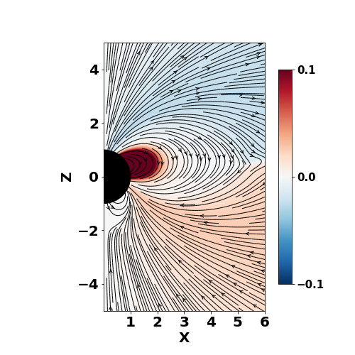
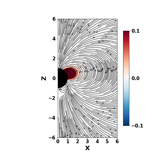
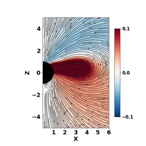
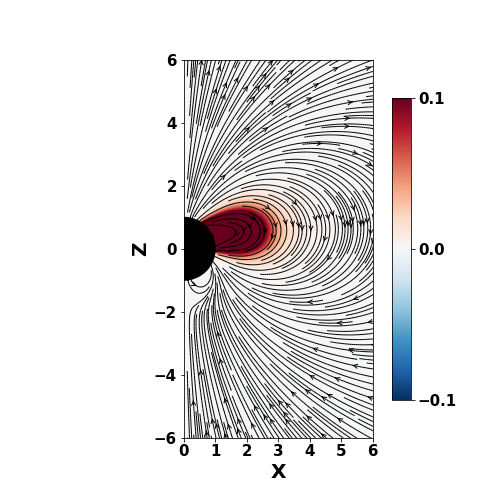
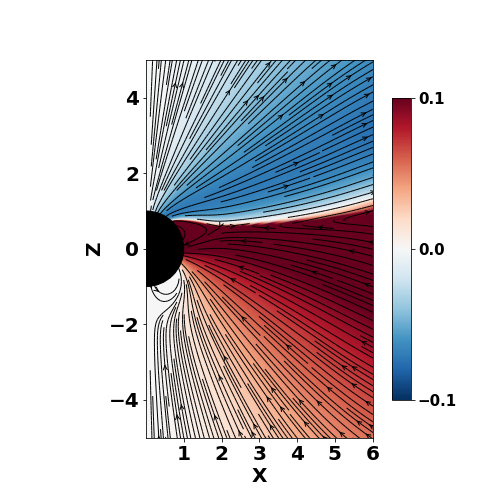
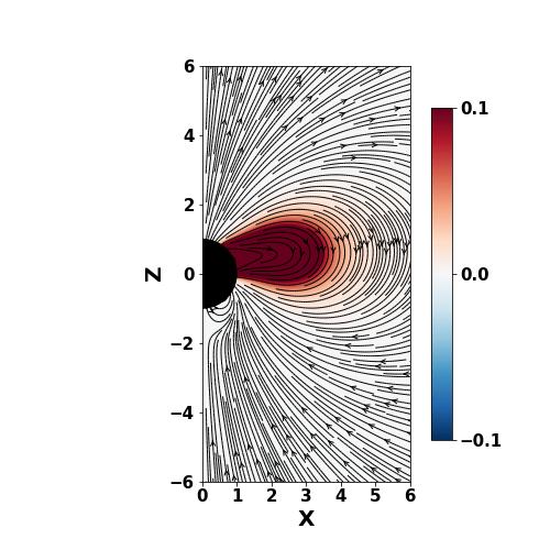
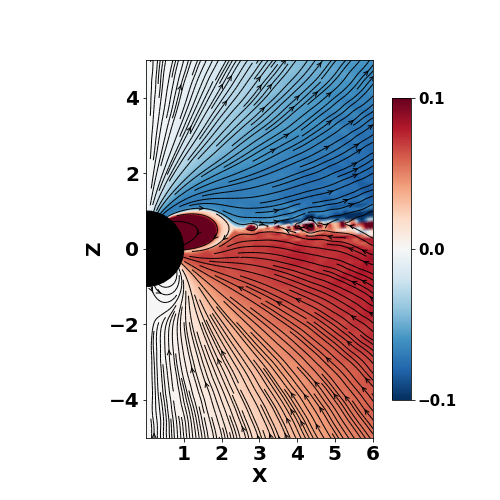
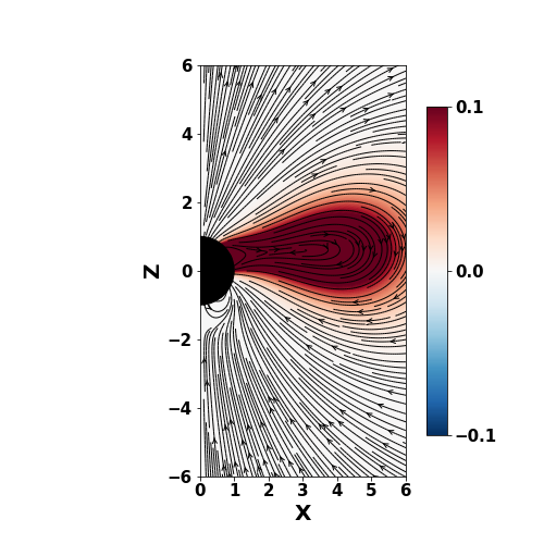
Figure 8: Dipole + quadrupole configuration sheared at point B (equatorial), slow shear. Left column: rotating case, right column: non-rotating case (snapshots are taken at same time, as measured from the start of the shearing.). One clearly sees the influence of the light cylinder on the development of the CME. This demonstrates that the light cylinder makes it “easier” for the CME to break out.

Finally, in Fig. 9 we discuss all three magnetic configuration sheared at various locations. The top panel shows systems with only dipole field. No ejections were observed when shear is applied near the polar area (region A) and the system remained in quasi-equilibrium state. Similar to what we observed in previous section for non-rotating system, this observation will hold true even for more complicated magnetic topologies. We also don’t observe ejections while shearing near equator (region B). This is consequence of the fact that our shearing profile is symmetrical i.e. for the equatorial case, the shearing is confined to one hemisphere.

In middle panel we consider rotating star system with superposition of dipole and quadrupole field, we find that powerful ejection events are observed when shearing between $\sim 30^{\circ}$ and $100^{\circ}$. This is consistent with our hypothesis that strong ejections are observed while shearing region with closed field lines (bigger loop in Fig. 10). We demonstrate our results by plotting the toroidal current at three different locations : near the poles (region A), at equator (region B), and at $\sim 120^{\circ}$ from the poles (region C). In the bottom panel we consider simulations with superposition of dipole and octupole field. Powerful plasmoid ejection events are observed once the shearing region is away from the polar region .

Based on above results, we can safely conclude that the effects of shearing highly dependent on how far the field lines extent. Shearing closed field lines leads to powerful ejections whereas if the shearing region is located in an area where field lines have started opening out, no or weak pulsating ejections are observed. Following the discussion in § 4.1, we highlight those cases where the explosion can be observed with a red box. In Table 2 we summarize our results for rotating sheared configurations (see also §6.4 for a related case of fast shear).

(a)Region A: $20^{\circ}$

(b)Region B: $90^{\circ}$

(c)Region C: $120^{\circ}$

Dipole

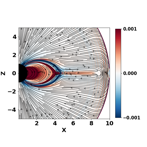
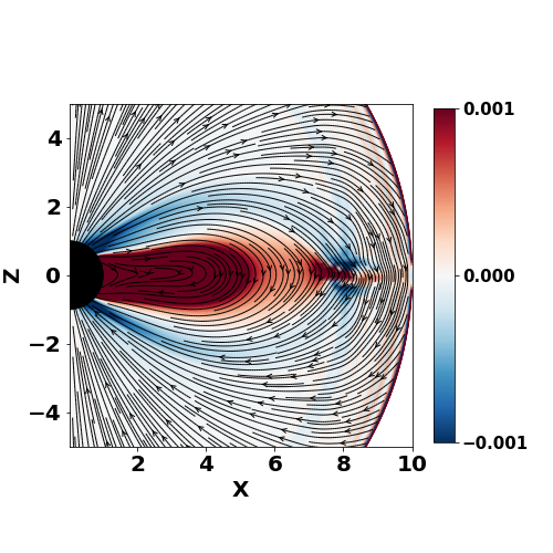
Dipole+Quadrupole

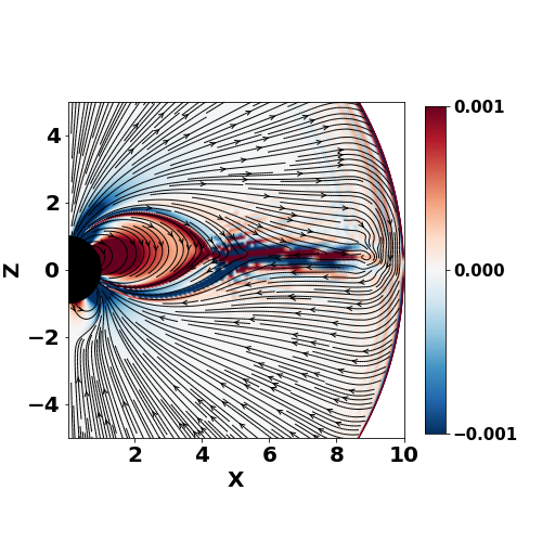
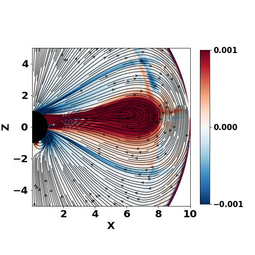
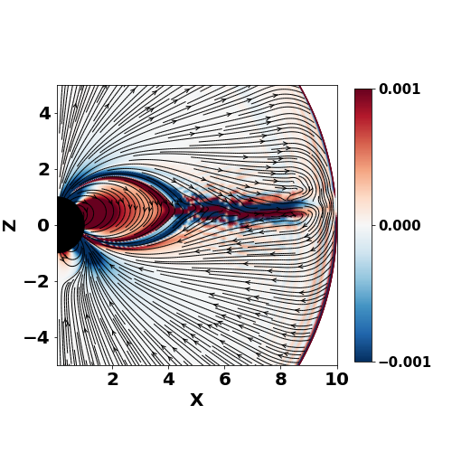
Dipole+Octupole

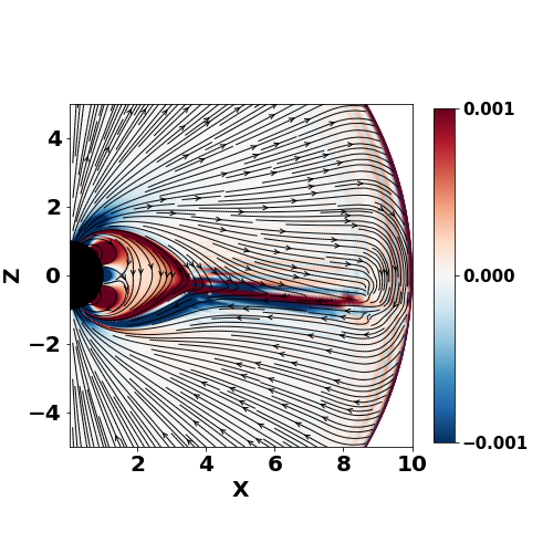
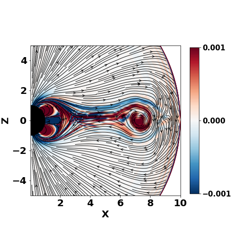
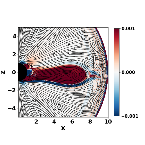
Figure 9: Toroidal current density $J_{\phi}$ for rotating and sheared configurations. Overall angular velocity of the star is $\Omega=0.2$ (so that the light cylinder is at $x=5$), normalized shear parameter $\xi=0.5$ (so that maximal shearing angular velocity is $\omega_{max}=0.1$), symmetric shear (so that all footpoints are moved in the same azimuthal direction) In all cases, when shearing is done close to the north pole (region A, left column), no major ejection events are observed. When shearing near the equator (region B, middle column), in all cases we observe powerful ejections. When shearing is done at region C (right column) whether or not ejections are observed depend on the magnetic field topology: in the Dipole+Quadrupole case (second row, right column) no powerful ejections are observed. Red boxes are drawn around configurations where a clear expulsion of plasmoids is observed.

Field Topology	Shearing Region
	Region A	Region B	Region C
Dipole	Weak pulsating eruptions [Fig. 9(a),Top Panel]	Weak pulsating eruptions [Fig.9(b),Top Panel)]	Powerful ejections [Fig.9(c),Top Panel)]
Dipole+Quadrupole	Weak pulsating eruptions [Fig. 9(a), Middle Panel]	Few but powerful [Fig. 9(b),Middle Panel]	Weak pulsating eruptions [Fig. 9(c),Middle Panel]
Dipole+octupole	Weak pulsating eruptions [Fig. 9(a),Bottom Panel]	Frequent and powerful [Fig. 9(b),Bottom Panel]	Frequent and powerful [Fig. 9(c),Bottom Panel]

Table 2: Table summarizing results from simulations when the magnetic field lines are sheared for rotating stars, following the prescription in Antiochos et al. (1999).

5.2 Conclusion 1: three important ingredients for generation of CME: global magnetospheric structure, location of foot-point shear, and rotation

Different magnetic field configurations are required for CME initiations by different models (Li & Luhmann, 2005). The Break-out model proposed by (Antiochos et al., 1999) has a multi-flux topology with four distinct flux systems. The shearing of the central arcade (which straddles the equator) and the subsequent reconnection of the sheared magnetic arcade with the overlying un-sheared field leads to build up of large energy excess in closed sheared field lines, to power CME.

Another similar model was proposed by Mikic & Linker (1994), where the trigger for plasmoid ejections is the introduction of resistivity in the plasma when the shearing is turned off. The introduction of resistivity causes the magnetic field lines to reconnect in the current and the subsequent formation and ejection of plasmoid islands. In absence of plasma resistivity no eruption occurs, field lines becomes fully opened and the system remains in equilibrium.

The major difference between this work and model by Antiochos et al. (1999) is the inclusion of the rotation of the star. The rotation of star, which in turn leads to formation of light cylinder, removes the need for magnetic reconnection. The flux tube opens up to infinity approximately when the top point reaches the light cylinder.

We find a relatively simple picture of shear-generated explosion: the location of the shear for a given global magnetospheric structure determines the presence or absence of strong ejection events. Qualitatively, we show the results for dipole+quadrupole configuration in Fig. 10.

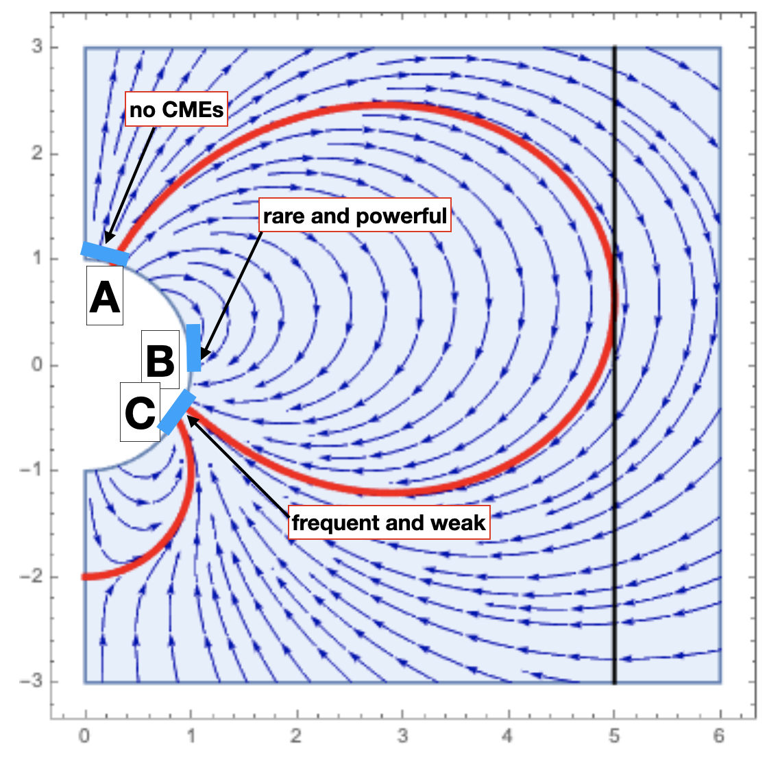
Figure 10: Qualitative description of flare dynamics depending on the location of the shear (dipole-quadrupole case). Vertical line at $5$ is a light cylinder.

5.3 Large scale dynamics of ejected CMEs in the wind, and conclusion 2

Previously, in §5.1 we discussed generation of a CME within the magnetar’s magnetospheres. Next we study the large scale dynamics of the resulting CME. We stat with large scale simulation showing time evolution of a sheared dipole+quadrupole configuration, see Fig. 11. Here we set the outer boundary far away from the light cylinder.

In Figs. 12 and 13 we plot a large scale snapshot for the two cases of dipolar fields sheared anti-symmetrically and dipole plus quadrupole configuration sheared at point B.

Recall that shearing results in the generation of topologically disconnected flux tube, a CME. In Figs. 12 and 13 an ejected CME is clearly identified in the left panels around $x\approx 25$. At the same time, the CME are barely seen in the Lorentz factor/ radial momentum plots (center and left panels): topologically disconnected CME is frozen into the wind and propagates with the local Lorentz factor of the wind.

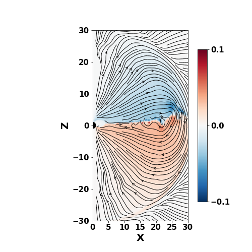
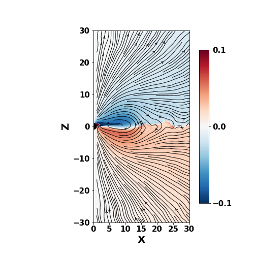
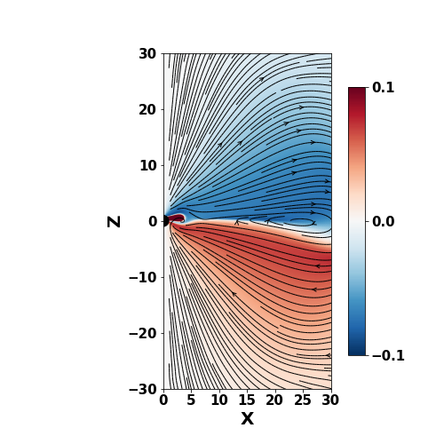
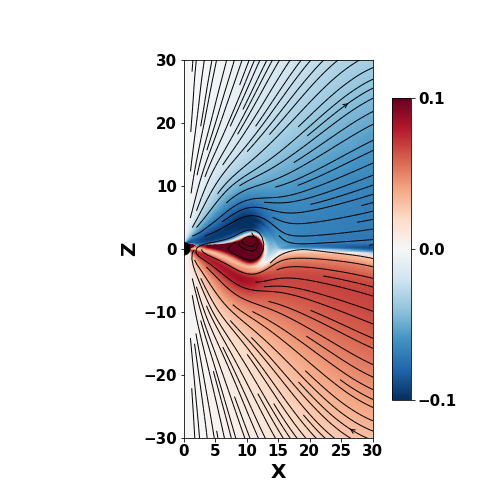
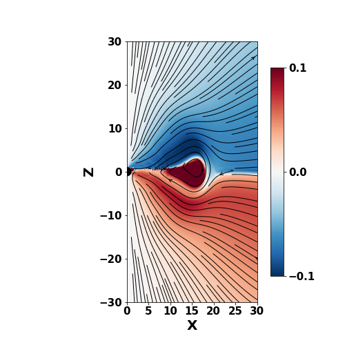
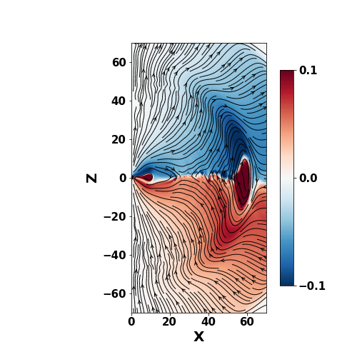
Figure 11: Rotating dipole + quadrupole configuration sheared at point B (equatorial), slow shear on large scale. The snapshots are taken at $t={0.99,2.4,3.2,3.6,3.8,5.3}$ of the rotational period of the star. Shearing is introduced after one rotation. One can clearly observe the opening of field line and ejection of a CME. After the CME the closed part of the magnetosphere is smaller, with the current sheet showing plasmoid instability. The final configuration has non-zero twist on closed field lines.

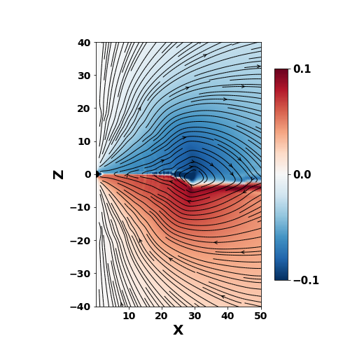
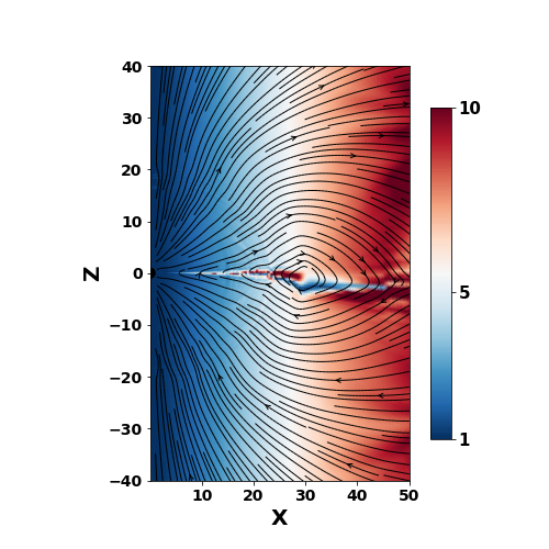
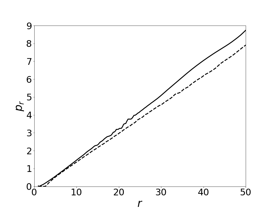
Figure 12: Similar to Fig. 7 (dipolar field sheared anti-symmetrically at region B) but on large scales. Plotted are values of $r\sin\theta B_{\phi}$ (left panel), Lorentz factor (middle panel) and radial momentum $p_{(}r)$ as a function of radial distance r at a zenith angle of $60^{\circ}$ from the pole for the above configuration (solid) and for unsheared rotating dipolar configuration (dashed). The snapshots are taken at t= 7.8. As observed from middle and left plot there is minimal effect of the ejection on the Lorentz factor $\Gamma$.

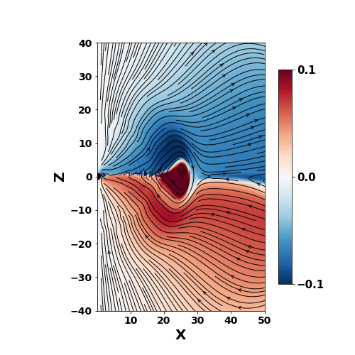
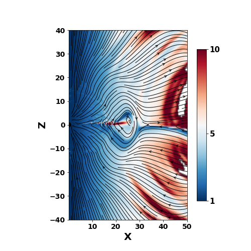
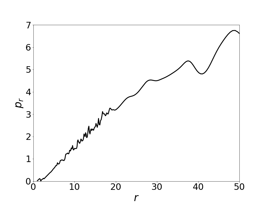
Figure 13: Similar to Fig. 11 (dipole + quadrupole configuration sheared at point B) but here we show Lorentz factor $\Gamma$ and radial momentum $p_{r}$ as a function of radial distance r at a zenith angle of $60^{\circ}$ from the pole along with scaled toroidal magnetic field at t= 4.1. As observed from middle and left plot there is minimal effect of the ejection on the Lorentz factor $\Gamma$.

Overall, our numerical results are in excellent agreement with analytics (Lyutikov, 2022), see Fig. 1.

6 Glitched Magnetosphere (fast shear)

6.1 Magnetar’s CMEs in the Star Quake paradigm

In a complementary approach, which can be supported by a fully analytical model, we consider a model of propagation of the force-free electromagnetic pulse generated by a sudden local spin-up of a neutron star, a “Glitched Magnetosphere”. This type of dynamics mimics the starquake model of Thompson & Duncan (1995); Yuan et al. (2020)

6.2 Locally glitched Michel’s magnetosphere: analytical approach

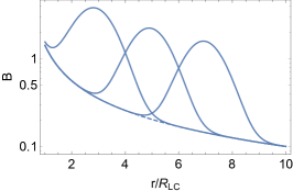
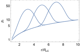
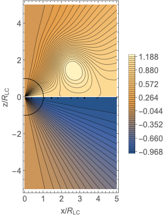
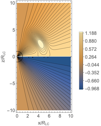
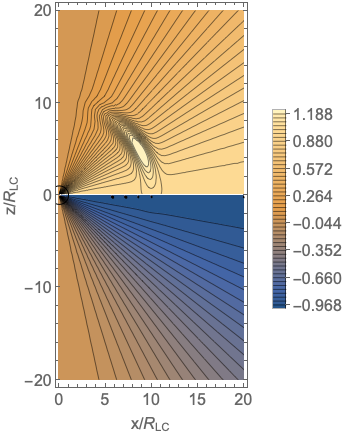
Figure 14: Top row. Left Panel: Structure of the magnetic field in the equatorial plane of an electromagnetic Gaussian pulse with amplitude $10$ times the average propagating through Michel’s wind. The peak of the pulse is at $r/R_{LC}=3$. The light cylinder  is at $\sqrt{x^{2}+y^{2}}=1$. Color scheme corresponds to $\ln B/B_{M}$, where $B_{M}$ is the local value of the magnetic field for Michel’s solution. Center Panel: plot of $B$ showing EM pulse propagating with the wind for times $t=3,5,7$ (in units of $R_{LC}/c$); dashed line is the Michels’ solution. Right panel: plot of $p_{r}(r)$. The pulse propagates with the flow with constant relative amplitude, without experiencing any distortions. Bottom row: value of $r\sin\theta B_{\phi}$

Effects of “glitch in spin” on the structure of the wind can actually be considered analytically and non-perturbatively for the case of Michel (1973) magnetospheres  and the preceding wind:

$$\mathbf{B}=B_{0}\left\{\frac{r_{0}^{2}}{r^{2}},0,-\frac{r_{0}^{2}\Omega\sin(\theta)}{r}\right\}\mbox{}$$

$$\mathbf{v}=\left\{\frac{r^{2}\Omega^{2}\sin(\theta)^{2}}{1+r^{2}\Omega^{2}\sin(\theta)^{2}},0,\frac{r\Omega\sin(\theta)}{1+r^{2}\Omega^{2}\sin(\theta)^{2}}\right\}\mbox{}$$

$$\mathbf{\Gamma}=\sqrt{1+r^{2}\Omega^{2}\sin(\theta)^{2}}\mbox{}$$

$$\mathbf{p}=\left\{\frac{r^{2}\Omega^{2}\sin(\theta)^{2}}{\sqrt{1+r^{2}\Omega^{2}\sin(\theta)^{2}}},0,\frac{r\Omega\sin(\theta)}{\sqrt{1+r^{2}\Omega^{2}\sin(\theta)^{2}}}\right\}$$ (17)

$B_{0}$ is the the fiducial magnetic field magnitude at the light cylinder ($r_{0}$) and we set $c=1$. Realistic dipolar magnetospheres do evolve asymptotically to the Michel (1973) solution (Bogovalov, 1999; Contopoulos et al., 1999; Komissarov, 2006).

One can generalize Michel’s solution for any arbitrary time- and angle dependent rotation $\Omega=\Omega[r-t]g(\theta)$ Lyutikov (2011) (see also Gralla & Jacobson, 2014). (The solution can also be generalized to Schwarzschild metric using the Eddington-Finkelstein coordinates Lyutikov, 2011). This glitch in spin time-dependent nonlinear solution (nonlinear both in a sense that the current is a non-linear function of the magnetic flux function, and that the perturbation can be of large amplitude) preserves both the radial and $\theta$ force balance. Qualitatively, ”a glitch” in the angular rotation velocity $\Omega$ mimics a symmetric shearing motion of a patch of field lines (we remind: “symmetric” means overall motion in one direction along $\phi$). Approximation of Michel (1973) magnetospheres  misses the magnetospheric dynamics, but it capture the wind dynamics.

In Fig. 14 we show the evolution of single Alfvén pulse using $g(\theta)=\sin^{10}(\theta+\pi/4)$ and $\Omega=1+e^{-(r-t)^{2}}$. To complement the analytical work, we show the complete evolution of a pulse via numerical simulation in § 6.3

A pulse of shearing Alfvén waves with $\Omega[r-t]g(\theta)$ propagates with radial 4-momentum

$$p_{r}=\frac{r^{2}\sin^{2}\theta\Omega^{2}[r-t]g(\theta)^{2}}{\sqrt{1+r^{2}\sin^{2}\theta\Omega^{2}[r-t]g(\theta)^{2}}}$$ (18)

which is larger than that of the wind for $\Omega[r-t]g(\theta)\geq\Omega_{0}$, the constant value. Higher radial momentum (than that of the background flow) does not mean that plasma is swept-up: it’s just an EM pulse propagating through the accelerating wind.

6.3 Locally glitched magnetosphere: simulations with PHAEDRA

In a numerical implementation we limit ourselves to just dipolar magnetospheres. We use glitch parametrization as

$$\Omega=\Omega_{0}\left(1+g(\theta)f(t)\frac{\delta\Omega}{\Omega_{0}}\right)$$ (19)

Several types of shearing were implemented: (i) overall glitch $g(\theta)=$ constant (so in this case the glitch is actually global); (ii) symmetric $g(\theta)=\sin^{10}(\theta+\pi/4)$; (iii) and anti-symmetric near equator $g(\theta)=\sin^{3}(\theta)\cos(\theta)$. The extra rotation within the shearing band is fast ${\delta\Omega}/{\Omega_{0}}=5$.

Time dependence of the glitch is

$$f(t)=\sin[\pi(t-t_{on})/\tau]\mbox{}$$

$$t_{on}=P\,\mbox{(one period)}\mbox{}$$

$$\tau=P/10\mbox{}$$

$$t_{off}=t_{on}+\tau$$ (20)

so that the glitch is implemented after one rotation for one tenth of the with maximum rate reached at $t=t_{on}+\tau/2$. Thus a total shearing angle is $\Delta\phi=\pi$. Note that the shearing expression $g(\theta)$ used in this section is somewhat different from the one used for slow shearing.

6.3.1 Overall glitch

We first consider the case of constant $g(\theta)$ i.e. the entire magnetosphere is glitched instead of a narrow band. We demonstrate our findings in Fig. 15 where we plot $r\sin(\theta)B_{\phi}$ at different time steps.

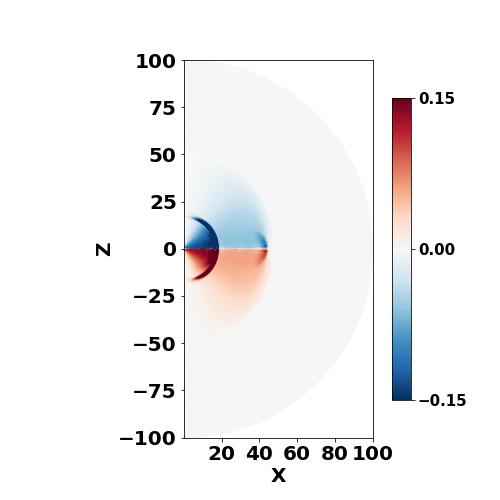
(a)

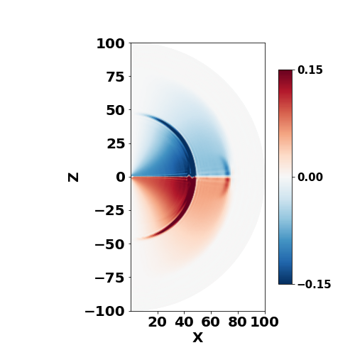
(b)

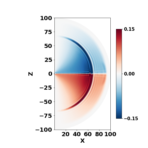
(c)

Figure 15: Global glitch with $g(\theta)=const$, large scale view. Snapshots of $r\sin(\theta)B_{\phi}$ are taken at $t=1.6,2.5,3.2$ rotation periods. A glitch produced a global Alfvén wave propagating through the wind.

6.3.2 Narrow symmetric glitch at $\theta=\pi/4$

Results of simulation are presented in Fig. 16 (zooming in close to the star), and bottom row of Fig. 17 (long time scale evolution). In Fig. 16 we show zoomed-in plots for $r\sin(\theta)B_{\phi}$ superimposed on poloidal field lines for symmetric shear: narrow band near $\theta=\pi/4$ is suddenly moved with angular velocity 5 times the spin. We start with unperturbed magnetosphere (Fig. 16a), one period after the star of overall rotation. Then, shear is introduced, Fig. 16b - blue region near the star at $\theta\approx\pi/4$. The resulting shear Alfvén wave breaks out from the magnetosphere, Fig. 16c. The magnetosphere recovers: bottom row. A new Y-point is formed close to the star (compare locations of the Y-points before the shear is introduced in Fig. 16a and right after break-away, Fig. 16d). Outside of the newly formed Y-point reconnection layer forms. It is subjected to plasmoid instability Fig. 16d-16e. Eventually, the magnetosphere recovers, to approximately the same location of the Y-point, Fig. 16f. Notice that the newly formed magnetosphere is twisted: there is non-zero toroidal magnetic field on closed field lines.

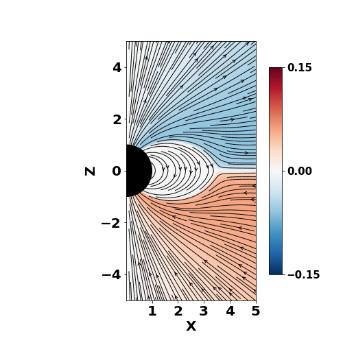
(a)

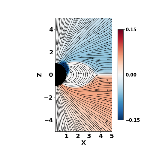
(b)

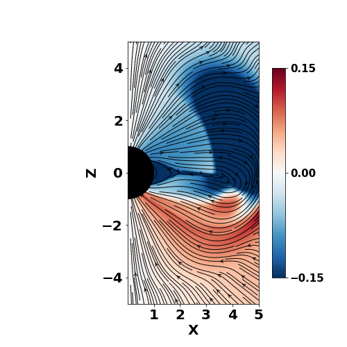
(c)

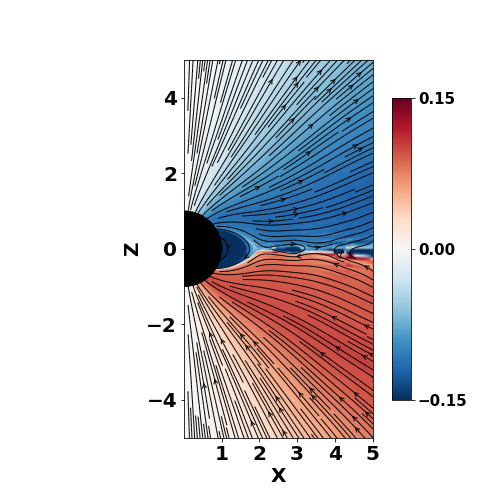
(d)

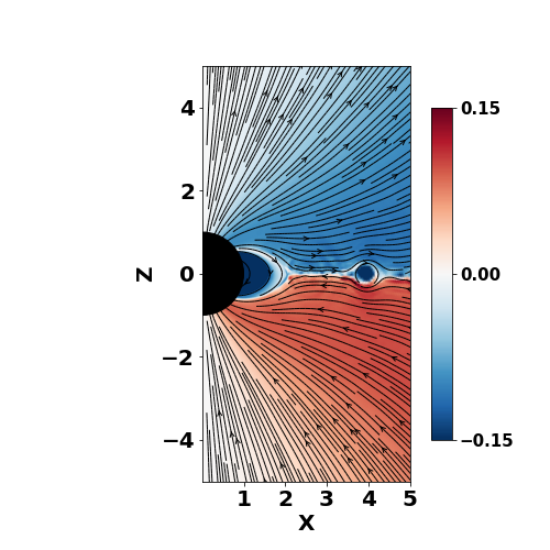
(e)

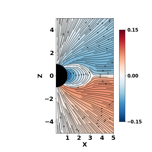
(f)

Figure 16: Fast glitch near $\theta=\pi/4$, $g(\theta)=\sin^{10}(\theta+\pi/4)$, dipolar magnetospheres, symmetric shear Fig. 16a is at time step just before the glitch is applied whereas Fig. 16b is just after. We observe plasmoid island formation in Fig. 16e. Fig. 16f show final equilibrium state. See Fig. 17 for large-scale view.

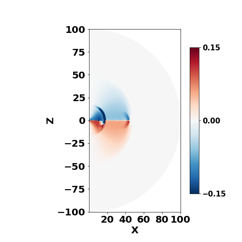
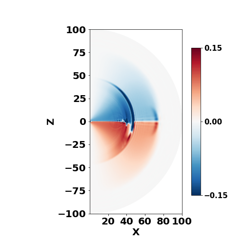
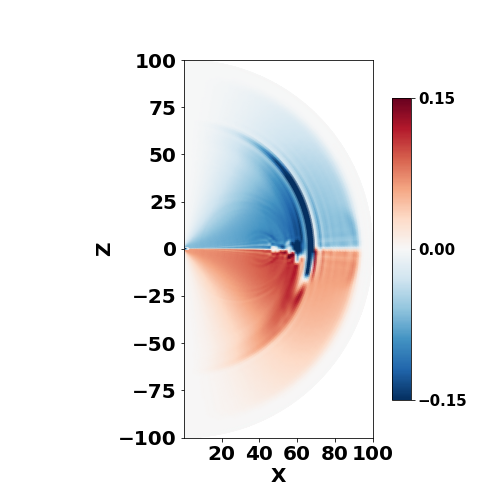
Figure 17: Same as Fig. 16, large scale view. Snapshots are taken at $t=1.6,2.5,3.2$, see Fig. 16 for zoomed-in view of the simulations. One clearly sees an electromagnetic pulse propagating through the wind.

6.3.3 Narrow anti-symmetric glitch at $\theta=\pi/2$

Here anti-symmetric shear is needed to produce a CME (otherwise the flux surfaces are just rotated as a whole, see (Lyutikov & Sharma, 2022). In order to generate anti-symmetric we chose $g(\theta)=\sin^{3}(\theta)\cos(\theta)$.

As in the previous subsection, we present our results by zooming in close to the star (Fig. 18) and showing the long time scale evolution (Fig. 19). The results are similar to what we observe for fast symmetric shearing at a band around $\pi/4$: once the shearing is introduced resulting shear Alfvén wave breaks out, reconnection is observed outside the new Y-point is formed and plasmoid instability is detected, Fig. 18d-Fig. 18e. Equilibrium state is shown in Fig. 18f.

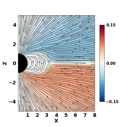
(a)

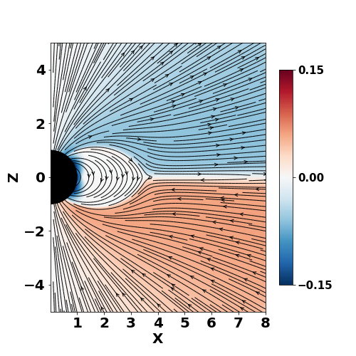
(b)

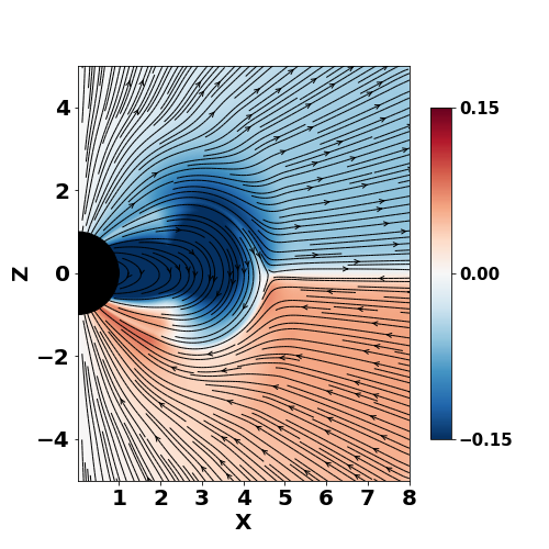
(c)

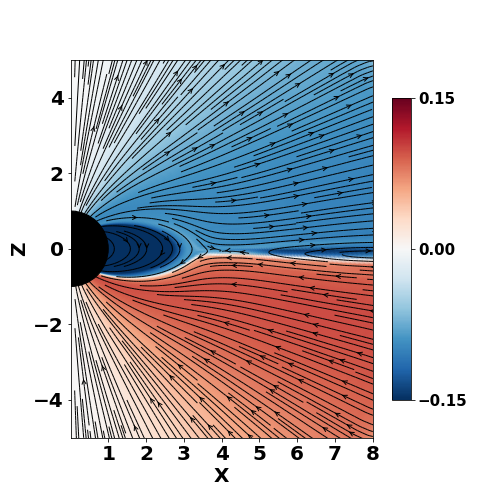
(d)

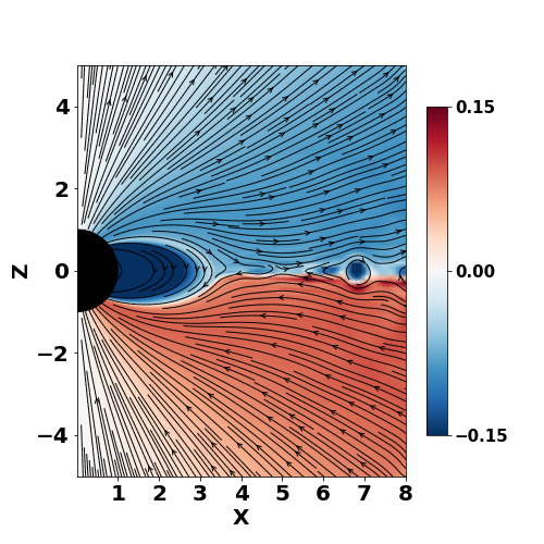
(e)

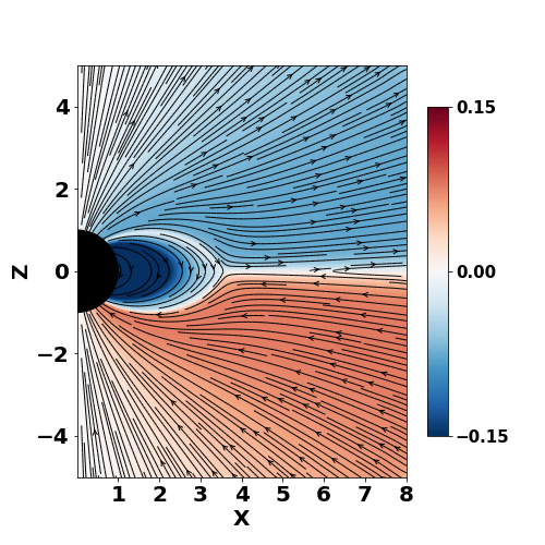
(f)

Figure 18: Anti-symmetric equatorial glitch with $g(\theta)=\sin^{3}(\theta)\cos(\theta)$, zoomed-in view. Fig. 18a is at time step just before the glitch is applied, Fig. 18b is just one time step after the initiation of the glitch. Fig. 18c shows shearing Alfvén wave breaking away from the magnetosphere. In lower row we observe formation of a new current sheet, subject to plasmoid instability. Fig. 18f is the final equilibrium state, with twisted closed field lines.

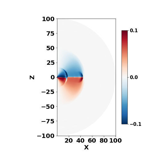
(a)

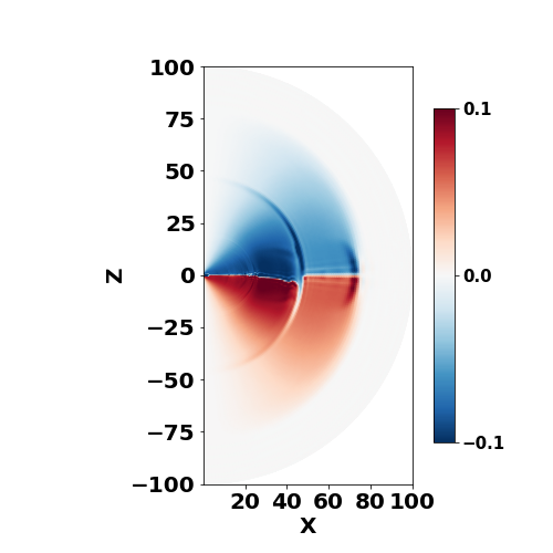
(b)

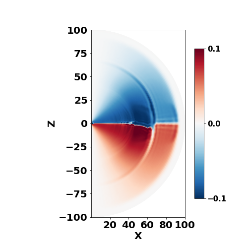
(c)

Figure 19: Anti-symmetric equatorial glitch, global view at times $t=1.6,2.5,3.2$.

6.4 Comparison of slow and fast shear, and discussion of previous results

Previously, in §5 we considered CME dynamics for slow shear. Let us compare slow and fast shear cases. Concisely: slow shear generates topologically disconnected CME that is frozen into the wind, while fast shear generates an Alfvén wave propagating through the wind. In both cases opening of the magnetosphere is followed by formation of a reconnection sheet. In the case of slow shear this opening is achieved by the inflation of the field lines followed by the break-out near the $r_{eq}$ (or near the light cylinder for weaker injections), like in the classical Solar flare models. In the case of fast shear the opening is achieved by the Alfvén packet itself, exerting a ram pressure on the closed field lines, and breaking them open.

Thus, large amplitude Alfvén waves do not break-down within the magnetosphere, as suggested by Thompson & Duncan (1995). Instead, they open-up the magnetosphere and form propagating electromagnetic pulses. The magnetosphere recovers by forming a current sheet deep inside the light cylinder, subject to plasmoid instability. Thus the Alfvén packet in the wind eventually become causally disconnected.

Our case of fast shear resembles simulations of Yuan et al. (2020) who considered the dynamics of shear Alfvén waves within the magnetosphere. In that simulation an Alfvén wave was added at the initial moment (see our §7 for similar approach) when we perform similar injection. Since the relative amplitude of the waves increases as $\delta B/B=\left(\delta B/B\right)_{\star}(r/r_{\star})^{3/2}$ for sufficiently large $\left(\delta B/B\right)_{\star}$ the waves would break with in the magnetosphere (such wave breaking is the key ingredient of Thompson & Duncan, 1995, model of magnetar flares). To avoid wave breaking Yuan et al. (2020) fine-tuned the initial amplitude of the Alfvén wave to $\left(\delta B/B\right)_{\star}$, that $\delta B/B\sim 1$ near the light cylinder.

In contrast, we generate the Alfvén wave self-consistently by shearing the foot-points. (Our simulation code use pseudo-spectral method which can’t capture breaking of the waves.) Our wave amplitude is large: the initial twist is 180 degrees. Thus, the fields in the wave quickly become much larger than the background magnetic field. The Alfvén pulse breaks out from the magnetosphere. During break-out the pre-explosion closed magnetic field lines are first stretched out, opening the magnetosphere, then reconnection “behind” the wave pulse sets in.

Our 2D fast shear simulations are generally consistent with 3D force-free simulations of Yuan et al. (2022). The similarity includes that the resulting Alfvén pulse opens the magnetosphere. The differences are as follows. First, for the non-rotating case we impose slow shear, so that the expanding structure is in an approximate force balance, while fast shear results in launching of Alfvén waves; the slow shear case also possibly leads to the detonation stage. Second, we demonstrate that the resulting Alfvén pulse within the wind leads to an EM pulse, or even anti-pulse, not a strong shock wave.

The opening of the magnetosphere in the fast shear case is somewhat different form the slow shear case. In the case of fast shear, let’s assume that the initially generated wave near the neutron star surface has amplitude $\delta B=(\Delta\phi)B_{0}$, where $(\Delta\phi)$ is a typical angle that the fields lines are sheared. The amplitude of the wave decreases as $\propto R_{NS}/r$ (both Alfvén and X-modes are excited), while the magnetospheric field decreases as $\propto(R_{NS}/r)^{3}$. The amplitude of the wave becomes lager than the guiding field for

$$\frac{r_{eq,EM}}{R_{NS}}\geq(\Delta\phi)^{-1/2}$$ (21)

This is the estimate of the opening scale of the magnetosphere for fast shear, and of the ensuing initial size of the current sheet.

Opening of the magnetosphere requires energy to be spent by the electromagnetic pulse, of the order of

$$B_{0}^{2}\left(\frac{r_{eq,EM}}{R_{NS}}\right)^{-6}r_{eq,EM}^{3}$$ (22)

Thus, more powerful pulses open the magnetosphere earlier, and experience larger energy losses.

7 Large scale dynamics of injected shear

To complement our analysis of slow and fast shear we also performed a series of experiments when a packet of shear Alfvén waves is injected into the magnetosphere (instead of the foot point motion). We inject a packet of shear Alfvén waves carrying toroidal magnetic field. In this work we focus on the scenario where the injection is performed within the magnetosphere. In what follows we conduct a thorough investigation of the system: how does the location of the ejection influences the dynamics (ejection on open versus closed field lines), and how does the flow reacts to the value of the injected flux (strong and weak ejections), and how do multiple ejections interact.

In what follows we call the injected Alfvén wave packed as flux tube, with clear understanding that the resulting structure is not topologically isolated - it is an Alfvén wave packet resembling the flux tube.

7.1 Injection procedure

The set-up in this section is as follows. We start with a dipole configuration and let the system evolve unperturbed for two time period. We then introduce a flux tube in the magnetosphere of a rotating neutron star  in approximate force equilibrium, just slightly out of force-balance. We do this by introducing external $\mathbf{B_{\phi}}$ given by Eq. (23) for a small but finite time interval $\Delta t$.

The flux tube is taken to be a torus like structure and embedded in a force-free magnetic environment with magnetic field along the azimuthal direction. The magnitude of the toroidal field inside the tube is equal to the total poloidal field of a dipole at $r=ar_{\star}$, where $a$ can be considered as the location of the center of the flux tube. The flux tube is introduced over a small radial interval at a fixed zenith angle ($\theta_{ft}$)from the z-axis.

In this subsection, since we are interested in tubes inserted inside the light cylinder we set $a=2$.

$$B_{\phi,tube}=\sqrt{B_{r}^{2}+B_{\theta}^{2}}\mbox{}$$

$$=B_{0}\sqrt{\frac{4\cos[\theta_{ft}]^{2}}{a^{6}}+\frac{\sin[\theta_{ft}]^{2}}{a^{6}}}$$ (23)

The strength and direction of the toroidal magnetic field inside the tube is controlled by the parameter $B_{0}$. For flux inserted along the magnetic wind $B_{0}$ is positive while negative when the tube is inserted against the wind. Thus, the initial configuration is just slightly unbalanced: the dipolar field at the inner edge is somewhat larger than at the outer edge of the flux tube. But as the tube is pushed radially away from the star the flux conservation quickly leads to the creation of highly over-pressurized tube. The tube then both inflates and is pushed out.

Construction of a self-confined flux tube implies that there are surface currents. Surface current $\mathbf{K}$ can be calculated via interface conditions of magnetic field (Jackson, 1999).

$$\mathbf{K}=\frac{c}{4\pi}[\mathbf{n}\times\left(\mathbf{B}_{2}-\mathbf{B}_{1}\right)]\mbox{}$$

$$\mathbf{n}\cdot\left(\mathbf{B}_{2}-\mathbf{B}_{1}\right)=0$$ (24)

Here, $B_{2}=0,B_{1}=B_{\phi,tube}$ and $\mathbf{n}$ is the unit vector from region 1 (inside the flux tube) to region 2 (outside the tube).

Since the code is sensitive to sudden changes on the magnetic field, the flux tube insertion is inserted over a finite period of time:

$$B_{\phi}=\begin{cases}B_{\phi,tube},&\text{if }t_{insertion}\leq t\leq t_{insertion}+\Delta t\\ 0,&\text{otherwise }\end{cases}$$ (25)

One important quantity is the toroidal flux added within the flux tube.

$$\Phi=\int_{S_{t}}\vec{B}\cdot\vec{n}dS$$ (26)

In the case of magnetar-generated CME, the magnetic flux carried by the flux tube originating near the surface can be estimated as

$$\Phi_{f}\sim B_{\star}R_{f}^{2}=B_{\star}\eta_{f}^{2}R_{\star}^{2}$$ (27)

where $R_{f}$ is a typical size of the active region and in the latter equality we scaled flare’s size to the radius of the neutron star, $R_{f}=\eta_{f}R_{\star}$,

The value of the added toroidal flux can be compared with the total toroidal flux within the light cylinder (in one hemisphere) generated by the rotating dipole. The model of Goldreich & Julian (1969) gives an estimate

$$\Phi_{i}\sim B_{\star}R_{\star}^{2}\left(\frac{\Omega_{\star}R_{\star}}{c}\right)$$ (28)

The injected magnetic flux therefore can be calculated via,

$$\Delta\Phi=\Phi_{f}-\Phi_{i},$$ (29)

where $\Phi_{f}$ is the toroidal flux at $t=t_{f}=t_{insertion}+\Delta t$ and $\Phi_{i}$ is the flux at $t=t_{i}=t_{insertion}$. Here $t_{insertion}$ is the simulation time step at which flux tube was introduced in the system for a duration of $\Delta t$. In this work we display our results for $t_{insertion}$ = 2 and $\Delta t=0.06$, with time expressed in term of the unperturbed rotational period of the star.

For $\Delta\Phi\sim\Phi_{f}$ we expect

$$|\frac{\Delta\Phi}{\Phi_{i}}|\sim\eta_{f}^{2}\frac{c}{\Omega_{\star}R_{\star}}\geq 1$$ (30)

Thus, the toroidal magnetic flux injected by the flare is expected to be of the order of the total toroidal magnetic flux of unperturbed magnetosphere. Our simulations’ parameters, Table 3, use similar values.

$\Delta t$	$\Phi_{i}$	$\Phi_{f}$	$\Delta\Phi$	$|\frac{\Delta\Phi}{\Phi_{i}}|$
0.03	-0.24	-0.54	-0.30	1.25
0.06	-0.24	-0.85	-0.61	2.5
0.16	-0.24	-1.43	-1.19	4.9

Table 3: Table showing toroidal flux injected to the system $\Delta\Phi$ for different values of $\Delta t$

7.2 Dynamics of shear Alfvén waves in the magnetosphere and the preceding wind

For our first sets of experiment, we add a single toroidal flux tube following the procedure described in § 7.1. The tube is launched at $a=2$ (we remind that for our basic set-up the light cylinder is at $x=5$). We explored two injection sites: at $\theta_{injection}=60^{\circ}$ (so that the injection is on closed field lines) and at $\theta_{injection}=30^{\circ}$ (so that the injection is on closed field lines). We also explored two polarizations of the injected waves which we call symmetric (so that the toroidal field in the wave is of the same sign as the toroidal field in the corresponding hemisphere of the wind), and antisymmetric (so that the toroidal field in the wave is of the same sign as the toroidal field in the corresponding hemisphere of the wind).

Though the waves are injected with similar procedures, addition of the toroidal component, this, in fact, corresponds to somewhat different modes. On the open field lines there is already $B_{\phi}$ present. This toroidal field determines the spin-down: addition of extra toroidal field modifies the spindown, see §6 and §7.3. Addition of the toroidal component on the close field lines generates both Alfvén waves (propagating mostly along the magnetic field), and compressional X-mode (propagating approximately radially).

While the Alfvén components of the resulting pulse add differently to the wind flow (depending on the strength and polarization), see Fig. 20, the X-mode component always produces a compression: a forward propagating wave, Fig. 21.

Our basic results are plotted in Fig. 20 for injection on closed field lines (”symmetric” injection). We observe that the injected flux tube first expands within the magnetosphere (top left two panels) and then propagates as an Alfvén pulse in the wind.

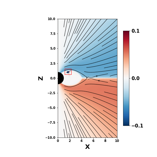
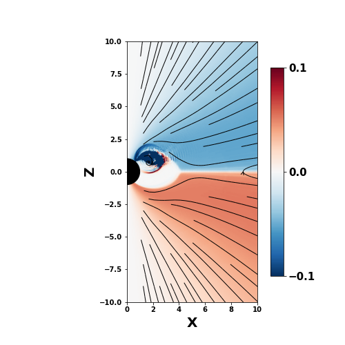
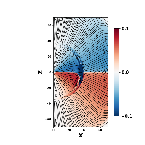
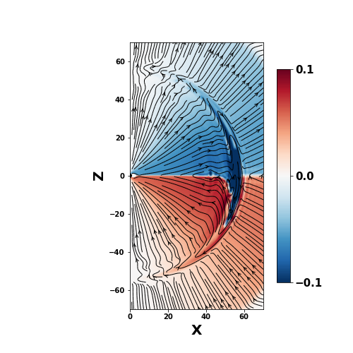
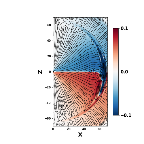
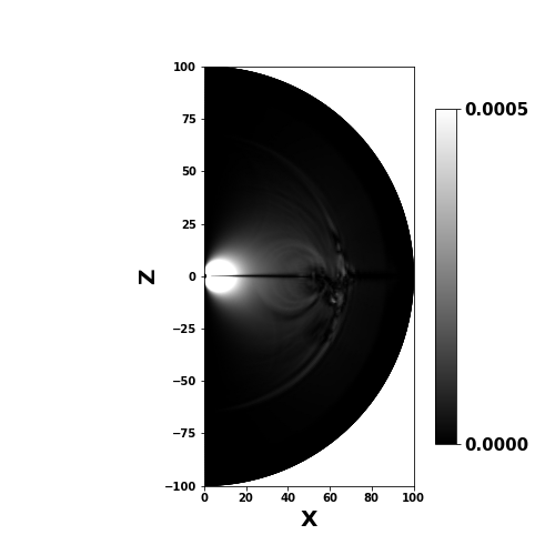
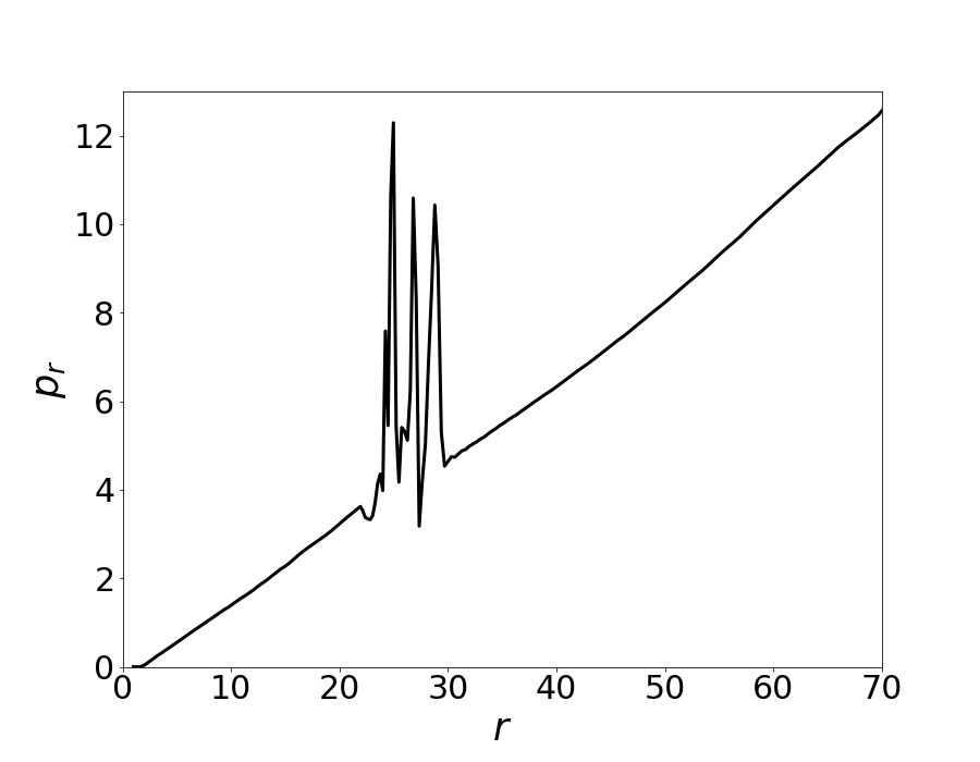
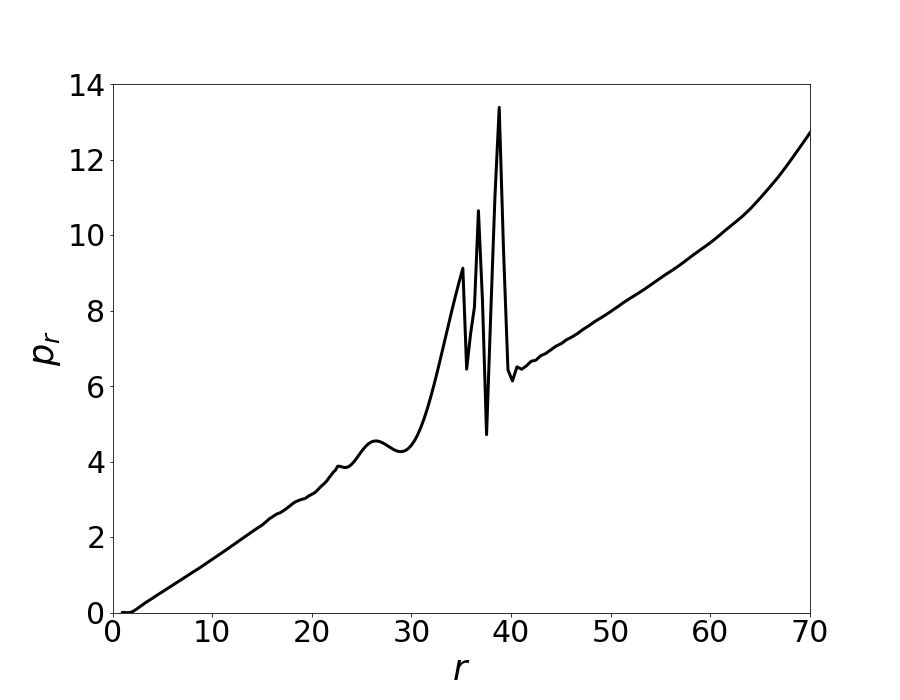
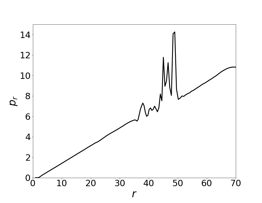
Figure 20: Flux tube/Alfvén wave packet launched on closed field lines at $60^{\circ}$ from zenith and radial distance $a=2$, ”symmetric” injection, at times $t=2.01,2.04,3.2,3.8,4.1$ (launching at $t=2$, $\Delta t=0.06$. Left and middle figures in top panel shows the zoomed-in version to capture the flux tube just after the launch. In the first plot the injected flux tube is a small patch, highlighted within a rectangle for visual clarity. We observe that the flux tube expands quickly within the light cylinder. The right grayscale figure in the middle panel shows the absolute value of effective magnetic field $(B^{2}-E^{2})\times r^{2}\sin^{2}\theta$ at $t=4.1$; it demonstrates that with the the flux tube Alfvén pulse there are no large variations of the effective magnetic field. Bottom panel shows the magnitude of radial momentum $p_{r}$ as a function of radial distance r for a slice at $60^{\circ}$ from the pole at $t=\{2.9,3.2,3.5\}$. A forward-propagating pulse is clearly seen. We also repeated the calculations for angular slice at $120^{\circ}$ and the results were similar.

To further elucidate the underlying dynamics in Fig. 21 we compare later behavior for “antisymmetric” injection at two locations: $\theta=30^{\circ}$ (left panels) and $\theta=60^{\circ}$ (right panel). In both cases the injection is “weak” - meaning that the injected toroidal flux is somewhat smaller than (28). The two cases are clearly different: for “antisymmetric” injection on open field lines a backward propagating wave is launched (in the panel 21.a the radial momentum within the wave is smaller than that of the wind.

At the same time the similar injection but on closed field lines (right panels in Fig. 21) creates forward propagating pulse. The reason for the differences is the following. For “antisymmetric” injection on open field lines the resulting Alfvén pulse resembles the magnetospheric glitch, §6 - regions with smaller toroidal field propagate slower. (We also verified that in case of “strong antisymmetric” injection, when the injected toroidal flux is larger than (28), the resulting pulse is forward-propagating.

Qualitatively, using Michel’s solution (17) a local toroidal magnetic field corresponds to some local effective angular velocity. Reducing local toroidal magnetic field (for weak antisymmetric injection) reduces the effective angular velocity and the radial momentum. Since the radial momentum $p_{r}$ is a quadratic function of the field, strong antisymmetric injection (so that the total toroidal field is larger inside the pulse than in the surrounding wind) produces forward propagating pulse.

Injection on the closed field lines proceeds differently. For “mild” injection, the added toroidal field on the closed field lines corresponds to fast mode regardless of the polarization. The fast mode first propagates through the magnetosphere and then creates compression of the field in the wind. The resulting pulse is always forward propagating.

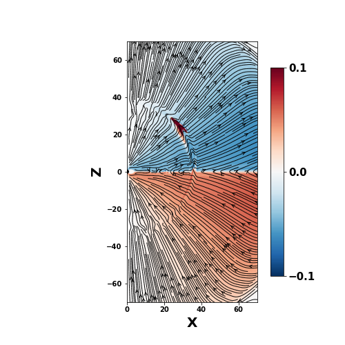
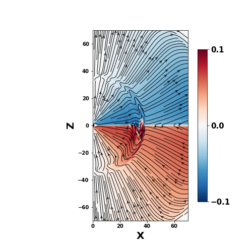
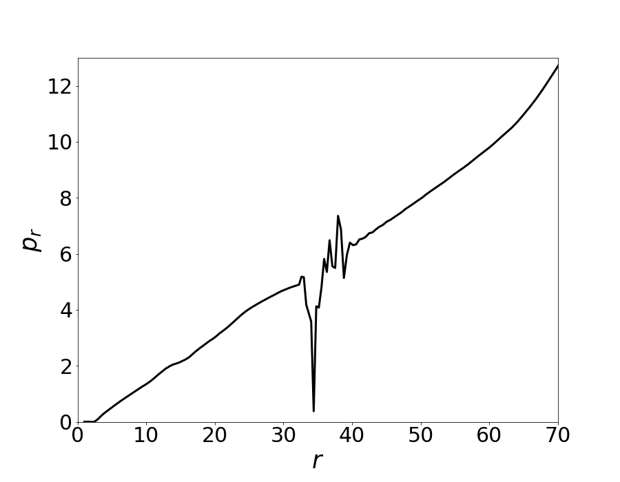
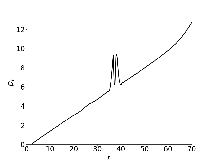
Figure 21: Comparison of injections on open field lines $\theta=30^{\circ}$ (left column) and closed field $\theta=60^{\circ}$ (right column). Weak “antisymmetric” injection. Notice that injection on open field lines produces a pulse that is backward propagating through the wind. For injection on closed field lines, the fast mode propagating with the magnetosphere creates an electromagnetic pulse that propagates in a forward direction through the wind independently on the initial polarization of the pulse.

7.3 Multiple injection events

We end this section by considering the scenario of multiple flux tubes. Here we add two flux tubes, the first one at $t=t_{insertion}$, and second one at $t=1.5t_{insertion}$ with time expressed in terms of the rotational period of the star. The first tube is weaker and launched agains the wind (anti-symmetric scenario) while the second tube is stronger and launched along the wind. We consider injections on open field lines $\theta=30^{\circ}$ and closed field $\theta=60^{\circ}$. We show a snapshot of such multi flux tube system in Fig. 22a ,Fig. 22b The two tubes don’t catch up, even if the second one is more powerful and the first is “weak-antisymmetric” launched on open field lines (hence propagating backwards through the wind).

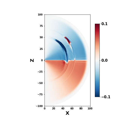
(a)

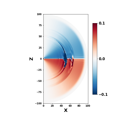
(b)

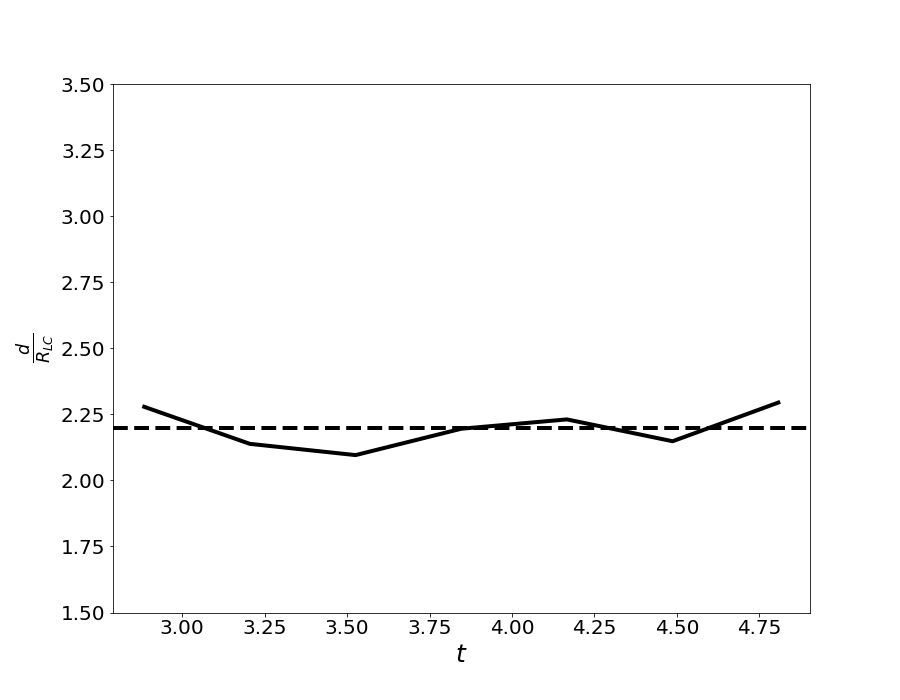
(c)

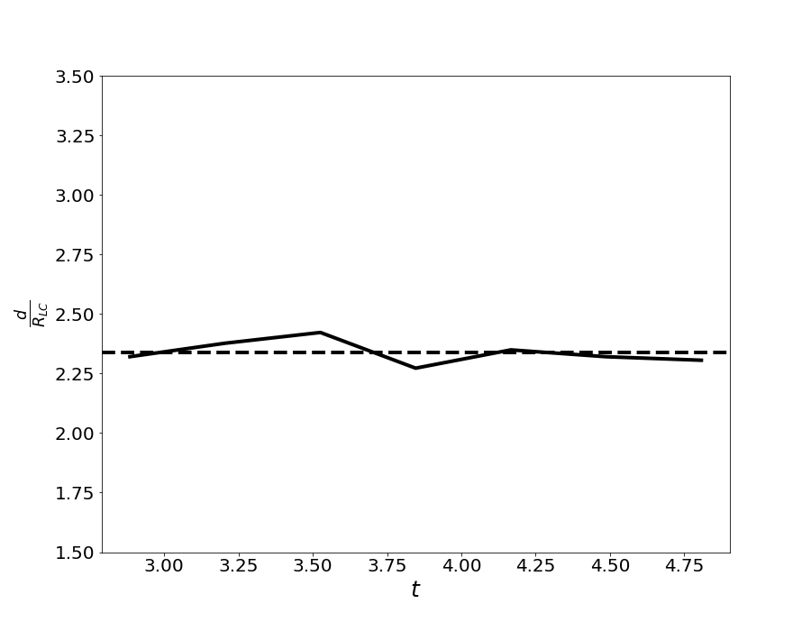
(d)

Figure 22: Multiple injection events. Two tubes are injected inside the light cylinder  at spherical radius $a=2$. Injection occurs at $30^{\circ}$ (left column, on open field lines) and $60^{\circ}$ (right column, on open field lines). The first tube is weak-antisymmetric, the second tube was launched half rotational period after the first one. Bottom row: time evolution of the distance between the two flux tubes. Solid line represents the separation between the tubes as a function of time whereas the dashed line shows the average separation. As observed, the separation between the injections remains (approximately) the same.

This is clearly a result of relativistic kinematics, modified by the fact that the bulk flow is accelerating. In fact, Alfvén waves propagating in the Michel’s wind can be considered non-perturbatively, Lyutikov (2011) and §6. Such waves can be parametrized by the local spin $\Omega_{1,2}\neq\Omega_{0}$ ($\Omega_{0}$ is constant spin of the star). One then finds the location of the first wave at time $t$ after leaving the light cylinder:

$$R_{1}=\frac{1}{2}\left(t+\frac{1}{\Omega_{0}}-\frac{\Omega_{0}}{\Omega_{1}^{2}}\right)+\sqrt{1+\frac{\left(\Omega_{1}^{2}(1+t\Omega_{0})-\Omega_{0}^{2}\right){}^{2}}{4\Omega_{0}^{2}\Omega_{1}^{2}}}\frac{1}{\Omega_{1}}\approx t+\frac{1}{\Omega_{0}}-\frac{\Omega_{0}}{\Omega_{1}^{2}}+\frac{1}{t\Omega_{1}^{2}}$$ (31)

where $R_{(}0)=1/\Omega_{0}$ (wave is launched at time $t=0$ at the light cylinder); the latter relation is for $t\gg 1/\Omega_{0}$. Eq. (31) gives the location of the Alfvén pulse propagating through accelerating wind.

If a second Alfvén pulse is launched after time $\Delta t$ with $\Omega_{2}\geq\Omega_{1}$, the collision will occur approximately at

$$t_{coll}\Omega_{0}\approx\left(1+\frac{{\Delta t}\Omega_{1}^{2}\Omega_{2}^{2}}{\Omega_{0}\left(\Omega_{1}^{2}-\Omega_{2}^{2}\right)}\right)^{-1}\approx\frac{1}{2}\Omega_{0}^{2}\left(\frac{1}{\Omega_{1}^{2}}-\frac{1}{\Omega_{2}^{2}}\right)$$ (32)

where the last relation assumes that the two pulses are separated by one rotation. Typical collision times are long and not captured by our simulations. When the waves eventually catch up at $r\gg R_{LC}$, the interaction will be resemble interaction between two non-linear packets of fast modes.

8 Conclusion: whence to FRB

In this work we continue, following Lyutikov (2022); Barkov et al. (2022), exploration of the dynamics of the relativistic magnetized explosions: how relativistic magnetically-driven explosions are produces by magnetar, and how they propagate through the preexisting magnetized wind. To search for answers we performed multiple 2D numerical simulations of a neutron star magnetosphere and the winds. The simulations focused on several different but related phenomenons: production of magnetic flares via shearing of the foot-points of the magnetic field lines, and evolution of relativistic flux tube(s)/Alfvén pulses in magnetars’ winds.

Two regimes of foot-points shearing we considered: (i) slow shear, so that the whole inflated magnetic arc structure is in a state of causal contact; (ii) fast shear, so that the corresponding dynamics resembles large amplitude Alfvén waves injected into the magnetosphere.

We stress again the importance of magnetic loading of magnetar flares (Lyutikov, 2022; Barkov et al., 2022): an injected flux tube/plasmoid looses a lot of energy trying to break out from the magnetosphere. For example, we expect that a fraction of the injected magnetic energy $E_{CME,0}$ will be emitted in X-rays. Yet the energy that gets deposited into the wind even in the super-critical case is always much smaller at least by the small numerical factor $\eta_{E}$ (the ratio of injected energy to the total magnetospheric energy); for the flux tube scenario the decrease is even more dramatic, $\propto\eta_{E}^{2}$, see Table 1. For milder flares the wind adjusts to the perturbation right near the light cylinder, so no energy in deposited in the wind.

For subcritical injections, which do not experience detonation inside the light cylinder, the resulting CME is completely “cold turkey”: a structure in force balance and advected passively with the wind. If the CME’s energy exceeds the critical and detonation occurs, then still only small fraction of the initial energy, at most $\sim\eta_{E}$, is transferred to the wind in the form of EM pulse.

We conclude that:

• For slow shear, the Solar flare paradigm:

  • there are two possible stages of CME expansion within the magnetosphere: for sufficiently large injection, a CME experiences internal detonation at some radius $r_{eq}$, when it starts expanding relativistically within the magnetosphere and loses causal connection.

  • the magnetospheric dynamics depends both on the large scale structure and on the location of shearing foot points: to generate rare powerful events shear must occur on field lines that “close in” near the star; otherwise numerous weak events are generated.

  • Ejected magnetic blobs, CMEs, are frozen into the wind

• For fast shear, the Star quake paradigm:

  • Shearing of foot-points leads to the generation of Alfvén wave; the pressure of the Alfvén leads to opening of the magnetosphere (no wave breaking).

  • Resulting perturbations propagate in the wind as shear Alfvén waves, with no breaking

  • multiple shear Alfvén waves are unlikely to collide within relativistically accelerating wind.

• In both cases of slow and fast shear no considerable dissipation occurs in the wind zone. In both cases after the ejection the magnetosphere first opens; afterwards the newly closed magnetosphere is smaller, and recovers resistively.

Our results are complementary to those of Barkov et al. (2022), who investigated the dynamics of magnetic explosions with complicated, linked magnetic internal stricture. Barkov et al. (2022) showed, using both relativistic MHD and force-free approaches, that there is a clear regime of magnetic explosions - detonation. In this regime in MHD the expansion of a spheromak becomes supersonic, in the force-free case we see spheromak torn apart, and also becoming causally disconnected.

Our results make a consistent picture: powerful strongly magnetized ejected blobs/flux tube makes minimal distortion in the wind. They either quickly reach force-balance with the wind, and propagate self-similarly, without producing shocks and/or dissipative structures, or propagate as highly weakened electromagnetic disturbances. This picture is in sharp contrast with the hydrodynamics, where over-pressurized regions create strong dissipative shock.

Our results have implications for the generation of FRBs.

• FRBs as Coronal Mass Ejections - large and small. FRBs show large range of luminosities (CHIME/FRB Collaboration et al., 2020; Shin et al., 2022), which raises an obvious question: what’s the control parameter that defines (both X-ray and radio) luminosity of magnetars’ bursts/flares? The overall size involved in a flare is one obvious parameters. Another is the strength of the magnetic field - both determine total energetics.

  In the Solar flare paradigm of magnetar flares, the magnetic field also enters via the rate of shearing the foot-point: the shearing rate is $\propto$ magnetic field (Goldreich & Reisenegger, 1992); thus, qualitatively, the magnetar activity is a $B^{3}$ function of the magnetic field (Lyutikov, 2015).

  In the present work we find that other, less clearly measured properties play a role: (i) evolution of a CME within magnetosphere proceeds in different regimes depending on the injected energy (possibly a detonation); (ii) location of the shear; (iii) overall structure of the magnetosphere. If shearing is done near the fields that extend far out from the star, then the twist is easily released in many small flares. (Along a given field line the twist concentrates near the regions of weakest magnetic field, hence at the highest point in the magnetosphere.) In order to produce rare and powerful explosions the shearing should be done at the foot-points of field lines that close in, roughly speaking, within a stellar radius.

  Qualitatively, a twist of a given magnetic field line concentrates near the points where the guiding field is the weakest - at the furthest extent. It is there that the stability is determined. For field lines extending to large distances, the guiding field is small, so that the kink instability is easily initiated at small twists. The system then gets rid of the twist in many small events.

  Finally, the presence of the light cylinder effectively impedes the storage of the magnetic energy. If an inflated flux tube reaches the light cylinder, it opens up and releases the twist this limits the amount of magnetic energy that can be stored. Thus, to produce strong flares the spin period should not be too short.

• Dynamics of CMEs/electromagnetic pulses in the preceding wind. Our results on the wind dynamics are in some contradiction to the “wind models” of FRBs (e.g.  Lyubarsky, 2014; Beloborodov, 2017; Metzger et al., 2019; Thompson, 2022). For slow shear, the Solar flare paradigm, energetically mild CME (non-detonating) produce minimal distortion of the wind: topologically disconnected structures (“magnetic shells”) come into force balance close to the light cylinder, and are then passively advected with the flow. In the super-critical detonating case, a highly weakened electromagnetic pulse is launched into the wind. For fast shear, the Starquake paradigm, the energy is quickly deposited into the magnetosphere in a form of Alfvén and X-modes that may also open the magnetosphere. In doing so, the wave energy is deposited into the magnetosphere, so is lost by the pulse. More powerful pulses open the magnetosphere earlier and suffer larger energy losses.

  In passing we note that the original shock model of Gallant et al. (1992); Hoshino et al. (1992), envisioned to explain months-long variability of Crab Nebula wisps, involves interaction of the relativistic wind with a heavy ejecta. In that case the cyclotron instability occurs in the termination shock of the wind, with only mildly relativistic post-shock flow. It is not applicable to generation of millisecond (and even shorter) radio pulses in FRBs.

9 Acknowledgements

This work had been supported by NASA grants 80NSSC17K0757 and 80NSSC20K0910, NSF grants 1903332 and 1908590. We would like to thank Spiro Antiochos, Jens Mahlmann, Bart Ripperda and Chris Thomson for comments and discussions. The work of the organizers of the “Plenty of Room at the Bottom: Fast Radio Bursts in our Backyard” workshop is acknowledged.

10 Data availability

The data underlying this article will be shared on reasonable request to the corresponding author.

Appendix A Numerical Method

In this paper, we study the dynamics of sheared magnetospheres using time-dependent numerical simulations with the code PHAEDRA (Parfrey et al., 2012). The code solves Maxwell’s equations together with ideal constraints

$$\mathbf{J}.\mathbf{E}=0\mbox{}$$

$$\mathbf{B^{2}}-\mathbf{E^{2}}\geq 0$$ (33)

in spherical, axisymmetric geometry.

The simulation domain extends from $r_{in}=r_{\star}$, the neutron star radius to the outer boundary $r_{out}$. For plasmoid ejection simulations, we set up the outer boundary at $r=10r_{\star}$ whereas for flux tube simulations the the outer boundary was set at $r=100r_{\star}$. We use smooth coordinate mapping for the radial grid, while the grid is equi-spaced in $\theta$ direction. The computational mesh consists of $280\times 180$ cells in $(r,\theta)$ directions respectively.

Our simulation region has two major boundaries: the inner boundary i.e. the surface of the star and the outer boundary defined by size of our simulation box. We assume axisymmetry as well as symmetry about the equatorial plane. The normal component of the magnetic field, $B_{r}$, and the tangential components of the electric field are continuous across the surface, and therefore are known. The required boundary conditions at $r=r_{\star}$ are

$$B_{r}=B_{r}(\theta)\mbox{}$$

$$E_{\theta}=-\Omega B_{r}\sin\theta\mbox{}$$

$$E_{\phi}=0$$ (34)

For plasmoid ejection simulation, we introduce shearing after one rotation period by simply modifying the net angular velocity at the surface by $\Omega=\Omega+\omega_{s}$. For rotating cases, the rotational angular velocity of the star $\Omega$ is set as $0.2$ throughout the entire work.

Appendix B Dipole-plus-quadrupole configurations

In this case fairly simple analytical results can guide us for the choice of shearing location. The flux function for dipole and quadrupole, normalized to magnetic field at the pole are

$$P_{d}=\frac{\sin^{2}\theta}{r}\frac{B_{p}R^{3}}{2}\mbox{}$$

$$P_{q}=\frac{\sin(2\theta)\sin\theta}{r^{2}}\frac{B_{q}R^{4}}{4}\mbox{}$$

$${\bf B}_{d,q}=\nabla P_{d,q}\times\nabla\phi$$ (35)

Total field is a linear sum

$$P_{tot}=P_{d}+\mu_{q}P_{q}$$ (36)

where $\mu_{q}$ parametrizes the relative strength of the dipole and quadrupole. We use $\mu_{q}=2$: this makes the magnetic field at one pole 3 times larger than pure dipole, while at the other pole magnetic field equal in value to the dipole value, but with the reverse sign.

We find special points:

• Zero point at anti-pole corresponds to $\mu_{q}=1$

• edge of the southern dome $\cos\theta_{dome}=-1/\eta$ ($\theta_{dome}=2\pi/3$ for $\mu_{q}=2$).

• Upper polar cap. Furthest point at $R_{LC}=r\sin\theta_{Y}$, ($\theta_{Y}$ is the angle of the Y-point

  $$\eta=-\frac{6\cot(\theta_{Y})}{5\cos(2\theta_{Y})+3}\frac{R_{LC}}{R}$$ (37)

  For $R_{LC}/R=5$ and $\eta=2$, $\theta_{Y}=1.4480$ ($\theta_{Y}$ cannot be smaller than $\cos(2\theta_{Y})=-3/5$). Y-point is at $r=R_{LC}/\sin\theta_{Y}\to 5.037$.

• At the last open field line

  $$P_{tot}^{(0)}=\frac{\sin^{3}\left(\theta_{Y}\right)\cos\left(2\theta_{Y}\right)}{5\cos\left(2\theta_{Y}\right)+3}\frac{1}{R_{LC}}$$ (38)

  Last closed field lines is given by

  $$r^{(0)}=\frac{\sin^{2}(\theta)\pm\sin(\theta)\sqrt{\sin^{2}(\theta)+8\eta P_{tot}^{(0)}\cos(\theta)}}{4P_{tot}^{(0)}}$$ (39)

  Maximal extent is when they are equal,

  $$\cos\theta_{max}=4P_{tot}^{(0)}\mu_{q}-\sqrt{1+(4P_{tot}^{(0)}\eta)^{2}}$$ (40)

  Polar cap polar angles are

  $$\theta_{PC,1}=0.267\mbox{}$$

  $$\theta_{PC,2}=1.96$$ (41)

Appendix C Rotating stars with no foot-point shearing

As a preliminary investigation, we considered rotating but unsheared configurations. Rotation adds a characteristic scale to the problem viz., the radius of the light cylinder $R_{LC}$. The field lines opens to infinity beyond the light cylinder. We start with a non-rotating neutron star and bring it to final rotational velocity $\Omega_{\star}$ and then allowed to relax to a steady equilibrium state.

We first consider the case of an aligned neutron star in purely dipolar field, and with no shearing of the magnetic field lines. We expect the solution to resemble that given by (Michel, 1973) (Eq. (17)), once the equilibrium has been achieved. We compared the radial momentum from simulations for a fixed $\theta$ with those generated from simulations and the values were in excellent agreement (Fig. 24). We also observe few weak plasmoid ejection events, consistent with Parfrey et al. (2013), Fig. 25.

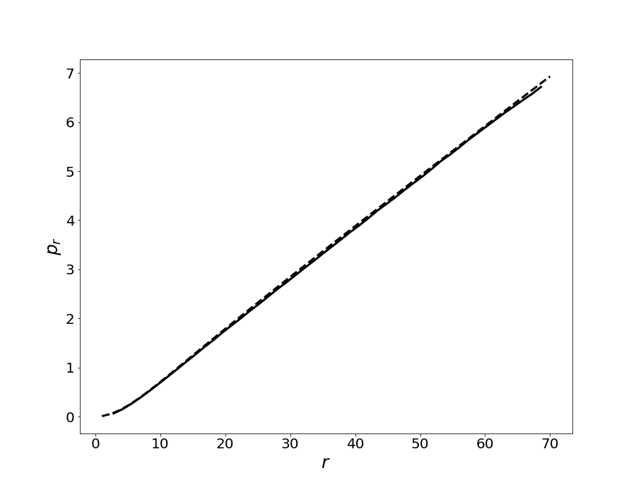
Figure 24: Radial momentum (solid) from analytical expression (Eq. (17)) and (dashed) for a simple dipole with no flux tube from numerical simulation data at $\theta=30^{\circ}$

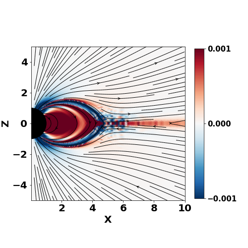
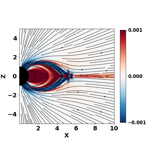
Figure 25: Toroidal current $(J_{\phi})$ for an aligned rotating dipole ($\Omega=0.2$) with no shearing at two consecutive time slice clearly showing plasmoid ejection.

References

- Aly (1980) Aly J. J., 1980, A&A, 86, 192
- Aly (1991) Aly J. J., 1991, apjl, 375, L61
- Antiochos et al. (1999) Antiochos S. K., DeVore C. R., Klimchuk J. A., 1999, apj, 510, 485
- Antiochos et al. (2007) Antiochos S. K., DeVore C. R., Karpen J. T., Mikić Z., 2007, apj, 671, 936
- Barkov & Popov (2022) Barkov M. V., Popov S. B., 2022, MNRAS, 515, 4217
- Barkov et al. (2022) Barkov M. V., Sharma P., Gourgouliatos K. N., Lyutikov M., 2022, ApJ, 934, 140
- Beloborodov (2017) Beloborodov A. M., 2017, apjl, 843, L26
- Bochenek et al. (2020) Bochenek C. D., Ravi V., Belov K. V., Hallinan G., Kocz J., Kulkarni S. R., McKenna D. L., 2020, nat, 587, 59
- Bogovalov (1999) Bogovalov S. V., 1999, aap, 349, 1017
- CHIME/FRB Collaboration et al. (2020) CHIME/FRB Collaboration et al., 2020, nat, 587, 54
- CHIME/FRB Collaboration et al. (2022) CHIME/FRB Collaboration et al., 2022, nat, 607, 256
- Contopoulos et al. (1999) Contopoulos I., Kazanas D., Fendt C., 1999, apj, 511, 351
- Cordes & Chatterjee (2019) Cordes J. M., Chatterjee S., 2019, araa, 57, 417
- Forbes (2000) Forbes T. G., 2000, J. Geophys. Res., 105, 23153
- Gallant et al. (1992) Gallant Y. A., Hoshino M., Langdon A. B., Arons J., Max C. E., 1992, ApJ, 391, 73
- Goldreich & Julian (1969) Goldreich P., Julian W. H., 1969, apj, 157, 869
- Goldreich & Reisenegger (1992) Goldreich P., Reisenegger A., 1992, ApJ, 395, 250
- Gourgouliatos et al. (2013) Gourgouliatos K. N., Cumming A., Reisenegger A., Armaza C., Lyutikov M., Valdivia J. A., 2013, mnras, 434, 2480
- Gralla & Jacobson (2014) Gralla S. E., Jacobson T., 2014, MNRAS, 445, 2500
- Hoshino et al. (1992) Hoshino M., Arons J., Gallant Y. A., Langdon A. B., 1992, ApJ, 390, 454
- Hurley et al. (2005) Hurley K., et al., 2005, nat, 434, 1098
- Jackson (1999) Jackson J. D., 1999, Classical electrodynamics; 3rd ed.. Wiley, New York, NY
- Kaspi & Beloborodov (2017) Kaspi V. M., Beloborodov A. M., 2017, araa, 55, 261
- Khangulyan et al. (2022) Khangulyan D., Barkov M. V., Popov S. B., 2022, ApJ, 927, 2
- Komissarov (2006) Komissarov S. S., 2006, MNRAS, 367, 19
- Komissarov & Barkov (2007) Komissarov S. S., Barkov M. V., 2007, MNRAS, 382, 1029
- Komissarov et al. (2007) Komissarov S. S., Barkov M., Lyutikov M., 2007, mnras, 374, 415
- Levin & Lyutikov (2012) Levin Y., Lyutikov M., 2012, mnras, 427, 1574
- Li & Luhmann (2005) Li Y., Luhmann J. G., 2005, in AGU Spring Meeting Abstracts. pp SH51C–08
- Lyubarsky (2014) Lyubarsky Y., 2014, mnras, 442, L9
- Lyutikov (2003) Lyutikov M., 2003, MNRAS, 346, 540
- Lyutikov (2006) Lyutikov M., 2006, mnras, 367, 1594
- Lyutikov (2010) Lyutikov M., 2010, Phys. Rev. E, 82, 056305
- Lyutikov (2011) Lyutikov M., 2011, Phys. Rev. D, 83, 124035
- Lyutikov (2013) Lyutikov M., 2013, arXiv e-prints, p. arXiv:1306.2264
- Lyutikov (2015) Lyutikov M., 2015, mnras, 447, 1407
- Lyutikov (2021) Lyutikov M., 2021, ApJ, 922, 166
- Lyutikov (2022) Lyutikov M., 2022, mnras, 509, 2689
- Lyutikov (2023) Lyutikov M., 2023, MNRAS,
- Lyutikov & Hadden (2012) Lyutikov M., Hadden S., 2012, Phys. Rev. E, 85, 026401
- Lyutikov & Popov (2020) Lyutikov M., Popov S., 2020, arXiv e-prints, p. arXiv:2005.05093
- Lyutikov & Sharma (2022) Lyutikov M., Sharma P., 2022, MNRAS, 513, 1947
- Lyutikov et al. (2016) Lyutikov M., Burzawa L., Popov S. B., 2016, mnras, 462, 941
- Mereghetti (2008) Mereghetti S., 2008, aapr, 15, 225
- Mereghetti et al. (2020) Mereghetti S., et al., 2020, apjl, 898, L29
- Metzger et al. (2019) Metzger B. D., Margalit B., Sironi L., 2019, MNRAS, 485, 4091
- Michel (1973) Michel F. C., 1973, apjl, 180, L133
- Mikic & Linker (1994) Mikic Z., Linker J. A., 1994, ApJ, 430, 898
- Palmer et al. (2005) Palmer D. M., et al., 2005, nat, 434, 1107
- Parfrey et al. (2012) Parfrey K., Beloborodov A. M., Hui L., 2012, mnras, 423, 1416
- Parfrey et al. (2013) Parfrey K., Beloborodov A. M., Hui L., 2013, ApJ, 774, 92
- Petroff et al. (2019) Petroff E., Hessels J. W. T., Lorimer D. R., 2019, aapr, 27, 4
- Popov & Postnov (2013) Popov S. B., Postnov K. A., 2013, arXiv e-prints, p. arXiv:1307.4924
- Ridnaia et al. (2021) Ridnaia A., et al., 2021, Nature Astronomy, 5, 372
- Ripperda et al. (2019) Ripperda B., Porth O., Sironi L., Keppens R., 2019, mnras, 485, 299
- Shin et al. (2022) Shin K., et al., 2022, arXiv e-prints, p. arXiv:2207.14316
- Thompson (2022) Thompson C., 2022, arXiv e-prints, p. arXiv:2209.11136
- Thompson & Duncan (1995) Thompson C., Duncan R. C., 1995, MNRAS, 275, 255
- Thompson & Duncan (2001) Thompson C., Duncan R. C., 2001, ApJ, 561, 980
- Usov (1992) Usov V. V., 1992, Nature, 357, 472
- Vourlidas et al. (2002) Vourlidas A., Buzasi D., Howard R., Esfandiari E., 2002, J. Kuijpers (Noordwijk: ESA), 91
- Wolfson & Low (1992) Wolfson R., Low B. C., 1992, ApJ, 391, 353
- Wood et al. (2014) Wood T. S., Hollerbach R., Lyutikov M., 2014, Physics of Plasmas, 21, 052110
- Younes et al. (2022) Younes G., et al., 2022, arXiv e-prints, p. arXiv:2210.11518
- Yuan et al. (2020) Yuan Y., Beloborodov A. M., Chen A. Y., Levin Y., 2020, apjl, 900, L21
- Yuan et al. (2022) Yuan Y., Beloborodov A. M., Chen A. Y., Levin Y., Most E. R., Philippov A. A., 2022, ApJ, 933, 174