Coherent emission in pulsars, magnetars and Fast Radio Bursts: reconnection-driven free electron laser

Abstract

We develop a model of the generation of coherent radio emission in the Crab pulsar, magnetars and Fast Radio Bursts (FRBs). Emission is produced by a reconnection-generated beam of particles via a variant of Free Electron Laser (FEL) mechanism, operating in a weakly-turbulent, guide-field dominated plasma. We first consider nonlinear Thomson scattering in a guide-field dominated regime, and apply to model to explain emission bands observed in Crab pulsar and in Fast Radio Bursts. We consider particle motion in a combined fields of the electromagnetic wave and the electromagnetic  (Alfvenic) wiggler. Charge bunches, created via a ponderomotive force, Compton/Raman scatter the wiggler field coherently. The model is both robust to the underlying plasma parameters and succeeds in reproducing a number of subtle observed features: (i) emission frequencies depend mostly on the length $\lambda_{t}$ of turbulence and the Lorentz factor of the reconnection generated beam, $\omega\sim\gamma_{b}^{2}(c/\lambda_{t})$ - it is independent of the absolute value of the underlying magnetic field. (ii) The model explains both broadband emission and the presence of emission stripes, including multiple stripes observed in the High Frequency Interpulse of the Crab pulsar. (iii) The model reproduces correlated polarization properties: presence of narrow emission bands in the spectrum favors linear polarization, while broadband emission can have arbitrary polarization. (iv) The mechanism is robust to the momentum spread of the particle in the beam. We also discuss a model of wigglers as non-linear force-free Alfven solitons (light darts).

1 Introduction: challenges of coherent emission in Crab, magnetars and Fast Radio Bursts

Pulsar emission mechanisms remain illusive for more than half a century (Goldreich & Keeley, 1971; Ruderman & Sutherland, 1975; Cheng & Ruderman, 1977; Beskin et al., 1988; Melrose, 1992; Melrose & Gedalin, 1999; Melrose, 2000; Lyutikov et al., 1999; Melrose, 2017; Beskin, 2018). Until recently, the rotationally-driven paradigm was prevailing: rotating magnetic fields generate parallel electric fields, that accelerate particles with unstable distribution function; this eventually lead to production of coherent emission (Ruderman & Sutherland, 1975; Fawley et al., 1977; Arons & Scharlemann, 1979; Hibschman & Arons, 2001)

During the last years a new consensus about generation of pulsar radio emission emerged, especially in application to Crab Main Pulse and Interpulse (MP and IP): radio emission is reconnection-driven, not rotationally-driven (there are likely several types of emission mechanism operating in pulsars). Reconnection has been suggested as a source of coherent emission in radio pulsars (Istomin, 2004), magnetar (Lyutikov, 2002, 2006). and FRBs (Popov & Postnov, 2013; Lyubarsky, 2020; Lyutikov, 2017; Lyutikov & Popov, 2020). The reconnection-driven generation of radio pulses is becoming a dominant theoretical concept for generation of Crab MP and IP (Bai & Spitkovsky, 2010; Arons, 2012; Chen & Beloborodov, 2014; Cerutti et al., 2015a, 2016; Cerutti & Beloborodov, 2017; Wang et al., 2019; Lyubarsky, 2019; Contopoulos & Stefanou, 2019; Philippov et al., 2019). It is not clear why/how Crab is different from most other pulsars, in that its radio emission is dominated by the reconnection-driven, not rotationally-driven processes.

One of the most interesting property of Crab radio emission is observations of numerous emission stripes in Crab High Frequency interpulse (Moffett & Hankins, 1999; Hankins & Eilek, 2007a; Hankins et al., 2016; Eilek & Hankins, 2016).

s

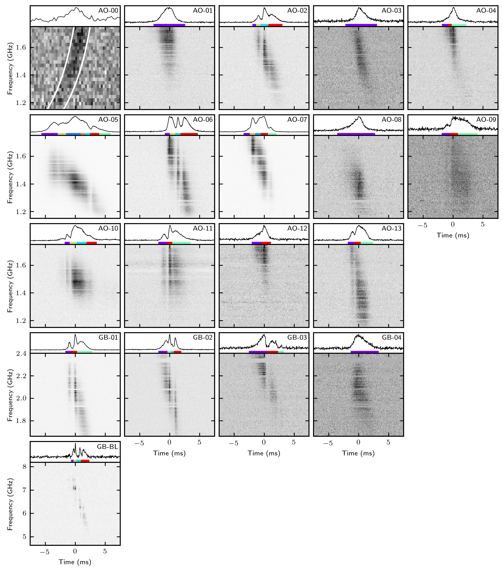
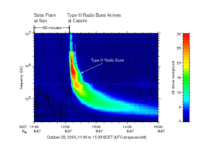
Figure 1: Left panel: Example of narrow-band emission stripes in Crab High Frequency Interpulse Eilek & Hankins (2016). There is at least more than a dozen bands extending from few to tens of GHz. Middle panel: narrow drifting emission bands seen in FRB 121102 Hessels et al. (2019). Right panel: Solar type-III radio burst showing similar downward frequency drifts to FRBs.

Emission is composed of at least a dozen relatively narrow emission bands, almost equally spaced in frequency (spacing increases with frequency at a rate of $6\%$). We consider these stripes being the properties of the emission mechanism, not propagation (Lyutikov, 2007). It is one of the most intricate properties of pulsar radio emission - explaining it will be a strong argument in favor of any model of pulsar radio emission.

Discoveries related to Fast Radio Bursts (Petroff et al., 2019; Cordes & Chatterjee, 2019) renewed interest in production of coherent emission in compact objects. Simultaneous observations of radio and X-ray bursts (CHIME/FRB Collaboration et al., 2020; Ridnaia et al., 2020; Bochenek et al., 2020; Mereghetti et al., 2020) establishes magnetospheric origin of FRBs loci (Lyutikov & Popov, 2020). Observations of downward frequency drifts (Hessels et al., 2019; The CHIME/FRB Collaboration et al., 2019a, b; Josephy et al., 2019) are consistent with the original prediction for magnetospheric origin of magnetar radio flares (Lyutikov, 2002). Recent observations of PA swings (Nimmo et al., 2020), originally predicted by Lyutikov (2020c), further confirm magnetospheric origin. Also, the long-term periodicity/binarity (Chime/Frb Collaboration et al., 2020; Pleunis et al., 2020) is not related to the FRB mechanism, but is a propagation effect (Lyutikov et al., 2020).

The observations of FRBs and magnetars are consistent with the concept that radio and X-ray bursts are generated during reconnection events within the magnetospheres of magnetars, as suggested by Lyutikov (2002) (see also Lyutikov & Popov, 2020). Conceptually, magnetar radio/X-ray flares are similar to Solar flares, initiated by the magnetic field instabilities in the magnetars’ magnetospheres (not the curst, Levin & Lyutikov, 2012; Lyutikov, 2015). By now, it seems, there is no escape in accepting the magnetospheric origin of FRBs (X-ray bursts are magnetospheric events as demonstrated by the spin periodicity, radio leads X-rays, Mereghetti et al. (2020))

Previously a number of authors discussed FRBs as analogues of Crab Giant Pulses (GPs) (Lyutikov et al., 2016; Connor et al., 2016; Cordes & Wasserman, 2016). The underlying assumption in those works was that Crab emission is rotationally powered. At that time three types/mechanisms of radio emission thought to be operating in neutron stars: type-i rotationally-driven normal pulses, exemplified by Crab precursor (coming from opened field lines, probably near the polar cap, having log-normal distribution in fluxes), see Moffett & Hankins (1996); type-ii GPs, exemplified by Crab Main Pulses and Interpulses (coming from outer magnetosphere, near the last closed field lines; having power-law distribution in fluxes (Lundgren et al., 1995); possibly with a special subset of supergiant pulses, see Mickaliger et al. (2012); sometimes GPs show narrow spectral structure, see Hankins & Eilek (2007b); Lyutikov (2007). There can be several GP emission mechanisms, as the spectral properties of High Frequency IPs, and their rotational phase, differ from the MP and low frequency IP (Moffett & Hankins, 1996; Hankins & Eilek, 2007b); type-iii radio emission from magnetars (coming from the region of close field lines, variable on secular times scales and having very flat spectra) Camilo et al. (2006).

Lyutikov (2017) argued that the properties of the Repeater exclude rotationally-powered FRB emission. The conclusion that FRBs cannot be rotationally-driven still stands. But realization that Crab’s GPs are not rotationally, but reconnection-powered is consistent with FRBs being analogues of reconnection-powered Crab GPs.

There is thus a clear uniting feature between Crabs’ radio emission, FRBs, and Solar type-III radio bursts (Wild et al., 1963; Lyutikov, 2002, 2020c; Nelson & Melrose, 1985; Lyutikov, 2020c): presence of narrow emission bands. We know that Solar radio bursts are reconnection-driven. In the present paper we develop a reconnection-driven model of pulsar’s (Crab’s in particular), magnetars’ and FRBs’ radio emission.

2 Model in a nutshell

We start with an assumption that magnetic field lines are perturbed, e.g.  by a packet of Alfvén waves. Alfvén waves are of low frequency, much smaller than the beam plasma frequency $\omega_{p,b}$ and with wavelength (somewhat) smaller than the local distance to center of the star.

In highly magnetized force-free plasma Alfvén waves propagating along the magnetic field are nearly luminal, $v_{A}\approx c$. In the setting of neutron star magnetospheres the difference between $v_{A}$ and the speed of light is much smaller than $1/\gamma^{2}$. Interaction of the beam with such waves will then resemble EM wiggler field.

Let their wave number be $k_{w,b}$ (superscript ${(l)}$ implies that the quantity is measured in the lab frame.) The wave length $\lambda=2\pi/k_{w,b}$ is of the order of the local distance to the star, $\lambda\sim r$.

A (reconnection-generated) beam of particles with Lorentz factor $\gamma_{b}$ propagates along the wiggled magnetic field in a direction opposite to the direction of Alfvén waves. In the frame of the beam the waves are seen with $k_{w,b}=2\gamma_{b}k_{w}$.

In addition there is an electromagnetic of frequency $\omega$ wave propagating along with the beam. In the beam frame its wave number is reduced by $2\gamma_{b}$. In the beam frame the wiggler and the electromagnetic wave have the same frequency/wave number, but propagate in the opposite direction. For example, for $\gamma\sim 10^{3}$, $r\sim R_{NS}\sim 10^{6}$ cm (the radius of a neutron star) and the wave length of the electromagnetic waves in lab frame $\lambda_{EM,b}\sim$ one centimeter,

$$\lambda_{EM,b}\gamma\sim R_{NS}/\gamma\sim 10^{3}\,{\rm cm}$$ (1)

Thus, the wiggler (the Alfvén wave) is seen by the particle as an-EM waves. It is then Compton scattered to

$$\omega=4\gamma_{b}^{2}(ck_{w})$$ (2)

(The electromagnetic wigglers are similar to static wigglers (with the exception that the resonant frequency is $4\gamma_{b}^{2}(ck_{w})$ for electromagnetic wigglers as opposed to $2\gamma_{b}^{2}(ck_{w})$ for static ones).

In the frame of the beam the wiggler and the electromagnetic wave propagate in opposite direction. Addition of two counter-propagating waves creates a standing wave in the beam frame. The radiation energy density is smaller at the nodes of the stating wave: this creates a ponderomotive force that pushes the particles towards the nodes - bunches are created. These bunches are still shaken by the electromagnetic wiggler: they emit in phase, coherently.

The above-described model is a variation of a free electron laser (FEL) mechanism (Ginzburg, 1947; Motz, 1951; Madey, 1971; Zel’dovich, 1975; Colson, 1976; Deacon et al., 1977; Alferov et al., 1989; Roberson & Sprangle, 1989; Cohen et al., 1991; Freund & Antonsen, 1986). FELs are operational laboratory devices that have high efficiency of energy transfer from the kinetic energy of particles to the coherent radiation. The FELs in magnetospheres of pulsars and magnetars will operate in the somewhat unusual regime of ultra-strong guide field, when the cyclotron frequency $\omega_{B}=eB_{0}/(m_{e}c)$ ($B_{0}$ is the guide field) is much larger than the plasma frequency $\omega_{p,b}$ and the radiation frequency $\omega$, $\omega_{B}\gg\omega_{p,b},\omega$ (Manheimer & Ott, 1974; Kwan & Dawson, 1979; Friedland, 1980; Ginzburg & Peskov, 2013). Astrophysical Alfvén masers were considered by Bespalov & Trakhtengerts (1986). Strongly guide-field dominated regime of FEL, in a relativistic regime of $v_{A}\sim c$, remains mostly unexplored (nonlinear effects in this regime were considered by Kennel & Pellat, 1976; Shukla et al., 1986; Marklund & Shukla, 2006; Lyutikov, 2020b). As we demonstrate in §3.1, in the neutron star setting the wiggler frequency in the beam frame is always smaller than the cyclotron frequency. Thus, no Landau level transitions are excited: FEL operated in the guide field-dominated regime. But taking account of non-resonant drift motions is important. Operation of FELs in guide-field dominated regime is the major part of the present work.

A particularly relevant FEL regime is the SASE process - Self-amplified spontaneous emission. Spontaneous emission is first produced due to incoherent single particle emission in a wiggler field. Then the beat between the this emission and the wiggler leads to the parametric resonance, whereby under certain conditions the electromagnetic field is further amplified. The SASE process has the right ingredients for the astrophysical applications, when no engineer can tune the parameters of the beam and of the wiggler.

3 Nonlinear magnetic Thomson scattering

We start by considering nonlinear Thomson scattering in a guide-field dominated regime, and apply to model to explain emission bands observed in Crab pulsar and in Fast Radio Bursts. In the relevant regime the particles mostly experience E-cross-B drift, so that emitted polarization is approximately orthogonal if compared with unmagnetized case. For circularly polarized Alfvén wave, only the fundamental is emitted, while linearly polarized wave produces a set of nearly equidistant emission stripes, resembling those observed in the High Frequency Interpulse of the Crab pulsar.

3.1 Guiding field dominance

The motions of particles in neutron star’s magnetospheres proceeds almost exclusively along the magnetic field, due to high radiative losses. Interaction with the wiggled magnetic field  may, in principle, excite gyration motion (in a sense of transitions between Landau levels). This does not happen, as we demonstrate next.

Condition for resonant excitation by the wiggler

$$\omega_{b}=2\gamma_{b}(k_{w}c)=\omega_{B}\mbox{}$$

$$\omega_{b}=\frac{\omega}{2\gamma_{b}}$$ (3)

where $\omega_{b}$ is the wave frequency in the beam frame. Together with (2) give near the surface of a neutron star with magnetar’s nearly quantum critical magnetic field

$$\frac{\omega_{b}}{\omega_{B}}\approx\frac{1}{b_{q}\gamma_{b}}\frac{\omega\lambda_{C}}{c}=4\times 10^{-15}b_{q}^{-1}\nu_{9}\gamma_{b,3}\ll 1\mbox{}$$

$$b_{q}=\frac{B_{NS}}{B_{q}}\mbox{}$$

$$B_{q}=\frac{c^{3}m_{e}^{2}}{e\hbar}\mbox{}$$

$$\lambda_{C}=\frac{\hbar}{m_{e}c}$$ (4)

In the case of Crab pulsar, near the light cylinder, the corresponding value is still small, $\sim 10^{-7}$, though could be larger in regions of low magnetic field, in the current sheet.

We are interested in the specific new regime of FEL in the magnetospheres of neutron stars, highly guide field-dominated regime. We neglect possibility of cyclotron excitation

3.2 Magnetic nonlinearity parameters $a_{H}$ and $a_{H,b}$

It is assumed that Alfvén waves are of low amplitude, in a sense that the fluctuating magnetic field $B_{w}$ (measured in the lan frame) is much smaller than the guide field $B_{0}$,

$$a_{H}=\frac{B_{w}}{B_{0}}\ll 1$$ (5)

Still, such “weak” waves will have exceptionally high intensities, much larger than anything that could be expected in high frequency EM waves. For example, Alfvén wave in critical quantum field with the wavelength of neutron star radius will have laser intensity parameter (Akhiezer et al., 1975)

$$a_{A}\equiv\frac{eB_{w}}{m_{e}c\omega}=\frac{a_{H}b_{q}}{2\pi}\frac{R_{NS}}{\lambda_{C}}=4\times 10^{15}a_{H}b_{q}\gg 1$$ (6)

Alfvén waves in high magnetized plasma propagate with relativistic velocities, hence $E_{w}\sim B_{w}$. Parameter $a_{A}$ is Lorentz-invariant.

Thus, even weak Alfvén waves, with relative amplitude $10^{-16}\ll a_{H}\ll 1$, are in fact of extremely high intensity by the laser standards. Scattering of these high intensity waves then converts beam energy into high frequency escaping radio waves. The scattering is done by a beam of high energy particles generated during reconnection events.

The laser intensity parameter (6) characterizes interaction of unmagnetized particle with an EM wave. Interaction of a strongly magnetized particle with the regular EM field, is characterized by magnetic non-linearly parameter $a_{H}\ll 1$, Eq. (5), with a change of wiggler $B_{w}$ to EM wave amplitude (Eq. (6)); Lyutikov et al., 2016; Lyutikov & Rafat, 2019; Lyutikov, 2020b). Qualitatively, motion of a particle in a wave in this case is a relatively slow E-cross-B drift.

Magnetic intensity parameter $a_{H}$ is not Lorentz-invariant: if a particle is moving with Lorentz factor $\gamma$, then in it’s rest frame

$$a_{H,b}=\gamma_{b}a_{H}$$ (7)

(This follows from the Lorentz transformation of the field component perpendicular to the velocity.) This is a highly important effect: even for very low amplitude perturbations, $a_{H}\ll 1$, the effects of the electromagnetic wave (the wiggler) are amplified in the particle rest frame by a factor $\gamma_{b}\gg 1$.

3.3 Particle trajectories in EM pulse with guiding magnetic field

Generally, nonlinear effects cannot be treated as basic Fourier analysis, hence we first derive general relations for arbitrary profile of an electromagnetic pulse.

On basic grounds the electromagnetic fields in the particle frame are

$${\bf B}=\{a_{H,b}f_{w}^{\prime},a_{H,b}g_{w}^{\prime},1\}B_{0}\mbox{}$$

$${\bf E}=\{-g_{w}^{\prime},f_{w}^{\prime},0\}a_{H,b}B_{0}\mbox{}$$

$${\xi_{+}}=k_{w,b}(t+z)$$ (8)

where $f_{w}\equiv f_{w}(\xi_{+})$ and $g_{w}\equiv g_{w}(\xi_{+})$ are corresponding vector potentials and speed of light is set to unity.

Equations of motion,

$$\dot{\beta_{x}}=\left(\beta_{y}-a_{H,b}g_{w}^{\prime}(1+\beta_{z})\right)\omega_{B}\mbox{}$$

$$\dot{\beta_{y}}=\left(-\beta_{x}+a_{H,b}f_{w}^{\prime}(1+\beta_{z})\right)\omega_{B}\mbox{}$$

$$\dot{\beta_{z}}=(g_{w}^{\prime}\beta_{x}-f_{w}^{\prime}\beta_{y})a_{H,b}\omega_{B},\mbox{}$$

$$\omega_{B}=\frac{eB_{0}}{m_{e}c}$$ (9)

for non-relativistic motion in the frame of the particle, $(1+\beta_{z})\approx 1$, the set (9) becomes

$$\dot{\beta_{x}}=\left(\beta_{y}-a_{H,b}g_{w}^{\prime}\right)\omega_{B}\mbox{}$$

$$\dot{\beta_{y}}=\left(-\beta_{x}+a_{H,b}f_{w}^{\prime}\right)\omega_{B}\mbox{}$$

$$\dot{\beta_{z}}=(g_{w}^{\prime}\beta_{x}-f_{w}^{\prime}\beta_{y})a_{H,b}\omega_{B}$$ (10)

In the magnetically-dominated limit $\omega_{B}\rightarrow\infty$,

$$\beta_{x}\approx a_{H,b}(f_{w}-\alpha g_{w}^{\prime})\mbox{}$$

$$\beta_{y}\approx a_{H,b}(g_{w}+\alpha F_{w})\mbox{}$$

$$\alpha=\frac{k_{w,b}}{\omega_{B}}\mbox{}$$

$$\dot{\beta_{z}}=-\partial_{z}\left(f_{w}^{2}+g_{w}^{2}\right)\frac{a_{H,b}^{2}}{2}$$ (11)

where in relation for $\dot{\beta_{z}}$ we neglected terms $\propto a_{H,b}^{2}/\omega_{B}\propto 1/\omega_{B}^{3}$.

With appropriate switch-on conditions,

$$\beta_{z}=-\left(f_{w}^{2}+g_{w}^{2}\right)\frac{{a_{H,b}^{2}}}{2}$$ (12)

For harmonic wiggler

$$f_{w}=\sin\xi_{+}\mbox{}$$

$$g_{w}=-\eta_{g}\cos\xi_{+},$$ (13)

where parameter $\eta_{g}$ controls polarization, $\eta_{g}=0$ for linear and $\eta_{g}=\pm 1$ for circular (to avoid unnecessary complications we do not normalize to constant wave intensity).

In the limit of small axial oscillations, $(\Delta z)k_{w,b}\ll 1$, we find

$${\bf r}=\{(1-\alpha\eta_{g})\sin{\xi_{+}}\left(\frac{a_{H,b}}{k_{w,b}}\right),(\alpha-\eta_{g})\cos{\xi_{+}}\left(\frac{a_{H,b}}{k_{w,b}}\right),v_{z}t-(\Delta z)\sin(2k_{w,b}t)\}\mbox{}$$

$${\bf v}=\{(1-\alpha\eta_{g})\cos{\xi_{+}}a_{H,b},(\eta_{g}-\alpha)\sin{\xi_{+}}a_{H,b},v_{z}-(\Delta v)\cos(2k_{w,b}t)\}\mbox{}$$

$${\bf a}=\{-(1-\alpha\eta_{g})\sin{\xi_{+}}{a_{H,b}}{k_{w,b}},(\eta_{g}-\alpha)\cos{\xi_{+}}{a_{H,b}}{k_{w,b}},4k_{w,b}^{2}(\Delta z)\sin(2k_{w,b}t)\}\mbox{}$$

$$v_{z}=-(1+\eta_{g}^{2})\frac{{a_{H,b}^{2}}}{4}\mbox{}$$

$$(\Delta v)=(1-\eta_{g}^{2})\frac{{a_{H,b}^{2}}}{4}\mbox{}$$

$$(\Delta z)=(1-\eta_{g}^{2})\frac{{a_{H,b}^{2}}}{8k_{w,b}}$$ (14)

For linearly polarized wiggler, $\eta_{g}=0$, the particle trajectories.

$$k_{w,b}^{2}x^{4}-a_{H,b}^{2}x^{2}+16z^{2}=0\mbox{}$$

$$k_{w,b}^{2}x^{4}-a_{H,b}^{2}\alpha^{2}x^{2}+16\alpha^{4}z^{2}=0$$ (15)

These are figure-8 trajectories both in the $x-z$ and $y-z$ planes, Fig. 2.

3.4 Numerical examples: single particle motion

We developed two codes (in Mathematica and Python) to trace the motion of a particle in EM field based on Boris integrator (Birdsall & Langdon, 1991). Results of numerical stimulations were cross-checked with the two codes.

In Fig. 2 -3 we plot particle trajectories of particles subject to the electromagnetic wave in a guide field dominated regime, Fig. 3. To take correct account of particle’s dynamics we implemented adiabatic switching of the wave intensity. Particle makes a saddle-like motion, Fig. 2

Figure 2: 3D rendering of particles trajectories in the beam frame.

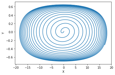
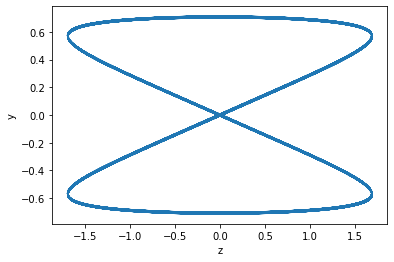
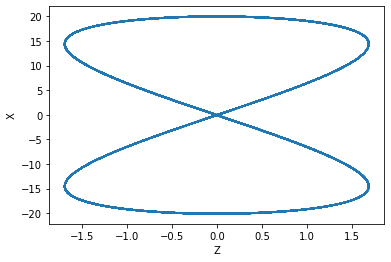
Figure 3: Closer look at particle trajectories in the case of linearly polarized EM wiggler with dominant guide field. The Y-X plane (left panel) illustrates effects of adiabatic switching of the wave: steady state trajectory (outer envelope) is reached on few times for adiabatic switching. The X-Z and Y-Z cuts show trajectories after the steady state is reached. Thinness of the curves composed of multiple tracks illustrate the stability of the codes, and of the adiabatic switching procedure. Largest amplitudes of oscillations are in the wiggler plane $x-z$. Amplitudes of oscillations are not normalized between Fig. 2

(In passing we note that for static wiggler the particle trajectory does depend on the wiggler strength, changing from “vertical 8” to “horizontal 8”, to “circle”: for sufficiently strong wiggler a particle just executes Larmor gyrations, Fig. 4. The latter regimes are not relevant for pulsars.)

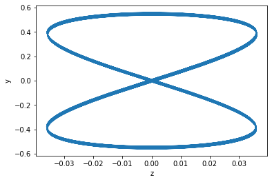
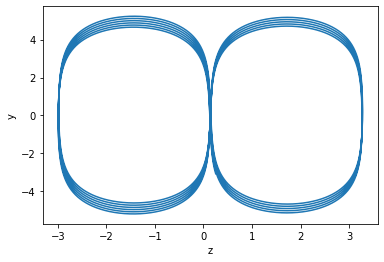
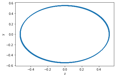
Figure 4: Particles trajectories for strong static wiggler case (no guide field, beam frame). Fixed particle energy, wiggler strength increases left to right. At sufficiently high field (right panel) a particle just executes elliptical Larmor motion within a given field patch. The intermediate case is a curious one: a particle experiences a Spicer-like orbit mostly along the $y$ axis (not along $z$ axis as in the limit of small wiggler field or EM wave, left panel). The strong wiggler regimes (horizontal figure 8 and the ellipse) are not applicable to pulsar magnetospheres.

3.5 Single particle emissivity

3.5.1 Linear regime

Instantaneous and average powers (neglecting terms of the order of $a_{H,b}^{4}$) are

$$W=\frac{2}{3}\left((\alpha-\eta_{g})^{2}\cos^{\xi_{+}}+(1-\alpha\eta_{g})^{2}\sin^{2}{\xi_{+}}\right)\frac{a_{H,b}^{2}e^{2}k_{w,b}^{2}}{c^{3}}\approx\left(1-4\alpha\eta_{g}+\eta_{g}^{2}-(1-\eta_{g}^{2})\right)\frac{a_{H,b}^{2}e^{2}k_{w,b}^{2}}{3c^{3}}\mbox{}$$

$$W_{a}=\left(1-4\alpha\eta_{g}+\eta_{g}^{2}+\alpha^{2}(1+\eta_{g}^{2})\right)\frac{a_{H,b}^{2}e^{2}k_{w,b}^{2}}{c^{3}}\approx\left(1-4\alpha\eta_{g}+\eta_{g}^{2}\right)\frac{a_{H,b}^{2}e^{2}k_{w,b}^{2}}{3c^{3}}$$ (16)

where the last relations neglect $\alpha^{2}$.

Energy flux in the wave

$$S_{w}=(1+\eta_{g}^{2})\frac{B_{0}^{2}}{8\pi}a_{H,b}^{2}$$ (17)

The cross-section

$$\sigma=\frac{W_{a}}{S_{w}}=\frac{8\pi}{3}\left(\frac{1-4\alpha\eta_{g}+\eta_{g}^{2}}{1+\eta_{g}^{2}}\right)\frac{(k_{w,b}c)^{2}}{\omega_{B}^{2}}\frac{e^{4}}{m_{e}^{2}c^{4}}=\left(\frac{1-4\alpha\eta_{g}+\eta_{g}^{2}}{1+\eta_{g}^{2}}\right)\frac{(k_{w,b}c)^{2}}{\omega_{B}^{2}}\sigma_{T}=\mbox{}$$

$$\frac{(k_{w,b}c)^{2}}{\omega_{B}^{2}}\sigma_{T}\times\left\{\begin{array}[]{cc}1,&\mbox{for linearly polarized $\eta_{g}=0$}\\ 1\pm 2\alpha,&\,\mbox{for circularly polarized $\eta_{g}=\pm 1$}\end{array}\right.$$ (20)

Two signs for the circularly polarized wave correspond to two combinations of the wave polarization and direction of rotation of a particle.

For linearly polarized wave, $\eta_{g}=0$ instantaneous acceleration is

$${\bf a}=\{-\sin\xi_{+},\alpha\cos\xi_{+},0\}a_{H,b}k_{w,b}c^{2}$$ (21)

thus, scattered waves are elliptically polarized. In the limit $\alpha\to 0$ the differential cross-section

$$\frac{d\sigma}{d\Omega}=\frac{3}{8\pi}\sigma\sin^{2}\Theta\mbox{}$$

$$\cos\Theta=-\cos\phi\sin\theta$$ (22)

where $\theta,\,\phi$ are the direction of photon propagation. For unpolarized lite

$$\frac{d\sigma}{d\Omega}=\frac{3}{16\pi}\sigma(1+\cos^{2}\theta)$$ (23)

3.6 Non-linear effects: multiple bands

We are interested in the back-scattered X-mode, propagating along the field lines. Using the emission formula

$$\frac{d^{2}I}{d\omega d\Omega}=\frac{e^{2}\omega^{2}}{4\pi^{2}c}[{\bf n}\times({\bf n}\times\tilde{{\bf v}})]^{2}\mbox{}$$

$$\tilde{{\bf v}}=\int dt{\bf v}e^{-i\phi}\mbox{}$$

$$\phi=\omega(t-{\bf n}\cdot{\bf r})\mbox{}$$

$${\bf n}=\{0,0,1\}\mbox{}$$

$$\tilde{{\bf v}}=\int dt\tilde{{\bf v}}_{0}e^{-i\phi}\mbox{}$$

$$\tilde{{\bf v}}_{0}=\{-(1-\alpha\eta_{g}),(\eta_{g}-\alpha f_{w}^{\prime}),0\}\frac{a_{H,b}}{2}\mbox{}$$

$$\phi=(\omega-k_{w,b})t+(\Delta z)(\omega+k_{w,b})\sin 2k_{w,b}t$$ (24)

To take account of the jitter oscillation $(\Delta z)\propto a_{H,b}^{2}$, we use Jacobi-Anger expansion of Bessel functions

$$e^{ib\sin\sigma}=\sum_{n}J_{n}(b)e^{in\sigma}.$$ (25)

We find

$$\tilde{{\bf v}}=\sum_{n}\tilde{{\bf v}}_{0}J_{n}\left((\Delta z)(\omega+k_{w,b})\right)\int dte^{it(\omega-(1+2n)k_{w,b})}$$ (26)

Thus, the resonant condition is

$$\omega=k_{w,b}(1+2n)$$ (27)

A particle produces a set of spontaneous emission bands separated in frequency by $2nk_{w,b}$

The strength of each resonance (Fourier power of velocity) scale as

$$\propto J_{n}\left(\frac{1-\eta_{g}^{2}}{4}(1+n)a_{H,b}^{2}\right)^{2}$$ (28)

Circularly polarized wave, $\eta_{g}=1$ produces only the fundamental mode ($n=0$, $\omega=k_{w,b}$) with scattering cross-section

$$\frac{d^{2}I}{d\omega d\Omega}=(1-\alpha)^{2}\frac{e^{2}\omega^{2}}{4\pi}\delta(\omega-k_{w,b})\mbox{}$$

$$\sigma=(1-\alpha)^{2}\left(\frac{ck_{w,b}}{\omega_{B}}\right)^{2}\left(\frac{e^{2}}{m_{e}c}\right)^{2}$$ (29)

For linearly polarized incoming wave, $\eta_{g}=0$ the strength of each resonance scales as

$$\propto J_{n}\left(\frac{1}{4}(1+n)a_{H,b}^{2}\right)^{2}\approx\frac{(n)^{n}}{2^{2n+1}n!}a_{H,b}^{2n}$$ (30)

The strength of the resonance is determined by the order of the resonance $n$ (for higher $n$ the argument of the Bessel function is larger; this partially compensates the fact that for high $n$ the values of Bessel functions near zero are smaller). Thus, even for small fluctuation of the field $a_{H,b}\ll 1$, higher order resonances may, under certain conditions, become comparable to the basic one.

As a check we performed numerical integration of (24); this, naturally, gives the Jacobi-Anger expansion/resonances, Fig. 5

Figure 5: Numerical Fourier transform of particle’s current (24) with the jitter amplitude $(\Delta z)=0.3$ and $k_{w,b}=1$. Clear resonances are seen at $\omega/k_{w,b}=1+2n$ (this is the direct numerical demonstration of the Jacobi-Anger expansion (25)

3.7 Astrophysical applications of nonlinear scattering: Emission band in Crab’s spectrum

One of the most interesting property of Crab radio emission is observations of numerous emission stripes in Crab High Frequency interpulse (Moffett & Hankins, 1999; Hankins & Eilek, 2007a; Hankins et al., 2016; Eilek & Hankins, 2016). Fig. 1. Emission is composed of at least a dozen relatively narrow emission bands, almost equally spaced in frequency (spacing increases with frequency at a rate of $6\%$). We consider these stripes being the properties of the emission mechanism, not propagation (Lyutikov, 2007). It is one of the most intricate properties of pulsar radio emission - explaining it will be a strong argument in favor of any model of pulsar radio emission.

There is a caveat regarding the band separation in the Crab’s HFIP: the observed stripes in Crab are slightly non-equidistant, band separation increases with observing frequency at a rate of 6% (Hankins et al., 2016; Eilek & Hankins, 2016). We consider this a next-order effect. Most importantly, equal spacing (27) is for single particle emission - non-linear saturation effects may slightly modify the peak frequencies. As a possible route to explain this slight upward shift in frequency separation observed in Crab (Hankins et al., 2016; Eilek & Hankins, 2016), in comparison with regular spacing (27), we offer the following argument. Qualitatively, harmonic wiggler creates periodic variations of the refractive index. The propagation of waves is then described by Hill’s and/or Matthieu’s equation (a parametrically-driven oscillator). For small amplitudes of driving the periodic solutions are separated by a constant frequency difference. At the weakly non-linear stage, the “Floquet tongues” of the Mathieu’s equation (regions of periodic solutions) generally move slightly to higher frequencies. For example, for Mathieu equation written in the form $\ddot{x}+(\omega^{2}+\epsilon\cos(2t))x=0$, $\epsilon\ll 1$, then the center of the second band is located at $<\omega_{2}>=2(1+\epsilon^{2}/192)$ (Casey et al., 1969; Verhulst, 2009). The shift to slightly higher frequency is a general property for harmonic band’s number larger than unity. Thus, nonlinear effects at saturation are expected to shift the band to slightly highly frequencies, as observed. (Beside nonlinearity additional effect that affects the emitted frequency is angle of propagation of the emitted radiation with respect to the structure in the dielectric tensor of the medium, similar to the case of Bragg’s scattering.)

4 Free Electron Laser in guide field dominated regime

4.1 Particle motion in guide-field dominated EM wave and the wiggler

Consider orthogonally polarized harmonic EM modes: wiggler mode with amplitude $a_{H,b}$ (propagating “to the left”) and EM mode with amplitude $a_{EM,b}$ (propagating “to the right”). In the beam frame both waves have the same frequency/wave number $k_{w,b}$. Using parametrization of the vector potential

$${\bf A}=\left(a_{H,b}\{\eta_{g}\sin\xi_{+},\cos\xi_{+},0\}+a_{EM,b}\{\cos\xi_{-},\eta_{EM,b}\sin\xi_{-},0\}\right)\frac{B_{0}}{k_{w,b}}G(t)\mbox{}$$

$${\bf B}={\rm curl\,}{\bf A}+B_{0}{\bf e}_{z}\mbox{}$$

$${\bf E}=-\partial_{t}{\bf A}\mbox{}$$

$$\xi_{-}=k_{w,b}(t-z)\mbox{}$$

$$\xi_{+}=k_{w,b}(t+z)$$ (31)

where $G(t)$ is some switch-on function. Parametrization (31) carries non-zero current components $j_{x,y}\propto\dot{G},\ddot{G}$. Both the adiabatic switch-on terms, and the $\propto 1/\omega_{B}$ terms are needed to get the correct phasing and force-balance.

Average Poynting flux is

$$F_{z}=\left((1+\eta_{EM,b}^{2})a_{EM,b}^{2}-(1+\eta_{g}^{2})a_{H,b}^{2}\right)\frac{B_{0}^{2}}{8\pi}$$ (32)

Assuming non-relativistic motion in the beam frame (so that $1+\beta_{z}\to 1$), neglecting effects of charge separation (this would correspond to the Compton regime of FEL), equations of motion are (switch-on terms are omitted for clarity; full system of equations is used for numerical calculations)

$$\dot{\beta}_{x}=\left(a_{{EM,b}}\sin\left(\xi_{-}\right)-a_{H,b}\eta_{g}\cos\left(\xi_{+}\right)+\beta_{y}\right)\omega_{B}\mbox{}$$

$$\dot{\beta}_{y}=B\left(-a_{{EM,b}}\eta_{{EM,b}}\cos\left(\xi_{-}\right)+a_{H,b}\sin\left(\xi_{+}\right)-\beta_{x}\right)\omega_{B}\mbox{}$$

$$\dot{\beta}_{z}=\left(a_{{EM,b}}\left(\sin\left(\xi_{-}\right)\beta_{x}-\eta_{{EM,b}}\cos\left(\xi_{-}\right)\beta_{y}\right)+a_{H,b}\left(\eta_{g}\cos\left(\xi_{+}\right)\beta_{x}-\sin\left(\xi_{+}\right)\beta_{y}\right)\right)\omega_{B}$$ (33)

Leading terms in $1/{\bf B}_{0}$ expansion give

$$\beta_{x}=\left(\alpha-\eta_{{EM,b}}\right)a_{{EM,b}}\cos\left(\xi_{-}\right)+\left(1+\alpha\eta_{g}\right)a_{H,b}\sin\left(\xi_{+}\right)\mbox{}$$

$$\beta_{y}=-\left(1-\alpha\eta_{{EM,b}}\right)a_{{EM,b}}\sin\left(\xi_{-}\right)+a_{H,b}\left(\alpha+\eta_{g}\right)\cos\left(\xi_{+}\right)\mbox{}$$

$$\dot{\beta}_{z}=\delta\left(\left(1-\eta_{{EM,b}}\eta_{g}\right)\cos\left(2zk_{w,b}\right)-\left(1+\eta_{{EM,b}}\eta_{g}\right)\cos\left(2tk_{w,b}\right)\right)$$ (34)

$$\delta=a_{H,b}a_{EM,b}\omega_{B}$$ (35)

Notice that for $z$-oscillations the leading terms in parameter $\delta$ is ${\cal{O}}(1/B_{0})$ (and not ${\cal{O}}(1/B_{0}^{2})$).

The energy of a particle $\epsilon$ evolve according to

$$\partial_{t}\epsilon=-a_{{EM,b}}a_{H,b}k_{w,b}\left(\eta_{{EM,b}}+\eta_{g}\right)\cos\left(2tk_{w,b}\right)+\frac{1}{2}a_{{EM,b}}^{2}\left(1-\eta_{{EM,b}}^{2}\right)k_{w,b}\sin\left(2\xi_{-}\right)+\frac{1}{2}a_{H,b}^{2}\left(1-\eta_{g}^{2}\right)k_{w,b}\sin\left(2\xi_{+}\right)\propto B_{0}^{-2}$$ (36)

The system (34) is the main set of equations governing particle motion in the combined fields of the wiggler and the EM wave. Qualitatively, the transverse motion is dominated by the electric drift, $\beta_{\perp}\approx{\bf E}\times{\bf B}_{0}/B_{0}^{2}$.

4.2 Dynamics of trapped particles: ponderomotive Hamiltonian

Longitudinal trajectories, Eq. (34), consist of fast jitter $\propto\cos(2k_{w,b}t)$ and slow oscillations $\propto\cos(2k_{w,b}z)$. We can rewrite Eq. (34) as

$$\partial_{t}\left(\frac{\beta_{z}^{2}}{2}+\frac{\delta}{2k_{w,b}}(1-\eta_{EM,b}\eta_{g})\sin(2k_{w,b}z)\right)=-\beta_{z}(1+\eta_{EM,b}\eta_{g})\delta\cos(2k_{w,b}t),$$ (37)

The slow oscillations are governed by

$$\partial_{t}\beta_{z}=\tilde{\delta}\cos(2k_{w,b}z)\mbox{}$$

$$\tilde{\delta}=(1-\eta_{EM,b}\eta_{g})\delta$$ (38)

(Note that only for circularly polarized EM and wiggler $\eta_{EM,b}=\eta_{g}=1$ the slow oscillations vanish.) Below we drop the tilde sign over $\tilde{\delta}$.

Relations (38) allow a first integral

$$\frac{\beta_{z}^{2}}{2}+V_{p}={\rm Const}\mbox{}$$

$$V_{p}=\frac{\delta}{2k_{w,b}}\sin(2k_{w,b}z)$$ (39)

where $V_{p}$ is the ponderomotive potential.

Next we shift the coordinates so that the O-point in $\beta_{z}-z$ plane is at $z=0$ $z\to z-\pi/(4k_{w,b})$, and parametrize the ${\rm Const}$ by the value of the velocity $\beta_{z}=\beta_{0}$ at $z=0$:

$$V_{p}=\frac{\delta}{k_{w,b}}\sin^{2}(k_{w,b}z)$$ (40)

This is the ponderomotive potential. The O-point has $\beta_{z}=\beta_{0}=0$ and is located at $z=0$.

The Hamiltonian then takes the form

$${\cal H}=\frac{\beta_{z}^{2}}{2}+V_{p}=\frac{\beta_{0}^{2}}{2}\mbox{}$$

$$\partial_{t}z=\partial_{\beta_{z}}{\cal H}=\beta_{z}\mbox{}$$

$$\partial_{t}\beta_{z}=-\partial_{z}{\cal H}=-\delta\sin(2k_{w,b}z)$$ (41)

(this is different from (38) due to the $\pi/4$ phase shift). Parameter $\beta_{0}$ is the maximal velocity by a particles in the combined EM-wiggler field.

The separatrix is determined by

$$\beta_{0}=\beta_{S}=\sqrt{2\frac{\delta}{k_{w,b}}}$$ (42)

Normalizing velocities by $\beta_{S}$ the Hamiltonian becomes

$${\cal H}=\beta_{z}^{2}+\sin^{2}(k_{w,b}z)=\eta_{\beta}^{2}\mbox{}$$

$$\beta_{z}=\beta_{z}/\beta_{0,S}\mbox{}$$

$$\eta_{\beta}=\frac{\beta_{0}}{\beta_{0,S}}\leq 1$$ (43)

The flow lines in the $\beta_{z}-z$ plane are then given by

$${\beta_{z}}=\pm\sqrt{\eta_{\beta}^{2}-\sin^{2}(k_{w,b}z)},$$ (44)

Fig. 6. For adiabatic switching, all particles are trapped.

Point where $\beta_{z}=0$ are determined by

$$\sin(k_{w,b}z)=\eta_{\beta}$$ (45)

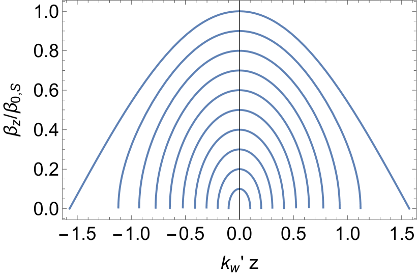
Figure 6: Trajectory of trapped partiles in $\beta_{z}-z$ plane, Eq. (44), $\eta_{\beta}=0.1,\,0.2...0.9.$

In coordinates $\beta_{z}/\beta_{S}-k_{w,b}z$ the X-point is at $45^{\circ}$.

Hamiltonian (41) has an adiabatic invariant

$${\cal I}=\oint\beta_{z}dz=\frac{4\beta_{0}}{k_{w,b}}{\cal E}\left(\arcsin\left(\beta_{0}\frac{k_{w,b}}{2\delta}\right),\frac{2\delta}{k_{w,b}\beta_{0}^{2}}\right)=\frac{4\sqrt{2}\sqrt{\delta}}{k_{w,b}^{3/2}}\eta_{\beta}{\cal E}\left(\arcsin(\eta_{\beta}),1/\eta_{\beta}^{2}\right)$$ (46)

where ${\cal E}$ is the elliptic integral of the second kind.

On the separatrix, $\eta_{\beta}=1$,

$${\cal I}_{S}=\frac{4\sqrt{2}\sqrt{\delta}}{k_{w,b}^{3/2}},$$ (47)

see Fig. 7.

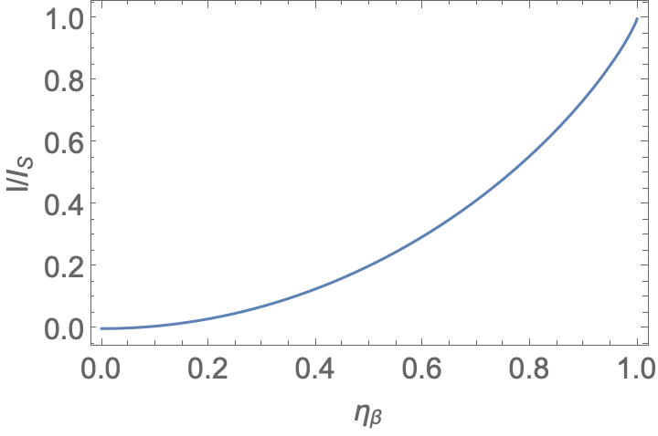
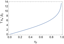
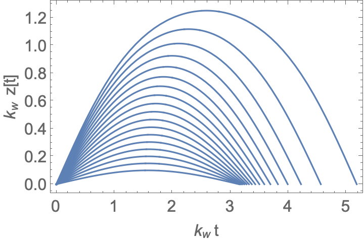
Figure 7: Left Panel: Value of the adiabatic invariant as function of $\eta_{\beta}$. Central Panel: period of oscillations as function of $\eta_{\beta}$ (ratio of maximal velocity along the given trajectory to the maximal velocity on the separatrix). Right Panel: particle trajectories $z(t)$ for different values of $\eta_{\beta}=0.05,\,0.1\,...0.95$.

Motion of a particle can be integrated

$$zk_{w,b}=J_{A}\left(k_{w,b}\beta_{0}t,\frac{1}{\eta_{\beta}^{2}}\right)\mbox{}$$

$$\beta_{z}=\beta_{0}J_{ND}\left(k_{w,b}\beta_{0}t,\frac{1}{\eta_{\beta}^{2}}\right)$$ (48)

where $J_{A}$ is Jacobi amplitude and $J_{ND}$ is Jacobi elliptic function. Time is defined so that at time $t=0$ the particle is at $z=0$.

On the separatrix, $\eta_{\beta}=1$,

$$zk_{w,b}=Gd(k_{w,b}\beta_{0}t)\mbox{}$$

$$\beta_{z}=\beta_{S}{\rm\,sech\,}(k_{w,b}\beta_{S}t)$$ (49)

where $Gd$ is Gudermannian function. Thus, a particle on the separatrix never reaches the point where $\beta_{z}=0$.

A period of oscillations can be found as a (four times) the point where $\beta_{z}$ becomes $0$ in (48), Fig.7.

Slow oscillations are not coherent, in a sense that particles with different parameter $\beta_{0}$ have random phases - thus, density enhancement is approximately constant in time.

4.3 Direct numerical integration of the equation of motion

Equation of motion (35) (with switch-on function re-instated) can be directly integrated. Assuming vanishing initial velocities and employing a switch-on function $G=1-e^{-t/\tau}$, and linearly polarized waves $\eta_{g}=\eta_{EM,b}=0$, particle trajectories, phase diagram and distribution are shown in Fig. 8-9.

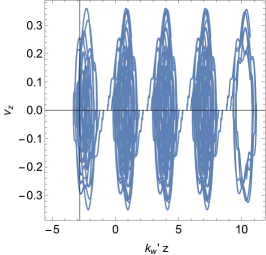
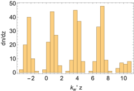
Figure 8: Particle trajectories (left panel), phase diagram (central panel) and distribution (right panel) for particles in counter-propagating wiggler and EM fields (integration of Eq. (34) with initially homogeneous distribution of particles). In this particular example $k_{w,b}=1$, the switch-on function is $G=1-e^{-t/\tau}$ with $\tau=6\pi$, $\delta=0.1$. Particles are initially located at $-\pi<z<3\pi$. Two density enhancements per period are clearly seen (they are constant in time at times much longer than the switch-on time.

Numerical integration clearly shows parametric resonance (Fig. 8, central panel) characteristic of the pendulum equation. O-points (density enhancements) are located at $k_{w,b}z=\pi/4+n\pi$, while X-points are at $k_{w,b}z=3\pi/4+n\pi$ ($n=0,1...$). In case of adiabatic switching all trajectories are trapped (except those starting exactly at the X-points, a set of measure zero). Most importantly, direct numerical integration shows formation of density enhancements near the minimal of the ponderomotive potential.

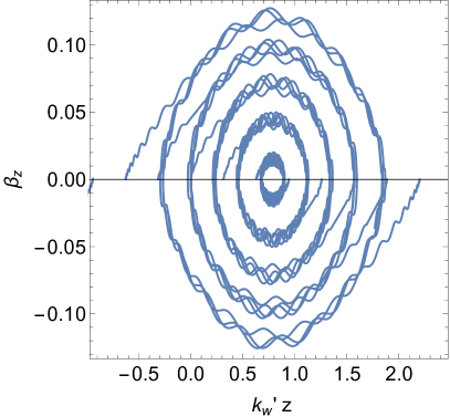
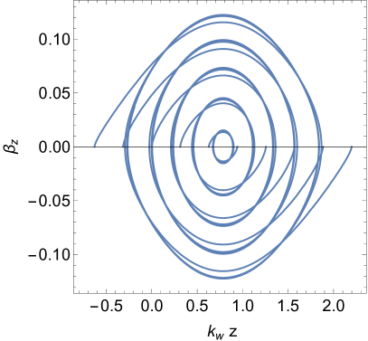
Figure 9: Left panel: Particle trajectories from numerical integration for particles in counter-propagating linearly polarized wiggler and EM fields (integration of Eq. (34) with $\eta_{g}=\eta_{EM,b}=0$.). In this particular example $k_{w,b}=1$, the switch-on function is $G=1-e^{-t/\tau}$ with $\tau=6\pi$, $\delta=0.01$. The motion consists of fast jitter and slow motion around the O-point in the $\beta_{z}-z$ plane. Initial locations of particles are clear seen at the $\beta_{z}=0$ line. Notice how particles are effectively “pulled in” towards the O-point (by the ponderomotive force) - this results in density enhancements. Compare with Fig. 6; only one island is pictured here; location of the O-point is not shifted as in Fig. 44. Right panel: same, but only with the slow term in Eq. (34), $\propto\cos(2k_{w,b}z)$

Charge bunches in the beam are created: Figures 8-9 clearly demonstrate that an initially homogeneous distribution of charges is bunched by the ponderomotive potential.

To provide analytical estimates for the density distribution within a bunch, we note that for a given parameter $\eta_{\beta}$ a probability to find particle at position $z$ is

$$\frac{dp}{dz}\propto\frac{1}{\beta_{z}}$$ (50)

Assuming that initial homogeneous distribution of particles over the phase translates in homogeneous distribution in $\eta_{\beta}$ (this is approximately true, as can be verified by direct numerical integration), integration of Eq. (50) over $0<\eta_{\beta}<$ gives

$$\int_{0}^{1}\frac{dp}{dz}d\eta_{\beta}=\ln\cot(k_{w,b}z/2)\approx\ln\left(\frac{2}{k_{w,b}z}\right)$$ (51)

where the last relation assumes $z\to 0$ (this is a shifted coordinate $z$).

In Fig. 10 we zoom-in into the density distribution within a bunch, showing a nearly 2D charge distribution, consistent with mildly divergent distribution (51)

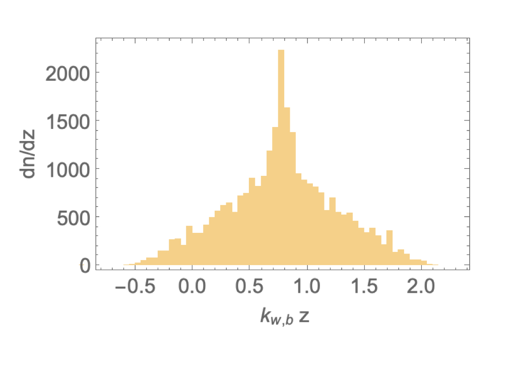
Figure 10: Density distribution within a bunch, averaged over many periods of slow oscillations (arbitrary normalization, random initial phases). The charge distribution is logarithmically divergent, Eq. (51).

4.4 Non-harmonic wiggler

The proposed mechanism works, with some modifications, with non-harmonic wigglers as well. Naturally, the wiggler has to have large power concentrated at the frequencies of the EM to be amplified.

For example, consider Gaussian wiggler pulse(s) propagating to-the-left.

$$B_{w,b}\propto a_{H,b}e^{-(t+z-z_{i})/(2\tau_{G}^{2})}$$ (52)

where $z_{i}$ is the initial position of the wiggler’s peak and $\tau_{G}$ is the duration. Strong effects are expected for short pulses, $\tau_{G}\sim 2\pi/k_{w,b}$, see Fig. 11. Numerical integration clearly shows formation of charge bunches in the wiggler frame.

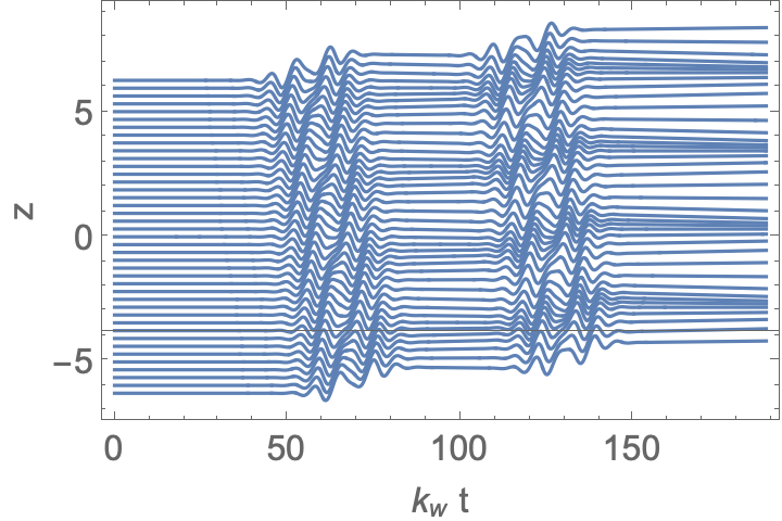
Figure 11: Particle trajectories for two gaussian wigglers located initially at $z_{i,1}=20\pi$ and $z_{i,2}=40\pi$; both wigglers have duration $\tau_{G}=2\pi$. First wiggler creates double density enhancements. The second wiggler both ”shakes” them producing coherent emission, and further amplifies them.

Thus, in a more complicated set-up, non-harmonic wigglers also produce bunches and coherent emission. We expects the effects of charge separation between the wigglers (when there is no ponderomotive force to keep the charges separated), will be modified by plasma oscillations.

Conceptually, a non-harmonic wiggler pulse still creates charge enhancements. After the pulse propagated away, these charge enhancements oscillate electrostatically, so that the following wiggler pulse propagates through Langmuir turbulence, shaking the charged density enhancements and producing coherent emission.

4.5 Comparison with unmagnetized case

Let us next compare cases of static wigglers with no guide field and guide-field dominated case. Let in the frame of the wiggler the fluctuating field be $B_{w}$ and wavelength $k_{w}$. In this frame a particle is moving with Lorentz factor $\gamma_{0}$. (The case of electromagnetic and static wigglers are nearly equivalent for $\gamma_{0}\gg 1$, hence we use the same notations for the static wiggler.)

A particle executes a trajectory with longitudinal radius of curvature

$$R_{c}\sim\frac{1}{a_{H}k_{w}}$$ (53)

It is much larger than the size of the transverse circle a particle makes, which for circular polarized wiggler is $r_{g}\sim a_{H}/k_{w}$.

Single particle emissivities (neglecting factors of the order of unity and effects of wiggler polarization.)

$$P_{\rm no-B}\approx\frac{e^{2}}{c}\gamma_{b}^{2}\omega_{B_{w}}^{2}\mbox{}$$

$$P_{\rm B}\approx\frac{e^{2}}{c}a_{H}^{2}\gamma_{b}^{4}(k_{w}c)^{2}\mbox{}$$

$$\frac{P_{\rm B}}{P_{\rm no-B}}=\left(\gamma_{b}\frac{k_{w}c}{\omega_{B}}\right)^{2}\ll 1\mbox{}$$

$$\omega_{B_{w}}=\frac{eB_{w}}{m_{e}c}$$ (54)

The total power $P_{\rm B}$ obeys the Larmor formula for curvature emission, but the spectrum is different: Landau-Pomeranchuk effects are dominant. For a particle with Lorentz factor $\gamma$ the radiation formation length is (Landau & Lifshitz, 1975)

$$l_{c}\sim\gamma^{2}\frac{c}{\omega}\sim 1/k_{w}$$ (55)

(relativistic electron separates by a wavelength from own radiation for a time $\gamma^{2}$ times wave period.) Thus, within a radiation formation length the particle changes its velocity considerably. As a result, the emission is of Compton type, $\omega\sim\gamma_{b}^{2}k_{w}c$, not curvature (where we would have expected $\omega\sim\gamma_{b}^{3}{a_{H}k_{w}}c$).

In case of single particle motion, many relations for the guide-field dominated case can be recovered with a change

$$K_{u}\equiv\frac{eB_{w}}{m_{e}c^{2}k_{w}}\rightarrow a_{H,b}\gamma_{b}$$ (56)

where $K_{u}$ is the conventional undulator parameter.

4.6 Plasma effects in the beam and the background

The wiggler produces density fluctuation. These fluctuation of charge density will produce electrostatic field that will affect beam dynamics. We consider them next.

The particles move due to both electrostatic electric field $E_{z}=-\partial_{z}\Phi$ ($\Phi$ is the electrostatic potential) and the Lorentz force. Using relations (35) for linearly polarized waves $\eta_{g}=\eta_{EM,b}=0$, and adding electrostatic acceleration (in the non-relativistic regime $\beta_{z}\ll 1$), the axial equation of motion becomes

$$\partial_{t}\beta_{z}=\partial_{z}\Phi+\delta\left(\cos\left(2zk_{w,b}\right)-\cos\left(2tk_{w,b}\right)\right)$$ (57)

Using charge conservation

$$\partial_{t}\delta n+\partial_{z}\left(\beta_{z}(n_{0}+\delta n)\right)=0,$$ (58)

and Poisson equation

$$\Delta\Phi=4\pi e\delta n,$$ (59)

the system (57-59) represent a closed set for charge density, electrostatic potential and velocity field.

Treating density fluctuations $\delta n$ and $\beta_{z}^{\prime}$ as small quantities, we find

$$\beta_{z}=-\delta\frac{2k_{w,b}}{(2k_{w,b})^{2}-\omega_{p,b}^{2}}\sin(2k_{w,b}t)\mbox{}$$

$$\omega_{p,b}^{2}=\frac{4\pi e^{2}n_{b}}{m_{e}}$$ (60)

where $n_{b}$ is beam density in its frame.

Relation (60) clearly demonstrates a resonance between Langmuir oscillations and wiggler-induced jitter. The resonance occurs when the double frequency of the wiggler (recall that the wiggler produces longitudinal oscillations at its double frequency) matches the plasma frequency.

Importantly, under the corresponding approximation of small amplitude of jitter motion, the phase of the density oscillations is not affected, only the amplitude. The two regimes have a name in the field of FEL research: (i) Compton regime $\omega_{p,b}\ll k_{w,b}c$; (ii) Raman regime $\omega_{p,b}\gg k_{w,b}c$. As we discuss in §6.2, in astrophysical setting the scattering may occur in either regime.

In conclusion, while the amplitude of oscillations due to the ponderomotive driving depends on the beam plasma frequency, its phase is not. Thus plasma effects in the beam affect the strength of driving, but not the resonance condition.

We leave numerical consideration of electrostatic effects in the beam to a future paper. The approach to follow electrostatic oscillation in quasi one-dimensional approach for charged beams has been previously outlined by Levinson et al. (2005); Timokhin (2010).

Presence of background plasma may affect operation of FEL in several ways: (i) plasma dispersion is modified, hence waves are not vacuum waves; (ii) wave escape: emission should be either produced on a mode that evolves into vacuum mode and escapes directly, or should be converted into escaping waves; (iii) background plasma may compensate the charges bunches in the beam.

Let us address these issues in turn. Obliquely propagating modes in pulsar magnetospheres, at frequencies below the cyclotron frequency, can be separation in the X-mode (with electric field perpendicular to the ${\bf B}-{\bf k}$ plane) (Arons & Barnard, 1986; Kazbegi et al., 1991; Lyutikov, 1998; Keppens et al., 2019). For parallel propagation we are left only with X-mode with near-vacuum dispersion

$$\omega_{X}\approx kc\left(1-\frac{\omega_{p,bulk}^{2}}{\omega_{B}^{2}}\right)$$ (61)

where $\omega_{p,bulk}$ is the bulk (background) plasma density. In magnetically dominated plasma $\omega_{p,bulk}/\omega_{B}\ll 1$ the X-mode is nearly a vacuum mode.

Most importantly, the X-mode extends continuously from $\omega\leq\omega_{p,b}$ to $\omega\geq\omega_{p,b}$ (e.g. , Figure 2 in Lyutikov, 2007). It does not suffer plasma/Landau absorption at $\omega\sim\omega_{p,b}$. X-mode is escaping mode: as plasma density decreases, it connects to the vacuum mode.

We leave consideration of possible effects of the background plasma on the charge separation in the beam to a subsequent paper. Here we just note that though background’s plasma density is higher than that of the beam, in the beam frame the background’s plasma dynamics will be suppressed by $\sim\gamma_{b}^{-3/2}$.

5 Generation of coherent emission

5.1 Growth rate of parametric instability

Qualitatively, the period of slow oscillations (in the beam frame)

$$\tau_{s}\sim\frac{1}{k_{w,b}\beta_{S}}=\frac{1}{\sqrt{k_{w,b}\delta}}=\frac{1}{\sqrt{a_{EM,b}a_{H,b}}}\frac{1}{\sqrt{k_{w,b}\omega_{B}}}\mbox{}$$

$$\tau_{s}\times(k_{w,b}c)=\left(\frac{1}{a_{H,b}a_{EM,b}}\right)^{1/2}\left(\frac{k_{w,b}c}{\omega_{B}}\right)^{1/2}$$ (62)

This is also a time to develop charge bunches.

The evolution (growth) of the amplitude of the electromagnetic wave occurs on similar time scale. Qualitatively its evolution is then governed by

$$\partial_{t}a_{EM,b}=\frac{a_{EM,b}}{\tau_{s}}=\sqrt{a_{H,b}k_{w,b}\omega_{B}}a_{EM,b}^{3/2}$$ (63)

with a solution

$$\frac{a_{EM,b}}{a_{EM,0}}=\frac{1}{(1-t\Gamma_{b})^{2}}\mbox{}$$

$$\Gamma_{b}={\sqrt{a_{H,b}a_{EM,0}}}{\sqrt{k_{w,b}c\omega_{B}}}/2$$ (64)

where $a_{EM,0}$ is the initial amplitude of the EM wave.

Eq. (64) gives the growth rate for parametric instability (micro-bunching) due to the interaction of wiggler field with normalized amplitude $a_{H,b}$ and the electromagnetic field with initial amplitude $a_{EM,0}$ (both measured in the beam frame). Relation (64) shows two important points: (i) instability is explosive, reaching infinite amplitude in finite time; (ii) growth rate is determined by the initial value of the EM wave intensity $a_{EM,0}$. Note that the growth rate is only mildly suppressed by the guiding magnetic field, $\Gamma_{b}\propto B_{0}^{-1/2}$.

5.2 Growth rate in the high-gain/SASE regime

Growth rate of the parametric instability (64) depends on the initial amplitude of the electromagneticwave $a_{EM,0}$. What determines $a_{EM,0}$? It is most likely determined by an external seed radiation. As a lower limit, we can use an analogues of SASE (Self-Amplified Spontaneous Emission) regime of FEL, where micro-bunching is initiated by the spontaneous radiation.

Let us estimate how much spontaneous emission is generated by plasma particles within a “lethargy” region $\sim r$ (measured in lab frame). In the beam frame the corresponding size is $\gamma_{b}r$. In the beam frame the Poynting flux of a wiggler is

$$F_{w}=a_{H,b}^{2}\frac{B_{0}^{2}}{4\pi}c$$ (65)

The scattered flux from a layer of thickness of $\gamma_{b}r$ is then

$$F_{scat}=n_{b}\sigma_{M}\gamma_{b}rF_{w}\mbox{}$$

$$\sigma_{M}=\left(\frac{k_{w,b}c}{\omega_{B}}\right)^{2}\sigma_{T}=4\gamma_{b}^{2}\left(\frac{k_{w}c}{\omega_{B}}\right)^{2}\sigma_{T}$$ (66)

where $\sigma_{M}$ is magnetic cross-section for X-mode and $\sigma_{T}$ is Thomson cross-section, $n_{b}$ is the beam density in the beam’s frame. Equating scattered flux $F_{scat}$ to the initial EM flux,

$$F_{scat}=a_{EM,0}^{2}\frac{B_{0}^{2}}{4\pi}c$$ (67)

we find

$$a_{EM,0}=\sqrt{r\gamma_{b}n_{b}\sigma_{T}}a_{H,b}\alpha$$ (68)

(recall: $\alpha=k_{w,b}c/\omega_{B}$). We find for temporal growth rate

$$\Gamma_{b}\approx\left(rn_{b}\sigma_{T}{\gamma_{b}}\right)^{1/4}{{a_{H,b}}}(k_{w,b}c)$$ (69)

In the observer frame

$$\Gamma=\frac{\Gamma_{b}}{\gamma_{b}}=\left(rn_{b}\sigma_{T}\right)^{1/4}\frac{{a_{H}}}{{\gamma_{b}}}\omega\mbox{}$$

$$\omega=2\gamma_{b}ck_{w,b}=4\gamma_{b}^{2}(ck_{w})\mbox{}$$

$$a_{H,b}=\gamma_{b}a_{H}\mbox{}$$

$$n=\gamma_{b}n_{b}$$ (70)

Spacial growth length is $L_{w}\sim c/\Gamma$. We can then define the magnetic Pierce parameter $\rho_{B}$ as

$$\rho_{B}=\frac{1/k_{w}}{L_{w}}=a_{H}\left(\gamma_{b}^{2}\frac{J}{I_{A}}\frac{r_{e}}{k_{w}}\right)^{1/4}\mbox{}$$

$$J=nec\mbox{}$$

$$r_{e}=\frac{e^{2}}{m_{e}c^{2}}\mbox{}$$

$$I_{A}=\frac{m_{e}c^{3}}{e}$$ (71)

(dimensionless factors have been omitted in the definition of $\rho_{B}$). Different scaling of $\rho_{B}$ from the conventional Pierce parameter can be traced to magnetic cross-section (66).

5.3 Saturation of the parametric instability

Calculations of the non-linear saturation levels of coherent instabilities is a daunting task. It requires calculations of how non-linear back reaction from the emitted wave affects that particle distribution, and the condition when that back-reaction saturations. Any order-of-magnitude estimate should be taken with a grain of salt.

As a physically motivated assumption, we suggest the following criteria for the saturation level. The instability is a parametric excitation of EM waves. As the amplitude of EM waves growth (parameter $\delta$, Eq (35), the energy of the motion of the trapped particles increases. The saturation will be reached, we assume, when the energy density of the motion of the trapped particles (of the initially cold beam) approaches the energy density of the EM waves (in the beam frame).

The ponderomotive potential (40), with parameter $\delta$ increases linearly with EM wave intensity $a_{EM,b}$, while energy density of EM waves increases quadratically $\propto a_{EM^{2}}$. The balance is achieved at

$$m_{e}n_{b}\frac{\beta_{S}^{2}}{2}=a_{EM,b}^{2}\frac{B_{0}^{2}}{4\pi}\to\frac{a_{EM,b}}{a_{H,b}}=\frac{\omega_{p,b}^{2}}{k_{w,b}c\omega_{B}}$$ (72)

where typical velocity of trapped particles $\beta_{S}$ is given by (75). This is an estimate of he saturation level of the EM waves in the beam frame.

In the observer frame this gives

$$\frac{a_{EM}}{a_{H}}={2}{\gamma}^{2}\frac{\omega_{p}^{2}}{\omega\omega_{B}}$$ (73)

Or, in terms of conversion efficiency of the beam’s energy into radiation $\eta_{b-r}$ ,

$$\eta_{b-r}\equiv\frac{B_{EM}^{2}/(4\pi)}{n\gamma m_{e}c^{2}}=4\gamma^{3}a_{H}^{4}\frac{\omega_{p}^{2}}{\omega^{2}}$$ (74)

(see Eq. (94) for numerical estimates in astrophysical applications.)

The corresponding saturated velocity jitter

$$\beta_{0,Sat}=\sqrt{2}a_{H,b}\frac{\omega_{p,b}}{k_{w,b}}=\frac{a_{H}}{\sqrt{2\gamma}}\frac{\omega_{p}}{k_{w}c}$$ (75)

This is also an estimate of the applicability of the cold beam approximation. If the velocity spread in the beam is larger that (75), then the parametric instability is suppressed. As we discuss in §B, the velocity spread in the beam frame is much smaller than in the observer frame, so the constant (75) is not very strict. Also, in astrophysical applications we expect ${\omega_{p,b}}\sim{k_{w,b}}$, §6.2.

5.4 Simple emissivity model of a charged bunch

As a simple estimate we can assume that particles within each half a period are bunched into a charged layer. This charged layer is shaken by the wiggler and emits coherently. The surface charge density for each layer is

$$\sigma_{e}=en_{b}\frac{\pi}{k_{w,b}}=en\frac{\pi}{k_{w}},$$ (76)

it oscillates with velocity $a_{H,b}c$ in its frame. Using jump conditions for oscillating fields on the oscillating charged layer, the resulting Poynting flux and energy density of radiation are

$$P_{b}=2\pi a_{H,b}^{2}\sigma_{e}^{2}=2\pi^{3}e^{2}c\frac{n^{2}}{k_{w,b}^{2}}a_{H,b}^{2}\mbox{}$$

$$\epsilon_{b}=\frac{P}{c}$$ (77)

(this is the value on each side of a charged layer - total energy loss is two times larger).

In the lab frame

$$P=P_{b}\gamma_{b}^{2}=2\pi^{3}\gamma_{b}^{4}\frac{e^{2}c^{3}n^{2}}{\omega^{2}}a_{H}^{2}=\frac{\pi^{3}}{8}\frac{e^{2}cn^{2}}{k_{w,b}^{2}}a_{H}^{2}$$ (78)

Scaling $\propto n^{2}$ clearly indicates a coherent process.

5.5 Constructive interference from different bunches

The intensity for parallel propagating emitted electromagnetic wave is given by (Jackson, 1999, Eq. 14.70)

$$\frac{d^{2}I}{d\omega d\Omega}=\frac{\omega^{2}}{4\pi^{2}c^{3}}\left|{\cal S}\right|^{2}\mbox{}$$

$${\cal S}\propto\sum_{m}\int dt\int dzj_{x}e^{i\omega(t-z_{m})}$$ (79)

where the sum is over the location of the charges. Neglecting axial oscillations.

$$\int dz\beta_{x}=(-1)^{m+1}\frac{1}{\sqrt{2}}\left((a_{EM,b}-a_{H,b})\cos(k_{w,b}t)+(a_{EM,b}+a_{H,b})\sin(k_{w,b}t)\right)\approx(-1)^{m}a_{H,b}\cos(\pi/4+k_{w,b}t)$$ (80)

where in the last relation we neglected $a_{EM,b}\ll a_{H,b}$. Thus, emission from different charged layers adds constructively, Fig. 12

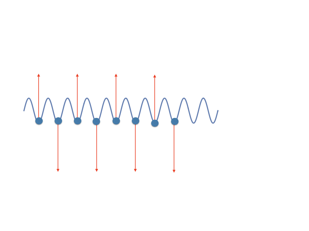
Figure 12: Constructive addition of emission from different charged bunches. Wiggled curve represent the ponderomotive potential. Particles are bunched at the minima of the potential creating charged bunches (solid circles). Bunches are shaken by the wiggler (red arrows). By the time an electromagnetic wave from a give bunch arrives at the location of a neighboring one, the velocity reverses, so that waves add constructively.

Thus, within the simple emission model, each layer emits coherently, and emission from different layers add constructively.

6 Astrophysical viability

6.1 Plasma parameters in pulsars and magnetars

The suggested mechanism of coherent radio production depends on two ingredients: the wiggler and the reconnection-generated beam. In Lyutikov (2020a) we discussed properties of firehose-excited wigglers, and in §A we discuss properties of Alfvén (low frequency) wigglers. Next we consider the expected properties of the particle beam and astrophysical applications, concentrating on Alfvén wigglers (scaling $k_{w,b}$ to the local radius, not the plasma properties).

Two scalings for the plasma density of the beam are viable: the pulsar-like (Goldreich & Julian, 1969) and magnetar-like (Thompson et al., 2002). As we expect the FEL to operate both in pulsars (Crab) and magnetars/FRBs, we consider both cases in parallel.

Let’s assume that radio emission is generated at distance $r$, and typical wiggler wavelength is related to $r$, but is somewhat smaller,

$$k_{w}=\eta_{w}\frac{2\pi}{r},\,\eta_{w}\geq 1$$ (81)

For a beam of Lorentz factor $\gamma_{b}$ the emitted frequency is

$$\omega\sim 8\pi\eta_{w}\gamma_{b}^{2}\frac{c}{r}$$ (82)

The required Lorentz factor is

$$\gamma_{b}=\eta_{w}^{-1/2}\left(\frac{\nu r}{4c}\right)^{1/2}=\left\{\begin{array}[]{c}10^{2}\,\eta_{w}^{-1/2}\left(\frac{r}{R_{NS}}\right)^{1/2}\nu_{9}^{1/2}\\ 10^{3}\,\eta_{w}^{-1/2}\left(\frac{r}{R_{LC}}\right)^{1/2}\nu_{9}^{1/2}\end{array}\right.$$ (83)

where for two estimates the radius is normalized to the neutron star radius (top row) and Crab’s light cylinder radius (bottom row).

Both estimates are very reasonable: such Lorentz factor are indeed expected both in magnetar magnetospheres (Beloborodov & Thompson, 2007; Cerutti & Beloborodov, 2017) and in the reconnection current sheets in Crab pulsar (Zenitani & Hoshino, 2007; Cerutti et al., 2015b; Contopoulos, 2016). Thus, even the longest wiggler, with the wavelength of the order of the distance to the star, can reasonably produce GHz radio emission with relatively mild, by pulsar standards, Lorentz factors.

6.2 Density estimates: Crab and magnetars

For magnetars, as an estimate of the beam density (in lab frame) we can use

$$n=(\Delta\phi)\frac{B}{4\pi er}$$ (84)

where $(\Delta\phi)$ is twist angle of magnetospheric field lines (Thompson et al., 2002). Using Lorentz transformation to the beam frame,

$$k_{w,b}=2\gamma_{b}k_{w}\mbox{}$$

$$n_{b}=\frac{n}{\gamma_{b}}$$ (85)

we find the ratio of beam plasma frequency to the wiggler frequency (in the beam frame)

$$\frac{\omega_{p,b}}{ck_{w,b}}\approx\left\{\begin{array}[]{c}10^{4}\times b_{q}^{1/2}(\Delta\phi)^{1/2}\eta_{w}^{-1/4}\left(\frac{r}{R_{NS}}\right)^{-7/4}\nu_{9}^{-3/4}\\ 3\times\left(\frac{b_{q}}{0.1}\right)^{1/2}(\Delta\phi)^{1/2}\eta_{w}^{-1/4}\left(\frac{r}{R_{LC}}\right)^{-7/4}\nu_{9}^{-3/4}P_{0.03}^{-7/4}\\ \end{array}\right.$$ (86)

(For Crab $b_{q}\approx 0.1$.) Though the factor in (86) is large, $\sim 10-10^{4}$, all the parameters are smaller than unity, $b_{q}^{1/2},\,(\Delta\phi)^{1/2},\,\eta_{w}^{-1/4},\,\left({r}/{R_{NS}}\right)^{-7/4}\leq 1$. Thus, wiggler-plasma resonance effects (§4.6) can be important (so that density bunching is enhanced).

Alternatively, scaling beam density to the Goldreich & Julian (1969) density

$$n_{GJ}=\frac{\Omega B}{2\pi ec}\mbox{}$$

$$\frac{\omega_{p,b}}{ck_{w,b}^{\prime}}\approx\left\{\begin{array}[]{c}10^{4}\times b_{q}^{1/2}\eta_{w}^{-1/4}\left(\frac{r}{R_{NS}}\right)^{-5/4}\nu_{9}^{-3/4}P_{0.03}^{-1/2}\\ 3\times\left(\frac{b_{q}}{0.1}\right)^{1/2}\eta_{w}^{-1/4}\left(\frac{r}{R_{LC}}\right)^{-5/4}\nu_{9}^{-3/4}P_{0.03}^{-7/4}\end{array}\right.$$ (89)

where neutron star period is scaled to Crab.

This is a very important result: we find that in magnetars perturbation of the magnetosphere  with scales somewhat smaller that the size of a neutron star, as well as in Crab pulsar perturbation of the magnetosphere  with scales somewhat smaller that the light cylinder, are likely to produce oscillation of the beam plasma in resonance with the charge oscillations in the beam. In magnetars the required Lorentz factor is $\gamma\sim 10^{2}$, in Crab $\gamma\sim 10^{3}$: all reasonable estimates.

Possibility of wiggler-beam plasma resonance adds further complication. Resonant interaction enhances bunching, but it depends sensitively on the properties of the driver and the dissipation processes; less so on the power of the driver.

6.3 Growth rate: Crab pulsar and magnetars

Relation (70) give the growth rate of the parametric (bunching) instability. For astrophysical applications we chose two cases: Crab pulsar and magnetars, §6.2.

Parametrizing wiggler wavelength by (81), the condition

$$\frac{\Gamma}{c/r}\geq 1$$ (90)

requires

$$\eta_{w}^{1/2}a_{H}\geq\left(\frac{c^{2}}{n\sigma_{T}\omega^{2}r^{3}}\right)^{1/4}$$ (91)

This is a condition on the amplitude of the wiggler $a_{H}$ and its typical length $r/\eta_{w}$, so that in the SASE regime the spacial growth rate is larger than the distance to the star.

Using density parameterizations of §6.2, the condition (91) then gives

$$\eta_{w}^{1/2}a_{H}\geq 6\times 10^{-3}b_{q}^{-1/4}\nu_{9}^{-1/2}(\Delta\phi)^{-1/4}(r/R_{NS})^{-1/2}\,\mbox{for magnetars}\mbox{}$$

$$\eta_{w}^{1/2}a_{H}\geq 3\times 10^{-2}\nu_{9}^{-1/2}\,\mbox{for Crab},$$ (92)

Thus, in both cases mild wiggler intensity $a_{H}\geq 10^{-3}$ is needed (recall that $\eta_{w}\geq 1$, Eq. (81)).

6.4 Expected brightness temperature

Estimating/calculating the power of coherent sources - in astrophysical setting when no lab technician is on-site - is, in some sense, a treacherous road. Coherence depends on the subtle addition of phases of emitted wave; the saturation levels depend on non-linear back-reaction of coherently added waves on the kinetic properties of the distribution function.

There are two ingredients for the production of radiation: the wiggler and the beam. Comparing the expected energy densities in the beam and the wiggler

$$\frac{\gamma nm_{e}c^{2}}{a_{H}^{2}B_{0}^{2}/(8\pi)}=\left\{\begin{array}[]{c}10^{-14}\times b_{q}^{-1}a_{H}^{-2}\eta_{w}^{-1/2}\left(\frac{r}{R_{NS}}\right)^{5/2}\nu_{9}^{1/2}\\ 6\times 10^{-9}\times b_{q}^{-1}a_{H}^{-2}\eta_{w}^{-1/2}\left(\frac{r}{R_{LC}}\right)^{7/2}\nu_{9}^{1/2}P_{0.03}^{5/2}\end{array}\right.$$ (93)

for magnetar and pulsar scalings. This demonstrates that beam energy density is typically much lower than that of the wiggler: the beam cannot smooth out the wiggler field. We conclude that for typically the energy density of wiggler’s turbulence is much higher than that of the beam. It is then the energy of the beam that determines the resulting radiation: energy in the wiggler is not a limiting factor.

The beam-radiation conversion efficiency (74) evaluates to

$$\eta_{b-r}=a_{H}^{4}\gamma_{3}^{3}\nu_{9}^{-2}\times\left\{\begin{array}[]{cc}5\times 10^{4}&\mbox{Crab}\\ 10^{15}\,b_{q}(\Delta\phi)\left(\frac{r}{R_{NS}}\right)&\mbox{magnetars}\end{array}\right.$$ (94)

Values of $\eta_{b-r}$ are both highly dependent on the amplitude of the wiggler $\propto a_{H}^{4}$, and have large numerical factors. This implies, first, that ver weak wigglers, with $a_{H}\ll 1$ are sufficient to convert a faction of the beam energy into radiation, and, second, that this conversion efficiency is almost a threshold effect.

The resulting brightness temperature is (Lyutikov & Rafat, 2019)

$${k_{B}{T}_{b}}=\eta_{b-r}(2\gamma)^{4}\frac{\lambda^{3}m_{e}c^{2}n}{2\pi}$$ (95)

where $\lambda=c/\nu$ is wavelength.

Using two parameterizations for plasma density, we find

$$T_{b}=\eta_{b-r}\times\gamma_{3}^{4}\nu_{9}^{-3}\left\{\begin{array}[]{cc}10^{43}{\rm K}\,\,\,b_{q}(\Delta\phi)\left(\frac{r}{R_{NS}}\right)^{-1}&\mbox{magnetars}\\ 2\times 10^{33}{\rm K}&\mbox{Crab}\par\end{array}\right.$$ (96)

for magnetar and G-J scaling correspondingly.

Somewhat surprisingly (given the order-of-magnitude estimates) the brightness temperature estimates (96) match both the FRBs and Crab GPs (Manchester & Taylor, 1977; Melrose, 2000; Soglasnov et al., 2004; Lorimer et al., 2007; Petroff et al., 2019). We consider this a major, and unexpected, success of the model.

6.5 Energetics

Finally, let us comment on the energetics of FRBs. In the case of FRBs the energetics is constrained by the accompanying X-ray bursts $E_{X}$ (not the FRB itself). The required size $l_{M}$ of a region of dissipated magnetic energy is

$$l_{M}\sim 2\pi^{1/3}\frac{E_{X}^{1/3}}{B_{NS}^{2/3}}=5\times 10^{4}{\rm cm}b_{q}^{-2/3}E_{X,40}^{1/3}$$ (97)

about a football field for the quantum critical surface magnetic field. Time-alignment of few msec between radio and X-rays imply then that radio emission in FRBs is also generated relatively close to the NS’s surface, at $r\leq 10^{8}$ cm.

7 Advantages of guide-field dominate wiggler

In the present astrophysical application guide-field dominates linear wiggler has a number of advantages. First, In laboratory FEL linearly polarized wigglers produce ${\bf B}_{0}\times\nabla\delta{\bf B}$ drift that causes the beam to drift away and expand. This is a fatal problem in the lab because the beam blows up. The guide field suppresses drifts, Fig. 13.

Most importantly, guide field dominance helps to maintain beam coherence, Fig. 13.b. Without the guide field particles with different energies follow different trajectories, and quickly lose coherence even for small initial velocity spread. In contrast, in the guide-field dominated regime all particles follow, basically, the same trajectory. Hence coherence is maintained as long as the velocity spread in the beam frame is $\Delta\beta\leq 1$.

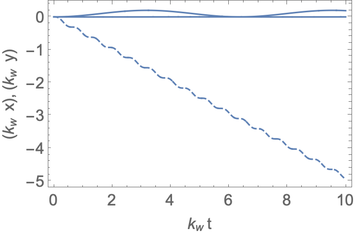
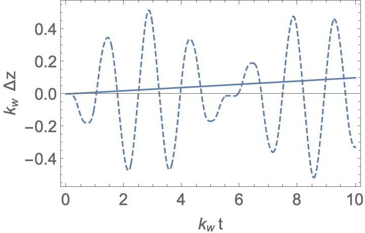
Figure 13: Comparison of cross-field drift and phase separation in wigglers without guide and in the guide field dominated regime, static wigglers. Left pane: cross-field displacement for guide-field dominated wiggler $a_{H,b}=10$ (solid line) and no guide field (dashed lines for x and y) as a function of time. Right panel: axial separation $\Delta$ of two particles with initial velocities $\beta_{1}=0.98$ and $\beta_{2}=0.99$. In the guide field dominated regime phase coherence is much better preserved.

8 Discussion

We construct a model of coherent radio emission generation in pulsars, magnetars and Fast Radio Bursts. We suggest that radio emission in all these cases is reconnection-powered. In the case of Crab Giant Pulses, the reconnection events occur outside the light cylinder in the magnetic equator current sheet, while in the case of magnetars and FRBs it occurs deep inside the neutron star magnetospheres.

The emission mechanism is a variant of Free Electron Laser. In neutron star’s magnetospheres the FEL operates in a guide-field dominated regime, $\omega_{B}\gg\gamma_{b}k_{w}c$. This is highly unusual regime by laboratory standards.

Reconnection events launch fast particle beams propagating along magnetic field  perturbed either by the pre-existing or self-generated turbulence. The turbulence may be driven either by magnetohydrodynamical effects, or by the firehose/two stream instability of counter-propagating plasma components. Turbulent fluctuations (the wiggler) create charge bunches in the beam (via ponderomotive force) that coherently scatter the wiggler field.

The present model explains a number of fairly subtle features of radio emission in Crab, magnetars and FBRs:

• conforms with the predicted nearly simultaneous observations of radio and X-rays burst in magnetars, with radio slightly ahead of the X-rays (Mereghetti et al., 2020), as predicted by Lyutikov (2003, 2017).

• operates in a very broad range of neutron star’s parameters: the model is independent of the value of the magnetic field. It is thus applicable to a broad variety of NSs, from fast spin/weak magnetic field millisecond pulsars to slow spin/super-critical magnetic field in magnetars, and from regions near the surface up to (and a bit beyond of) the light cylinder.

• the model require only mildly narrow distribution of beam’s particles, $\Delta p/p_{0}\leq 1$ and the spectrum of turbulence $\Delta k_{w,b}/k_{w,b}\leq 1$

• reproduces (multiple) emission bands seen in Crab and FRBs; the model also can produce broader spectrum emission.

• matches the polarization properties of FRBs (those that show narrow emission bands are linearly polarized, while broad-band emission can be circularly polarized)

• naturally gives correct estimates for the brightness temperatures both in pulsars and FRBs.

• The model is also consistent with overall duration of FRBs, from microseconds to milliseconds (Nimmo et al., 2020): the dissipation size needed for a medium X-ray flare accompanying an FRB is $\sim 100$ meters $=10^{-2}$ of the radius; hence FRB, emitting along B-field it might last $\sim 10^{-2}$ of the period - milliseconds, if the source works long enough. But FRB can be as short as light crossing time over 100 meters, a microsecond.

We hypothesize that the radio emission is generated during the initial stage of magnetospheric reconnection, while the magnetosphere is still relatively clean of the pair loading. The giant $\gamma$-ray flare from the magnetar SGR 1806 - 20 had a rise time of only $200$ micro-seconds (Palmer et al., 2005), matching the duration of the radio flare. In a possibly related study of relativistic reconnection by Lyutikov et al. (2017a, b, 2018), it was found that in highly magnetized plasma the reconnection process driven by large scale stresses (magnetically-driven collapse of an X-point) has an initial stage of extremely fast acceleration, yet low level of magnetic energy dissipation. This initial stage of reconnection may produce unstable particle distribution in the yet clean surrounding, not polluted by pair production.

Other points of importance include:

• Radio emission is generated during the initial stages of magnetospheric reconnection, as argued by (Lyutikov, 2003; Lyutikov & Lorimer, 2016). Lyutikov et al. (2017a, b, 2018) found that in highly magnetized plasma the reconnection process driven by large scale stresses (magnetically-driven collapse of an X-point) has an initial stage of extremely fast acceleration, yet low level of magnetic energy dissipation. Observations of Mereghetti et al. (2020) confirm that radio leads high energy.

• FRB duration and intrinsic time structure is determined by the lateral (not radial) extension/structure of the emission (Lyutikov, 2020c). Roughly speaking, if both the wiggler and the particle beam have extension $\sim R_{NS}$, the effective radial direction of the generated pulse would be $\sim c/(R_{NS}\gamma_{b}^{2})$ - much shorter than the observed duration of an FRB. (In passing we note that the closest analogue - Solar type-III bursts - also sometimes show fine spectral structure, classified as type-IIIb (stria) bursts Ellis & McCulloch, 1967, we think FRBs’ fine structure is different in origin.).

• Large magnetic fields at the FRB production cites are required, otherwise coherently emitting particles will have dominant “normal” (synchrotron and inverse Compton) losses Lyutikov (2017); Lyutikov & Rafat (2019). In high magnetic field instead of large oscillations with momentum $p_{\perp}\sim a_{A}m_{e}c$, the coherently emitting particles experience mild $E\times B$ drift.

• The high energy and radio burst from SGR 1935+2154 lies not far from the so-called Güdel-Benz relationship, which relates the thermalized X-ray luminosity generated by magnetic reconnection in stellar flares to the nonthermal, incoherent, gyrosynchrotron radio emission. Güdel-Benz correlation is usually interpreted that first electrons are accelerated to non-thermal velocities and emit radio, then these particles are thermalized and emit thermal X-rays. The magnetar SGR 1935+2154 adds another point, with an important caveat that the radio emission in this case is coherent. (Interestingly, it also lies off to the “expected” side from the lower energetics fit: the radio is too bright, as expected for coherent emission.) Though the microphysics of this relation is far from clear, is it at least consistent with the concept that accelerating mechanism puts first energy into nonthermal particles that produce radio, and then that energy is thermalized, producing X-rays.

A number of principal issues need to be addressed:

• reconnection and particle in magnetically dominated plasmas has been recently extensively studies (e.g.  Lyutikov & Uzdensky, 2003; Lyutikov, 2003; Lyubarsky, 2005; Uzdensky, 2011; Uzdensky & Spitkovsky, 2014; Guo et al., 2015; Lyutikov et al., 2017a, b, 2018; Werner & Uzdensky, 2017). Acceleration in relativistic reconnection is complicated. It depends on the details of plasma components and the value of the guide field (e.g. competition of tearing mode and drift kink modes Lyutikov, 2003; Komissarov et al., 2007; Zenitani & Hoshino, 2007, 2008; Sironi & Spitkovsky, 2014; Sironi et al., 2016), as well as large scale properties of the magnetic configurations (Lyutikov et al., 2017a, b, 2018). What is missing so far is similar studies in highly radiatively-dominated regime of magnetars.

• The model relates magnetar/FRB emission to a particular type of pulsar radio emission, associated with Crab GPs. Only few pulsars show a phenomenon of GP (Staelin & Reifenstein, 1968; Romani & Johnston, 2001; Johnston & Romani, 2003; Soglasnov et al., 2004; Kuzmin, 2007). Why only few pulsars show GPs?

• In case of Crab, effects of cyclotron resonance need to be investigated further (it is not realistic in magnetars, see §3.1). Near the cyclotron resonance interaction of the beam particles with the wiggler/EM wave can be very efficient since the resonant scattering cross-section is huge (1996ASSL..204.....Z; 2006MNRAS.368..690L). This increases the efficiency of wiggler-beam coupling. Effects of radiative damping should be taken into account:

  $$\tau_{b}\approx\frac{m_{e}c^{3}}{e^{2}\omega_{B}^{2}}\mbox{}$$

  $$\tau=\gamma_{b}\tau_{b}\mbox{}$$

  $$\frac{\tau\Omega}{2\pi}\approx 1\times\gamma_{3}$$ (98)

  where $\tau_{b}$ is the cyclotron decay time in beam frame, $\tau$ is in the lab frame, and the numerical estimate is for Crab pulsar near the light cylinder. Thus, effects of radiative damping, even at Crab’s light cylinder, may prevent operation of relativistic cyclotron masers (where masing occurs due to orbital bunching of electrons 1974ApPhL..25..377S; 1995PhRvE..52..998N).

• Plasma effects in the beam. The wiggler produces density fluctuation. These fluctuation of charge density will produce electrostatic field that will affect beam dynamics. In the present approach we considered what is called the Compton regime of FEL - neglecting beam plasma effects. This requires that wiggler/EM frequency (in the beam frame) is much larger than that the plasma frequency of the beam. In the opposite regime (Raman) the scattering in done not by a simple particles, but by plasma oscillations. It is expected that the amplitude of oscillations due to the ponderomotive driving depends on the beam plasma frequency, but its phase does not. Thus plasma effects in the beam affect the strength of driving, but not the resonance condition. We leave numerical consideration of electrostatic effects in the beam to a future paper. The approach to follow electrostatic oscillation in quasi one-dimensional approach for charged beams has been previously outlined by Levinson et al. (2005); Timokhin (2010).

• What are the effects of the background plasma? Presence of background plasma may affect operation of FEL in several ways: (i) plasma dispersion is modified, hence waves are not vacuum waves; (ii) wave escape: emission should be either produced on a mode that evolves into vacuum mode and escapes directly, or should be converted into escaping waves; (iii) background plasma may compensate the charges bunches in the beam. We leave consideration of possible effects of the background plasma on the charge separation in the beam to a subsequent paper. Here we just note that though background’s plasma density is higher than that of the beam, in the beam frame the background’s plasma dynamics will be suppressed by $\sim\gamma_{b}^{-3/2}$.

• Angular spreading and resulting coherence degradation. Since wiggles are non-relativistic the coherence conditions are not affected by transverse wiggling. Internal beam spreading, effects of “emittance” using laboratory FEL terminology, are better studies in full PIC simulations.

• In the case of FRBs, it is not clear why repeaters typically show narrow emission bands with linear polarization, while (apparent) non-repeaters are broadband with more varies polarization properties (Petroff et al., 2019).

In conclusion, we developed a conceptually new model for the generation of coherent emission in pulsars (Crab in particular), magnetars and FRBs. The emission is not rotationally, but reconnection-driven. A combination of analytical and (fairly basic) numerical results explain a surprisingly wide range of phenomena (e.g. emission stripe(s), brightness temperatures and polarization correlations), the model is fairly robust to wiggler/beam parameters (requires only mildly narrow distributions) and is independent of the value of the magnetic field (hence applicable to a broad range of astrophysical objects). We encourage more detailed analysis, especially using PIC simulations.

We would like to thank Roger Blandford, Samuel Gralla, Igor Kostyukov, Henry Freund, Amir Levinson, Mikhail Medvedev, Alexander Philippov, Sergey Ryzhkov, Anatoly Spitkovsky. Python code was written by Yegor Lyutikov. We also thank him for comments on the manuscript. This work was initiated while ML was a graduate student at Caltech; discussions with Peter Goldreich are acknowledged.

This work had been supported by NASA grants 80NSSC17K0757 and 80NSSC20K0910, NSF grants 1903332 and 1908590.

Appendix A Alfvén force-free solitons

As we discussed above, for highly relativistic particle the difference between a static wiggler and a propagating EM packet of Alfvén waves is minimal (for analysis of linear waves in pulsar magnetospheres see Arons & Barnard, 1986; Lyutikov, 1998; Keppens et al., 2019). Two types of wigglers/ Alfvén waves can be produced in the magnetospheres of neutron stars. First, large scale magnetospheric motions, associated with (pre-)flare global evolution of magnetic fields may/will generate Alfvén waves with the typical wavenumber related to the local radius $r$, $k_{w,b}\sim\eta_{w}(1/r)$, $\eta_{w}\geq 1$. Second, development of current driven instabilities, of the firehose-type, can lead to generation of Alfvén waves (Lyutikov, 2020a, also, Lyutikov & Philippov, in prep.). In both cases we expect Alfvenic perturbations propagating in the magnetosphere. In the present Chapter we consider properties of the nonlinear modes in the pulsar magnetosphere(force-free modes have been considered by Thompson & Blaes, 1998; Gruzinov, 1999; Komissarov, 2002; Pfeiffer & MacFadyen, 2013; Lyutikov, 2011; Gralla & Jacobson, 2014, 2015)

A.1 Light darts

Gralla & Jacobson (2015) found a number of solution for nonlinear force-free perturbations. Here we extend their solutions to the problem of wiggler fields in pulsar magnetospheres. Consider force-free plasma in magnetic field of value $B_{0}$ directed along the $z$-axis, subject to an electromagnetic perturbation. First, consider perturbation in Cartesian coordinates,

$${\bf A}=\left(A_{x}(x,y,\xi_{+}){\bf e}_{x}+A_{y}(x,y,\xi_{+}){\bf e}_{y}+A_{z}(x,y,\xi_{+}){\bf e}_{z}\right)\mbox{}$$

$${\xi_{+}}=k_{z}z-\omega t$$ (A1)

Ideal condition then requires $A_{z}=0$.

Two remaining modes can be separated. The transverse components of the vector potential can be separated into curl-free (“O-modes”) and div-free “X-modes” components.

For “O-modes” the transverse vector potential is a gradient of a function

$${\bf A}_{\perp}=\nabla_{2}\Phi(x,y)=\partial_{x}\Phi(x,y){\bf e}_{x}+\partial_{y}\Phi(x,y){\bf e}_{y}\mbox{}$$

$$\omega=k_{z}\mbox{}$$

$$j_{z}=k_{z}^{2}\Delta_{2}\partial_{{\xi_{+}}}\Phi(x,y,\xi_{+})\mbox{}$$

$$\nabla_{2}=\{\partial_{x},\partial_{y}\}\mbox{}$$

$$\Delta_{2}=\partial_{x}^{2}+\partial_{y}^{2}$$ (A2)

The force-free equations are satisfied for arbitrary $\Phi(x,y)$. These are “light darts” (Gralla & Jacobson, 2015). They are fully nonlinear solutions of force-free equations. (Importantly, $j_{z}$ is a linear function of $\Phi$. In particular, if $\Delta_{2}\Phi=0$, there is no current and the perturbation becomes vacuum-like. In cartesian coordinates harmonic 2D functions are divergent (e.g.  $\propto\cos(k_{1}x)\cosh(k_{1}y)$), but this property will allow us to find new non-linear solution in cylindrical geometry, Eq. (A7).

Thus, O-modes (as well as TEM modes in cylindrical geometry) could be called force-free Alfvén wave. They carry energy only along $z$-axis. For example, for harmonic $\Phi(x,y)\propto e^{i(k_{x}x+k_{y}y)}$ the Poynting flux averaged over a period is $\propto(k_{x}^{2}+k_{y}^{2})k_{z}^{2}{\bf e}_{z}$.

Second, there is a set of “X-modes”, where the vector potential is

$${\bf A}_{\perp}=\nabla_{2}\Psi(x,y,\xi_{+})\times{\bf e_{z}}=\partial_{y}\Psi(x,y,\xi_{+}){\bf e}_{x}-\partial_{x}\Psi(x,y,\xi_{+}){\bf e}_{y}$$ (A3)

This is just a vacuum X-mode, ${\bf J}=0$.

Let us generalize previous relations to cylindrical coordinates, with perturbations of the type

$${\bf A}=\left(A_{TEM}(r,k_{z}z-\omega t){\bf e}_{r}+A_{TE}(r,k_{z}z-\omega t){\bf e}_{\phi}+A_{TM}(r,k_{z}z-\omega t){\bf e}_{z}\right)e^{im\phi}$$ (A4)

(using the standard notation for cylindrical wave-guide modes: Transverse Magnetic (TM), Transverse Electric (TE) and Transverse electromagnetic wave (TEM) modes.

In vacuum, radial and $k_{z}z-\omega t$ dependance is separable, while $k_{z}z-\omega t$ dependance is naturally required to be harmonic. Propagating modes with $\omega\neq 0$ then require: (i) TEM mode requires $m=0$, $\omega=k_{z}$, $A_{TEM}\propto 1/r$ (one needs a cylindrical surfaces such as a coaxial cable to support a TEM wave); (ii) TE mode requires $m=0$, $A_{TE}=J_{1}\left(\sqrt{\omega^{2}-k_{z}^{2}}r\right)$; TM mode requires $k_{z}=0$, $A_{TM}=J_{m}(r\omega)$;

In force-free, the ideal condition requires that the TM mode must have $\omega=0$, $k_{z}=0$, $A_{TM}\propto r^{\pm m}$: only static, $z$-independent and limited in radius solution. Transverse Magnetic waves do not exist in force-free plasma.

For the TEM mode, we find that for $m=0$ and $\omega=k_{z}$ any solution is fully non-linear with arbitrary $A_{TEM}\left[(r,k_{z}(\omega-t)\right]$.

$${\bf A}_{TEM}=A_{TEM}(r,k_{z}(z-t){\bf e}_{r},\,m=0$$ (A5)

(”Light darts” are not limited to axially-symmetric perturbations, as discussed above in Cartesian coordinates.)

TEM mode carries non-zero axial current (cf. , (A2))

$$J_{z,TEM}=\frac{k_{z}\partial_{r}\partial_{\xi_{+}}\left(rA_{TEM}(r,\xi_{+})\right)}{r}\equiv k_{z}\partial_{\xi_{+}}(\nabla_{2}\cdot{\bf A}_{TEM})$$ (A6)

Finally

$${\bf A}_{TE}=J_{1}(r\sqrt{\omega^{2}-k_{z}^{2}})e^{i(k_{z}z-\omega t)}{\bf e}_{\phi}$$ (A7)

The mode ${\bf A}_{TE}$ is the vacuum TE mode, that has no associated current or charge. It satisfied the condition $\nabla_{2}\cdot{\bf A}_{TE}$. It is a axisymmetric analogue of the harmonic X-mode.

(Regarding the terminology, we can these solutions solitons, but they are not, in a conventional sense - balance between dispersion and nonlinearity - these are soliton-looking fully nonlinear solutions.)

To summarize, in the present treatment, there is an interesting correspondence: in vacuum there are two modes, TM and TE; the TEM mode is discarded since it is divergent on the axis. In force free, TE mode remains, since it has zero current, TM mode is discarded, and - somewhat surprisingly - the TEM mode is not divergent.

A.2 Properties of force-free solitons

The mode ${\bf A}_{TEM}$ describes an axially-symmetric EM perturbation, that can be limited both in $z-t$ and $r$, an Alfvén soliton. For example, choosing (similar procedure can be repeated in Cartesian coordinates giving “Alfvén sheets”)

$$A_{TEM}=B_{w}re^{-(r/r_{0})^{2}}e^{-\xi_{+}^{2}}\mbox{}$$

$${\xi_{-}}=k_{z}(z-t)$$ (A8)

($d_{w}$ is a $z$-scale of soliton in terms of $2\pi/k_{z}$) we find fields and currents, see Fig.

$${\bf B}=-{2{\xi_{+}}(k_{z}r)e^{-{{\xi_{+}}^{2}}-\frac{r^{2}}{r_{0}^{2}}}}B_{w}{\bf e}_{\phi}+B_{0}{\bf e}_{z}\mbox{}$$

$$E_{r}=B_{\phi}\mbox{}$$

$${\bf J}=-{4{\xi_{+}}}\left(1-\frac{r^{2}}{r_{0}^{2}}\right)B_{w}k_{z}e^{-{{\xi_{+}}^{2}}-\frac{r^{2}}{r_{0}^{2}}}{\bf e}_{z}\mbox{}$$

$$\rho=J_{z}\mbox{}$$

$${\bf B}\cdot{\bf E}=0\mbox{}$$

$$B^{2}-E^{2}=B_{0}^{2}\geq 0$$ (A9)

At every point the four-current is null, $|\rho|=|j|$.

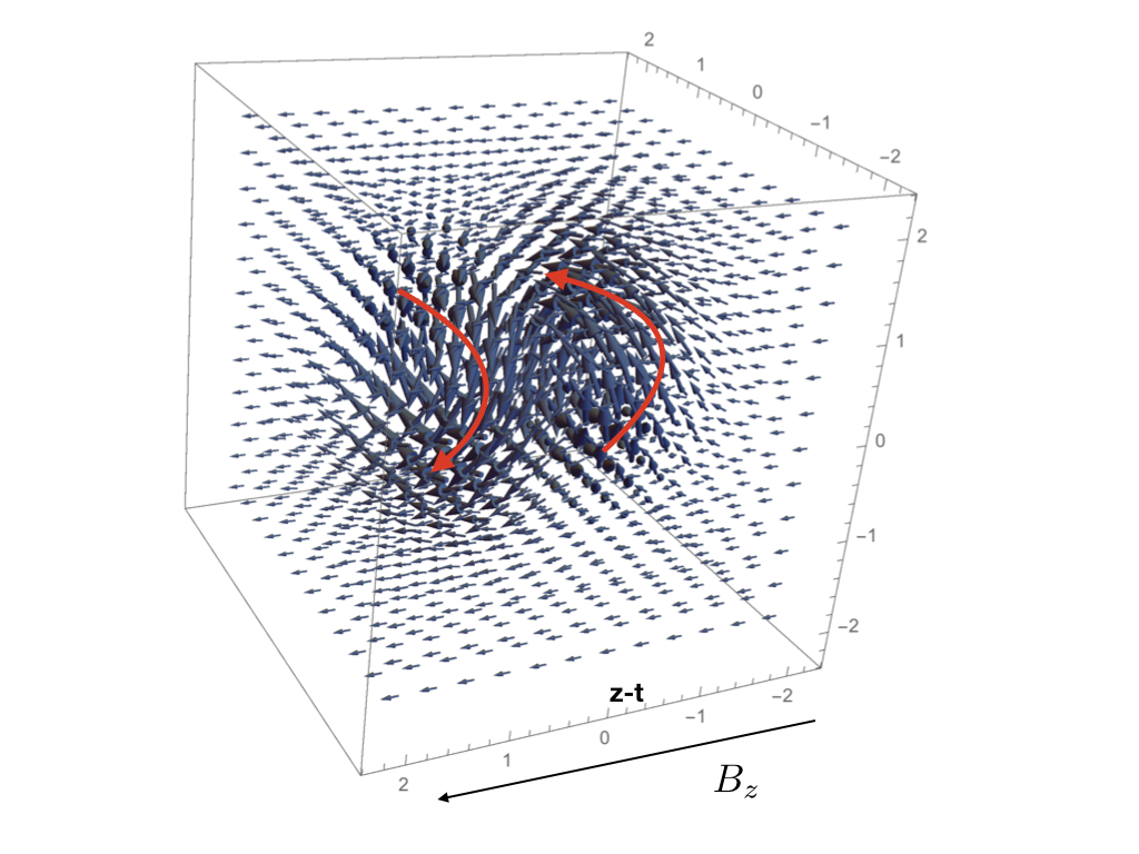
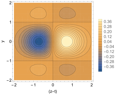
Figure 14: Left Panel: 3D rendering of magnetic field in a non-linear force-free Alfvén soliton, Eq. (A9). Amplitude of soliton-related magnetic field  perturbations is exaggerated for clarity. Right Panel: Charge density (slice in the $(z-t)-y$ plane). The EM fields of the soliton are limited in both transverse and longitudinal direction (double Gaussian).

Electromagnetic velocity (this is a drift velocity across magnetic field)

$$\frac{{\bf E}\times{\bf B}}{B^{2}}=2\left({\xi_{+}}k_{z}ra_{H,b}e^{-\left({\xi_{+}}^{2}+\frac{r^{2}}{r_{0}^{2}}\right)}{\bf e}_{\phi}+2{\xi_{+}}^{2}(k_{z}r)^{2}a_{H,b}^{2}e^{-2\left({\xi_{+}}^{2}+\frac{r^{2}}{r_{0}^{2}}\right)}{\bf e}_{z}\right)\left(1+4{\xi_{+}}^{2}(rk_{z})^{2}a_{H,b}^{2}e^{-2\left({\xi_{+}}^{2}+\frac{r^{2}}{r_{0}^{2}}\right)}\right)^{-1}\approx\mbox{}$$

$$2{\xi_{+}}k_{z}ra_{H,b}e^{-\left({\xi_{+}}^{2}+\frac{r^{2}}{r_{0}^{2}}\right)}{\bf e}_{\phi}+4{\xi_{+}}^{2}(k_{z}r)^{2}a_{H,b}^{2}e^{-2\left({\xi_{+}}^{2}+\frac{r^{2}}{r_{0}^{2}}\right)}{\bf e}_{z}$$ (A10)

where $a_{H,b}=\delta B/B_{0}$ (in lab frame - this is different from the notation in the main paper.) As the soliton propagates, it induces plasma rotation that changes sign in the middle, plus plasma motion along the $z$-direction. At $r\leq r_{0}$ the plasma rotates with nearly constant angular velocity. Another curious property of the solution is that the radial component of ${\rm curl\,}{\bf B}$ is exactly cancelled by $\partial_{t}{\bf E}$.

The total charge carried by the soliton is zero. It is due to the cancellation of two pair of charges, at ${\xi_{+}}>,<0$ and $r>,<r_{0}$, Each of the total value $\pm(2\pi/e^{1})B_{w}r_{0}^{2}$. Thus, the solution carries typical charge density

$$\rho_{s}\approx\frac{B_{w}k_{z}}{{2\pi}}$$ (A11)

Comparing charge density (A11) to the GJ density $\rho_{GJ}$, and a density expected in magnetospheres of magnetars

$$\frac{\rho_{s}}{\rho_{GJ}}\approx{a_{H,b}}({k_{z}R_{LC}})\approx\frac{a_{H,b}}{\gamma_{b}^{2}}\frac{R_{LC}}{\lambda}\mbox{}$$

$$\frac{\rho_{s}}{{(\Delta\phi)}B_{0}/r}=\frac{a_{H,b}}{{(\Delta\phi)}}k_{z}r\approx\frac{a_{H,b}}{{(\Delta\phi)\gamma_{b}^{2}}}\frac{r}{\lambda}$$ (A12)

where in the latter relations we used $\omega\sim c/\lambda\sim\gamma_{b}^{2}k_{w,b}c$.

Since the background plasma is expected to have total plasma density larger than the minimal one by a factor $\kappa\sim 10^{3}$, conditions of charge starvation are

$$a_{H,b}\leq\gamma_{b}^{2}\kappa\frac{\lambda}{R_{LC}}=7\gamma_{0,3}^{3}\kappa_{3}\mbox{}$$

$$a_{H,b}\leq\gamma_{b}^{2}\kappa(\Delta\phi)\frac{\lambda}{r}=10^{3}\gamma_{0,3}^{3}\kappa_{3}(\Delta\phi)$$ (A13)

for emission at $\lambda=1$ cm. Thus, charge starvation is not likely to affect Alfven solitons.

Appendix B Momentum spread of the beam

Here we demonstrate that (i) a mild spread of particle momenta in the observer frame, $\Delta p/p\leq 1$ is sufficient to keep coherence; (ii) mild “normal” radiative losses (non-coherent) help greatly in reducing the momentum spread of the particles.

B.1 Relativistic kinematic reduction of thermal spread of the beam

Let’s assume a fast beam propagates with Lorentz factor $\gamma_{b}$ and has thermal spread $\theta$ in its rest frame. Juttner-Maxwell distribution for the beam in the observer frame is

$$f(p)=\frac{1}{2\theta\gamma_{b}K_{1}(1/\theta)}e^{-(\gamma\gamma_{b}-pp_{b})/\theta}\mbox{}$$

$$\gamma=\sqrt{p^{2}+1}\mbox{}$$

$$p_{b}=\sqrt{\gamma_{b}^{2}-1}\mbox{}$$

$$\int fdp=1$$ (B1)

Assuming $1\ll\theta\leq\gamma_{b}$,

$$f=0.24\frac{1}{\theta\Gamma K_{1}(1/\theta)}e^{-(\gamma-\gamma_{b})^{2}/(2\gamma_{b}^{2}\theta)}$$ (B2)

The spread in the momentum (and the Lorentz factor) of the beam in the observer frame is $\Delta\gamma\approx\gamma_{b}^{2}\theta$. Inversely, a spread in the center of momentum frame of the beam is $\theta=(\Delta\gamma_{b}/\gamma_{b})/\gamma_{b}\ll(\Delta\gamma_{b}/\gamma_{b})$.

Thus, for any relativistic beam with $\gamma_{b}\gg 1$, if the relative energy spread in the observer frame is $(\Delta\gamma/\gamma_{b})\leq 1$, then the corresponding spread in the frame of the beam becomes tiny $\ll 1$.

B.2 Reduction of thermal spread due to cooling

Particles accelerated at reconnection will experience cooling via synchrotron, IC and curvature emission. As discussed by Lyutikov et al. (1999) for curvature emission this will lead to drastic reduction in the spread of the Lorentz factors in the beam frame. Generally, if cooling scales as

$$\partial\gamma=-c_{1}\gamma^{1+\alpha}$$ (B3)

($\alpha=1$ for IC and synchrotron cooling and $\alpha=3$ for curvature), the energy of each particle evolves according to

$$\frac{\gamma(t)}{\gamma_{b}}=\left(1+c_{1}\alpha\gamma_{b}^{\alpha}t\right)^{-1/\alpha}$$ (B4)

Integrating along trajectories we find that a spread in Lorentz factors evolves according to

$$\frac{\Delta\gamma}{\Delta\gamma_{b}}=\left(\frac{\gamma_{b}(t)}{\gamma_{b}}\right)^{2(1+\alpha)}\mbox{}$$

$$\frac{\Delta\gamma}{\gamma_{b}(t)}=\left(\frac{\gamma_{b}(t)}{\gamma_{b}}\right)^{1+2\alpha}\frac{\Delta\gamma_{b}}{\gamma_{b}}$$ (B5)

where $\gamma_{b}(t)$ is the average Lorentz factor at time $t$. Overall cooling of the beam by a factor of 2 reduces its Lorentz factor spread by a factor $2^{1+2\alpha}=8,\,128$ for $\alpha=1,3$. Thus, mild overall cooling of the beam particles results in drastic reduction of the internal spread of Lorentz factors.

References

- Akhiezer et al. (1975) Akhiezer, A. I., Akhiezer, I. A., Polovin, R. V., Sitenko, A. G., & Stepanov, K. N. 1975, Oxford Pergamon Press International Series on Natural Philosophy, 1
- Alferov et al. (1989) Alferov, D. F., Bashmakov, Y. A., & Cherenkov, P. A. 1989, Soviet Physics Uspekhi, 32, 200
- Arons (2012) Arons, J. 2012, Space Sci. Rev., 173, 341
- Arons & Barnard (1986) Arons, J., & Barnard, J. J. 1986, ApJ, 302, 120
- Arons & Scharlemann (1979) Arons, J., & Scharlemann, E. T. 1979, ApJ, 231, 854
- Bai & Spitkovsky (2010) Bai, X.-N., & Spitkovsky, A. 2010, ApJ, 715, 1282
- Beloborodov & Thompson (2007) Beloborodov, A. M., & Thompson, C. 2007, ApJ, 657, 967
- Beskin (2018) Beskin, V. S. 2018, Physics Uspekhi, 61, 353
- Beskin et al. (1988) Beskin, V. S., Gurevich, A. V., & Istomin, I. N. 1988, Ap&SS, 146, 205
- Bespalov & Trakhtengerts (1986) Bespalov, P. A., & Trakhtengerts, V. Y. 1986, Alfvenic masers, in Russian (Gorky: IPF AN USSR)
- Birdsall & Langdon (1991) Birdsall, C. K., & Langdon, A. B. 1991, Plasma Physics via Computer Simulation
- Bochenek et al. (2020) Bochenek, C. D., Ravi, V., Belov, K. V., et al. 2020, Nature, 587, 59
- Camilo et al. (2006) Camilo, F., Ransom, S. M., Halpern, J. P., et al. 2006, Nature, 442, 892
- Casey et al. (1969) Casey, K. F., Matthes, J. R., & Yeh, C. 1969, Journal of Mathematical Physics, 10, 891
- Cerutti & Beloborodov (2017) Cerutti, B., & Beloborodov, A. M. 2017, Space Sci. Rev., 207, 111
- Cerutti et al. (2015a) Cerutti, B., Philippov, A., Parfrey, K., & Spitkovsky, A. 2015a, MNRAS, 448, 606
- Cerutti et al. (2015b) —. 2015b, MNRAS, 448, 606
- Cerutti et al. (2016) Cerutti, B., Philippov, A. A., & Spitkovsky, A. 2016, MNRAS, 457, 2401
- Chen & Beloborodov (2014) Chen, A. Y., & Beloborodov, A. M. 2014, ApJ, 795, L22
- Cheng & Ruderman (1977) Cheng, A. F., & Ruderman, M. A. 1977, ApJ, 216, 865
- CHIME/FRB Collaboration et al. (2020) CHIME/FRB Collaboration, Andersen, B. C., Bandura, K. M., et al. 2020, Nature, 587, 54
- Chime/Frb Collaboration et al. (2020) Chime/Frb Collaboration, Amiri, M., Andersen, B. C., et al. 2020, Nature, 582, 351
- Cohen et al. (1991) Cohen, B. I., Cohen, R. H., Nevins, W. M., & Rognlien, T. D. 1991, Reviews of Modern Physics, 63, 949
- Colson (1976) Colson, W. B. 1976, Physics Letters A, 59, 187
- Connor et al. (2016) Connor, L., Sievers, J., & Pen, U.-L. 2016, MNRAS, 458, L19
- Contopoulos (2016) Contopoulos, I. 2016, Journal of Plasma Physics, 82, 635820303
- Contopoulos & Stefanou (2019) Contopoulos, I., & Stefanou, P. 2019, MNRAS, 487, 952
- Cordes & Chatterjee (2019) Cordes, J. M., & Chatterjee, S. 2019, ARA&A, 57, 417
- Cordes & Wasserman (2016) Cordes, J. M., & Wasserman, I. 2016, MNRAS, 457, 232
- Deacon et al. (1977) Deacon, D. A. G., Elias, L. R., Madey, J. M. J., et al. 1977, Phys. Rev. Lett., 38, 892
- Eilek & Hankins (2016) Eilek, J. A., & Hankins, T. H. 2016, Journal of Plasma Physics, 82, 635820302
- Ellis & McCulloch (1967) Ellis, G. R. A., & McCulloch, P. M. 1967, Australian Journal of Physics, 20, 583
- Fawley et al. (1977) Fawley, W. M., Arons, J., & Scharlemann, E. T. 1977, ApJ, 217, 227
- Freund & Antonsen (1986) Freund, P. H., & Antonsen, M. T. 1986, Principles of Free-electron Lasers
- Friedland (1980) Friedland, L. 1980, Physics of Fluids, 23, 2376
- Ginzburg & Peskov (2013) Ginzburg, N. S., & Peskov, N. Y. 2013, Physical Review Accelerators and Beams, 16, 090701
- Ginzburg (1947) Ginzburg, V. 1947, Izv. Acad.Sci. USSR, Physics, 11, 165
- Goldreich & Julian (1969) Goldreich, P., & Julian, W. H. 1969, ApJ, 157, 869
- Goldreich & Keeley (1971) Goldreich, P., & Keeley, D. A. 1971, ApJ, 170, 463
- Gralla & Jacobson (2014) Gralla, S. E., & Jacobson, T. 2014, MNRAS, 445, 2500
- Gralla & Jacobson (2015) —. 2015, Phys. Rev. D, 92, 043002
- Gruzinov (1999) Gruzinov, A. 1999, ArXiv Astrophysics e-prints
- Guo et al. (2015) Guo, F., Liu, Y.-H., Daughton, W., & Li, H. 2015, ApJ, 806, 167
- Hankins & Eilek (2007a) Hankins, T. H., & Eilek, J. A. 2007a, ApJ, 670, 693
- Hankins & Eilek (2007b) —. 2007b, ApJ, 670, 693
- Hankins et al. (2016) Hankins, T. H., Eilek, J. A., & Jones, G. 2016, ApJ, 833, 47
- Hessels et al. (2019) Hessels, J. W. T., Spitler, L. G., Seymour, A. D., et al. 2019, ApJ, 876, L23
- Hibschman & Arons (2001) Hibschman, J. A., & Arons, J. 2001, ApJ, 560, 871
- Istomin (2004) Istomin, Y. N. 2004, in IAU Symposium, Vol. 218, Young Neutron Stars and Their Environments, ed. F. Camilo & B. M. Gaensler, 369–+
- Jackson (1999) Jackson, J. D. 1999, Classical Electrodynamics: Third Edition (John Wiley & Sons, Inc.)
- Johnston & Romani (2003) Johnston, S., & Romani, R. W. 2003, ApJ, 590, L95
- Josephy et al. (2019) Josephy, A., Chawla, P., Fonseca, E., et al. 2019, arXiv e-prints, arXiv:1906.11305
- Kazbegi et al. (1991) Kazbegi, A. Z., Machabeli, G. Z., Melikidze, G. I., & Smirnova, T. V. 1991, Astrophysics, 34, 234
- Kennel & Pellat (1976) Kennel, C. F., & Pellat, R. 1976, Journal of Plasma Physics, 15, 335
- Keppens et al. (2019) Keppens, R., Goedbloed, H., & Durrive, J.-B. 2019, Journal of Plasma Physics, 85, 905850408
- Komissarov (2002) Komissarov, S. S. 2002, MNRAS, 336, 759
- Komissarov et al. (2007) Komissarov, S. S., Barkov, M., & Lyutikov, M. 2007, MNRAS, 374, 415
- Kuzmin (2007) Kuzmin, A. D. 2007, Ap&SS, 308, 563
- Kwan & Dawson (1979) Kwan, T., & Dawson, J. M. 1979, Physics of Fluids, 22, 1089
- Landau & Lifshitz (1975) Landau, L. D., & Lifshitz, E. M. 1975, The classical theory of fields
- Levin & Lyutikov (2012) Levin, Y., & Lyutikov, M. 2012, MNRAS, 427, 1574
- Levinson et al. (2005) Levinson, A., Melrose, D., Judge, A., & Luo, Q. 2005, ApJ, 631, 456
- Lorimer et al. (2007) Lorimer, D. R., Bailes, M., McLaughlin, M. A., Narkevic, D. J., & Crawford, F. 2007, Science, 318, 777
- Lundgren et al. (1995) Lundgren, S. C., Cordes, J. M., Ulmer, M., et al. 1995, ApJ, 453, 433
- Lyubarsky (2019) Lyubarsky, Y. 2019, MNRAS, 483, 1731
- Lyubarsky (2020) —. 2020, ApJ, 897, 1
- Lyubarsky (2005) Lyubarsky, Y. E. 2005, MNRAS, 358, 113
- Lyutikov (1998) Lyutikov, M. 1998, MNRAS, 293, 447
- Lyutikov (2002) —. 2002, ApJ, 580, L65
- Lyutikov (2003) —. 2003, MNRAS, 346, 540
- Lyutikov (2006) —. 2006, MNRAS, 367, 1594
- Lyutikov (2007) —. 2007, MNRAS, 381, 1190
- Lyutikov (2011) —. 2011, Phys. Rev. D, 83, 124035
- Lyutikov (2015) —. 2015, MNRAS, 447, 1407
- Lyutikov (2017) —. 2017, ApJ, 838, L13
- Lyutikov (2020a) —. 2020a, arXiv e-prints, arXiv:2006.16029
- Lyutikov (2020b) —. 2020b, Phys. Rev. E, 102, 013211
- Lyutikov (2020c) —. 2020c, ApJ, 889, 135
- Lyutikov et al. (2020) Lyutikov, M., Barkov, M. V., & Giannios, D. 2020, ApJ, 893, L39
- Lyutikov et al. (1999) Lyutikov, M., Blandford, R. D., & Machabeli, G. 1999, MNRAS, 305, 338
- Lyutikov et al. (2016) Lyutikov, M., Burzawa, L., & Popov, S. B. 2016, MNRAS, 462, 941
- Lyutikov et al. (2018) Lyutikov, M., Komissarov, S., & Sironi, L. 2018, Journal of Plasma Physics, 84, 635840201
- Lyutikov & Lorimer (2016) Lyutikov, M., & Lorimer, D. R. 2016, ApJ, 824, L18
- Lyutikov & Popov (2020) Lyutikov, M., & Popov, S. 2020, arXiv e-prints, arXiv:2005.05093
- Lyutikov & Rafat (2019) Lyutikov, M., & Rafat, M. 2019, arXiv e-prints, arXiv:1901.03260
- Lyutikov et al. (2017a) Lyutikov, M., Sironi, L., Komissarov, S. S., & Porth, O. 2017a, Journal of Plasma Physics, 83, 635830601
- Lyutikov et al. (2017b) —. 2017b, Journal of Plasma Physics, 83, 635830602
- Lyutikov & Uzdensky (2003) Lyutikov, M., & Uzdensky, D. 2003, ApJ, 589, 893
- Madey (1971) Madey, J. M. J. 1971, Journal of Applied Physics, 42, 1906
- Manchester & Taylor (1977) Manchester, R. N., & Taylor, J. H. 1977, Pulsars
- Manheimer & Ott (1974) Manheimer, W. M., & Ott, E. 1974, Physics of Fluids, 17, 463
- Marklund & Shukla (2006) Marklund, M., & Shukla, P. K. 2006, Reviews of Modern Physics, 78, 591
- Melrose (1992) Melrose, D. B. 1992, Philosophical Transactions of the Royal Society of London Series A, 341, 105
- Melrose (2000) Melrose, D. B. 2000, in Astronomical Society of the Pacific Conference Series, Vol. 202, IAU Colloq. 177: Pulsar Astronomy - 2000 and Beyond, ed. M. Kramer, N. Wex, & R. Wielebinski, 721–+
- Melrose (2017) —. 2017, Reviews of Modern Plasma Physics, 1, 5
- Melrose & Gedalin (1999) Melrose, D. B., & Gedalin, M. E. 1999, ApJ, 521, 351
- Mereghetti et al. (2020) Mereghetti, S., Savchenko, V., Ferrigno, C., et al. 2020, ApJ, 898, L29
- Mickaliger et al. (2012) Mickaliger, M. B., McLaughlin, M. A., Lorimer, D. R., et al. 2012, ApJ, 760, 64
- Moffett & Hankins (1996) Moffett, D. A., & Hankins, T. H. 1996, ApJ, 468, 779
- Moffett & Hankins (1999) —. 1999, ApJ, 522, 1046
- Motz (1951) Motz, H. 1951, Journal of Applied Physics, 22, 527
- Nelson & Melrose (1985) Nelson, G. J., & Melrose, D. B. 1985, Type II bursts., ed. D. J. McLean & N. R. Labrum, 333–359
- Nimmo et al. (2020) Nimmo, K., Hessels, J. W. T., Keimpema, A., et al. 2020, arXiv e-prints, arXiv:2010.05800
- Palmer et al. (2005) Palmer, D. M., Barthelmy, S., Gehrels, N., et al. 2005, Nature, 434, 1107
- Petroff et al. (2019) Petroff, E., Hessels, J. W. T., & Lorimer, D. R. 2019, A&A Rev., 27, 4
- Pfeiffer & MacFadyen (2013) Pfeiffer, H. P., & MacFadyen, A. I. 2013, arXiv e-prints, arXiv:1307.7782
- Philippov et al. (2019) Philippov, A., Uzdensky, D. A., Spitkovsky, A., & Cerutti, B. 2019, ApJ, 876, L6
- Pleunis et al. (2020) Pleunis, Z., Michilli, D., Bassa, C. G., et al. 2020, arXiv e-prints, arXiv:2012.08372
- Popov & Postnov (2013) Popov, S. B., & Postnov, K. A. 2013, arXiv e-prints, arXiv:1307.4924
- Ridnaia et al. (2020) Ridnaia, A., Svinkin, D., Frederiks, D., et al. 2020, arXiv e-prints, arXiv:2005.11178
- Roberson & Sprangle (1989) Roberson, C. W., & Sprangle, P. 1989, Physics of Fluids B, 1, 3
- Romani & Johnston (2001) Romani, R. W., & Johnston, S. 2001, ApJ, 557, L93
- Ruderman & Sutherland (1975) Ruderman, M. A., & Sutherland, P. G. 1975, ApJ, 196, 51
- Shukla et al. (1986) Shukla, P. K., Rao, N. N., Yu, M. Y., & Tsintsadze, N. L. 1986, Phys. Rep., 138, 1
- Sironi et al. (2016) Sironi, L., Giannios, D., & Petropoulou, M. 2016, MNRAS, 462, 48
- Sironi & Spitkovsky (2014) Sironi, L., & Spitkovsky, A. 2014, ApJ, 783, L21
- Soglasnov et al. (2004) Soglasnov, V. A., Popov, M. V., Bartel, N., et al. 2004, ApJ, 616, 439
- Staelin & Reifenstein (1968) Staelin, D. H., & Reifenstein, III, E. C. 1968, Science, 162, 1481
- The CHIME/FRB Collaboration et al. (2019a) The CHIME/FRB Collaboration, Amiri, M., Bandura, K., et al. 2019a, Nature, 566, 235
- The CHIME/FRB Collaboration et al. (2019b) The CHIME/FRB Collaboration, :, Andersen, B. C., et al. 2019b, arXiv e-prints, arXiv:1908.03507
- Thompson & Blaes (1998) Thompson, C., & Blaes, O. 1998, Phys. Rev. D, 57, 3219
- Thompson et al. (2002) Thompson, C., Lyutikov, M., & Kulkarni, S. R. 2002, ApJ, 574, 332
- Timokhin (2010) Timokhin, A. N. 2010, MNRAS, 408, 2092
- Uzdensky (2011) Uzdensky, D. A. 2011, Space Sci. Rev., 160, 45
- Uzdensky & Spitkovsky (2014) Uzdensky, D. A., & Spitkovsky, A. 2014, ApJ, 780, 3
- Verhulst (2009) Verhulst, F. 2009, Perturbation Analysis of Parametric Resonance, ed. R. A. Meyers (New York, NY: Springer New York), 6625–6639
- Wang et al. (2019) Wang, W., Lu, J., Zhang, S., et al. 2019, Science China Physics, Mechanics, and Astronomy, 62, 979511
- Werner & Uzdensky (2017) Werner, G. R., & Uzdensky, D. A. 2017, ApJ, 843, L27
- Wild et al. (1963) Wild, J. P., Smerd, S. F., & Weiss, A. A. 1963, ARA&A, 1, 291
- Zel’dovich (1975) Zel’dovich, Y. B. 1975, Soviet Physics Uspekhi, 18, 79
- Zenitani & Hoshino (2007) Zenitani, S., & Hoshino, M. 2007, ApJ, 670, 702
- Zenitani & Hoshino (2008) —. 2008, ApJ, 677, 530