Evidence of mini-jet emission in a large emission zone from a magnetically-dominated gamma-ray burst jet

Abstract

The origin of the prompt emission of gamma-ray bursts (GRBs) is still subject to debate because of the not-well-constrained jet composition, location of the emission region, and mechanism with which $\gamma$-rays are produced[1]. For the bursts whose emission is dominated by non-thermal radiation, two leading paradigms are internal shock model invoking collisions of matter-dominated shells[2] and internal-collision-induced magnetic reconnection and turbulence (ICMART) model invoking collisions of magnetically-dominated shells[3]. These two models invoke different emission regions[2, 3] and have distinct predictions on the origin of light curve variability[4, 5] and spectral evolution[6, 7]. The second brightest GRB in history, GRB230307A[8, 9, 10, 11], provides an ideal laboratory to study the details of GRB prompt emission thanks to its extraordinarily high photon statistics and the single broad pulse shape characterized by an energy-dependent fast-rise-exponential-decay (FRED) profile[12, 13, 14, 15, 16]. Here we demonstrate that its broad pulse is composed of many rapidly variable short pulses, rather than being the superposition of many short pulses on top of a slow component. Such a feature is consistent with the ICMART picture, which envisages many mini-jets due to local magnetic reconnection events in a large emission zone far from the GRB central engine[3, 5, 17, 18, 19, 20], but raises a great challenge to the internal shock model that attributes fast and slow variability components to shocks at different radii with the emission being the superposition of various components[21]. The results provide strong evidence for a Poynting-flux-dominated jet composition of this bright GRB.

Key Laboratory of Particle Astrophysics, Institute of High Energy Physics, Chinese Academy of Sciences, Beijing 100049, China.

University of Chinese Academy of Sciences, Chinese Academy of Sciences, Beijing 100049, China.

Nevada Center for Astrophysics, University of Nevada Las Vegas, NV 89154, USA.

Department of Physics and Astronomy, University of Nevada Las Vegas, NV 89154, USA.

ICRANet, Piazza della Repubblica 10, I-65122 Pescara, Italy

ICRA, Dipartamento di Fisica, Sapienza Università di Roma, Piazzale Aldo Moro 5, I-00185 Rome, Italy

INAF, Osservatorio Astronomico d’Abruzzo, Via M. Maggini snc, I-64100, Teramo, Italy

College of Electronic and Information Engineering, Tongji University, Shanghai 201804, China

College of Physics and Hebei Key Laboratory of Photophysics Research and Application, Hebei Normal University, Shijiazhuang, Hebei 050024, China

Guizhou Provincial Key Laboratory of Radio Astronomy and Data Processing, Guizhou Normal University, Guiyang 550001, China

School of Physics and Optoelectronics, Xiangtan University, Yuhu District, Xiangtan, Hunan, 411105, China

School of Computer and Information, Dezhou University, Dezhou 253023, China

The extremely bright GRB 230307A was firstly reported by the Gravitational wave high-energy electromagnetic counterpart all-sky monitor (GECAM)[9] with trigger time of 15:44:06.650 UT on 7 March 2023 (denoted as T₀). The Lobster Eye Imager for Astronomy (LEIA, the pathfinder of the Einstein Probe mission) also observed its prompt emission in the soft X-ray band[11]. While the burst’s duration (measured as $T_{90}$) of about 41 seconds aligns with the category of long-duration GRBs, the association of a kilonova[10] and its unique properties in the prompt emission strongly suggest its origin from a compact binary merger event[11].

Despite of the extraordinary brightness, unsaturated data record by GECAM enable us to accurately characterize the temporal properties of GRB 230307A (see Methods). The GECAM time-binned net count rate as a function of time in different energy bands (multi-band light curves hereafter) show a typical FRED profile (left panel of Figure 1). Therefore, we use a conventional parameterization of the FRED profile [22] (“Norris05" hereafter)

$$L(t)\propto\frac{1}{\exp(\frac{\tau_{\rm{r}}}{t-t_{s}}+\frac{t-t_{s}}{\tau_{\rm{d}}})},$$ (1)

to fit the light curves in each energy bands. In the above formulation, $t_{\rm{s}}$ is the starting instance of the pulse, $\tau_{\rm{r}}$ and $\tau_{\rm{d}}$ are the rising and decaying time scales, respectively. The fitting results are listed in Table 1. The peak time $t_{\rm{p}}$ and the width $w$ of the pulse are therefore defined as: $t_{\rm{p}}=t_{\rm{s}}+\sqrt{\tau_{\rm{r}}\tau_{\rm{d}}}$ and $w=\tau_{\rm{r}}+\tau_{\rm{d}}$. It can be seen in figure 2 that there is a clear energy dependence in both $w$ and $\tilde{t}_{\rm{p}}\equiv t_{\rm{p}}-t_{\rm{s}}$, as commonly observed in GRB broad pulses. In the energy range from 6 keV to 300 keV, the $w-E$ and $\tilde{t}_{\rm{p}}-E$ relations are both in a power law function, with the power index -0.36${}^{+0.05}_{-0.06}$ and -0.37${}^{+0.05}_{-0.06}$, respectively. Above $\sim 300$ keV, the energy dependence on both $w$ and $\tilde{t}_{\rm{p}}$ saturate. This highly correlated $w-E$ and $\tilde{t}_{\rm{p}}-E$ relationship implies self-similar profiles across different energy bands, a feature that has also been reported for other bursts in the literature[22, 14, 23, 24]. For the details of the broad feature fitting see Methods.

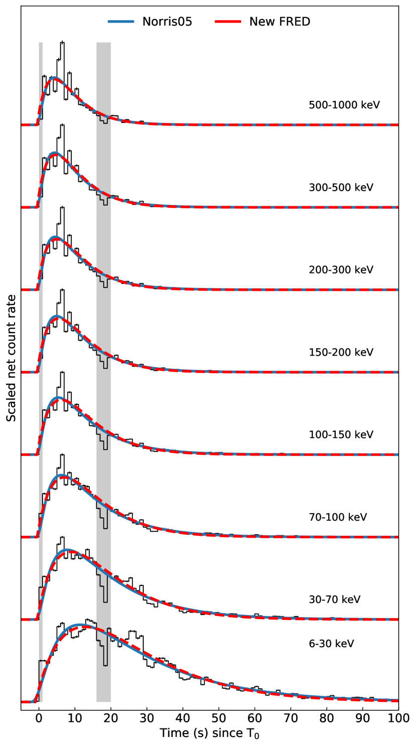
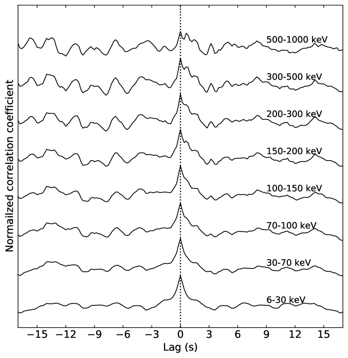
Figure 1: Temporal analysis of the GECAM multi-band light curves of GRB 230307A.
Left: The black histograms are binned net count rates (with background subtracted); The blue solid curves are best-fit FRED model with the Norris05 formulation, while the blue dashed curves are the best-fit with our new FRED formulation. Gray shadowed regions (the precursor and the dip) are ignored in the fitting. All error bars represent 1$\sigma$ uncertainties of the net count rates.
Upper right: The residuals of the net light curves after fitting with the new FRED formulation.
Lower right: The cross-correlation between the multi-band residuals and that in the 6-30 keV channel. The vertical dotted line indicates the zero lag time.

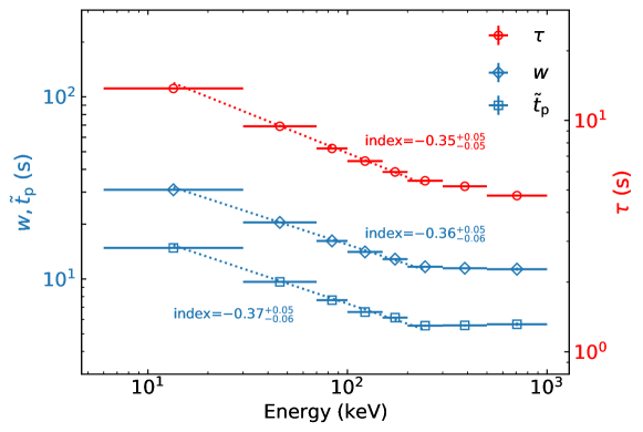
Figure 2: The fitted FRED formulation parameters as a function of energy. The vertical error bars indicate the 1$\sigma$ uncertainties of the fitted parameters, while the horizontal error bars indicate the ranges of the energy bins.

In order to further demonstrate the self-similar feature of the slow varying profile, we smooth the light curves in a non-parametrical way, and manifest their shape identity after energy-dependent re-scaling in time (see Methods). We stack all the re-scaled and smoothed light curves in the left panel of extended data Figure 1. It can be obviously shown that, the shape of the profiles in different energy bands can be "stretched" in time domain into an identical shape with an energy dependent scaling factor. The scaling factor as a function of energy is plotted in the right panel of extended data Figure 1.

The self-similarity inspired us to propose another formulation of FRED profile, with one less parameter than that of Norris05:

$$L(t)\propto\frac{t-t_{\rm{s}}}{\tau}\exp(-\frac{t-t_{\rm{s}}}{\tau}).$$ (2)

We fit the multi-band light curves again with the new FRED formulation. The results of fitting are listed in Methods. The sole time scale parameter $\tau$ shows a similar energy dependence on energy, $\tau\propto E^{-0.35^{+0.05}_{-0.05}}$, from 6 to 300 keV, and shows a hint of shallower energy dependence above $\sim 300$ keV (Figure 2). In the new formulation, one can define peak time as $t_{\rm p}=t_{s}+\tau_{E}$, where we denote the $\tau$ in the $E$ channel with $\tau_{E}$. The width of the FRED profile also scales as $\tau_{E}$. Therefore, the found $\tau-E$ dependence can naturally result in the $w-E$ and $\tilde{t}_{\rm{p}}-E$ relations.

Beside the self-similar FRED profile of the broad feature of GRB0307A’s light curve, the extraordinary brightness of the burst allows us to study the fast varying temporal structures. From the residuals of the light curves (upper right panel of Figure 1), one can see that there are many rapidly-varying short pulses. One noticeable feature is that even the broad pulse has a clear energy dependence, the short time spikes and dips appear to align at the same instances across different energy bands. We further demonstrate this alignment of the fast temporal features by cross-correlations among multi-band light curve residuals. As shown in the lower right panel of Figure 1, the peaks are perfectly aligned across the full energy band. This immediately excludes the attempt to explain the self-similar stretchable feature of the multi-band light curves as relativistic time-dilation, as a time-dilation effect would stretch both slow and fast varying pulses together.

We show that some of these prominent short duration structures can be fitted with individual short pulses (see Methods). The negative residuals, most prominently the dip at around $\sim$18 s in all energy bands, essentially excludes the possibility that short time structures are added onto a broad pulse component. It is also difficult to explain this dip as absorption, since the effective optical depth shows an energy dependence which no known absorption mechanism can reproduce (see Methods). The most likely explanation is that, the broad pulse of the light curves is composed of many fast pulses, and the dips are gaps between successive short pulses (see Methods).

The aforementioned results serve as important tests on the GRB prompt emission models. The internal shock models interpret short-time variabilities as a result of collisions of pairs of shells. As a result, the typical emission region is at[2, 4] $R_{\rm IS}\sim\Gamma^{2}c\delta t\simeq(3\times 10^{14}\ {\rm cm})(\Gamma/100)^{2}(\delta t/1\ {\rm s})$ from the central engine, where $\Gamma\sim 100$ is the bulk Lorentz factor of the GRB, and $\delta t\sim 1$ s is the typical variability time scale of the fast component. Within such a scenario, the broad pulse should be defined as the history of the central engine activity, which should be the same for all energy bands. The clear energy-dependence of the broad pulse abandons this interpretation and has to appeal to another internal shock at a much larger emission radius defined by $R_{2}\sim\Gamma^{2}c\Delta t\sim(1.2\times 10^{16}\ {\rm cm})(\Gamma/100)^{2}(\Delta t/40\ {\rm s})$ to interpret the slow component, where $\Delta t\sim 40$ s is the timescale of the broad pulse, which is essentially the GRB duration itself. Within such a picture, the observed emission should be the superposition between the fast and slow components, but the very deep, achromatic dip at around 18 s has essentially ruled out this possibility. We therefore conclude that the internal shock model is clearly disfavored.

The ICMART model, on the other hand, offers a natural interpretation to the data. Within this model[3, 5, 17], only the slow component with a characteristic timescale $\Delta t$ is related to the central engine activity duration and hence, the typical thickness of the magnetic blobs. The collision site between two magnetically-dominated shells is at $R_{\rm ICMART}=R_{2}\sim(1.2\times 10^{16}\ {\rm cm})(\Gamma/100)^{2}(\Delta t/40\ {\rm s})$. The rapid-varying fast component with timescale $\delta t$, on the other hand, is related to the emission timescale of local mini-jets within the global emission zone. The broad pulse is simply the superposition of emission of many mini-jets. No underlying slow component is needed. Significant dips are allowed, especially during the decay phase when high-latitude emission starts to play a role. The location of the dip is consistent with such a phase[11]. Because the fast pulses originate from local mini-jet events, the broad-band emission of the fast component is related to the dynamics of the mini-jets and therefore perfectly aligned in time.

The general trend of energy-dependent peak time and duration is naturally expected within the framework of the ICMART model. Unlike the internal shock model that attributes different short pulses as emission from different emitting fluids, the ICMART model suggests that the emission of the entire broad pulse originates from the same fluid as it expands in space. The magnetic field strength in the emission region decays with radius due to expansion[25], leading to rolling down of the characteristic synchrotron emission frequency with time. As result, higher energy emission peaks earlier and lasts shorter than lower energy emission[7, 26]. The general trend of model prediction matches the observations well[7], even though the self-similarity revealed from the data may require special model parameters, which may be related to the details of magnetic turbulence and reconnection in the emission region, and thus provide new insights into the physics of gamma-ray bursts.

1 Method

1.1 Observations

GECAM is a dedicated all-sky gamma-ray monitor constellation funded by the Chinese Academy of Sciences, and now consists of three telescopes, i.e. GECAM-A and GECAM-B[27] micro-satellties launched together on December 10, 2020, and GECAM-C (also called High Energy Burst Searcher, HEBS)[28] onboard SATech-01 experimental satellite launched on July 27, 2022. There are two kinds of detectors in each GECAM telescope: Gamma-Ray Detectors (GRDs) and Charged Particle Detectors (CPDs). GRDs are the main detector of GECAM, each of which is composed of a scintillator and an array of SiPMs. There are 25 GRDs onboard each of GECAM-A and GECAM-B, and 12 GRDs onboard GECAM-C.

GRB 230307A triggered GECAM-B in real-time at 15:44:06.650 UT on 7 March 2023 (denoted as T₀) and also detected by GECAM-C and other gamma-ray monitors (e.g. Fermi/GBM, Konus-Wind), while GECAM-A was offline at that time. The real-time alert data was transmitted instantly with the Global Short Message Communication of Beidou satellite navigation system[29, 30], and processed by the automatic pipeline of GECAM[31], based on which the extreme brightness of GRB 230307A was firstly reported by GECAM to the community[9], initiating many multi-wavelength follow-up observations[32, 33].

Thanks to the dedicated design of instrument[28, 34], neither GECAM-B nor GECAM-C suffered from data saturation during the whole burst of GRB 230307A despite of its extreme brightness[11]. High quality of GECAM data allow us to accurately measure the temporal and spectral properties of GRB 230307A. GRD04 of GECAM-B and GRD01 of GECAM-C are selected for the analysis of light curves because of their smallest incident angle to the direction of GRB 230307A. These two detectors both operate in two readout channels: high gain (HG) and low gain (LG), which are independent in terms of data processing, transmission, and dead-time.

At the time of this burst, GECAM-C GRDs have a lower energy detection threshold of about 6 keV (owing to less radiation damage on SiPM) while GECAM-B GRDs have a relatively higher energy detection threshold of about 30 keV. For GRD04 of GECAM-B, the energy range of HG channel data are used from about 30 keV to 300 keV while the energy range of LG channel data are used from about 300 keV to 1000 keV. For GRD01 of GECAM-C, only HG channel data are used with the energy range from 6 keV to 30 keV. Though the response of GRD01 of GECAM-C for 6-15 keV and GRD04 of GECAM-B for 300-700 keV is affected by the electronics, this does not have any effect on the analysis of light curves.

The background of GECAM-B is estimated by fitting the data from $T_{0}$-50 s to $T_{0}$-5 s and $T_{0}$+160 s to $T_{0}$+200 s with the first order polynomials. The background of GECAM-C is estimated by fitting the data from from $T_{0}$-20 s to $T_{0}$-1 s and $T_{0}$+170 s to $T_{0}$+600 s with a combination of the first and second-order exponential polynomials[11].

1.2 Time-binned light curve and broad pulse fitting

We divide the data into eight energy bands (1st to 8th channels), namely 6-30 keV, where the data are from GECAM-C; 30-70 keV, 70-100 keV, 100-150 keV, 150-200 keV, 200-300 keV, 300-500 keV and 500-1000 keV, where the data are from GECAM-B. The counts are binned every one second, and the background is subtracted to calculate the net count rate. The multiband net count rates are then fitted to both FRED formulation with Norris05 and our new FRED function (equations 1,2). The fittings are done with the maximum likelihood method, which can be expressed as ${\rm ln}\mathcal{L}=\sum_{i}\frac{({\rm DATA}_{i}-{\rm MODEL}_{i})^{2}}{\sigma_{i}^{2}}$ by assuming a Gaussian distribution of the observed net count rate, where the subscript i runs over all time bins from -4 s to 100 s (excluding 0 s to 1 s and 16 s to 20 s). The posteriors of the fitted parameters are found with a Monte Carlo Markov Chain (MCMC) method. The fitted parameters are listed in extended data Table 1.

In the upper-right panel of Figure 1, we plot the the FRED parameters, namely $w$ and $\tilde{t}_{\rm{p}}$ of Norris05 profile and $\tau$ of the new FRED profile, as functions of energy. The vertical error bars are the uncertainties of the fitted parameters, and the horizontal error bars indicate the width of each band. We fit power law relations between the FRED parameters and their corresponding energies. The power law fitting include the points from the 1st to the 6th channels (6-300 keV). The power index are -0.36${}^{+0.05}_{-0.06}$, -0.37${}^{+0.05}_{-0.06}$ and -0.35${}^{+0.05}_{-0.05}$ for $w-E$, $\tilde{t}_{\rm{p}}-E$ and $\tau-E$ relations respectively. The uncertainties of the power index are found with Monte-Carlo samplings of the FRED parameters and $E$ from their distributions. The distributions of the FRED parameters are assumed to be Gaussian with their fitted uncertainties, while the distribution of the energy is the corresponding energy deposition spectrum in each band.

Table 1: Fitting results for the net light curves of GRB 230307A. All errors represent the 1$\sigma$ uncertainties.

	Norris05				New FRED
Energy range	$\tau_{\rm r}$	$\tau_{\rm d}$	norm	ts	$\tau$	norm	ts
(keV)	(s)	(s)	(counts$\cdot$s-1)	(s)	(s)	(counts$\cdot$s-1)	(s)
6-30	$11.11^{+0.26}_{-0.26}$	$19.76^{+0.11}_{-0.10}$	$2.49^{+0.05}_{-0.05}\times 10^{4}$	$-3.42^{+0.09}_{-0.09}$	$13.74^{+0.03}_{-0.03}$	$1.47^{+0.004}_{-0.004}\times 10^{4}$	$-9.78^{+0.28}_{-0.29}\times 10^{-1}$
30-70	$6.84^{+0.13}_{-0.13}$	$13.61^{+0.06}_{-0.07}$	$2.08^{+0.04}_{-0.03}\times 10^{4}$	$-1.79^{+0.04}_{-0.04}$	$9.43^{+0.02}_{-0.02}$	$1.33^{+0.004}_{-0.004}\times 10^{4}$	$-5.16^{+0.08}_{-0.08}\times 10^{-1}$
70-100	$5.46^{+0.13}_{-0.12}$	$10.73^{+0.06}_{-0.06}$	$1.28^{+0.03}_{-0.03}\times 10^{4}$	$-1.39^{+0.04}_{-0.04}$	$7.56^{+0.02}_{-0.02}$	$8.05^{+0.03}_{-0.03}\times 10^{3}$	$-5.06^{+0.06}_{-0.05}\times 10^{-1}$
100-150	$4.55^{+0.10}_{-0.10}$	$9.52^{+0.05}_{-0.05}$	$1.52^{+0.03}_{-0.03}\times 10^{4}$	$-1.23^{+0.03}_{-0.03}$	$6.67^{+0.02}_{-0.02}$	$9.92^{+0.03}_{-0.04}\times 10^{3}$	$-5.08^{+0.04}_{-0.04}\times 10^{-1}$
150-200	$4.51^{+0.13}_{-0.12}$	$8.34^{+0.06}_{-0.06}$	$1.10^{+0.03}_{-0.03}\times 10^{4}$	$-1.25^{+0.04}_{-0.03}$	$5.98^{+0.02}_{-0.02}$	$6.60^{+0.03}_{-0.03}\times 10^{3}$	$-5.15^{+0.04}_{-0.05}\times 10^{-1}$
200-300	$3.99^{+0.13}_{-0.12}$	$7.68^{+0.06}_{-0.06}$	$9.96^{+0.28}_{-0.26}\times 10^{3}$	$-1.07^{+0.04}_{-0.04}$	$5.48^{+0.02}_{-0.02}$	$6.12^{+0.03}_{-0.03}\times 10^{3}$	$-4.98^{+0.07}_{-0.03}\times 10^{-1}$
300-500	$4.37^{+0.14}_{-0.15}$	$7.08^{+0.06}_{-0.06}$	$1.17^{+0.04}_{-0.04}\times 10^{4}$	$-1.23^{+0.04}_{-0.04}$	$5.19^{+0.02}_{-0.02}$	$6.35^{+0.03}_{-0.03}\times 10^{3}$	$-5.12^{+0.05}_{-0.05}\times 10^{-1}$
500-1000	$5.23^{+0.29}_{-0.28}$	$6.08^{+0.09}_{-0.09}$	$6.66^{+0.44}_{-0.40}\times 10^{3}$	$-1.38^{+0.07}_{-0.07}$	$4.73^{+0.03}_{-0.03}$	$2.74^{+0.02}_{-0.02}\times 10^{3}$	$-4.93^{+0.29}_{-0.15}\times 10^{-1}$

1.3 Profile self-similarity checking

In the left panel of extended data Figure 1, we stack the time re-scaled smoothed light curves, to show that the broad features of the light curves in different energy bands share the identical shapes. The smoothed light curves are convolution between a Gaussian kernel and the original light curves. The sigma of the Gaussian kernel is 1.5 s. We use the smoothed light curve in the 500-1000 keV band as the template, and we fit the template to light curves in other bands, which are scaled by multiplying scaling factors $\alpha_{\rm{E}}$ to the their time argument $T-T_{0}$. It is intuitively shown that the self-similarity of the broad profile, and this conclusion is FRED formulation independent. The scaling factor as a function of energy is plotted in the right panel of extended data Figure 1, which again shows a power law dependence.

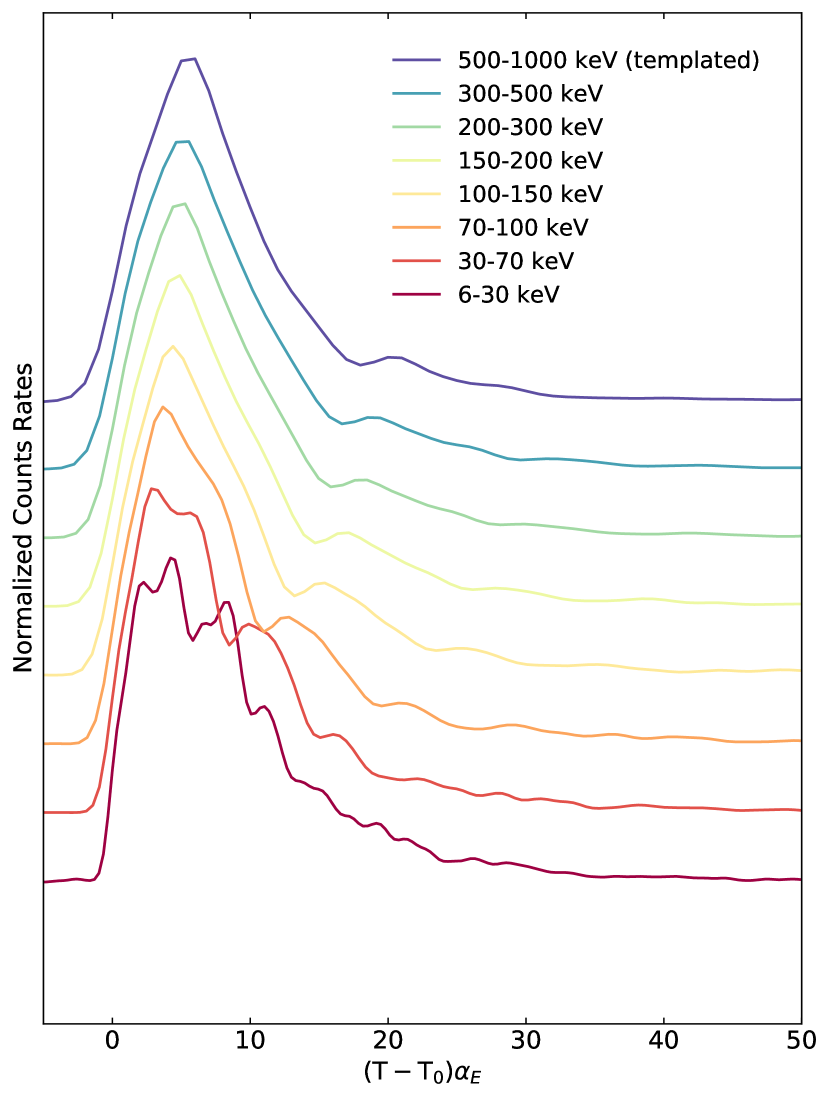
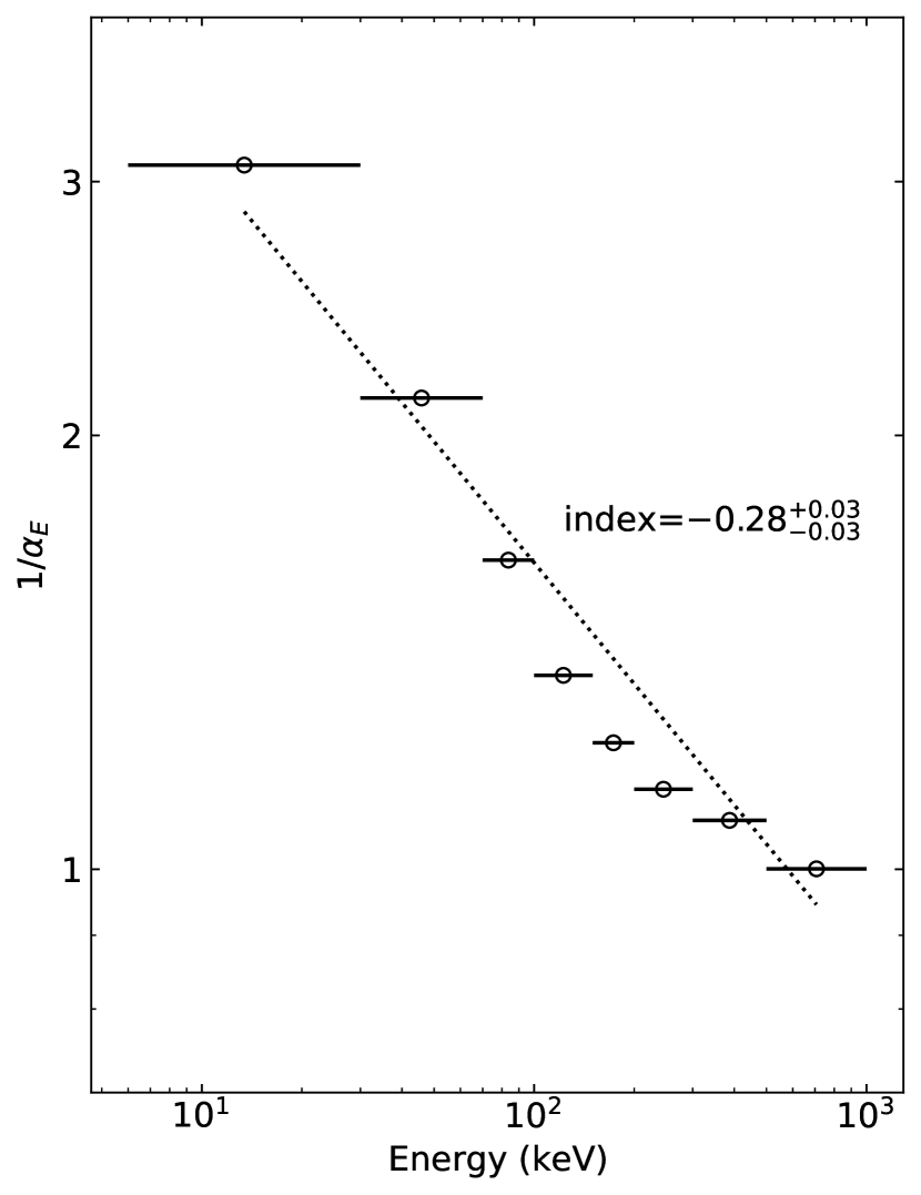
Figure 1: Left: The smoothed and time-rescaled GECAM multiband light curves of GRB 230307A.
Right: The scaling factor of the Gaussian smoothed light curve as a function of energy. The vertical error bars indicate the 1$\sigma$ uncertainties of the fitted parameters, while the horizontal error bars indicate the ranges of the energy bins.

1.4 Fast pulses

After the FRED profiles are removed from the multi-band light curves, the residuals show fast pulses (Upper right panel of Figure 1). It is shown clearly that the fast temporal structures are aligned in time across all energy ranges. Here, we further test this temporal alignment with cross-correlation between the residuals. In the lower right panel of Figure 1, we plot the normalized correlation coefficient as a function of lag time between the residuals in a certain band and that in band 6-30 keV. As we can see, all the cross-correlation peak at lag time zero, indicating the alignment of the fast pulses.

Here we further demonstrate that some of the prominent fast structures can be identified as small pulses. For instance, we show that the spike at $\sim 3.5$ s can be fitted with a pulse profile. We employ our new FRED formulation to fit the pulse from 3 s to 3.75 s, and find the typical width-$E$ relation ($\tau-E$ in the new FRED formulation) in GRB pulses. In order to show this conclusion is independent on the pulse profile formulation, we use Gaussian function as an alternative profile to fit the spike, and obtain the same width-$E$ relation ($\sigma-E$ with the Gaussian pulse formulation. See the lower right panel of extended data Figure 2). It can be seen in the left panel of extended data Figure 2 that the FRED profile results in a better fit than the Gaussian profile. The fitted parameters are list in extended data Table 2. It is also interesting to observe that this small pulse does not show spectrum lag of its peak time as the broad pulse. We demonstrate this by cross-correlating between the small pulses in multi-bands and that in 30-70 keV channel. The lag time together with their uncertainties as a function of energy is shown in the upper right panel of extended data Figure 2, where all lag times are almost zero, and we can clearly conclude that the lag time does not depend on energy like the broad pulse.

Table 2: Light curves fitting results for the fast varying temporal structure of light curves at about 3.5 s . All errors represent the 1$\sigma$ uncertainties.

	Gaussian			New FRED
Energy range	$\mu$	$\sigma$	norm	$\tau$	norm	ts
(keV)	(s)	(s)	(counts$\cdot$s-1)	(s)	(counts$\cdot$s-1)	(s)
30-70	$3.36^{+0.01}_{-0.01}$	$3.20^{+0.11}_{-0.09}\times 10^{-1}$	$4.78^{+0.09}_{-0.09}\times 10^{3}$	$2.88^{+0.09}_{-0.08}\times 10^{-1}$	$1.37^{+0.03}_{-0.03}\times 10^{4}$	$2.99^{+0.01}_{-0.01}$
70-100	$3.38^{+0.01}_{-0.01}$	$2.54^{+0.07}_{-0.07}\times 10^{-1}$	$3.64^{+0.08}_{-0.08}\times 10^{3}$	$2.54^{+0.07}_{-0.06}\times 10^{-1}$	$1.02^{+0.02}_{-0.02}\times 10^{4}$	$3.02^{+0.003}_{-0.003}$
100-150	$3.39^{+0.004}_{-0.004}$	$2.49^{+0.06}_{-0.05}\times 10^{-1}$	$5.09^{+0.09}_{-0.09}\times 10^{3}$	$2.28^{+0.07}_{-0.07}\times 10^{-1}$	$1.47^{+0.03}_{-0.03}\times 10^{4}$	$3.07^{+0.01}_{-0.01}$
150-200	$3.40^{+0.004}_{-0.004}$	$2.03^{+0.04}_{-0.03}\times 10^{-1}$	$4.08^{+0.09}_{-0.09}\times 10^{3}$	$1.93^{+0.05}_{-0.05}\times 10^{-1}$	$1.15^{+0.03}_{-0.03}\times 10^{4}$	$3.11^{+0.003}_{-0.004}$
200-300	$3.38^{+0.004}_{-0.004}$	$1.90^{+0.04}_{-0.03}\times 10^{-1}$	$4.24^{+0.09}_{-0.10}\times 10^{3}$	$1.76^{+0.04}_{-0.04}\times 10^{-1}$	$1.23^{+0.03}_{-0.03}\times 10^{4}$	$3.11^{+0.003}_{-0.004}$
300-500	$3.39^{+0.003}_{-0.004}$	$1.87^{+0.03}_{-0.03}\times 10^{-1}$	$4.46^{+0.09}_{-0.09}\times 10^{3}$	$1.73^{+0.04}_{-0.04}\times 10^{-1}$	$1.30^{+0.03}_{-0.03}\times 10^{4}$	$3.12^{+0.003}_{-0.003}$
500-1000	$3.37^{+0.004}_{-0.004}$	$1.46^{+0.03}_{-0.03}\times 10^{-1}$	$2.42^{+0.08}_{-0.08}\times 10^{3}$	$1.42^{+0.04}_{-0.04}\times 10^{-1}$	$6.72^{+0.22}_{-0.21}\times 10^{3}$	$3.13^{+0.003}_{-0.003}$

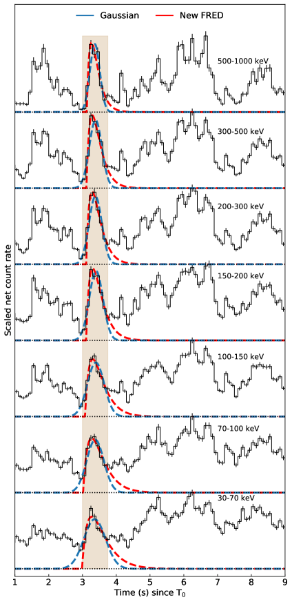
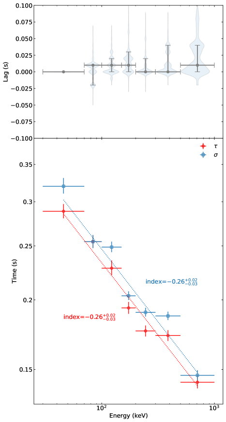
Figure 2: Left: Pulse profile fitting to the fast varying temporal structure at $\sim 3.5$ s. Red and blue dashed lines correspond to new FRED formulation and Gaussian profile respectively. The shadowed region indicates the range of data involved in the fitting. Upper right: Cross-correlation between the light curves of small pulse in multi-bands as functions of the energy. Lower right: The fitted width ($\tau$ for new FRED and $\sigma$ for Gaussian profile) of pulse at $\sim 3.5$ s as function of energy.

The dip at $\sim 18$ s is another noticeable feature of the multi-band light curves. A natural attempt is to attribute such a dip to some sort of absorption or geometrical blocking. We define the effective “optical depth" $\tau_{\rm{op},E}$ in different energy bands as:

$$\exp(-\tau_{\rm{op},E})=\frac{C_{\rm{dip},E}}{C_{\rm{slow},E}},$$ (3)

where $C_{\rm dip}$ is the net count rate at the bottom of the dip, which is found with a negative Gaussian fitting superposed on the FRED of broad pulse fitting from 17 s to 19.5 s (upper left panel of Extended Data Figure 3); and $C_{\rm slow}$ is the net count rate of the broad feature. The results of the fitting with a negative Gaussian is tabulate in extended data Table 3. It is intriguing to find that there is a power law energy dependence of the effective optical depth, and the best fit power law index is $\sim 0.4$ (the lower left panel of extended data Figure 3). This energy dependence of the optical depth challenges the absorption picture, for there is no known absorption mechanism whose cross section proportional to energy to the order of $\sim 0.4$.

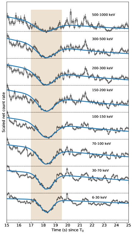
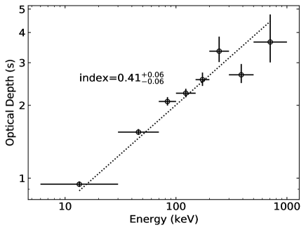
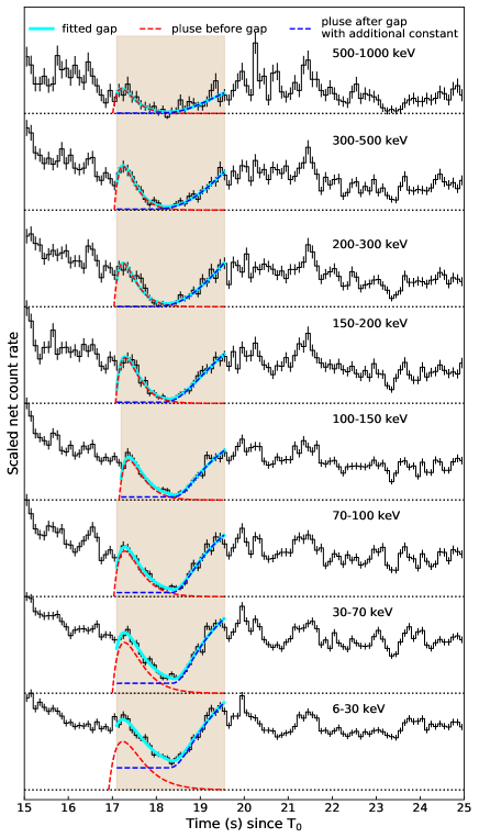
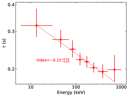
Figure 3: Upper left: fitting the gap with a FRED profile and a negative Gaussian function. The shadowed region indicates the range of data involved in the fitting. Lower left: the effective optical depth defined with equation 3, as a function of energy. Upper right: fitting the gap with two successive short pulses. The dashed red curves indicate the earlier pulse component, and the dashed blue curves indicate the rising edge of the later pulse. Cyan curves indicating the summation of these two components. Lower right: the time scale factor $\tau$ for new FRED of the earlier pulse component in the 18-s dip, as a function of energy.

Here we view the dip as gaps between two successive fast temporal structures. Therefore, we fit a pulse profile (new FRED formulation) and a rising edge of another pulse (Norris05) to the dip at each energy bands from $\sim$17 s to 19.5 s (the upper right panel of extended data Figure 3). The fitted parameters are list in extended data Table 4. The time scale $\tau$ of the earlier pulses as a function of energy is plotted in the lower right panel of extended data Figure 3, which shows clearly a typical power law energy dependence of pulse width.

Table 3: Light curves fitting results for the dip and optical depth. All errors represent the 1$\sigma$ uncertainties.

Energy range	$\mu$	$\sigma$	$C_{{\rm slow},E}$	Optical Depth
(keV)	(s)	(s)	(counts$\cdot$s-1)
6-30	$18.27^{+0.01}_{-0.01}$	$4.68^{+0.10}_{-0.09}\times 10^{-1}$	$5.08^{+0.01}_{-0.01}\times 10^{3}$	$0.94^{+0.03}_{-0.02}$
30-70	$18.25^{+0.01}_{-0.01}$	$5.51^{+0.10}_{-0.10}\times 10^{-1}$	$3.62^{+0.01}_{-0.01}\times 10^{3}$	$1.55^{+0.04}_{-0.04}$
70-100	$18.21^{+0.01}_{-0.01}$	$6.13^{+0.14}_{-0.13}\times 10^{-1}$	$1.68^{+0.01}_{-0.01}\times 10^{3}$	$2.07^{+0.09}_{-0.08}$
100-150	$18.25^{+0.01}_{-0.01}$	$6.99^{+0.15}_{-0.15}\times 10^{-1}$	$1.68^{+0.01}_{-0.01}\times 10^{3}$	$2.25^{+0.10}_{-0.09}$
150-200	$18.19^{+0.01}_{-0.01}$	$6.70^{+0.18}_{-0.18}\times 10^{-1}$	$9.06^{+0.05}_{-0.05}\times 10^{2}$	$2.55^{+0.18}_{-0.15}$
200-300	$18.19^{+0.01}_{-0.02}$	$6.77^{+0.21}_{-0.20}\times 10^{-1}$	$6.90^{+0.05}_{-0.05}\times 10^{2}$	$3.35^{+0.50}_{-0.33}$
300-500	$18.18^{+0.02}_{-0.02}$	$7.26^{+0.24}_{-0.23}\times 10^{-1}$	$6.23^{+0.05}_{-0.05}\times 10^{2}$	$2.67^{+0.29}_{-0.20}$
500-1000	$18.12^{+0.04}_{-0.04}$	$8.08^{+0.54}_{-0.47}\times 10^{-1}$	$2.11^{+0.03}_{-0.03}\times 10^{2}$	$3.65^{+1.10}_{-0.64}$

Table 4: Light curves fitting results for the gap with two successive fast temporal structures. All errors represent the 1$\sigma$ uncertainties.

	pluse before gap			pluse after gap			additional constant
Energy range	ts	$\tau$	norm	ts	$\tau_{\rm r}$	norm	constant
(keV)	(s)	(s)	(counts$\cdot$s-1)	(s)	(s)	(counts$\cdot$s-1)	(counts$\cdot$s-1)
6-30	$16.92^{+0.06}_{-0.10}$	$3.19^{+0.63}_{-0.37}\times 10^{-1}$	$9.22^{+0.87}_{-0.49}\times 10^{3}$	$18.13^{+0.07}_{-0.08}$	$1.29^{+0.25}_{-0.18}$	$1.13^{+0.19}_{-0.13}\times 10^{4}$	$1.54^{+0.20}_{-0.35}\times 10^{3}$
30-70	$17.00^{+0.03}_{-0.04}$	$2.74^{+0.30}_{-0.22}\times 10^{-1}$	$7.24^{+0.32}_{-0.28}\times 10^{3}$	$18.23^{+0.04}_{-0.07}$	$1.10^{+0.19}_{-0.08}$	$7.81^{+1.02}_{-0.47}\times 10^{3}$	$5.20^{+1.05}_{-1.48}\times 10^{2}$
70-100	$17.03^{+0.02}_{-0.03}$	$2.48^{+0.24}_{-0.21}\times 10^{-1}$	$3.42^{+0.15}_{-0.14}\times 10^{3}$	$18.21^{+0.05}_{-0.10}$	$1.16^{+0.31}_{-0.12}$	$3.76^{+0.74}_{-0.32}\times 10^{3}$	$1.11^{+0.46}_{-0.55}\times 10^{2}$
100-150	$17.15^{+0.02}_{-0.02}$	$2.21^{+0.17}_{-0.14}\times 10^{-1}$	$3.15^{+0.14}_{-0.13}\times 10^{3}$	$18.23^{+0.05}_{-0.07}$	$1.23^{+0.27}_{-0.16}$	$3.44^{+0.67}_{-0.37}\times 10^{3}$	$86.96^{+14.91}_{-27.78}$
150-200	$17.07^{+0.01}_{-0.02}$	$2.16^{+0.13}_{-0.13}\times 10^{-1}$	$1.97^{+0.10}_{-0.10}\times 10^{3}$	$17.89^{+0.18}_{-0.26}$	$2.25^{+1.28}_{-0.71}$	$2.98^{+2.08}_{-0.90}\times 10^{3}$	$17.23^{+19.08}_{-12.19}$
200-300	$17.04^{+0.02}_{-0.03}$	$2.03^{+0.12}_{-0.10}\times 10^{-1}$	$1.63^{+0.08}_{-0.09}\times 10^{3}$	$17.42^{+0.24}_{-0.21}$	$5.09^{+1.71}_{-1.55}$	$6.52^{+5.00}_{-2.79}\times 10^{3}$	$3.32^{+3.69}_{-2.44}$
300-500	$17.05^{+0.02}_{-0.04}$	$1.95^{+0.16}_{-0.13}\times 10^{-1}$	$1.59^{+0.10}_{-0.09}\times 10^{3}$	$17.30^{+0.25}_{-0.15}$	$5.86^{+1.23}_{-1.67}$	$6.76^{+3.92}_{-2.92}\times 10^{3}$	$11.75^{+7.42}_{-7.67}$
500-1000	$17.01^{+0.06}_{-0.18}$	$1.99^{+0.34}_{-0.24}\times 10^{-1}$	$4.43^{+0.76}_{-0.55}\times 10^{2}$	$17.66^{+0.32}_{-0.38}$	$3.69^{+2.80}_{-1.90}$	$9.28^{+16.28}_{-5.48}\times 10^{2}$	$1.91^{+2.61}_{-1.42}$

Data Availability

The processed data are presented in the tables and figures of the paper, which are available upon reasonable request.

Code Availability

Upon reasonable requests, the code (mostly in Python) used to produce the results and figures will be provided.

S.-X.Y. thanks the insightful discussion with Prof. Kinwah Wu on the origin of the self-similarity of the multi-wavelength lightcurves of the burst. S.-X.Y. also discussed with Dr. X.L. Wang on the potential physical implication of these interesting behaviour in data. This work is supported by the National Key R&D Program of China (2021YFA0718500). S.-X.Y. acknowledges support from the Chinese Academy of Sciences (grant Nos. E329A3M1 and E3545KU2). S.-L.X. acknowledges the support by the National Natural Science Foundation of China (Grant No. 12273042). The GECAM (Huairou-1) mission is supported by the Strategic Priority Research Program on Space Science (Grant No. XDA15360000) of Chinese Academy of Sciences. ChatGPT3.5 was used to check and correct a few sentences regarding their English grammar and wording, without any changes on their original meanings.

S.-L.X. and S.-X.Y. initiated the study. S.-X.Y. led the investigation and wrote the manuscript. B.Z. and S.-X.Y. proposed the physical implications of the data. S.-L.X. led the GECAM observation and data analysis. B.Z., C.-W.W., S.-L.X. contributed to the writing of the manuscript. C.-W.W. is the major contributor of GECAM data analysis. W.-J.T. investigated the nature of the dip $\sim 18$ s. S.-N.Z., R.M., S.-L.X. contributed to the theoretical interpretation of self-similarity of the broad pulse. W.-C.X. and J.-C.L. performed background analysis for GECAM-C. C.Z. and Y.-Q.Z. performed calibration analysis for GECAM. J.-C.L. performed the data saturation assessment for GECAM. P.Z. developed the data analysis tools for GECAM. Y.W. contributed to preparing of the manuscript. All authors participated in the discussion and proofreading of the manuscript, or contributed to the development and operation of GECAM, which is important for this work.

The authors declare that they have no competing financial interests.

Correspondence and requests for materials should be addressed to S.-X.Y.
(sxyi@ihep.ac.cn), C.-W.W. (cwwang@ihep.ac.cn), B.Z.(bing.zhang@unlv.edu), S.-L.X. (xiongsl@ihep.ac.cn).

References

- [1] Zhang, B. The Physics of Gamma-Ray Bursts (2018).
- [2] Rees, M. J. & Meszaros, P. Unsteady Outflow Models for Cosmological Gamma-Ray Bursts. ApJ 430, L93 (1994). astro-ph/9404038.
- [3] Zhang, B. & Yan, H. The Internal-collision-induced Magnetic Reconnection and Turbulence (ICMART) Model of Gamma-ray Bursts. ApJ 726, 90 (2011). 1011.1197.
- [4] Kobayashi, S., Piran, T. & Sari, R. Can Internal Shocks Produce the Variability in Gamma-Ray Bursts? ApJ 490, 92 (1997). astro-ph/9705013.
- [5] Zhang, B. & Zhang, B. Gamma-Ray Burst Prompt Emission Light Curves and Power Density Spectra in the ICMART Model. ApJ 782, 92 (2014). 1312.7701.
- [6] Daigne, F. & Mochkovitch, R. Gamma-ray bursts from internal shocks in a relativistic wind: temporal and spectral properties. MNRAS 296, 275–286 (1998). astro-ph/9801245.
- [7] Uhm, Z. L. & Zhang, B. Toward an Understanding of GRB Prompt Emission Mechanism. I. The Origin of Spectral Lags. ApJ 825, 97 (2016). 1511.08807.
- [8] Fermi GBM Team. GRB 230307A: Fermi GBM Final Real-time Localization. GRB Coordinates Network 33405, 1 (2023).
- [9] Xiong, S., Wang, C., Huang, Y. & Gecam Team. GRB 230307A: GECAM detection of an extremely bright burst. GRB Coordinates Network 33406, 1 (2023).
- [10] Levan, A. et al. JWST detection of heavy neutron capture elements in a compact object merger. arXiv e-prints arXiv:2307.02098 (2023). 2307.02098.
- [11] Sun, H. et al. Magnetar emergence in a peculiar gamma-ray burst from a compact star merger. arXiv e-prints arXiv:2307.05689 (2023). 2307.05689.
- [12] Fenimore, E. E., in ’t Zand, J. J. M., Norris, J. P., Bonnell, J. T. & Nemiroff, R. J. Gamma-Ray Burst Peak Duration as a Function of Energy. ApJ 448, L101 (1995). astro-ph/9504075.
- [13] Shen, R.-F., Song, L.-M. & Li, Z. Spectral lags and the energy dependence of pulse width in gamma-ray bursts: contributions from the relativistic curvature effect. MNRAS 362, 59–65 (2005). astro-ph/0505276.
- [14] Liang, E.-W. et al. Temporal Profiles and Spectral Lags of XRF 060218. ApJ 653, L81–L84 (2006). astro-ph/0610956.
- [15] Kazanas, D., Titarchuk, L. G. & Hua, X.-M. The Duration–Photon Energy Relation of Gamma-Ray Bursts and Its Interpretations. ApJ 493, 708–714 (1998). astro-ph/9709180.
- [16] Qin, Y. P., Dong, Y. M., Lu, R. J., Zhang, B. B. & Jia, L. W. Relationship between the Gamma-Ray Burst Pulse Width and Energy Due to the Doppler Effect of Fireballs. ApJ 632, 1008–1020 (2005). astro-ph/0411365.
- [17] Shao, X. & Gao, H. Gamma-Ray Burst Prompt Emission Spectrum and E p Evolution Patterns in the ICMART Model. ApJ 927, 173 (2022). 2201.03750.
- [18] Lyutikov, M. & Blandford, R. Gamma Ray Bursts as Electromagnetic Outflows. arXiv e-prints astro–ph/0312347 (2003). astro-ph/0312347.
- [19] Narayan, R. & Kumar, P. A turbulent model of gamma-ray burst variability. MNRAS 394, L117–L120 (2009). 0812.0018.
- [20] Lazarian, A., Zhang, B. & Xu, S. Gamma-Ray Bursts Induced by Turbulent Reconnection. ApJ 882, 184 (2019). 1801.04061.
- [21] Hascoët, R., Daigne, F. & Mochkovitch, R. Accounting for the XRT early steep decay in models of the prompt gamma-ray burst emission. A&A 542, L29 (2012). 1206.6770.
- [22] Norris, J. P. et al. Long-Lag, Wide-Pulse Gamma-Ray Bursts. ApJ 627, 324–345 (2005). astro-ph/0503383.
- [23] Hakkila, J., Giblin, T. W., Norris, J. P., Fragile, P. C. & Bonnell, J. T. Correlations between Lag, Luminosity, and Duration in Gamma-Ray Burst Pulses. ApJ 677, L81 (2008). 0803.1655.
- [24] Peng, Z. Y., Zhao, X. H., Yin, Y., Bao, Y. Y. & Ma, L. Energy-dependent Gamma-Ray Burst Pulse Width Due to the Curvature Effect and Intrinsic Band Spectrum. ApJ 752, 132 (2012). 1204.3420.
- [25] Uhm, Z. L. & Zhang, B. Fast-cooling synchrotron radiation in a decaying magnetic field and -ray burst emission mechanism. Nature Physics 10, 351–356 (2014). 1303.2704.
- [26] Uhm, Z. L., Zhang, B. & Racusin, J. Toward an Understanding of GRB Prompt Emission Mechanism. II. Patterns of Peak Energy Evolution and Their Connection to Spectral Lags. ApJ 869, 100 (2018). 1801.09183.
- [27] Li, X. Q. et al. The technology for detection of gamma-ray burst with GECAM satellite. Radiation Detection Technology and Methods 6, 12–25 (2021).
- [28] Zhang, D. et al. The performance of SiPM-based gamma-ray detector (GRD) of GECAM-C. Nuclear Instruments and Methods in Physics Research A 1056, 168586 (2023). 2303.00537.
- [29] Zhao, X.-Y. et al. The In-Flight Realtime Trigger and Localization Software of GECAM. arXiv e-prints arXiv:2112.05101 (2021).
- [30] Guo, S. et al. Integrated Navigation and Communication Service for LEO Satellites Based on BDS-3 Global Short Message Communication. IEEE Access 11, 6623–6631 (2023).
- [31] Huang, Y. et al. The GECAM Real-Time Burst Alert System. arXiv e-prints arXiv:2307.04999 (2023).
- [32] Bom, C. R. et al. GRB 230307A: SOAR/Goodman detection of the possible host galaxy. GRB Coordinates Network 33459, 1 (2023).
- [33] Levan, A. J. et al. GRB 230307A: JWST observations consistent with the presence of a kilonova. GRB Coordinates Network 33569, 1 (2023).
- [34] Liu, Y. et al. The sipm array data acquisition algorithm applied to the gecam satellite payload. Radiation Detection Technology and Methods 6, 70–77 (2021).