GAMMA RAY BURSTS AS ELECTROMAGNETIC OUTFLOWS

Abstract

We interpret gamma ray bursts as relativistic, electromagnetic explosions. Specifically, we propose that they are created when a rotating, relativistic, stellar-mass progenitor loses much of its rotational energy in the form of a Poynting flux during an active period lasting $\sim 100$ s. Initially, a non-spherically symmetric, electromagnetically-dominated bubble expands non-relativistically inside the star, most rapidly along the rotational axis of the progenitor. After the bubble breaks out from the stellar surface and most of the electron-positron pairs annihilate, the bubble expansion becomes highly relativistic. After the end of the source activity most of the electromagnetic energy is concentrated in a thin shell inside the contact discontinuity between the ejecta and the shocked circumstellar material. This electromagnetic shell pushes a relativistic blast wave into the circumstellar medium. Current-driven instabilities develop in this shell at a radius $\sim 3\times 10^{16}$ cm and lead to dissipation of magnetic field and acceleration of pairs which are responsible for the $\gamma$-ray burst. At larger radii, the energy contained in the electromagnetic shell is mostly transferred to the preceding blast wave. Particles accelerated at the forward shock may combine with electromagnetic field from the electromagnetic shell to produce the afterglow emission.

In this paper, we concentrate on the dynamics of electromagnetic explosions. We describe the principles that control how energy is released by the central compact object and interpret the expanding electromagnetic bubble as an electrical circuit. We analyze the electrodynamical properties of the bubble and the shell, paying special attention to the energetics and causal behavior. We discuss the implication of the model for the afterglow dynamics and briefly discuss observational ramifications of this model of $\gamma$-ray bursts.

1 Introduction

In recent years, a “fireball/internal shock” model of “long” gamma-ray bursts (henceforth GRBs) has been developed (e.g.  Mészáros, 2002; Piran, 1999, and references therein). This associates GRBs with black hole or neutron star formation during the explosion of rapidly rotating, evolved, massive stars - the “collapsar” model. It is proposed that ultra-relativistic jets are formed within the spinning star and that these jets are subsequently responsible for the $\gamma$-ray emission and the afterglow Woosley et al.  (2003). This model has been supported by the discovery that GRBs occur preferentially in star-forming regions in cosmologically distant galaxies (e.g.  Bloom, Kulkarni & Djorgovski, 2001), that achromatic breaks (e.g.  Harrison et al. , 2001), indicative of beaming, have been observed in some afterglows and the observation of additional luminous components to the late afterglow (e.g.  Bloom et al. , 2002), which have recently been shown to have a supernova spectrum (e.g.  Hjorth et al. , 2003) in the case of SN 2003dh – GRB 030329. The principal phases in this model comprise:

I Energy Release

A source of power associated with a relativistic stellar mass object, now thought to be embedded within a star in the case of the long bursts, with luminosity $L=10^{50}L_{{\rm s,50}}$ erg s^-1 operates for a time $t_{{\rm s}}=100t_{{\rm s,2}}$ s within a region with radius $r_{{\rm s}}=10^{6}r_{{\rm s,6}}$ cm. The energy stored in a combined rotational, gravitational and internal form is at least $\sim 10^{52}L_{50}t_{{\rm s,2}}$ erg. The energy release mechanism may involve the release of magnetic energy by a torus (e.g.  Woosley, 1993; Vietri, 1998), a nascent magnetar with initial angular velocity $\sim 10^{4}$ rad s^-1 (e.g.  Usov, 1992; Duncan & Thompson, 1992; Thompson, 1994; Usov, 1994) or a black hole (e.g.  Paczyński, 1986). The magnetic field itself may be produced by strong dynamo activity (e.g.  Thompson & Murray, 2001) or shear (Kluzniak & Ruderman, 1998). Interpreting $r_{s}$ as the characteristic size of the light cylinder, the associated strength of the magnetic field is $B_{s}\sim 10^{14}L_{50}^{1/2}r_{s}^{-1}$ G. In an alternative class of models, the energy release involve the formation of a pair plasma by $\mathrel{\raise 1.29167pt\hbox{$>$}\mkern-14.0mu\lower 2.58334pt\hbox{$\sim$}}3$ MeV neutrinos (e.g.  Eichler et al. , 1989). Independent of the source, it is generally supposed that a high effective temperature $T_{{\rm s}}=T_{{\rm s,0}}{\rm MeV}\sim(L/4\pi r_{{\rm s}}^{2}\sigma_{SB})^{1/4}\sim L_{50}^{1/4}r_{{\rm s,6}}^{-1/2}$ MeV and entropy per baryon ($S=10^{6}S_{6}$ k), optically thick ($\tau_{T}\sim 10^{14}L_{50}^{3/4}r_{{\rm s,6}}^{-1}$) fireball is produced (Cavallo & Rees, 1978), varying on a timescale $t_{\rm var}\sim r_{{\rm s}}/c\sim 100r_{{\rm s,6}}\ \mu{\rm s}$. Long bursts are argued to have $L_{50}\sim t_{{\rm s,2}}\sim r_{{\rm s,6}}\sim S_{6}\sim 1$ (e.g.  Frail et al. , 2001).

II Flow Formation

As the radiation-dominated fireball expands due to “lepto-photonic” pressure, the flow is collimated by the surrounding stellar envelope into two anti-parallel jets with opening angle $\theta=0.1\theta_{-1}$. During the subsequent expansion, the energy is converted into ion bulk motion, and becomes matter-dominated at a radius, $r_{{\rm mat}}\sim 10^{10}$ cm, where the fluid Lorentz factor saturates with a value $\Gamma_{0}=10^{3}\Gamma_{{\rm 0,3}}\sim S(kT_{{\rm s}}/m_{p}c^{2})\sim 10^{3}$; beyond this radius, most of the energy resides in the kinetic energy of the protons. (The stellar photosphere is thought to have a similar radius.) The photons decouple from the plasma at a photospheric radius, $r_{{\rm phot}}$ which is also in the vicinity of $r_{{\rm mat}}$ for the envisaged conditions.

III $\gamma$-ray Burst

Much of the jet power is dissipated through a series of internal shocks at a radius $r_{\gamma}\sim\Gamma_{0}^{2}ct_{{\rm var}}\sim 3\times 10^{12}\Gamma_{0,3}^{2}$ cm. These shocks are responsible for the re-acceleration of relativistic electrons and the production of magnetic field and Doppler-shifted, $\gamma$-ray synchrotron emission, up to $\sim$ GeV energies, that is sufficiently well-collimated by the relativistic outflow to escape pair production. This is the Gamma-Ray Burst (GRB). The constraint that the highest energy $\gamma$-rays be able to escape without producing electron-positron pairs, implies that $\Gamma_{0,3}\sim 0.3$ (e.g.  Lithwick & Sari, 2001).

IV Afterglow

When $r>ct_{{\rm s}}/\theta\sim 10^{13}t_{{\rm s,-4}}\theta_{-1}^{-1}$, the debris takes the from of a shell of cold protons driving a blast wave into the surrounding medium with density $n=0.1n_{-1}{\rm cm}^{-3}$. An external shock forms and when $r\sim r_{{\rm rsh}}\sim 10^{16}L_{50}^{1/2}\theta_{-1}^{-1}\Gamma_{03}^{2}n_{-1}$ cm, a reverse shock will also form in the exploding debris. The debris decelerates after $r>r_{{\rm free}}\sim 6\times 10^{16}L_{50}^{1/2}t_{{\rm s,2}}^{1/2}n_{-1}^{-1/2}\theta_{-1}^{-1}\Gamma_{3}^{-1}$ cm The bipolar blast wave, formed by the shocked circumstellar medium, which now carries most of the energy of the explosion, will further decelerate according to $\Gamma\sim\Gamma_{0}(r/r_{{\rm free}})^{-3/2}$ until it becomes non-relativistic at a radius $r_{{\rm nr}}\sim\Gamma_{0}^{2/3}r_{{\rm free}}\sim 10^{18}$ cm. During this phase, electrons are accelerated and magnetic field is amplified at the outer shock, leading to the formation of the afterglow. The non-relativistic blast wave gradually becomes more spherical and evolves to resemble a normal, supernova remnant.

2 Some Problems with the Fireball Model

The basic fireball model, which we have just sketched, along with its many variations, raises several, important questions. Included among these, in temporal order of the flow evolution, are:

1. How is the entropy of the fireball created?

In most models, the release of energy is mediated by a strong electromagnetic field which is invoked to create turbulence in an accretion disk (e.g.  MacFadyen & Woosley, 1999), extract the rotational energy of the central black hole (e.g.  Kim et al. , 2002) and collimate and confine the jets (e.g.  MacFadyen & Woosley, 1999). As the energy release phase lasts for $\sim ct_{s}/r_{s}\sim 10^{6}$ source dynamical times, the magnetic flux must presumably be tied to or trapped by a large, conducting mass and the transients should die away so that a quasi-steady, electromagnetic energy flow will be produced, similar to what happens with pulsars. The problem is that, if the burst is powered electromagnetically, how is the large entropy of a fireball created? As we discuss further below, there is no natural way to accomplish this in the vicinity of the source, although there have been suggestions invoking magnetic reconnection in an outflowing wind. (Of course, this is not a concern for those models (e.g.  Salmonson et al. , 2001) where the energy release is mediated by neutrinos.)

2. How are the hypersonic jets made?

The fireball model requires that two jets are formed with Mach number $M\sim 2^{1/2}\Gamma_{0}\sim 400$ and a ratio of bulk kinetic energy to internal energy $\mathrel{\raise 1.29167pt\hbox{$>$}\mkern-14.0mu\lower 2.58334pt\hbox{$\sim$}}M^{2}\sim 10^{5}$. Numerical simulations (e.g.  Aloy et al. , 2002; MacFadyen et al. , 2003) and experience with wind tunnels strongly suggest that instability and entrainment prevent this from happening inside the star. It is more reasonable to suppose that the outflow emerges from the stellar surface (radius $R_{\ast}\equiv 10^{10}R_{\ast,10}$ cm) with a modest Lorentz factor $\Gamma_{\ast}$, collimated within a cone with opening angle $\theta\sim\Gamma_{\ast}^{-1}$. It will then accelerate linearly $\Gamma\propto r$ due to radiative pressure until either the momentum flux of the radiation field falls below that of the ions, or optical depth to Thomson scattering falls below unity. For ion jet the raping radius is (Eq. 22) $r(\tau=1)=3\times 10^{1}2{\rm cm}L_{50}\Gamma_{2.5}^{-3}\Delta\Omega_{-2}$. Thus, if an ion jet starts at $R_{\ast}\sim 10^{10}$ cm with $\Gamma_{\ast}\sim$ a few, it barely has enough optical depth to accelerate to the required $\Gamma\sim 300$. (Note that in this case most acceleration happens beyond the photosphere (for a ion jet) at $r_{ph}\sim 10^{11}$ cm, see Eq. (15).)

3. How can the outflow develop large, parallel, proper velocity gradients and avoid producing converging streams?

$O(1)$ gradients in the jet proper velocity are invoked in the fireball model in order to produce internal shocks, and supply the free energy for particle acceleration. The model is essentially one dimensional. It is usually supposed that this variation has its origin in the source which implies that the GRB be produced within a radius $\mathrel{\raise 1.29167pt\hbox{$>$}\mkern-14.0mu\lower 2.58334pt\hbox{$\sim$}}\Gamma^{2}ct_{{\rm min}}$ where $t_{{\rm min}}$ is the minimum variation timescale. However, it is also envisaged that the jet be collimated and develop $\sim(\Gamma\theta)^{2}$ causally disconnected streams. It is difficult to understand how this collimation can be achieved without producing angular deflections $\mathrel{\raise 1.29167pt\hbox{$>$}\mkern-14.0mu\lower 2.58334pt\hbox{$\sim$}}\Gamma^{-1}$ which would lead to pair formation by the escaping, high energy $\gamma$-rays. (This problem is analogous to the one addressed in contemporary cosmology by the theory of inflation with the important difference that, here, it must be solved in a continuous flow with a bounding surface.)

4. What determines the baryon loading of the flow?

Independent of the problem addressed in (2), in the fireball model, the baryon fraction must be fine-tuned to allow baryons to assume most of the energy of the outflow and to attain the large outflow Lorentz factors that are necessary; too small a fraction and the energy will escape before the baryon acceleration is complete, too large a fraction and the asymptotic Lorentz factor will be too low to allow the highest energy $\gamma$-rays to escape (e.g.  Mészáros, 2002).

5. Where are the thermal precursors?

For ion jets, the escape of thermal radiation at the photosphere should produce a thermal precursor with luminosity similar to the main burst (Lyutikov & Usov, 2000; Mészáros & Rees, 2000). These are rarely seen at the 1% level (Daigne & Mochkovitch, 2002; Frontera et al. , 2001; Ghirlanda et al. , 2003).

6. How are particles accelerated at relativistic shock fronts?

Diffusive shock acceleration, which appears to operate efficiently at non-relativistic shock fronts, fails at relativistic shocks, both in the $\gamma$-ray emitting region and at the external shock front, because only a minority of the back-scattered particles can catch up with the advancing shock front. There are promising, kinematic proposals (e.g.  Achterberg et al. , 2001) for addressing relativistic shock acceleration. However, they pre-suppose the existence of a subshock in the background thermal plasma and it is not clear how this can be maintained. (Actually, thermal and nonthermal particles are not really distinguished in emission models as it is generally assumed that a single, truncated, power-law distribution function is transmitted (e.g.  Blandford & McKee, 1977).) More fundamentally, it is by no means certain that relativistic shock discontinuities form at all. It may happen that the sharing of momentum between a relativistic outflow and the circumstellar medium happens gradually rather than abruptly (e.g.  Usov, 1994).

7. How is the magnetic field amplified?

In order to produce a high radiative efficiency and fit the afterglow light curves, it is necessary for the post-shock magnetic field strength be amplified by a large factor over the value it would have due to simple compression. It has been proposed that this amplification is due to the Weibel instability (e.g.  Medvedev & Loeb, 1999). Recent simulations have convincingly shown that a long coherence range (much larger than the ion skin depth) of the magnetic field field fluctuation is indeed reached Nishikawa et al.  (2003); Frederiksen et al.  (2003). However, the average values of the magnetic energy density, $\epsilon_{B}\sim 10^{-3}$ of the total energy density, is often too low to account for observed synchrotron emission.

8. How is a large degree of $\gamma$-ray polarization created?

A very high linear polarization (nominally 80 percent) has been reported in RHESSI observations of GRB021206 (Coburn & Boggs, 2003). The observation, if typical, is inconsistent with the internal shock model (Lyutikov, 2003b) In order to reproduce high polarization the internal shock model should make a number of high unlikely assumptions, some of which contradict the very fundamentals of the model. There are four assumptions that are made. (i) the field is confined to two dimensional plane, presumably the plane of the shock. Magnetic field amplification due to Weibel instability at the shock indeed produces two dimensional fields Medvedev & Loeb (1999); Nishikawa et al.  (2003); Frederiksen et al.  (2003), but the typical size of resulting magnetic structures with linearly directed currents is still microscopic, probably tens or hundreds of ion skin depths (which is of the order of meters when the fireball is $\sim 10^{12}$ cm in size). On larger scales, magnetic field is likely to be three dimensionally random. In addition, the postshock material must be turbulent: in the fireball model turbulence is needed in order to accelerate particle. In order to account for large energy fraction in accelerated electrons the turbulent motions should have energy density comparable to the total energy in the shock and thus much larger than the energy density in the magnetic field, typically $\epsilon_{B}\leq 10^{-3}$. This turbulence will easily destroy any finely-tuned current structures. (ii) the plane of the turbulent magnetic field is viewed edge-on in the rest frame (this requires viewing angle $\sim 1/\Gamma$ in the observer frame); (iii) the emitting surface should be quasi-planar; this requires that the angular size of the emitting region be $\Delta\theta\leq 1/\Gamma$. (iv) all emitting shells must have the same Lorentz factor to be seen edge on (the burst GRB030329 was multi-peaked). Assumptions (ii), (iii) and (iv) are at variance with the fundamental assumption of the internal shock/fireball model that every peak is interpreted as being due to collisions of shells with a range of Lorentz factors.

9. What determines the jet opening angle and its structure?

A number of phenomenological jet structures have been proposed (e.g. structured, constant or patchy jet). The fireball model neither gives a prediction or expresses a preference for the jet structure.

10. What is the relation between GRBs and X-ray flashes (XRFs)?

In the fireball model there is no clear relation between GRBs and XRFs, which can be either dirty fireballs, less energetic fireballs, or explosions seen ”from the side”.

11. Where are “orphan” afterglows?

If the GRB and afterglow emission is associated with jets, as described above, then in the most simplistic interpretation, there will be $\sim\theta^{-2}\sim 100\theta_{-1}^{-2}$ “orphan” afterglows expected per GRB. Although the current observational constraints are surprisingly poor and the expected number is quite model-dependent, it is surprising that no convincing examples have been found so far (e.g.  Levinson et al. , 2002).

3 Electromagnetic model

3.1 Overview

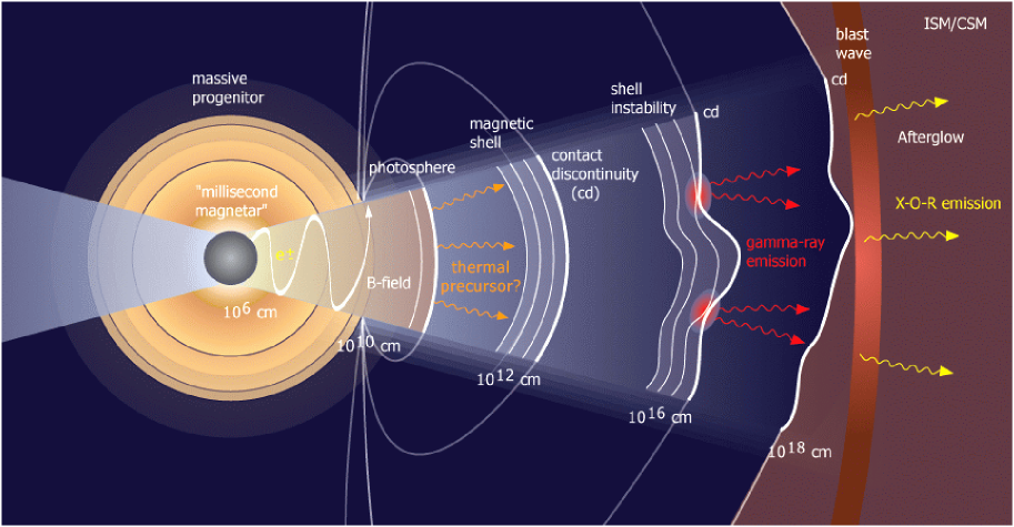
Figure 1: Overall view of the model.

In an attempt to retain the merits of the standard model while addressing these questions, we present an alternative, electromagnetic interpretation of GRBs that builds upon earlier models of electromagnetic and magnetohydrodynamic explosions (e.g.  Blandford & Rees, 1972; Benford, 1978; Usov, 1992, 1994; Mészáros & Rees, 1992; Ferrari, 1998; Kluzniak & Ruderman, 1998; Vietri, 1998; Spruit, 1999; Wheeler et al. , 2000; Lyutikov & Blackman, 2000; Vlahakis & Königl, 2001; Blandford, 2002; Lyutikov & Blandford, 2002). In our specific version of the electromagnetic model, we give a quite different interpretation of the same four phases of a GRB introduced in Section 1 (see also Fig. 1). At this point we do not have detail answers to all the posed questions; in some cases we offer only a plausible explanation. Also, we specialize to the collapsar model although the principles that we describe are easily adapted to other source models that may still be needed for the majority of GRBs.

I Source Formation (Energy Release)

The GRB “prime mover” is a rapidly spinning black hole orbited by a massive disk that has just been formed inside an imploding star, or, alternatively, a “millisecond magnetar”. For qualitative estimates we may use “millisecond magnetar” model by Usov (1992) (see also Blandford & Rees, 1972), though the numbers will be similar for any relativistic stellar mass source rotating with near-critical spin frequency $\sim 3L_{50}^{1/2}t_{s2}^{1/2}$ kHz and magnetic field of $B_{s}\sim 10^{14}L_{50}^{1/2}$ G. The total rotational energy, $E\sim I\Omega^{2}/2\sim Lt_{s}\sim 10^{52}$ erg is available to power GRB bursts and the magnetic field is strong enough for this energy to be released electromagnetically in a time $t_{s}\sim 10-100$ s.

We suppose that the outflow primarily takes the form of a large scale Poynting flux and that the dissipation rate remains low enough that the power continues to be dominated by the electromagnetic component rather than the heat of a fireball well out into the emission region, although there is almost certainly an initial phase in which the electromagnetic field is accompanied by a dense pair plasma.

A rapidly spinning magnetar with a complicated field structure will form a relativistic outflow. The behavior of such sources remains an unsolved problem, even in the simpler case of pulsar winds. In this paper we adopt a simplifying hypothesis, that the field lines quickly re-arrange to become predominantly axisymmetric. Thus we hypothesize that the axisymmetric or “DC” component of the electromagnetic field dominates the wave or “AC” component which is either dissipated as heat or diminished through non-dissipative rearrangement. In this case the electromagnetic source acts primarily as a unipolar inductor and drives a large quadrupolar current flow, rather like what happens in the Goldreich & Julian (1969) model of an axisymmetric pulsar.

II Bubble Inflation (Flow Formation)

Initially, the source will inflate an electromagnetic bubble inside the star. This magnetized cavity is separated from the outside material by the (tangential) contact discontinuity (CD) containing a surface Chapman-Ferraro current. This current terminates the magnetic field and completes the circuit that is driven by the source. On a microphysical level the current is created by the particle of the surrounding medium completing half a turn in the magnetic field of the bubble, so that the thickness of the current-currying layer is of the order of ion gyro-radius.

As we show below, the electromagnetic field can be treated as a fluid and behaves similarly to a true fluid, with the important difference that the rest frame stress tensor is anisotropic. This allows it to self-collimate (for reviews of stationary flow see, e.g.  Königl & Pudritz, 2000; Sauty et al. , 2002; Heyvaerts & Norman, 2003). The poloidal and toroidal components of magnetic field are comparable in strength at the light cylinder, but the toroidal field dominates beyond this. The velocity of expansion of the bubble is determined by the pressure balance on the contact discontinuity between magnetic pressure in the bubble and the ram pressure of the stellar material . As the magnetic field strength is strongest close to the symmetry axis, the bubble will expand fastest along the polar direction. Eventually the bubble will break free of its surroundings and forming a “twin exhaust” along which Poynting flux will flow until either the central source slows down or the collimating material itself expands which will both occur naturally on the timescale $t_{s}\sim 100$ s.

Outside the star, the bubble will expand ultrarelativistically and bi-conically. After it has expanded beyond a radius

$$r_{{\rm sh}}\sim ct_{s}\sim 3\times 10^{12}t_{s,2}{\rm cm}$$ (1)

the electromagnetic energy will be concentrated within an expanding, electromagnetic shell with thickness $\sim r_{{\rm sh}}$ and with most of the return current completing along its trailing surface. However, the global dynamics of this shell and its subsequent expansion are set in place by the electromagnetic conditions at the light cylinder and within the collimation region.

After break out, the interaction of the magnetic shell with the circumstellar medium proceeds in a similar way, except now the velocity of expansion is strongly relativistic. The leading surface of the shell is separated by a contact discontinuity (which actually becomes a rotational discontinuity if the circumstellar medium is magnetized (Lyutikov, 2002a)). Outside the CD an ultra-relativistic shock front may form and propagate into the surrounding circumstellar medium. The expansion will still be non-spherical. As long as the outflow is ultra-relativistic, the motion is virtually ballistic and determined by the balance between the magnetic stress at the CD and the ram pressure of the circumstellar medium.

The angular distribution of magnetic field (and of the Lorentz factor of the expansion) depends on the dynamics of the bubble at the non-relativistic stage and the distribution of the source luminosity. The simplest case, which we shall analyze in some detail and which captures the essential features of the outflow, is that the outgoing current is confined to the poles and the equatorial plane and closes along the surface of the bubble. This produces a toroidal magnetic field that varies inversely with cylindrical radius. Accompanying this magnetic field will be a poloidal electrical field so that there will be a near radial Poynting flux, that is carrying energy away from the source at almost the speed of light. In addition to the outgoing flux, there is a much weaker reflected flux that propagates backward into the flow the information about the circumstellar medium. The distribution of reflected current is determined by the outgoing current and the boundary conditions.

III Shell Expansion ($\gamma$-ray Burst)

By the time the shell radius expands to

$$r_{{\rm GRB}}\sim ct_{s}\Gamma^{2}\sim(Lt_{s}^{2}/(nm_{p}c^{2})^{1/4}\sim 3\times 10^{16}L_{50}^{1/4}t_{s2}^{1/2}n^{-1/4}{\rm cm},$$ (2)

most of the electromagnetic Poynting flux from the source will have caught up with the CD and been reflected by it, transferring its momentum to the blast wave. Simultaneously a strong region of magnetic shear is likely to develop at the outer part of the CD (Lyutikov, 2002a). Both of these effects are likely to lead to the rapid development of current instabilities in the shell that will ultimately result in the acceleration of pairs and the emission of Doppler-boosted synchrotron emission in the $\gamma$-ray band. Although, we defer discussion of the microphysics of particle acceleration to Paper II, we note here that expected radius of GRB emission is typically some three orders of magnitude larger than in the fireball model.

IV Blast Wave Propagation (Afterglow)

For $r>>r_{{\rm GRB}}$, most of the energy of the explosion will reside in the blast wave which will eventually settle down to follow a self-similar expansion. (The structure of the energetically sub-dominant electromagnetic shell will also become self-similar.) This is the afterglow phase when synchrotron and inverse Compton radiation is emitted throughout the electromagnetic spectrum. The initially aspheric expansion will give the appearance of a jet with the “achromatic break” occurring when the Lorentz factor becomes comparable with the reciprocal of the observer’s inclination angle with respect to the symmetry axis. When $r>r_{{\rm NR}}\sim(Lt/\rho c^{2})^{1/3}\sim 2\times 10^{18}L_{50}^{1/3}t_{s2}^{1/3}n^{-1/3}$ cm, the blast wave become non-relativistic and will become more spherically symmetric, while evolving towards a Sedov solution.

3.2 Addressing the Problems of Fireball Models

Before discussing the dynamical aspects of our model in more detail, we return to the problems that we identified with the fireball model and outline how they are addressed in the electromagnetic model.

1. How is the entropy of the fireball created?

Under the electromagnetic model, entropy production is deferred until late in the evolution of the explosion where it occurs naturally as a consequence of the development of various instabilities. This also addresses the “compactness problem”.

2. How are the hypersonic jets made?

As we discuss further below the effective sound speed is that of light and so the jets speeds may be formally subsonic. Jet are collimated naturally through magnetic hoop stress. Of course inertial and pressure confinement by a surrounding stellar envelope can also be important, thought this is not necessary.

3. How can the outflow develop large, parallel, proper velocity gradients and avoid producing converging streams?

No strong constraint need be satisfied because the GRB emission arises at a much greater radius than in the fireball model. Furthermore, the emitting region is more strongly coupled causally.

4. What determines the baryon loading of the flow?

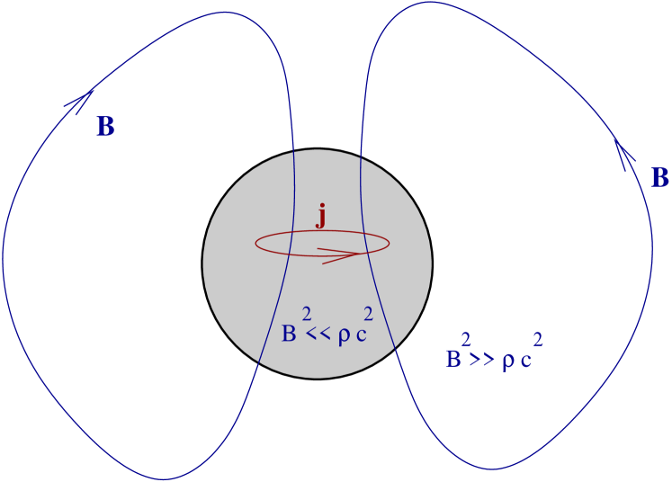
Figure 3: Magnetic ”phase separation” near the central source. The currents supporting the strong magnetic field flow in the matter dominated phase inside the neutron star (or in the accretion disk in case of BH-torus system). The outside corona is magnetically dominated (cf. the Sun).

As the momentum is carried primarily by electromagnetic field, the baryon loading can be negligible. However, it clearly cannot be too large. This imposes constraints on the amount of initial loading and entrainment within a stellar envelope. In analogy with the Sun one may expect that there are two “phases” within a source: an internal matter-dominated one in which large currents are flowing and an external magnetically-dominated (see Fig. 3). If a flow is launched from the magnetically-dominated phase the matter loading may be expected to be small (analogous to pulsar wind).

5. Where are the thermal precursors?

The intensity of the thermal precursor is set by the degree of lepto-photonic loading which can be arbitrarily small (Lyutikov & Usov, 2000; Daigne & Mochkovitch, 2002). A small precursor seen by Frontera et al.  (2001) indeed had very small luminosity.

6. How are particles accelerated at relativistic shock fronts?

As we discuss further in Paper II, the particle acceleration for the GRB does not take place at a relativistic shock front but is instead due to magnetic field dissipation in the emission region. Electromagnetic energy is “high quality”: it can be effectively converted into high frequency electromagnetic radiation. For example, in case of Solar flares, the primary energy output is non-thermal electrons Benz et al.  (2003). The particle acceleration that leads to afterglows may be shock-related but could also be due to relativistic MHD modes.

7. How is the magnetic field amplified?

The electromagnetic field is already present and provides the dominant energy density during GRB emission. In addition, we suppose that, during the afterglow, the magnetic field is supplied by the magnetic shell and may be incorporated into the shocked circumstellar gas through interchange instabilities (e.g. impulsive Kruskal-Schwarzschild instability appendix D) or due to resistive instabilities of the contact surface.

8. How is a large degree of $\gamma$-ray polarization created?

A strong argument in favor of electromagnetic models comes from the recent report of large polarization in RHESSI  observations of the prompt $\gamma$-ray emission from one GRB (Coburn & Boggs, 2003). If high polarization is substantiated and found to be generic, it would imply that the magnetic field coherence scale is larger than the size of the visible emitting region, $\sim r/\Gamma$. Such fields cannot be generated in a causally-disconnected, hydrodynamically-dominated outflow. Thus, the large scale magnetic field should be present in the outflow from the beginning and is likely to be the driving mechanism of the explosion (Lyutikov et al. , 2003).

9. What determines the jet opening angle and its structure?

GRB outflows have large opening angles, but do not have a jet in a proper sense. Outflows are non-isotropic so an achromatic break is inferred when the viewing angle is $\sim 1/\Gamma$. The jet internal structure corresponds to a ”structured jet” with $L_{\theta}\sim\theta^{-2}$.

10. What is the relation between GRBs and X-ray flashes (XRFs)?

GRBs are seen from essentially all directions in the electromagnetic model. XRFs are GRBs seen ”from the side”. The typical total energy (inferred from observations of early afterglows) should be similar to GRBs (within an order of magnitude). In the only XRF with a redshift this is indeed the case (Soderberg et al. , 2003). In a flux- or fluence-limited survey, the bursts viewed at large observer inclination should be systematically closer.

11. Where are the “orphan” afterglows?

Since in the electromagnetic model GRB outflows have large opening angles the incidence of orphan afterglows should be much less than in the fireball model.

There are other appealing features of the electromagnetic model. (i) The sources that are invoked are very similar to known sources. Pulsar wind nebulae, magnetars and extragalactic jets (as well as, perhaps, Galactic jets) are explained as low entropy outflows associated with spinning, magnetized, neutron stars, black holes and relativistic disks. What is novel about the GRB is the combination of high field and spin in a stellar object. (ii) Variability may be due to the statistical properties of dissipation and not the central source activity. Magnetic fields are non-linear dissipative dynamical system which often show bursty behavior with power law PDS. (iii) “Standard candle” - the narrow distribution of GRB energies (inferred from prompt emission, Frail et al.  (2001), from afterglows, Panaitescu & Kumar (2002), and from $K_{\alpha}$ lines, Lazzati et al.  (2002)) may be related to the total rotational energy of a critically rotating relativistic object - a one parameter (mass) family. (iv) Correlations of GRB properties: hard-to-soft temporal evolution of GRB spectra and $E_{\rm peak}\propto\sqrt{L}$ correlation naturally occur in the model (see section 11).

3.3 GRBs as electromagnetic circuits

The electromagnetic model exhibits some simple generalities that derive from treating it as a circuit. Suppose that the source is threaded by a magnetic flux, $\Phi\sim B_{s}r_{s}^{2}\sim 10^{26}$ G cm², and has a typical angular velocity $\Omega\sim 10^{4}$ rad/s^-1. The source will generate an EMF, $V$, and an associated current, $I$

$${\cal E}\sim\Omega\Phi\sim 3\times 10^{22}B_{s,14}r_{{\rm s,6}}\sim\sqrt{4\pi L\over c}\sim 3\times 10^{22}L_{50}^{1/2}\ {\rm V}.$$ (3)

There will be an associated current

$$I\sim{\cal E}/{\cal Z}_{\rm load}\sim\sqrt{Lc\over 4\pi}\sim 3\times 10^{20}B_{s,14}r_{{\rm s,6}}\sim 3\times 10^{20}L_{50}^{1/2}\ {\rm A},$$ (4)

where $B_{{\rm s}}=10^{14}B_{{\rm s,14}}\ {\rm G}$ is the source magnetic flux density and ${\cal Z}_{\rm load}\sim 100\,\Omega$ is the total impedance of the source and the emission region, which is of order the impedance of free space under general electromagnetic and relativistic conditions. The source region can be thought of as a generator capable of sustaining an EMF $\cal E$. (Under most conditions the maximum energy to which a particle of charge $Z$ can be accelerated will be limited by $\sim Ze{\cal E}\sim 3\times 10^{22}$ eV, way above the highest energy of the observed cosmic rays of $3\times 10^{20}$ eV.) This implies that the power dissipated in the load is $L\sim{\cal E}^{2}/{\cal Z}_{{\rm load}}$. The load consists of external medium, against which $PdV$ work is done by the expanding shell, and radiation (some of the energy of the shell is radiated away as a prompt emission). An equivalent and useful way to think about this is to say that there is a strong, quadrupolar current distribution outward along the axes and inward along the equator (or vice versa). Our proposal differs from the conventional interpretation principally through the assumption that the current flows all the way out to the expanding blast wave, rather than completes close to the source (c.f. Fig. 2).

We now consider, in more detail, the dynamics of the expansion. We divide the explosion into four phases, source formation ($t<<t_{s}$), bubble inflation ($r_{s}/c<<t\mathrel{\raise 1.29167pt\hbox{$<$}\mkern-14.0mu\lower 2.58334pt\hbox{$\sim$}}t_{s}$), shell expansion ($t_{s}\mathrel{\raise 1.29167pt\hbox{$<$}\mkern-14.0mu\lower 2.58334pt\hbox{$\sim$}}t\mathrel{\raise 1.29167pt\hbox{$<$}\mkern-14.0mu\lower 2.58334pt\hbox{$\sim$}}r_{{\rm GRB}}/c$ and blast wave propagation ($r_{{\rm GRB}}/c\mathrel{\raise 1.29167pt\hbox{$<$}\mkern-14.0mu\lower 2.58334pt\hbox{$\sim$}}t$). Each of these phases involves distinct, dynamical behavior requiring different approximations to describe.

4 Source Formation

4.1 Nature of the Compact Object

As explained above, there is now good circumstantial evidence linking at least some GRBs with simultaneous supernova explosions – the collapsar model. In its original and most common form, (e.g.  Woosley, 1993), it is supposed that the core collapse of a massive star leads to the formation of a massive black hole orbited by a dense, thick accretion disk It is also assumed that magnetic flux is generated locally by dynamo action (e.g.  Thompson & Murray, 2001). The actual power may derive from the spinning spacetime of the black hole or at the expense of the binding energy of the orbiting gas. For a rapidly spinning hole of mass $\sim 10$ M_⊙, a field of strength $B_{s}\sim 10^{14}L_{50}^{1/2}$ G suffices in either case. The simplest descriptions of these processes comprise solutions of Maxwell’s equations in a curved spacetime under the force-free approximation. They describe, at least conceptually, a stationary, axisymmetric flow of electromagnetic energy and angular momentum away from the surface of the hole and the disk. There is an associated current distribution that is quadrupolar so that the sign of the radial component of the current changes with latitude.

Real source is unlikely to be either stationary or axisymmetric. The field configuration may well be unstable and irregularities in the disk will break the symmetry. Our fundamental assumption, that underlies most of what follows, is that these instabilities do not develop to large nonlinear amplitude and completely disrupt the outflow. In other words, the large scale field is simple and approximately axisymmetric beyond the light cylinder. This large scale regularity can come about either because the smaller scale magnetic structure is erased through dissipation or, in the case of a central neutron star, through a topology-preserving re-arrangement of the magnetic flux. Our “DC” model is therefore rather different from other “AC” proposals that GRBs be powered by a rapidly varying Poynting flux (e.g.  Lyutikov & Blackman, 2000; Spruit et al. , 2000; Sikora et al. , 2003).

In the magnetar model, it is proposed that the neutron star is born with a rotation frequency $\sim 3L_{50}^{1/2}t_{s2}^{1/2}$ kHz and a dipole field of strength $B_{s}\sim 10^{14}L_{50}^{-1/2}t_{s2}^{-1}$ G so that it can produce the inferred, electromagnetic power and energy. If the dipole is inclined with respect to the rotation axis, we expect that some of the open magnetic flux from the northern magnetic pole finds its way into the southern hemisphere beyond the light cylinder and vice versa. Adopting our conjecture, provided that the dipole is not too inclined, the asymptotic electromagnetic configuration is roughly axisymmetric with field lines ending up in the hemisphere from which they started. In other words, the corrugations in the current sheet that separates the north seeking and south-seeking field lines smooth out, with little dissipation, close to the light cylinder. Much of what follows is predicated on this hypothesis, that a large scale quadrupolar current flow is established and provides a good description of the subsequent evolution of the bubble and the shell (e.g.  Blandford, 2002).

In the immediate vicinity of the source the plasma is separated into two phases: matter-dominated and magnetically dominated (c.f., Solar photosphere, pulsar magnetospheres). Superstrong magnetic fields are generated in the dense medium (a disk or a differentially rotating neutron star-like object). Buoyant magnetic field lines emerge into the tenuous magnetosphere while remaining anchored in the matter-dominated phase. Strongly relativistic outflow is generated in the magnetically dominated phase.

Although the magnetosphere is comparatively small, the electrodynamical conditions at the light cylinder constitute a boundary condition for the eventual, relativistic outflow, much like what happens with vacuum electromagnetic radiation. We can think of these conditions either as establishing the current distribution or, equivalently, as defining the subsequent evolution of the electromagnetic field. As the source will, typically, remain active for $\sim$ million dynamical times, we suppose that it will be able to settle down quickly to a quasi-steady state evolving slowly as the hole or neutron star slows down on a time scale of $\sim$ 100 s.

4.2 Dissipation at the Source, $r\sim r_{s}$

In any scenario some fraction of the central source luminosity is likely to be dissipated close to the source. In other words, there is a source impedance ${\cal Z}_{s}$. In the case of electromagnetic extraction of energy from a spinning black hole, this dissipation occurs beyond the event horizon. For a magnetar, the neutron star impedance is negligible and ${\cal Z}_{s}$ is dominated by what happens in the magnetosphere. In the fireball model, it is implicitly assumed that all of the energy released is quickly converted into heat, forming a high entropy per baryon, thermal plasma. In other words, the load impedance ${\cal Z}_{L}$ is located close to the source. By contrast, in the electromagnetic model this does not happen and the energy flows way from the light cylinder mainly in the form of an electromagnetic Poynting flux and the load impedance is located in the emission region. We argue that this is likely to be the case because, somewhat paradoxically, it becomes harder to convert electromagnetic energy directly to pair plasma the stronger the magnetic field becomes. The reason is that the plasma surrounding the source is highly conductive. In such plasma there is usually plenty of charge available to screen the component of the electric field along the magnetic fields, so that the first electromagnetic invariant is close to zero: ${\bf E}\cdot{\bf B}\sim 0$ (the perpendicular component of the electric field just defines a plasma velocity as long as $E<B$, see below).

In strongly relativistic plasmas, a possible source of (inertial) resistivity is related to the break down of the ${\bf E}\cdot{\bf B}\sim 0$ approximation in cases when the real charge density falls below some critical value. In the case of rotating magnetic field, this minimum charge density needed to short out the component of electric field along the magnetic field is known as the “Goldreich-Julian” density

$$n_{GJ}={{\bf\Omega}\cdot{\bf B}\over 2\pi ec}\sim 10^{17}\mbox{cm${}^{-3}$}$$ (5)

The minimum energy density associated with this amount of plasma is $n_{GJ}mc^{2}$. It is convenient to introduce a parameter $\sigma$ as the ratio of the magnetic energy density $u_{B}={\bf B}^{2}/8\pi$ to the total plasma energy density $u_{p}$ including photons ($u_{p}$ has contributions from rest mass of ions and pairs plus internal energy)

$$\sigma={u_{B}\over u_{p}}$$ (6)

If the energy density $u_{p}$ is dominated by leptons with density given by Eq. (5), then the ratio (6) is roughly the ratio of the light cylinder radius to the electron gyro radius which can be as large as $\sim 10^{18}$.

A conservative flow of plasma may not be able to satisfy the constraint that the local charge density always exceeds $n_{GJ}$. If this happens, a gap will develop where the field-aligned electric fields are nonzero ${\bf E}\cdot{\bf B}\neq 0$. However, the maximum potential drop that is available for dissipation will be limited by various mechanisms of pair production. Typically, after an electron has passed through a potential difference $\Delta V\sim 10^{9}-10^{12}$ V it will produce an electron-positron pair either through the emission of curvature photon or via inverse Compton scattering. This will be followed by an electromagnetic cascade and the newly born pairs will create a charge density that would shut-off the accelerating electric field. The typical potential difference required for the creation is orders of magnitude smaller than the total available EMF ${\cal E}\sim 10^{22}$ V. In this case the magnetization parameter may be estimated as

$$\sigma\sim{{\cal E}\over\Delta V}\sim 10^{10}$$ (7)

Another possible way through which an electromagnetically-dominated flow can create entropy directly and reduce $\sigma$ appreciably is through the development of an electromagnetic turbulent cascade operating down to wavelengths, $\lambda_{{\rm min}}$, so small that electromagnetic energy can be dissipated directly in particle acceleration. This is analogous to the viscous dissipation that terminates a fluid turbulence spectrum. If this really can operate then it is hard to see how more than a few percent of the electromagnetic energy will be dissipated in this fashion. More specifically, for a differential cascade a typical cascade time is the interaction time multiplied by the logarithm of the outer and inner scale (Zakharov et al. , 1992). If the typical interaction time is a light crossing time, then we can estimate $\sigma\sim\ln(r_{s}/\lambda_{{\rm min}})\sim 100$ (where $\lambda_{{\rm min}}$ of the order of Larmor radius), so that the flow will remain electromagnetically dominated.

Another source of dissipation is magnetic reconnection. This is surely important if the outflow retains an AC component, contrary to our hypothesis, or if current sheets develop as a result of the nonlinear evolution of electromagnetic instabilities. Driven relativistic reconnection may proceed at velocities approaching the speed of light (Lyutikov & Uzdensky, 2003), however the initial development of dissipative current sheets occurs on a timescale intermediate between very long resistive and very short dynamic (light travel) timescale and may be too slow to dissipate much of the magnetic energy density (Lyutikov, 2003a).

Thus, an abundance of pairs can be created without changing the electromagnetic dominance and the more pairs are present, the harder it becomes to create the small “gaps” that would be necessary to replenish them. Put another way, the pair density required to supply the electrical current and space charge scales linearly with the field strength, while the electromagnetic energy density scales as its square. The stronger the field, the more likely it is to persist into the outflow. It is because GRBs are so powerful that the dissipation in the source is probably low.

5 Bubble Inflation, $r\leq ct_{s}$

In the previous section we have argued that the flow formation occurs on a scale of a light cylinder, $r\sim r_{s}\sim 10^{6}$ cm and that the dissipative processes are not likely to drain all the potential EMF, so the flow is likely to remain magnetically-dominated. The velocity with which the plasma leave the neighborhood of the light cylinder is determined by the details of the acceleration and magnetic field structure at the source. For the purpose of this paper we leave the question of the detail structure of the central source open, assuming that the formation of the flow occurs in a way similar to pulsar magnetospheres (Michel, 1969; Goldreich & Julian, 1970), with an important difference – in GRBs pressure effects may play an important role. Beyond the light cylinder the magnetized flow generated by the central source will expand due to magnetic and pressure forces (see also Wheeler et al. , 2000; Moiseenko et al. , 2003). It will become super-fast-magnetosonic and thus causally disconnected from the source (Goldreich & Julian, 1970). For subsequent evolution the conditions close to source may be considered as boundary conditions at which the rate of energy and magnetic flux injection is some given function.

The asymptotic structure (at $r\gg r_{s}$) of axisymmetric, magnetized outflows is a challenging problem that has a considerable literature (e.g.  Heyvaerts & Norman, 2003, and references therein). Heyvaerts and Norman argue that a perfect, non-relativistic MHD flow with five conserved constants of the motion evolves either to a state where the current is confined to the axis and a finite number of thin current sheets or that the current closes and that the outflow energy flux becomes purely mechanical (for relativistic flows the latter happens at distances much larger than astrophysically relevant scales). In the context of a quadrupolar current distribution, the first option is equivalent to stating that the current becomes concentrated on the axis, surface and equator. They also argue that the second possibility is ultimately favored but that finite flows may not, in practice, achieve this state. .

As the wind expands, it starts to interact with the surrounding medium, so that its properties are determined both by initial conditions and interaction with the surrounding medium. The wind is slowed down by interaction with the stellar material, so that initial expansion is non-relativistic, and later, after breakout, it becomes strongly relativistic. The physical processes governing these two phases are quite distinct. We consider them in turn.

5.1 Non-relativistic expansion

Consider a newly-formed, compact object inside a star or other dense gas distribution generating an EMF ${\cal E}(t)$ and driving a quadrupolar current flow $I(t)$ as described above. This will inflate an electromagnetic bubble expanding at a rate controlled by the external gas density. Let the bubble radius be $R(\theta,t)$ where $\theta$ is the polar angle measured from the symmetry axis defined by the spin of the compact object. For the moment, suppose that the bubble expands non-relativistically.

We expect magnetic flux (integrated over the meridional plane) to cross the light cylinder and be supplied to the bubble at a rate $\dot{\Phi}\sim\mu_{0}Ic/2\pi$. Similarly, Poynting flux will be supplied to the bubble at a rate $\dot{U}_{{\rm EM}}\sim{\cal E}I$ . We can also compute the magnetic flux $\Phi={\cal L}I$ and the energy stored within the bubble $U_{{\rm EM}}={\cal L}I^{2}/2$, using the self inductance ${\cal L}$. If, as we discuss further below, the magnetic field in the bubble is predominantly toroidal between cylindrical radii $\varpi_{{\rm min}}$ and $\varpi_{{\rm max}}=R\sin\theta$, this is given by

$${\cal L}\sim{\mu_{0}\over 2\pi}\int dz\ln\left({\varpi_{{\max}}\over\varpi_{{\rm min}}}\right).$$ (8)

We therefore see that, if the bubble expands homologously and sub-relativistically, the rate of supply of both flux and energy exceeds the rate at which the flux and energy can be stored by a factor $\sim[\ln(\varpi_{{\rm max}}/\varpi_{{\rm min}})(dz/dt)/c]^{-1}$ (cf.  Rees & Gunn, 1974). Therefore, too much flux and energy is generated by the source when the expansion speed is less than $\sim 0.1c$.

The fate of this surplus flux and energy depends upon the amount of dissipation within the bubble. If, despite strong driving, the resistance in the electrical circuit is sufficiently low (much less than $\sim 100\Omega$), then the electromagnetic energy would be either reflected back to the source changing its properties (this can and does happen with solid conductors, e.g. waveguides, but is unlikely to happen in a plasma environment), or there will be “inductance breakdown”, so that ${\cal L}$ will decrease below the estimate (8). This will be achieved by destroying axial symmetry of the flow by MHD instabilities and creation of smaller scales current, much along the lines of what has been suggested in the Crab Nebula by Begelman (1999). On the other hand, if the resistance in the electrical circuit is sufficiently high, magnetic flux and electromagnetic energy will flow toward those parts of the current flow where the resistance is located. Magnetic energy then can be dissipated at a very high rate (this is similar to the case of driven magnetic reconnection, which in relativistic plasma may proceed at the speed approaching a speed of light (Lyutikov & Uzdensky, 2003)). The total electrical resistance needed can be estimated from the ratio of the potential difference at the light cylinder to the current as $\sim 60\Omega$ times a logarithmic factor and we will estimate the total resistance as $100\Omega$. In this paper, we assume that the current flows out to the boundary of the bubble and the Poynting flux is transformed into heat until the expansion speeds exceeds $\sim 0.1c$. Thereafter, it can be accommodated non-dissipatively by the expanding, electromagnetic bubble.

However, if the resistance in the outer part of the bubble always exceeds $\sim 100\Omega$, then the current will complete closer to the compact object and the outer parts of the bubble will comprise hot radiation/pair-dominated plasma. This is the implicit assumption underlying fireball models of GRBs that invoke electromagnetic sources.

As mentioned above, ideal MHD flows are naturally collimating. At the non-relativistic stage of expansion there is another collimating effect due to resistive dissipation, which, as we have argued, must be present in the flow. Most of the dissipation is likely to occur near the axis where the current density is highest and the susceptibility to known instability is the greatest. In this case a lateral flow of energy will set in carrying the poloidal field lines with it towards the axis (dissipation of magnetic energy on the axis will result in a loss of magnetic pressure, which resists the inflow of plasma towards the axis, and will be communicated to the bulk of the flow by a rarefaction wave propagating away from the axis). This, in turn, will leads to the pile-up of magnetic field near the axis and to faster radial expansion (the toothpaste tube effect).

Next we consider the structure of the axial current, whose radius $\varpi_{{\rm min}}$ we have already introduced. If the energy that is dissipated were to be radiated immediately and to escape freely, then the field structure would evolve to become force-free everywhere. This would imply that $\varpi_{{\rm min}}\sim r_{s}$, the radius of the light cylinder. However, this is surely not the case. The optical depth of the plasma will be far too large and the radiation will be trapped and thermalize. This implies that pressure is likely to become quickly important in the core. For $r>>r_{s}$, the net poloidal field is quite small. The simplest structure to consider is that of a Bennett pinch. In a Bennett pinch, the internal energy associated with the plasma is $3\mu_{0}I^{2}/16\pi$ per unit length so that the mean value of $\sigma$ is $4\ln(\varpi_{{\rm max}}/\varpi_{{\rm min}})/3$. A substantial plasma energy density is needed to oppose the magnetic stress independent of the choice of $\varpi_{{\rm min}}$. However Bennett pinches are notoriously unstable and so this is also unlikely to be a complete description of the current. The instabilities that would develop within the core lead to a less ordered and dynamic magnetic field with pair plasma contributing to the overall stress tensor to an extent controlled by the balance between its rate of creation and annihilation which we discuss below. Furthermore, we suppose that these instabilities lead to dissipation and that the effective impedance in the circuit automatically adjusts to match that required to account for the electromagnetic energy and flux supplied by the source at the light cylinder and the rate of expansion of the bubble.

In summary, we adopt a particularly simple distribution of currents generated by the central source: along the axis, the surface of the magnetic bubble and closing in the equator. More general current distribution do not change the picture qualitatively, but will lead to quantitative changes in our conclusions.

5.2 Dynamics of magnetic bubble inside a star

Electromagnetic bubbles are crucially different from expanding fireballs in another way. They are naturally self-collimating and will create bipolar outflows even if the stellar mass distribution is spherically symmetric.

The dynamics of such non-spherically expanding bubble may be described using the method of Kompaneets (1960) which was initially developed for propagation of non-spherical shocks (for astrophysical applications see Icke, 1988; Bisnovatyi-Kogan & Silich, 1995). Consider a small section of non-spherical non-relativistically expanding CD with radius $R(t,\theta)$. The CD expands under the pressure of magnetic field so that the normal magnetic stress at the bubble surface is balanced by the ram pressure of the surrounding medium. At the spherical polar angle $\theta$ the CD propagates at an angle

$$\tan\alpha=-{\partial\ln R\over\partial\theta}$$ (9)

to the radius vector. Balancing the pressure inside the bubble $B^{2}/(8\pi)=I^{2}/(2\pi c^{2}R^{2})$ with the pressure of the shocked plasma we find

$$\left({\partial R\over\partial t}\right)^{2}_{\theta}=\kappa{I^{2}(t)\over 2\pi R^{2}\sin^{2}\theta\rho(R,\theta)}\left[1+\left({\partial\ln R\over\partial\theta}\right)^{2}_{t}\right]$$ (10)

where $\kappa$ is a coefficient of the order of unity which relates the pressure at the CD to the pressure at the forward shock.

Equation (10) shows that non-spherical expansion inside the star is due both to the anisotropic driving by magnetic fields and collimating effects of the stellar material (the term in parenthesis, which under certain conditions tends to amplify non-sphericity). Note that this use of the Kompaneets approximation assumes that the shock and the CD are located close enough so that there is no lateral (in $\theta$ direction) redistribution of pressure in the shocked material. This is a good approximation for accelerating shocks and is used here only to illustrate qualitative behavior of the solutions.

The rate of expansion of the bubble inside the star depends upon the dynamics of the stellar envelope and the time evolution of the current $I(t)$. For a given dependence $\rho(R,\theta)$ and $I(t)$ Eq. (10) determines the velocity of the CD. Generally solutions will be strongly elongated along the axis. A simple analytical solution for $I,\,\rho\sim const$ is

$$R(t,\theta)=\left({2\over\pi}{I^{2}\over\rho c^{2}}\right)^{1/4}{\sqrt{t}\over\sin\theta}.$$ (11)

(current is related to the luminosity by Eq. (4). Qualitatively, the bubble and the forward shock will cross the iron core ($r_{c}\sim 2.5\times 10^{8}$ cm) in $t\sim r_{c}\sqrt{\rho}/B(r_{c})\sim.3$ sec, short enough to produce an ample supply of ${}^{56}Ni$ Woosley et al.  (2003). If we define $M(R)$ as the stellar mass external to radius $R$, then we can also estimate the breakout time

$$t_{{\rm breakout}}(\theta)\sim{1}\theta_{-1}^{2}\left({M\over M_{\odot}}\right)^{1/2}\left({R\over R_{\odot}}\right)^{1/2}L_{50}^{-1/2}~{}{\rm s}$$ (12)

The electromagnetic bubble can be confined equatorially by the star for the duration of the burst $t_{{\rm breakout}}(\pi/2)\sim 100$s and will expand non-relativistically as we have assumed. However the expansion along the axis proceeds on a short timescale and breakout should occur early in the burst. Furthermore, at the time of breakout, the axial expansion speed of the bubble will become relativistic.

Non-relativistic expansion lasts for several seconds along the axis. This time is much shorter than the burst duration. Recall that when the velocity of expansion is $\leq 0.1$, a considerable fraction of the magnetic energy is indeed dissipated. But since the flow quickly becomes relativistic, the relative fraction of dissipated energy is small, so that the flow magnetization remains large, $\sigma\geq 100$. An important advantage of the electromagnetic models is that as long as $\sigma\geq 1$, the asymptotic evolution of the flow is mostly independent of $\sigma$. Most of the dissipation described above will result in creation of lepto-photonic plasma, which decouples after photosphere, so that the remaining flow remains strongly magnetized. For $\sigma\geq 1$ the energy associated with the thermalized component is not important for the flow dynamics.

In summary, our contention is that, initially, when the bubble expands non-relativistically, the dissipation is concentrated along the pole and the current returns to the source along the surface of the bubble. The polar current pinch is supported against collapse at its core by a combination of plasma pressure and, possibly, by dynamical, disorganized magnetic field. After breakout, the expansion becomes relativistic and the resistance falls so that the electromagnetic energy that is still being supplied by the source is mostly absorbed by the inflating bubble and by doing work against the surroundings.

5.3 Early optically thick expansion: mini-fireball

In the previous subsection we have argued that energy release and initial non-relativistic stage of expansion are necessarily accompanied by partial dissipation of the magnetic energy, but the flow is likely to remain magnetically dominated with $\sigma\gg 1$. For any reasonable $\sigma\leq 10^{10}$ the lepto-photonic component will be optically thick near the central source and consequently in a thermodynamic quasi-equilibrium. In this subsection and in appendix A we discuss the optically thick, quasi-spherical expansion of a relativistically hot, magnetically-dominated flow after the flow became weakly relativistic and no further dissipation of magnetic energy is happening in the flow, but at the early enough stages so that photons remain trapped (see also Vlahakis & Königl, 2003a, b; Fendt & Ouyed, 2003, for a more extensive analysis).

Under the electromagnetic hypothesis, most of the energy released by the source comes out in the form of Poynting flux. However, as we argued above, there must be some dissipation that would lead to creation of a lepto-photonic component. In addition, some ions may be present in the flow. The luminosity of the source then can be written as

$$L=\int d\Omega\Gamma^{2}r^{2}\beta c\left(b^{2}/2+w\right)$$ (13)

where $w$ is plasma enthalpy, $b$ is a toroidal magnetic field in the plasma rest frame, $\Omega$ is a solid angle. The luminosity (13) includes contributions from the rest mass energy density of ions and pairs, their kinetic pressure and the trapped photon gas. At early stages the plasma enthalpy is strongly dominated by lepto-photonic plasma with a temperature

$$T\sim\left({L\over a\Delta\Omega r^{2}\beta c\Gamma^{2}(1+\sigma)}\right)^{1/4}$$ (14)

where $\Delta\Omega$ is a typical opening solid angle. (The magnetization parameter in this case is $\sigma=b^{2}/2/w$). For any reasonable values of $\sigma$ close to the source this temperature is high enough, so that pairs are freely produced. At breakout, $r_{breakout}\sim 10^{10}$ cm, plasma is moving weakly relativistically, $\Gamma\sim 1$, so that the temperature may still be high enough for plasma to be pair-dominated

$$T_{breakout}\sim 100\,{\rm keV}L_{50}^{1/4}\Omega_{-2}^{-1}\sigma_{2}^{-1/2}r_{breakout,10}^{-1/2}$$ (15)

At this point the flow will accelerate to relativistic velocities. Initially, the expansion is mostly pressure-driven, even in the strongly magnetized case. This results in dynamics qualitatively similar to the unmagnetized case. During outflow, the wind plasma accelerates $\Gamma\sim r$ while its density, pressure and temperature decrease $n\sim r^{-3}$, $p\sim r^{-4}$, $T\sim r^{-1}$. During the pressure-driven expansion the flow becomes superfast magnetosonic $\Gamma^{2}>\sigma$, while the magnetization parameter remains approximately constant (appendix A). (Note that the magnetization parameter is equal to the ratio of the Poynting to the particle fluxes. Since it remains approximately constant for quasi-spherical expansion, there is little transfer of energy between the magnetic field and the plasma at this stage for the assumed quasi-spherical geometry of the outflow.)

When the temperature falls below $\sim 10-20keV$, most of the pairs annihilate. This occurs at $r_{ph}\sim 10^{11}$ cm. This suddenly reduces the optical depth to Thomson scattering below unity. (Under certain conditions photons may remain trapped in the flow (Section 5.4 below, also Lyutikov & Usov, 2000). In this case, thermal driving by photon pressure continues, until the thermal photons escape.) As a result the lepto-photonic part of the flow decouples from the magnetic field and $\sigma$ increases by roughly seven orders of magnitude to $\sigma\sim 10^{9}$. By this time most of the thermal energy has been spent on accelerating the flow to $\Gamma\sim 10$. Beyond the photosphere, thermal photons propagate freely. The thermal radiation from the lepto-photonic component has a rest-frame temperature $T_{0}\sim 10-20keV$ times a boost due to the bulk motion. This thermal radiation, which should peak around $\sim 100$ keV may put constraints on the initial $\sigma$ (Lyutikov & Usov, 2000; Daigne & Mochkovitch, 2002). There are indications that the thermal precursor has been observed Frontera et al.  (2001), with intensity $\sim 1\%$ of the total burst intensity. This can be used to estimate the magnetization parameter below photosphere as $\sigma\sim 100$, so that beyond the photosphere $\sigma\sim 10^{9}$.

5.4 Thomson and pair production depths

Next, we consider conditions on the optical depth to Thomson scattering and pair production in electromagnetic models beyond the photosphere when the ejecta plasma is cold, collisionless (so that the number of pairs is conserved) and strongly magnetized ($\sigma\sim 10^{9}$). Under certain conditions, determined below, it may remain optically thick to Thomson scattering and to pair production.

Under the approximation above, the total energy is carried by the Poynting and particle fluxes (the latter includes a contribution from the pair rest mass and proton rest mass). If we neglect possible effects of pair production due to the dissipation of magnetic field, the magnetization parameter becomes

$$\sigma={{b}^{2}\over 4\pi c^{2}m_{\pm}n_{\pm}^{\prime}(1+\xi)}$$ (16)

where $\xi=m_{i}n_{i}^{\prime}/m_{\pm}n_{\pm}^{\prime}$ is the ratio of ion to pair mass fluxes. (In a standard fireballs, $\sigma=0$, and pair are dynamically unimportant $\xi\sim m_{p}/m_{e}$; for magnetized, pair-loaded flows , $\sigma\gg 1$, $\xi\leq 1$. ) The total energy flux then can be written as

$$L=\Gamma^{2}{b}^{2}r^{2}c{1+\sigma\over\sigma}\Delta\Omega$$ (17)

and we find that

$$n^{\prime}_{\pm}={L\over\Delta\Omega r^{2}mc^{3}\Gamma^{2}(1+\sigma)(1+\xi)}$$ (18)

Introducing the compactness parameter

$$l_{c}={L\sigma_{T}r^{\prime}\over\Delta\Omega\Gamma^{2}r^{2}mc^{3}}$$ (19)

where $r^{\prime}\sim r/\Gamma$ is the typical size of emission region in the rest frame, we find that the optical depth to Thomson scattering is

$$\tau_{T}={L\sigma_{T}r^{\prime}\over\Delta\Omega r^{2}mc^{3}\Gamma^{2}(1+\sigma)(1+\xi)}={l_{c}\over(1+\sigma)(1+\xi)}$$ (20)

In order to escape, we require that photons must have $\tau_{T}\leq 1$. This places a lower limit on the radius:

$$r>\sqrt{L\sigma_{T}r^{\prime}\over\Delta\Omega mc^{3}\Gamma^{2}(1+\sigma)(1+\xi)}$$ (21)

which under the assumption $r^{\prime}\sim r/\Gamma$ gives

$$r>={L\sigma_{T}\over\Delta\Omega mc^{3}\Gamma^{3}(1+\sigma)(1+\xi)}$$ (22)

Thus, for large magnetization, $\sigma>1$, even for pair dominated flow, $\xi\ll 1$ the ejecta become optically thin to Thomson scattering at

$$r>10^{8}(1+\sigma)_{9}^{-1}\Delta\Omega_{-2}^{-1}\Gamma_{2}^{{}_{3}}\,{\rm cm}$$ (23)

(For an electron-ion plasma $\xi=m_{p}/m_{e}$, so that for a given $\sigma$ the flow becomes optically thin at radii which are three orders of magnitude smaller than for a pair plasma.)

Next, we estimate the radius at which the optical depth to pair production falls below unity. Assume that most photons emerge with energy $E_{br}\sim 200$ keV. The optical depth to pair production then becomes

$$\tau_{\gamma-\gamma}=n^{\prime}_{\gamma}(E_{br})\sigma_{\gamma-\gamma}r^{\prime}={\epsilon_{\gamma}L_{\Omega}\over r^{2}\Gamma cE_{br}}{11\over 180}\sigma_{T}{r\over\Gamma}\Delta\Omega$$ (24)

where $\epsilon_{\gamma}$ is the fraction of the luminosity emitted in $\gamma$-rays, $\sigma_{\gamma-\gamma}=(11/180)\sigma_{T}$ is the cross-section for pair production by particles with power law spectrum (Svensson, 1997), and primes denote quantities measured in the outflowing frame.

Using the definition of the compactness parameter (19), we can write the optical depth to pair production (24) as

$$\tau_{\gamma}={11\over 180}\epsilon_{\gamma}\Gamma l_{c}{mc^{2}\over E_{br}}$$ (25)

This can be called photon compactness. Since $mc^{2}/E_{br}\sim 2$,

$$\tau_{\gamma}\sim 0.1\Gamma l_{c}$$ (26)

The condition $\tau_{\gamma-\gamma}<1$ gives

$$r_{\gamma-\gamma}>{11\over 180}{mc^{2}\over E_{br}}\epsilon_{\gamma}{L_{\Omega}\sigma_{T}\over mc^{3}\Gamma^{2}}=3\times 10^{16}\,L_{50}\,\Gamma_{2}^{-2}\,{\rm cm}$$ (27)

The ratio of $\tau_{T}$ to $\tau_{\gamma}$ may then be used to find the ratio of photons to electrons

$${n_{\gamma}^{\prime}\over n_{\pm}}\sim 0.1{\Gamma\sigma(1+\xi)}\gg 1$$ (28)

Thus, there are many more photons than electrons and the flows will first become optically thin to Thomson scattering, but will remain optically thick to pair production up to much larger distances. For strong magnetization, $\sigma\gg 1$ the flow will become Thomson thin right after breakout, while remaining optically thick to pair production up to $r\sim 10^{16}$ cm (Eq. (24)). Note that in the electromagnetic model pair production may play a more important role than in the hydrodynamic models since it can regulate the component of electric fields along magnetic field and control acceleration of pairs.

5.5 Magnetic acceleration and collimation in the relativistic regime

The behavior of magnetized winds depends both on the conditions at the source (e.g. the lateral distribution of the energy and magnetic fluxes) and on the subsequent dynamics. Since for $t<t_{s}$ the expansion is quasi-stationary, we can assume that, at this stage, the progenitor produces a steady relativistic wind. There is an extensive literature on acceleration and magnetic collimation of outflows from pulsars (Michel, 1971; Benford, 1984; Sulkanen & Lovelace, 1990; Begelman & Li, 1992; Fendt et al. , 1995; Bogovalov & Tsinganos, 1999; Lyubarsky, 2002) and from disks (Blandford & Payne, 1982; Lovelace et al. , 1987; Contopoulos & Lovelace, 1994; Camenzind, 1995; Fendt & Ouyed, 2003). (Unfortunately, even in the cleanest case of pulsar winds, the dynamics of relativistic MHD outflows remains an unsolved problem).

Magnetic outflows can be naturally self-collimating through the action of magnetic hoop stresses, $\propto B_{\phi}^{2}/4\pi$. Generally, this magnetic hoop stress is counterbalanced by the gas pressure and magnetic field gradients, so that the flow evolution (collimation or de-collimation) depends on this balance (e.g.  Heyvaerts & Norman, 1989; Chiueh et al. , 1991; Vlahakis & Königl, 2003a; Fendt & Ouyed, 2003). Collimation also affects the magnetization of the flow. For radially expanding flow, $\sigma$ remains constant since both the magnetic energy density and the plasma rest mass energy density scale as $\propto r^{-2}$, so there is no transfer of energy between them (in this case magnetic hoop stresses are exactly compensated by the gradient of magnetic energy density). Collimation (or decollimation) leads to transfer of energy from magnetic field to plasma (or vice versa).

An important property of ultra-relativistic outflows is that their motion is virtually ballistic, so that any collimation should be achieved close to the source where the flow is only mildly relativistic. This is a well-known problem for stationary pulsar outflows and in AGNs (e.g.  Begelman & Li, 1992; Bogovalov & Tsinganos, 1999). The reason for the weak collimation is that far from the source the gas pressure and the poloidal magnetic fields are unimportant and the magnetic stress $\propto B_{\phi}^{2}$ is almost exactly balanced by the oppositely directed electric stress $\propto\beta^{2}B_{\phi}^{2}$. Thus, the resulting stress is quite small $\propto B^{2}/\Gamma^{2}$ (e.g.  Bogovalov, 2001). Increasing the magnetic field strength does not help either, since in the strongly magnetized outflow the rest frame energy density is $\propto B^{2}$, the resulting lateral acceleration is independent of the magnetic field strength. A simple way to see this is to consider the MHD force balance equation in the $\theta$ direction (see Eq. (C3))

$$\partial_{t}[(w+b^{2})\gamma^{2}\beta_{\theta}]+{1\over{r\sin\theta}}\partial_{\theta}[\sin\theta(p+b^{2}/2)]-\cot\theta{{p-b^{2}}\over r}=0$$ (29)

Eq. (29) shows that typically on a flow expansion time $\beta_{\theta}\sim 1/\gamma^{2}\theta$. Thus for angles $\theta\geq 1/\gamma$ the lateral dynamics is frozen-out for ultra-relativistic flow. and the geometry of the outflow is likely to be determined in the acceleration region near the light cylinder.

One particular stationary outflow configuration contains a quadrupolar current flow concentrated close to the polar axis and the equator. This current distribution minimizes the total energy given a total toroidal magnetic flux and has been advocated in relativistic stationary winds (Heyvaerts & Norman, 2003). In a stationary wind, the return current flows at infinity from the pole to the equator; in case of electromagnetic explosions, the return current flows along the surface of the bubble - the contact discontinuity. The magnetic field in the bubble is inversely proportional to the cylindrical radius. In what follows, we adopt this particular current structure. Eventually, the problem of flow acceleration near the source (near the light cylinder of the progenitor) and collimation is likely to be solved by numerical simulations. At this moment there are no strongly relativistic numerical simulations that trace the flow evolution from the subsonic accelerations region, through the special points of the flow to asymptotic infinity.

There are two important exceptions to the application of these principles. First, as we discussed in Section 5.1, at the non-relativistic stage plasma pressure, poloidal magnetic field and tangled component of the magnetic field may be important in providing support against hoop stress inside the current regions. Secondly, at late times, $t\geq t_{s}$, the flow need not be in equilibrium since it changes on dynamical (light travel) time scale and, in addition, energy may flow towards the axis where it is dissipated and radiated as $\gamma$-ray emission.

The minimum size of the core region is the magnetic Debye radius

$$r_{D}=\sqrt{I\over 2\pi nec}$$ (30)

(for a given density $n$ and total current $I$ the relative drift of current-carrying particles in this case is of the order of the speed of light). Note that it is orders of magnitude larger than the light cylinder radius $\sim r_{s}$. The corresponding minimal angular size of the core region can be estimated if we use definition (16) to eliminate the density

$$\theta_{0}={r_{D}\over R}=\left({m^{2}c^{5}\sigma^{2}\Gamma^{2}\over Le^{2}}\right)^{1/4}\approx 10^{-3}L_{50}^{-1/4}\sigma_{9}^{1/2}\Gamma_{2}^{1/2}$$ (31)

A type of collimation that we envision in case of electromagnetic explosions is somewhat different from the conventional ”jet” model of AGNs and pulsars. We expect that large Poynting fluxes associated with explosive release of $\sim 10^{51}$ ergs are sufficient to drive a relativistic outflow over a large solid angle, so that during the relativistic stage the resulting cavity is almost spherical. But the Lorentz factor $\Gamma$ of the CD may be a strong function of the polar angle.

5.6 Quasistationary force-free outflow, $r\leq ct_{s}$

At small radii, $r_{ph}\leq r\leq ct_{s}$, the interaction with the circumstellar matter is not important, so that the flow may be considered as stationary. At this stage the poloidal magnetic field is small, flow is ultra-relativistic and moving ballistically. We can drive general equations governing the behavior of such flows. Although the flow may still be supersonic, so that matter inertia is important, in the asymptotic regions most important forces normal to the field are electromagnetic (Nitta, 1995; Heyvaerts & Norman, 2003).

Consider a simplified model problem of steady state force-free wind carrying only toroidal magnetic field. The time-independent force-free flows are described by the stationary Maxwell equations with time derivatives set to zero:

$${\rm curl}{\bf E}=0\mbox{}$$

$${\rm curl}{\bf B}={\bf j}$$ (32)

(factor $4\pi$ has been absorbed into definition of current density). From Eq. (5.6), it follows that the electric field is a gradient of a potential, ${\bf E}=-\nabla\Phi$, and

$${B\partial_{\theta}\sin\theta B\over\sin\theta}=\partial_{\theta}\Phi\Delta\Phi\mbox{}$$

$${B\partial_{r}rB\over r}=\partial_{r}\Phi\Delta\Phi$$ (33)

Eliminating $\Delta\Phi$ from eqns (33) we find

$${\partial_{r}rB\over r}\partial_{\theta}\Phi-{\partial_{\theta}\sin\theta B\over\sin\theta}\partial_{r}\Phi=0$$ (34)

Which means that electric potential is a function of total current enclosed within a magnetic loop at polar angle $\theta$:

$$\Phi\equiv\Phi(I)$$ (35)

The equation for the current $I(r,\theta)$ then becomes

$$-{4I\over\sin^{2}\theta r^{2}}+\Delta I{\Phi^{\prime}}^{2}+(\nabla I)^{2}\Phi^{\prime}\Phi^{\prime\prime}=0$$ (36)

This equation resembles closely the relativistic Grad-Shafranov equation (e.g.  Beskin, 1997). The main difference is that under assumption of zero poloidal field the conventional flux function loses its meaning. In the standard theory of the Grad-Shafranov equation, there is a poloidal field which is related to the derivative of the flux function. We replace the flux function with the current enclosed by a given field loop and treat this as an independent variable. Equation (36) is considerably simpler than the full relativistic Grad-Shafranov equation. It has one free function - distribution of electric potential that in the steady state determines uniquely the current distribution. In the steady state the plasma experiences radial and lateral drift with velocities

$$\beta={E_{\theta}\over B}=-\Phi^{\prime}\sin\theta\partial_{\theta}\ln\sqrt{I},\hskip 21.68121pt\lambda=-{E_{r}\over B}=\Phi^{\prime}r\sin\theta\partial_{r}\ln\sqrt{I}$$ (37)

For radial motion $\lambda=0,\,I=I(\theta)$, equation (36) gives

$$\partial_{\theta}\left(I(\theta)\sqrt{1-\beta^{2}}\right)=0$$ (38)

which can be integrated

$$I(\theta)\sqrt{1-\beta^{2}}=I_{0}\sqrt{1-\beta_{0}^{2}}$$ (39)

where $I_{0}$ is the axial current and $\beta_{0}$ is the ratio of the axial charge density per unit length to axial current. Note that condition $\beta<1$ requires $I_{0}\neq 0$. Thus, subluminal expansion along conical surfaces requires presence of a line current (see also Heyvaerts & Norman, 2003). Further solutions of this equation can be written down but will not be considered here.

6 Electromagnetic Formalism

6.1 Relativistic Force-free Electro-dynamics

The conventional method for handling relativistic, magnetized flows is to use the relativistic extension of regular, non-relativistic magnetohydrodynamics. Relativistic MHD (RMHD) is considerably more complicated. In the non-relativistic case the displacement current is neglected, $\partial_{t}{\bf E}\rightarrow 0$, and a charge neutrality is assumed, $\rho_{e}\rightarrow 0$. Both of these assumptions may be violated in relativistic plasmas. In addition, when calculating dynamic properties one needs to take into account the inertia of the electromagnetic field. However, there is a simpler extension, the relativistic force-free approximation (RFF), which is appropriate when the plasma is sufficiently tenuous and subsonically moving, so that its inertia can be ignored. On the other hand, the local microscopic plasma time scale (e.g. plasma frequency) typically is much shorter than the global dynamical time scales and there is plenty of charge available to screen the component of electric field along the magnetic field. In this case we can neglect the inertia of the plasma particles but have to include their electromagnetic interaction. This is relativistic force-free (RFF) approximation. (Inertial contributions may be included as perturbations to magnetic forces.)

There are two equivalent ways of deriving RFF equations. First, they can be derived from the two Maxwell equations (factor $4\pi$ has been absorbed into definitions of currents and charge densities):

$${\partial{\bf E}\over\partial t} = \nabla\times{\bf B}-{\bf j}$$ (40)

$${\partial{\bf B}\over\partial t} = -\nabla\times{\bf E}$$ (41)

with the current density perpendicular to the local magnetic field determined by the force-free condition,

$$\rho{\bf E}+{\bf j}\times{\bf B}=0$$ (42)

This immediately implies that the invariant ${\bf E}\cdot{\bf B}=0$ and its temporal derivative can be set to zero; in addition, electromagnetic energy is conserved, ${\bf E}\cdot{\bf j}=0$. This allows one to relate the current to the electro-magnetic fields

$${\bf j}={({\bf E}\times{\bf B})\nabla\cdot{\bf E}+({\bf B}\cdot\nabla\times{\bf B}-{\bf E}\cdot\nabla\times{\bf E}){\bf B}\over B^{2}}$$ (43)

This may be considered as the Ohm’s law for relativistic force-free electrodynamics.

For consistency of RFF, one also needs to assume that the second electromagnetic invariant is positive, $B^{2}-E^{2}>0$. This implies that there is a reference frame where the electric field vanishes Equivalently, the electromagnetic stress-energy tensor can be diagonalized. Note, that there is no mathematical constraint that would ensure that $B^{2}-E^{2}$ remains positive. Thus, even if initially $B>E$ everywhere, both numerical and analytical solution (e.g. Appendix F) may have regions where this condition becomes violated. The implies that the RFF is no longer valid, so that either plasma inertia or dissipation should be taken into account (Section 6.2).

The conditions ${\bf E}\cdot{\bf B}=0$ and $B^{2}>E^{2}$ allow us to define an electromagnetic velocity ${\bf v}={\bf E}\times{\bf B}/B^{2}$ perpendicular to the magnetic field. The velocity along the field is not defined. This degeneracy comes from a neglect of plasma dynamics associated with non-force-free motion of plasma along the field (however strong the magnetic field is, it does not influence the plasma motion along the field). Note, that under the force-free approximation all plasma species drift across the magnetic field with the same velocity. Thus, the current perpendicular to the magnetic field is exclusively due to the plasma charge density.

RFF equations (40-43) represents a simple evolutionary dynamical system (Uchida, 1997a; Komissarov, 2002), which can be solved numerically (e.g.  Komissarov, 2001). When one includes the constraints ${\bf E}\cdot{\bf B}=\nabla\cdot{\bf B}=0$, there are four independent electromagnetic variables to evolve and four characteristics along which information is propagated. In the linear approximation, these correspond to forward and backward propagating fast and intermediate wave modes with phase speeds $c$ and $c\hat{\bf k}\cdot\hat{\bf B}$ respectively ($\hat{\bf k}$ and $\hat{\bf B}$ are corresponding unit vectors).

RFF dynamics can be developed in a manner that is quite analogous to regular hydrodynamics, with the anisotropic Maxwell stress tensor taking the place of the regular pressure and the electromagnetic energy density playing the role of inertia (cf.  Uchida, 1997a; Komissarov, 2002). There is an important difference, though, in that the existence of a luminal fast mode means that electromagnetic “flows” do not become truly “supersonic” (see Section 6.2).

We would like to stress an important difference between non-relativistic and relativistic force-free fields: the relativistic force-free theory is dynamic. In laboratory (non-relativistic) plasma the notion of force-free fields is often related to the stationary configuration attained asymptotically by a system (subject to some boundary conditions and some constraints, e.g. conservation of helicity). This equilibrium is attained on time scales of the order of the Alfvén crossing times. In strongly magnetized relativistic plasma the Alfvén speed may become of the order of the speed of light $c$, so that crossing time becomes of the order of the light travel time. But if plasma is moving relativistically its state is changing on the same time scale.

6.2 Applicability of force-free approximation

Force-free electrodynamics assumes that the inertia of plasma is negligible. This approximation is bound to break down for very large effective plasma velocities, when electric field becomes too close in value to magnetic field, $E\rightarrow B$. The condition that inertia is negligible is equivalent to the condition that the effective plasma four-velocity, $u\sim E/(B\sqrt{1-(E/B)^{2}})$, is smaller that the Alfvén four-velocity in the plasma. In relativistic plasma

$$u_{A}^{2}={\sigma}$$ (44)

This puts an upper limit on the value of electric fields consistent with force-free approximation

$${B^{2}-E^{2}\over E^{2}}\gg{1\over\sigma}$$ (45)

A second constraint comes from the fact that in RFF the charge number density $n_{e}$ may be comparable to the total plasma number density $n$ and the current density may reach $j\sim nec$. Force-free electrodynamics assumes that there are enough charge carriers in the plasma to assure that the condition ${\bf E}\cdot{\bf B}=0$ is satisfied. This condition can be violated if the plasma density is too small and/or if fields change on very small scales (e.g. due to development of electromagnetic turbulent cascade which will bring energy to smaller and smaller scales). In this case plasma becomes charge-starved. To estimate charge-starved condition, assume that a typical fluctuating amplitude of magnetic field at the scale $l^{\prime}$ is $b_{l^{\prime}}$ (both quantities measured in the plasma rest frame). The corresponding current $j^{\prime}_{l^{\prime}}\sim cb_{l^{\prime}}/4\pi$ is limited by the number density of real charges $n^{\prime}$: $j^{\prime}_{l^{\prime}}\leq 2en^{\prime}c$, which gives (Thompson & Blaes, 1998)

$$n^{\prime}\sim{\delta b_{l^{\prime}}\over 2\pi el^{\prime}}$$ (46)

If this condition is violated, the electromagnetic perturbations behave more like electromagnetic waves than MHD waves. In particular, for smaller densities the condition ${\bf E}\cdot{\bf B}=0$ is not satisfied, so that electric fields can accelerate particles, which leads to dissipation of electromagnetic energy. This can be an important acceleration mechanism.

Thirdly, non-ideal effects (such as resistivity) may lead to violation of the ideal RFF approximation. It is possible to formulate equations of resistive RFF by introducing a macroscopic resistivity (Lyutikov, 2003a). In resistive RFF, the dynamics is still controlled by the electromagnetic field, but now the currents that support these fields may become dissipative. Resistive effects in magnetically-dominated plasma are somewhat different from the non-relativistic analog. In a force-free plasma, conduction currents only flow along the magnetic field in the plasma rest frame, so that only the component of current along the field is subject to resistive dissipation. Ohm’s law in resistive RFF becomes (Lyutikov, 2003a)

$$({\bf j}\cdot{\bf B})+\partial_{t}\left(\eta\sqrt{1-\left(({\bf E}\times{\bf B})/B^{2}\right)^{2}}({\bf j}\cdot{\bf B})\right)=({\bf B}\cdot\nabla\times{\bf B}-{\bf E}\cdot\nabla\times{\bf E}){\bf B}$$ (47)

In spite of the differences between resistive RFF and non-relativistic plasmas, effects similar to familiar resistive instabilities, like tearing mode, should develop in RFF (Lyutikov, 2003a). This has important implications for the numerical modeling of RFF fields: similar to fluid dynamics, where sound waves turn into shocks, RFF fields tend to form small scale structures in which resistive effects becomes important.

6.3 Relativistic force-free versus MHD

It is instructive to contrast this electromagnetic approach with the relativistic MHD (RMHD) formalism that is currently used by most investigators (e.g.  Phinney, 1982; Camenzind, 1986; Takahashi et al. , 1990; Takahashi, 2000; Park, 2002). In the RMHD formulation dynamic equations include inertial terms and pressure gradients. This means that a fluid velocity field must be tracked, along with enthalpy density and pressure. The electric field is supposed to be related to current and magnetic fields through an Ohm’s law. Under relativistic MHD, the constitutive relation, Eq. (43) must be augmented with inertial terms. The equations are still evolutionary, though more complex - there are seven independent variables to evolve, with seven independent wave modes (two fast, two intermediate, two slow and one adiabatic) to follow.

The introduction of these extra complications, when the inertia of the plasma is relatively small, can be questioned on several grounds. Firstly, it is assumed that the electric field vanishes in the center of momentum frame of the plasma. This is not guaranteed by plasma physics in a tenuous, relativistic plasma. Secondly, it is usually assumed that the plasma slides without friction along the magnetic field. In other words, there is no dissipation. This is unlikely to be the case in the face of instabilities and radiative drag (Beskin & Pariev, 1993). Thirdly, it is generally supposed that plasma is conserved. This is untrue in GRBs where pair creation may be important until far out in the outflow. Finally, there is the common assumption that the particle pressure tensor is isotropic. In practice this is rarely the case in observed plasmas. In contrast to that, the magnetic flux is a much better conserved quantity.

The relativistic force-free equations may be derived from relativistic MHD formulation in the limit of negligible inertia. This offers an advantage that the system of equations may be set in form of conservation laws and can be easily generalized to general relativistic form. The basic equations of RMHD include the relativistic Ohm’s law and the relativistic dynamics, Maxwell’s and mass conservation equations Lichnerowicz (1967); Uchida (1997a); Komissarov (2001):

$$T^{\mu\nu}_{;\nu}=0,$$ (48)

$$F^{\ast\,\mu\nu}_{;\nu}=0,$$ (49)

$$(\rho u^{\mu})_{;mu}=0$$ (50)

where the stress energy tensor is a sum of contributions from matter and fields:

$$T^{\mu\nu}=T^{\mu\nu}_{(m)}+T^{\mu\nu}_{(em)}\mbox{}$$

$$T^{\mu\nu}_{(m)}=wu^{\mu}u^{\nu}+pg^{ij}\mbox{}$$

$$T^{mu\nu}_{(em)}=F^{\mu}_{\alpha}F^{\nu\alpha}-{1\over 4}F_{\alpha\beta}F^{\alpha\beta}g^{\mu\nu}=b^{2}u^{\mu}u^{\nu}+{b^{2}\over 2}g^{\mu\nu}-b^{\mu}\,b^{\nu}$$ (51)

where $w$ is the plasma proper enthalpy, $\rho$ is proper plasma density and $p$ is pressure, $b_{\alpha}={1\over 2}\eta_{\alpha\beta\mu\nu}u^{\beta}F^{\mu\nu}$ are the four-vector of magnetic field, Levi-Civita tensor and electro-magnetic field tensor, $u^{\alpha}=(\gamma,\gamma{\bf\beta})$ are the plasma four-velocity, $F_{\mu\nu}$ is electromagnetic field tensor. An additional constraint is that the first electromagnetic invariant is zero:

$$F_{\mu\nu}\,^{\ast}F^{\mu\nu}=0$$ (52)

where ${}^{\ast}F^{\mu\nu}$ is a dual electromagnetic tensor.

It has been also implicitly assumed in the derivation of these equations that the second electromagnetic invariant $F_{\mu\nu}\,F^{\mu\nu}\neq 0$, so that the electromagnetic stress energy tensor can be diagonalized. This assumption is important since we are interested in the limit when matter contributions to the stress energy tensor vanish; the possibility of diagonalization of the electromagnetic stress energy tensor distinguishes MHD and vacuum electromagnetic fields where such diagonalization is not possible.

When we set the matter contributions to the stress energy tensor to zero, $w,p\rightarrow 0$, the RMHD equations become equivalent to the RFF equations with the exception that the velocity along the field is not defined anymore. This can also be checked by combining RFF equations in the form of conservation laws

$${1\over 2}\partial_{t}(E^{2}+B^{2})+\nabla\cdot\left({\bf E}\times{\bf B}\right)=0\mbox{}$$

$$\partial_{t}{\bf E}\times{\bf B}=\nabla\times{\bf B}\times{\bf B}+\nabla\times{\bf E}\times{\bf E}+(\nabla\cdot{\bf E}){\bf E}.$$ (53)

7 Relativistic expansion of the magnetic shell, $r>ct_{s}$

After breakout, the electromagnetic flow is accelerated by pressure and magnetic forces and becomes super-fast-magnetosonic. At the photosphere the lepto-photonic component decouples from the magnetic field, so that $\sigma$ increases to $\sigma\sim 10^{8}-10^{10}$, so that the wind becomes sub-fastmagnetosonic again. Beyond this point the outflow is strongly magnetically dominated and can be described by RFF equations. The wind is then further accelerated by magnetic pressure, while its expansion is determined by the interaction with external medium. In this section we study the dynamics of such magnetically-dominated explosions.

There are two principal differences between this work and other (mostly stationary MHD-type) approaches. First, the flow is commonly assumed to expand freely, without interaction with the circumstellar medium, so that the flow dynamics is determined by the internal structure of the flow. MHD flows usually cross fast magnetosonic critical surface after which they become causally disconnected from their source (Goldreich & Julian, 1970). A condition that the flow remains regular at the critical surface is what determines the global properties of the wind. Unlike MHD, force-free flows are sub-fastmagnetosonic so no conditions at the fast critical surface appear. In this case it is the interaction with boundaries that determines the properties of the flow (similar to subsonic hydrodynamic flows). In the case of freely expanding magnetized wind the terminal Lorentz factor $\Gamma_{\infty}$ depends very sensitively on details of geometry: for radially expanding MHD flows $\Gamma_{\infty}\sim\sqrt{\sigma}$ Michel (1969); Goldreich & Julian (1970). Thus, the distinctive feature between MHD and force-free flows is whether the wind becomes fast supersonic (MHD regime, $\Gamma>\sqrt{\sigma}$) or not (force-free regime, $\Gamma<\sqrt{\sigma}$). In case of GRB, beyond the photosphere $\sigma\sim 10^{9}$, so it the interaction of the force-free wind with the external medium (and not the internal wind dynamics) that is likely to limit acceleration to $\Gamma\sim 10^{4}$ (see below).

Secondly, the flows under consideration are strongly non-stationary, so that their dynamics is qualitatively different from stationary solutions and is more reminiscent of the strong explosion problem (Sedov, 1969). Relativistic effects introduce an important difference, though. Primarily, the differences lie in the causal structure of the shell. It takes a very long time for a wave to be reflected by the relativistically expanding surface of the shell (contact discontinuity) and return to the origin. This is generally true of ultra-relativistic flows so that stationary solutions, which take a long time to be established, can be quite misleading.

As we have discussed above the long time scales for establishing a ”feed-back” on the source have an important consequence for energy dissipation in the flow: there is no necessity to destroy magnetic flux through ohmic dissipation, until the wave can actually propagate back to the source. Stated another way, there need be little resistance in the electrical circuit. The effective load can consist of the performance of work on the expanding blast wave. This is where most of the power that is generated by the central magnetic rotator ends up. Thus, until the outflow becomes non-relativistic, the distinction between the inertial load and a different, dissipative load is quite unimportant for the behavior of the central source. As long as the expansion remains ultra-relativistic, it is a very good approximation to impose a Sommerfeld radiation condition on the solution at the source and to ignore the reflected wave.

The general problem of relativistic force-free expansion is quite complicated: we need to solve for the time-dependent, three-dimensional evolution of electric and magnetic fields with a non-linear coupling through the force-free Ohm’s law (43). (note that even normal modes in such plasma experience strong refractive phenomena). To make the problem tractable we make several simplifying assumptions. First, we limit our approach to distances much larger than the source scale $r_{s}$ and, since at large distances magnetic field is dominated by the toroidal fields, we neglect poloidal magnetic fields altogether (thus we also neglect the angular momentum loss by the source). Secondly, instead of treating the flow acceleration and collimation at the source, we assume that the central source can be represented as an inner boundary condition through which a toroidal magnetic flux is injected with a given total luminosity and a given polar angle dependence $L(\theta)$.

We assume also that at large distances, $r\geq r_{ph}$, the outflow may be described by ideal RFF equations. In this case the expansion of the relativistic shell will be subsonic, and virtually ballistic (radial). The energy input of the central source then can be represented as fast modes propagating from the source to the contact discontinuity. Motion of the CD is determined by the pressure balance between the Poynting flux from the source and the ram pressure of the ISM and thus depends on the source luminosity $L_{\Omega}(t^{\prime})$ per unit solid angle $d\Omega$ at the retarded time $t^{\prime}$ such that $R(t)=t-t^{\prime}$. Typically $R(t)/c\sim\Gamma^{2}t_{\rm source}$.

A particular form of the forward-propagating wave train (its temporal variations, amplitude and lateral distribution of the energy flux) depends on the history of the source activity and detailed properties of the source. Since the central source is expected to vary considerably during its activity, the pressure on the inner boundary of the CD will be fluctuating as the new pulses from the source start to contribute to the pressure. This will be reflected in the ”jitter” of the CD motion. At later times multiple reflections from the contact discontinuity and the center become important as well. As we have discussed in Section 5.5 the lateral distribution of the magnetic field and energy fluxes in the outgoing waves is likely to consist of a line current. Then, a very important observational consequence follows. For outgoing waves corresponding to the line current the distribution of Poynting flux is $L\sim 1/\sin^{2}\theta$, implying that the central source releases an equal amount of energy per decade of $\theta$. This would later translate into a similar form of the forward shock.

The form of the ingoing reflected wave depends both on the outgoing wave and the form of the contact discontinuity. Since in the strongly relativistic regime the wave will be reflecting from receding CD the amplitude of the reflected wave will be $\sim\Gamma^{2}$ times smaller.

The relativistic stage of the shell may be separated into two stages: ”coasting” and ”self-similar” depending on whether or not most of the fast waves emitted by the central source have caught up with the CD.

• “Coasting” electromagnetic shell ($ct_{{\rm s}}<r<r_{{\rm sh}}\equiv(L_{\Omega}t_{{\rm s}}^{2}/\rho c)^{1/4}$) (in the observer frame this phase lasts also $\sim 100$ s). At $r>r_{ph}$ the shell becomes a relativistically expanding shell of thickness $\sim ct_{{\rm s}}\sim 3\times 10^{12}t_{{\rm s,2}}\ {\rm cm}$. The shell still contains toroidal magnetic field but the current now detaches from the source and completes along the shell’s inner surface. At this stage the CD is constantly re-energized by the fast-magnetosonic waves propagating from the central source. The average motion of the CD is determined by the average luminosity, $\Gamma\sim(L_{\Omega}/\rho c^{3})^{1/4}r^{-1/2}$ (in a constant density medium) or $\Gamma\sim{\rm const}$ (in a $\rho\sim r^{-2}$ wind). In addition, there is a ”jitter” of the CD, in response to the ”jitter” in the source luminosity. The internal structure of the magnetic shell is a messy mixture of the outgoing waves from the source and the ingoing waves reflected from the CD, similar to a pre-Sedov phase in hydrodynamical explosions. Unlike the case of a hydrodynamic blast wave with energy supply, no internal discontinuities form inside magnetic shell.

• Self-similar electromagnetic shell ($r_{{\rm sh}}<r<r_{{\rm NR}}\equiv(L_{\Omega}t_{{\rm s}}/\rho c^{2})^{1/3}$). After one dynamical time scale, $t_{d}\sim\Gamma^{2}t_{s}\sim 3\times 10^{16}$ cm, all the regions of the shell come into causal contact – most of the waves reflected from the CD have propagated throughout the shell. As the expanding shell performs work on the surrounding medium its total energy decreases; the amount of energy that remains in the shell during the self-similar stage is small, $\sim E_{\Omega}/\Gamma^{2}$. Most of the energy is still concentrated in a thin shell with $\Delta R\sim R/\Gamma^{2}$ near the surface of the shell which is moving according to $\Gamma\sim\sqrt{E_{\Omega}/\rho c^{2}}\,r^{-3/2}$ (in a constant density medium), or $\Gamma\sim r^{-1/2}$ (in a $\rho\sim r^{-2}$ wind). The energy of the shell decreases only weakly with radius, $dE/dt\sim 1/r$ in constant density and $dE/dt\sim 1/r^{3}$ in a wind, so that the surface of the shell keeps moving relativistically as long as the preceding shock wave is moving relativistically, until $r\sim(E_{\Omega}/\rho c^{2})^{1/3}\sim 10^{18}$ cm - the shock never becomes completely free of the shell. Interestingly, the structure of the magnetic shell (in particular the distribution of energy) resembles at this stage the structure of the hydrodynamical relativistic blast wave (Blandford & McKee, 1976) (Section 8.1.1, m=3).

7.1 RFF equations for axisymmetric asymptotic flows

In the asymptotic domain $r\gg r_{s}$ the ejecta will be dominated by toroidal magnetic field and, since we assumed that all small scales field variations are smoothed out, it will be axially symmetric. In this case the only nonzero components of the fields are $B=B_{\phi},E_{r},E_{\theta}$ and the RFF equations (40) and (43) give

$$\partial_{t}B=-{1\over r}\partial_{r}(rE_{\theta})+{1\over r}\partial_{\theta}E_{r}\mbox{}$$

$$\partial_{t}E_{\theta}=-{1\over r}\partial_{r}(rB)+{E_{r}\over B}\left({1\over r\sin\theta}\partial_{\theta}(\sin\theta E_{\theta})+{1\over r^{2}}\partial_{r}(r^{2}E_{r})\right)\mbox{}$$

$$\partial_{t}E_{r}={1\over r\sin\theta}\partial_{\theta}(\sin\theta B)-{E_{\theta}\over B}\left({1\over r\sin\theta}\partial_{\theta}(\sin\theta E_{\theta})+{1\over r^{2}}\partial_{r}(r^{2}E_{r})\right)$$ (54)

The charge density associated with a given solution is given by

$$\rho={1\over r^{2}}{\partial_{r}(r^{2}E_{r})}+{1\over r\sin\theta}{\partial\over\partial\theta}E\sin\theta$$ (55)

and the currents are

$$j_{r}=\rho{E_{\theta}\over B}={E_{\theta}\over B}\left({1\over r^{2}}{\partial_{r}(r^{2}E_{r})}+{1\over r\sin\theta}{\partial\over\partial\theta}E\sin\theta\right)\mbox{}$$

$$j_{\theta}=-\rho{E_{r}\over B}=-{E_{r}\over B}\left({1\over r^{2}}{\partial_{r}(r^{2}E_{r})}+{1\over r\sin\theta}{\partial\over\partial\theta}E\sin\theta\right)$$ (56)

After some rearrangement the system (54) gives

$${1\over 2}\partial_{t}\left(E_{\theta}^{2}+E_{r}^{2}+B^{2}\right)+{1\over r^{2}}\partial_{r}r^{2}E_{\theta}B-{1\over r\sin\theta}\partial_{\theta}\sin\theta E_{r}B=0\mbox{}$$

$$\partial_{t}E_{\theta}B+{1\over r^{2}}\partial_{r}r^{2}\left(B^{2}+E_{\theta}^{2}\right)-{1\over r\sin\theta}\partial_{\theta}\sin\theta E_{r}E_{\theta}-{E_{r}\over r^{2}}\partial_{r}r^{2}E_{r}=0\mbox{}$$

$$\partial_{t}E_{r}B+{E_{r}\over r}\partial_{r}rE_{\theta}+{E_{\theta}\over r^{2}}\partial_{r}r^{2}E_{r}+{E_{\theta}\over r\sin\theta}\partial_{\theta}\sin\theta E_{\theta}-{B\over r\sin\theta}\partial_{\theta}\sin\theta B-{E_{r}\over r}\partial_{\theta}E_{r}=0$$ (57)

To connect to RMHD description we note that the plasma drift velocity is $(E_{\theta}/B){\bf\hat{e}}_{r}-(E_{r}/B){\bf\hat{e}}_{\theta}$. Setting $B=\gamma b,\,E_{\theta}=\beta\gamma b,\,E_{r}=\lambda\gamma b$ and the system (57) gives eqns (C6).

Equations (54) are the main equations that determine dynamics of the expanding magnetic shell.

7.2 Boundary condition on the contact discontinuity

To find the internal structure of the expanding magnetized shell the dynamical equations should be supplemented by boundary conditions on the contact discontinuity separating the relativistically expanding magnetic shell and external medium. The first boundary condition requires that the pressure of the magnetic field of the ejecta should be balanced by the pressure of the external medium. The pressure of the external medium is the ram pressure if the forward shock has not formed, or the kinetic pressure of the shocked material if the forward shock has formed. The two cases differ only by a numerical coefficient $\kappa$ (appendix B).

As the shell propagates into the surrounding medium it reflects particles with typical Lorentz factor $\sim 2\Gamma^{2}$. In the frame of the shell there must be a pressure equilibrium on the contact discontinuity. The magnetic pressure inside the shell, $B^{2}/(8\pi\Gamma^{2})$ should balance the ram pressure of the incoming external medium , $2\kappa\Gamma^{2}\rho_{\rm ext}c^{2}$, (here $\rho_{\rm ext}$ is the density of the external medium and $\kappa$ is a coefficient of the order of unity relating the ram pressure before the shock and kinetic pressure on the CD):

$$2\kappa\Gamma^{2}\beta^{2}\rho_{\rm ext}c^{2}={B^{2}\over 8\pi\Gamma^{2}}$$ (58)

where $B$ is the shell magnetic field measured in the lab frame. Thus, the magnetic field in the plasma rest frame should scale as $b\sim\Gamma$, while magnetic field in the lab frame scales as $B\sim\Gamma b\sim\Gamma^{2}$.

Alternatively, a force balance on the CD can be considered as a Lorentz force of magnetic field and the surface current acting against the ram pressure. Consider, for example, magnetic field occupying a half space $x>0$ and moving with velocity $\beta_{x}{\bf\hat{e}}_{x}+\beta_{z}{\bf\hat{e}}_{z}$, so that the fields are given by ${\bf B}=B_{0}\Theta(x-\beta_{x}t){\bf\hat{e}}_{y},\,{\bf E}=-\beta_{x}B_{0}\Theta(x-\beta t){\bf\hat{e}}_{z}+\beta_{z}B_{0}\Theta(x-\beta t){\bf\hat{e}}_{x}$ where $\Theta$ is the Heaviside function. Then from Maxwell equations the surface current ${\bf g}$ is

$${\bf g}={B_{0}\over 4\pi\Gamma^{2}}\delta(x-\beta t){\bf e}_{z},$$ (59)

where $\Gamma^{2}1/(1-(\beta_{x}^{2}+\beta_{z}^{2}))$, so that the Lorentz force on the surface is ${\bf g}\times{\bf B}=B_{0}^{2}/4\pi\Gamma^{2}$.

The second boundary condition comes from the requirement that the flow should smoothly connect to the CD, which implies that in the frame of the CD $E_{\theta}$ on the CD equals zero, or, alternatively, the component of the electromagnetic velocity normal to the surface of the CD should equal the velocity of the CD. If at a given point the CD has a velocity $v_{CD}=\{\cos\alpha_{CD},\sin\alpha_{CD},0\}$ in spherical coordinates $(r,\theta,\phi)$, then

$${E_{\theta}\cos\alpha_{CD}-E_{r}\sin\alpha_{CD}\over B}=v_{CD}$$ (60)

where $\tan\alpha_{CD}=\partial_{\theta}\ln R(\theta,t)\sim{\cal{O}}(1/\Gamma^{2})$ and $v_{CD}=\sqrt{1-1/\Gamma^{2}}$. Note, that in order to calculate the angle $\alpha_{CD}$ between the radial direction and normal to the CD one needs to know the whole history of the shell expansion since it depends on the position of the CD at a given time $R(\theta,t)$. On the other hand the velocity of the CD $v_{CD}$ depends only on the source luminosity at a retarded time.

The third boundary condition, for the radial electric field $E_{r}(R)$, determines the surface charge density on the shell.

7.3 Motion of the contact discontinuity

Next we determine an average motion of the CD given an average source luminosity. At the coasting phase, equating the source luminosity $L_{\Omega}(t^{\prime})$ with the Poynting flux at the CD $L_{\Omega}(t^{\prime})=B^{2}R(t)^{2}\beta/4\pi$ and using boundary condition (58) we find

$$L_{\Omega}(t^{\prime})=4\kappa\rho c^{3}\Gamma^{4}R(t)^{2}\beta^{3}$$ (61)

If during its activity period the source produces an approximately constant luminosity $L_{\Omega}$, then for a constant density medium $\rho(r)=\rho_{0}$

$$\Gamma_{CD}=(L_{\Omega}/4\kappa\rho_{0}c^{3})^{1/4}R^{-1/2},$$ (62)

while for a wind environment $\rho(r)=\rho_{0}(r_{0}/r)^{2}$

$$\Gamma_{CD}=(L_{\Omega}/4\kappa\rho_{0}r_{0}^{2}c^{3})^{1/4}={\rm const}$$ (63)

If the distribution of luminosity is as argued above, $L_{\Omega}=L_{0}\theta^{-2}$, then $\Gamma_{CD}\propto 1/\sqrt{\sin\theta}$ (see Section 8.2).

The work that the shell makes on the circumstellar medium per unit time and unit solid angle is (see Eq. (59))

$$pdV/dt=\left.{\bf g}\times{\bf B}\right|_{CD}R^{2}\beta=4\kappa\rho c^{3}\Gamma^{2}R(t)^{2}\beta$$ (64)

Thus, in case of constant density the most efficient energy transfer to the forward shock occurs at the end of the coasting phase, $pdV/dt\propto R$, $R\leq 2\Gamma^{2}t_{s}c$, while for the wind environment $pdV/dt\sim{\rm const}$.

By the end of coasting phase most of the waves emitted by the central source will have reflected from the CD, reached the center and reflected again. At this stage the structure of the shell will become self-similar. At the self-similar stage $\Gamma\sim R^{-3/2}$ for constant density and $\Gamma\sim R^{-1/2}$ for the wind environment. By the end of the coasting phase, a large fraction of the energy of the shell will have been transferred to the forward shock. The transfer of the remaining small fraction (of the order of $E_{tot}/\Gamma_{c}$, where $\Gamma_{c}\sim 100$ is the Lorentz factor at the end of the coasting stage) to the forward shock becomes very inefficient ($pdV/dtd\Omega\sim 1/r$ for both $\rho={\rm const}$ and $\rho\propto 1/r^{2}$), so that the energy inside the shell decreases only logarithmically with time until the motion becomes non-relativistic.

8 Internal structure of the magnetic shell

To determine the internal structure of the magnetic shell one needs to solve Eqns. (54) together with boundary conditions (58-60). This is a quite complicated system and should generally be solved numerically. In this section we first consider an idealized case of purely radial motion which allow exact solutions, and then derive equations and obtain approximate solutions for our preferred case, when the outgoing wave consists of a line current.

8.1 Radially expanding magnetic shell

To illustrate the behavior of the solutions we consider in details a particular case of radial propagation of both outgoing and reflected waves. In this case exact solutions can be found. For radial propagation $E_{r}=0$ and the relevant equations become

$${\partial B\over\partial t}={-1\over r}{\partial\over\partial r}rE$$ (65)

$${\partial E\over\partial t}=-{1\over r}{\partial\over\partial r}rB$$ (66)

$$\partial_{\theta}\left(\sin^{2}\theta(B^{2}-E^{2})\right)=0$$ (67)

Eqns (65-66) can be reduced to a 1-D wave equation, which solutions can be expressed as a superposition of simple wave (Landau & Lifshits, 1975a). Taking into account that in the force-free plasma the fast magnetosonic waves propagating across magnetic field have velocity $c$, the simple waves are given by $r=\pm t+f(v)$, where $f(v)$ is some function determined by the boundary or initial conditions. Allowing for angle-dependent velocity of expansion the general solution of (67) becomes

$$B=r^{-1}\left[f_{1}(t-r)z(\theta)+{f_{2}(t+r)\over z(\theta)}\right]g(\theta)$$ (70)

$$E=r^{-1}\left[f_{1}(t-r)z(\theta)-{f_{2}(t+r)\over z(\theta)}\right]g(\theta)$$ (71)

$$(B^{2}-E^{2})\sin^{2}\theta=h(r,t)$$ (72)

The two terms in each expression are fast modes propagating outward and inward. The form of the functions $f_{1}$ and $f_{2}$ is determined by the boundary conditions at the surface of the shell.

For given fields (72) the radial velocity of the plasma is defined as

$$\beta={f_{1}z(\theta)^{2}-f_{2}\over f_{1}z(\theta)^{2}+f_{2}}$$ (73)

while the charge density $\rho={\rm div}{\bf E}$ and current ${\bf j}={\rm curl}{\bf B}-\partial_{t}{\bf E}$ become

$$\rho={\partial_{\theta}(\sin\theta z(\theta)g(\theta))\over\sin\theta r^{2}}f_{1}-{\partial_{\theta}(\sin\theta g(\theta)/z(\theta))\over\sin\theta r^{2}}f_{2}\mbox{}$$

$$j_{r}={\partial_{\theta}(\sin\theta z(\theta)g(\theta))\over\sin\theta r^{2}}f_{1}+{\partial_{\theta}(\sin\theta g(\theta)/z(\theta))\over\sin\theta r^{2}}f_{2}$$ (74)

In the plasma rest frame electric field is 0 while magnetic field is $b={2\sqrt{f_{1}f_{2}}g(\theta)/r}$. (Note that it depends both on the amplitude of the forward and backward waves.)

The boundary conditions (58-60) become

$$4F_{1}F_{2}={(F_{1}z(\theta)+F_{2}/z(\theta))^{2}\over\Gamma^{2}}$$ (75)

$$(F_{1}z(\theta)+F_{2}/z(\theta))^{2}=\alpha R^{2}\sin^{2}\theta\Gamma^{4}\beta^{2}$$ (76)

and $w=16\pi\kappa\rho_{\rm ext}c^{2}$ and $F=f(r=R(t))$. We can solve the system (75-76):

$$F_{1}={\beta\over 1-\beta}{R\sqrt{\alpha}\over 2z(\theta)g(\theta)}\approx{R\sqrt{\alpha}\Gamma(\theta)^{2}\over z(\theta)g(\theta)}$$ (77)

$$F_{2}={\beta\over 1+\beta}{R\sqrt{\alpha}z(\theta)\over 2g(\theta)}\approx{R\sqrt{\alpha}z(\theta)\over 4g(\theta)}$$ (78)

where approximations assumes $\Gamma\gg 1$. In addition, Eq. (72) gives

$$g(\theta)={1\over\sin\theta}$$ (79)

Equations (78-79) define possible angular dependence of the solution since both $F_{1}$ and $F_{2}$ are angle independent by definition.

Since for strongly relativistic motion $R\sim t$. from Eqns. (77-78) it follow that there are two possible choices. First, $w={\rm const}=w_{0}$, $z(\theta)=g(\theta)=1/\sin\theta$, $\Gamma\propto g(\theta)=\Gamma_{0}(t)/\sin\theta$ with the fields given by

$$B={f_{1}(t-r)\over r\sin^{2}\theta}+{f_{2}(t+r)\over r}\mbox{}$$

$$E={f_{1}(t-r)\over r\sin^{2}\theta}-{f_{2}(t+r)\over r}$$ (80)

The second possible choice is $W\propto g(\theta)^{2}=w_{0}/\sin^{2}\theta$, $z(\theta)={\rm const}$, $\Gamma(\theta)={\rm const}=\Gamma_{0}(t)$.

$$B={f_{1}(t-r)+f_{2}(t+r)\over r\sin\theta}\mbox{}$$

$$E_{\theta}={f_{1}(t-r)-f_{2}(t+r)\over r\sin\theta}$$ (81)

In both cases the functions $f_{1}$ are and $f_{2}$ are found from boundary conditions

$$F_{1}={t\sqrt{w_{0}}\Gamma_{0}(t)^{2}}$$ (82)

$$F_{2}={t\sqrt{w_{0}}\over 4}$$ (83)

Note, that the amplitude of the reflected wave $f_{2}$ is $\Gamma_{0}^{2}$ times smaller than that of the forward propagating waves $f_{1}$ due to the Doppler shift during reflection off the relativistically moving surface of the shell. Eqs. (82-83) describe the jitter of the CD as a function of the source history of activity through the dependence of $f_{1}$ on the retarded time (this is true only at the coasting stage, when no waves reflected from the CD have reflected from the origin and reached the CD for the second time).

In the ultra-relativistic case $\Gamma\gg 1$ a further simplifications is possible. Since for relativistic motion $R(t)\sim t$ the function $f_{2}$ can be found explicitly

$$f_{2}(t+r)={(t+r)\sqrt{w_{0}}\over 8}$$ (84)

while $f_{1}$ can be found for any given expansion velocity of the shell $\Gamma_{0}(t)$ and $R(t)$.

8.1.1 Self-similar solutions

A particularly simple and analytically tractable case of the radial expansion of the magnetic shell is when the Lorentz factor of the contact discontinuity is a power-law function of time $\Gamma^{2}=\Gamma_{in}^{2}(t/t_{in})^{-m}$. This includes a point-like explosion and a power-law luminosity variation of the central source. We will call these self-similar solutions. In this case $R(t)=t\left(1-1/(2(m+1)\Gamma^{2})\right)$, so that at the boundary

$$F_{1}\sim F_{1}(t/(2(m+1)\Gamma^{2}))\mbox{}$$

$$F_{2}\sim F_{2}(2t)$$ (85)

We can then find functions $f_{1}$ and $f_{2}$

$$f_{1}(z)=\sqrt{w_{0}}\Gamma_{in}^{2}\left(2(m+1)\Gamma_{in}^{2}z\right)^{(1-m)/(1+m)}=\sqrt{w_{0}}\Gamma^{2}t^{2m/(1+m)}\left(2(m+1)\Gamma^{2}z\right)^{(1-m)/(1+m)}\mbox{}$$

$$f_{2}(z)=\sqrt{w_{0}}z/8$$ (86)

Equations (86) determine the amplitudes of the outgoing and the ingoing waves for self-similar solution.

We can find the structure of fields in the shell for the self-similar expansion. Keeping only the leading terms in $\Gamma^{2}$ we find

$$B\propto{f_{1}(t-r)\over r}=\sqrt{w_{0}}\Gamma^{2}{t\over r}\left[2(m+1)\Gamma^{2}(1-r/t)\right]^{(1-m)/(1+m)}\equiv\sqrt{w_{0}}\Gamma^{2}{t\over r}\chi^{(1-m)/(1+m)}$$ (87)

where $\chi=2(m+1)\Gamma^{2}(1-r/t)$ (c.f. Blandford & McKee, 1976) (see Fig. 6). For a given time $t$ the magnetic field depends on a slowly varying function $1/r$ multiplied by fast varying (on a scale $R/\Gamma^{2}$) variable $\chi^{(1-m)/(1+m)}$. For example, for a constant energy source in constant density medium, $m=1,$ $B\propto\sqrt{w_{0}}\Gamma_{in}^{2}/r$ (times some angular dependence), which is constant in time inside a shell.

Result (87) implies that in the self-similar case the energy density of the magnetic field near the surface of the CD has the same distribution as the kinetic energy density in the case of relativistic shock wave Blandford & McKee (1976). This is a surprising result, since the two systems are completely different (electromagnetic shell and hydrodynamical shock wave) and solutions come from different equations (Maxwell and Euler). Generally, for $1<m<3$ the magnetic field in the self-similar solutions piles up near the contact discontinuity, concentrated in a layer of thickness $R/\Gamma^{2}$. In this case the above solutions may be obtained by the Blandford-McKee method (which assumes that the most of the energy is concentrated near the outer boundary of the cavity) from the RMHD equations (see appendix C). To continue our analogy with the hydrodynamic case, we note that the above force-free solutions may be interpreted in terms of RMHD if we define a Lorentz factor

$$\gamma^{2}={B^{2}\over B^{2}-E^{2}}={f_{1}^{2}+f_{2}^{2}+2f_{1}f_{2}\over 4f_{1}f_{2}}\sim{f_{1}\over 4f_{2}}={t\over r}\Gamma^{2}{2\over(r+t)}\chi^{(1-m)/(1+m)}$$ (88)

Note that near the CD, $t\sim r$ we get

$$\gamma^{2}_{near\,CD}=\Gamma^{2}\chi^{(1-m)/(1+m)},$$ (89)

again similar to the case of hydrodynamical blast wave (Blandford & McKee, 1976).

Two kinds of self-similar solutions are most interesting. The first is the $m=1$ case corresponding to a constant luminosity source and expansion into a constant density medium. In this case $f_{1}(t-r)=\sqrt{w_{0}}\Gamma_{in}^{2}t_{in}={\rm const}$ and the fields are given by

$$B={\sqrt{w_{0}}\over r\sin\theta}\left({\Gamma_{in}^{2}t_{in}}+{t+r\over 8}\right)\,\hskip 21.68121ptE_{\theta}={\sqrt{w_{0}}\over r\sin\theta}\left({\Gamma_{in}^{2}t_{in}}-{t+r\over 8}\right)\mbox{}$$

$$B={\sqrt{w_{0}}\over r}\left({\Gamma_{in}^{2}t_{in}\over\sin^{2}\theta}+{t+r\over 8}\right)\,\hskip 21.68121ptE_{\theta}={\sqrt{w_{0}}\over r}\left({\Gamma_{in}^{2}t_{in}\over\sin^{2}\theta}-{t+r\over 8}\right)$$ (90)

The second is the $m=3$ case corresponds to the late self-similar stage when most of the energy of magnetic shell has been transferred to the forward shock. This case becomes applicable when all the waves emitted by the central source have been reflected from the CD and reached again the center establishing a causal contact. In this case $f=\sqrt{w_{0}}\Gamma_{in}^{2}t_{in}^{3}/(t^{3/2}\sqrt{\chi})$, and the fields are given by

$$B={\sqrt{w_{0}}\over r\sin\theta}\left({\Gamma_{in}^{2}t_{in}^{3}\over t^{3/2}\sqrt{\chi}}+{t+r\over 8}\right),\hskip 21.68121pt E_{\theta}={\sqrt{w_{0}}\over r\theta}\left({\Gamma_{in}^{2}t_{in}^{3}\over t^{3/2}\sqrt{\chi}}-{t+r\over 8}\right)\mbox{}$$ (91)

$$B={\sqrt{w_{0}}\over r}\left({\Gamma_{in}^{2}t_{in}^{3}\over t^{3/2}\sqrt{\chi}\sin^{2}\theta}+{t+r\over 8}\right), E_{\theta}={\sqrt{w_{0}}\over r}\left({\Gamma_{in}^{2}t_{in}^{3}\over t^{3/2}\sqrt{\chi}\sin^{2}\theta}-{t+r\over 8}\right)$$

Generally, self-similar solutions have a very limited application since at the coasting stage they are limited by finite activity period of the source, limiting their application to a narrow layer near the CD, while at the self-similar stage (when the whole shell comes into a causal contact) the total energy remaining in the shell is small - most of the energy has been transfered to the forward shock.

It is instructive to relate this simple solution to the properties of characteristics. In force-free electro-dynamics, there are just two characteristics, a fast mode and an intermediate ( Alfvén ) mode. The former is simply an electromagnetic wave with electric vector parallel to $\vec{k}\times\vec{B}$. It propagates with phase and group velocity $c$ in all frames (Uchida, 1997b; Komissarov, 2002). The intermediate mode is best described in the shell frame, where the background electric vector vanishes. It has its electrical perturbation perpendicular to $\vec{B}^{\prime}$ and magnetic perturbation parallel to $\vec{k}^{\prime}\times\vec{B}^{\prime}$. The phase velocity is $\hat{\vec{k}^{\prime}}\cdot\hat{\vec{B}^{\prime}}$ and the group velocity is equal in magnitude to $c$ and directed along $\vec{B}^{\prime}$. When we transform to a general frame, the group velocity, $\vec{V}_{g}$, which is what is important for the transmittal of information, has a magnitude of $c$ and a component $\vec{E}\times\vec{B}/B^{2}$ resolved perpendicular to $\vec{B}$, with the remaining component, of magnitude $(1-E^{2}/B^{2})^{1/2}c$, directed along $\pm\vec{B}$. The magnetic perturbation is along $\vec{k}\times\vec{V}_{g}$.

The backward-propagating, reflected wave is a fast mode but has a small amplitude when $\Gamma\gg 1$. (In this approximation, the intermediate model’s group velocity is purely toroidal and carries no radial information.) However, the fast mode is able to propagate radially inward and, in effect, create an electromagnetic pressure wave which decelerates the electromagnetic velocity of the outflow and reduces it to match that of the contact discontinuity. The magnetic field is toroidal and carries information about the current flow. Put another way, if we were to change the properties of the load, e.g., by encountering a sudden increase in the ambient gas density, which would cause sudden jumps in $\Gamma$, then the boundary conditions on the interior flow would change, along with changes in the amplitude of the reflected wave. This allows the interior solution to adjust.

In this section we have considered, mostly for didactic purposes, two exact solutions for the radial expansion of the shell. Both of them are not physically realizable: solution (80) requires a large (formally divergent) axial current and a similarly large distributed return current, while the solution (81) requires an unreasonable density distribution. Despite of these limitations these solutions illustrate the principal point of the shell dynamics: that the shell motion is a result of the electromagnetic waves reflecting from it, that in some cases it is possible to define electromagnetic velocity of the flow so that electromagnetic waves behave in a manner similar to hydrodynamics, and that the self-similar structures of an electromagnetic bubble may resemble self-similar structure of a fluid shock.

8.2 Structure of the shell for axial outgoing current

Next we consider the most relevant case, when the outgoing wave consists of an axial current (and axial charge) only. Since generally the reflected wave is non-radial, this case is considerably more complicated, so we are forced to make several simplifying assumptions. First, we assume that the outgoing wave carries only a line current and no distribute current or charge density. The reasons behind this assumption are discussed in Section 5.5. In this case the outgoing wave is radially propagating. Secondly, as we discussed in the previous section, the reflected waves are typically $\Gamma^{2}$ weaker. Thus, we can expand the electromagnetic fields in the shell assuming that the reflected wave is weak. Expanding the field in terms of small amplitude of the reflected wave $\epsilon\sim 1/\Gamma^{2}\ll 1$,

$$B={2I_{0}\over r\sin\theta}f(t-r)+\epsilon B^{(1)}\mbox{}$$

$$E_{\theta}={2I_{0}\over r\sin\theta}f(t-r)+\epsilon E_{\theta}^{(1)}\mbox{}$$

$$E_{r}=\epsilon E_{e},$$ (92)

we find from eqns. (54)

$$\partial_{t}(B^{(1)}r)+\partial_{r}(E_{\theta}^{(1)}r)-{\partial_{\theta}E_{r}}=0$$ (93)

$$\partial_{r}(B^{(1)}r)+\partial_{t}(E_{\theta}^{(1)}r)=0$$ (94)

$${\partial_{\theta}(\sin\theta(E_{\theta}^{(1)}-B^{(1)}))\over\sin\theta}+{\left(\partial_{r}+\partial_{t}\right)(E_{r}r^{2})\over r}=0$$ (95)

These equations simplify if we introduce

$$B^{(1)}={b^{(1)}\over r},\hskip 21.68121ptE_{\theta}^{(1)}={e_{\theta}^{(1)}\over r},\hskip 21.68121ptE_{r}={e_{r}\over r^{2}}$$ (96)

Then Eqns. (93-94) may be combined to give

$$\partial_{r}^{2}(e_{\theta}^{(1)})-\partial_{t}^{2}(e_{\theta}^{(1)})-\partial_{r}\partial_{\theta}{e_{r}\over r^{2}}=0,$$ (97)

which shows that generally for $E_{r}\neq 0$ the inward propagating wave is not radial.

We can simplify the system (93-95) if we introduce $y=(e_{\theta}^{(1)}-b^{(1)})$:

$$r^{2}\left(\partial_{t}-\partial_{r}\right)y+\partial_{\theta}e_{r}=0\mbox{}$$

$${\partial_{\theta}\sin\theta y\over\sin\theta}+\left(\partial_{t}+\partial_{r}\right)y=0$$ (98)

which can be further reduced to a single PDE for one variable $y$:

$$\left(\partial_{t}+\partial_{r}\right)r^{2}\left(\partial_{t}-\partial_{r}\right)y+\partial_{\theta}\left({\partial_{\theta}(\sin\theta y)\over\sin\theta}\right)=0$$ (99)

This non-linear PDE equation describes the dynamics of the reflected wave.

Equation (99) allows a separation of angular variable. Assuming that $y=f(r,t)g(\theta)$, equation for $g(\theta)$ becomes

$$\partial_{\theta}\left({\partial_{\theta}(\sin\theta g)\over\sin\theta}\right)+l(l+1)g=0$$ (100)

which has solutions $f=P^{1}_{l}(\cos\theta)$ where $P^{1}_{l}$ are generalized Legendre polynomials (for $l=0$ the solutions is $f=C_{1}/\sin\theta+C_{2}\cot\theta$).

Equation for $f(r,t)$ may, in turn, be simplified if we introduce retarded and advanced time variables $\xi_{1}=t+r$ and $\xi_{2}=t-r$:

$$\partial_{\xi_{1}}\left((\xi_{1}-\xi_{2})^{2}\partial_{\xi_{2}}f\right)-l(l+1)f=0$$ (101)

If a solution $f(\xi_{1},\xi_{2})$ to the Eq. (101) is found, then the corresponding fields are found from relations $b^{(1)},e^{(1)}\propto P^{1}_{l}(\cos\theta)$, $e_{r}\propto\partial_{\theta}(\sin\theta P^{1}_{l})/\sin\theta$ and

$$2\partial_{\xi_{1}}b^{(1)}=-\left(\partial_{\xi_{1}}+\partial_{\xi_{2}}\right)f\mbox{}$$

$$2\partial_{\xi_{1}}e^{(1)}=\left(\partial_{\xi_{1}}-\partial_{\xi_{2}}\right)f\mbox{}$$

$$2\partial_{\xi_{1}}e_{r}=-f$$ (102)

Solutions of the Eq. (101) cannot be found analytically, except for $l=0$, in which case the general solution can be written as a sum of two solutions $y_{l=0}=y_{l=0;1}+y_{l=0;2}$:

$$y_{l=0;1}={C_{1}\over\sin\theta}\left(H_{1}(\xi_{1})+\int{H_{2}(\xi_{2})\over(\xi_{1}-\xi_{2})^{2}}d\xi_{2}\right),\hskip 21.68121pte_{r,1}=\left(C+\ln\sqrt{\cot\theta/2}\right)H_{2}(\xi_{2})\mbox{}$$

$$b^{(1)}_{1}={1\over 2}\left(G_{2}(\xi_{2})-H_{1}(\xi_{1})+{H_{2}(\xi_{2})\over\xi_{1}-\xi_{2}}-\int{H_{2}(\xi_{2})\over(\xi_{1}-\xi_{2})^{2}}d\xi_{2}\right)\mbox{}$$

$$e^{(1)}_{1}={1\over 2}\left(G_{2}(\xi_{2})+H_{1}(\xi_{1})+{H_{2}(\xi_{2})\over\xi_{1}-\xi_{2}}+\int{H_{2}(\xi_{2})\over(\xi_{1}-\xi_{2})^{2}}d\xi_{2}\right)$$ (103)

and

$$y_{l=0;2}={C_{2}\cot\theta}\left(H_{1}(\xi_{1})+\int{H_{2}(\xi_{2})\over(\xi_{1}-\xi_{2})^{2}}d\xi_{2}\right)\mbox{}$$

$$e_{r,2}={1\over 2}{\int H_{1}(\xi_{1})d\xi_{1}},\hskip 21.68121ptb^{(1)}_{2}=-{H_{1}(\xi_{1})\over 2}\cot\theta,\hskip 21.68121pte^{(1)}_{2}={H_{1}(\xi_{1})\over 2}\cot\theta$$ (104)

where $C$, $C_{1}$ and $C_{2}$ are constants and $H_{1}(\xi_{1})$, $H_{2}(\xi_{2})$ and $G_{2}(\xi_{2})$ are arbitrary functions ($G_{2}(\xi_{2})$ is just a correction to the amplitude of the outgoing wave and can be set to zero).

Solutions of the Eq. (99) should be matched to boundary conditions. Eq. (58) implies immediately

$$\Gamma={\Gamma_{0}(t)\over\sqrt{\sin\theta}}$$ (105)

In order to use condition (60) we need to know how the angle $\alpha_{CD}$ between the radial direction and the normal to the CD depends on $\theta$ and how it evolves with time. This can be done only in the self-similar regime, when the motion of the CD is a simple given function $\Gamma_{0}(t)=\Gamma_{in}(t/t_{in})^{-m}$ where $\Gamma_{in}$ is the initial Lorentz factor at time $t_{in}$. In this case we find

$$\tan\alpha_{CD}=-{\cos\theta\over 2(m+1)\Gamma_{0}^{2}\left(1-\sin\theta/(2(m+1)\Gamma_{0}^{2})\right)}$$ (106)

Thus,

$$\alpha_{CD}\approx{\cos\theta\over 2(m+1)\Gamma_{0}^{2}}$$ (107)

which is only weakly dependent on $\theta$ for $\theta\ll 1$.

The angle $\alpha_{CD}\sim 1/\Gamma^{2}\ll 1$ is the angle at which the waves emitted by the central source fall onto the CD ($\alpha_{CD}$ is measured in the laboratory frame). Note, that the reflected angle, on the other hand, is of the order of unity $\sim\alpha_{CD}\Gamma^{2}$.

Expanding the boundary conditions for $\alpha_{CD}\sim O(1/\Gamma^{2})$ we find

$$r\left(B^{(1)}-E^{(1)}+E_{r}\alpha_{CD}\right)\Gamma^{2}\sin\theta=I_{0}F_{1}(t-R)$$ (108)

Recall next, that $B^{(1)}-E^{(1)}\propto P^{1}_{l}(\cos\theta)$ and $E_{r}\propto\partial_{\theta}(\sin\theta P^{1}_{l})/\sin\theta$. This implies that in order to satisfy Eq (108) the reflected wave should consist of a large number of spherical harmonics $P^{1}_{l}$ with temporal and radial dependence given by solutions of Eq. (101).

At this point we stop our analytical approach since the resulting equations are clearly more easily solved by numerical simulations. In this section we showed how the dynamics of time-dependent force-free outflows should be calculated,gave simple analytically tractable examples and finally wrote down equations describing a particular type of electromagnetic explosion, when the outgoing current is confined to a small region around the axis. Though we did not solve for the structure of the reflected wave, its properties have little effect on the form of the CD since typically the amplitude of the reflected wave is $\Gamma^{2}$ smaller than of the forward wave. For example, the basic property of the expanding shell, dependence of Lorentz factor on the angle Eq (105), can be obtained without solving for internal structure.

The upshot of this section is that our preferred current distribution – with current concentrated near the pole, along the CD and in the equatorial region – will produce a nonspherical relativistically expanding shell. The internal structure of the shell is determined by a combination of outward and inward propagating waves and is in many ways similar to hydrodynamic subsonic flow. Our solutions are formally divergent on the axis, $\Gamma_{CD}\propto 1/\sqrt{\sin\theta}$, $L_{\Omega}=L_{0}/\sin^{2}\theta$ but the total energy flux is only weakly (logarithmically) divergent $L_{tot}=\int L_{\Omega}d\Omega\approx 2\pi L_{0}\ln\sin\theta$. The outflow then should have a current carrying core. The core may, in fact, be cylindrically collimated (e.g.  Heyvaerts & Norman, 2003), but if we assume that its typical polar angle is $\theta_{0}\sim 10^{-3}\ll 1$ (see (31)), then, qualitatively,

$$L_{\Omega}\approx{L_{0}\over\theta^{2}+\theta_{0}^{2}},\hskip 21.68121ptL_{tot}\approx 2\pi L_{0}\ln 1/\theta_{0}$$ (109)

The energy released per solid angle and the total energy of the explosion will have a similar dependence

$$E_{\Omega}={E_{0}\over\theta^{2}+\theta_{0}^{2}},\hskip 21.68121ptE_{tot}\approx 2\pi E_{0}\ln 1/\theta_{0}$$ (110)

This will play an important role in the interpretation of afterglows (see Section 10).

9 $\gamma$-ray emission

9.1 Dissipation of magnetic energy

One of the principal implications of the electromagnetic hypothesis is that the conventional model of particle acceleration - acceleration at internal shocks - cannot work in this model. In the RFF limit, the fast speed is the speed of light so that fast shocks do not form. If we add a limited quantity of plasma and use RMHD, the shocks are weak and not likely to be efficient particle accelerators. There are no intermediate shocks in the RFF limit, though rotational discontinuities can be present.

We therefore propose that the $\gamma$-ray-emitting electrons are accelerated by current instabilities during the magnetic shell phase. Current-driven instabilities play a major role in a variety of laboratory experiments, e.g. TOKAMAK discharges like sawtooth oscillations and major disruptions, (e.g.  Kadomtsev, 1975), Z-pinch collapse, (e.g.  Rudakov & Sudan, 1997), in the Earth’s magneto-tail (e.g.  Galeev et al. , 1978) and on the Sun (e.g.  Aschwanden et al. , 2002). The development of current instabilities usually results in enhanced or anomalous plasma resistivity which can lead to an efficient dissipation of the magnetic field. The magnetic energy is converted into heat, plasma bulk motion and, most importantly, into high energy particles, which, in turn, are responsible for the production of the prompt $\gamma$-ray emission. The conversion of magnetic energy into particles may be very efficient. Recent RHESSI observations of the Sun indicate that, in reconnection regions, most magnetic energy goes into non-thermal electrons (Benz et al. , 2003). We propose, that in case of GRBs it is the dissipation of magnetic energy that is responsible for particle acceleration.

Why is magnetic field dissipation is negligible close to the source and become important at large distances? We argue that this is because the particle acceleration is suppressed near the central engine by efficient pair production which screens out the electric field that led to the particle acceleration. Eventually, the optical depth to pair production becomes small so that large electric fields may develop (see Eq. 27). This estimate is consistent with the assumption that particle acceleration and emission generation takes place at $r\geq 10^{16}$ cm. (If particle acceleration takes place at $\tau_{\gamma-\gamma}\geq 1$ all the IC photons that will necessarily accompany such acceleration will make pairs. This will increase the density of pairs and will shut off acceleration. In this regime most dissipated energy goes to pair production, not synchrotron emission.)

Magnetic dissipation is complicated. After 40 years of intensive research it is not clear at the moment what is the correct macroscopic model of magnetic reconnection, Sweet-Parker or Petschek (Biskamp, 2000; Priest & Forbes, 2000). The dissipation of magnetic energy in relativistic, magnetically-dominated plasma is likely to be complicated as well. Only the first steps have been made in that direction (e.g.  Lyutikov & Uzdensky, 2003; Hoshino, 2002; Larrabee et al. , 2002; Lyutikov, 2003a). A fundamental problem is that in case of magnetic reconnection most of the observed properties depend sensitively on the kinetic details of the model. This can be contrasted with the shock acceleration model, where a basic kinetic property - spectrum of accelerated particles - can derive using simple macroscopic quantities - shock jump conditions (e.g.  Blandford & Eichler, 1987).

Overall, the observed radiative properties of magnetic dissipation and internal shocks should be similar. Emission generation (synchrotron) is likely to be the same in reconnection models, so that most of the well detailed radiation models will still hold (modulo, perhaps, the assumption of the equipartition magnetic field). On the other hand, the acceleration mechanism is very different, but, unfortunately, hardly distinguishable observationally - both internal shocks and reconnection regions represent transient internal dissipative regions, which heat the plasma and accelerate particles. This problem is also complicated by the fact that, in the emission region, the plasma should be near equipartition (since it emits most efficiently then). Unlike with the fireball model, in the electromagnetic model, equipartition is reached by dissipation of the magnetically dominant plasma.

Particle acceleration by dissipative magnetic fields may proceed in a number of ways. The best studied non-relativistic example is particle acceleration in reconnection regions either by inductive electric fields, resistive electric fields inside the current sheets (e.g.  Craig & Litvinenko, 2002) or formation of shocks in the downstream of reconnection regions (e.g.  Blackman & Field, 1994). Investigation of the particle acceleration in the relativistic regime in only beginning (e.g.  Larrabee et al. , 2002). Relativistic reconnection may also produce power-law spectra of accelerated particles (Hoshino, 2002). For example, in the relativistic Sweet-Parker reconnection model (Lyutikov & Uzdensky, 2003), if one balances linear acceleration inside the reconnection layer by the resistive electric field, $d_{t}{\cal E}\sim eEc$ with the rate of particle escape (proportional to relativistic gyro-frequency), $d_{t}\ln N({\cal E})\sim\omega_{B}(mc^{2}/{\cal E})$, one finds

$$N({\cal E})\sim{\cal E}^{-\beta_{in}}$$ (111)

where ${\cal E}$ is the energy of a particle, $N({\cal E})$ is the particle number and $\beta_{in}\sim E/B$ is the inflow velocity. For relativistic reconnection the inflow velocity can be relativistic (Lyutikov & Uzdensky, 2003). This simple estimate is confirmed by numerical simulations (Larrabee et al. , 2002). The fact that reconnection models can produce spectra which are prohibitively hard for shock acceleration may serve as a distinctive property of electromagnetic models.

In addition to acceleration at reconnection layers particle acceleration may occur through formation of a spectral cascade of nonlinear waves in force-free plasma which transfer energy to progressively larger wave vectors until this energy is taken up in accelerating a population of relativistic electrons and positrons. Formation of turbulent cascade may be initiated, for example, due to development of dynamic instabilities of the CD (Appendix D). The generic evolution of this spectrum under force-free conditions is complex. However, it appears to be generic that the evolution of the electromagnetic field will lead to the formation of expanding surfaces on which $E\rightarrow B$ (cf.  Heyl & Hernquist, 1998, also Appendix F). (Recall that there is no mathematical limitation on $B^{2}-E^{2}$ changing sign under strict force-free conditions.) In practice, the particles that are present are subject to rapid acceleration through $\vec{E}\times\vec{B}$ drift and this is followed by $\gamma$-ray emission through synchrotron radiation and inverse Compton scattering, followed by pair production. This process will continue until there is enough inertia and or pressure starts to contribute to the equation of motion so that relativistic magnetohydrodynamics becomes necessary to describe the behavior of the plasma.

In the case of polar emission (see below) a possible mechanism of particle acceleration is by inductive electric fields developing during electromagnetic collapse near the axis of the flow (Trubnikov, 2002). This type of acceleration resembles laboratory Z-pinches (e.g.  Rudakov & Sudan, 1997). This mechanism may be considered as reconnection at an O-point.

In addition to the acceleration mechanisms which are based on known non-relativistic schemes, it is feasible that acceleration in relativistic, strongly magnetized plasma may proceed through mechanisms that do not have non-relativistic or fluid analogues. Examples of this type of acceleration include kinetic electromagnetic-type instabilities of the shell surface currents, as proposed by Smolsky & Usov (1996) and in somewhat different form by Liang et al.  (2003). Since kinetic properties of strongly magnetized relativistic plasmas are only beginning, it is hard to predict acceleration efficiency and particle spectra. Numerical studies in the coming years will be most important here.

In these case dissipation regions will constitute expanding volumes within which there will be a local equipartition. These volumes will move with relativistic speeds in the average outflow expansion frame defined by the average contact discontinuity and this will influence the observed variability properties. Under a broad range of initial conditions, we expect that the density of pairs will increase and the temperature will fall until pair production balances annihilation. Given the tenuous, optically thin environment that is envisaged, the equilibrium “temperature” will be roughly 10-20keV although a pronounced nonthermal tail should also be present in the pair distribution function. The gamma ray spectrum may exhibit a feature at this energy which will boosted to roughly $\sim 1$ MeV. A more careful calculation is needed to see if the spectral break sometimes seen at around $\sim 200$ keV can be reproduced (see also Pe’er & Waxman, 2003).

In this paper we do not commit to a particular acceleration mechanism, but give a necessary qualitative description of the possible location of acceleration regions in the frame work of our model and outline possible ways in which magnetic dissipation and particle acceleration may proceed. A more detailed discussion of the acceleration and emission physics is deferred to a later paper. We envision two possible locations of the emission: (i) along the poles, $\theta\leq 1/\Gamma$, which we associate with short bursts and (ii) in the of the magnetic shell, $\theta\geq 1/\Gamma$, which we associate with long GRBs. We consider these two possibilities in turn.

9.2 Polar Emission

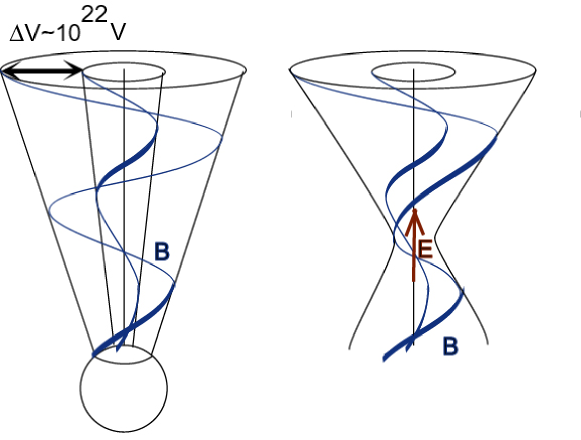
Figure 7: Development of pinching instabilities leads to core contraction, filamentation, disruption of currents and particle acceleration by DC electric field.

The dynamics of the flow near the polar regions is likely to be unstable to magnetic pinching, giving dynamics similar to imploding Z-pinches (e.g.  Rudakov & Sudan, 1997) where explosive X-ray bursts as well as electron and ion acceleration are often observed. In the proposed model the outgoing wave consists of currents strongly concentrated near the axis. Such concentration of poloidal currents is likely to become unstable due to the development of dynamic and resistive instabilities in the strong current region. The fastest growing modes are likely to be pinch, kink and helical modes (see Fig. 7).

At large currents the plasmas in Z-pinches and TOKAMAKs are known to form thin filaments stretching both along and across the direction of the current (Trubnikov, 2002). The typical growth rate of filamentation instabilities is $\sim\omega_{p}v_{d}/c$ where $\omega_{p}$ is the plasma frequency and $v_{d}$ is the drift velocity of the current particles Molvig (1975). Thus, as the current is compressed, at some stage it will break into filaments. Secondary filaments will also be compressed and will undergo further filamentation. The development of instabilities will result in disruption of the current, during which large DC electric fields are created near the O-type point. (The dynamics of current disruption is considered in more detail in Appendix E). This electric field will accelerate run away particles (both electrons, positrons and ions). Thus, the magnetic energy will finally be radiated as electron cyclotron emission and will also be transported away by cosmic rays. The current disruption at each filament will produce a burst of emission, giving a complicated pulse profile for prompt GRB emission.

Initially, the size of the unstable region is of the order of the core radius $r_{D}$ (see Eqns. (30-31)). As the instabilities develop the magnetic energy is dissipated, which leads to a loss of magnetic pressure, so that progressively larger scale modes become unstable (this is similar to an outgoing rarefaction wave). A typical angular size for an unstable current will be of the order of $1/\Gamma$ since in relativistic flows lateral (in $\theta$ direction) forces (e.g., magnetic hoop stresses) are strongly suppressed by a factor $1/\Gamma^{2}$ (e.g.  Bogovalov & Tsinganos, 1999), so that globally (on scales $\theta>1/\Gamma$) the flow cannot adjust to the change of equilibrium on a dynamical time scale – the time scale for establishing an equilibrium in the lateral direction is much larger than the dynamical times scale, by a factor $\sim\Gamma$. The fastest evolution of the flow will take place near the axis, within $\theta\sim 1/\Gamma$, where geometric effects may “beat” the relativistic suppression and produce changes in the field configuration on shorter time scales.

9.3 Shell Emission

The expanding shell will be preceded by a surface (Chapman-Ferraro) current emanating from the poles and flowing to the equator (or vice versa). It will be followed, at a distance of the order of the shell thickness by a reverse current. There are several possible instabilities associated with this configuration. (Since the shell decelerates on average, it is stable to the Kruskal-Schwarzschild instability).

Qualitatively, the interface between two magnetized media is known to be unstable in the case of the Earth’s magnetosphere. Approximately $10\%$ of the incoming energy flux is dissipated at the day side of the magnetosphere (e.g.  Cowley, 1982). In the case of relativistic flows, it is feasible that a similar or even larger fraction of the incoming energy flux may be dissipated. Dissipation may be initiated by several types of instabilities. First, the surface Chapman-Ferraro current becomes unstable due to development of microscopic instabilities on the scales of tens to hundreds of ion Larmor radii (Smolsky & Usov, 1996; Liang et al. , 2003). As a result, the surface current breaks into strongly non-linear fluctuating current and charge layers. These current substructures become strongly dissipative and accelerate particles. Secondly, if the source varies considerably during its activity the surface current may become unstable due to impulsive Kruskal-Schwarzschild instability (see appendix D). The impulsive Kruskal-Schwarzschild instability (IKS) develops if the surface separating magnetic field and matter is accelerated by an electromagnetic pulse. It is similar to Richtmyer-Meshkov instability in fluid dynamics. At the nonlinear stage, IKS instability will lead to formation of small scale structures that will become resistive. During the prompt emission phase, the presence of resistive surface currents may lead to an absorption of a large fraction of the incoming fast mode energy flux. This will result in dissipation of magnetic energy and particle acceleration.

An attractive feature of the shell model is that it predicts $\gamma$-ray emission over large solid angles and few orphan afterglows. The strength of the burst may also depend on the efficiency of radiation generation, which may be a strong function of polar angle, but the kinetic total energy (inferred, e.g. , from early afterglows) should remain approximately constant. Burst viewed from a small angle (as may be inferred from achromatic breaks in the afterglow emission) should be seen to larger distances although a large burst to burst dispersion should be expected. In addition, if emission is confined to a narrow region near the surface of the shell, it will be more variable than in the case of a filled shell, since there is no “radial averaging” over emitters. Simulations of shell emission are also underway which will clarify some of these points.

9.4 Variability

One of the key observational properties that every model of GRBs should address is the short times scales of variability, as short as $\sim 10$ ms. One merit of the electromagnetic model is that it allows the GRB to originate at a much larger radius, up to $\sim 10^{16}$ cm than in the standard, baryonic shock model $\sim 10^{13}$ cm. This stems from the fast that, in an electromagnetically dominated medium, the emission regions (e.g. , large amplitude waves likely to occur in an intermittent turbulence spectrum) may be moving with relativistic velocities in the bulk frame. In this section we consider the statistical properties of radiation emitted by an ensemble of the emitters confined to a narrow spherical shell and subject to relativistic bulk and random motion. We show that relativistic internal motion of ”fundamental emitters” can account for highly intermittent GRB profile with smaller bulk Lorentz factors or larger radii of emission than is usually inferred.

Consider a shell of thickness $\Delta R\ll R$ (in the lab frame) moving relativistically with a bulk Lorentz factor $\Gamma$ (see Fig. 10). Assume that the shell consists of randomly distributed emitters which move randomly with respect to the shell rest frame with a typical Lorentz factor $\gamma_{T}$. If $\theta^{\prime}_{r}$ is the angle (measured in the rest frame of the shell) between the radial direction and emitter’s velocity and $1<\gamma^{\prime}<\gamma_{T}$ is the Lorentz factor of the particle then in the shell frame, emission is beamed into a cone with opening angle $\Delta\theta_{r}^{\prime}\sim 1/\gamma^{\prime}$. In the observer’s frame the emitter’s Lorentz factor is

$$\gamma=\gamma^{\prime}\Gamma\left(1+v^{\prime}V\cos\theta^{\prime}_{r}\right)\sim\gamma^{\prime}\Gamma\left(1+\cos\theta^{\prime}_{r}\right)$$ (112)

where $v^{\prime}=\sqrt{1-1/\gamma^{2}}$ and $V=\sqrt{1-1/\Gamma^{2}}$, and angle between the radial direction and the particle’s velocity in the lab frame is

$$\tan\theta_{r}={v\sin\theta_{r}^{\prime}\over\Gamma(V+v\cos\theta_{r}^{\prime})}\approx{\tan\theta_{r}^{\prime}/2\over\Gamma}$$ (113)

where the approximation assumes $V\sim v\sim 1$. From Eq. (113) it follows that as long as $v\leq V$, the maximum angle with respect to the radial direction that an emitter may have in order to be seen by an observer is $\sim 1/\Gamma$, regardless of the velocity of the emitter. At the same time, the emission cone in the lab frame is $\Delta\theta_{r}\sim 1/\gamma=1/\gamma_{T}\Gamma(1+\cos\theta_{r}^{\prime})$. The addition of internal relativistic motion makes the emission beams much narrower but the visible emitting volume increases only by a factor of 4, when compared with cold emitters. For relativistic internal motion, the number of emitters seen at a given time will decrease as $1/\gamma_{T}^{2}$. At the same time the flux from each emitter will increase as $\gamma_{T}^{4}$ (Two factors of $\gamma_{T}$ coming from the fact that all the emission is confined within a narrow beam $1/\gamma_{T}^{2}$ and two factors of $\gamma_{T}$ coming from the relativistic contraction of a pulse). Thus, the “thermal”’ spread in the motion of emitters can drastically change the estimates of the Lorentz factors. The Lorentz factor inferred from variability is, in fact, a product of the bulk and “thermal” Lorentz factors. Since for a given $\Gamma$ the number of emitters seen at a given time decreases $\propto 1/\gamma_{T}^{2}$, modest values $\gamma_{T}\leq\Gamma$ suffice to produce large variations.

9.5 Causal structure of electromagnetic outflows

Electromagnetic outflows have a different casual structure from hydrodynamic flows. Initial evolution of both types of flow is similar: close to the central source both electromagnetic and hydrodynamic flows are subsonic and fully causally connected. Later, after breakout, both types of flows are linearly accelerated by magnetic and/or pressure forces $\Gamma\sim r$. Hydrodynamic flows become causally disconnected after passing through a sonic point where $\Gamma=\sqrt{3/2}$. An electromagnetic flow can pass through the fast magnetosonic point provided that initially $\sigma_{0}>\Gamma^{2}$, and will become causally disconnected over small polar angles $\Delta\theta\sim 1/\Gamma$.

After the photosphere, when magnetization parameter $\sigma$ increases by many orders of magnitude, causal behavior of the types of flow is drastically different. Hydrodynamic flows virtually do not establish a causal contact over angles large than $1/\Gamma$. Contrary to that, electromagnetically-dominated flows quickly re-establish causal contact. Lyutikov et al. (2003) showed that sub-Alfvenic ejecta re-establishes a causal contact over the visible patch of $1/\Gamma$ in just one dynamical time scale (after doubling in radius). In fact, causal contact may be established over whole expanding shell after a time $t_{\rm c}\sim t_{s}\Gamma^{2}$. At this point the shell is fully causally-connected .

Causal contact over large angles of the shell is established by waves propagating almost backward in the shell frame. Here lies a principal difference between strongly magnetized flows on the one hand and weakly and non-magnetized flows on the other. Strongly magnetized flows can be subsonic with respect to the velocity of the signals in the flow, while weakly magnetized flows are always supersonic. Thus, in case of weakly magnetized flows waves emitted backward in the shell frame are ”advected” with the flow and cannot reach to large angles. Strongly magnetized flows are subsonic, so that waves can outrun the flow and reach to large angles. In doing so they leave the shell (which has a thickness either $ct_{s}$ or $R/\Gamma^{2}$), but this does not present a problem since the fast magnetosonic waves become light waves if they propagate into a low density medium.

The causal structure of electromagnetic shells plays an important role in maintaining the coherence of large scale magnetic fields. If a surface of relativistically expanding magnetized shell is perturbed at some radius, it can quickly propagate information (e.g. magnetic pressure) over the visible angle $1/\Gamma$, so that the shell can have quasi-homogeneous properties despite possible inhomogeneities in the circumstellar medium and in ejecta. In hydrodynamic, $\sigma\ll 1$, or hydromagnetic, $\sigma\sim 1$ (e.g.  Spruit et al. , 2000), models only under strict homogeneity of the surrounding medium and of the ejecta will the two causally disconnected parts of the flow have similar properties.

Thus, the electromagnetic model provides a solution to the puzzle of how to launch a blast wave that extends over an angular scale $>>\Gamma^{-1}$ and where the individual parts are out of causal contact. In the electromagnetic model, the energy is transferred to the blast wave by a magnetic shell which is causally connected at the end of the coasting phase.

10 Afterglows

As the magnetic shell expands, its energy is gradually transfered to the preceding forward shock wave. In a constant density medium this transfer occurs at the end of the coasting phase. At later times, most of the energy released by the central, spinning, magnetic rotator is carried by the shocked interstellar medium. The structure of the blast wave is well approximated by the self-similar adiabatic solution (Blandford & McKee, 1976, 1977), but with angle-dependent expansion. If the total energy released per unit solid angle is $E_{\Omega}\sim L_{\Omega}t_{s}$, then (Blandford & McKee, 1976)

$$\Gamma\sim\left({17E_{\Omega}\over 2\rho_{ex}c^{5}t^{3}}\right)^{1/2}$$ (114)

If, in addition, the energy release is as argued above (see Eq. (110)), then

$$\Gamma\sim\left({17E_{0}\over 2\rho_{ex}c^{5}}\right)^{1/2}{t^{-3/2}\over\sqrt{\theta^{2}+\theta_{0}^{2}}}\approx{\Gamma_{0}(t)\over\theta}\mbox{ for $\theta\gg\theta_{0}$.}$$ (115)

As long as the blast wave remains relativistic the energy in the magnetic shell decreases slowly (logarithmically), so that the relativistic blast wave stage is coexistent with the self-similar stage of the magnetic shell as long as the shock remains relativistic, $r<r_{{\rm NR}}\equiv(E_{\Omega}/\rho c^{2})^{1/3}\sim 10^{18}$ cm. The afterglow phase usually becomes unobservably faint after the expansion speed becomes mildly relativistic. At that point the forward shock finally detaches from the magnetic shell and will expand non-relativistically and become more spherical with time, resembling a normal supernova remnant.

Relativistic particles are accelerated in the blast wave producing the observed afterglow in a manner which is essentially similar to what is proposed for fluid models. There are, however, some differences. First, the contact discontinuity itself may be an important source of magnetic flux through IKS instability (appendix D). Then the afterglow may result from a mixture of relativistic particles, derived from the shock front with magnetic field derived from the shell, much like what seems to happen in regular supernova remnants.

The development of the IKS instability will lead to distortion of the CD. The perturbations propagate mostly orthogonally to the magnetic field. In the linear regime, this will lead to ”braiding” of the field lines, so that large scale ordered field remains mostly unaffected. In the nonlinear regime a degree of ordering of the magnetic field may be preserved as well. Later, at the afterglow phase, the IKS instability will lead to mixing of the ejecta with circumstellar material. This requires that the source remains active for much longer than 100 sec. There are indications, e.g. in case of GRB030329, that this indeed may be the case. Since during the development of the IKS instability field lines will mostly braid keeping large scale field ordered, an ordered component of the field will be introduced to the shocked circumstellar material and may explain the polarization of afterglows.

In addition to dynamic instabilities, the CD may also be unstable to resistive instabilities like the tearing mode. The magnetic field from the shocked circumstellar material piles up on the CD, so that however small the field is in the the bulk of the flow, it plays an important part in a thin boundary layer near the CD (Lyutikov, 2002a). Thus the CD becomes a rotational discontinuity and should be susceptible to resistive instabilities, similar to the case of Earth magnetopause (Galeev et al. , 1986). The growth of tearing mode occurs on wave modes propagating orthogonally to the magnetic field. As a result “percolated” magnetic filaments form that connect outside and inside plasma.

The second difference in the afterglow dynamics between the electromagnetic l and fireball models is that the form of the forward shock is a definite function, determined by the current distribution in the shell. This is also the principal difference between relativistic and non-relativistic (Sedov) blast waves. In the non-relativistic case explosion quickly “forgets” the details of the central source and dynamics is determined only by the total energy release, while in the strongly relativistic regime the forward shock also carries information about the angular energy distribution of the source. The form of the blast wave would reflect both the form of the driver (magnetic shell) and subsequent evolution of the shock (Kompaneets, 1960; Shapiro, 1979; Granot et al. , 2003). In the strongly relativistic regime, the form of the forward shock is mostly determined by the form of the electromagnetic driver, so that the motion of the shock is mostly ballistic (Shapiro, 1979), with little sideways expansion (so the in the rest frame $v_{\theta}^{\prime}\ll c$, not $\sim c/\sqrt{3}$ as is commonly assumed); this is confirmed by recent semi-analytical (Granot et al. , 2003) and fully relativistic hydrodynamic calculations Cannizzo et al.  (2003).

Thus, there is little lateral evolution between the forward shock and the contact discontinuity. If we continue to use our simple model, we find that the afterglow expansion varies most rapidly and remains relativistic for longer times closer to the symmetry axis. In particular, if the outgoing waves correspond to the outflow carrying axial current (section 8) the energy carried by the forward shock wave will scale as $E_{\Omega}\sim 1/\sin^{2}\theta$ and the Lorentz factor of the forward shock $\Gamma_{s}\sim\Gamma_{0}/\sin\theta$. (Note that at the afterglow stage the Lorentz factor of the forward shock depends only on the energy that the source released per unit solid angle $E_{\Omega}$ and different from the Lorentz factor of the CD $\Gamma_{CD}$). This type of shock has been named “structured jet” (or universal jet) (Rossi et al. , 2002a), though in our model there is no proper “jet”, but simply a non-spherical outflow. As $E_{\Omega}\propto\sin^{-2}\theta$ the energy contained in each octave of $\theta$ is roughly constant, so that the inferred explosion energy with our simple model will be roughly independent of $\theta$ and characteristic of the total energy. This, combined with the assumption that the total energy of GRBs is related to kinetic energy of a critically rotating relativistic stellar object, explains a narrow range of inferred GRB energies (Frail et al. , 2001). Most importantly, the resulting non-spherical blast wave emits in all directions. However, the intensity of this emission is strongest along the poles. This means that the most intense bursts and afterglows in a flux-limited sample will be seen pole-on and can exhibit achromatic breaks when $\Gamma\sim\theta^{-1}$, which might be mistaken for jets. The observational appearance of such “structured jets” have been investigates by several collaborations (Rossi et al. , 2002a; Granot et al. , 2003; Perna et al. , 2003). The overall conclusion is that “structured jets” provide the best fit to afterglow emission properties (Granot et al. , 2003) and reproduce well luminosity function of GRBs (Perna et al. , 2003) including a possibility of unified description of GRBs and X-ray flashes (the only X-ray flashes with measured redshift had a total energy comparable to classical GRBs (Soderberg et al. , 2003)).

In conclusion, we argue that observational appearance of GRB afterglows depends mostly on two parameters: (i) explosion energy (more precisely, on the ratio on the explosion energy to circumstellar density) and, most importantly, (ii) the viewing angle that the progenitor’s axis is making with the line of sight. This possibility, that all GRBs are virtually the same but viewed at different angles resembles unification scheme of AGNs.

11 Observational implications

Prompt and afterglow polarization. Recent observations by the RHESSI  satellite have been interpreted as evidence for large polarization of the prompt $\gamma$-ray emission of GRBs (Coburn & Boggs, 2003). This has bee contested by (Rutledge & Fox, 2003). If the large polarization is confirmed, it could be most naturally explained as a synchrotron radiation from a large scale magnetic field. In order to produce very high polarization the coherence scale of the field should be larger than the size of the visible emitting region. This can be achieved naturally achieved if the flow is magnetically-dominated (Lyutikov et al. , 2003).

Several natural correlations between the prompt GRB polarization and other parameters follow from the model and can be tested with future observations. The maximum amount of polarization in our model is related to the spectrum of emitting particles, being higher for softer spectra (Lyutikov et al. , 2003). This points to a possible correlation between the amount of polarization and hardness of the spectrum.

Large scale field structure in the ejecta emission may also be related to polarization of afterglows if fields from the magnetic shell are mixed in with the shocked circumstellar material. The fact that the magnetized boundary becomes “leaky” and both plasma and magnetic field are transported across it has been amply demonstrated by decades of space experiments (e.g.  Cowley, 1982). The transport occurs either due to microscopic resistive instabilities of the surface current (similar to the so called flux transfer events at the day side of Earth magnetosphere and instabilities at the heliopause (Fahr et al. , 1986)) or due to dynamic (e.g. RT) instabilities. In the case of Earth and Solar heliopause approximately $10\%$ of the incoming plasma is transfered through the CD. In case of GRB the CD may also be unstable due to dynamical impulsive Kruskal-Schwarzschild instability (appendix D). Since both resistive (e.g. tearing mode) and dynamics instabilities are expected to develop mostly on the waves propagating orthogonally to the large scale magnetic field, a degree of field ordering will be preserved. As a result, a comparably large fractional polarization may be observed in afterglows as well. In this case, since the preferred direction of polarization is always aligned with the flow axis, the position angle should not change through the afterglow (if polarization is observed both in prompt and afterglow emission the position angle should be the same). Also, polarization should be most independent of the ”jet break” moment. This is in a stark contrast with the jet model, in which polarization is seen only near the ”jet break” times and the position angle is predicted to experience a flip during the ”jet break” (Ghisellini & Lazzati, 1999; Sari, 1999) . Current polarization data are not completely decisive. In most cases the position angle remains constant (Gorosabel et al.  2003; Covino et al. 2003a, b; Barth et al.  2003; Bersier et al.  2003), while the amount of polarization does not show any correlation with the ”jet break”. This is consistent with the presence of large scale ordered magnetic fields in the afterglows. But there are also exceptions Rol et al.  2003; Greiner et al.  2003, when the position angle does show some variations. (A model of Rossi et al.  (2002a) of structured jets also predicts constant position angle, but since no large scale magnetic field is assumed the polarization features are still related to the jet break times).

Structured jet. As discussed in Section 10 our model gives a theoretical foundation for the “structured jet” profile of the external shock. We would like to stress once again that there is no proper jet in our model, but a non-spherical outflow, so that a break in the light curve is seen when $\Gamma\theta_{ob}\sim 1$.

XRF flashes. Another testable prediction of the model is that we should observe much more numerous X-ray flashes (XRFs), which may be coming “from the sides” of the expanding shell where the flow is less energetic and the Lorentz boosting is weaker. In addition, the total bolometric energy inferred for XRFs (presumably from observations of early afterglows before radiative losses become important) should be comparable to the total bolometric energy of $\gamma$-ray bursts. (The total X-ray fluences may be quite different since this would include a correction for the unknown radiative efficiency as a function of the polar angle). At present, a single X-ray flash with measured redshift suggests had an energy similar to those associated with GRBs (Soderberg et al. , 2003). Generally, the distributions of parameters of XRFs should continuously match those of GRBs.

Short-long dichotomy. Our model can also explain a short versus long dichotomy in GRBs. We associate short bursts with the instabilities of polar currents while long with instabilities of shell currents. Our analytical solutions for electromagnetic fields diverge on the axis; in reality the axial current density will have finite angular width. If an observer is located within this small angle he would see a burst that would be shorter since the Lorentz factors of the outflow are higher closer to the axis.

Hard-soft evolution and $E_{peak}-\sqrt{L}$ correlation. Magnetically-dominated flows may also explain the observed correlations between various GRB parameters, though the lack of a testable particle acceleration model makes the arguments below only suggestive. For example the trend of GRB spectra to evolve from hard to soft during a pulse is explained as a synchrotron radiation in an expanding flow with magnetic field decreasing with radius $B\propto\sqrt{L}/r$ (later in a pulse emission is produced further out where magnetic field is weaker, so that the peak energy will be lower; this is similar to ”radius-to-frequency mapping” in radio pulsars and AGNs). A correlation between peak energy and total luminosity, $E_{peak}\sim\sqrt{L}$ (Lloyd-Ronning & Ramirez-Ruiz, 2002) follows from the assumption of a fixed typical emission radii and fixed minimum particle energy. Both of these correlations are independent of the bulk Lorentz factor, but depend on the lower energy cut-off in the spectrum of accelerated particles.

No reverse shock. Another consequence of the model is that no emission from the reverse shocks is expected in electromagnetic models. When plasma magnetization becomes of the order of unity relativistic MHD shock conditions are modified: shocks becomes less dissipative; in the force-free limit shocks cannot exist at all. Early optical flashes, which are conventionally associated with reverse shock (e.g.  Mészáros & Rees, 1997; Kobayashi & Zhang, 2003; Kumar & Panaitescu, 2003), should have a different origin. A possible explanation is the formation of a radiative precursor that pre-accelerates the medium, loads it with e+- pairs and produces soft emission (Beloborodov, 2002; Thompson & Madau, 2000)

12 Discussion

In this paper we have explored the “electromagnetic hypothesis” for ultra-relativistic outflows, namely that they are essentially electromagnetic phenomena which are driven by the energy released by spinning black holes or neutron stars and that this electromagnetic behavior continues into the source region even when the flows become non-relativistic. In this model the energy to power the GRBs comes eventually from the rotational energy of the progenitor. It is first converted into magnetic energy by the dynamo action of the unipolar inductor, propagated in the form of Poynting flux-dominated flow and then dissipated at large distances from the sources. We have taken an extreme view that the flows become essentially force-free and explored the consequences of this assumption. Real GRB outflows must contain both baryonic matter and approach near-equipartition in the emission regions.

This model envisions GRB outflows as an electric circuit in which the central source acts as a power-supply generating a very simple current flow – along the axis, the surface of the shell and the equator. In practice, it is the detailed electrodynamics in the vicinity of the outgoing light surface that fixes the poloidal magnetic field and electrical current distributions. We can therefore change these (still, of course, maintaining the force-free condition) and solve for a new evolution of the magnetic shell and blast wave. A broader distribution of currents will generally produce a less pronounced expansion along the axis and change somewhat the statistics of the observed afterglows. Alternatively, the central source can collimate the flows to even more narrow (cylindrical) expansion. In the solution above, we ignored the poloidal magnetic field and, consequently, the angular momentum. These can be reinstated perturbatively into the solution. Their influence wanes with increasing radius. Other ways to obtain different solutions include changing the temporal variation of the source from the one satisfying self-similar expansion to a more general variation. As the individual parts of the blast wave expand essentially independently, when ultra-relativistic, there are no new issues of principle to address in solving these problems. When the blast wave becomes non-relativistic the interior gas will be roughly isobaric and the shell will become more spherical with time.

The most striking implications of the electromagnetic hypothesis are that particle acceleration in the sources is due to electromagnetic turbulence rather than shocks and that the outflows are cold, electromagnetically dominated flows, with very few baryons at least until they become strongly dissipative. The major drawback of the current model is the lack of the detail model of energy dissipation and particle acceleration in relativistic magnetically-dominated medium. This is a difficult problem. The problem with magnetic dissipation may be exemplified by the better studied way of dissipation of magnetic energy, through reconnection. Reconnection physics is highly uncertain: it depends crucially on the kinetic and geometric properties of the plasma, which is very hard to test observationally. Often, various instabilities (based on inertial or cyclotron effects, on ions or electrons) often seem to account equally well (with astrophysical accuracy) for the observed phenomena. This is an important uncertainty since the principle scale of the reconnection region (related, for example, to electron or ion skin depth, Larmor radius or magnetic Debye radius) is crucial in determining the rate of reconnection (e.g.  Birk et al. , 2000). This situation may be contrasted with the shock acceleration schemes, where a qualitatively correct result for the spectrum of accelerated particles can be obtained from simple macroscopic considerations.

An important implication of the electromagnetic model is that supernova explosions may be magnetically driven as well (Leblanc & Wilson, 1971; Bisnovatyi-Kogan, 1971). A number of research groups are investigating this possibility, mostly through numerical modelling (Mizuno et al. , 2003; Proga et al. , 2003).

Another uncertainty in the model is how baryon-free the flow can become. At early stages large fluxes of low energy neutrinos are expected. They will drive the material up the field lines into the magnetosphere, while gravity will try to pull the matter back into the disk. We require that the resulting outflow be extremely clear of baryons ($\sim 10^{-9}$ in energy flux); numerical simulations are required to see if this is possible (e.g.  Thompson et al. , 2001).

If GRBs are electromagnetically-driven they should not be associated with strong, high energy neutrino sources. A gravitational wave signal is expected in some, though not all, source models and would be strongly diagnostic if ever detected.

Electromagnetic models are also consistent with being possible sites of UHECR acceleration (Vietri, 1995; Waxman, 1995; Milgrom & Usov, 1995; Wick et al. , 2003) if the corresponding energy balance of UHECR and GRBs agree (Waxman, 2002; Vietri et al. , 2003) and if assuming that the GZK cut-off is indeed observed in the spectrum of UHECRs (Bahcall & Waxman, 2002). Primarily, the total available electric potential in GRBs, $\sim 10^{22}$ V, is sufficient for acceleration of UHECRs. UHECR energies are mostly likely radiation-limited and not acceleration-limited, but, at late stages of GRB expansion, synchrotron losses become sufficiently small.

In addition to Fermi acceleration at the forward shock, electromagnetically-dominated flows provide several possible acceleration schemes in their own right. (Note that, in order to explain UHECRs, shock acceleration models have to assume that turbulent EMF reaches approximate equipartition behind relativistic shocks (e.g.  Dermer & Humi, 2001); this requirement makes these models akin to electromagnetic models.) There is a large inductive electric field $E_{\theta}$ which creates a large potential difference (4) between the polar and equatorial flux surfaces. Thus, in order for a particle to gain the total energy it should traverse from pole to equator (or a considerable part of this path). This should be done on expansion time scale in order to avoid adiabatic loss; this is possible at the end of the relativistic stage. (Note that, at late stages, most of the energy is in the forward shock the total pole-to-equator electric potential drop remains approximately constant as long as the expansion is relativistic and starts to decrease only at the non-relativistic stage.) This crossing of the potential surfaces may be done either kinetically, e.g. due to a drift, or resistively, e.g. at O-type point (e.g.  Trubnikov, 2002; Vasyliunas, 1980).

In this paper we have discussed the basic principles that may be important in electromagnetically-dominated outflows. At the present stage the model is definitely less developed than the hydrodynamics fireball model and a lot needs to be done to vindicate it, but the possible fundamental advantages of electromagnetic models outlined here make it, in our opinion, a very promising approach. From a more theoretical perspective, there is much to be learned about the properties of force-free electromagnetic fields, especially their dissipation. The possible relationship of the GRB fluctuation power spectrum to an underlying turbulence spectrum is especially tantalizing. Undoubtedly, numerical simulations will be crucial as the problem is essentially three-dimensional. Force-free electromagnetism is easier to study than relativistic MHD and may well be a very good approximation in many of these sources.

If, as we have argued, magnetic fields do play an important dynamical role in GRBs, there is the between supersonic MHD outflows $\sigma\leq\Gamma^{2}$ (e.g.  Vlahakis & Königl, 2003a; Fendt & Ouyed, 2003) and the subsonic force-free model, $\sigma\geq\Gamma^{2}$, considered in this paper. As we have discussed these two alternatives have very different properties coming from different causal structures of the flow. Observationally, it will be hard to distinguish between the two since even in the strongly magnetized case we expect that in the emission region the fields approach equipartition (since then plasma emits most efficiently).

Finally, we give a concise list of the observational properties of the GRBs which are explained or foreseen in the electromagnetic model. GRBs properties should most depend on the observer angle with respect to the jet axis. Electromagnetic model produces “structured jet” with energy $E_{\Omega}\propto\sin^{-2}\theta$; there is no problem with “orphan afterglow” since GRBs are produced over large solid angle; X-ray flashes are interpreted as GRBs seen “from the side”, but their total energetics should be comparable to proper GRBs; overall energy of GRBs is expected to have a small scatter if it is related to a critically rotating relativistic object; the model can qualitatively reproduce hard-to-soft spectral evolution as a synchrotron emission in ever decreasing magnetic field $B\propto\sqrt{L}/r$ ($L$ is luminosity, $r$ is emission radius), akin to ”radius-to-frequency mapping” in radio pulsars and AGNs; similarly, the correlation $E_{peak}\sim\sqrt{L}$ is also a natural consequence. Finally, high polarization of prompt emission may also be produced: it should correlate with the spectral index; mixing between circumstellar material and ejecta will result in the same position angles of the prompt emission and afterglow which should be constant over time; fractional polarization should be mostly independent of the “jet break” time, but may show variations due to turbulent mixing.

13 Application to other sources

Many of the principles described in this work may be applied to other astrophysical sources like pulsars, (micro)quasars and AGNs (Blandford, 2002). Despite the apparent differences (inner boundary condition for neutron stars and black holes, time (non-)stationarity, optical thickness) it is plausible that all these sources produce ultra-relativistic magnetically-dominated outflows with low baryon density. Energy, transported primarily by magnetic fields, is dissipated far away from the source due to the development of MHD current instabilities. Particles are accelerated in localized current sheets by DC electric fields and/or electromagnetic turbulence producing bright knots (in AGNs) and a variety of bright spots in pulsar jet, best observed in the Crab. In situ acceleration is required in both AGNs and pulsars since the life-time of emitting particles is shorter than the dynamical time. Qualitatively, magnetically-dominated jets are expected to be more stable than their fluid counterparts (Beskin & Pariev, 1993). In the case of AGN, recent observation of TeV emission from blazers with a very short time scale variability (Krennrich et al. , 2002) favors magnetically-dominated jets (e.g.  Lyutikov, 2002b) since the two leading models of jet composition - leptonic and ionic - both have difficulties in explaining the fast variability (problem for ion-dominated jets, since cyclotron times are very long for ions) and total energy content (since leptons suffer strong radiative losses at the source due to radiation drag). The flow evolution in all these systems may proceed in a similar wave. Jets are launched in the vicinity of a central object (a BH-disk system or a neutron star) where the flow is subsonic and in a dynamical balance. As the flow propagates out jets become laterally imbalanced, just as with GRBs, the lateral dynamics is suppressed by relativistic kinematics, so that the jet cannot adjust to the change of equilibrium on dynamical time scale. After a jet has propagated $\Gamma^{2}$ dynamical times, the lateral dynamics starts to become important. A particularly strong evolution will take place in the core of the jet, where magnetic hoop stresses may lead to the collapse of the flow toward the axis. For example, AGN jets may originate close to the central black hole with a Schwarzschild radius $r_{s}\sim 10^{13}$ cm with a typical Lorentz factor $\Gamma\sim 10-30$. Then the dynamical evolution and the onset of emission occurs on a scale $\sim\Gamma^{2}r_{s}\sim 10^{15}-10^{16}$ cm. In pulsars acceleration occurs on a scale of light cylinder, $r_{s}\sim 10^{10}$ cm,with a Lorentz factor $\Gamma\sim 100-1000$, then the dynamical instabilities occur at $\sim 10^{14}-10^{16}$ cm.

Appendix A Dynamics of magnetized pair-loaded flows (minifireballs)

In this appendix we consider the far field dynamics of a spherically symmetric magnetized wind. The dynamics of such warm magnetized wind is controlled by three parameters: energy $L$, mass flux $\dot{M}$ and the electro-motive force ${\cal E}$ produced by the central source. The central source loses energy in two forms: mechanical $L_{M}$ and electromagnetic $L_{EM}$ luminosities.

$$L=L_{M}+L_{EM}$$ (A1)

We wish to understand how the parameters of a fully relativistic flow (velocity $\beta$, pressure $p$, magnetization $\sigma$) evolve for an arbitrary ratio of both $L_{EM}/L_{M}$ and $p/\rho$ ($\rho$ is the rest-frame mass density).

The asymptotic evolution of the flow is determined by conserved quantities which may be chosen as the total luminosity $L$, the mass flux $\dot{M}$ and the EMF ${\cal E}$. Thus, the central source works both as thruster and as a dynamo. We follow the flow evolution starting from some small inner radius where we assume that a flow with given $L,\,\dot{M}$ and ${\cal E}$ (in a form of toroidal magnetic field) is generated. Thus, we avoid the important question of how the flow is launched. Another important assumption that we make is that the expansion is radial.

The formal treatment of the problem starts with the set of RMHD equations which can be written in terms of conservation laws (50) in which we assume that fluid is polytropic with adiabatic index $\Gamma_{a}$: $w=\rho+{\Gamma_{a}\over\Gamma_{a}-1}p$. (We assume that the adiabatic index $\Gamma_{a}$ is constant for algebraic simplicity.)

Writing out eqns. (50) in coordinate form and assuming a stationary, radial, spherically symmetric outflow with toroidal magnetic field, we find

$${1\over r^{2}}\partial_{r}\left[r^{2}(w+b^{2})\beta\Gamma^{2}\right]=0$$ (A2)

$${1\over r^{2}}\partial_{r}\left[r^{2}\left((w+b^{2})\beta^{2}\Gamma^{2}+(p+b^{2}/2)\right)\right]-{2p\over r}=0$$ (A3)

$${1\over r}\partial_{r}\left[rb\beta\Gamma\right]=0$$ (A4)

$${1\over r^{2}}\partial_{r}\left[r^{2}\rho\beta\Gamma\right]=0$$ (A5)

The above relations can be simplified if by defining

$$L=4\pi r^{2}\beta\,{\Gamma}^{2}\,\left(b^{2}+{\Gamma_{a}\over\Gamma_{a}-1}\,p+\rho\right),\,\,\,\dot{M}=4\pi r^{2}\beta\,\Gamma\,\rho,\,\,\,{\cal E}=2\sqrt{\pi}r\,\beta\,\Gamma\,b$$ (A6)

where ${\cal E}$ is the electromotive force.

It is convenient to introduce two other parameters: the magnetization parameter $\sigma$ as the ratio of the rest-frame magnetic and particle energy-density and a fast magnetosonic wave phase velocity $\beta_{f}$

$$\sigma={b^{2}\over w}={{\cal E}^{2}\over L\beta-{\cal E}^{2}},\,\,\,\beta_{f}^{2}={\sigma\over 1+\sigma}+{\Gamma_{a}p\over(1+\sigma)w}=\left(\Gamma_{a}-1\right)\left(1-{\Gamma\dot{M}\over L}\right)+(2-\Gamma_{a}){{\cal E}^{2}\over L\beta}$$ (A7)

Using the three conserved quantities $L,\,\dot{M}$ and ${\cal E}$ the evolution equation becomes

$${1\over 2\beta^{2}\Gamma}\partial_{r}\Gamma={(\Gamma_{a}-1)\left(\beta L-\beta\Gamma\dot{M}-{\cal E}^{2}\right)\over r\,\left(\beta L(\beta^{2}+1-\Gamma_{a})+(\Gamma_{a}-1)\beta\Gamma\dot{M}-(2-\Gamma_{a}){\cal E}^{2}\right)}$$ (A8)

Eliminating ${\cal E}$ in favor of $\Gamma_{f}$ we get a particularly transparent form for the evolution of Lorentz factor

$${\left({\Gamma}^{2}-{{{\Gamma}_{f}}}^{2}\right)\over\beta^{2}\Gamma^{3}}\partial_{r}\Gamma={2p\Gamma_{a}\over(w-\Gamma_{a}p)r}$$ (A9)

Equation (A9) is nozzle-type flow (e.g. (Landau & Lifshits, 1975a)); in astrophysical context it is best known for Parker’s solutions of the solar wind (Parker, 1960). The lhs of eq. (A9) contains a familiar critical point at the sonic transition $\Gamma=\Gamma_{f}$. The positively defined first term on the rhs describes the evolution of Lorentz factors due to pressure effects. In the case of purely radial expansion the magnetic gradient forces are exactly balanced by the hoop stresses, so that magnetic field does not contribute to acceleration. From Eq. (A9) it follows that super-fast-magnetosonic flows accelerate while sub-fast-magnetosonic flows decelerate. It also it follows that terminal Lorentz factor of the flow is determined by the condition $\partial_{r}\Gamma=0$ which implies that either $p=0$ or $\beta=0$. Condition $\beta_{\infty}=0$ can be reached only for subsonic flows with ${\cal E}=0$; (a steady state perfect MHD radial magnetized flow with ${\cal E}\neq 0$ cannot slowdown to a halt at infinity). Neglecting the $\beta_{\infty}=0$ solution, the terminal velocity of magnetized flow is determined only by the condition $p=0$:

$$L=\Gamma_{\infty}\dot{M}+{{\cal E}^{2}\over\beta_{\infty}}$$ (A10)

For each set of parameters ($L$, $\dot{M}$ and ${\cal E}$) there are generally two solutions for the terminal four-velocity corresponding to the supersonic and subsonic solutions. Th only exception is the unmagnetized branch, ${\cal E}_{0}$. In the absence of magnetization the terminal (supersonic) Lorentz factor is uniquely determined by $\Gamma_{\infty}=L/\dot{M}$. In GRB applications we are mostly interested in the supersonic solutions (the subsonic solutions are important for pulsar winds, (e.g.  Kennel & Coroniti, 1984)).

For supersonic solutions, the unmagnetized branch with ${\cal E}_{0}$ is qualitatively different from magnetized branch. In the absence of magnetization, the terminal (supersonic) Lorentz factor is determined by $\Gamma_{\infty}=L/\dot{M}$ (in the subsonic regime $\beta\sim r^{-2}$ and $p,\,\rho=$ const as with the breeze solution of the solar wind). For finite magnetization there are two solution: a larger one corresponding to super-fast-magnetosonic flow and a smaller one corresponding to a sub-fast-magnetosonic flow. In particular, for large $L/\dot{M}\gg 1$ the supersonic terminal proper velocity reaches

$$\Gamma_{\infty}\beta_{\infty}\sim{L-{\cal E}^{2}\over\dot{M}}$$ (A11)

Thus, for a given ratio $L/\dot{M}$ the terminal Lorentz factor decreases with increasing ${\cal E}$ - magnetic field provides an effective inertial loading of the flow.

For non-zero magnetization the terminal velocity cannot be determined uniquely from a given $\dot{M}$ and ${\cal E}$ - this problem is the results of our neglect of details of acceleration (Michel, 1969; Goldreich & Julian, 1970). Yet, there is a trick, initially suggested by (Michel, 1969), which allows one to select from a family of solutions a ”minimum torque” solution (in the terminology of Michel (1969)). A more careful examination (Goldreich & Julian, 1970; Kennel et al. , 1983) proves that indeed, for strongly magnetized flows, when the pressure contribution to acceleration is not important, the minimum torque solution is the correct one.

In case of non-zero magnetization, for a given ratio ${\cal E}$ solutions exist only for $L/\dot{M}$ larger than some critical value $L/\dot{M}=(1-({\cal E}^{2}/L)^{2/3})^{-3/2}$, corresponding to $\beta_{\infty}=({\cal E}^{2}/L)^{1/3}$ (alternatively, $\beta_{\infty}=1/\sqrt{1+(\dot{M}/{\cal E}^{2})^{2/3}}$, reached at ${\cal E}^{2}\left(1+(\dot{M}/{\cal E}^{2})^{2/3}\right)^{3/2}$). This is the Michel solution, which we can reformulate now stating that for fixed $\dot{M}$ and ${\cal E}$ the minimum energy loss is reached at $\beta_{min}$. It is expected that, as the flow become stronger magnetized, its terminal evolution asymptotes to the Michel solution.

The above relations may be expressed in term of terminal magnetization parameter $\sigma_{\infty}$ and the terminal velocity of the supersonic wind

$$\Gamma_{\infty}={L\over\dot{M}_{0}(1+\sigma_{\infty})},,\,\,\,\sigma_{\infty}={{\cal E}^{2}\over\Gamma_{\infty}\beta_{\infty}\dot{M}_{0}}.$$ (A12)

Assumption $\beta_{\infty}=\beta_{min}$, then gives

$$\left(1+(\beta_{\infty}\Gamma_{\infty}\sigma_{\infty})^{2/3}\right)^{3/2}={\Gamma_{\infty}\sigma_{\infty}\over\beta_{\infty}^{2}}$$ (A13)

which in the strongly relativistic limit gives the Michel solution

$$\Gamma_{\infty}=\sqrt{\sigma_{\infty}}$$ (A14)

We can also relate the terminal magnetization $\sigma_{\infty}$ to the magnetization at the source - more specifically to magnetization at the sonic point $\sigma_{f}$. Using (A12) we find that at any point in the flow the magnetization parameter is given by

$$\sigma={\beta_{\infty}\sigma_{\infty}\over\beta(1+\sigma_{\infty})-\beta_{\infty}\sigma_{\infty}}$$ (A15)

To relate the magnetization at infinity to the magnetization at the sonic point we need solve for the velocity at the sonic point $\beta_{f}$. Using (A7) and (A15) we find an equation for $\beta_{f}$

$$\beta_{f}^{2}=(\Gamma_{a}-1)\left(1-{\Gamma_{f}\over\Gamma_{\infty}(1+\sigma_{\infty})}\right)+(2-\Gamma_{a}){\sigma_{\infty}\over 1+\sigma_{\infty}}{\beta_{\infty}\over\beta_{f}}$$ (A16)

In the absence of mass flux, $\dot{M}=0$, $\Gamma_{\infty}=\infty$,

$$\beta_{f}=\left\{\begin{array}[]{ll}\sqrt{\Gamma_{a}-1}+{(2-\Gamma_{a})\sigma_{\infty}\over 2(\Gamma_{a}-1)}&\mbox{ if $\sigma_{\infty}\ll 1$}\\ 1-{2-\Gamma_{a}\over(4-\Gamma_{a})\sigma_{\infty}}&\mbox{ if $\sigma_{\infty}\gg 1$}\end{array}\right.$$ (A17)

Thus, for strongly magnetized flow, $\sigma_{\infty}\gg 1$, $\Gamma_{f}=\sqrt{2\sigma_{\infty}}$ for $\Gamma_{a}=4/3$. Using above expressions for the sonic velocity we find a relationship between the magnetization at the sonic point and infinity (for supersonic flows):

$$\sigma_{f}=\left\{\begin{array}[]{ll}{\sigma_{\infty}\over\Gamma_{a}-1}&\mbox{ if $\sigma_{\infty}\ll 1$}\\ {(4-\Gamma_{a})\sigma_{\infty}\over 2}&\mbox{ if $\sigma_{\infty}\gg 1$}\end{array}\right.$$ (A18)

Thus, we always have $\sigma_{\infty}<\sigma_{f}$, but they remain of the same order of magnitude: the magnetization of the flow changes only slightly as the flow propagates away from the launching point to infinity. The reason for constant $\sigma$ in the supersonic regime is that both in the case $p\gg\rho$ (linear acceleration stage) and $p\ll\rho$ both the plasma and the magnetic field energy densities in the flow change with the same radial dependence ($\sim r^{-4}$ and $\sim r^{-2}$ correspondingly).

Generally there are two branches of solutions: supersonic and subsonic. In the limit $\Gamma_{\infty}\rightarrow\infty$ (this is equivalent to neglecting the mass loss rate of the central source in comparison with the energy loss rate), the nozzle equation (A8) simplifies

$${\Gamma^{2}\over\beta}\partial_{\ln r}={(\Gamma_{a}-1)\left(\beta-{\cal E}^{2}/L\right)\over\beta\left(\beta^{2}-\Gamma_{a}+1\right)-(2-\Gamma_{a}){\cal E}^{2}/L}$$ (A19)

which can be integrated to give

$$r\propto\left(\beta\Gamma\right)^{(2-\Gamma_{a})/(2(\Gamma_{a}-1))}\left(\beta-{\cal E}^{2}/L\right)^{-1/(2(\Gamma_{a}-1))}={\beta\Gamma\over(\beta-{\cal E}^{2}/L)^{3/2}}\,\mbox{for $\Gamma_{a}=4/3$}.$$ (A20)

Thus, the supersonic flow is accelerated by pressure effects as long as $p\gg\rho$, reaching a coasting phase with $\Gamma\sim\Gamma_{\infty}$ when $p\leq\rho$. while subsonic flows reach a minimum velocity given by

$$\beta={\sigma_{\infty}\over 1+\sigma_{\infty}}.$$ (A21)

For arbitrary flow parameters the evolution equations are integrated numerically (Fig. 4). Given the evolution of the flow and the relation for local $\sigma$ (A15) we can find the evolution of the magnetization parameter (Fig. 5).

Appendix B Shocks driven by magnetic explosion

As the magnetic shell expands into an ambient gas a shock forms ahead of it. The shock would quickly go into self-similar regime described by the Blandford-McKee solution (Blandford & McKee (1976)). In this appendix we relate the two self-similar solutions - inside the magnetic shell and unmagnetized Blandford-McKee solution for the flow between the forward shock and the CD. It is straightforward to generalize these results to include external magnetic field using the solutions for the self-similar structure of magnetized blast waves derived by Lyutikov (2001). We also neglect the lateral dynamics of the shocked material and assume that between the blast wave and the CD (which are separated by $\sim R/\Gamma^{2}$) the plasma moves radially. This is justified as long as the Lorentz factor changes on angular scales larger that $1/\Gamma^{2}$.

For a self-similar blast wave the contact discontinuity is located at a fixed $\chi$ (The self-similar variable $\chi$ in this section is chosen in such a way that $\chi=1$ on the forward shock). Differentiating Eq. (C7) with respect to time and using $r^{\prime}(t)=1-1/(2\gamma^{2})=1-1/(yg)$ we find

$$\chi_{CD}=\frac{{\left(1+2\,\left(1+m\right)\,y\right)}^{2}}{g\,y\,\left(1+2\,{\left(1+m\right)}^{2}\,y\right)}\approx{2\over g}$$ (B1)

(c.f. Blandford & McKee (1976) Eq. (39)).

We have to balance the pressures on both sides of the CD. The momentum flux of the shocked material in the frame of the CD is

$$\left(4\gamma^{2}-1\right)p\beta\approx 4/3\Gamma^{4}g(\chi_{CD})f(\chi_{CD})w_{\rm ext}$$ (B2)

where $w_{\rm ext}=n_{\rm ext}m_{i}$ is the enthalpy ahead of the shock. and $g(\chi_{CD})$ and $f(\chi_{CD})$ and the Blandford & McKee (1976) values on the CD.

Using Eq. (B2) we find

$$w_{\rm 1}=\kappa w_{\rm ext},\hskip 21.68121pt\kappa={8\over 3}g(\chi_{CD})f(\chi_{CD})$$ (B3)

for the enthalpy on the CD. Relation (B3) determines the boundary condition on the CD and, thus, the normalization for the solution inside the CD.

The relations for the $g(\chi_{CD})$ and $f(\chi_{CD})$ are easily found from Blandford & McKee (1976):

$$g(\chi_{CD})={\left(\frac{a-2\,b}{a+2\,b}\right)}^{\frac{16+28\,m-3\,k\,m+m^{2}}{4\,b}}\,{\left(\frac{2(12-3\,k-m)}{3(3-k-m)}\right)}^{\frac{2+m}{2}}\mbox{}$$

$$f(\chi_{CD})={\left(\frac{a+2\,b}{a-2\,b}\right)}^{\frac{64+3\,k^{2}+2\,k\,\left(-16+m\right)-24\,m-m^{2}}{4\,b}}\,{\left(\frac{2(12-3\,k-m)}{3(3-k-m)}\right)}^{\frac{-4+k+m}{2}}$$ (B4)

where

$$a=32-9\,k-5\,m,\hskip 14.45377ptb^{2}=4\,\left(1+m\right)+\frac{{\left(12-3\,k+m\right)}^{2}}{4}$$ (B5)

where $k$ is the power law of the density variation $\rho\sim r^{-k}$ (see Fig. 8). These relations allow us to sew the two solutions - inside the CD and between the CD and forward shock.

Appendix C Self-similar expansion of magnetic shell: Relativistic MHD approach

In this appendix we illustrate the similarities of the RMHD and RFF approach re-deriving the self-structure of the magnetic shell from RMHD equations. The self-similar approach is useful when the thickness of the magnetic shell is much smaller than it radius. For a power-law dependence of Lorentz factor of the shell on time, $\Gamma\propto t^{-m/2}$ the the fields are concentrated near the CD for $1<m<3$. In this case we can neglect the divergence of the characteristics and apply the hydrodynamic Blandford-McKee approach.

Writing out Eqns (50) in coordinate form and assuming an azimuthally symmetric outflow with toroidal magnetic field, the conservation of energy and momentum, induction equation and mass conservation give

$$\partial_{t}\left[(w+b^{2})\gamma^{2}-(p+b^{2}/2)\right]+{1\over r^{2}}\partial_{r}\left[r^{2}(w+b^{2})\beta\gamma^{2}\right]+{1\over r\sin\theta}\partial_{\theta}\left[\sin\theta(w+b^{2})\gamma^{2}\lambda\right]=0$$ (C1)

$$\partial_{t}\left[(w+b^{2})\gamma^{2}\beta\right]+{1\over r^{2}}\partial_{r}\left[r^{2}\left((w+b^{2})\beta^{2}\gamma^{2}+(p+b^{2}/2)\right)\right]-{2p+(w+b^{2})\gamma^{2}\lambda^{2}\over r}\mbox{}$$

$$+{1\over r\sin\theta}\partial_{\theta}\left[\sin\theta(w+b^{2})\gamma^{2}\lambda\beta\right]=0$$ (C2)

$$\partial_{t}\left[(w+b^{2})\gamma^{2}\lambda\right]+{1\over r^{2}}\partial_{r}\left[r^{2}(w+b^{2})\gamma^{2}\lambda\beta\right]+{(w+b^{2})\gamma^{2}\lambda\beta\over r}-\cot\theta{p-b^{2}/2\over r}+\mbox{}$$

$${1\over r\sin\theta}\partial_{\theta}\left[\sin\theta\left((w+b^{2})\gamma^{2}\lambda^{2}+(p+b^{2}/2)\right)\right]=0$$ (C3)

$$\partial_{t}\left[b\gamma\right]+{1\over r}\partial_{r}\left[rb\beta\gamma\right]+{1\over r}\partial_{\theta}\left[b\gamma\lambda\right]=0$$ (C4)

$$\partial_{t}\left[\rho\gamma\right]+{1\over r^{2}}\partial_{r}\left[r^{2}\rho\beta\gamma\right]+{1\over r\sin\theta}\partial_{\theta}\left[\rho\lambda\gamma\right]=0$$ (C5)

where $\lambda=v_{\theta}$.

Our goal is to find relativistic, self-similar solutions to Eqns (C1-C5) in the limit $w,\rho,p\ll b^{2}$ and $\lambda\ll 1$. We assume that matter inertia and pressure can be neglect and set $w=p=0$. The dynamical equations, which are equivalent to force-free equations (40, 43), become

$$\partial_{t}\left[b^{2}\gamma^{2}-b^{2}/2\right]+{1\over r^{2}}\partial_{r}\left[r^{2}b^{2}\beta\gamma^{2}\right]+{1\over r\sin\theta}\partial_{\theta}\left[\sin\theta b^{2}\gamma^{2}\lambda\right]=0\mbox{}$$

$$\partial_{t}\left[b^{2}\gamma^{2}\beta\right]+{1\over r^{2}}\partial_{r}\left[r^{2}\left(b^{2}\beta^{2}\gamma^{2}+b^{2}/2\right)\right]-{b^{2}\gamma^{2}\lambda^{2}\over r}+{1\over r\sin\theta}\partial_{\theta}\left[\sin\theta b^{2}\gamma^{2}\lambda\beta\right]=0\mbox{}$$

$$\partial_{t}\left[b^{2}\gamma^{2}\lambda\right]+{1\over r^{2}}\partial_{r}\left[r^{2}b^{2}\gamma^{2}\lambda\beta\right]+{b^{2}\gamma^{2}\lambda\beta\over r}+\cot\theta{b^{2}\over 2r}+{1\over r\sin\theta}\partial_{\theta}\left[\sin\theta\left(b^{2}\gamma^{2}\lambda^{2}+b^{2}/2)\right)\right]=0\mbox{}$$

$$\partial_{t}\left[b\gamma\right]+{1\over r}\partial_{r}\left[rb\beta\gamma\right]+{1\over r}\partial_{\theta}\left[b\gamma\lambda\right]=0$$ (C6)

The strongly relativistic solutions that we are interested in involve expansion of all quantities assuming large $\gamma$-factors. In addition, assuming that $\lambda\gamma\ll 1$ and balancing the powers of $\lambda$ in eq. (C3) we conclude that in order for the self-similar solutions involving radial and longitudinal expansion to exist, we need $\lambda\propto 1/\gamma^{2}$.

Following Blandford & McKee (1976) we chose the self-similar variable

$$\chi=1+2(m+1)\xi=[1+2(m+1)\Gamma^{2}](1-r/t)$$ (C7)

where $\xi=(1-r/R)\Gamma^{2}$, $R=t\left(1-1/(2(m+1)\Gamma^{2})\right)$ is the radius of the contact discontinuity and we assumed that the Lorentz factor scales with radius as $\Gamma^{2}\propto t^{-m}$. We limit ourselves to the strongly relativistic case expanding all relations to the first order in $1/\Gamma^{2}$.

Treating $(\chi,y)$, where $y=\Gamma^{2}$, as new independent variables we find

$$\partial_{t}=-my\partial_{y}+((m+1)(2y-\chi)+1)\partial_{\chi}\mbox{}$$

$$\partial_{r}=-(1+2(m+1)y)\partial_{\chi}\mbox{}$$

$$\beta=1-{1\over 2yg}\mbox{}$$

$$r=t\left(1-{\chi\over 1+2(m+1)y}\right)$$ (C8)

The boundary conditions on the CD require that Lorentz factor of the magnetic field lines equals the Lorentz factor of the CD itself, while pressures on both sides of the CD should be equal. This and the scaling $\lambda\sim 1/\Gamma^{2}$, allow the following parameterization:

$$\gamma^{2}=\Gamma^{2}g(\chi)\mbox{}$$

$$b=\sqrt{2w_{1}}\Gamma h(\chi)\mbox{}$$

$$\lambda=l(\chi)/\Gamma^{2}$$ (C9)

with $g(1)=h(1)=1$ and $\Gamma\equiv\Gamma(\theta)$.

The equations for the self-similar variables are .

$${\partial\ln g\over\partial\ln\chi}={1-m\over 1+m}$$ (C10)

$${\partial\ln h\over\partial\ln\chi}={1-m\over 2(1+m)}$$ (C11)

$$(1+m)(1-\chi g){\partial l\over\partial\chi}=-{1\over\sin\theta y^{1/2}}{\partial\sin\theta y^{1/2}\over\partial\theta}+\left(m-1-(m+1)\chi g\right)l$$ (C12)

Taking into account boundary conditions, the solutions are

$$g={\chi}^{\frac{1-m}{1+m}},$$ (C13)

$$h={\chi}^{\frac{1-m}{2\,\left(1+m\right)}}$$ (C14)

(compare with 87).

One particular case is $l\equiv 0$ - purely radial motion with parameters depending on the polar angle. In this case from (C12) it follows

$$y=\Gamma^{2}={\Gamma_{0}^{2}\over\sin^{2}\theta}$$ (C15)

where $\Gamma_{0}=\Gamma^{2}(\pi/2)$. This solution corresponds to the fully balanced case (80).

If the magnetic shell expands into the progenitors wind with density varying as a power law of radius, $\rho_{\rm 1}\propto r^{-k}$ the relations (C12) may be easily generalized. For the laterally balanced solution ($l=0$) we find

$${1\over g}{\partial\ln g\over\partial\chi}=\frac{2(1-m)-k}{2(m+1)}\mbox{}$$

$${1\over g}{\partial\ln h\over\partial\chi}=\frac{2(1-m)-k}{4(m+1)}$$ (C16)

with solutions

$$g=\chi^{{2(1-m)-k\over 2(1+m)}}\mbox{}$$

$$h=\chi^{{2(1-m)-k\over 4(1+m)}}$$ (C17)

It is required for consistency that $k<4$ and $m>-1$.

Appendix D Instability of the contact surface: Impulsive Kruskal-Schwarzschild

In this appendix we consider the dynamical instability of the CD due to a fluctuating luminosity of the central source. Conventionally, the Kruskal-Schwarzschild (KS) instability refers to an instability of a plasma supported against gravity by magnetic field. If plasma is ”below” the magnetic field (so that the effective gravity is directed from the magnetic to the plasma phase) then the configuration is stable. This is similar to the Rayleigh-Taylor (RT) stability/instability.

A stable contact discontinuity separating two fluids may become unstable when a shock passes through it. In fluid dynamics this is known as Richtmyer-Meshkov (RM) instability. It is independent of the whether the contact surface is RT stable or unstable. Physically, small ripples of the CD distort the flow of the shocked material and create vorticity which destroys the CD. Mathematically, the RM instability is treated as an impulsive acceleration of the CD during the passage of the shock. Similarly, we expect that the KS-stable CD will be unstable under influence of an impulsive electromagnetic perturbation propagating in the magnetically dominated medium. This instability may be called impulsive Kruskal-Schwarzschild instability, (or, equivalently, magnetic Richtmyer-Meshkov instability).

The mathematical analysis of the Richtmyer-Meshkov instability is complicated, yet a simple original derivation of Richtmyer (1960) gives a good estimate of the growth rates in a wide range of cases (see also Inogamov, 1999). Below we follow the logic of Richtmyer (1960) in estimating the growth rate of impulsive KS instability. A more detailed analysis will be reported elsewhere.

Consider a pressure balanced CD separating regions of magnetic field and plasma, so that $B^{2}/8\pi=p$. If the perturbation of the CD with a wave number $k$ is propagating orthogonally to the direction for the magnetic field the behavior of the displacement $\xi$ is determined by

$${d^{2}\xi\over dt^{2}}-gk\xi=0$$ (D1)

In the case $g>0$, perturbations grow exponentially: this is the KS instability. In the case $g<0$, this describes oscillatory perturbations propagating orthogonally to magnetic field (akin to surface gravity waves).

Assume next that the magnetic pressure suddenly increased by $\delta B$. This may be due to (fast) magnetosonic wave pulse propagating towards the boundary. This will launch a shock wave in the plasma, so that the CD will acquire some velocity $\Delta v$. In this case the effective gravity on the CD is $g=\Delta v\delta(t)$. Integrating Eq. (D1) once we find

$${d\xi\over dt}=\Delta vk\xi_{0}$$ (D2)

where $\xi_{0}$ is the initial perturbation. Thus perturbations will grow. Growth is initially linear in time (as oppose to exponential in case of SM instability). This is the impulsive Kruskal-Schwarzschild (IKS below) instability. It’s growth rate is

$$\gamma_{IKS}\sim\Delta vk$$ (D3)

We also note, that IKS, like RM, is not a classical instability: it does not involve ”self-amplification”, so that at the linear stage perturbations grow linearly, not exponentially, with time. The reason is that the initial pulse generates velocity fields which evolve dynamically and distorts the CD by inertial motion, so that the typical velocity of a perturbation will decrease with time.

Next we consider the IKS instability in GRBs. The pressure balance in the frame of CD gives (58)

$${B^{2}\over 8\pi\Gamma^{2}}=p^{\prime}=\kappa\rho\Gamma^{2}$$ (D4)

where $p^{\prime}$ is the pressure of the shocked material and $\kappa$ is a constant relating the pressure on the CD to the external density. In case of self-similar motion the value of $\kappa$ can be easily found from the Blandford-McKee solution (appendix B).

Magnetic field $B(t^{\prime})$ at time $t^{\prime}$ is related to the retarded time luminosity of the source $t^{\prime}_{ret}$:

$$B(t^{\prime})={1\over r}\sqrt{L(t^{\prime}_{ret})\over c}$$ (D5)

As we have discussed in Section 7, for constant luminosity these equations determine self-similar evolution of the magnetic shell. Since Lorentz factor decrease with time the effective gravity in the frame of the CD is directed from the magnetic shell (”light fluid”) to shocked plasma (”heavy fluid”), so that the system is KS stable.

Next assume that at a retarded time $t^{\prime}_{0,ret}$ the luminosity of the source increases by $\delta L$ so that

$$L=L_{0}+\delta L\Theta(t^{\prime}_{ret}-t^{\prime}_{0,ret})$$ (D6)

($\Theta$ is Heaviside function). When the fast magnetosonic waves propagating information about the change in the source luminosity reach the CD, it will launch a forward shock (or a sound wave) in the already shocked circumstellar medium. As a results the velocity of the CD will change. The changes in the velocity may be related to the change in luminosity

$${\delta L\over L}=2{\delta B\over B}=4{\delta\Gamma\over\Gamma}={4\delta v\Gamma^{2}}/c=4\delta v^{\prime}/c$$ (D7)

where $\delta v^{\prime}$ is a change in the velocity of the CD in its frame and we assumed that all the changes are small, $\leq 1$.

Note, that the electromagnetic pulse associated with the increase of luminosity should not necessarily launch a shock. All that is needed is a sharp velocity change of the CD. In the hydrodynamic case such a sharp velocity change can be only due to a shock (any subsonic flow would communicate information pre-accelerating the CD). In the case of force-free fields, a sharp velocity change may be due to an electromagnetic pulse propagating with the speed of light.

We can now estimate the growth rate of IKS instability in GRBs. From (D3) and (D7) we find the growth rate in the frame of the CD:

$$\gamma_{IKS}^{\prime}\sim{1\over 4}{\delta L\over L}ck$$ (D8)

Qualitatively, for $\delta L/L\sim 1$

$$\gamma_{IKS}^{\prime}\sim{ck\over 4}$$ (D9)

Thus, the IKS instability grows on time scales of the order of sound crossing time.

At the largest scale, $r^{\prime}\sim r/\Gamma$, the instability will be suppressed by the spherical expansion of the flow. This will occur when $\gamma_{IKS}\sim 3\dot{r^{\prime}}/r^{\prime}\sim 3/t^{\prime}$ (c.f. the Hubble flow). In the observer’s frame the largest unstable mode will have a scale somewhat smaller that the “horizon” $\leq r/\Gamma$.

In this appendix we briefly discussed the instability of the CD due to source non-stationarity, assuming that the source changes its luminosity on the scales much shorter that the dynamic scales of the outflow. This is indeed expected since the source may change on a scale of milliseconds. On the other hand, if the source luminosity changes on a scale comparable to the outflow time scale, the impulsive KS instability becomes a conventional KS (in)stability. The relation between the two is very much similar to the relation between RT and RM instabilities and is quantified by the Froude number $Fr={\Delta v}\sqrt{k/g}$. For RT and KS instabilities $Fr\sim 1$, while for RM and IKS $Fr\gg 1$.

Appendix E Disruption of polar current

In this Appendix we consider disruption of the axial current due to the development of dynamic instabilities near the polar axis. As we have argued, the lateral (in the $\theta$ direction) dynamics is suppressed in relativistically expanding flows. As a results, at large distances from the source, when the Lorentz factor has decreased considerably, the flow will be dynamically unbalanced. In this case the development of dynamic instabilities may proceed in an explosive fashion, so that the axial current is disrupted in finite time. Development of explosive instabilities is a characteristic feature of hydrodynamically unstable media (e.g.  Pfirsch & Sudan, 1993; Trubnikov et al. , 1996). Plasma systems, like solar flares and TOKAMAKs disruption, often show explosive behavior (e.g.  Cowley & Artun, 1997). In these cases amplitude of perturbations $A$ tends to infinity, $A\sim(t_{0}-t)^{\alpha}$, on Alfvén time scale.

To illustrate explosive current disruption that may occur in the polar regions of GRBs we consider hydromagnetic collapse of a current carrying pinch (see also Liberman, 1999). For simplicity we assume that collapse is non-relativistic and that the plasma obeys the ideal MHD equations. Since the size of the current carrying region $r_{D}$ (Eq 30) is much larger than the light cylinder radius $r_{s}$, we neglect the stabilizing effects of the poloidal magnetic field. The core is assumed to be cylindrically collimated and there is no velocity shear in the plasma rest frame. The core plasma is hot with temperature $T$, non-force-free and described by adiabatic index $\Gamma_{a}$. Under these assumptions the governing equations are (all the quantities are measured in the plasma rest frame)

$$\partial_{t}\rho+{1\over\varpi}\partial_{\varpi}(\varpi\rho u)=0,\mbox{}$$

$$\partial_{t}B_{\phi}+\partial_{\varpi}(uB_{\phi})=0,\mbox{}$$

$$\partial_{t}T+u\partial_{\varpi}T+(\gamma-1){T\over\varpi}\partial_{\varpi}(\varpi u)=0,\mbox{}$$

$$\rho\left(\partial_{t}u+u\partial_{\varpi}u\right)+\partial_{\varpi}P+{B_{\phi}\over 4\pi\varpi}\partial_{\varpi}(\varpi B_{\phi}),=0$$ (E1)

where $u$ is the (cylindrical) radial velocity.

We will look for self-similar solutions of the system (E1) where all the variables depend on the self-similar coordinate

$$\xi={\varpi\over R_{c}(t)},$$ (E2)

where $R_{c}(t)$ is the radius of the pinch at time $t$. Introducing scale parameter

$$\alpha(t)={R_{c}(t)\over R_{c,0}},$$ (E3)

where $R_{c,0}\geq r_{D}$ is the initial radius of the core, we parameterize the variables

$$u=\dot{R_{c}}\xi U(\xi),\hskip 21.68121pt\rho=\rho_{0}\alpha^{2\chi}\Lambda(\xi),\hskip 21.68121ptB_{\phi}=B_{\phi,0}\alpha^{\mu}H_{\phi}(\xi),\hskip 21.68121ptT=T_{0}\alpha^{-2\lambda}\Theta(\xi).$$ (E4)

Assuming a special form of the velocity profile $U(\xi)=1$ we find

$$\xi=-1,\,\mu=-1,\,\lambda=\gamma-1$$ (E5)

with the following equations for the functions $\Lambda,\,H_{phi}$ and $\Theta$:

$${H_{\phi}\left(H_{\phi}\xi\right)^{\prime}_{\xi}\over\xi^{2}\Lambda}={\rm C_{1}}\mbox{}$$

$${\left(\Theta\Lambda\right)^{\prime}_{\xi}\over\xi\Lambda}=-{\rm C_{2}}$$ (E6)

where ${\rm C_{1}}$ and ${\rm C_{2}}$ are constants which can be set to unity. The radial dynamics of the pinch is then governed by

$$\alpha^{\prime\prime}(t)={\beta\over\alpha(t)^{2\gamma-1}}-{1\over\alpha(t)},$$ (E7)

where $\beta=4\pi T_{0}\rho_{0}/B_{0}^{2}$ is the plasma pressure parameter and time is measured in Alfvén times, $\tau_{A}=B_{\phi,0}/2\sqrt{\pi\rho_{0}}R_{0}$. The first term on the rhs of Eq. (E7) is responsible for the pressure support, while the second term is due to the magnetic field pinching.

In the spirit of our electro-magnetic approach we assume that the pressure forces cannot halt a collapse and set $\beta=0$. Choosing constant density, $\Lambda={\rm const}$, we find that

$$H_{\phi}\propto\xi$$ (E8)

The radial dynamics of the pinch is then governed by

$$\alpha^{\prime\prime}(t)=-{1\over\alpha(t)}$$ (E9)

Since the second derivative is negative, the scale factor $\alpha$ will become zero in finite time. This can be seen by direct implicit integration of eq. (E9)

$$t=\sqrt{\pi\over 2}Erf(\sqrt{\ln 1/\alpha})$$ (E10)

where $Erf$ is the error function. For $\alpha\rightarrow 0$ this gives

$$\sqrt{\pi\over 2}-t={\alpha\over\sqrt{\pi\ln 1/\alpha}}$$ (E11)

Thus, the radius of a pinch becomes zero at $t=\sqrt{\pi\over 2}$ Alfvén times.

Hydrodynamical description of the pinch collapse is applicable only for initial stages of the collapse. As the pinch contracts its radius will become smaller than $r_{D}$. At this point the MHD approximation becomes invalid: there is not enough particles in the core to support the required current. As a result large inductive electric field $E_{z}\geq B_{\phi}$ will develop. This will lead to particle acceleration and production of synchrotron radiation.

Appendix F Resistive collimation

As we have discussed in Section 5.5 late collimation of relativistic outflows is hard to achieve due to effective relativistic suppression of lateral dynamics. In this section we show that collimation of relativistic outflows may be more efficient if we allow for dissipation of magnetic energy close to the axis and if the dissipated energy can decouple from the plasma flow, e.g. as radiation. If initially dissipation occurs near the axis, e.g. to enhanced resistivity brought about by current concentration, the resulting loss of magnetic pressure, which resists the inflow of plasma towards the axis, will propagate as a rarefaction wave away from the axis. After the propagation of the rarefaction waves plasma acquires lateral velocity which will leads to the pile-up of magnetic field near the axis and to faster radial expansion (toothpaste tube effect).

As a simple model problem consider the structure of a core part of the flow in the flow rest frame. For didactic purposes we assume that the central core is cylindrically collimated and that there is no velocity shear in the plasma rest frame. In this case, the electric field vanishes and there is only the magnetic field due to a line current $I^{\prime}$: $b=2I^{\prime}/\varpi^{\prime}$ ($\varpi$ is the cylindrical radius in the plasma rest frame).

Consider cylindrical line current RFF pinch in which at moment $t=0$ resistivity is turned on. Since there are no distributed charges, no distributed currents, equations of resistive RFF then become

$$\partial_{t}{\bf B}=-{\rm curl}{\bf E}\mbox{}$$

$$\partial_{t}{\bf E}={\rm curl}{\bf B}$$ (F1)

Eq. (F1) then becomes an equation for cylindrical waves emitted by the line current.

$${\partial_{\varpi}(\varpi\partial_{\varpi}A_{z})\over\varpi}-\partial_{t}^{2}A_{z}=2I(t){\delta(\varpi)\over\varpi}$$ (F2)

For a given dependence $I(t)$ its solution can be found by standard Green function method:

$$A_{z}=\int_{0}^{t-\varpi}d\tau{2I(\tau)\over\sqrt{(t-\tau)^{2}-\varpi^{2}}}$$ (F3)

Analytical solution exits, for example, for $I(t)=I_{0}\Theta(-t)+I_{0}(1-t/\tau_{0})\Theta(t)$ where $\tau_{0}$ is typical decay time for the axial current. We find

$$A_{z}=2I_{0}\left(\ln\varpi-{\sqrt{t^{2}-\varpi^{2}}+t\ln\left((t-\sqrt{t^{2}-\varpi^{2}})/\varpi\right)\over\tau_{0}}\right)$$ (F4)

for $t>r$, and $A_{z}=2I_{0}\ln r$ for $t<r$. The fields are then given

$$B_{\phi}={2I_{0}\over\varpi}\left(1-{\sqrt{t^{2}-\varpi^{2}}\over\tau_{0}}\right)\mbox{}$$

$$E_{z}={2I_{0}\over\tau_{0}}\ln\left((t-\sqrt{t^{2}-\varpi^{2}})/\varpi\right)$$ (F5)

(see Fig. 11).

We can introduce a radial velocity with which electromagnetic energy is advected towards the resistor on the axis

$$\beta_{\varpi}={E_{z}\over B_{\phi}}={\varpi\ln\left((t-\sqrt{t^{2}-\varpi^{2}})/\varpi\right)\over\tau_{0}-\sqrt{t^{2}-\varpi^{2}}}$$ (F6)

Eq. (F6) has important implications. For $\sqrt{t^{2}-\varpi^{2}}\sim\tau_{0}$ electromagnetic velocity becomes of the order of the velocity of light and formally becomes larger than the speed of light (see Fig. 11). This illustrates a property of relativistic force-free plasma: there is no dynamical constraint that would preclude electric fields becoming larger than magnetic. Of course, as $E\rightarrow B$ the applicability of RFF will break down and one need to use full relativistic MHD equations. One possibility then is that the plasma inertia will always keep the plasma from developing unphysical solutions. Alternatively, RFF dynamics will lead to ”wave breaking” - creation of dissipative regions where particles will be accelerates (cf.  Lyutikov & Blackman, 2000).

Figure 2: Current flow in the electromagnetic bubble. Current flow mostly along the axis, on the surface of the magnetic shell, along equator and close-up at the trailing part of the shell. Magnetic shell is preceded by the forward shock, typically $r/\Gamma^{2}$ ahead of it. Non-sphericity of the shell, which is of the order $\sim 1/\Gamma^{2}$, is enhanced.

Figure 4: Evolution of strongly magnetized optically thick flows. Four-velocities of flows are given as functions of $r/r_{f}$ for $L/\dot{M}=100$ and different values of the parameter ${{\cal E}^{2}\over L}$. Flows start at $r=r_{f}$ with $\beta=\beta_{f}$; supersonic flows first accelerate as $\beta\gamma\sim r$, reaching a terminal value given by the larger root of eq. (13), while subsonic decelerate initially as $\beta\sim r^{-2}$ reaching asymptotic value given by the smaller root of eq. (13).

Figure 5: Magnetization parameter $\sigma$. For supersonic flows (lower branch) the magnetization remains constant, reaching $\sigma_{\infty}=\left(1-{{\cal E}^{2}\over L}\right)^{-1}$ as $r\rightarrow\infty$. Subsonic flows become strongly magnetized as they expand (upper branch); the magnetization parameter increases $\sigma\sim r^{2/3}$.

Figure 6: Energy density of magnetic field per range of radii $B^{2}r^{2}dr$ as a function of the self-similar variable $\chi$.

Figure 8: Lorentz factor (dashed lines) and location of the contact discontinuity (solid lines) of the B&M solutions as a function of $m$ for two choices of parameters: $k=0$ and $k=2$. At the limiting value $m_{max}=k+1$ (point explosion cases) the contact discontinuity moves to $\chi=\infty$. At the extreme case, for $m=-1$, the contact discontinuity merges with the forward shock at $\chi=1$.

Figure 9: Lorentz factor (long dashed lines) and pressure (short dashed lines) as a function of $\chi$ for two choices of parameters: $\{m=2,k=0\}$ and $\{m=0,k=2\}$. Locations of the contact discontinuities are denoted by solid vertical lines.

Figure 10: Variability of emission from relativistically moving emitters. A shell is moving with relativistic Lorentz factor $\Gamma$. In addition, primary emitters have “thermal” spread with a typical Lorentz factor $\gamma_{T}\leq\Gamma$. Each isotropic emitter produces a pulse of width $\Delta\theta\sim 1/(2\Gamma\gamma_{T})$ when observed in the lab frame, while only emitters located within the angle $2/\Gamma$ may be seen by an observer.

Figure 11: (a) Evolution of the toroidal magnetic field in the cylindrically collimated core due to dissipation of axial current (Eq. F5). At $t=0$ the axial current becomes dissipative with linearly decreasing total current, $\tau_{0}=5$, $t=0,1,3,5,6$. Electromagnetic rarefaction wave propagates away from the axis. (b) Radial electromagnetic velocity for $t=1,3,4,4.5$. When $\beta_{r}$ exceeds unity (in absolute value) force-free approximation breaks down.

References

- Aloy et al. (2002) Aloy, M.-A., Ibáñez, J.-M., Miralles, J.-A., Urpin, V., 2002, A&A, 396, 693
- Achterberg et al. (2001) Achterberg, A. Gallant, Y. A., Kirk, J. G. & Guthmann, A. W., 2001, MNRAS, 328, 393
- Aschwanden et al. (2002) Aschwanden, M. J., 2002, Space Science Reviews, 101, 1
- Bahcall & Waxman (2002) Bahcall, J. N., Waxman, E., 2002, hep-ph/0206217
- Barth et al. (2003) Barth, A. J. et al. 2003, ApJ, 584, 47
- Begelman (1999) Begelman, M.C., 1999, ApJ, 512, 755
- Begelman & Li (1992) Begelman, M.C. & Li, Z.Y. 1992, Apj, 426, 269
- Beloborodov (2002) Beloborodov, A., 2002, ApJ, 565, 808
- Benford (1978) Benford, G. 1978 MNRAS, 183, 29
- Benford (1984) Benford, G. 1984, ApJ, 282, 154
- Benz et al. (2003) Benz, A. O., Saint-Hilaire, P., 2003, astro-ph/0308321
- Bersier et al. (2003) Bersier, D. et al. , 2003, ApJ, 583, 63
- Beskin & Pariev (1993) Beskin, V. S. & Pariev, V. I., 1993, Physics Uspekhi, 36, 529
- Beskin (1997) Beskin, V. S., 1997, Uspekhi Fizicheskikh Nauk, 40, 659
- Birk et al. (2000) Birk, G. T., Lesch, H., 2000, ApJ, 530, 77
- Biskamp (2000) Biskamp, D., 2000, “Magnetic reconnection in plasmas”, Cambridge University Press
- Bisnovatyi-Kogan (1971) Bisnovatyi-Kogan, G. S., 1971, Soviet Astronomy, 14, 652
- Bisnovatyi-Kogan & Silich (1995) Bisnovatyi-Kogan, G. S., Silich, S. A., 1995, Reviews of Modern Physics, 67, 661
- Blackman & Field (1994) Blackman, E. G., Field, G. B., 1994, Physical Review Letters, 73, 3097
- Blandford (1972) Blandford, R. D., A&A, 20, 135
- Blandford (1973) Blandford, R. D., 1973, A&A, 26, 161
- Blandford & McKee (1976) Blandford, R. D. & McKee, C. F. 1976 Phys. Fluids 19 1130
- Blandford & McKee (1977) Blandford, R. D. & McKee, C. F. 1977 MNRAS, 180 343
- Blandford & Payne (1982) Blandford, R.D. & Payne, D.G. 1982, MNRAS, 199, 883
- Blandford & Eichler (1987) Blandford, R., Eichler, D., 1987, Phys. Rep., 154, 1
- Blandford (2002) Blandford, R. D. 2002 Lighthouses of the Universe ed. R. Sunyaev Berlin:Springer-Verlag
- Blandford & Rees (1972) Blandford, R. D. & Rees, M. J., 1972, Astrophys. Lett., 10, 77
- Bloom, Kulkarni & Djorgovski (2001) Bloom, J. S., Djorgovski, S. G., Kulkarni, S. R. , 2001, ApJ, 554, 678
- Bloom et al. (2002) Bloom, J. S., Kulkarni, S. R., Djorgovski, S. G. , 2002, AJ, 123, 1111
- Bogovalov & Tsinganos (1999) Bogovalov, S., Tsinganos, K., 1999, MNRAS, 305, 211
- Bogovalov (2001) Bogovalov, S., 2001, A&A, 371, 1155
- Camenzind (1986) Camenzind, M., 1986, Astron. Astrophys., 162, 32
- Camenzind (1995) Camenzind, M., Reviews of Modern Astronomy, 8, 211
- Cannizzo et al. (2003) Cannizzo, J. K., Gehrels,N., Vishniac, E.T., astro-ph/0310113
- Cavallo & Rees (1978) Cavallo, G. & Rees, M. J., 1978, MNRAS, 183, 359
- Chiueh et al. (1991) Chiueh, T., Li, Z-Y. & Begelman, M., 1991, ApJ, 377, 462,
- Coburn & Boggs (2003) Coburn, W., & Boggs, S.E. 2003, Nature, 423, 415
- Contopoulos & Lovelace (1994) Contopoulos, J., Lovelace, R. V. E., 1994, ApJ, 429, 139
- Contopoulos et al. (1999) Contopoulos, I., Kazanas, D., Fendt, C., 1999, ApJ, 511, 351
- Covino et al. (2003a) Covino, S. et al. 2003, A&A, 400, 9
- Covino et al. (2003b) Covino, S., Ghisellini, G., Lazzati, D., & Malesani, D. 2003, astro-ph/0301608
- Cowley (1982) Cowley, S. W. H., 1982, Reviews of Geophysics, Space Physics, 20, 531
- Cowley & Artun (1997) Cowley, S. C., Artun, M., 1997, Phys. Rep., 283, 185
- Craig & Litvinenko (2002) Craig, I. J. D., Litvinenko, Y. E., 2002, ApJ, 570, 387
- Daigne & Mochkovitch (2002) Daigne, F. & Mochkovitch, R., 2002, MNRAS, 336, 1271
- Dar &De Rujula (2003) Dar, A., De Rujula, A., astro-ph/0308248
- Dermer (2002) Dermer, C. D., 2002, ApJ, 574, 65
- Dermer & Humi (2001) Dermer, C. D. and Humi, M., 2001, ApJ, 556, 479
- Duncan & Thompson (1992) Duncan, R. C., Thompson, C., 1992, ApJ, 392, 9
- Eichler et al. (1989) Eichler, D., Livio, M., Piran, T. & Schramm, D., 1989, Nature, 340, 126
- Fahr et al. (1986) Fahr, H. J., Ratkiewicz-Landowska, R., Grzedzielski, S. , 1986, Advances in Space Research, 6, 389
- Fendt et al. (1995) Fendt, C., Camenzind, M., Appl, S., 1995, A&A, 300, 791
- Fendt & Ouyed (2003) Fendt, C., Ouyed, R., 2003, astro-ph/0312090
- Ferrari (1998) Ferrari, A., 1998, ARAA, 36, 539
- Frail et al. (2001) Frail, D. A. et al., 2001, ApJ, 534, 559
- Frail et al. (2003) Frail, D. A., Metzger, B. D., Berger, E., Kulkarni, S. R., Yost, S. A., astro-ph/0308189
- Frederiksen et al. (2003) Frederiksen, J. T., Hededal, C. B., Haugboelle, T., Nordlund, A., 2003, astro-ph/0308104
- Frontera et al. (2001) Frontera, F. et al. , 2001, ApJ, 550, 47
- Galeev et al. (1978) Galeev, A. A., Coroniti, F. V., Ashour-Abdalla, M. , 1978, Geophys. Res. Lett., 5, 707
- Galeev et al. (1986) Galeev, A. A., Kuznetsova, M. M., Zelenyi, L. M. , 1986, Space Science Reviews, 44, 1
- Ghisellini & Lazzati (1999) Ghisellini, G., Lazzati, D., 1999, MNRAS Lett, 309, 7
- Ghirlanda et al. (2003) Ghirlanda G., Celotti A & Ghisellini G., 2003, A&A, 406, 879
- Goldreich & Julian (1969) Goldreich, P. & Julian, W. H., 1969, ApJ, 157, 869
- Goldreich & Julian (1970) Goldreich, P., Julian, W. H., 1970, ApJ, 160, 971
- Gorosabel et al. (2003) , Gorosabel et al. , 2003, astro-ph/0309748
- Granot et al. (2003) Granot, J., Kumar, P., Piran, T., 2003, astro-ph/0301627
- Greiner et al. (2003) Greiner., J., et al. , 2003, Nature, 426, 157
- Gruzinov & Waxman (1999) Gruzinov, A., & Waxman, E. 1999, ApJ, 511, 852
- Gruzinov (2001) Gruzinov, A., 2001, ApJ Lett, 563, 15
- Harrison et al. (2001) Harrison, F., 2001, ApJ, 559, 123
- Heyl & Hernquist (1998) Heyl, J. S., Hernquist, L., 1998, Phys. Rev. D, 58, 43005
- Heyvaerts & Norman (1989) Heyvaerts, J. & Norman, C. 1989, ApJ, 347, 1055
- Heyvaerts & Norman (2003) Heyvaerts, J. & Norman, C. 2003, accepted for publication in ApJ, astro-ph/0309132
- Hjorth et al. (2003) Hjorth, J. et al. 2003 Nature
- Hoshino (2002) Hoshino, M. 2002, in ”Direct Particle Acceleration in Astroplasmas”, AIP Conf. Ser, eds Nakajima .k & Deguchi M.
- Icke (1988) Icke, V., 1988, A&A, 202, 177
- Inogamov (1999) Inogamov, N. A., 1999, Astrophysics, Space Physics Reviews, 10, 1
- Kennel & Coroniti (1984) Kennel, C. F., & Coroniti, F. V. 1984a, ApJ, 283, 694
- Kennel et al. (1983) Kennel, C. F., Fujimura, F.S., Okamoto, I., 1983, J. Ap. Geophys. Fluid Dyn., 26, 147
- Kadomtsev (1975) Kadomtsev, B. B., 1975, Soviet Journal of Plasma Physics, 1, 710
- Komissarov (2001) Komissarov, S. S. 2001 MNRAS, 326 L41
- Komissarov (2002) Komissarov, S. S., 2002, MNRAS, 336, 759
- Kompaneets (1960) Kompaneets A.S., 1960, Sov. Phys. Doklady, 130, 1001
- Krennrich et al. (2002) Krennrich, F. et al. , 2002, ApJ, 575, 9
- Kim et al. (2002) Kim, H., Lee, H. K. & Lee, C.H., astro-ph/0206171
- Kluzniak & Ruderman (1998) Kluźniak, W., & Ruderman, M., 1998, ApJ Lett, 505, 113
- Kobayashi & Zhang (2003) Kobayashi, S., Zhang, B., 2003, astro-ph/0304086
- Kompaneets (1960) Kompaneets A.S., 1960, Sov. Phys. Doklady, 130, 1001
- Königl & Pudritz (2000) Königl, A. & Pudritz, R. E., 2000, in “Protostars, Planets IV”, Mannings, V., Boss, A.P., Russell, S. S. eds., Tucson: University of Arizona Press, 759
- Kulsrud & Arons (1973) Kulsrud, R. M., Arons, J., 1975, ApJ, 198, 709
- Kumar & Panaitescu (2003) Kumar, P., Panaitescu, A., astro-ph/0305446
- Landau & Lifshits (1975a) Landau L.D. & Lifshits E.M 1975, Hydrodynamics, Oxford ; New York : Pergamon Press
- Landau & Lifshits (1975b) Landau, L. D. & Lifshitz, E. M. 1975 Electrodynamics of Continuous Media Oxford:Pergamon
- Larrabee et al. (2002) Larrabee, D. A., Lovelace, R. V. E., Romanova, M. M. , 2003, ApJ, 586, 72
- Laumbach & Probsteinet al. (1969) Laumbach, D. D., Probstein, R. F., 1969, Journal of Fluid Mechanics, 35, 53
- Lazzati et al. (2002) Lazzati, D., Ramirez-Ruiz, E., Rees, M. J., 2002, ApJ, 572, 57
- Leblanc & Wilson (1971) Leblanc, J. M., Wilson, J. R., 1970, ApJ, 161, 541
- Levinson et al. (2002) Levinson, A., Ofek, E. O., Waxman, E., Gal-Yam, A. , 2002, ApJ, 576, 923
- Liang et al. (2003) Liang, E., Nishimura, K., 2003, arXiv:astro-ph/0308301
- Liberman (1999) Liberman, M. A., 1999, Physics of high-density Z-pinch plasmas, New York, Springer
- Lichnerowicz (1967) Lichnerowicz, A., 1967, Relativistic Hydrodynamics and Magnetohydrodynamics, New York, Benjamin
- Lithwick & Sari (2001) Lithwick, Y. & Sari, R., 2001, ApJ, 555, 540
- Lovelace et al. (1987) Lovelace, R. V. E., Wang, J. C. L., Sulkanen, M. E. , 1987, ApJ, 315, 504
- Lloyd-Ronning & Ramirez-Ruiz (2002) Lloyd-Ronning, N. M., Ramirez-Ruiz, E., 2002, ApJ, 576, 101
- Lyubarsky (2002) Lyubarsky, Y. E. 2002, MNRAS, 329, 34
- Lyutikov & Blackman (2000) Lyutikov M., Blackman E.G. 2000, MNRAS, 321, 177
- Lyutikov & Usov (2000) Lyutikov, M. & Usov, V. V., 2000, ApJ, 543, 129
- Lyutikov (2002a) Lyutikov, M., 2002, Phys. Fluids, 14, 963
- Lyutikov & Blandford (2002) Lyutikov M., Blandford R., 2002, ‘Electromagnetic Outflows, GRBs”, in ”Beaming, Jets in Gamma Ray Bursts”, R. Ouyed, J. Hjorth, A. Nordlund, eds., astro-ph/0210671
- Lyutikov (2002b) Lyutikov, M., “Reconnection in AGN jets”, in “The Physics of Relativistic Jets in the CHANDRA, XMM Era”, astro-ph/0211338
- Lyutikov (2003a) Lyutikov, M. 2003a, MNRAS, 346, 540
- Lyutikov (2003b) Lyutikov, M. 2003b, astro-ph/0310040
- Lyutikov & Uzdensky (2003) Lyutikov, M., Uzdensky D., 2003, ApJ, 589, 893
- Lyutikov et al. (2003) Lyutikov, M., Pariev, V., Blandford, R., 2003, ApJ, 597, 998
- MacFadyen et al. (2003) MacFadyen, A. Blandford, R., in preparation
- MacFadyen & Woosley (1999) MacFadyen, A. I., Woosley, S. E., 1999, ApJ, 524, 262
- McComas et al. (2000) McComas, D. J. et al. , 2000, J. Geophys. Res., 105, 10419
- Medvedev & Loeb (1999) Medvedev, M. V., Loeb, A., 1999, ApJ, 526, 697
- Mészáros & Rees (1992) Mészáros, P., Rees, M. J., 1992, ApJ, 397, 570
- Mészáros & Rees (1997) Mészáros, P., Rees, M. J., 1997, 476, 231
- Mészáros & Rees (2000) Mészáros, P., Rees, M. J., 2000, ApJ, 530, 292
- Mészáros (2002) Mészáros, P., 2002, ARA&A, 40, 137
- Michel (1969) Michel F.C. 1969, ApJ, 158, 727
- Michel (1971) Michel F.C. 1971, Comments Ap. Space Phys. 3, 80
- Milgrom & Usov (1995) Milgrom, M., Usov, V., 1995, ApJ, 449,37
- Mizuno et al. (2003) Mizuno, Y., Yamada, S., Koide, S., Shibata, K. , 2003, astro-ph/0310017
- Moiseenko et al. (2003) Moiseenko, S. G., Ardeljan, N. V., Bisnovatyi-Kogan, G. S. , 2003, in Winds, Bubbles,, Explosions: a conference to honor John Dyson, S. J. Arthur & W. J. Henney, eds, p. 231
- Molvig (1975) Molvig, K., 1975, Phys. Rev. Lett., 35, 1504
- Muslimov & Tsygan (1992) Muslimov, A. G., Tsygan, A. I., 1992, MNRAS, 255, 61
- Nitta (1995) Nitta, S-Y., 1995, MNRAS, 276, 825
- Nishikawa et al. (2003) Nishikawa, K. -., Hardee, P., Richardson, G., Preece, R., Sol, H., Fishman, G. J., 2003, astro-ph/0305091
- Norman et al. (1982) Norman, M. L., Winkler, K.-H. A., Smarr, L., Smith, M. D., 1982, A&A, 113, 285
- Paczyński (1986) Paczyński, B. 1986 ApJ, 308 L43
- Panaitescu & Kumar (2002) Panaitescu, A. & Kumar, P., 2002, ApJ, 571, 779
- Park (2002) Park, S. J. 2001 Current High Energy Emission around Black Holes ed. C. H. Lee Singapore:World Scientific in press
- Parker (1960) Parker, E. N. 1960, ApJ, 132, 821
- Pe’er & Waxman (2003) , Pe’er, A. and Waxman, E., astro-ph/0311252
- Pelletier (1999) Pelletier, G., 1999, A&A, 350, 705
- Perna et al. (2003) Perna, R., Sari, R., Frail, D., 2003, ApJ, 594, 379
- Piran (1999) Piran T. 1999, Phys. Reports, 314, 575
- Phinney (1982) Phinney, E. S. 1982 Astrophysical Jets ed. A. Ferrari & A. Pacholczyk Dordrecht:Reidel p201
- Pfirsch & Sudan (1993) Pfirsch, D., Sudan, R. N., 1993, Physics of Fluids B: Plasma Physics, 5, 2052
- Priest & Forbes (2000) Priest, E., Forbes, T., 2000, “Magnetic reconnection : MHD theory, applications”, Cambridge University Press
- Proga et al. (2003) Proga, D., MacFadyen, A. I., Armitage, P. J., Begelman, M. C., 2003, astro-ph/0310002
- Rees & Gunn (1974) Rees, M. J., Gunn, J. E., 1974, MNRAS, 167, 1
- Rees & Mészáros (2000) Rees, M. J., Mészáros, P., 2000, ApJ, 545, 73
- Rol et al. (2003) Rol, E. et al. 2003, atro-ph/0305227
- Rossi et al. (2002a) Rossi, E., Lazzati, D., Rees, M. J., 2002, MNRAS, 332, 945
- Rossi et al. (2002b) Rossi, E., Lazzati, D., Salmonson, J. D., Ghisellini, G., 2002, astro-ph/0211020
- Rudakov & Sudan (1997) Rudakov, L. I., Sudan, R. N., 1997, Phys. Rep., 283, 253
- Ruderman (1975) Ruderman, M., 1975, Ann. N. Y. Acad. Sci., 262, 164
- Rutledge & Fox (2003) Rutledge, R., Fox, D., 2003, astro-ph/0310385
- Sauty et al. (2002) Sauty, C., Tsinganos, K., Trussoni, E., 2002, in “Relativistic Flows in Astrophysics”, A.W. Guthmann, M. Georganopoulos, A. Marcowith, K. Manolakou eds., Lecture Notes in Physics, 589, p.41
- Salmonson et al. (2001) Salmonson, J. D., Wilson, J. R., Mathews, G. J., 2001, ApJ, 553, 471
- Sari (1999) Sari, R., 1999, ApJ, 524, 43
- Sikora et al. (2003) Sikora, M., Begelman, M. C., Coppi, P., Proga, D. , 2003 astro-ph/0309504
- Shapiro (1979) Shapiro, P., 1979, ApJ, 233, 831
- Sedov (1969) Sedov L. 1969, Similarity, Dimentional Methods in Mechanics, (Academic, New York)
- Smolsky & Usov (1996) Smolsky M.V., Usov V.V. 1996, ApJ, 461, 858
- Spruit (1999) Spruit, H. C., 1999, A&A Lett, 341, 1
- Spruit et al. (2000) Spruit H.C., Daigne F., Drenkhahn G. 2001, A&A, 369, 694
- Sulkanen & Lovelace (1990) Sulkanen, M. E., Lovelace, R. V. E., 1990, ApJ, 350, 732
- Svensson (1997) Svensson, R., 1987, MNRAS, 227, 403
- Soderberg et al. (2003) Soderberg, A. M. et al. , astro-ph/0311050
- Takahashi et al. (1990) Takahashi, M., Niita, S., Tatematsu, Y. & Tomimatsu, A. 1990 ApJ, 363 206
- Takahashi (2000) Takahashi, M. 2000, Il Nuovo Cimento 115 843
- Thompson (1994) Thompson, A. C. 1994 MNRAS, 270 480
- Thompson & Duncan (1996) Thompson, C. & Duncan, R.C. 1996, ApJ, 473, 322
- Thompson & Blaes (1998) Thompson, C., Blaes, O., 1998, Phys. Rev. D, 57, 3219
- Thompson & Madau (2000) Thompson, C., Madau, P., 2000, ApJ, 538, 105
- Thompson & Murray (2001) Thompson, C., Murray, N., 2001, ApJ, 560, 339
- Thompson et al. (2001) Thompson, T. A., Burrows, A., Meyer, B. S., 2001, ApJ, 562, 887
- Trubnikov et al. (1995) Trubnikov, B. A., Zhdanov, S. K., Vlasov, V. P., 1995, Plasma Physics Reports, 21, 730
- Trubnikov et al. (1996) Trubnikov, B. A., Zhdanov, S. K., Zverev, S. M., 1996, Title Hydrodynamics of unstable media : general theory, applied problems , Boca Raton, CRC Press
- Trubnikov (2002) Trubnikov, B. A., 2002, Plasma Physics Reports, 28, 312
- Uchida (1997a) Uchida, T. 1997 Phys. Rev. E 56 2181
- Uchida (1997b) Uchida, T. 1997 MNRAS, 291 125
- Usov (1992) Usov, V. V., 1992, Nature, 357, 472
- Usov (1994) Usov, V. V., 1994, MNRAS, 267, 1035
- Vasyliunas (1980) Vasyliunas, V. M., 1980, J. Geophys. Res., 85, 4616
- Vietri (1995) Vietri, M. 1995, ApJ, 453, 883
- Vietri (1998) Vietri, M., & Stella, L. 1998 ApJ, 507 L45
- Vlahakis & Königl (2001) Vlahakis, N. & Königl, A., 2001, ApJ Lett, 563, 129
- Vlahakis & Königl (2003a) Vlahakis, N. & Königl, A., 2003, astro-ph/0303482
- Vlahakis & Königl (2003b) Vlahakis, N. & Königl, A., 2003, astro-ph/0303483
- Wheeler et al. (2000) Wheeler, J. C., Yi, I., Höflich, P., Wang, L., 2000, ApJ, 537, 810
- Wick et al. (2003) Wick, S. D., Dermer, C. D., Atoyan, A., astro-ph/0312213
- Wiita (1978) Wiita, P. J., 1978, ApJ, 221, 41
- Woosley (1993) Woosley, S. E., 1993, ApJ, 405, 273
- Woosley et al. (2003) Woosley, S. E., Zhang, W., Heger, A., 2003, in ”From Twilight to Highlight: The Physics of Supernovae”, p. 87
- Vietri et al. (2003) Vietri, M., De Marco, D., Guetta, D., 2003, astro-ph/0302144
- Waxman (1995) Waxman,E. 1995 ApJ, 452 L1
- Waxman (2002) Waxman, E., 2002, astro-ph/0210638
- Wei & Jin (2003) Wei, D. M., Jin, Z. P., 2003, A&A, 400, 415
- Zakharov et al. (1992) Zakharov V.E., L’vov V.S., Falkovich G., Kolmogorov spectra of turbulence, 1992, Berlin ; New York : Springer-Verlag