Magnetar emergence in a peculiar gamma-ray burst from a compact star merger

Abstract

The central engine that powers gamma-ray bursts (GRBs), the most powerful explosions in the universe, is still not identified. Besides hyper-accreting black holes, rapidly spinning and highly magnetized neutron stars, known as millisecond magnetars, have been suggested to power both long and short GRBs[1, 2, 3, 4, 5, 6]. The presence of a magnetar engine following compact star mergers is of particular interest as it would provide essential constraints on the poorly understood equation of state for neutron stars[7, 8]. Indirect indications of a magnetar engine in these merger sources have been observed in the form of plateau features present in the X-ray afterglow light curves of some short GRBs[9, 10]. Additionally, some X-ray transients lacking gamma-ray bursts (GRB-less) have been identified as potential magnetar candidates originating from compact star mergers[6, 11, 12]. Nevertheless, smoking gun evidence is still lacking for a magnetar engine in short GRBs, and the associated theoretical challenges have been addressed[13]. Here we present a comprehensive analysis of the broad-band prompt emission data of a peculiar, very bright GRB 230307A. Despite its apparently long duration, the prompt emission and host galaxy properties point toward a compact star merger origin, being consistent with its association with a kilonova[14]. More intriguingly, an extended X-ray emission component emerges as the $\gamma$-ray emission dies out, signifying the emergence of a magnetar central engine. We also identify an achromatic temporal break in the high-energy band during the prompt emission phase, which was never observed in previous bursts and reveals a narrow jet with half opening angle of approximately $3.4^{\circ}$.

National Astronomical Observatories, Chinese Academy of Sciences, Beijing 100101, China.

Key Laboratory of Particle Astrophysics, Institute of High Energy Physics, Chinese Academy of Sciences, Beijing 100049, China.

University of Chinese Academy of Sciences, Chinese Academy of Sciences, Beijing 100049, China.

School of Astronomy and Space Science, Nanjing University, Nanjing 210023, China.

Key Laboratory of Modern Astronomy and Astrophysics (Nanjing University), Ministry of Education, Nanjing 210022, China.

Purple Mountain Observatory, Chinese Academy of Sciences, Nanjing 210023, China.

College of Physics and Hebei Key Laboratory of Photophysics Research and Application, Hebei Normal University, Shijiazhuang, Hebei 050024, China.

Shanghai Institute of Technical Physics, Chinese Academy of Sciences, Shanghai, 200083, China.

Guizhou Provincial Key Laboratory of Radio Astronomy and Data Processing, Guizhou Normal University, Guiyang 550001, China.

Innovation Academy for Microsatellites, Chinese Academy of Sciences, Shanghai, 201304, China.

Nevada Center for Astrophysics, University of Nevada Las Vegas, NV 89154, USA.

Department of Physics and Astronomy, University of Nevada Las Vegas, NV 89154, USA.

At 15:44:06.650 UT on 7 March 2023 (denoted as $T_{0}$), Gravitational wave high-energy Electromagnetic Counterpart All-sky Monitor (GECAM)[15, 16] was triggered by the extremely bright GRB 230307A[17], which was also reported by the Fermi Gamma-ray Burst Monitor (GBM)[18]. Utilizing the unsaturated GECAM data (Methods), we determined the burst’s duration ($T_{90}$) to be $41.52\pm 0.03$ s in the 10–1000 keV energy range (Table 1, see Fig. 1a for the energy-band-dependent light curves). The peak flux and total fluence in the same energy range were found to be $4.48_{-0.12}^{+0.08}\times 10^{-4}$ $\rm erg\ cm^{-2}\ s^{-1}$ and $(3.01\pm 0.01)\times 10^{-3}$ $\rm erg\ cm^{-2}$, respectively, making it the hitherto second brightest GRB observed, only dwarfed by the brightest-of-all-time GRB 221009A[19]. The pathfinder of the Einstein Probe mission[20] named Lobster Eye Imager for Astronomy (LEIA)[21, 22], with its large field of view of 340 $\rm deg^{2}$, caught the prompt emission of this burst in the soft X-ray band (0.5–4 keV) exactly at its trigger time[23] (Methods), revealing a significantly longer duration of $199.6_{-2.2}^{+5.1}$ s and a peak flux of $3.65_{-0.27}^{+0.33}\times 10^{-7}$ $\rm erg\ cm^{-2}\ s^{-1}$ (Fig. 1a and Table 1). Subsequent follow-up observations[14] indicate that the burst is most likely associated with a nearby galaxy at a redshift of $z=0.065$. Despite its long duration, the association of a kilonova signature[14, 24] implies that this burst originates from a binary compact star merger.

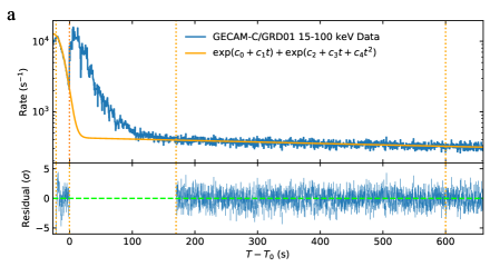
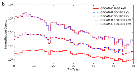
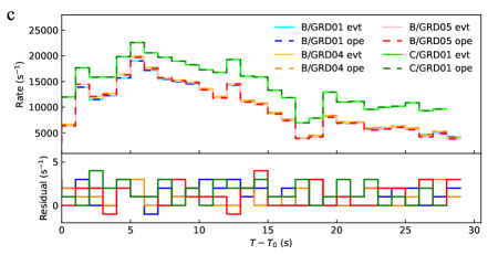
Figure 2: GECAM data reduction. a, The raw light curve of GECAM-C/GRD01 (blue solid line) and the background estimation (orange solid line). The light curve data points within the orange dashed line are used to fit the background model, then the background estimation can be obtained by interpolating the fitted model over the burst time interval. b, Comparison of the net light curves of GECAM-B and GECAM-C. The consistency between these two instruments validates the background estimation of GECAM-C. c, Comparison of recorded event rate (evt data, solid line) and processed event rate (ope engineering data, dashed line) of GECAM-B and GECAM-C for GRB 230307A. It is shown that the difference between these two event rates is negligible, demonstrating that both GECAM-B and GECAM-C have no data saturation for GRB 230307A.

The broad-band (0.5–6000 $\rm keV$, Methods) prompt emission data we have collected from GECAM and LEIA also independently point toward a compact star merger origin. The burst’s placement on various correlation diagrams is consistent with the so-called type I GRBs[25], i.e., those with a compact star merger origin (Methods and Fig. 2a-d). First, its relatively small minimum variability timescale is more consistent with type I GRBs. Second, it deviates from the Amati relation of type II GRBs (massive star core collapse origin) but firmly falls into the 1$\sigma$ scattering region of type I GRBs. Third, it is a significant outlier of the anti-correlation between the spectral lags and peak luminosities of type II GRBs but is mixed in with other type I GRBs. Besides, the optical host galaxy data[14] adds yet one more support: the location of the burst has a significant offset from the host galaxy, which is at odds with type II GRBs but is fully consistent with type I GRBs. This is the second strong instance for long-duration type I GRBs after GRB 211211A[26] (see also Fig. 2).

With the broad-band coverage jointly provided by GECAM-B/GECAM-C and LEIA throughout the prompt emission phase, one can perform a detailed temporal and spectral analysis of the data of GRB 230307A (Methods and Fig. 1). The light curves in the energy range of GECAM-B and GECAM-C exhibit synchronized pulses with matching peak and dip features (Fig. 1a). The time-resolved spectrum in the 15–6000 keV displays significant evolution (Fig. 1b and 1c), aligning with the “intensity tracking” pattern (i.e., the peak energy tracks the intensity’s evolution[27]). When plotting the energy flux light curves in the logarithmic-logarithmic space (Fig. 3a), a break is identified around 18–27 s post-trigger in all five GECAM bands (15–30 keV, 30–100 keV, 100–350 keV, 350–700 keV, and 700–2000 keV), after which the light curves decay with indices of $2.44_{-0.02}^{+0.02}$, $2.80_{-0.02}^{+0.02}$, $3.42_{-0.02}^{+0.02}$, $4.14_{-0.08}^{+0.08}$, and $4.59_{-0.17}^{+0.19}$ in these bands respectively (Methods). Compared with the theoretical prediction, a relation between the temporal decay slope and spectral slope solely due to the high-latitude emission effect after a sudden cessation of the emission (the so-called curvature effect[28]), these measured slopes are well consistent with the model’s prediction, suggesting that the prompt high-energy emission abruptly ceased or significantly reduced its emission amplitude at about 18–27 s post-trigger (Methods and Fig. 3c). There is an additional achromatic break around 84 s, after which the three light curves (15–30 keV, 30–100 keV, and 100–350 keV) decay with much steeper slopes (Methods and Fig. 3a,c). This is consistent with the edge effect of a narrow jet that powers the prompt $\gamma$-ray emission, with a half opening angle of $\sim 3.4^{\circ}(R_{\rm GRB}/10^{15}~{}{\rm cm})^{-1/2}$, where $R_{\rm GRB}$ is the unknown GRB prompt emission radius from the central engine (Methods). This brings the collimation-corrected jet energy to $\sim 5.4\times 10^{49}$ erg, typical to type I GRBs[29].

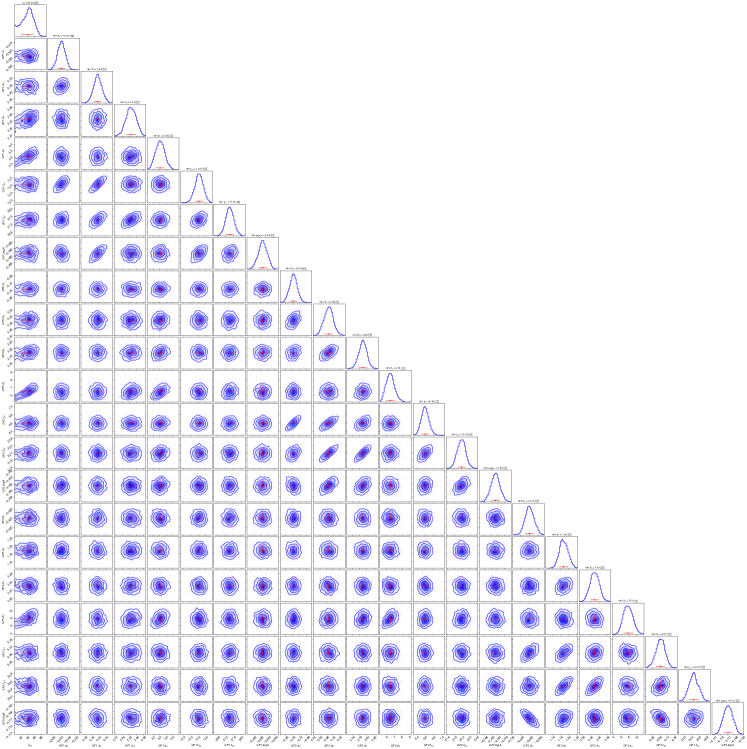
Figure 4: Corner plot of the posterior probability distributions of the parameters for the global fit to GECAM multi-wavelength (including 15–30, 30–100 and 100–350 keV, denoted by GF1, GF2 and GF3, respectively) flux light curves. The red error bars represent 1$\sigma$ uncertainties.

In contrast to the hard X-rays and gamma-rays, the soft X-ray emission in the 0.5–4 keV LEIA-band exhibits a different behavior. The emission sustains for a much longer duration of $>250$ s in the form of a plateau followed by a decline. Its spectrum shows much less significant evolution within the first 100 s (Fig. 1d and Extended Data Table 1) compared to the high-energy GECAM spectrum. Notably, its spectral shape from the beginning up to $\sim$75 s deviates strongly from the extrapolations to lower energies of the spectral energy distributions derived from the GECAM data (Methods and Fig. 3b). These deviations cannot easily be ascribed to a simple spectral break at low energies as sometimes seen in GRBs[30], but rather hint at a different radiation process dominating the LEIA band. As the high-energy emission suddenly ceases (with the decay slope controlled by the curvature effect), the late decay slope in the LEIA band is shallower than the curvature effect prediction, suggesting an intrinsic temporal evolution from the central engine (Fig. 3c). These facts suggest that the LEIA-band soft X-ray emission comes from a distinct emission component from the GRB, which emerges already from the onset of the burst (Fig. 3a). A smoothly broken power law fit to the light curve gives decay slopes of $0.40_{-0.06}^{+0.05}$ and $2.33_{-0.15}^{+0.16}$ before and after the break time at $79.90_{-5.78}^{+5.42}$ s (Methods and Fig. 4a). This pattern is generally consistent with the magnetic dipole spin-down law of a newborn, rapidly spinning magnetar. The best fit of the luminosity light curve with the magnetar model[3, 10] yields a dipole magnetic field of $2.21^{+0.54}_{-0.55}\times 10^{16}$ G, an initial spin period of $3.49^{+0.85}_{-0.89}$ ms, and a radiation efficiency of $6.11^{+2.02}_{-2.02}\times 10^{-3}$ (Methods and Fig. 4a). An X-ray plateau may also be interpreted within a black hole engine with a long-term accretion disk[31]. However, such a long-lived disk would be eventually quickly evaporated so that the jet engine would cease abruptly. The fact that the final decay slope of the LEIA light curve is shallower than the curvature effect prediction rules out such a possibility and reinforces the magnetar interpretation.

Indirect evidence of a magnetar engine in compact star mergers has been collected before in the form of internal plateaus in short GRBs[9, 10] and some short-GRB-less X-ray transients such as CDF-S XT2[11]. Fig. 4b shows the comparison of the X-ray luminosity light curves between GRB 230307A and other magnetar candidates. It shows that GRB 230307A is well consistent with the other sources but displays the full light curve right from the trigger, thanks to the prompt detection by the wide-field X-ray camera of LEIA. It reveals the details of the emergence of the magnetar emission component and lends further support to the magnetar interpretation of other events. In the near future, the synergy between GRB monitors and wide-field soft X-ray telescopes (such as the Einstein Probe) may detect more cases and will generally provide more observational information to diagnose the physics of GRBs during the prompt emission stage.

The identification of a magnetar engine from a merger event suggests that the neutron star equation of state is relatively stiff[7, 8]. It also challenges modelers who currently fail to generate a relativistic jet from new-born magnetars[13]. One possibility is that a highly magnetized jet is launched seconds after the birth of the magnetar when the proto-neutron star cools down and the wind becomes clean enough[5]. In any case, the concrete progenitor of GRB 230307A remains an enigma. With a magnetar engine the progenitor can only be a binary neutron star (NS) merger or a (near Chandrasekhar limit) white dwarf – NS merger[26]. For the former possibility, one must explain why this burst is particularly long. A “tip-of-icecube” test[32] suggests that it is hard to make this burst to be a bright short GRB when one arbitrarily raises the background flux or moves the source to higher redshift (Methods and Table 1). For the latter scenario, the fact that the light curves and spectral evolution between GRBs 230307A and 211211A[26] do not fully resemble each other would suggest that the mechanism must be able to produce diverse light curves. Unfortunately, GRB 230307A was detected prior to the fourth operation run (O4) of LIGO-Virgo-KAGRA. Future multi-messenger observations of similar events hold the promise of eventually unveiling the identity of the progenitor of these peculiar systems[33].

Table 1: Observational Properties. All errors represent the 1$\sigma$ uncertainties.

Observed Properties	GRB 230307A
Gamma-Ray [10–1000 keV]:
Duration (s)	$41.52\pm 0.03$
Effective amplitude	$1.23\pm 0.07$
Minimum variability timescale (ms)	$9.35$
Rest-frame spectral lag* (ms)	$1.6_{-1.2}^{+1.4}$
Spectral index $\alpha$	$-1.198_{-0.002}^{+0.003}$
Peak energy (keV)	$1254.68_{-17.99}^{+14.95}$
Peak flux ($\rm erg~{}cm^{-2}~{}s^{-1}$)	$4.48_{-0.12}^{+0.08}\times 10^{-4}$
Total fluence ($\rm erg~{}cm^{-2}$)	$(3.01\pm 0.01)\times 10^{-3}$
Peak luminosity ($\rm erg~{}s^{-1}$)	$4.89_{-0.13}^{+0.09}\times 10^{51}$
Isotropic energy (erg)	$(3.08\pm 0.01)\times 10^{52}$
Soft X-Ray [0.5–4 keV]:
Duration (s)	$199.6_{-2.2}^{+5.1}$
Spectral index $\alpha$	$-1.67_{-0.07}^{+0.06}$
Peak flux ($\rm erg~{}cm^{-2}~{}s^{-1}$)	$3.65_{-0.27}^{+0.33}\times 10^{-7}$
Total fluence ($\rm erg~{}cm^{-2}$)	$2.27_{-0.06}^{+0.07}\times 10^{-5}$
Peak luminosity ($\rm erg~{}s^{-1}$)	$3.97_{-0.29}^{+0.36}\times 10^{48}$
Isotropic energy (erg)	$2.47_{-0.06}^{+0.07}\times 10^{50}$
Host Galaxy:
Redshift	$0.065$
Half-light radius (kpc)	$4.0$
Offset (kpc)	$36.60$
Normalized offset	$9.2$
Probability of chance coincidence	$0.11$
Associations:
Kilonova	Yes
Supernova	No

• The rest-frame spectral lag is measured between rest-frame energy bands 100–150 and 200–250 keV.

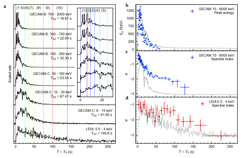
Figure 1: The temporal and spectral behaviors of GRB 230307A. a, The multi-wavelength net light curves of GRB 230307A. The Spectral Energy Distribution (SED) time intervals are demarcated by vertical dashed lines, accompanied by numerical labels at the top. Insets within the panel provide detailed profiles of prompt light curves in GECAM energy bands. b and c, The evolution of peak energy $E_{\rm p}$ and spectral power law index $\alpha$ derived from GECAM spectral fittings in 15–6000 $\rm keV$. d, The evolution of spectral power law index $\alpha$ derived from LEIA spectral fittings in 0.5–4 $\rm keV$. The light curves (gray lines) are plotted in the background as a reference. All error bars represent the 1$\sigma$ confidence level.

\begin{overpic}[width=195.12767pt]{Figure_2a.pdf}\put(2.0,80.0){\bf a}\end{overpic}	\begin{overpic}[width=195.12767pt]{Figure_2b.pdf}\put(2.0,80.0){\bf b}\end{overpic}
\begin{overpic}[width=195.12767pt]{Figure_2c.pdf}\put(2.0,80.0){\bf c}\end{overpic}	\begin{overpic}[width=195.12767pt]{Figure_2d.pdf}\put(2.0,80.0){\bf d}\end{overpic}

Figure 2: Position of GRB 230307A in various GRB classification schemes. a, The minimum variability timescale versus duration diagram. b, The rest-frame peak energy versus isotropic energy correlation diagram. The best-fit correlations and 1$\sigma$ regions of intrinsic scatter are presented by solid lines and shaded areas, respectively. c, The peak luminosity versus rest-frame lag diagram. The best-fit correlation and 1$\sigma$ region of intrinsic scatter for type II GRBs are presented by cyan line and shaded area, respectively. In a, b, and c, type I and type II GRBs are represented by grey and cyan solid circles, respectively. GRB 230307A ($z=0.065$) and GRB 211211A are highlighted by red and blue filled stars, respectively. GRB 230307A ($z=3.87$) is marked by a red unfilled star. d, The distribution of the physical offset of type I and type II GRBs from the center of the host galaxy[34]. GRB 230307A is overplotted in red, showing its consistency with type I GRBs. All error bars on data points represent their 1$\sigma$ confidence level.

\begin{overpic}[width=151.76964pt]{Figure_3a.pdf}\put(0.0,97.0){\bf a}\end{overpic}	\begin{overpic}[width=151.76964pt]{Figure_3b.pdf}\put(0.0,97.0){\bf b}\end{overpic}
\begin{overpic}[width=260.17464pt]{Figure_3c.pdf}\put(0.0,52.0){\bf c}\end{overpic}

Figure 3: The flux light curves and SEDs. a, The multi-wavelength flux light curves. The fluxes (data points) are derived from time-resolved spectral fittings, and the lines represent the best fits of smoothly broken power law functions to the multi-wavelength flux light curves. The grey shaded area marks the dip phase (17–20 s since trigger time). The orange shaded area represents the achromatic break in GECAM energy bands. b, The evolution of SEDs. The SEDs are derived from the spectral fittings at different time intervals as indicated by the labels. The dotted and dashed lines represent the natural extrapolations of the best-fit models of LEIA and GECAM independently spectral fittings, respectively. c, The temporal slopes. The data points and lines depict the slopes predicted by the high-latitude effect and the observed temporal slopes in each narrow energy band, respectively. All error bars on data points represent their 1$\sigma$ confidence level. All downward arrows represent the 3$\sigma$ upper limits. All shaded areas around the best-fit lines represent their 1$\sigma$ confidence bands.

\begin{overpic}[width=208.13574pt]{Figure_4a.pdf}\put(5.0,65.0){\bf a}\end{overpic}

\begin{overpic}[width=208.13574pt]{Figure_4b.pdf}\put(0.0,65.0){\bf b}\end{overpic}

Figure 4: X-ray luminosity light curve of GRB 230307A. a, The unabsorbed X-ray luminosity light curve in the energy range of $0.5-4$ $\rm keV$ is fitted using both the smoothly broken power law model and the magnetar dipole radiation model, as described in Methods. The shaded area represents the 1$\sigma$ confidence bands. b, In comparison with the X-ray afterglows of the internal plateau sample in short GRBs[10] (gray) and CDF-S XT2. X-ray afterglow of GRB 230307A detected by Swift/XRT is corrected to the same energy band and represented with the unfilled red star.

Methods

0.1 Multi-mission observations of GRB 230307A

GRB 230307A triggered in real-time the Gravitational wave high-energy Electromagnetic Counterpart All-sky Monitor (GECAM) and the Fermi Gamma-ray Burst Monitor (GBM) almost simultaneously. The extreme brightness of GRB 230307A was first reported by GECAM-B with its real-time alert data downlinked by the Beidou satellite navigation system[17], which was subsequently confirmed by Fermi/GBM[35, 36] and Konus-Wind[37]. Preliminary location of this burst measured by GECAM is consistent with that of GBM within error[17]. Refined localization in gamma-ray band was provided by the Inter-Planetary Network (IPN) triangulation[38] and later improved by follow-up observations of the X-ray Telescope (XRT) aboard the Neil Gehrels Swift Observatory[39, 40]. The Lobster Eye Imager for Astronomy (LEIA) detected the prompt emission of this burst in the 0.5–4 keV soft X-ray band[23]. The burst was also followed up by the Gemini-South[41, 42] and the James Webb Space Telescope (JWST) at several epochs[43, 44, 45], unveiling a fading afterglow with possible signatures of kilonova in the optical and infrared bands and a candidate host galaxy at a redshift of $z=0.065$[14] (Table 1).

0.2 Data reduction

LEIA. The Lobster Eye Imager for Astronomy[21, 22], a pathfinder of the Einstein Probe mission of the Chinese Academy of Sciences, is a wide-field ($18.6^{\circ}\times 18.6^{\circ}$) X-ray focusing telescope built from novel technology of lobster eye micro-pore optics. The instrument operates in the 0.5–4 keV soft X-ray band, with an energy resolution of 130 eV (at 1.25 keV) and a time resolution of 50 ms. LEIA is onboard the Space Advanced Technology demonstration satellite (SATech-01), which was launched on 2022 July 27 and is operating in a Sun-synchronous orbit with an altitude of 500 $\rm km$ and an inclination of $97.4^{\circ}$. Since LEIA operates only in the Earth’s shadow to eliminate the effects of the Sun, the observable time out of the radiation belt at high geo-latitude regions is $\sim$1000 s for each orbit. The observation of GRB 230307A was conducted from 15:42:32 UT (94 s earlier than the GECAM trigger time) to 16:00:50 UT on 7 March 2023 with a net exposure of 761 s. GRB 230307A was detected within the extended field of view (about $0.6^{\circ}$ outside the nominal field of view) of LEIA[23](Extended data Fig. 1).

The X-ray photon events were processed and calibrated using the data reduction software and calibration database (CALDB) designed for the Einstein Probe mission (Liu et al. in prep.). The CALDB is generated based on the results of on-ground and in-orbit calibration campaigns (Cheng et al. in prep.). The energy of each event was corrected using the bias and gain stored in CALDB. Bad/flaring pixels were also flagged. Single-, double-, triple-, and quadruple-events without anomalous flags were selected to form the cleaned event file. The image in the 0.5–4 keV range was extracted from the cleaned events (Extended Data Fig. 1a). The position of each photon was projected into celestial coordinates (J2000). The light curve and the spectrum of the source and background in a given time interval were extracted from the regions indicated in Extended Data Fig. 1a. Since the peak count rate is only 2 ct/frame over the extended source region, the pile-up effect is negligible in the LEIA data.

GECAM. GECAM is a dedicated all-sky gamma-ray monitor constellation funded by the Chinese Academy of Sciences. The original GECAM mission[15] is composed of two microsatellites (GECAM-A and GECAM-B) launched in December 2020. GECAM-C[16] is the 3rd GECAM spacecraft, also onboard the SATech-01 satellite as LEIA. Each GECAM spacecraft has an all-sky field of view unblocked by the Earth, capable of triggering bursts in real-time[46] and distributing trigger alerts promptly with the Global Short Message Communication of Beidou satellite navigation system[47]. As the main instrument of GECAM, most gamma-ray detectors (GRDs) operate in two readout channels: high gain (HG) and low gain (LG), which are independent in terms of data processing, transmission, and dead-time[48]. Comprehensive ground and cross calibrations have been conducted on the GRDs of both GECAM-B and GECAM-C[49, 16, 50, 51].

GRB 230307A was detected by GECAM-B and GECAM-C, while GECAM-A was offline. GECAM-B was triggered by this burst and automatically distributed a trigger alert to GCN Notice about 1 minute post-trigger. GECAM-C also made the real-time trigger onboard, while the trigger alert was disabled due to the high latitude region setting[16]. With the automatic pipeline processing the GECAM-B real-time alert data (Huang et al. RAA, in press), we promptly noticed and reported that this burst features an extreme brightness[17], which initiated the follow-up observations.

Both GECAM-B and GECAM-C were working in inertial pointing mode during the course of GRB 230307A. Among all 25 GRDs of GECAM-B, GRD04 maintains a constant minimum zenith angle of $12.7^{\circ}$ throughout the duration of the burst. GRD01 and GRD05 also exhibit small zenith angles of $32.4^{\circ}$ and $32.7^{\circ}$, respectively. Thus these three detectors are selected for subsequent analysis. For GECAM-B GRDs, the HG channel operates from $\sim$ 40 to 350 keV, while the LG channel from $\sim$ 700 keV to 6 MeV. Among all 12 GRDs of GECAM-C, GRD01 exhibits the most optimal incident angle of $10.1^{\circ}$ throughout the burst and is selected in the subsequent analysis. For GECAM-C/GRD01, the HG channel operates from $\sim$ 6 to 350 keV. Since the detector response for 6–15 keV is affected by the electronics and is subject to further verification[51], we only use $>$15 keV for spectral analysis in this work. The background estimation methodology employed for GECAM-C/GRD01 involves fitting a combination of first and second-order exponential polynomials to the adjacent background data, followed by interpolating the background model to the time intervals of the burst (Extended Data Fig. 2a). The efficacy of this background estimation for GECAM-C/GRD01 is verified by the comparison with GECAM-B data (Extended Data Fig. 2b).

We note that GRB 230307A was so bright that the Fermi/GBM observation suffered from data saturation[52]. GECAM has dedicated designs to minimize data saturation for bright bursts[15, 53]. For GECAM, the engineering count rate records the number of events processed onboard, while the event count rate records the number of events received on ground. In the case of data saturation, these two count rates would differ significantly. As shown in Extended Data Fig. 2c, the negligible discrepancy between these two count rates, due to the limited digital accuracy on the count numbering, confirms no count loss in event data and indicates the absence of saturation for both GECAM-B and GECAM-C.

0.3 Temporal analysis

Duration. The light curves are obtained through the process of photon counts binning (Fig. 1). The light curve for LEIA is obtained in 0.5–4 $\rm keV$ with a bin size of 1 s. The light curves for GECAM-B are generated using the bin size of 0.4 s in the energy ranges of 100–350 $\rm keV$, 350–700 $\rm keV$, and 700–2000 $\rm keV$, by combining the data from three selected detectors (namely, GRD01, GRD04, and GRD05). The GECAM-C light curves are derived by binning the photon counts from GRD01 with a bin size of 0.4 s in the energy ranges of 6–15 $\rm keV$, 15–30 $\rm keV$, and 30–100 $\rm keV$. The burst duration, denoted as $T_{\rm 90}$, is determined by calculating the time interval between the epochs when the total accumulated net photon counts reach the $5\%$ and $95\%$ levels. The durations obtained from the multi-wavelength light curve are annotated in Fig. 1. It is found that the duration of the burst significantly increases towards the lower energy range. We also calculate the duration within 10–1000 $\rm keV$ based on the data from GECAM-B and list it in Table 1.

Amplitude parameter. The amplitude parameter[32] is a metric used to classify GRBs and is defined as $f=F_{\rm p}/F_{\rm b}$, denoting the ratio between the peak flux $F_{\rm p}$ and the background flux $F_{\rm b}$ at the same time epoch. A long-duration type II GRB may be disguised as a short-duration type I GRB due to the tip-of-iceberg effect. To distinguish intrinsically short-duration type I GRBs from ostensible short-duration type II GRBs, an effective amplitude parameter, $f_{\rm eff}=\epsilon f=F_{\rm p}^{\prime}/F_{\rm b}$, can be defined for long-duration type II GRBs by quantifying the tip-of-iceberg effect, where $F_{\rm p}^{\prime}$ is the peak flux of a pseudo GRB whose amplitude is lower by a factor $\epsilon$ from an original long-duration type II GRB so that its duration is just shorter than 2 s. Generally speaking, the $f_{\rm eff}$ values of long-duration type II GRBs are systematically smaller than the $f$ values of short-duration type I GRBs, thereby facilitating their distinction from one another. Utilizing the procedure presented in Ref.[32], the effective amplitude of GRB 230307A is determined to be $f_{\rm eff}=1.23\pm 0.07$ within the energy range of 10–1000 keV (Table 1). Such small $f_{\rm eff}$ value aligns with the characteristics typically exhibited by long-duration GRBs.

Variability. The minimum variability timescale (MVT) is defined as the shortest timescale of significant variation that exceeds statistical noise in the GRB temporal profile[54, 55]. It serves as an indicator of both the central engine’s activity characteristics and the geometric dimensions of the emitting region. The median values of the minimum variability timescale in the rest frame (i.e., MVT$/(1+z)$) for type I and type II GRBs are found to be 10 ms and 45 ms, respectively. To determine the MVT, we utilize the Bayesian block algorithm[56] on the entire light curve within the 10–1000 keV energy range to identify the shortest block that satisfies the criterion of encompassing the rising phase of a pulse. We find that the MVT of GRB 230307A is about 9.35 ms (Table 1), which is more consistent with type I GRBs rather than type II GRBs in the distribution of the MVTs[54] (Fig. 2a). We also utilize the continuous wavelet transform (CWT) method to derive MVT and obtain a consistent outcome in accordance with the Bayesian block algorithm.

Spectral lag. Spectral lag refers to the time delay between the soft-band and hard-band background-subtracted light curves. It may be attributed to the curvature effect in the relativistic outflow. Upon reaching the observer, on-axis photons are boosted to higher energies, while off-axis photons receive a smaller boost and must travel a longer distance. Type II GRBs usually exhibit considerable spectral lags, while type I GRBs tend to have tiny lags[57, 58], indicating the difference in their emission region sizes. Measurement of the spectral lag can be achieved by determining the time delay corresponding to the maximum value of the cross-correlation function[59, 60, 61]. Following the treatment in Ref.[60], we use the background-subtracted light curves of GRB 230307A to measure the rest-frame lag between rest-frame energy bands 100–150 and 200–250 keV to be $1.6_{-1.2}^{+1.4}$ ms (Table 1). We note that GRB 230307A manifests a very tiny spectral lag, an indicator that points towards being a type I GRB (Fig. 2c).

0.4 Spectral analysis

LEIA spectral fitting. We perform a detailed spectral analysis using the LEIA data. The energy channels in the range of 0.5–4 keV are utilized and re-binned to ensure that each energy bin contains at least ten counts. We employ three kinds of time segmentation approaches to extract LEIA spectra:

• LEIA S-I: the time interval from 0 to 200 s is divided into three slices (0–50 s, 50–100 s, 100–200 s) to investigate the possible evolution of X-ray absorption;

• LEIA S-II: 23 time slices with sufficient time resolution are obtained by accumulating 100 photon counts for each individual slice;

• LEIA S-III: the time interval from 0 to 140 s is divided into ten distinct time slices. This partitioning is designed to align with the temporal divisions of the GECAM spectra, enabling subsequent comparisons and joint spectral fitting.

For each of the above time slices, we generate the source spectrum and background spectrum, and the corresponding detector redistribution matrix and the ancillary response. First, the spectra of LEIA S-I are individually fitted with the XSPEC[62] model phabs*zphabs*zpowerlw, where the first and second components are responsible for the Galactic absorption and intrinsic absorption ($N_{\rm H}$), and the third one is a redshift-corrected power law function. We employ CSTAT[63] as the statistical metric to evaluate the likelihood of LEIA spectral fitting where both the source and background spectra are Poisson-distributed data. The column density of the Galactic absorption in the direction of the burst is fixed at $9.41\times 10^{20}~{}{\rm cm^{-2}}$[64] and the redshift is fixed at 0.065. It is found that all three spectra of S-I can be reproduced reasonably well by the absorption modified power law model (Extended Data Fig. 1b). The best-fit values and confidence contours of the column density and photon index are shown in Extended Data Fig. 1c. The fitted column densities are generally consistent within their uncertainties, indicating no significant variations of the absorption feature within 200 s. A time-averaged absorption of $N_{\rm H}=2.73\times 10^{21}~{}{\rm cm^{-2}}$, yielded from the simultaneous fitting of all three S-I spectra, is thus adopted and fixed in all subsequent spectral analysis.

We then proceed with the fitting of the LEIA S-II spectra. The obtained results for the photon index ($\Gamma_{\rm ph}$), normalization, and the corresponding fitting statistic are presented in Extended Data Table 1. By employing a redshift of $z=0.065$, we further calculated the unabsorbed flux (Fig. 3a) and determined the luminosity for each S-II spectrum (Fig. 4a,b). Additionally, we cross-validated our findings by analyzing spectra with higher photon statistics, specifically 200 photons per time bin, and found that the alternate spectra yielded consistent results in our analysis. We also perform a spectral fit to the time-averaged spectrum during the whole observation interval of S-II, and the derived power-law index ($\alpha=-\Gamma_{\rm ph}$) is shown in Table 1. Finally, the LEIA S-III spectra are employed for SED analysis.

GECAM spectral fitting. We conduct a thorough time-resolved and time-integrated spectral analysis using the data from the GRD04 and GRD01 of GECAM-B, as well as the GRD01 of GECAM-C. Each GRD detector has two independent readout channels, namely, high gain (HG) and low gain (LG). We utilize both the high and low gain data of the GECAM-B detectors with effective energy ranges of 40–350 and 700–6000 keV, respectively. Additionally, we only used the high gain data of the GECAM-C detector with an effective energy range of 15–100 keV but ignored the channels within 35–42 keV around the Iodine K-edge at 38.9 keV. We employ three distinct time segmentation methods over the time interval of 0–140 s:

• GECAM S-I: the entire time interval is treated as a single time slice for time-integrated spectral analysis;

• GECAM S-II: the time interval is divided into 99 time slices with sufficient spectral resolutions and approximately equal signal-to-noise levels;

• GECAM S-III: the time interval is partitioned into ten time slices to match the time division of LEIA spectra for comparison and joint fitting.

For each of the above time slices, we generate a source spectrum, a background spectrum, and a response matrix for each gain mode of each detector. Then we perform spectral fitting by utilizing the Python package, MySpecFit, in accordance with the methodology outlined in Refs.[26, 65]. The MySpecFit package facilitates Bayesian parameter estimation by wrapping the widely-used Fortran nested sampling implementation Multinest[66, 67, 68, 69]. PGSTAT[62] is utilized for GECAM spectral fitting, which is appropriate for Poisson data in the source spectrum with Gaussian background in the background spectrum. The cutoff power law (CPL) model is adopted to fit GECAM S-I and S-II spectra. The CPL model can be expressed as

$$N(E)=A(\frac{E}{100\,{\rm keV}})^{\alpha}{\rm exp}(-\frac{E}{E_{\rm c}}),$$ (1)

where $\alpha$ is low-energy photon spectral index, and $A$ is the normalization parameter in units of ${\rm photons~{}cm^{-2}~{}s^{-1}~{}keV^{-1}}$. The peak energy $E_{\rm p}$ of $\nu f_{\nu}$ spectrum is related to the cutoff energy $E_{\rm c}$ through $E_{\rm p}=(2+\alpha)E_{\rm c}$. Extended Data Table LABEL:tab:gecam_spec_fit lists the spectral fitting results and corresponding fitting statistics for GECAM S-I and S-II spectra. It should be noted that we use cutoff energy as a substitute for peak energy when the 1$\sigma$ lower limit of $\alpha$ falls below $-2$. Fig. 1b and 1c illustrate the significant “intensity tracking” spectral evolution in terms of $E_{\rm p}$ and $\alpha$, respectively.

Spectral energy distribution. We perform spectral fitting on the spectra of LIEA S-III and GECAM S-III to examine the spectral energy distribution (SED) from soft X-rays to gamma-rays. To avoid the imbalance in fitting weights to lose spectral information due to significant differences in the fitting statistics between LEIA and GECAM, we first fit the spectra of LEIA and GECAM independently. For the LEIA S-III spectral fitting, we still employ the redshift-corrected power-law (PL) model with Galactic absorption (fixed to a hydrogen column density of $9.41\times 10^{20}~{}{\rm cm^{-2}}$) and intrinsic absorption (fixed to a hydrogen column density of $2.73\times 10^{21}~{}{\rm cm^{-2}}$). The PL model is defined as:

$$N(E)=A(\frac{E}{100\,{\rm keV}})^{\alpha},$$ (2)

where $\alpha$ is low-energy photon spectral index, and $A$ is the normalization parameter in units of ${\rm photons~{}cm^{-2}~{}s^{-1}~{}keV^{-1}}$. For the GECAM S-III spectral fitting, we adopt the redshift-corrected CPL model, except for the three time slices of 13–18 s, 18–25 s, and 25–35 s, which require an additional cutoff and power law function below $\sim 50$ keV in the model. Therefore, we employ the redshift-corrected BAND-Cut model[70] to fit the three time slices. The BAND-Cut model is defined as

$$N(E)=\left\{\begin{array}[]{l}AE^{\alpha_{1}}{\rm exp}(-\frac{E}{E_{1}}),~{}E\leq E_{\rm b},\\ AE_{\rm b}^{\alpha_{1}-\alpha_{2}}{\rm exp}(\alpha_{2}-\alpha_{1})E^{\alpha_{2}}{\rm exp}(-\frac{E}{E_{2}}),~{}E>E_{\rm b},\\ \end{array}\right.$$ (3)

where $\alpha_{1}$ and $\alpha_{2}$ represent the spectral indices of the two low-energy power law segments smoothly connected at the break energy $E_{\rm b}=\frac{E_{1}E_{2}}{E_{2}-E_{1}}(\alpha_{1}-\alpha_{2})$, $A$ is the normalization parameter in units of ${\rm photons~{}cm^{-2}~{}s^{-1}~{}keV^{-1}}$. The peak energy of $\nu f_{\nu}$ spectrum is defined as $E_{\rm p}=E_{2}(2+\alpha_{2})$, which locates at the high-energy exponential cutoff.

The spectral fitting results, along with the corresponding fitting statistics, are represented in Extended Data Table 3. The comparison between observed and model-predicted count spectra and the residuals (defined as $({\rm data}-{\rm model})/{\rm data~{}error}$) is depicted in Extended Data Fig. 3a. The SEDs derived from the spectral fittings at different time intervals are displayed in Fig. 3b. We notice that, in the early time intervals (before about 75 s), the PL spectra of LEIA (0.5–4 keV) and CPL or BAND-Cut spectra of GECAM (15–6000 keV) do not align with the natural extrapolation of each other (Fig. 3b). This is mainly manifested by significant differences in the spectral index and amplitude of the LEIA and GECAM spectra. Such inconsistency suggests the presence of two distinct prompt emission components, each dominating the spectra of LEIA and GECAM, respectively. We also note that in the last two time slices, the spectra from both instruments can be seamlessly connected and adequately described by a single CPL model (Extended Data Fig. 3a and Fig. 3b), indicating that in the later stages (after approximately 75 s), a single component progressively dominates the spectra from both instruments.

Another approach to demonstrate the SED involves combining the LEIA S-III and GECAM S-III spectra to perform a joint fitting. We initially adopt the redshift-corrected CPL model for joint fitting, but for certain time intervals, an additional spectral cutoff and power law function need to be introduced in the low-energy range of the CPL model to connect both LEIA and GECAM spectra, for which we consider the redshift-corrected BAND-Cut model. When both the CPL and BAND-Cut models can be constrained, the model comparison is performed based on the Bayesian information criterion[71] (defined as ${\rm BIC}=-2{\rm ln}\mathcal{L}+k{\rm ln}N$, where $\mathcal{L}$ is the maximum likelihood value, $k$ is the number of model’s free parameters, and $N$ is the number of data points), where a model with a smaller BIC value is preferred. Extended Data Table 3 represents the fitting results of the preferred models and corresponding statistics. The comparison between observed and model-predicted count spectra and the residuals are represented in Extended Data Fig. 3b. The SEDs derived from the joint spectral fittings at different time intervals are displayed in Extended Data Fig. 3c. Considering the possibility of the model overlooking some spectral features in the soft X-ray band due to the significantly lower contribution of LEIA data to the fitting statistics, we overlay the model-predicted count spectra and SEDs obtained from the independent LEIA fittings onto Extended Data Fig. 3b and 3c, respectively. The comparison between the joint SEDs and the independent LEIA SEDs further confirms that, in the early stage (before about 75 s), even with the introduction of an additional break and power law at low energies, the model still can not account for the unique spectral features of LEIA, which once again points to the conclusion of two distinct components. In contrast, the consistency between the joint SEDs and LEIA independent SEDs in the late stage (after about 75 s) suggests a single dominant component.

0.5 Classification

Variability timescale versus duration. The temporal variability timescale of GRBs may conceal imprints of central engine activity and energy dissipation processes. On average, the minimum variability timescale of short-duration type I GRBs is significantly shorter than that of long-duration type II GRBs, providing a new clue to distinguish the nature of GRB progenitors and central engines[54, 55]. We collected previous research samples, redrawn the ${\rm MVT}-T_{\rm 90}$ diagram, and overlaid GRB 230307A and GRB 211211A on it (Fig. 2a). It is noteworthy that these two GRBs are outliers, as their MVTs are more consistent with that of type I GRBs despite being long-duration GRBs.

Peak energy versus isotropic energy. The $E_{\rm p,z}-E_{\rm\gamma,iso}$ diagram serves as a unique classification scheme in the study of GRB energy characteristics, as different physical origins of GRBs typically follow distinct tracks[72, 25, 73]. We first replot the $E_{\rm p,z}-E_{\rm\gamma,iso}$ diagram (Fig. 2b) based on previous samples of type I and type II GRBs with known redshifts[73]. Here, $E_{\rm p,z}=E_{\rm p}(1+z)$ represents the rest-frame peak energy, while $E_{\rm\gamma,iso}$ denotes the isotropic energy. The relations between $E_{\rm p,z}$ and $E_{\rm\gamma,iso}$ can be modeled using a linear relationship, ${\rm log}E_{\rm p,z}=b+k{\rm log}E_{\rm\gamma,iso}$, for both GRB samples. The fitting process is implemented using the Python module emcee[74], and the likelihood is determined using the orthogonal-distance-regression (ODR) method[75]. The ODR method is appropriate in this case as the data satisfy two criteria: (1) a Gaussian intrinsic scatter $\sigma_{\rm int}$ along the perpendicular direction; (2) independent errors $\sigma_{x_{i}}$ and $\sigma_{y_{i}}$ on both the $x$ and $y$ axes. The log-likelihood function can be expressed as

$${\rm ln}\mathcal{L}=-\frac{1}{2}\sum_{i}\Big{[}{\rm ln}(2\pi\sigma_{i}^{2})+\frac{\Delta_{i}^{2}}{\sigma_{i}^{2}}\Big{]},$$ (4)

with the perpendicular distance

$$\Delta_{i}^{2}=\frac{(y_{i}-kx_{i}-b)^{2}}{k^{2}+1},$$ (5)

and the total perpendicular uncertainties

$$\sigma_{i}^{2}=\frac{k^{2}\sigma_{x_{i}}^{2}+\sigma_{y_{i}}^{2}}{k^{2}+1}+\sigma_{\rm int}^{2},$$ (6)

where the subscript $i$ runs over all data points. The best-fitting parameters with 1$\sigma$ uncertainties are $k=0.36_{-0.05}^{+0.04}$, $b=-15.61_{-2.14}^{+2.51}$ and ${\rm log}\sigma_{\rm int}=-1.29_{-0.13}^{+0.13}$ for type I GRBs, and $k=0.39_{-0.02}^{+0.02}$, $b=-17.82_{-0.98}^{+0.93}$ and ${\rm log}\sigma_{\rm int}=-1.42_{-0.05}^{+0.05}$ for type II GRBs. The best-fit correlations and corresponding 1$\sigma$ intrinsic scattering regions are presented in Fig. 2b. The peak energy of GRB 230307A is constrained to be $E_{\rm p}=1254.68_{-17.99}^{+14.95}$ keV by the spectral fitting to GECAM S-I. Given a redshift of 0.065, the isotropic energy of GRB 230307A can be calculated as $E_{\rm\gamma,iso}=(3.08\pm 0.01)\times 10^{52}$ erg. We overplot both long-duration GRB 230307A and GRB 211211A on the $E_{\rm p,z}-E_{\rm\gamma,iso}$ diagram. As can be seen from Fig. 2b, GRB 211211A resides in an intermediate area between the tracks of type I and type II GRBs, while GRB 230307A is firmly located within the 1$\sigma$ region of the type I GRB track. In addition, GRB 230307A poses higher total energy and harder spectra, likely indicating a more intense merger event. We also consider the scenario where the host galaxy has a redshift of 3.87[45] and notice that in this case, the isotropic energy of GRB 230307A is $\sim 10^{56}$ erg, which is an order of magnitude larger than that of the brightest-of-all-time GRB 221009A[65, 19]. Such extremely high energy is very unlikely consistent with the known sample of GRBs.

Peak luminosity versus spectral lag. An anti-correlation exists between the spectral lag and peak luminosity in the sample of type II GRB with a positive spectral lag[59, 60]. Such anti-correlation can serve as a physically ambiguous indicator, suggesting that GRBs with short spectral lags have higher peak luminosities. In general, type I GRBs deviate from the anti-correlation of type II GRBs, with type I GRBs tending to exhibit smaller spectral lags than type II GRBs at the same peak luminosity. The significant differences between the two in this regard make the peak luminosity versus spectral lag correlation a useful classification scheme. On the basis of the previous samples of type I and type II GRBs with known redshift[76, 60, 77], we replot the $L_{\rm\gamma,iso}-\tau_{\rm z}$ diagram, where $L_{\rm\gamma,iso}$ is isotropic peak luminosity and $\tau_{\rm z}=\tau/(1+z)$ is the rest-frame spectral lag (Fig. 2c). The anti-correlation between $L_{\rm\gamma,iso}$ and $\tau_{\rm z}$ for type II GRBs can be fit with the linear model ${\rm log}L_{\rm\gamma,iso}=b+k{\rm log}\tau_{\rm z}$. The ODR method[75] gives the best-fitting parameters with 1$\sigma$ uncertainties to be $k=-0.94_{-0.26}^{+0.07}$, $b=54.24_{-0.14}^{+0.49}$ and ${\rm log}\sigma_{\rm int}=-1.61_{-0.17}^{+0.29}$. To maintain consistency with the calculation method of the sample, we estimate the rest-frame lag of GRB 230307A between rest-frame energy bands 100–150 and 200–250 keV to be $1.6_{-1.2}^{+1.4}$ ms. Assuming the redshift to be 0.065, the isotropic peak luminosity of GRB 230307A can be calculated as $L_{\rm\gamma,iso}=4.89_{-0.13}^{+0.09}\times 10^{51}$ erg based on the spectral fits to GECAM S-II. Then we place both GRB 230307A and GRB 211211A on the $L_{\rm\gamma,iso}-\tau_{\rm z}$ diagram. As can be seen from Fig. 2c, their locations are more consistent with that of type I GRBs despite being long-duration GRBs. We also note that, if the redshift is 3.87[45], the extremely high peak luminosity of GRB 230307A would make it a significant outlier in the known sample of GRBs.

0.6 Fit of multi-wavelength flux light curves

On the basis of detailed spectral fitting to the time-resolved spectra of LEIA S-II and GECAM S-II, we calculate the energy flux for each time slice and construct the multi-wavelength flux light curves for six energy bands. These six energy bands, including 0.5–4, 15–30, 30–100, 100–350, 350–700, and 700–2000 keV, are set by referencing the effective energy ranges of the LEIA, GECAM-B, and GECAM-C. It is noteworthy that, during the last three time slices of GECAM S-II, only the high gain data from GECAM-C and GECAM-B exhibit effective spectra that are significantly above the background level, while the low gain data from GECAM-B are already close to the background level and do not provide effective spectral information, which leads to insufficient confidence in determining flux values in the energy bands above 350 keV. Therefore, based on the Bayesian posterior probability distribution generated by Multinest[66, 67, 68, 69], we provide the 3$\sigma$ upper limits of flux for 350–700 and 700–2000 keV in the last three time intervals. The multi-wavelength flux light curves are represented in Fig. 3a. All these flux light curves display multi-segment broken power law features. To fit these features, we introduce multi-segment smoothly broken power law (SBPL) functions.

In general, smoothly connected functions in a logarithmic-logarithmic scale can be expressed as

$$F=(F_{\rm l}^{-\omega}+F_{\rm r}^{-\omega})^{-1/\omega},$$ (7)

where $F_{\rm l}$ and $F_{\rm r}$ are the functions located on the left and right sides respectively, and $\omega$ describes the smoothness. When both of $F_{\rm l}$ and $F_{\rm r}$ are power law functions, a two-segment SBPL function can be obtained as

$$F_{12}=(F_{1}^{-\omega_{1}}+F_{2}^{-\omega_{1}})^{-1/\omega_{1}},$$ (8)

where $F_{1}=A(t/t_{\rm b1})^{-\alpha_{1}}$, $F_{2}=A(t/t_{\rm b1})^{-\alpha_{2}}$. The power law slopes before and after the break time $t_{\rm b1}$ are $\alpha_{1}$ and $\alpha_{2}$, respectively, and $A$ is the normalization coefficient at $t_{\rm b1}$. In the case where another break occurs after two-segment SBPL function, a three-segment SBPL function can be expressed as

$$F_{123}=(F_{12}^{-\omega_{2}}+F_{3}^{-\omega_{2}})^{-1/\omega_{2}},$$ (9)

where $F_{3}=F_{12}(t_{\rm b2})(t/t_{\rm b2})^{-\alpha_{3}}$ describes the third power law function. By extension, we can further expand the three-segment SBPL to include a third break and a forth power law function, namely the four-segment SBPL function:

$$F_{1234}=(F_{123}^{-\omega_{3}}+F_{4}^{-\omega_{3}})^{-1/\omega_{3}},$$ (10)

where $F_{4}=F_{123}(t_{\rm b3})(t/t_{\rm b3})^{-\alpha_{4}}$ describes the forth power law function.

The fitting process is implemented by the Python module PyMultinest[68], a Python interface to the widely-used Fortran nested sampling implementation Multinest[66, 67, 68, 69]. We employ $\chi^{2}$ as the statistical metric to evaluate the likelihood. It should be noted that a dip covering 17–20 s exists in the flux light curves of all energy bands of GECAM. Since the dip is an additional component superimposed on the multi-segment broken power law, the time interval containing the dip is omitted from the fitting procedure and will be examined in a separate analysis, which will be discussed in detail elsewhere. For convenience, we refer to the flux light curves of the six energy bands as LF (0.5–4 keV) and GFi (where i ranges from 1 to 5, representing the five energy bands of GECAM from low to high). We note that LF consists of a shallow power law decay followed by a steeper decline, which is significantly different from GFs, where they include an initial power law rise and several gradually steepening power law decay phases. GF1-3 require the four-segment SBPL functions to describe their features, while GF4 and GF5 can be described using three-segment SBPL functions as the late-time features cannot be constrained due to the last three data points being 3$\sigma$ upper limits. Interestingly, in the GECAM energy bands, the first three power law segments and the corresponding two break times exhibit clear spectral evolution features. From low to high energy, the power law decay index gradually increases, while the break times gradually shift to earlier times. However, the final breaks in GF1-3 appear to be a simultaneous feature. Such an achromatic break is typically attributed to the geometric effects of the emission region.

To test the simultaneity of the final break and determine its break time, we performed a joint fit to GF1-3. The fitting process can be described as follows. We simultaneously use three four-segment SBPL functions to fit GF1, GF2, and GF3 independently but allow the three $t_{\rm b3}$ parameters to degenerate into a common parameter. The statistic of the joint fit is the sum of $\chi^{2}$ values for GF1-3. The fitting process is also implemented by the Python module PyMultinest[68]. The best-fitting parameter values and their 1$\sigma$ uncertainties are presented in Extended Data Table 4. Extended Data Fig. 4 exhibits the corresponding corner plot of posterior probability distributions of the parameters for the joint fit, where all the parameters are well constrained, and the common parameter $t_{\rm b3}$ is also well constrained to be $84.05_{-2.19}^{+1.66}$ s.

0.7 Curvature effect

The “curvature effect” refers to the phenomenon of photons arriving progressively later at the observer from higher latitudes with respect to the line of sight[28, 78]. It has been proposed that this effect plays an important role in shaping the decay phase of the light curve after the sudden cessation of the GRB’s emitting shell[79, 80]. By assuming a power law spectrum with spectral index $\hat{\beta}$ for the GRB, the most straightforward relation of the curvature effect can be given as $\hat{\alpha}=2+\hat{\beta}$[28, 78, 81], where $\hat{\alpha}$ and $\hat{\beta}$ are the temporal decay index and spectral index in the convention $F_{\rm\nu}\propto t^{-\hat{\alpha}}\nu^{-\hat{\beta}}$, respectively. If the aforementioned assumptions are released, and the intrinsically curved spectral shape and strong spectral evolution are taken into account, the above relationship is no longer applicable[82, 83]. Nevertheless, for a narrow energy band, the intrinsically curved spectrum can be approximated, on average, by a power law, and the time-dependent $\hat{\alpha}$ and $\hat{\beta}$ still approximately follow the relation $\hat{\alpha}(t)=2+\hat{\beta}(t)$[83].

The multi-wavelength flux light curves of GRB 230307A exhibit an initial rise and subsequent power law decay phases that gradually become steeper. To test whether the decay phases are dominated by the curvature effect, we compare the time-dependent $\hat{\alpha}(t)$ and $2+\hat{\beta}(t)$ in each narrow energy band. Here, $\hat{\alpha}(t)$ is obtained by numerically calculating $-\Delta{\rm log}F/\Delta{\rm log}t$ of the best-fitting SBPL functions, while $\hat{\beta}(t)$ is the average spectral index $-\Delta{\rm log}F_{\rm\nu}/\Delta{\rm log}E$ calculated in the corresponding narrow energy band based on the spectral fitting results for each time slice of LEIA S-II or GECAM S-II. Fig. 3c displays the time-dependent $\hat{\alpha}(t)$ and $2+\hat{\beta}(t)$ for each energy band. We note that the power law decay indices of the segments between the second and third breaks (see $t_{\rm b2}$ and $t_{\rm b3}$ in Extended Data Table 4) of GECAM multi-wavelength flux light curves are consistent with the prediction of curvature effect, implying that the jet’s emitting shell stops shining at $t_{\rm b2}$ ($\sim$ 20 s) and then high-latitude emission dominates the prompt emission. On the contrary, LEIA flux light curve is in a shallower decay phase, with a decay index much lower than the prediction of curvature effect. Such behavior suggests that the soft X-ray emission detected by LEIA is intrinsic to the central engine, not related to the narrow jet but consistent with the dipole radiation of the magnetar.

0.8 Explanation of multi-wavelength flux light curves

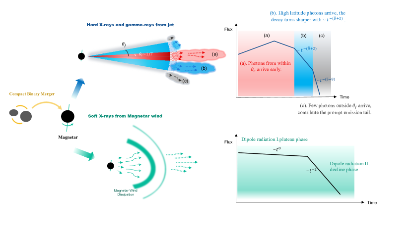
Figure 5: Schematic diagram of the two-component prompt emission of GRB 230307A. GRB 230307A is suggested to be powered by a millisecond magnetar resulting from a compact binary star merger. In such a scenario, the hard X-rays and gamma-ray are powered by a narrow jet. The early bright emission of the light curve is mainly contributed by photons from the jet within a cone of $\theta_{c}\sim 1/\Gamma$ at the emission radius $R_{\rm GRB}$ (Phase a). When the jet ceases, photons from higher-latitude parts arrive at later times, resulting in a decay in the light curve with a slope consistent with the curvature effect prediction (Phase b). After an achromatic break signaling the end of the curvature effect, the light curve decays with an even steeper slope. This enables us to estimate the jet opening angle, for the first time, during the prompt emission phase of a GRB. The tail of the prompt emission is possibly contributed by some weak emission from regions beyond the jet opening angle (Phase c). In contrast, the soft X-ray emission is powered by a presumably more isotropic magnetar wind. The light curve is consistent with prediction of the spin-down law with a plateau followed by a shallow decline.

We conduct a smoothly broken power law fit to the multi-wavelength flux light curves (Fig. 3a) and explain each of the segments using our schematic model depicted in Extended Data Fig. 5. The jet and magnetar-powered emission processes are displayed separately. The emission of the jet-dominated GRB component undergoes a rise followed by a general trend of decline contributed by photons within the jet core of $\theta_{c}=1/\Gamma$, where $\Gamma$ is the Lorentz factor. After the emitting shell terminates, the emission is contributed by photons from higher latitude regions with respect to the line of sight of the observer. The best-fit temporal slopes during this phase ($t_{\rm b2}$ – $t_{\rm b3}$ in Extended Date Table 4) are consistent with prediction of the high-latitude curvature effect relation $\hat{\alpha}(t)=2+\hat{\beta}(t)$ (Fig. 3c). Following the progressive decrease of the high-latitude emission, an achromatic break occurs, signaling the end of the curvature effect. This enables us to estimate the jet opening angle, for the first time, during the prompt emission phase of a GRB. Finally, the light curve drops with an even steeper slope, possibly contributed by some weak emission from regions beyond the opening angle of the jet that is likely to have no sharp edges. In contrast, the soft X-ray emission is powered by a presumably more isotropic magnetar wind. The light curve is dominated by the spin-down law with a plateau followed by a shallow decline.

0.9 Estimation of jet opening angle

The high-latitude emission effect is observed in the multi-wavelength flux light curves of GECAM, starting from the second break ($t_{\rm b2}$) and continuing until the third break ($t_{\rm b3}$), as depicted in Fig. 3 (see also Extended Data Table 4). The third break signifies the moment when photons from the outermost layer of the shell, with a radius $R_{\rm GRB}$, reach the observer. The duration of such tail emission can be described by the following relationship[79]:

$$\Delta t_{\rm b}=t_{\rm b3}-t_{\rm b2}=(1+z)\left(\frac{R_{\rm GRB}}{c}\right)\left(\frac{\theta_{j}^{2}}{2}\right),$$ (11)

where $\theta_{j}$ represents the half opening angle of the jet. By substituting $t_{\rm b3}=84.05$ s, $t_{\rm b2}=22.18$ s, and assuming a typical radius of $R_{\rm GRB}=10^{15}$ cm, we can calculate the opening angle of the jet as follows:

$$\theta_{j}=\sqrt{\frac{2c\Delta t_{\rm b}}{(1+z)R_{\rm GRB}}}\approx 3.4^{\circ}\left(\frac{\Delta t_{\rm b}}{62~{}\text{s}}\right)^{\frac{1}{2}}\left(\frac{R_{\rm GRB}}{10^{15}~{}\text{cm}}\right)^{-\frac{1}{2}}.$$ (12)

0.10 Host galaxy

We conducted a search for the host galaxy of GRB 230307A in various public galaxy catalogs and GCN circulars. We estimated the chance coincidence probability $P_{\rm cc}$[84] for the most promising candidates, which are listed below.

1. Large Magellanic Cloud (LMC): The LMC is the nearest and brightest galaxy to the Milky Way, located at a distance of 49 kpc. GRB 230307A is 8.15 degrees away from the center of the LMC, corresponding to a physical separation of 7 kpc, and it is situated on the edge of the Magellanic Bridge. The surface density of galaxies, typically used for estimating chance coincidence probabilities, is not applicable to the LMC due to its brightness. Instead, we consider a surface density of galaxies as bright as the LMC, which is $\sigma=1/41252.96$ deg^-2. Using a half-light radius of $r_{50}=2.2$ deg[85], we estimate the chance coincidence probability $P_{\rm cc}$ to be 0.006. However, the energy of the GRB is relatively low, around $\sim 9\times 10^{44}$ erg, which is inconsistent with any known transients. Additionally, it is unlikely for a transient with such low energy to produce gamma-ray photons. Therefore, we consider this scenario to be less likely.

2. Galaxy with a redshift of $z=3.87$: According to Ref.[45], there is a faint galaxy located 0.2 arcsec away from GRB 230307A with a redshift of $z=3.87$. We analyzed the JWST/NIRCam images using the official STScI JWST Calibration Pipeline version 1.9.0 and found the galaxy to be fainter than $28.5$ mag in the JWST/F070W bands and 27.4 mag in the JWST/F277W band. The estimated $P_{\rm cc}$ using the JWST/F277W magnitude is 0.034, while for the JWST/F070W band, it is estimated to be greater than 0.09. Since the F070W band is closer to the $r$ band, with which the galaxy brightness distribution is produced, the latter estimate is considered more reliable. However, the extremely high energy of the GRB and its inconsistency with known GRB transients in Fig. 2b and 2c make this scenario less favored.

3. Galaxy with a redshift of $z=0.065$[86, 14]: With the half-light radius and $r$ band magnitude from DESI Legacy Survey[87], the chance coincidence probability for this galaxy was estimated to be 0.11 (Table 1). Although not statistically significant, the redshift is more consistent with the physical properties of the GRB. Therefore, we consider this galaxy to be the most likely host. The offset of GRB 230307A from the host galaxy is 29.4", which is 36.6 kpc in redshift 0.065. As presented in Fig. 2d, the offset is consistent with those of type I GRB, and larger than type II GRBs.

Moreover, we explore other possible host galaxies in DESI Legacy Survey. For objects within 5 arcmin of GRB 230307A, we exclude stars with detected parallax in Gaia, and then calculate the chance coincidence probability with the half-light radius and $r$ band magnitude in the catalog. It turns out that the galaxy with a redshift of $z=0.065$ has the lowest $P_{\rm cc}$, while others have $P_{\rm cc}>0.2$ or more.

0.11 Magnetar dipole radiation

We fit the LEIA (0.5–4 keV) light curve of GRB 230307A in the prompt emission phase with both the smoothly broken power law model (Eq. 8) and the magnetar dipole radiation model.

Considering a millisecond magnetar with rigid rotation, it loses its rotational energy through both magnetic dipole radiation and quadrapole radiation [88, 1, 3, 7, 12], with

$$\dot{E}=I\Omega\dot{\Omega}=-\frac{B_{\rm p}^{2}R^{6}\Omega^{4}}{6c^{3}}-\frac{32GI^{2}\epsilon^{2}\Omega^{6}}{5c^{5}},$$ (13)

where $\dot{E}$ is the total spin-down rate, $\Omega=2\pi/P$ is the angular frequency and $\dot{\Omega}$ its time derivative, I is the moment of inertia ($=3.33\times 10^{45}$ $\rm g\,cm^{-2}$), $B_{\rm p}$ is the dipolar field strength at the magnetic poles on the NS surface, $R$ is the NS radius ($=1.2\times 10^{6}$ cm), and $\epsilon$ is the ellipticity of the NS ($=10^{-4}$). The electromagnetic emission is determined by the dipole spin-down luminosity $L_{\rm sd}$, i.e.,

$$L_{\rm X}(t)=\eta L_{\rm sd}=\frac{\eta B_{\rm p}^{2}R^{6}\Omega^{4}(t)}{6c^{3}},$$ (14)

where $\eta$ is the efficiency of converting the dipole spin-down luminosity to the X-ray luminosity. The X-ray luminosity is derived from the observation assuming isotropic emission. In a more realistic situation, the X-ray emission may not be isotropic, and a factor $f_{\rm b}$ (assumed to be 0.1) is introduced to account for this correction between the isotropic and true luminosity $L_{\rm X}$, i.e.,

$$L_{\rm iso}(t)=\frac{L_{\rm X}(t)}{f_{\rm b}}=\frac{\eta}{f_{\rm b}}\frac{B_{\rm p}^{2}R^{6}\Omega^{4}(t)}{6c^{3}}.$$ (15)

We model the unabsorbed luminosity light curves based on Eqs. 13 and 15. The fitting process is performed by using the Markov Chain Monte Carlo code emcee[74]. We employ $\chi^{2}$ as the statistical metric to evaluate the likelihood. The prior bounds for the free parameters ($\log(B_{\rm p}/{\rm G})$, $P_{0}/{\rm ms}$, $\log\eta$) are set to be $(15,17)$, $(1,5)$, and $(-3,-2)$, respectively. The first data point is excluded, as at this moment the light curve is still in the rising phase, and has not reached the main plateau emission yet. Theoretically it is also predicted that it takes seconds for the proto-neutron star to cool down[5]. The fitting results are shown in Extended Data Fig. 6.

Fast X-ray transients with light curves characteristic of spin-down magnetars have been identified previously in the afterglow of some short GRBs, as well as in a few events without associated GRB such as CDF-S XT2, which are thought to be of compact-star merger origin. We compare the X-ray luminosity light curve of GRB 230307A with internal plateaus in the X-ray afterglows of short GRBs with redshifts and in CDF-S XT2. The afterglow data are retrieved from the XRT lightcurve repository[89, 90] and corrected to the $0.5-4$ $\rm keV$ band assuming an absorbed power law spectrum. Such a correction is also made for the luminosity of CDF-S XT2, using power law indices $\Gamma_{1}=1.45$ and $\Gamma_{2}=2.67$ before and after the break time at 2.3 ks[11].

Data Availability

The processed data are presented in the tables and figures of the paper, which are available upon reasonable request. The authors point out that some data used in the paper are publicly available, whether through the UK Swift Science Data Centre website, JWST website, or GCN circulars.

Code Availability

Upon reasonable requests, the code (mostly in Python) used to produce the results and figures will be provided.

This work is supported by the National Key Research and Development Programs of China (2022YFF0711404, 2021YFA0718500, 2022SKA0130102, 2022SKA0130100). LEIA is a pathfinder of the Einstein Probe mission, which is supported by the Strategic Priority Program on Space Science of CAS (grant Nos. XDA15310000, XDA15052100). The GECAM (Huairou-1) mission is supported by the Strategic Priority Research Program on Space Science (Grant No. XDA15360000, XDA15360102, XDA15360300, XDA15052700) of CAS. We acknowledge the support by the National Natural Science Foundation of China (Grant Nos. 11833003, U2038105, 12121003, 12173055, 11922301, 12041306, 12103089, 12203071, 12103065, 12273042, 12173038, 12173056), the science research grants from the China Manned Space Project with NO.CMS-CSST-2021-B11, the Natural Science Foundation of Jiangsu Province (Grant No. BK20211000), International Partnership Program of Chinese Academy of Sciences for Grand Challenges (114332KYSB20210018), the Major Science and Technology Project of Qinghai Province (2019-ZJ-A10), the Youth Innovation Promotion Association of the Chinese Academy of Sciences, the Postgraduate Research & Practice Innovation Program of Jiangsu Province (KYCX23_0117), the Program for Innovative Talents, Entrepreneur in Jiangsu, and the International Partnership Program of Chinese Academy of Sciences (Grant No.113111KYSB20190020). We thank Y.-H. Yang, E. Troja, Y.-Z. Meng, Rahim Moradi, and Z.-G. Dai for helpful discussions.

H.S., S.-L.X. and B.-B.Z. initiated the study. H.S., B.-B.Z., B.Z., J.Y. and S.-L.X. coordinated the scientific investigations of the event. C.-W.W., W.-C.X., J.Y., Y.-H.I.Y., W.-J.T., J.-C.L., Y.-Q.Z., C.Zheng, C.C., S.X., S.-L.X., S.-X.Y. and X.-L.W. processed and analysed the GECAM data. S.-L.X. first noticed the extremely brightness of GRB 230307A from GECAM data. H.S., Y.Liu., H.-W.P. and D.-Y.L. processed and analysed the LEIA data. Y.Liu. first identified GRB 230307A in LEIA data. J.Y., C.-W.W., Y.-H.I.Y., W.-C.X. and Y.-Q. Z. performed the spectral fitting of GECAM data. W.-C.X. and J.-C.L. performed background analysis for GECAM-C. C.Zheng and Y.-Q.Z. performed calibration analysis for GECAM. J.-C.L. performed the data saturation assessment for GECAM. H.S., Y.Liu. and J.Y. performed the spectral fitting of LEIA data. C.Z., Z.-X.L., Y.Liu., H.-Q.C. and D.-H.Z. contributed to the calibration of LEIA data. J.Y. and C.-W. W. contributed the Amati relation and luminosity-lag relation. Y.-H.I.Y., J.Y. and C.-W.W. performed the $T_{90}$ calculation. J.Y. calculated the amplitude parameter. J.Y., W.-C.X., W.-J.T., Y.-H.I.Y. and S.X. calculated the spectral lag. W.-J.T., W.-C.X. and S.X. performed the minimum variability timescale calculation. J.Y. and C.-W.W. fitted the multi-wavelength flux light curves. J.Y. calculated the curvature effect. J.Y., H.S., Y.Liu., C.-W.W. W.-C.X. and Y.-Q.Z. contributed to the SED modeling. J.Y. performed the global fitting to the achromatic break. C.-W.W. and Z.Y. performed the calculation of jet opening angle. H.S. and J.Y. performed the theoretical modelling with the magnetar dipole radiation model. J.-W.H. contributed to the luminosity correction of the X-ray afterglows. Y. Li, L.H. and J.Y. contributed to the information about the host galaxy. Z.-X.L., C.Z., X.-J.S., S.L.S., X.-F.Z., Y.-H.Z., and W.Y. contributed to the development of the LEIA instrument. Y.Liu., H.-Q.C., C.J., W.-D.Z., D.-Y.L., J.-W.H., H.-Y.L., H.S., H.-W.P. and M.L. contributed to the development of LEIA data analysis tools and LEIA operations. Z.-H.A., X.-Q.L., W.-X.P., L.-M.S., X.-Y.W., F.Z., S.-J.Z., C.C., S.X. and S.-L.X. contributed to the development and operation of GECAM. B.Z. led the theoretical investigation of the event. H.S., J.Y., B.-B.Z., B.Z., W.Y., S.-L.X., S.-N.Z., Y. Liu contributed to the interpretation of the observations and the writing of the manuscript with contributions from all authors.

The authors declare that they have no competing financial interests.

Correspondence and requests for materials should be addressed to B.-B.Z.
(bbzhang@nju.edu.cn), S.-L.X. (xiongsl@ihep.ac.cn), Z.-X.L. (lingzhixing@nao.cas.cn) and B.Z.
(bing.zhang@unlv.edu).

\begin{overpic}[width=325.215pt]{Extended_Data_Figure_1a.pdf}\put(-4.0,75.0){\bf a}\end{overpic}
\begin{overpic}[width=173.44534pt]{Extended_Data_Figure_1b.pdf}\put(2.0,65.0){\bf b}\end{overpic}	\begin{overpic}[width=173.44534pt]{Extended_Data_Figure_1c.pdf}\put(2.0,65.0){\bf c}\end{overpic}

Figure 1: LEIA image and spectra. a, LEIA image. The blue square region represents the quarter of LEIA FoV adjacent to the source. The source with its XRT position denoted by the red cross is located outside of the nominal FoV of LEIA. Therefore only the cruciform arm structure of the point spread function (PSF) was observed, as shown by the brightening regions in the upper right corner. The black and purple solid lines around the source position shows the full PSF profile when the source is detected at this position (the data for generating the PSF profile is taken from on-ground calibration measurements). The regions encircled by red and orange dash-dotted lines are utilized in the extraction of the source and background photons, respectively. b, LEIA observed and model-predicted spectra in three time segments (LEIA S-I). c, Best-fit values of photon index $\Gamma_{\rm{ph}}$ and hydrogen column density $N_{\rm H}$ and 1$\sigma$, 2$\sigma$ confidence contours.

\begin{overpic}[width=138.76157pt]{Extended_Data_Figure_3a.pdf}\put(2.0,95.0){\bf a}\end{overpic}

\begin{overpic}[width=138.76157pt]{Extended_Data_Figure_3b.pdf}\put(2.0,95.0){\bf b}\end{overpic}

\begin{overpic}[width=130.08731pt]{Extended_Data_Figure_3c.pdf}\put(2.0,95.0){\bf c}\end{overpic}

Figure 3: The spectral fittings of LEIA and GECAM. a, The comparison between observed (points) and model-predicted (lines) count spectra and the residuals (pluses) based on the independent spectral fittings of LEIA S-III and GECAM S-III. b, The comparison between observed (points) and model-predicted (solid lines) count spectra and the residuals (pluses) based on the joint spectral fittings of LEIA S-III and GECAM S-III. For comparison, the model-predicted count spectra based on the independent spectral fittings of LEIA S-III are represented with dashed lines. c, The SEDs (solid lines) derived from the joint spectral fittings of LEIA S-III and GECAM S-III. For comparison, the SEDs derived from the independent spectral fittings of LEIA S-III are represented with unfilled dashed butterfly-shaped symbols. All error bars and shaded areas represent 1$\sigma$ uncertainties.

\begin{overpic}[width=216.81pt]{Extended_Data_Figure_6a.pdf}\put(2.0,95.0){\bf a}\end{overpic}

\begin{overpic}[width=216.81pt]{Extended_Data_Figure_6b.pdf}\put(2.0,95.0){\bf b}\end{overpic}

Figure 6: Corner plots of the posterior probability distributions of the parameters for the fit of the X-ray light curve (0.5–4 keV). a, Fit with the smoothly broken power law model. b, Fit with the magnetar dipole radiation model.

Table 1: Spectral fitting results and corresponding fitting statistics for LEIA S-II spectra. All errors represent the 1$\sigma$ uncertainties.

$t_{1}$	$t_{2}$	$\Gamma_{\rm ph}$	$norm$	CSTAT/d.o.f
(s)	(s)		(${\rm photons~{}cm^{-2}~{}s^{-1}~{}keV^{-1}}$)
$0$	$6$	$1.00_{-0.35}^{+0.36}$	$32.15_{-5.37}^{+6.06}$	$7.71/6$
$6$	$9$	$1.17_{-0.36}^{+0.37}$	$78.24_{-14.49}^{+16.99}$	$15.76/7$
$9$	$13$	$1.44_{-0.28}^{+0.29}$	$74.37_{-10.02}^{+11.12}$	$9.75/9$
$13$	$17$	$1.02_{-0.24}^{+0.24}$	$56.38_{-7.87}^{+8.58}$	$3.09/9$
$17$	$21$	$0.98_{-0.29}^{+0.30}$	$48.83_{-8.49}^{+9.71}$	$9.97/7$
$21$	$25$	$1.39_{-0.33}^{+0.33}$	$61.22_{-9.34}^{+10.51}$	$9.89/7$
$25$	$29$	$1.80_{-0.32}^{+0.33}$	$66.51_{-9.10}^{+10.03}$	$7.82/6$
$29$	$34$	$1.58_{-0.29}^{+0.30}$	$56.14_{-7.27}^{+7.96}$	$5.15/8$
$34$	$39$	$1.31_{-0.26}^{+0.27}$	$53.29_{-7.41}^{+8.23}$	$1.84/9$
$39$	$45$	$1.54_{-0.32}^{+0.34}$	$45.34_{-6.21}^{+6.88}$	$6.49/8$
$45$	$50$	$2.08_{-0.39}^{+0.40}$	$59.91_{-8.45}^{+9.15}$	$7.19/7$
$50$	$55$	$1.30_{-0.26}^{+0.26}$	$51.96_{-7.58}^{+7.69}$	$18.33/8$
$55$	$61$	$1.78_{-0.38}^{+0.39}$	$46.8_{-7.27}^{+8.17}$	$2.96/6$
$61$	$68$	$1.39_{-0.27}^{+0.28}$	$39.47_{-5.49}^{+5.98}$	$10.27/9$
$68$	$76$	$1.25_{-0.43}^{+0.46}$	$28.52_{-5.76}^{+6.63}$	$12.49/7$
$76$	$84$	$1.29_{-0.30}^{+0.30}$	$27.78_{-4.11}^{+4.51}$	$4.88/7$
$84$	$92$	$1.49_{-0.31}^{+0.31}$	$32.41_{-4.43}^{+4.89}$	$4.19/7$
$92$	$103$	$1.39_{-0.32}^{+0.33}$	$21.31_{-2.96}^{+3.27}$	$3.89/7$
$103$	$116$	$2.01_{-0.36}^{+0.37}$	$21.52_{-2.92}^{+3.17}$	$4.17/7$
$116$	$131$	$2.13_{-0.33}^{+0.35}$	$19.01_{-2.56}^{+2.79}$	$5.64/7$
$131$	$153$	$2.10_{-0.41}^{+0.43}$	$15.39_{-2.11}^{+2.33}$	$1.87/7$
$153$	$187$	$2.36_{-0.37}^{+0.39}$	$9.23_{-1.11}^{+1.20}$	$8.13/8$
$187$	$266$	$3.06_{-0.35}^{+0.36}$	$5.20_{-0.56}^{+0.59}$	$7.76/10$

In cases where the 1$\sigma$ lower limit of $\alpha$ falls below $-2$, we use cutoff energy as a substitute for peak energy.

Table 2: Spectral fitting results and corresponding fitting statistics for GECAM S-I and S-II spectra. All errors represent the 1$\sigma$ uncertainties.

$t_{1}$	$t_{2}$	$\alpha$	${\rm log}E_{\rm p}$	${\rm log}A$	PGSTAT/d.o.f
(s)	(s)		(${\rm keV}$)	(${\rm photons~{}cm^{-2}~{}s^{-1}~{}keV^{-1}}$)
$0$	$140$	$-1.198_{-0.002}^{+0.003}$	$3.098_{-0.006}^{+0.005}$	$-0.697_{-0.001}^{+0.001}$	$2127.85/662$
$0.000$	$0.700$	$-0.93_{-0.07}^{+0.05}$	$2.13_{-0.02}^{+0.02}$	$-0.03_{-0.04}^{+0.03}$	$468.69/662$
$0.700$	$1.000$	$-0.43_{-0.04}^{+0.05}$	$2.72_{-0.03}^{+0.03}$	$0.07_{-0.02}^{+0.02}$	$448.21/662$
$1.000$	$1.400$	$-0.62_{-0.04}^{+0.04}$	$2.66_{-0.02}^{+0.03}$	$0.03_{-0.02}^{+0.01}$	$448.30/662$
$1.400$	$1.600$	$-0.39_{-0.03}^{+0.03}$	$2.99_{-0.02}^{+0.02}$	$0.13_{-0.01}^{+0.01}$	$561.77/662$
$1.600$	$1.800$	$-0.40_{-0.04}^{+0.03}$	$3.10_{-0.02}^{+0.02}$	$0.10_{-0.01}^{+0.01}$	$580.31/662$
$1.800$	$2.000$	$-0.26_{-0.03}^{+0.03}$	$3.10_{-0.02}^{+0.02}$	$0.11_{-0.01}^{+0.01}$	$647.78/662$
$2.000$	$2.300$	$-0.33_{-0.03}^{+0.03}$	$2.90_{-0.02}^{+0.02}$	$0.11_{-0.01}^{+0.01}$	$561.17/662$
$2.300$	$2.700$	$-0.43_{-0.03}^{+0.03}$	$2.86_{-0.02}^{+0.02}$	$0.08_{-0.01}^{+0.01}$	$603.89/662$
$2.700$	$3.200$	$-0.68_{-0.03}^{+0.03}$	$2.81_{-0.03}^{+0.02}$	$-0.02_{-0.01}^{+0.01}$	$612.16/662$
$3.200$	$3.400$	$-0.40_{-0.02}^{+0.03}$	$3.09_{-0.02}^{+0.01}$	$0.29_{-0.01}^{+0.01}$	$614.24/662$
$3.400$	$3.600$	$-0.42_{-0.03}^{+0.03}$	$3.05_{-0.02}^{+0.02}$	$0.16_{-0.01}^{+0.01}$	$592.26/662$
$3.600$	$4.000$	$-0.56_{-0.02}^{+0.03}$	$2.81_{-0.02}^{+0.02}$	$0.06_{-0.01}^{+0.01}$	$536.76/662$
$4.000$	$4.300$	$-0.62_{-0.03}^{+0.03}$	$3.02_{-0.02}^{+0.02}$	$0.00_{-0.01}^{+0.01}$	$588.84/662$
$4.300$	$4.700$	$-0.67_{-0.03}^{+0.03}$	$2.87_{-0.02}^{+0.02}$	$0.06_{-0.01}^{+0.01}$	$540.47/662$
$4.700$	$4.900$	$-0.56_{-0.03}^{+0.03}$	$2.97_{-0.02}^{+0.02}$	$0.22_{-0.01}^{+0.01}$	$559.74/662$
$4.900$	$5.035$	$-0.59_{-0.04}^{+0.02}$	$2.85_{-0.02}^{+0.03}$	$0.32_{-0.01}^{+0.01}$	$515.88/662$
$5.035$	$5.200$	$-0.70_{-0.02}^{+0.02}$	$3.03_{-0.02}^{+0.02}$	$0.30_{-0.01}^{+0.01}$	$568.22/662$
$5.200$	$5.400$	$-0.62_{-0.03}^{+0.02}$	$2.96_{-0.02}^{+0.02}$	$0.33_{-0.01}^{+0.01}$	$535.36/662$
$5.400$	$5.700$	$-0.73_{-0.02}^{+0.02}$	$2.98_{-0.02}^{+0.02}$	$0.19_{-0.01}^{+0.01}$	$546.81/662$
$5.700$	$5.830$	$-0.60_{-0.03}^{+0.03}$	$3.08_{-0.02}^{+0.02}$	$0.25_{-0.01}^{+0.01}$	$552.10/662$
$5.830$	$5.940$	$-0.45_{-0.04}^{+0.04}$	$3.10_{-0.02}^{+0.02}$	$0.30_{-0.01}^{+0.01}$	$598.12/662$
$5.940$	$6.050$	$-0.51_{-0.03}^{+0.03}$	$3.03_{-0.02}^{+0.02}$	$0.35_{-0.01}^{+0.01}$	$543.25/662$
$6.050$	$6.200$	$-0.53_{-0.03}^{+0.03}$	$3.01_{-0.02}^{+0.02}$	$0.36_{-0.01}^{+0.01}$	$630.36/662$
$6.200$	$6.300$	$-0.49_{-0.03}^{+0.03}$	$3.06_{-0.02}^{+0.02}$	$0.43_{-0.01}^{+0.01}$	$612.34/662$
$6.300$	$6.415$	$-0.55_{-0.03}^{+0.03}$	$3.04_{-0.02}^{+0.02}$	$0.34_{-0.01}^{+0.01}$	$555.81/662$
$6.415$	$6.600$	$-0.62_{-0.02}^{+0.03}$	$3.11_{-0.02}^{+0.02}$	$0.29_{-0.01}^{+0.01}$	$696.62/662$
$6.600$	$6.700$	$-0.48_{-0.04}^{+0.03}$	$3.06_{-0.02}^{+0.02}$	$0.38_{-0.01}^{+0.01}$	$579.16/662$
$6.700$	$6.900$	$-0.58_{-0.02}^{+0.02}$	$2.97_{-0.02}^{+0.02}$	$0.34_{-0.01}^{+0.01}$	$583.81/662$
$6.900$	$7.200$	$-0.77_{-0.03}^{+0.03}$	$2.83_{-0.02}^{+0.03}$	$0.10_{-0.01}^{+0.01}$	$521.23/662$
$7.200$	$7.400$	$-0.69_{-0.03}^{+0.03}$	$2.89_{-0.02}^{+0.03}$	$0.22_{-0.01}^{+0.01}$	$583.81/662$
$7.400$	$7.700$	$-0.84_{-0.04}^{+0.03}$	$2.69_{-0.03}^{+0.03}$	$0.15_{-0.02}^{+0.02}$	$523.88/662$
$7.700$	$7.900$	$-0.85_{-0.03}^{+0.03}$	$2.81_{-0.03}^{+0.03}$	$0.22_{-0.01}^{+0.01}$	$571.07/662$
$7.900$	$8.100$	$-0.73_{-0.02}^{+0.02}$	$3.00_{-0.02}^{+0.02}$	$0.25_{-0.01}^{+0.01}$	$596.95/662$
$8.100$	$8.300$	$-0.70_{-0.02}^{+0.03}$	$3.07_{-0.02}^{+0.02}$	$0.27_{-0.01}^{+0.01}$	$581.17/662$
$8.300$	$8.445$	$-0.71_{-0.03}^{+0.03}$	$3.07_{-0.03}^{+0.03}$	$0.24_{-0.01}^{+0.01}$	$590.15/662$
$8.445$	$8.600$	$-0.71_{-0.02}^{+0.03}$	$3.14_{-0.03}^{+0.02}$	$0.27_{-0.01}^{+0.01}$	$596.36/662$
$8.600$	$8.900$	$-0.70_{-0.02}^{+0.03}$	$2.89_{-0.02}^{+0.02}$	$0.20_{-0.01}^{+0.01}$	$583.91/662$
$8.900$	$9.100$	$-0.73_{-0.03}^{+0.03}$	$2.90_{-0.03}^{+0.03}$	$0.14_{-0.01}^{+0.01}$	$509.65/662$
$9.100$	$9.315$	$-0.80_{-0.04}^{+0.03}$	$2.83_{-0.03}^{+0.03}$	$0.14_{-0.01}^{+0.01}$	$520.01/662$
$9.315$	$9.500$	$-0.68_{-0.03}^{+0.03}$	$2.82_{-0.02}^{+0.02}$	$0.29_{-0.01}^{+0.01}$	$561.81/662$
$9.500$	$9.695$	$-0.86_{-0.03}^{+0.03}$	$3.01_{-0.03}^{+0.03}$	$0.14_{-0.01}^{+0.01}$	$612.53/662$
$9.695$	$10.000$	$-0.83_{-0.02}^{+0.02}$	$3.05_{-0.03}^{+0.03}$	$0.05_{-0.01}^{+0.01}$	$534.35/662$
$10.000$	$10.300$	$-0.74_{-0.02}^{+0.02}$	$3.04_{-0.02}^{+0.02}$	$0.20_{-0.01}^{+0.01}$	$638.45/662$
$10.300$	$10.500$	$-0.74_{-0.03}^{+0.03}$	$2.91_{-0.03}^{+0.03}$	$0.15_{-0.01}^{+0.01}$	$550.87/662$
$10.500$	$10.700$	$-0.77_{-0.02}^{+0.03}$	$2.89_{-0.03}^{+0.02}$	$0.23_{-0.01}^{+0.01}$	$606.41/662$
$10.700$	$10.905$	$-0.77_{-0.03}^{+0.04}$	$2.83_{-0.03}^{+0.03}$	$0.15_{-0.01}^{+0.01}$	$481.37/662$
$10.905$	$11.200$	$-0.83_{-0.04}^{+0.03}$	$2.68_{-0.03}^{+0.04}$	$0.14_{-0.02}^{+0.02}$	$569.07/662$
$11.200$	$11.400$	$-0.81_{-0.03}^{+0.03}$	$2.80_{-0.03}^{+0.03}$	$0.21_{-0.01}^{+0.01}$	$535.59/662$
$11.400$	$11.700$	$-0.93_{-0.03}^{+0.04}$	$2.65_{-0.04}^{+0.04}$	$0.12_{-0.02}^{+0.02}$	$550.06/662$
$11.700$	$12.000$	$-1.01_{-0.02}^{+0.02}$	$2.88_{-0.03}^{+0.03}$	$0.11_{-0.01}^{+0.01}$	$611.71/662$
$12.000$	$12.245$	$-0.97_{-0.03}^{+0.03}$	$2.84_{-0.04}^{+0.03}$	$0.07_{-0.01}^{+0.02}$	$518.67/662$
$12.245$	$12.600$	$-0.98_{-0.02}^{+0.02}$	$2.88_{-0.04}^{+0.03}$	$0.08_{-0.01}^{+0.01}$	$581.00/662$
$12.600$	$12.900$	$-0.92_{-0.03}^{+0.02}$	$2.84_{-0.03}^{+0.03}$	$0.15_{-0.01}^{+0.01}$	$651.58/662$
$12.900$	$13.100$	$-0.91_{-0.03}^{+0.03}$	$2.72_{-0.03}^{+0.03}$	$0.32_{-0.01}^{+0.01}$	$561.25/662$
$13.100$	$13.300$	$-0.94_{-0.03}^{+0.03}$	$2.79_{-0.04}^{+0.03}$	$0.27_{-0.01}^{+0.01}$	$562.85/662$
$13.300$	$13.505$	$-1.05_{-0.03}^{+0.04}$	$2.80_{-0.05}^{+0.04}$	$0.15_{-0.01}^{+0.02}$	$529.89/662$
$13.505$	$14.000$	$-1.05_{-0.03}^{+0.03}$	$2.67_{-0.04}^{+0.03}$	$0.04_{-0.01}^{+0.01}$	$578.25/662$
$14.000$	$14.400$	$-1.08_{-0.02}^{+0.03}$	$2.85_{-0.03}^{+0.03}$	$0.08_{-0.01}^{+0.01}$	$660.04/662$
$14.400$	$14.900$	$-1.02_{-0.04}^{+0.03}$	$2.41_{-0.02}^{+0.03}$	$0.13_{-0.02}^{+0.02}$	$530.75/662$
$14.900$	$15.300$	$-1.07_{-0.02}^{+0.04}$	$2.66_{-0.04}^{+0.03}$	$0.12_{-0.01}^{+0.02}$	$497.61/662$
$15.300$	$15.900$	$-1.21_{-0.02}^{+0.03}$	$2.67_{-0.04}^{+0.05}$	$-0.01_{-0.01}^{+0.01}$	$594.82/662$
$15.900$	$16.600$	$-1.17_{-0.02}^{+0.02}$	$2.83_{-0.03}^{+0.04}$	$-0.10_{-0.01}^{+0.01}$	$534.37/662$
$16.600$	$17.400$	$-1.25_{-0.03}^{+0.03}$	$2.57_{-0.04}^{+0.04}$	$-0.14_{-0.02}^{+0.01}$	$482.42/662$
$17.400$	$18.600$	$-1.43_{-0.04}^{+0.03}$	$2.35_{-0.04}^{+0.06}$	$-0.50_{-0.03}^{+0.02}$	$498.41/662$
$18.600$	$19.300$	$-1.30_{-0.04}^{+0.04}$	$2.35_{-0.04}^{+0.05}$	$-0.24_{-0.03}^{+0.02}$	$522.11/662$
$19.300$	$19.900$	$-1.15_{-0.04}^{+0.03}$	$2.45_{-0.03}^{+0.04}$	$-0.03_{-0.02}^{+0.02}$	$543.22/662$
$19.900$	$20.400$	$-1.22_{-0.03}^{+0.04}$	$2.65_{-0.05}^{+0.05}$	$-0.05_{-0.01}^{+0.02}$	$584.43/662$
$20.400$	$21.100$	$-1.21_{-0.03}^{+0.02}$	$2.68_{-0.03}^{+0.05}$	$-0.19_{-0.02}^{+0.01}$	$533.13/662$
$21.100$	$21.500$	$-1.16_{-0.03}^{+0.03}$	$2.69_{-0.05}^{+0.05}$	$-0.05_{-0.02}^{+0.02}$	$509.46/662$
$21.500$	$22.100$	$-1.20_{-0.03}^{+0.03}$	$2.55_{-0.04}^{+0.05}$	$-0.12_{-0.02}^{+0.02}$	$500.03/662$
$22.100$	$22.900$	$-1.25_{-0.03}^{+0.04}$	$2.47_{-0.04}^{+0.04}$	$-0.21_{-0.02}^{+0.02}$	$561.92/662$
$22.900$	$23.500$	$-1.08_{-0.05}^{+0.05}$	$2.25_{-0.02}^{+0.03}$	$-0.09_{-0.03}^{+0.03}$	$445.08/662$
$23.500$	$24.300$	$-1.30_{-0.04}^{+0.03}$	$2.38_{-0.03}^{+0.05}$	$-0.16_{-0.02}^{+0.02}$	$619.11/662$
$24.300$	$25.000$	$-1.30_{-0.03}^{+0.03}$	$2.56_{-0.04}^{+0.06}$	$-0.19_{-0.02}^{+0.02}$	$450.48/662$
$25.000$	$25.600$	$-1.19_{-0.03}^{+0.05}$	$2.25_{-0.03}^{+0.02}$	$-0.04_{-0.02}^{+0.03}$	$443.31/662$
$25.600$	$26.300$	$-1.38_{-0.03}^{+0.05}$	$2.20_{-0.03}^{+0.03}$	$-0.19_{-0.02}^{+0.03}$	$417.92/662$
$26.300$	$27.800$	$-1.66_{-0.03}^{+0.03}$	$2.19_{-0.03}^{+0.05}$	$-0.41_{-0.02}^{+0.02}$	$525.19/662$
$27.800$	$28.500$	$-1.50_{-0.04}^{+0.03}$	$2.49_{-0.05}^{+0.08}$	$-0.26_{-0.02}^{+0.02}$	$572.05/662$
$28.500$	$29.700$	$-1.56_{-0.03}^{+0.03}$	$2.51_{-0.06}^{+0.07}$	$-0.55_{-0.02}^{+0.02}$	$512.87/662$
$29.700$	$32.000$	$-1.66_{-0.03}^{+0.03}$	$2.40_{-0.05}^{+0.08}$	$-0.69_{-0.02}^{+0.02}$	$509.14/662$
$32.000$	$33.300$	$-1.78_{-0.05}^{+0.05}$	$2.03_{-0.05}^{+0.07}$	$-0.74_{-0.03}^{+0.03}$	$446.42/662$
$33.300$	$34.015$	$-1.73_{-0.05}^{+0.04}$	$2.24_{-0.08}^{+0.10}$	$-0.71_{-0.03}^{+0.03}$	$485.83/662$
$34.015$	$34.700$	$-1.63_{-0.05}^{+0.05}$	$2.21_{-0.05}^{+0.09}$	$-0.63_{-0.04}^{+0.03}$	$460.20/662$
$34.700$	$35.600$	$-1.63_{-0.04}^{+0.04}$	$2.23_{-0.05}^{+0.07}$	$-0.56_{-0.03}^{+0.03}$	$469.85/662$
$35.600$	$36.800$	$-1.56_{-0.05}^{+0.05}$	$2.05_{-0.03}^{+0.05}$	$-0.64_{-0.04}^{+0.03}$	$438.21/662$
$36.800$	$37.550$	$-1.63_{-0.06}^{+0.05}$	$2.07_{-0.04}^{+0.06}$	$-0.62_{-0.04}^{+0.03}$	$439.23/662$
$37.550$	$38.900$	$-1.62_{-0.06}^{+0.04}$	$2.19_{-0.04}^{+0.09}$	$-0.79_{-0.04}^{+0.02}$	$476.73/662$
$38.900$	$40.600$	$-1.81_{-0.05}^{+0.04}$	$2.17_{-0.08}^{+0.15}$	$-1.01_{-0.03}^{+0.03}$	$438.00/662$
$40.600$	$44.600$	$-1.91_{-0.05}^{+0.03}$	$1.76_{-0.13}^{+0.07}$	$-1.10_{-0.04}^{+0.02}$	$466.40/662$
$44.600$	$47.700$	$-1.84_{-0.05}^{+0.05}$	$1.94_{-0.06}^{+0.07}$	$-1.10_{-0.03}^{+0.03}$	$435.60/662$
$47.700$	$51.000$	$-1.75_{-0.06}^{+0.04}$	$2.14_{-0.05}^{+0.12}$	$-1.10_{-0.04}^{+0.03}$	$470.74/662$
$51.000$	$55.200$	$-1.83_{-0.06}^{+0.06}$	$1.70_{-0.08}^{+0.06}$	$-1.21_{-0.05}^{+0.04}$	$465.16/662$
$55.200$	$61.600$	$-1.95_{-0.02}^{+0.07}$	$1.32_{-0.19}^{+0.23}$	$-1.39_{-0.02}^{+0.05}$	$468.45/662$
$61.600$	$69.600$	$-1.94_{-0.08}^{+0.05}$	($2.69_{-0.13}^{+0.45}$)*	$-1.56_{-0.06}^{+0.04}$	$459.07/662$
$69.600$	$80.000$	$-1.94_{-0.14}^{+0.10}$	($2.48_{-0.19}^{+0.55}$)	$-1.80_{-0.11}^{+0.08}$	$455.71/662$
$80.000$	$90.000$	$-2.01_{-0.12}^{+0.09}$	($2.69_{-0.22}^{+0.89}$)	$-1.92_{-0.09}^{+0.06}$	$453.34/662$
$90.000$	$100.000$	$-2.17_{-0.22}^{+0.07}$	unconstrained	$-2.23_{-0.16}^{+0.04}$	$397.65/662$
$100.000$	$115.000$	$-2.16_{-0.39}^{+0.14}$	unconstrained	$-2.53_{-0.32}^{+0.09}$	$336.77/662$
$115.000$	$140.000$	$-2.56_{-0.53}^{+0.22}$	unconstrained	$-3.01_{-0.40}^{+0.12}$	$264.86/662$

Table 3: Spectral fitting results and corresponding fitting statistics for LEIA S-III and GECAM S-III spectra. All errors represent the 1$\sigma$ uncertainties.

Time	$\alpha_{1}$	$\alpha_{2}$	${\rm log}E_{\rm b}$	${\rm log}E_{\rm p}$	${\rm log}A$	STAT/d.o.f.
(s)			(${\rm keV}$)	(${\rm keV}$)	(${\rm photons~{}cm^{-2}~{}s^{-1}~{}keV^{-1}}$)
LEIA S-III:
(1) 0–6	–	$-1.19_{-0.26}^{+0.26}$	–	–	$-0.87_{-0.49}^{+0.48}$	$10.80/7$
(2) 6–9	–	$-1.29_{-0.27}^{+0.24}$	–	–	$-0.71_{-0.50}^{+0.43}$	$26.46/9$
(3) 9–13	–	$-1.40_{-0.25}^{+0.23}$	–	–	$-0.93_{-0.47}^{+0.43}$	$9.47/11$
(4) 13–18	–	$-1.13_{-0.23}^{+0.19}$	–	–	$-0.50_{-0.43}^{+0.35}$	$8.74/12$
(5) 18–25	–	$-1.39_{-0.21}^{+0.20}$	–	–	$-1.02_{-0.39}^{+0.37}$	$17.52/14$
(6) 25–35	–	$-1.53_{-0.16}^{+0.15}$	–	–	$-1.29_{-0.32}^{+0.28}$	$23.08/21$
(7) 35–50	–	$-1.70_{-0.17}^{+0.16}$	–	–	$-1.68_{-0.32}^{+0.30}$	$14.66/26$
(8) 50–75	–	$-1.42_{-0.12}^{+0.12}$	–	–	$-1.23_{-0.22}^{+0.21}$	$31.71/36$
(9) 75–100	–	$-1.61_{-0.16}^{+0.16}$	–	–	$-1.73_{-0.30}^{+0.30}$	$27.23/26$
(10) 100–140	–	$-1.90_{-0.17}^{+0.16}$	–	–	$-2.49_{-0.33}^{+0.31}$	$13.02/25$
GECAM S-III:
(1) 0–6	–	$-0.66_{-0.01}^{+0.01}$	–	$3.047_{-0.004}^{+0.005}$	$0.083_{-0.002}^{+0.001}$	$996.60/662$
(2) 6–9	–	$-0.72_{-0.01}^{+0.01}$	–	$3.069_{-0.006}^{+0.005}$	$0.245_{-0.002}^{+0.002}$	$994.78/662$
(3) 9–13	–	$-0.90_{-0.01}^{+0.01}$	–	$2.98_{-0.01}^{+0.01}$	$0.152_{-0.002}^{+0.003}$	$1123.77/662$
(4) 13–18	$-0.46_{-0.09}^{+0.11}$	$-1.33_{-0.01}^{+0.01}$	$1.77_{-0.03}^{+0.03}$	$2.92_{-0.01}^{+0.02}$	$1.48_{-0.12}^{+0.10}$	$731.11/660$
(5) 18–25	$-0.75_{-0.08}^{+0.07}$	$-1.50_{-0.02}^{+0.01}$	$1.78_{-0.03}^{+0.03}$	$2.83_{-0.02}^{+0.03}$	$1.77_{-0.08}^{+0.09}$	$697.15/660$
(6) 25–35	$-1.02_{-0.10}^{+0.13}$	$-1.77_{-0.02}^{+0.01}$	$1.67_{-0.03}^{+0.03}$	$2.59_{-0.04}^{+0.06}$	$2.09_{-0.13}^{+0.10}$	$685.42/660$
(7) 35–50	–	$-1.79_{-0.02}^{+0.02}$	–	$2.20_{-0.03}^{+0.04}$	$-0.92_{-0.01}^{+0.01}$	$592.47/662$
(8) 50–75	–	$-1.91_{-0.03}^{+0.03}$	–	$1.66_{-0.07}^{+0.08}$	$-1.40_{-0.03}^{+0.02}$	$606.06/662$
(9) 75–100	–	$-2.06_{-0.12}^{+0.05}$	–	$2.64_{-0.13}^{+0.88}$	$-1.96_{-0.09}^{+0.04}$	$516.62/662$
(10) 100–140	–	$-2.39_{-0.24}^{+0.26}$	–	$2.50_{-0.45}^{+1.13}$	$-2.76_{-0.18}^{+0.20}$	$232.39/662$
LEIA S-III & GECAM S-III:
(1) 0–6	–	$-0.66_{-0.01}^{+0.01}$	–	$3.046_{-0.004}^{+0.006}$	$0.083_{-0.002}^{+0.001}$	$1011.62/671$
(2) 6–9	–	$-0.72_{-0.01}^{+0.01}$	–	$3.069_{-0.005}^{+0.006}$	$0.245_{-0.002}^{+0.001}$	$1028.06/673$
(3) 9–13	–	$-0.89_{-0.01}^{+0.01}$	–	$2.97_{-0.01}^{+0.01}$	$0.153_{-0.002}^{+0.002}$	$1155.65/675$
(4) 13–18	$-0.61_{-0.04}^{+0.03}$	$-1.34_{-0.01}^{+0.02}$	$1.82_{-0.02}^{+0.02}$	$2.93_{-0.02}^{+0.01}$	$1.65_{-0.04}^{+0.04}$	$749.17/674$
(5) 18–25	$-0.68_{-0.03}^{+0.04}$	$-1.50_{-0.02}^{+0.01}$	$1.76_{-0.01}^{+0.02}$	$2.83_{-0.02}^{+0.03}$	$1.69_{-0.04}^{+0.03}$	$731.98/676$
(6) 25–35	$-0.62_{-0.02}^{+0.05}$	$-1.76_{-0.02}^{+0.02}$	$1.59_{-0.02}^{+0.02}$	$2.59_{-0.05}^{+0.04}$	$1.68_{-0.05}^{+0.02}$	$751.70/683$
(7) 35–50	$-0.71_{-0.05}^{+0.04}$	$-1.82_{-0.04}^{+0.01}$	$1.41_{-0.02}^{+0.05}$	$2.21_{-0.04}^{+0.06}$	$1.62_{-0.03}^{+0.03}$	$643.45/688$
(8) 50–75	$-0.97_{-0.06}^{+0.06}$	$-1.89_{-0.06}^{+0.01}$	$1.31_{-0.04}^{+0.06}$	$1.69_{-0.16}^{+0.03}$	$1.58_{-0.03}^{+0.03}$	$650.51/698$
(9) 75–100	–	$-1.53_{-0.03}^{+0.03}$	–	$1.61_{-0.03}^{+0.03}$	$-1.56_{-0.04}^{+0.04}$	$561.87/690$
(10) 100–140	–	$-1.77_{-0.09}^{+0.06}$	–	$1.15_{-0.07}^{+0.07}$	$-2.24_{-0.16}^{+0.10}$	$246.89/689$

Table 4: Smoothly broken power law fitting results to the flux light curves. All errors represent the 1$\sigma$ uncertainties.

Energy	$\hat{\alpha}_{1}$		$\hat{\alpha}_{2}$		$t_{\rm b}$			${\rm log}A$	$\chi^{2}$/d.o.f.
(keV)						(s)		(${\rm erg~{}cm^{-2}~{}s^{-1}}$)
LF: $0.5-4$	$0.40_{-0.06}^{+0.05}$		$2.33_{-0.15}^{+0.16}$		$79.90_{-5.78}^{+5.42}$			$-6.84_{-0.04}^{+0.04}$	$12.28/17$
Energy	$\hat{\alpha}_{1}$	$\hat{\alpha}_{2}$	$\hat{\alpha}_{3}$	$\hat{\alpha}_{4}$	$t_{\rm b1}$	$t_{\rm b2}$	$t_{\rm b3}$	${\rm log}A$	$\chi^{2}$/d.o.f.
(keV)					(s)	(s)	(s)	(${\rm erg~{}cm^{-2}~{}s^{-1}}$)
GF1: $15-30$	$-0.52_{-0.01}^{+0.01}$	$0.49_{-0.03}^{+0.03}$	$2.44_{-0.02}^{+0.02}$	$5.03_{-0.34}^{+0.34}$	$13.07_{-0.28}^{+0.28}$	$27.41_{-0.20}^{+0.20}$		$-5.488_{-0.003}^{+0.003}$
GF2: $30-100$	$-0.76_{-0.02}^{+0.02}$	$0.49_{-0.01}^{+0.01}$	$2.80_{-0.02}^{+0.02}$	$6.44_{-0.53}^{+0.55}$	$6.59_{-0.09}^{+0.09}$	$22.18_{-0.18}^{+0.16}$	$84.05_{-2.19}^{+1.66}$	$-4.763_{-0.002}^{+0.002}$	$33052.22/249$
GF3: $100-350$	$-0.41_{-0.01}^{+0.01}$	$1.19_{-0.01}^{+0.01}$	$3.42_{-0.02}^{+0.02}$	$7.72_{-1.16}^{+1.29}$	$6.67_{-0.04}^{+0.04}$	$20.47_{-0.13}^{+0.13}$		$-4.111_{-0.002}^{+0.002}$
GF4: $350-700$	$-0.31_{-0.01}^{+0.01}$	$1.84_{-0.02}^{+0.02}$	$4.14_{-0.08}^{+0.08}$	–	$6.97_{-0.04}^{+0.05}$	$19.69_{-0.32}^{+0.30}$	–	$-3.995_{-0.003}^{+0.003}$	$12010.95/85$
GF5: $700-2000$	$-0.17_{-0.03}^{+0.03}$	$2.98_{-0.11}^{+0.12}$	$4.59_{-0.17}^{+0.19}$	–	$7.48_{-0.14}^{+0.14}$	$17.92_{-1.14}^{+1.21}$	–	$-3.67_{-0.01}^{+0.01}$	$4674.73/85$

References

- [1] Usov, V. V. Millisecond pulsars with extremely strong magnetic fields as a cosmological source of -ray bursts. Nature 357, 472–474 (1992).
- [2] Dai, Z. G. & Lu, T. -Ray Bursts and Afterglows from Rotating Strange Stars and Neutron Stars. Phys. Rev. Lett. 81, 4301–4304 (1998).
- [3] Zhang, B. & Mészáros, P. Gamma-Ray Burst Afterglow with Continuous Energy Injection: Signature of a Highly Magnetized Millisecond Pulsar. ApJ 552, L35–L38 (2001).
- [4] Dai, Z. G., Wang, X. Y., Wu, X. F. & Zhang, B. X-ray Flares from Postmerger Millisecond Pulsars. Science 311, 1127–1129 (2006).
- [5] Metzger, B. D., Giannios, D., Thompson, T. A., Bucciantini, N. & Quataert, E. The protomagnetar model for gamma-ray bursts. MNRAS 413, 2031–2056 (2011).
- [6] Zhang, B. Early X-Ray and Optical Afterglow of Gravitational Wave Bursts from Mergers of Binary Neutron Stars. ApJ 763, L22 (2013).
- [7] Gao, H., Zhang, B. & Lü, H.-J. Constraints on binary neutron star merger product from short GRB observations. Phys. Rev. D 93, 044065 (2016).
- [8] Margalit, B. & Metzger, B. D. The Multi-messenger Matrix: The Future of Neutron Star Merger Constraints on the Nuclear Equation of State. ApJ 880, L15 (2019).
- [9] Rowlinson, A., O’Brien, P. T., Metzger, B. D., Tanvir, N. R. & Levan, A. J. Signatures of magnetar central engines in short GRB light curves. MNRAS 430, 1061–1087 (2013).
- [10] Lü, H.-J., Zhang, B., Lei, W.-H., Li, Y. & Lasky, P. D. The Millisecond Magnetar Central Engine in Short GRBs. ApJ 805, 89 (2015).
- [11] Xue, Y. Q. et al. A magnetar-powered X-ray transient as the aftermath of a binary neutron-star merger. Nature 568, 198–201 (2019).
- [12] Sun, H. et al. A Unified Binary Neutron Star Merger Magnetar Model for the Chandra X-Ray Transients CDF-S XT1 and XT2. ApJ 886, 129 (2019).
- [13] Ciolfi, R. Collimated outflows from long-lived binary neutron star merger remnants. MNRAS 495, L66–L70 (2020).
- [14] Levan, A. et al. JWST detection of heavy neutron capture elements in a compact object merger. arXiv e-prints arXiv:2307.02098 (2023).
- [15] Li, X. Q. et al. The technology for detection of gamma-ray burst with GECAM satellite. Radiation Detection Technology and Methods 6, 12–25 (2021).
- [16] Zhang, D. et al. The performance of SiPM-based gamma-ray detector (GRD) of GECAM-C. arXiv e-prints arXiv:2303.00537 (2023).
- [17] Xiong, S., Wang, C., Huang, Y. & Gecam Team. GRB 230307A: GECAM detection of an extremely bright burst. GRB Coordinates Network 33406, 1 (2023).
- [18] Fermi GBM Team. GRB 230307A: Fermi GBM Final Real-time Localization. GRB Coordinates Network 33405, 1 (2023).
- [19] An, Z.-H. et al. Insight-HXMT and GECAM-C observations of the brightest-of-all-time GRB 221009A. arXiv e-prints arXiv:2303.01203 (2023).
- [20] Yuan, W., Zhang, C., Chen, Y. & Ling, Z. The Einstein Probe Mission. In Handbook of X-ray and Gamma-ray Astrophysics, 86 (2022).
- [21] Zhang, C. et al. First Wide Field-of-view X-Ray Observations by a Lobster-eye Focusing Telescope in Orbit. ApJ 941, L2 (2022).
- [22] Ling, Z. X. et al. The Lobster Eye Imager for Astronomy Onboard the SATech-01 Satellite. arXiv e-prints arXiv:2305.14895 (2023).
- [23] Liu, M. J. et al. GRB 230307A: soft X-ray detection with LEIA. GRB Coordinates Network 33466, 1 (2023).
- [24] Yang, Y. H. in prep. (2023).
- [25] Zhang, B. et al. Discerning the Physical Origins of Cosmological Gamma-ray Bursts Based on Multiple Observational Criteria: The Cases of z = 6.7 GRB 080913, z = 8.2 GRB 090423, and Some Short/Hard GRBs. ApJ 703, 1696–1724 (2009).
- [26] Yang, J. et al. A long-duration gamma-ray burst with a peculiar origin. Nature 612, 232–235 (2022).
- [27] Golenetskii, S. V., Mazets, E. P., Aptekar, R. L. & Ilinskii, V. N. Correlation between luminosity and temperature in -ray burst sources. Nature 306, 451–453 (1983).
- [28] Kumar, P. & Panaitescu, A. Afterglow Emission from Naked Gamma-Ray Bursts. ApJ 541, L51–L54 (2000).
- [29] Wang, X.-G. et al. Gamma-Ray Burst Jet Breaks Revisited. ApJ 859, 160 (2018).
- [30] Oganesyan, G., Nava, L., Ghirlanda, G. & Celotti, A. Detection of Low-energy Breaks in Gamma-Ray Burst Prompt Emission Spectra. ApJ 846, 137 (2017).
- [31] Lu, W. & Quataert, E. Late-time accretion in neutron star mergers: Implications for short gamma-ray bursts and kilonovae. MNRAS 522, 5848–5861 (2023).
- [32] Lü, H.-J., Zhang, B., Liang, E.-W., Zhang, B.-B. & Sakamoto, T. The ‘amplitude’ parameter of gamma-ray bursts and its implications for GRB classification. MNRAS 442, 1922–1929 (2014).
- [33] Yin, Y.-H. I. et al. GRB 211211A-like Events and How Gravitational Waves May Tell Their Origin. arXiv e-prints arXiv:2304.06581 (2023).
- [34] Li, Y., Zhang, B. & Lü, H.-J. A Comparative Study of Long and Short GRBs. I. Overlapping Properties. ApJS 227, 7 (2016).

References

- [35] Fermi GBM Team. GRB 230307A: Fermi GBM detection of a very bright GRB. GRB Coordinates Network 33407, 1 (2023).
- [36] Fermi GBM Team. GRB 230307A: possibly the second highest GRB energy fluence ever identified. GRB Coordinates Network 33414, 1 (2023).
- [37] Svinkin, D. et al. Konus-Wind detection of GRB 230307A. GRB Coordinates Network 33427, 1 (2023).
- [38] Kozyrev, A. S. et al. Further improved IPN localization for GRB 230307A. GRB Coordinates Network 33461, 1 (2023).
- [39] Evans, P. A. & Swift Team. GRB 230307A: Tiled Swift observations. GRB Coordinates Network 33419, 1 (2023).
- [40] Burrows, D. N. et al. GRB 230307A: Swift-XRT afterglow detection. GRB Coordinates Network 33465, 1 (2023).
- [41] O’Connor, B. et al. GRB 230307A: Gemini-South Confirmation of the Optical Afterglow. GRB Coordinates Network 33447, 1 (2023).
- [42] Gillanders, J., O’Connor, B., Dichiara, S. & Troja, E. GRB 230307A: Continued Gemini-South observations confirm rapid optical fading. GRB Coordinates Network 33485, 1 (2023).
- [43] Levan, A. J. et al. GRB 230307A: JWST observations consistent with the presence of a kilonova. GRB Coordinates Network 33569, 1 (2023).
- [44] Levan, A. J. et al. GRB 230307A: JWST NIRSpec observations, possible higher redshift. GRB Coordinates Network 33580, 1 (2023).
- [45] Levan, A. J. et al. GRB 230307A: JWST second-epoch observations. GRB Coordinates Network 33747, 1 (2023).
- [46] Zhao, X.-Y. et al. The In-Flight Realtime Trigger and Localization Software of GECAM. arXiv e-prints arXiv:2112.05101 (2021).
- [47] Guo, S. et al. Integrated navigation and communication service for LEO satellites based on BDS-3 global short message communication. IEEE Access 11, 6623–6631 (2023).
- [48] An, Z. et al. The design and performance of GRD onboard the GECAM satellite. Radiation Detection Technology and Methods 6, 43–52 (2021).
- [49] Zheng, C. et al. Electron non-linear light yield of LaBr3 detector aboard GECAM. Nuclear Instruments and Methods in Physics Research A 1042, 167427 (2022).
- [50] Zheng, C. et al. Ground calibration of Gamma-Ray Detectors of GECAM-C. arXiv e-prints arXiv:2303.00687 (2023).
- [51] Zhang, Y.-Q. et al. Cross calibration of gamma-ray detectors (GRD) of GECAM-C. arXiv e-prints arXiv:2303.00698 (2023).
- [52] Fermi GBM Team. GRB 230307A: Bad Time Intervals for Fermi GBM data. GRB Coordinates Network 33551, 1 (2023).
- [53] Liu, Y. Q. et al. The SiPM Array Data Acquisition Algorithm Applied to the GECAM Satellite Payload. arXiv e-prints arXiv:2112.04786 (2021).
- [54] Golkhou, V. Z., Butler, N. R. & Littlejohns, O. M. The Energy Dependence of GRB Minimum Variability Timescales. ApJ 811, 93 (2015).
- [55] Camisasca, A. E. et al. GRB minimum variability timescale with Insight-HXMT and Swift. Implications for progenitor models, dissipation physics, and GRB classifications. A&A 671, A112 (2023).
- [56] Scargle, J. D., Norris, J. P., Jackson, B. & Chiang, J. Studies in Astronomical Time Series Analysis. VI. Bayesian Block Representations. ApJ 764, 167 (2013).
- [57] Yi, T., Liang, E., Qin, Y. & Lu, R. On the spectral lags of the short gamma-ray bursts. MNRAS 367, 1751–1756 (2006).
- [58] Bernardini, M. G. et al. Comparing the spectral lag of short and long gamma-ray bursts and its relation with the luminosity. MNRAS 446, 1129–1138 (2015).
- [59] Norris, J. P., Marani, G. F. & Bonnell, J. T. Connection between Energy-dependent Lags and Peak Luminosity in Gamma-Ray Bursts. ApJ 534, 248–257 (2000).
- [60] Ukwatta, T. N. et al. The lag-luminosity relation in the GRB source frame: an investigation with Swift BAT bursts. MNRAS 419, 614–623 (2012).
- [61] Zhang, B.-B. et al. Unusual Central Engine Activity in the Double Burst GRB 110709B. ApJ 748, 132 (2012).
- [62] Arnaud, K. A. XSPEC: The First Ten Years. In Jacoby, G. H. & Barnes, J. (eds.) Astronomical Data Analysis Software and Systems V, vol. 101 of Astronomical Society of the Pacific Conference Series, 17 (1996).
- [63] Cash, W. Parameter estimation in astronomy through application of the likelihood ratio. ApJ 228, 939–947 (1979).
- [64] HI4PI Collaboration et al. HI4PI: A full-sky H I survey based on EBHIS and GASS. A&A 594, A116 (2016).
- [65] Yang, J. et al. Synchrotron Radiation Dominates the Extremely Bright GRB 221009A. ApJ 947, L11 (2023).
- [66] Feroz, F. & Hobson, M. P. Multimodal nested sampling: an efficient and robust alternative to Markov Chain Monte Carlo methods for astronomical data analyses. MNRAS 384, 449–463 (2008).
- [67] Feroz, F., Hobson, M. P. & Bridges, M. MULTINEST: an efficient and robust Bayesian inference tool for cosmology and particle physics. MNRAS 398, 1601–1614 (2009).
- [68] Buchner, J. et al. X-ray spectral modelling of the AGN obscuring region in the CDFS: Bayesian model selection and catalogue. A&A 564, A125 (2014).
- [69] Feroz, F., Hobson, M. P., Cameron, E. & Pettitt, A. N. Importance Nested Sampling and the MultiNest Algorithm. The Open Journal of Astrophysics 2, 10 (2019).
- [70] Zheng, W. et al. Panchromatic Observations of the Textbook GRB 110205A: Constraining Physical Mechanisms of Prompt Emission and Afterglow. ApJ 751, 90 (2012).
- [71] Schwarz, G. Estimating the Dimension of a Model. Annals of Statistics 6, 461–464 (1978).
- [72] Amati, L. et al. Intrinsic spectra and energetics of BeppoSAX Gamma-Ray Bursts with known redshifts. A&A 390, 81–89 (2002).
- [73] Minaev, P. Y. & Pozanenko, A. S. The Ep,I-Eiso correlation: type I gamma-ray bursts and the new classification method. MNRAS 492, 1919–1936 (2020).
- [74] Foreman-Mackey, D., Hogg, D. W., Lang, D. & Goodman, J. emcee: The MCMC Hammer. PASP 125, 306 (2013).
- [75] Lelli, F., McGaugh, S. S., Schombert, J. M., Desmond, H. & Katz, H. The baryonic Tully-Fisher relation for different velocity definitions and implications for galaxy angular momentum. MNRAS 484, 3267–3278 (2019).
- [76] Ukwatta, T. N. et al. Spectral Lags and the Lag-Luminosity Relation: An Investigation with Swift BAT Gamma-ray Bursts. ApJ 711, 1073–1086 (2010).
- [77] Xiao, S. et al. A Robust Estimation of Lorentz Invariance Violation and Intrinsic Spectral Lag of Short Gamma-Ray Bursts. ApJ 924, L29 (2022).
- [78] Dermer, C. D. Curvature Effects in Gamma-Ray Burst Colliding Shells. ApJ 614, 284–292 (2004).
- [79] Zhang, B. et al. Physical Processes Shaping Gamma-Ray Burst X-Ray Afterglow Light Curves: Theoretical Implications from the Swift X-Ray Telescope Observations. ApJ 642, 354–370 (2006).
- [80] Liang, E. W. et al. Testing the Curvature Effect and Internal Origin of Gamma-Ray Burst Prompt Emissions and X-Ray Flares with Swift Data. ApJ 646, 351–357 (2006).
- [81] Uhm, Z. L. & Zhang, B. On the Curvature Effect of a Relativistic Spherical Shell. ApJ 808, 33 (2015).
- [82] Zhang, B.-B., Liang, E.-W. & Zhang, B. A Comprehensive Analysis of Swift XRT Data. I. Apparent Spectral Evolution of Gamma-Ray Burst X-Ray Tails. ApJ 666, 1002–1011 (2007).
- [83] Zhang, B.-B., Zhang, B., Liang, E.-W. & Wang, X.-Y. Curvature Effect of a Non-Power-Law Spectrum and Spectral Evolution of GRB X-Ray Tails. ApJ 690, L10–L13 (2009).
- [84] Bloom, J. S., Kulkarni, S. R. & Djorgovski, S. G. The Observed Offset Distribution of Gamma-Ray Bursts from Their Host Galaxies: A Robust Clue to the Nature of the Progenitors. AJ 123, 1111–1148 (2002).
- [85] Corwin, J., Harold G., Buta, R. J. & de Vaucouleurs, G. Corrections and additions to the Third Reference Catalogue of Bright Galaxies. AJ 108, 2128–2144 (1994).
- [86] Gillanders, J., O’Connor, B., Dichiara, S. & Troja, E. GRB 230307A: Continued Gemini-South observations confirm rapid optical fading. GRB Coordinates Network 33485, 1 (2023).
- [87] Dey, A. et al. Overview of the DESI Legacy Imaging Surveys. AJ 157, 168 (2019).
- [88] Shapiro, S. L. & Teukolsky, S. A. Black holes, white dwarfs and neutron stars. The physics of compact objects (1983).
- [89] Evans, P. A. et al. An online repository of Swift/XRT light curves of -ray bursts. A&A 469, 379–385 (2007).
- [90] Evans, P. A. et al. Methods and results of an automatic analysis of a complete sample of Swift-XRT observations of GRBs. MNRAS 397, 1177–1201 (2009).