Relationship between the gamma-ray burst pulse width and energy due to the Doppler effect of fireballs

Abstract

We study in details how the pulse width of gamma-ray bursts is related with energy under the assumption that the sources concerned are in the stage of fireballs. Due to the Doppler effect of fireballs, there exists a power law relationship between the two quantities within a limited range of frequency. The power law range and the power law index depend strongly on the observed peak energy $E_{p}$ as well as the rest frame radiation form, and the upper and lower limits of the power law range can be determined by $E_{p}$. It is found that, within the same power law range, the ratio of the $FWHM$ of the rising portion to that of the decaying phase of the pulses is also related with energy in the form of power laws. A platform-power-law-platform feature could be observed in the two relationships. In the case of an obvious softening of the rest frame spectrum, the two power law relationships also exist, but the feature would evolve to a peaked one. Predictions on the relationships in the energy range covering both the BATSE and Swift bands for a typical hard burst and a typical soft one are made. A sample of FRED (fast rise and exponential decay) pulse bursts shows that 27 out of the 28 sources belong to either the platform-power-law-platform feature class or the peaked feature group, suggesting that the effect concerned is indeed important for most of the sources of the sample. Among these bursts, many might undergo an obvious softening evolution of the rest frame spectrum.

1 Introduction

Owing to the large amount of energy observed, gamma-ray bursts (GRBs) were assumed to undergo a stage of fireballs which expand relativistically (see, e.g., Goodman 1986; Paczynski 1986). Relativistic bulk motion of the gamma-ray-emitting plasma would play a role in producing the observed phenomena of the sources (Krolik & Pier 1991). It was believed that the Doppler effect over the whole fireball surface (the so-called relativistic curvature effect) might be the key factor to account for the observed spectrum of the events (see, e.g., Meszaros & Rees 1998; Hailey et al. 1999; Qin 2002, 2003).

Some simple bursts with well-separated structure suggest that they may consist of fundamental units of radiation such as pulses, with some of them being seen to comprise a fast rise and an exponential decay (FRED) phases (see, e.g., Fishman et al. 1994). These FRED pulses could be well represented by flexible empirical or quasi-empirical functions (see e.g., Norris et al. 1996; Kocevski et al. 2003). Fitting the corresponding light curves with the empirical functions, many statistical properties of pulses were revealed. Light curves of GRB pulses were found to become narrower at higher energies (Fishman et al. 1992; Link, Epstein, & Priedhorsky 1993). Fenimore et al. (1995) showed that the average pulse width is related with energy by a power law with an index of about $-0.4$. This was confirmed by later studies (Fenimore et al. 1995; Norris et al. 1996, 2000; Costa 1998; Piro et al. 1998; Nemiroff 2000; Feroci et al. 2001; Crew et al. 2003).

In the past few years, many attempts of interpretation of light curves of GRBs have been made (see, e.g., Fenimore et al. 1996; Norris et al. 1996; Norris et al. 2000; Ryde & Petrosian 2002; Kocevski et al. 2003). It was suggested that the power law relationship could be attributed to synchrotron radiation (see Fenimore et al. 1995; Cohen et al. 1997; Piran 1999). Kazanas, Titarchuk, & Hua (1998) proposed that the relationship could be accounted for by synchrotron cooling (see also Chiang 1998; Dermer 1998; and Wang et al. 2000). Phenomena such as the hardness-intensity correlation and the FRED form of pulses were recently interpreted as signatures of the relativistic curvature effect (Fenimore et al. 1996; Ryde & Petrosian 2002; Kocevski et al. 2003; Qin et al. 2004, hereafter Paper I). It was suspected that the power law relationship might result from a relative projected speed or a relative beaming angle (Nemiroff 2000). Due to the feature of self-similarity across energy bands observed (see, e.g., Norris et al. 1996), it is likely that the observed difference between different channel light curves might mainly be due to the energy channels themselves. In other words, light curves of different energy channels might arise from the same mechanism (e.g., parameters of the rest frame spectrum and parameters of the expanding fireballs are the same for different energy ranges), differing only in the energy ranges involved.

We believe that, if different channel light curves of a burst can be accounted for by the same mechanism where, except the energy ranges concerned, no parameters are allowed to be different for different energy channels, then the mechanism must be the main cause of the observed difference. A natural mechanism that possesses this property might be the Doppler effect of the expanding fireball surface when a rest frame radiation form is assumed. Indeed, as shown in Paper I, the four channel light curves of GRB 951019 were found to be well fitted by a single formula derived when this effect was taken into account. In Paper I, the power law relationship between the pulse width and energy was interpreted as being mainly due to different active areas of the fireball surface corresponding to the majority of photons of these channels. However, how the width is related with energy remains unclear. Presented in the following is a detailed analysis on this issue and based on it predictions on the relationship over a wide band covering those of BATSE and Swift will be made.

This paper is organized as follows. In section 2, we investigate in a general manner how the width and the ratio of the rising width to the decaying width of GRB pulses are related with energy. Then we make predictions on the relationship over the BATSE and Swift bands for a typical hard and a typical soft bursts in section 3. In section 4, a sample containing 28 FRED pulse sources is employed to illustrate the relationship. A brief discussion and conclusions are presented in the last section.

2 General analysis on the relationship

Studies of the Doppler effect of the expanding fireball surface were presented by different authors, and based on these studies formulas applicable to various situations are available (see, e.g., Fenimore et al. 1996; Granot et al. 1999; Eriksen & Gron 2000; Dado et al. 2002a, 2002b; Ryde & Petrosian 2002; Kocevski et al. 2003; Paper I; Shen et al. 2005). Employed in the following is one of them suitable for studying the issue concerned above, where a highly symmetric and expanding fireball is concerned.

It can be verified that the expected flux of a fireball expanding with a Lorentz factor $\Gamma>1$ can be determined by (for a detailed derivation for this form of formula one can refer to Paper I)

$$f_{\nu}(\tau)=\frac{2\pi R_{c}^{2}}{D^{2}\Gamma^{3}(1-\beta)^{2}(1+\frac{\beta}{1-\beta}\tau)^{2}}$$

$$\times\int_{\widetilde{\tau}_{\theta,\min}}^{\widetilde{\tau}_{\theta,\max}}\widetilde{I}(\tau_{\theta})(1+\beta\tau_{\theta})^{2}(1-\tau+\tau_{\theta})g_{0,\nu}(\nu_{0,\theta})d\tau_{\theta},$$ (1)

with $\tau_{\min}\leq\tau\leq\tau_{\max}$, $\tau_{\min}\equiv(1-\beta)\tau_{\theta,\min}$, $\tau_{\max}\equiv 1+\tau_{\theta,\max}$, $\tau\equiv(t-\frac{D}{c}+\frac{R_{c}}{c}-t_{c})/\frac{R_{c}}{c}$, and $\tau_{\theta}\equiv(t_{\theta}-t_{c})/\frac{R_{c}}{c}$, where $t$ is the observation time measured by the distant observer, $t_{\theta}$ is the local time measured by the local observer located at the place encountering the expanding fireball surface at the position of $\theta$ relative to the center of the fireball, $t_{c}$ is the initial local time, $R_{c}$ is the radius of the fireball measured at $t_{\theta}=t_{c}$, $D$ is the distance from the fireball to the observer, $\widetilde{I}(\tau_{\theta})$ represents the development of the intensity measured by the local observer, and $g_{0,\nu}(\nu_{0,\theta})$ describes the rest frame radiation, and $\nu_{0,\theta}=(1-\beta+\beta\tau)\Gamma\nu/(1+\beta\tau_{\theta})$, $\widetilde{\tau}_{\theta,\min}=\max\{\tau-1,\tau_{\theta,\min}\}$, and $\widetilde{\tau}_{\theta,\max}=\min\{\tau/(1-\beta),\tau_{\theta,\max}\}$, with $\tau_{\theta,\min}=(t_{\theta,\min}-t_{c})/\frac{R_{c}}{c}$ and $\tau_{\theta,\max}=(t_{\theta,\max}-t_{c})/\frac{R_{c}}{c}$ being the upper and lower limits of $\tau_{\theta}$ confining $\widetilde{I}(\tau_{\theta})$, respectively. (Note that, since the limit of the Lorentz factor is $\Gamma>1$, the formula can be applied to the cases of relativistic, sub-relativistic, and non-relativistic motions.)

The expected count rate of the fireball measured within frequency interval $[\nu_{1},\nu_{2}]$ can be calculated with

$$C(\tau)=\int_{\nu_{1}}^{\nu_{2}}\frac{f_{\nu}(\tau)}{h\nu}d\nu=\frac{2\pi R_{c}^{2}}{hD^{2}\Gamma^{3}(1-\beta)^{2}(1+\frac{\beta}{1-\beta}\tau)^{2}}$$

$$\times\int_{\widetilde{\tau}_{\theta,\min}}^{\widetilde{\tau}_{\theta,\max}}[\widetilde{I}(\tau_{\theta})(1+\beta\tau_{\theta})^{2}(1-\tau+\tau_{\theta})\int_{\nu_{1}}^{\nu_{2}}\frac{g_{0,\nu}(\nu_{0,\theta})}{\nu}d\nu]d\tau_{\theta}.$$ (2)

It suggests that, except the mechanism [i.e., $\widetilde{I}(\tau_{\theta})$ and $g_{0,\nu}(\nu_{0,\theta})$] and the state of the fireball (i.e., $\Gamma$, $R_{c}$ and $D$), light curves of the source depend on the energy range as well.

For the sake of simplicity, we first employ a local pulse to study the relationship in a much detail and later employ other local pulses to study the same issue in less details. The local pulse considered in this section is that of Gaussian which is assumed to be

$$\widetilde{I}(\tau_{\theta})=\\ I_{0}\exp[-(\frac{\tau_{\theta}-\tau_{\theta,0}}{\sigma})^{2}]\qquad\qquad\qquad(\tau_{\theta,\min}\leq\tau_{\theta}),$$ (3)

where $I_{0}$, $\sigma$, $\tau_{\theta,0}$ and $\tau_{\theta,\min}$ are constants. As shown in Paper I, there is a constraint to the lower limit of $\tau_{\theta}$, which is $\tau_{\theta,\min}>-1/\beta$. Due to this constraint, it is impossible to take a negative infinity value of $\tau_{\theta,\min}$ and therefore the interval between $\tau_{\theta,0}$ and $\tau_{\theta,\min}$ must be limited. Here we assign $\tau_{\theta,0}=10\sigma+\tau_{\theta,\min}$ so that the interval between $\tau_{\theta,0}$ and $\tau_{\theta,\min}$ would be large enough to make the rising part of the local pulse close to that of the Gaussian pulse. The $FWHM$ of the Gaussian pulse is $\Delta\tau_{\theta,FWHM}=2\sqrt{\ln 2}\sigma$, which leads to $\sigma=\Delta\tau_{\theta,FWHM}/2\sqrt{\ln 2}$. In the following, we assign $\tau_{\theta,\min}=0$, and take $\Delta\tau_{\theta,FWHM}=0.01$, $0.1$, $1$, and $10$, and adopt $\Gamma=10$, $100$, and $1000$.

2.1 The case of a typical Band function

Here we employ the Band function (Band et al. 1993) with typical indexes $\alpha_{0}=-1$ and $\beta_{0}=-2.25$ as the rest frame radiation form to investigate how the $FWHM$ and the $FWHM1$/$FWHM2$ are related with the corresponding energy, where $FWHM1$ and $FWHM2$ are the $FWHM$ in the rising and decaying phases of the light curve, respectively. The $FWHM$ and $FWHM1$/$FWHM2$ of the observed light curve arising from the local Gaussian pulse associated with certain frequency could be well determined according to (2), when (3) is applied. Displayed in Figs. 1a and 1b are the $FWHM$— $\nu/\nu_{0,p}$ and $FWHM1/FWHM2$— $\nu/\nu_{0,p}$ curves, respectively. One finds from these curves that, for all sets of the parameters adopted here, a semi-power law relationship between each of the two quantities ($FWHM$ and $FWHM1$/$FWHM2$) and $\nu/\nu_{0,p}$ could be observed within a range (called the power law range) spanning over more than 1 order of magnitudes of frequency. Beyond this range (i.e., in higher and lower frequency bands), both the $FWHM$ and $FWHM1/FWHM2$ of the observed light curve would remain unchanged with frequency. We call the unchanged section of the curves in lower frequency band relative to the power law range a lower band platform and call that in higher frequency band a higher band platform. For a certain rest frame spectrum (say, when the value of $\nu_{0,p}$ is fixed), the power law range shifts to higher energy bands when $\Gamma$ becomes larger. The power law range could therefore become an indicator of the Lorentz factor as long as $\nu_{0,p}$ is fixed (in practice, as $\nu_{0,p}$ is always unclear, what can be determined is the product $\Gamma\nu_{0,p}$ which is directly associated with the observed peak energy $E_{p}$; see what discussed below).

The power law range shown in a $FWHM$— $\nu/\nu_{0,p}$ curve is marked by a smooth turning at its lower energy end and a sharp turning at its higher end. Let $\nu_{low}$ (or $E_{low}$) denote the position of the turning at the lower energy end and $\nu_{high}$ (or $E_{high}$) represent that at the higher end. One finds that $\nu_{high}$ would be well defined due to the sharp feature associated with it while $\nu_{low}$ would not since the corresponding feature is smooth. According to Fig. 1a, we simply define $\nu_{low}$ by $\log FWHM(\nu_{low})\equiv\log FWHM_{\max}-(\log FWHM_{\max}-\log FWHM_{\min})/10$, where $FWHM_{\min}$ and $FWHM_{\max}$ are the minimum and maximum values of the $FWHM$ of the light curves. Listed in Table 1 are the values of $\nu_{low}$ and $\nu_{high}$ as well as $FWHM_{\min}$ and $FWHM_{\max}$ deduced from the curves of Fig. 1a. One can conclude from this table that $\nu_{high}\simeq 2.4\sim 2.5\Gamma\nu_{0,p}$ for all the adopted Lorentz factors ($\Gamma=10$, $100$ and $1000$), and $\log\nu_{high}-\log\nu_{low}\simeq 1.19\sim 1.26$, $1.20\sim 1.25$ and $1.20\sim 1.26$, for $\Gamma=10$, $100$ and $1000$, respectively. It reveals that $\nu_{high}$ is proportional to $\Gamma\nu_{0,p}$. For the same value of $\Gamma\nu_{0,p}$, $\nu_{high}$ would be independent of $\Gamma$ or $\nu_{0,p}$. The power law range spans over more than 1 order of magnitudes of frequency for all the Lorentz factors concerned. In addition, we find that, for the same value of $\Delta\tau_{\theta,FWHM}$, $FWHM_{\min}\propto\Gamma^{-2}$ and $FWHM_{\max}\propto\Gamma^{-2}$.

As shown in Qin (2002), when taking into account the Doppler effect of fireballs, the observed peak frequency would be related with the peak frequency of the typical rest frame Band function spectrum by $\nu_{p}\simeq 1.67\Gamma\nu_{0,p}$, i.e., $E_{p}\simeq 1.67\Gamma E_{0,p}$. In terms of $E_{p}$, we get from Table 1 that $logE_{low}-logE_{p}\simeq(-1.10\sim-1.02)$ and $logE_{high}-logE_{p}\simeq(0.157\sim 0.177)$.

In the same way, we confine the power law range shown in Fig. 1b with $\nu_{low}$ and $\nu_{high}$ as well, with $\nu_{low}$ being defined by $\log(FWHM1/FWHM2)(\nu_{low})\equiv\log(FWHM1/FWHM2)_{\min}+[\log(FWHM1/FWHM2)_{\max}-\log(FWHM1/FWHM2)_{\min}]/10$. Listed in Table 2 are the values of $\nu_{low}$, $\nu_{high}$, $(FWHM1/FWHM2)_{\min}$ and $(FWHM1/FWHM2)_{\max}$ obtained from the curves of Fig. 1b. We find from this table that $\nu_{high}\simeq 2.3\sim 2.4\Gamma\nu_{0,p}$, $2.3\sim 2.5\Gamma\nu_{0,p}$ and $2.2\sim 2.5\Gamma\nu_{0,p}$, for $\Gamma=10$, $100$ and $1000$, respectively, and $\log\nu_{high}-\log\nu_{low}\simeq 1.18\sim 1.25$, $1.20\sim 1.24$ and $1.20\sim 1.25$, for $\Gamma=10$, $100$ and $1000$, respectively. It also shows that, although both $\nu_{high}$ and $\nu_{low}$ are proportional to $\Gamma\nu_{0,p}$, they are independent of $\Gamma$ or $\nu_{0,p}$ alone. In terms of $E_{p}$, we get $logE_{low}-logE_{p}\simeq(-1.10\sim-1.02)$ and $logE_{high}-logE_{p}\simeq(0.127\sim 0.167)$. In addition, we find that, for the same value of $\Delta\tau_{\theta,FWHM}$, $FWHM_{\min}\propto\Gamma^{-2}$ and $FWHM_{\max}\propto\Gamma^{-2}$. Suggested by Table 2, the values of $(FWHM1/FWHM2)_{\min}$ and $(FWHM1/FWHM2)_{\max}$ rely only on the local pulse width $\Delta\tau_{\theta,FWHM}$.

The relation between $E_{low}$ and $E_{p}$ or that between $E_{high}$ and $E_{p}$ suggests that once we obtain the value of $E_{low}$ or $E_{high}$ in the case of the typical rest frame Band function spectrum, we would be able to estimate $E_{p}$, or vice versa.

It is noticed that a certain value of $\nu/\nu_{0,p}$ might correspond to different energies associated with different values of $\nu_{0,p}$. Let us assign $\nu_{0,p}=10keVh^{-1}$ when taking $\Gamma=10$ , $\nu_{0,p}=1keVh^{-1}$ when taking $\Gamma=100$, and $\nu_{0,p}=0.1keVh^{-1}$ when taking $\Gamma=1000$. In this situation, $\Gamma\nu_{0,p}=100keVh^{-1}$ holds for all these cases. Presented in Fig. 1c are the curves of Fig. 1a in terms of energy, where the power law range confined by $\log E_{low}/keV=1.13$ and $\log E_{high}/keV=2.38$ (see Table 1) is displayed. Shown in Fig. 1d are the curves of Fig. 1b in terms of energy, where the power law range confined by $\log E_{low}/keV=1.12$ and $\log E_{high}/keV=2.36$ (see Table 2) is plotted. From Fig. 1d, one finds that, the curves corresponding to $\Gamma=10$, $100$ and $1000$ are hard to be distinguishable. When $\Gamma\nu_{0,p}$ being the same (here, $\Gamma\nu_{0,p}=100keVh^{-1}$), the two relationships (one is that between $FWHM$ and energy, and the other is that between $FWHM1/FWHM2$ and energy) are independent of the Lorentz factor, and the power law ranges of the curves arising from $\Gamma=10$, $100$ and $1000$ become almost the same.

One can conclude from this analysis that, in the case of adopting the typical Band function with $\alpha_{0}=-1$ and $\beta_{0}=-2.25$ as the rest frame radiation form, there exists a semi-power law relationship spanning over more than one order of magnitudes of energy, between the width of pulses and energy as well as between the ratio of the rising width to the decaying width of pulses and energy. The upper and lower limits of this power law range are well related with the observed peak energy $E_{p}$ of a fireball source.

2.2 The case of other spectra

Adopted as the rest frame radiation form, let us consider two other spectra which are much different from the Band function (especially in the high energy band). One is the thermal synchrotron spectrum: $I_{\nu}\propto(\nu/\nu_{0,s})\exp[-(\nu/\nu_{0,s})^{1/3}]$, where $\nu_{0,s}$ is a constant including all constants in the exponential index (Liang et al. 1983). The other is the Comptonized spectrum: $I_{\nu}\propto\nu^{1+\alpha_{0,C}}\exp(-\nu/\nu_{0,C})$, where $\alpha_{0,C}$ and $\nu_{0,C}$ are constants. Typical value $\alpha_{0,C}=-0.6$ (Schaefer et al. 1994) for the index of the Comptonized radiation will be adopted.

Presented in Figs. 2a and 2b are the $FWHM$ — $\nu/\nu_{0,s}$ and $FWHM1/FWHM2$ — $\nu/\nu_{0,s}$ curves, respectively, corresponding to the rest frame thermal synchrotron spectrum and local Gaussian pulse (3). A semi-power law relationship could also be observed in both plots. In the case of $\Delta\tau_{\theta,FWHM}=1$ (where the turn over could be well defined in the two plots) we get from Fig. 2a that $\nu_{high}\simeq 1.6\times 10^{5}\Gamma\nu_{0,s}$, $1.7\times 10^{5}\Gamma\nu_{0,s}$ and $1.7\times 10^{5}\Gamma\nu_{0,s}$, for $\Gamma=10$, $100$ and $1000$, respectively, and $\log\nu_{high}-\log\nu_{low}\simeq 5.30$, $5.53$ and $5.66$, for $\Gamma=10$, $100$ and $1000$, respectively, and obtain from Fig. 2b that $\nu_{high}\simeq 4.6\times 10^{5}\Gamma\nu_{0,s}$, $4.8\times 10^{5}\Gamma\nu_{0,s}$ and $4.7\times 10^{5}\Gamma\nu_{0,s}$, for $\Gamma=10$, $100$ and $1000$, respectively, and $\log\nu_{high}-\log\nu_{low}\simeq 5.75$, $5.99$ and $6.09$, for $\Gamma=10$, $100$ and $1000$, respectively. It suggests that, in the case of the rest frame thermal synchrotron spectrum, $\nu_{high}$ is proportional to $\Gamma\nu_{0,s}$, and the power law range can span over more than 5 orders of magnitudes of frequency.

Shown in Figs. 2c and 2d are the $FWHM$ — $\nu/\nu_{0,p}$ and $FWHM1/FWHM2$ — $\nu/\nu_{0,p}$ curves, respectively, associated with the rest frame Comptonized spectrum and arising from local Gaussian pulse (3). A semi-power law relationship could also be detected in both plots. In the case of $\Delta\tau_{\theta,FWHM}=1$ we deduce from Fig. 2c that $\nu_{high}\simeq 1.2\times 10^{2}\Gamma\nu_{0,C}$, $1.2\times 10^{2}\Gamma\nu_{0,C}$ and $1.3\times 10^{2}\Gamma\nu_{0,C}$, for $\Gamma=10$, $100$ and $1000$, respectively, and $\log\nu_{high}-\log\nu_{low}\simeq 2.44$, $2.45$ and $2.46$, for $\Gamma=10$, $100$ and $1000$, respectively, and find from Fig. 2d that $\nu_{high}\simeq 1.2\times 10^{2}\Gamma\nu_{0,C}$, $1.1\times 10^{2}\Gamma\nu_{0,C}$ and $1.2\times 10^{2}\Gamma\nu_{0,C}$, for $\Gamma=10$, $100$ and $1000$, respectively, and $\log\nu_{high}-\log\nu_{low}\simeq 2.45$, $2.43$ and $2.45$, for $\Gamma=10$, $100$ and $1000$, respectively. In the case of the rest frame Comptonized spectrum, $\nu_{high}$ is proportional to $\Gamma\nu_{0,C}$. The power law range spans over more than 2 orders of magnitudes of frequency.

It could be concluded that, in the case of adopting a rest frame spectrum with an exponential tail in the high energy band, a semi-power law relationship between the $FWHM$ and energy or between $FWHM1/FWHM2$ and energy could also be observed. The range (spanning over more than 2 orders of magnitudes of energy) would be much larger than that in the case of the Band function. It seems common that, for a rest frame spectrum, there exists a power law relationship between each of the $FWHM$ and $FWHM1/FWHM2$ and energy within an energy range. The range is very sensitive to the rest frame spectrum and the product of the rest frame peak energy and the Lorentz factor.

2.3 The case of the rest frame radiation form varying with time

It has been known that indexes of spectra of many GRBs are observed to vary with time (see Preece et al. 2000). We are curious how the relationship would be if the rest frame spectrum develops with time. Here, corresponding to the soft-to-hard phenomenon, let us consider a simple case where the rest frame spectrum is a Band function with its indexes and the peak frequency decreasing with time. We assume a simple evolution of indexes $\alpha_{0}$ and $\beta_{0}$ and peak frequency $\nu_{0,p}$ which follow $\alpha_{0}=-0.5-k(\tau_{\theta}-\tau_{\theta,1})/(\tau_{\theta,2}-\tau_{\theta,1})$, $\beta_{0}=-2-k(\tau_{\theta}-\tau_{\theta,1})/(\tau_{\theta,2}-\tau_{\theta,1})$ and $log\nu_{0,p}=0.1-k(\tau_{\theta}-\tau_{\theta,1})/(\tau_{\theta,2}-\tau_{\theta,1})$, for $\tau_{\theta,1}\leq\tau_{\theta}\leq\tau_{\theta,2}$. For $\tau_{\theta}<\tau_{\theta,1}$, $\alpha_{0}=-0.5$, $\beta_{0}=-2$ and $log\nu_{0,p}=0.1$, while for $\tau_{\theta}>\tau_{\theta,2}$, $\alpha_{0}=-0.5-k$, $\beta_{0}=-2-k$ and $log\nu_{0,p}=0.1-k$. We take $k=0.1$, $0.5$ and $1$ respectively (they correspond to different speeds of decreasing) and adopt $\Gamma=10$, $100$, $1000$ respectively in the following analysis.

Let us employ local Gaussian pulse (3) with $\Delta\tau_{\theta,FWHM}=0.1$ to study the relationship. We adopt $\tau_{\theta,1}=9\sigma+\tau_{\theta,\min}$ and $\tau_{\theta,2}=11\sigma+\tau_{\theta,\min}$ and once more assign $\tau_{\theta,0}=10\sigma+\tau_{\theta,\min}$ and $\tau_{\theta,\min}=0$ (see what mentioned above). Displayed in Fig. 3 are the expected $FWHM$ — $\nu/\nu_{0,p,max}$ and $FWHM1/FWHM2$ — $\nu/\nu_{0,p,max}$ curves, where the frequency is presented in units of $\nu_{0,p,max}$ which is the largest value of $\nu_{0,p}$ adopted.

We find that, when the decreasing speed becomes larger (say, $k=0.5$ or $1$), the relationships would obviously betray what noticed above. In this situation, the relationship between the pulse width and energy could show at least two semi-power law ranges with the index of that in the lower energy band being positive, and therefore a peak value of the width marking the two lower energy power law ranges would be observed. Accordingly, the lower band platform noticed above disappears. In the case of the relationship between $FWHM1/FWHM2$ and $\nu$, a peak of $FWHM1/FWHM2$ marking two higher energy semi-power law ranges could also be detected. This peaked feature is a remarkable signature of the evolution of the rest frame spectrum.

2.4 The case of other local pulses

Here we investigate if different local pulses would lead to a much different result. Three forms of local power law pulses are considered. We choose power law forms instead of other local pulse forms due to the fact that different values of the power law index would correspond to entirely different forms of local pulses.

The first is the local pulse with a power law rise and a power law decay, which is assumed to be

$$\widetilde{I}(\tau_{\theta})=I_{0}\{\begin{array}[]{c}(\frac{\tau_{\theta}-\tau_{\theta,\min}}{\tau_{\theta,0}-\tau_{\theta,\min}})^{\mu}\qquad\qquad\qquad\qquad\qquad(\tau_{\theta,\min}\leq\tau_{\theta}\leq\tau_{\theta,0})\\ (1-\frac{\tau_{\theta}-\tau_{\theta,0}}{\tau_{\theta,\max}-\tau_{\theta,0}})^{\mu}\qquad\qquad\qquad\qquad(\tau_{\theta,0}<\tau_{\theta}\leq\tau_{\theta,\max})\end{array},$$ (4)

where $I_{0}$, $\mu$, $\tau_{\theta,\min}$, $\tau_{\theta,0}$ and $\tau_{\theta,\max}$ are constants. The peak of this intensity is at $\tau_{\theta,0}$, and the two $FWHM$ positions of this intensity before and after $\tau_{\theta,0}$ are $\tau_{\theta,FWHM1}=2^{-1/\mu}\tau_{\theta,0}+(1-2^{-1/\mu})\tau_{\theta,\min}$ and $\tau_{\theta,FWHM2}=2^{-1/\mu}\tau_{\theta,0}+(1-2^{-1/\mu})\tau_{\theta,\max}$, respectively. In the case of $\mu=2$, the $FWHM$ of this local pulse is $\Delta\tau_{\theta,FWHM}=(1-1/\sqrt{2})(\tau_{\theta,\max}-\tau_{\theta,\min})$, which leads to $\tau_{\theta,\max}=\Delta\tau_{\theta,FWHM}/(1-1/\sqrt{2})+\tau_{\theta,\min}$. The second is the local pulse with a power law rise which is written as

$$\widetilde{I}(\tau_{\theta})=I_{0}(\frac{\tau_{\theta}-\tau_{\theta,\min}}{\tau_{\theta,\max}-\tau_{\theta,\min}})^{\mu}\qquad\qquad\qquad\qquad\qquad(\tau_{\theta,\min}\leq\tau_{\theta}\leq\tau_{\theta,\max}).$$ (5)

The peak of this intensity is at $\tau_{\theta,\max}$. In the case of $\mu=2$, the relation of $\tau_{\theta,\max}=\Delta\tau_{\theta,FWHM}/(1-1/\sqrt{2})+\tau_{\theta,\min}$ holds. The third is the local pulse with a power law decay which follows

$$\widetilde{I}(\tau_{\theta})=I_{0}(1-\frac{\tau_{\theta}-\tau_{\theta,\min}}{\tau_{\theta,\max}-\tau_{\theta,\min}})^{\mu}\qquad\qquad\qquad\qquad(\tau_{\theta,\min}<\tau_{\theta}\leq\tau_{\theta,\max}).$$ (6)

The peak of this intensity is at $\tau_{\theta,\min}$. In the case of $\mu=2$, the relation of $\tau_{\theta,\max}=\Delta\tau_{\theta,FWHM}/(1-1/\sqrt{2})+\tau_{\theta,\min}$ holds as well.

We assign $\tau_{\theta,\min}=0$ and $\mu=2$ and take $\Delta\tau_{\theta,FWHM}=0.01$, $0.1$, $1$, $10$, and $\Gamma=10$, $100$, $1000$, and $\alpha_{0}=-1$ and $\beta_{0}=-2.25$, to study the width of light curves arising from these forms of local pulses. For local pulse (4), we adopt $\tau_{\theta,0}=\tau_{\theta,\max}/2$.

We find in the $FWHM$ — $\nu/\nu_{0,p}$ and $FWHM1/FWHM2$ — $\nu/\nu_{0,p}$ plots (which are omitted due to the similarity to Fig. 1) associated with local pulse (4) that a semi-power law relationship between each of the two pulse width quantities and frequency could also be observed for all sets of the adopted parameters. The power law range of frequency is quite similar to that in the case of the local Gaussian pulse. The only significant differences are: a) the magnitude of the width of the expected light curve is much smaller than that in the case of the local Gaussian pulse if the local pulse width is sufficiently large (when the local pulse width is small enough, the observed width of the light curve would differ slightly); b) the magnitude of the ratio of widthes of the corresponding light curve is much larger than that in the case of the local Gaussian pulse, regardless how large is the local pulse width. From the $FWHM$ — $\nu/\nu_{0,p}$ curves we find that for all the adopted values of the Lorentz factor ($\Gamma=10$, $100$ and $1000$), $\nu_{high}\simeq 2.4\sim 2.5\Gamma\nu_{0,p}$; and for $\Gamma=10$, $100$ and $1000$, $\log\nu_{high}-\log\nu_{low}\simeq 1.19\sim 1.38$, $1.19\sim 1.38$ and $1.20\sim 1.38$, respectively. From the $FWHM1/FWHM2$ — $\nu/\nu_{0,p}$ curves we get $\nu_{high}\simeq 1.7\sim 2.6\Gamma\nu_{0,p}$, $1.8\sim 2.5\Gamma\nu_{0,p}$ and $1.8\sim 2.5\Gamma\nu_{0,p}$, for $\Gamma=10$, $100$ and $1000$, respectively, and $\log\nu_{high}-\log\nu_{low}\simeq 1.21\sim 1.37$, $1.20\sim 1.39$ and $1.20\sim 1.38$, for $\Gamma=10$, $100$ and $1000$, respectively. The values of $(FWHM1/FWHM2)_{\min}$ and $(FWHM1/FWHM2)_{\max}$ rely only on the local pulse width $\Delta\tau_{\theta,FWHM}$, being independent of the Lorentz factor. Thus, the conclusion obtained in the case of the local Gaussian pulse holds when adopting local pulse (4).

Adopting local pulse (5), one obtains similar results. We find from the relationship between the width of pulses and frequency that $\nu_{high}\simeq 2.3\sim 2.5\Gamma\nu_{0,p}$, $2.4\sim 2.5\Gamma\nu_{0,p}$ and $2.4\sim 2.5\Gamma\nu_{0,p}$, for $\Gamma=10$, $100$ and $1000$, respectively, and $\log\nu_{high}-\log\nu_{low}\simeq 1.19\sim 1.26$, $1.19\sim 1.28$ and $1.20\sim 1.28$, for $\Gamma=10$, $100$ and $1000$, respectively. In addition, we get from the relationship between the the ratio of widths, $FWHM1/FWHM2$, and frequency that $\nu_{high}\simeq 2.5\Gamma\nu_{0,p}$, $2.5\Gamma\nu_{0,p}$ and $2.5\sim 2.6\Gamma\nu_{0,p}$, for $\Gamma=10$, $100$ and $1000$, respectively, and $\log\nu_{high}-\log\nu_{low}\simeq 1.20\sim 1.26$, $1.20\sim 1.25$ and $1.20\sim 1.25$, for $\Gamma=10$, $100$ and $1000$, respectively. In the same way, we get similar results when adopting local pulse (6). From the relationship between the width of pulses and frequency we gain $\nu_{high}\simeq 2.3\sim 2.5\Gamma\nu_{0,p}$, $2.4\sim 2.5\Gamma\nu_{0,p}$ and $2.4\sim 2.5\Gamma\nu_{0,p}$, for $\Gamma=10$, $100$ and $1000$, respectively, and $\log\nu_{high}-\log\nu_{low}\simeq 1.19\sim 1.39$, $1.20\sim 1.48$ and $1.20\sim 1.47$, for $\Gamma=10$, $100$ and $1000$, respectively. From the relationship between the ratio of widths and frequency we find $\nu_{high}\simeq 2.0\sim 2.4\Gamma\nu_{0,p}$, $2.0\sim 2.4\Gamma\nu_{0,p}$ and $2.1\sim 2.4\Gamma\nu_{0,p}$, for $\Gamma=10$, $100$ and $1000$, respectively, and $\log\nu_{high}-\log\nu_{low}\simeq 1.19\sim 1.49$, $1.19\sim 1.51$ and $1.19\sim 1.52$, for $\Gamma=10$, $100$ and $1000$, respectively. In both cases, the values of $(FWHM1/FWHM2)_{\min}$ and $(FWHM1/FWHM2)_{\max}$ are independent of the Lorentz factor as well, relying only on the local pulse width $\Delta\tau_{\theta,FWHM}$.

We come to the conclusion that a power law relationship between each of the two pulse width quantities and frequency could be observed in light curves arising from different local pulse forms. The power law range would not be significantly influenced by the local pulse form but the magnitudes of the width and the ratio of widthes would be obviously affected.

3 The relationship expected for typical hard and soft bursts

As suggested by observation, the value of $E_{p}$ of bright GRBs is mainly distributed within $100\sim 600keV$ (see Preece et al. 2000). According to the above analysis, the power law range of many bright GRBs would be found within the energy range covering the four channels of BATSE, which was detected by many authors. However, for this kind of burst, the power law relationship would fail in the energy range of Swift, or there would be a turnover in the relationship within this energy range, assuming that the typical Band function radiation form could approximately be applicable. Here, we make an analysis on the relationship between the quantities discussed above in the energy range covering channels of both BATSE and Swift for some typical GRBs. The bursts concerned are the so-called hard and soft bursts which are defined as the GRBs with their peak energy $E_{p}$ being located above and below the second channel of BATSE, $E_{p}>100keV$ and $E_{p}<50keV$, respectively. According to this definition, most of bright bursts would belong to hard bursts, and according to Strohmayer et al. (1998), many GINGA bursts would be soft ones.

Assume that typical hard and soft bursts differ only by the Lorentz factor of the expanding motion of the fireball surface. As $E_{p}\propto\Gamma$ (see Qin 2002), taking $E_{p}=250keV$ as a typical value of the peak energy for hard bursts (see Preece et al. 2000) and assigning $\Gamma=200$ to be the Lorentz factor of these sources, one would find the typical value of the peak energy of a soft burst with $\Gamma=20$ to be $E_{p}=25keV$ which is well within the range of soft GRBs defined above.

The energy range concerned, which covers those of BATSE and Swift, is divided in the following eight channels: $[E_{1},E_{2}]=[1,2]keV$ (channel A), $[2,5]keV$ (channel B), $[5,10]keV$ (channel C), $[10,20]keV$ (channel D), $[20,50]keV$ (channel E), $[50,100]keV$ (channel F), $[100,300]keV$ (channel G), and $[300,1000]keV$ (channel H). The last four channels are just the four channels of BATSE.

3.1 For various rest frame radiation forms

Here we make the prediction on the relationship for the typical hard and soft bursts when different rest frame radiation forms such as the Band function spectrum, thermal synchrotron spectrum and Comptonized spectrum are involved.

In the case of the Band function, according to Qin (2002), we adopt the relation of $\nu_{p}\simeq 1.67\Gamma\nu_{0,p}$. Applying $E_{p}=250keV$ and $\Gamma=200$ we come to $\nu_{0,p}=0.75keVh^{-1}$, which will be applied to both the typical hard and soft bursts.

Presented in Preece et al. (2000), we find that the low energy power law index of bright bursts is mainly distributed within $-2\sim 0$ and the high energy power law index is distributed mainly within $-3.5\sim-1.5$. According to Qin (2002), the indexes are not significantly affected by the Doppler effect of fireballs. We therefore consider indexes within these ranges.

We calculate the $FWHM$ and the ratio of the rising width $FWHM1$ to the decaying width $FWHM2$ of the eight channels defined above in the case of adopting the rest frame Band function spectrum with $(\alpha_{0},\beta_{0})=(-1,-2.25)$ and the local Gaussian pulse with various widths, calculated for both the typical hard ($\Gamma=200$ and $\nu_{0,p}=0.75keVh^{-1}$) and soft ($\Gamma=20$ and $\nu_{0,p}=0.75keVh^{-1}$) bursts (the corresponding table is omitted). Displayed in Figs. 4a and 4b are the relationships between $FWHM/FWHM_{E}$ and $E/keV$ and between $FWHM1/FWHM2$ and $E/keV$, respectively, in the case when the local Gaussian pulse with $\Delta\tau_{\theta,FWHM}=0.1$ is adopted, where $FWHM_{E}$ is the width of channel E which is just the first channel of BATSE. One finds that, under the situation considered here, for the typical hard burst the values of $FWHM/FWHM_{E}$ and $FWHM1/FWHM2$ in the first four channels (within the Swift range) would obviously deviate from the power law curve determined by the data of the four BATSE channels. For the typical soft burst, the power law range is no more in the BATSE band, but instead, it shifts to the Swift band. We find that, in the case of the typical hard burst, the power law index deduced from the BATSE channels would be within $-0.18$ — $-0.09$.

Presented in Figs. 4a and 4b are also the data in both the Beppo-SAX and Hete-II bands. One could find that the relationships in these two bands obey the same laws implied by those in the eight channels adopted above. (Note that, the data in the highest energy channel of Beppo-SAX and the highest energy channel of Hete-II are seen to be off the corresponding relationship curves derived from the eight channels, which is due to the wider energy ranges attached to these two channels.)

The $FWHM$ and the ratio $FWHM1/FWHM2$ of the eight channels in the case of the rest frame Band function spectra with $(\alpha_{0},\beta_{0})=(0,-3.5)$ and $(-1.5,-2)$ respectively for both the typical hard and soft bursts are also calculated (tables containing the corresponding values are omitted). We find that, for the typical hard burst, the deviation of the data of the low energy channels of Swift from the power law relationship deduced from the data of the four BATSE channels could be observed in the two cases considered here. For the typical soft burst, the power law range would be observed in the Swift band. In the case of $(\alpha_{0},\beta_{0})=(0,-3.5)$, the index of the power law relationship deduced from the four BATSE channels for the typical hard burst ranges from $-0.48$ to $-0.27$, while in the case of $(\alpha_{0},\beta_{0})=(-1.5,-2)$, the index is confined within $-0.07$ — $-0.03$.

Besides these rest frame spectra, several rest frame Band function spectra with other sets of indexes are considered and they lead to similar results (the results are omitted).

In the case of the rest frame thermal synchrotron spectrum, we take $\nu_{0,s}=3.5\times 10^{-3}keVh^{-1}$ (see Qin 2002 Table 3). Displayed in Figs. 4c and 4d are the two relationships in the case of adopting Gaussian pulse (3) with $\Delta\tau_{\theta,FWHM}=0.1$ as the local pulse. It shows that, for the typical hard burst, both the width and the ratio of the rising to the decaying widths in the lower energy range of Swift deviate slightly from the power law curves obtained from the data of the BATSE channels. For the typical soft burst, the power law range covers all the eight channels concerned, which is much different from that of the Band function. The most remarkable result is that both the lower and higher band platforms disappear (for both the typical hard and soft bursts) within the concerned channels. We find that, for the typical hard burst, the power law index deduced from the BATSE channels would be within $-0.22$— $-0.12$.

In the case of the rest frame Comptonized spectrum (where we adopt $\alpha_{0,C}=-0.6$ as well), we take $\nu_{0,C}=0.55keVh^{-1}$ (see Qin 2002 Table 2). The relationships in the case of adopting Gaussian pulse (3) with $\Delta\tau_{\theta,FWHM}=0.1$ as the local pulse are presented in Figs. 4e and 4f. Shown in these plots, the deviation mentioned above could also be observed. The higher band platforms disappear while the lower ones remain (at least for the typical hard burst) within the concerned channels. For the typical soft burst, the power law range would span over the BATSE channels as well as a few lower energy channels next to them. We find in this situation that, for the typical hard burst, the power law index in the BATSE channels would be within $-0.32$ — $-0.18$, while for the typical soft burst the power law index in the BATSE channels would be within $-0.59$ — $-0.17$.

3.2 When the rest frame radiation form varies with time

Here, we make the prediction under the assumption that the rest frame spectrum takes a Band function form with its indexes and peak energy decreasing with time.

In the same way, we assign $\Gamma=200$ to the typical hard burst and $\Gamma=20$ to the soft one. Gaussian pulse (3) with $\Delta\tau_{\theta,FWHM}=0.1$ is taken as the local pulse, where we once more assign $\tau_{\theta,0}=10\sigma+\tau_{\theta,\min}$ and $\tau_{\theta,\min}=0$.

Presented in Preece et al. (2000) one could find the parameters of high time resolution spectroscopy of 156 bright GRBs. The Band function model, the broken power law model (including the smoothly broken power law model), and the Comptonized spectral model were employed to fit these sources. Identifying them with the models they were fitted, we have three classes, where the class fitted with the Band function contains 95 bursts (sample 1), that of the broken power law includes 55 sources, and that of the Comptonized class has 6. We find in sample 1 that, statistically, the low and high energy indexes $\alpha$ and $\beta$ and the peak energy $E_{p}$ of the sources decrease with time. Even for short bursts, this is common. Shown in Fig. 5 are the developments of the two indexes and the peak energy for this sample, where a relative time scale $(t-t_{\min})/(t_{\max}-t_{\min})$ is introduced to calculate the relevant correlations. As shown in the figure, the regression line for the low energy index is $\alpha=-0.63-0.20(t-t_{\min})/(t_{\max}-t_{\min})$, that for the high energy index is $\beta=-2.44-0.42(t-t_{\min})/(t_{\max}-t_{\min})$, and that for the peak energy is $log(E_{p}/keV)=2.46-0.16(t-t_{\min})/(t_{\max}-t_{\min})$. As the spectrum observed is not significantly affected by the Doppler effect of fireballs (see Qin 2002), this suggests that, the rest frame radiation form of the sources would develop with time as well.

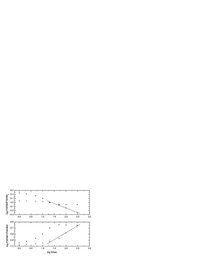
Figure 6: Prediction on the relationship between the width of pulses and energy (the upper panel) and that between the ratio of the $FWHM$ width of the rising portion to that of the decaying phase of the light curve of pulses and energy (the lower panel) for the typical hard (crosses) and soft (filled circles) bursts in the case that the indexes and the peak energy of the rest frame Band function spectrum decrease with time. The widths are calculated from the light curve of (2) arising from local Gaussian pulse (3), confined within channels A, B, C, D, E, F, G, and H, respectively, where we adopt $\Delta\tau_{\theta,FWHM}=0.1$, and we take $\Gamma=200$ and $\Gamma=20$ for the typical hard and soft bursts, respectively. The solid line is the power law curve deduced from the data of the BATSE channels for the typical hard burst.

We find from sample 1 that the medians of the distribution of the uncertainty of the three parameters are $\sigma_{E_{p}}=33.1keV$, $\sigma_{\alpha}=0.136$, and $\sigma_{\beta}=0.196$, respectively, while the medians of the distribution of the deviation (in absolute values) of the data from the regression lines deduced above for the three parameters are $|\Delta E_{p}|=97.0keV$, $|\Delta\alpha|=0.297$, and $|\Delta\beta|=0.410$, respectively. It shows that, in terms of statistics, the measurement uncertainties are generally less than the dispersions of data of the three parameters. In this section, we are interested only in the general manner of the developments of the three parameters. Therefore, considering the development manner illustrated above (represented by the regression lines) is enough. Thus, let us consider a typical evolution of rest frame indexes $\alpha_{0}$, $\beta_{0}$ and peak energy $E_{0,p}$ following $\alpha_{0}=-0.63-0.20(\tau_{\theta}-\tau_{\theta,1})/(\tau_{\theta,2}-\tau_{\theta,1})$, $\beta_{0}=-2.44-0.42(\tau_{\theta}-\tau_{\theta,1})/(\tau_{\theta,2}-\tau_{\theta,1})$ and $log(E_{0,p}/keV)=-0.06-0.16(\tau_{\theta}-\tau_{\theta,1})/(\tau_{\theta,2}-\tau_{\theta,1})$, for $\tau_{\theta,1}\leq\tau_{\theta}\leq\tau_{\theta,2}$ (to deduce the last formula, the previously adopted relation $E_{p}\simeq 1.67\Gamma E_{0,p}$ is applied to the typical hard burst for which the Lorentz factor is assumed to be $\Gamma=200$). For $\tau_{\theta}<\tau_{\theta,1}$, $\alpha_{0}=-0.63$, $\beta_{0}=-2.44$ and $log(E_{0,p}/keV)=-0.06$, while for $\tau_{\theta}>\tau_{\theta,2}$, $\alpha_{0}=-0.83$, $\beta_{0}=-2.86$ and $log(E_{0,p}/keV)=-0.22$. As mentioned above, we employ local Gaussian pulse (3) with $\Delta\tau_{\theta,FWHM}=0.1$ and assign $\tau_{\theta,0}=10\sigma+\tau_{\theta,\min}$ and $\tau_{\theta,\min}=0$ to study the relationship. We adopt $\tau_{\theta,1}=9\sigma+\tau_{\theta,\min}$ and $\tau_{\theta,2}=11\sigma+\tau_{\theta,\min}$. Corresponding relationships obtained in this situation are displayed in Fig. 6. The deviation shown above could also be observed in this figure. For the typical soft burst, the power law range shifts to the Swift band as well. We find that the power law index in the BATSE channels for the typical hard burst is within $-0.27$ — $-0.08$.

It is noticed that the peaked feature suggested above does not show. Instead, both the lower and higher band platforms shown in Figs. 4a and 4b remain. This might be due to the small speed of the development of the rest frame spectrum considered here (see what discussed below).

4 The relationship shown in individual pulses of a BATSE GRB sample

Presented in Kocevski et al. (2003) is a sample (the KRL sample) of FRED pulse GRBs. We consider only the first pulse of each burst since it is this pulse that is more closely associated with the initial condition of the event and might be less affected by environment. In addition, we limit our study on the sources for which the values of the peak energy are available and the corresponding signals are obvious enough so that the pulse widthes of at least three channels of BATSE could be well estimated. We find 28 bursts in the KRL sample that could meet these requirements. For these sources, the peak energy values are taken from Mallozzi et al. (1995). To find the central values of data of the light curve, we simply adopt equation (22) of Kocevski et al. (2003) to fit the corresponding light curve since we find that the form of the function could well describe the observed profile of a FRED pulse. The pulse width in each channel of BATSE is then estimated with the fitting parameters.

The estimated values of the $FWHM$ of the 28 GRB pulses in various energy channels are presented in Table 3. Relationships between the pulse width and energy for these pulses are shown in Fig. 7. Plotted in Fig. 7 are also the limits of the corresponding power law ranges of these pulses estimated with their peak energies according to the relations of $logE_{low}-logE_{p}\simeq(-1.10\sim-1.02)$ and $logE_{high}-logE_{p}\simeq(0.157\sim 0.177)$ which are deduced from the typical rest frame Band function spectrum with $\alpha_{0}=-1$ and $\beta_{0}=-2.25$ (see section 2.1), where only the largest value of $E_{low}$ and the smallest value of $E_{high}$ associated with the provided value of $E_{p}$ are presented.

From Fig. 7 we find:

a) a power law range could be observed in 13 sources: #907, #914, #1406, #1733, #1883, #2083, #2483, #2665, #2919, #3143, #3954, #4157, #5495;

b) a lower band platform could be observed or suspected in 8 bursts: #973, #1773, #1883, #1956, #2919, #3143, #4157, #5495;

c) a higher band platform could be observed or suspected in 6 sources: #907, #2083, #2387, #2484, #3886, #3892;

d) a peaked feature could be observed or suspected in 10 GRBs: #1467, #2102, #2880, #3155, #3870, #3875, #3954, #5478, #5517, #5523.

Among the 28 sources, those belonging to the platform-power-law-platform feature group include #907, #914, #973, #1406, #1733, #1883, #1956, #2083, #2387, #2484, #2665, #2919, #3143, #3886, #3892, #4157, and #5495. Those belonging to the peaked feature class are #1467, #2102, #2880, #3155, #3870, #3875, #3954, #5478, #5517, and #5523. This suggests that the features shown in the relationship obtained from the 27 sources (called normal bursts) are those predicted by the Doppler effect of fireballs. The only exception is #5541 which shows a sinkage, instead of a peaked, feature in the relationship, which is not a result in our analysis.

In addition, we find that, for 14 bursts (#907, #914, #1406, #1733, #1883, #2083, #2387, #2484, #2665, #2919, #3143, #3892, #3954, and #5495), the power law ranges expected from that associated with the typical rest frame Band function spectrum with $\alpha_{0}=-1$ and $\beta_{0}=-2.25$ and the provided value of $E_{p}$ are consistent with what derived from the observational data. For other normal bursts (there are 13), the two power law ranges are not in agreement. Among these 13 normal bursts, the power law range of #3886 is in a lower energy band than its $E_{p}$ suggests, while for others, the power law range is in a higher energy band than the provided value of $E_{p}$ confines. If the relation (that is associated with the typical rest frame Band function spectrum with $\alpha_{0}=-1$ and $\beta_{0}=-2.25$) used to derive the power law range with the provided value of $E_{p}$ is approximately applicable to these sources, the difference could be explained by assuming that the peak energies of these bursts have been less estimated. This assumption might be true since peak energies are always measured from time-integral spectra which must shift to a lower energy band from the hardest spectra of the sources. Under this interpretation, only the problem of the behavior of #3886 is unsolved.

5 Discussion and conclusions

In this paper, we study in details how the pulse width $FWHM$ and the ratio of the rising width to the decaying width $FWHM1/FWHM2$ of GRBs are related with energy under the assumption that the sources are in the stage of fireballs which expand relativistically.

It can be concluded from our analysis that: a) owing to the Doppler effect of fireballs, it is common that there exists a power law relationship between $FWHM$ and energy and between $FWHM1/FWHM2$ and energy within a limited range of frequency; b) the power law range and index depend strongly on the rest frame radiation form as well as the observed peak energy (the range could span over more than one to five orders of magnitudes of energy for different rest frame spectra); c) the upper and lower limits of the power law range can be determined by the observed peak energy $E_{p}$; d) in cases when the development of the rest frame spectrum could be ignored, a platform-power-law-platform feature would be formed, while in cases when the rest frame spectrum is obviously softening with time, a peaked feature would be observed. In addition, we find that local pulse forms affect only the magnitude of the width and the ratio of widthes.

We perform predictions on the relationships for a typical hard burst with $\Gamma=200$ and a typical soft burst with $\Gamma=20$. The analysis shows that, generally, for the typical hard burst the power range would be observed in the BATSE band while for the typical soft burst the power law range would shift to the Swift band. In some particular cases (e.g., when the rest frame thermal synchrotron spectrum is adopted), the power law range could cover the BATSE as well as Swift bands for both typical bursts.

A sample of 28 GRBs is employed to study the relationship. We find that, except #5541, sources of the sample either exhibit the platform-power-law-platform feature (including 17 bursts) or show the peaked feature (including 10 bursts). It suggests that, for most sources of this sample, the Doppler effect of fireballs could indeed account for the observed relationship. As for #5541, we wonder if other kinds of rest frame spectral evolution such as a soft-to-hard-to-soft manner instead of the simple decreasing pattern could lead to its specific feature (it will deserve an investigation later). Since the peaked feature is a signature of the development of the rest frame spectrum, we suspect that the 10 sources with the peaked feature might undergo an obvious evolution of radiation, while for the other 17 bursts, the development, if it exists, might be very mild.

In the above analysis, we consider the evolution of three parameters, the lower and higher energy indexes and the peak energy, of the rest frame Band function spectrum. We wonder what a role each of the three factors would play in producing the peaked feature shown above. Here we study once more the case of the simple evolution of indexes $\alpha_{0}$ and $\beta_{0}$ and peak frequency $\nu_{0,p}$ considered in section 2.3, but in three different patterns. They are as follows: a) $\alpha_{0}=-0.5-(\tau_{\theta}-\tau_{\theta,1})/(\tau_{\theta,2}-\tau_{\theta,1})$ for $\tau_{\theta,1}\leq\tau_{\theta}\leq\tau_{\theta,2}$, and $\alpha_{0}=-0.5$ for $\tau_{\theta}<\tau_{\theta,1}$, and $\alpha_{0}=-1.5$ for $\tau_{\theta}>\tau_{\theta,2}$, and $\beta_{0}=-2$ and $log\nu_{0,p}=0.1$; b) $\beta_{0}=-2-(\tau_{\theta}-\tau_{\theta,1})/(\tau_{\theta,2}-\tau_{\theta,1})$ for $\tau_{\theta,1}\leq\tau_{\theta}\leq\tau_{\theta,2}$, and $\beta_{0}=-2$ for $\tau_{\theta}<\tau_{\theta,1}$, and $\beta_{0}=-3$ for $\tau_{\theta}>\tau_{\theta,2}$, and $\alpha_{0}=-0.5$ and $log\nu_{0,p}=0.1$; c) $log\nu_{0,p}=0.1-(\tau_{\theta}-\tau_{\theta,1})/(\tau_{\theta,2}-\tau_{\theta,1})$ for $\tau_{\theta,1}\leq\tau_{\theta}\leq\tau_{\theta,2}$, and $log\nu_{0,p}=0.1$ for $\tau_{\theta}<\tau_{\theta,1}$, and $log\nu_{0,p}=1.1$ for $\tau_{\theta}>\tau_{\theta,2}$, and $\alpha_{0}=-0.5$ and $\beta_{0}=-2$. The first pattern is associated with the evolution of the lower energy index, the second reflects nothing but the evolution of the higher energy index, and the third connects with the evolution of the peak energy, of the rest frame Band function spectrum, where, for each of the three cases, the other two parameters are fixed. In the same way we employ local Gaussian pulse (3) with $\Delta\tau_{\theta,FWHM}=0.1$ to study the relationship. We adopt $\Gamma=100$, $\tau_{\theta,1}=9\sigma+\tau_{\theta,\min}$ and $\tau_{\theta,2}=11\sigma+\tau_{\theta,\min}$, and assign $\tau_{\theta,0}=10\sigma+\tau_{\theta,\min}$ and $\tau_{\theta,\min}=0$. Displayed in Fig. 8 are the corresponding $FWHM$ — $\nu/\nu_{0,p,max}$ and $FWHM1/FWHM2$ — $\nu/\nu_{0,p,max}$ curves, where $\nu_{0,p,max}$ is the largest value of $\nu_{0,p}$ adopted. One finds from Fig. 8 that the peaked feature shown in the relationship between the width and energy (see Fig. 3) is mainly due to the evolution of the lower energy index of the rest frame Band function spectrum, while that shown in the relationship between the ratio of pulse widths and energy arises from the evolution of the higher energy index. It is interesting that no contribution from the evolution of the peak energy of the rest frame Band function spectrum to the features could be detected (probably the evolution of the peak energy considered here is too mild to produce an interesting feature).

As mentioned above, it was proposed by many authors that the power law relationship observed in GRB pulses could arise from synchrotron radiation (see section 1). A simple synchrotron cooling scenario is: as the electrons cool, their average energy becomes smaller, which causes the emission peaks at lower energy at later time (see Kazanas et al. 1998). Recently, a power law relationship between the total isotropic energy and $E_{p}$ was revealed (Lloyd et al. 2000; Amati et al. 2002). It was suggested that this power law relation could be expected in the case of an optically thin synchrotron shock model for a power law distribution of electrons (see Lloyd et al. 2000). These considerations lead to a softening picture of the rest frame spectrum.

Does the proposal of synchrotron radiation conflict with the effect discussed above? To find an answer to this, it might be helpful to remind that the Doppler effect of fireballs is only a kinetic effect while that of synchrotron radiation is a dynamic one. Therefore, there is no confliction between the two. As analyzed in section 2.3, a softening of the rest frame spectrum coupling with the Doppler effect of fireballs would lead to a peaked feature in the relationship between the pulse width and energy if the speed of the softening is fast enough. The observed data of our sample (see Fig. 7) show that this is indeed the case for some events (at least for some FRED pulse GRBs).

We are wondering if the softening of the rest frame spectrum could lead to a much different value of the power law index. We thus analyze the power law ranges in the upper panels of Fig. 3 and find that the index would be confined within $-0.27$ — $-0.18$, which is not much different from what obtained above.

We know that light curves of most bursts are complex and do not consists of single pulses. It was pointed out that superposition of many pulses could create the observed diversity and complexity of GRB light curves (Fishman et al. 1994; Norris et al. 1996; Lee et al. 2000a, 2000b). Could our analysis be applied to all light curves observed in GRBs? The answer is no. The Doppler effect of firteballs is associated with the angular spreading timescale which is proportional to $1/2\Gamma^{2}$ (see, e.g., Kobayashi, Piran, & Sari 1997; Piran 1999; Nakar & Piran 2002; Ryde & Petrosian 2002). Our model would not be applicable to light curves of multi-pulses which are separated by timescales larger the angular spreading timescale.

What would happen if local pulses are close enough? Let us consider a local pulse comprising three Gaussian forms:

$$\widetilde{I}(\tau_{\theta})=\\ I_{0,1}\exp[-(\frac{\tau_{\theta}-\tau_{\theta,0,1}}{\sigma_{1}})^{2}]+I_{0,2}\exp[-(\frac{\tau_{\theta}-\tau_{\theta,0,2}}{\sigma_{2}})^{2}]+I_{0,3}\exp[-(\frac{\tau_{\theta}-\tau_{\theta,0,3}}{\sigma_{3}})^{2}]\qquad(\tau_{\theta,\min}\leq\tau_{\theta}),$$ (7)

where $I_{0,1}$, $I_{0,2}$, $I_{0,3}$, $\sigma_{1}$, $\sigma_{2}$, $\sigma_{3}$, $\tau_{\theta,0,1}$, $\tau_{\theta,0,2}$, $\tau_{\theta,0,3}$, and $\tau_{\theta,\min}$ are constants. We calculate light curves of (2) arising from local pulse (7) and emitted with the typical rest frame Band function spectral form with $\alpha_{0}=-1$ and $\beta_{0}=-2.25$, adopting $I_{0,1}=0.15$, $I_{0,2}=0.2$, $I_{0,3}=0.04$, $\sigma_{1}=0.3$, $\sigma_{2}=0.2$, $\sigma_{3}=0.2$, $\tau_{\theta,0,1}=5\sigma_{1}+\tau_{\theta,\min}$, $\tau_{\theta,0,2}=\tau_{\theta,0,1}+4\sigma_{1}$, $\tau_{\theta,0,3}=\tau_{\theta,0,2}+7\sigma_{2}$, $\nu_{0,p}=0.75keVh^{-1}$, and $\Gamma=200$, and assigning $\tau_{\theta,\min}=0$. Shown in Fig. 9 are the corresponding light curves in channels A, B, C, D, E, F, G, and H, respectively, and presented in Fig. 10 are the relationships between $FWHM/FWHM_{E}$ and $E/keV$ and between $FWHM1/FWHM2$ and $E/keV$ deduced from these light curves. We find no significant difference between these relationships and those in Fig. 4 (the data of the typical hard burst there).

It should be pointed out that in this paper we are interested in cases where the Doppler effect of fireballs is important and thus we examine only FRED pulse sources. It would not be surprised if the results are not applicable to other forms of pulses. In the case when the mentioned effect is not at work, a power law relationship might also exist. If so, synchrotron radiation might be responsible to the observed relationship. This, we believe, also deserves a detailed investigation (probably, in this case, the pulses concerned should be non-FRED ones).

Figure 1: Relationships between the $FWHM$ width and energy (a) and between the ratio $FWHM1/FWHM2$ and energy (b) for the light curve of (2) confined within $0.99\nu/\nu_{0,p}\leq\nu/\nu_{0,p}\leq 1.01\nu/\nu_{0,p}$, in the case of adopting the Band function with $\alpha_{0}=-1$ and $\beta_{0}=-2.25$ as the rest frame radiation form and the Gaussian pulse as its local pulse. Where dot lines from the bottom to the top represent the curves associated with $\Delta\tau_{\theta,FWHM}=0.01$, $0.1$, $1$, $10$, respectively, for $\Gamma=10$; solid lines from the bottom to the top represent the curves associated with $\Delta\tau_{\theta,FWHM}=0.01$, $0.1$, $1$, $10$, respectively, for $\Gamma=100$; dash lines from the bottom to the top stand for the curves associated with $\Delta\tau_{\theta,FWHM}=0.01$, $0.1$, $1$ , $10$, respectively, for $\Gamma=1000$. Shown in panels (c) and (d) are the curves in panels (a) and (b) respectively, where the corresponding energy is presented in units of $keV$. The two vertical dash dot lines in (c) and (d) denote the power law ranges deduced from the curves associated with the case of $(\Gamma,\Delta\tau_{\theta,FWHM})=(100,10)$.

Figure 2: Relationships between the $FWHM$, $FWHM1/FWHM2$ of pulses and energy for the light curve of (2) confined within $0.99\nu/\nu_{0,p}\leq\nu/\nu_{0,p}\leq 1.01\nu/\nu_{0,p}$, in the case of adopting the thermal synchrotron spectrum (left panels) and Comptonized spectrum (right panels) as the rest frame radiation form and the Gaussian pulse as its local pulse. Where dot lines from the bottom to the top represent the curves associated with $\Delta\tau_{\theta,FWHM}=0.01$, $0.1$, $1$, $10$, respectively, for $\Gamma=10$; solid lines from the bottom to the top represent the curves associated with $\Delta\tau_{\theta,FWHM}=0.01$, $0.1$, $1$, $10$, respectively, for $\Gamma=100$; dash lines from the bottom to the top stand for the curves associated with $\Delta\tau_{\theta,FWHM}=0.01$, $0.1$, $1$ , $10$, respectively, for $\Gamma=1000$.

Figure 3: Relationship between the $FWHM$ width of pulses and energy (upper panels) and that between $FWHM1/FWHM2$ and energy (lower panels) for the light curve of (2) confined within $0.99\nu/\nu_{0,p}\leq\nu/\nu_{0,p}\leq 1.01\nu/\nu_{0,p}$, in the case of adopting the varying Band function (see section 2.3) as the rest frame radiation form and Gaussian pulse (3) with $\Delta\tau_{\theta,FWHM}=0.1$ as its local pulse, for $\Gamma=10$ (left panels), $100$ (mid panels), $1000$ (right panels), respectively, where $\nu_{0,p,max}=10^{0.1}$. The dotted, dashed and solid lines represent the curves with $k=0.1$, $0.5$ and $1.0$, respectively.

Figure 4: Prediction on the relationship between the width of pulses and energy (upper panels) and that between the ratio of the $FWHM$ width of the rising portion to that of the decaying phase of the light curve of pulses and energy (lower panels) for the typical hard (crosses) and soft (filled circles) bursts. The widths are deduced from the light curve of (2) associated with the local Gaussian pulse and the rest frame Band function with $\alpha_{0}=-1$, $\beta_{0}=-2.25$ and $\nu_{0,p}=0.75keVh^{-1}$ (left panels), thermal synchrotron spectrum with $\nu_{0,s}=3.5\times 10^{-3}keVh^{-1}$ (mid panels), and Comptonized spectrum with $\alpha_{0,C}=-0.6$, $\nu_{0,C}=0.55keVh^{-1}$ (right panels), confined within channels A, B, C, D, E, F, G, and H, respectively, where we adopt $\Delta\tau_{\theta,FWHM}=0.1$ and take $\Gamma=200$ and $\Gamma=20$ for typical hard and soft bursts, respectively. The solid line is the power law curve deduced from the data of the BATSE channels for the typical hard burst. Open squares in left panels represent the expected data of Beppo-SAX and open circles filled with pluses stand for those of Hete-II.

Figure 5: Developments of the low, high energy indexes and the peak energy of sample 1 in terms of a relative time scale, where $t_{min}$ and $t_{max}$ are the lower and the upper limits of the observation time of individual sources. The solid line is the regression line.

Figure 7: Relationship between the observed $FWHM$ width of pulses and energy shown in the BATSE energy range for the 28 GRBs concerned, where for some bursts the widths in all the 4 BATSE channels are known while for others only the widths in 3 channels are available. The dashed vertical line represents the expected lower limit $E_{low}$ of the power law range and the solid vertical line stands for the higher limit $E_{high}$, which are associated with the typical rest frame Band function spectrum with $\alpha_{0}=-1$ and $\beta_{0}=-2.25$ and the provided value of $E_{p}$.

Figure 8: Relationship between the $FWHM$ of pulses and energy (upper panels) and that between the ratio $FWHM1/FWHM2$ and energy (lower panels) for the light curve of (2) confined within $0.99\nu/\nu_{0,p}\leq\nu/\nu_{0,p}\leq 1.01\nu/\nu_{0,p}$, in the case of adopting various patterns of development of the Band function as the rest frame radiation form and Gaussian pulse (3) with $\Delta\tau_{\theta,FWHM}=0.1$ as its local pulse and taking $\Gamma=100$ and $k=1.0$. Solid lines in the two left panels represent the curves associated with the case when only the lower energy index varies with time; solid lines in the two mid panels represent those associated with the case when only the higher energy index varies with time; solid lines in the two right panels stand for those associated with the case when only the peak energy varies with time. The dotted lines represent the corresponding curves with $\Gamma=100$ and $k=1.0$ in Fig. 3 (see solid lines in the mid panels of Fig. 3).

Figure 9: Light curves in channels B, E, A, C, D, F, G, and H (solid lines from the top to the bottom) for the typical hard burst ($\Gamma=200$). The curves are calculated with equation (2) when adopting the local pulse comprising three Gaussian forms shown by equation (7) and the rest frame Band function with $\alpha_{0}=-1$, $\beta_{0}=-2.25$ and $\nu_{0,p}=0.75keVh^{-1}$.

Figure 10: Prediction on the relationship between the width of pulses and energy (the upper panel) and that between the ratio of the $FWHM$ width of the rising portion to that of the decaying phase of the light curve of pulses and energy (the lower panel) for the typical hard burst. The widths are deduced from the light curves of Fig. 9.

Table 1: Turning frequency and typical width obtained from the curves in Fig. 1a

$\Gamma$	$\Delta\tau_{\theta,FWHM}$	log$\frac{\upsilon_{low}}{\upsilon_{0,p}}$	log$\frac{\upsilon_{high}}{\upsilon_{0,p}}$	$logFWHM_{min}$	$logFWHM_{min}$
	0.01	0.20	1.39	-2.87	-2.64
10	0.1	0.17	1.38	-2.59	-2.39
	1	0.13	1.38	-1.84	-1.66
	10	0.12	1.38	-0.88	-0.71
	0.01	1.20	2.40	-4.87	-4.64
100	0.1	1.17	2.40	-4.59	-4.39
	1	1.14	2.38	-3.84	-3.66
	10	1.13	2.38	-2.88	-2.71
	0.01	2.20	3.40	-6.87	-6.64
1000	0.1	2.18	3.39	-6.59	-6.39
	1	2.14	3.38	-5.84	-5.66
	10	2.13	3.39	-4.88	-4.71

Table 2: Turning frequency and typical width obtained from the curves in Fig. 1b

$\Gamma$	$\Delta\tau_{\theta,FWHM}$	log$\frac{\upsilon_{low}}{\upsilon_{0,p}}$	log$\frac{\upsilon_{high}}{\upsilon_{0,p}}$	$log(\frac{FWHM1}{FWHM2})_{min}$	$log(\frac{FWHM1}{FWHM2})_{max}$
	0.01	0.20	1.38	-1.57	-1.36
10	0.1	0.16	1.37	-0.89	-0.69
	1	0.13	1.37	-0.63	-0.44
	10	0.12	1.37	-0.59	-0.41
	0.01	1.19	2.39	-1.57	-1.35
100	0.1	1.16	2.36	-0.89	-0.69
	1	1.13	2.36	-0.63	-0.44
	10	1.12	2.36	-0.59	-0.41
	0.01	2.19	3.39	-1.57	-1.35
1000	0.1	2.16	3.36	-0.89	-0.69
	1	2.13	3.35	-0.63	-0.44
	10	2.12	3.37	-0.59	-0.41

Table 3: Estimated values of the $FWHM$ of the four BATSE channels for the 28 GRB sources

trigger	$W1$	$\sigma_{W1}$	$W2$	$\sigma_{W2}$	$W3$	$\sigma_{W3}$	$W4$	$\sigma_{W4}$
907			6.791	0.898	3.826	0.338	2.441	0.212
914	3.915	0.176	2.562	0.159	1.269	0.350
973	7.874	4.530E-6	7.177	0.393	7.072	1.818E-2	5.008	0.360
1406	11.375	9.846E-6	9.765	6.605-2	8.041	5.820
1467	6.400	0.735	7.053	1.178E-6	5.984	0.569
1733	4.989	0.910	4.463	0.454	4.069	0.746	3.308	0.896
1883	3.874	0.106	3.288	0.0207	2.585	0.067	1.325	0.053
1956	4.920	2.762E-2	4.812	0.326	3.897	0.573
2083	3.961	1.675E-4	2.365	1.124	0.892	0.424	0.720	0.206
2102	3.488	0.424	4.119	1.001	3.526	0.477
2387	18.447	1.295	15.602	1.229	15.085	0.667
2484	7.081	2.503	5.241	1.054	4.687	3.200E-2
2665	7.205	0.312	5.814	0.367	4.391	0.409
2880	1.319	3.360E-2	1.365	9.737E-2	1.150	2.748E-2
2919	4.257	8.533E-2	3.714	0.502	2.906	0.942	1.045	0.429
3143	2.238	0.329	1.908	2.617	1.334	0.101
3155	0.925	0.592	1.229	1.280	1.044	0.302
3870	1.842	2.419E-2	2.312	1.514E-2	1.336	1.264E-2
3875	0.759	1.751E-2	1.088	0.111	0.592	0.367
3886	0.954	3.857E-2	0.661	5.198E-2	0.666	8.197E-2
3892	2.979	2.973E-2	1.609	0.180	1.383	0.185
3954	2.962	1.125	2.533	0.577	2.602	0.379	0.941	0.0860
4157	5.368	1.149	4.209	0.470	1.014	5.743E-2
5478	5.052	0.680	6.267	0.251	4.246	0.190
5495	1.929	3.197E-4	1.740	2.940E-2	1.096	9.084E-2
5517	3.004	1.032	3.146	1.296	2.156	5.173E-2
5523	3.877	5.971E-2	4.257	0.488	3.028	2.176E-2
5541	4.420	6.866E-2	3.744	1.090	4.862	5.372E-2

Note — $W1$, $W2$, $W3$, and $W4$ are the $FWHM$ of pulses in the first ($20-50kev$), second ($50-100kev$), third ($100-300kev$), and fourth ($>300kev$) energy channels of BATSE, respectively.

References

• Amati et al. (2002) Amati, L., Frontera, F., Tavani, M. et al. 2002, A&A, 390, 81
• Band et al. (1993) Band, D., Matteson, J., Ford, L. et al. 1993, ApJ, 413, 281
• Chiang (1998) Chiang, J., 1998, ApJ, 508, 752
• Cohen et al. (1997) Cohen, E., Katz, J. I., Piran, T., & Sari, R. 1997, ApJ, 488, 330
• Costa (1998) Costa, E. 1998, Nuclear Physics B (Proc. Suppl.), 69/1-3, 646
• Crew et al. (2003) Crew, G. B., Lamb, D. Q., Ricker, G. R., Atteia, J.-L., Kawai, N., et al. 2003, ApJ, 599, 387
• Dado et al. (2002a) Dado, S., Dar, A., and De Rujula, A. 2002a, A&A, 388, 1079
• Dado et al. (2002b) Dado, S., Dar, A., and De Rujula, A. 2002b, ApJ, 572, L143
• Dermer (1998) Dermer, C. D. 1998, ApJ, 501, L157
• Eriksen & Gron (2000) Eriksen, E., & Gron, O. 2000, Amer. J. Phys., 68, 1123
• Fenimore et al. (1995) Fenimore, E. E., in’t Zand, J. J. M., Norris, J. P. et al. 1995, ApJ, 448, L101
• Fenimore et al. (1996) Fenimore, E. E., Madras, C. D., Nayakshin, S. 1996, ApJ, 473, 998
• Feroci et al. (2001) Feroci, M., Antonelli, L. A., Soffitta, P., In’t Zand, J. J. M., Amati, L., et al. 2001, A&A, 378, 441
• Fishman et al. (1992) Fishman, G., et al. 1992, in Gamma-Ray Bursts: Huntsville, 1991, ed. W. S. Paciesas & G. J. Fishman (New York: AIP), 13
• Fishman et al. (1994) Fishman, G. J., Meegan, C. A., Wilson, R. B. et al. 1994, ApJS, 92, 229
• Goodman (1986) Goodman, J. 1986, ApJ, 308, L47
• Granot et al. (1999) Granot, J., Piran, T., Sari, R. 1999, ApJ, 513, 679
• Hailey et al. (1999) Hailey, C. J., Harrison, F. A., Mori, K. 1999, ApJ, 520, L25
• Kazanas et al. (1998) Kazanas, D., Titarchuk, L. G., & Hua, X.-M. 1998, ApJ, 493, 708
• Kobayashi et al. (1997) Kobayashi, S., Piran, T., & Sari, R. 1997, ApJ, 490, 92
• Kocevski et al. (2003) Kocevski, D., Ryde, F., Liang, E. 2003, ApJ, 473, 998
• Krolik & Pier (1991) Krolik, J. H., & Pier, E. A. 1991, ApJ, 373, 277
• Lee et al. (2000a) Lee, A., Bloom, E. D., & Petrosian, V. 2000a, ApJS, 131, 1
• Lee et al. (2000b) Lee, A., Bloom, E. D., & Petrosian, V. 2000b, ApJS, 131, 21
• Liang et al. (1983) Liang, E. P., Jernigan, T. E., Rodrigues, R. 1983, ApJ, 271, 766
• Link, Epstein, & Priedhorsky (1993) Link, B., Epstein, R. I., & Priedhorsky, W. C. 1993, ApJ, 408, L81
• Lloyd et al. (2000) Lloyd, N. M., Petrosian, V., Mallozzi, R. S. 2000, ApJ, 534, 227
• Mallozzi et al. (1995) Mallozzi, R.S., Paciesas, W.S., Pendleton, G.N., et al. 1995, Apj, 454, 597
• Meszaros & Rees (1998) Meszaros, P., & Rees, M. J. 1998, ApJ, 502, L105
• Nakar & Piran (2002) Nakar, E., & Piran, T. 2002, ApJ, 572, L139
• Nemiroff (2000) Nemiroff, R. J. 2000, ApJ, 544, 805
• Norris et al. (1996) Norris, J. P., Nemiroff, R. J., Bonnell, J. T. et al. 1996, ApJ, 459, 393
• Norris et al. (2000) Norris, J. P., Marani, G. F., Bonnell, J. T. 2000, ApJ, 534, 248
• Paczynski (1986) Paczynski, B. 1986, ApJ, 308, L43
• Piran (1999) Piran, T. 1999, Phys. Rep., 314, 575
• Piro et al. (1998) Piro, L., Heise, J., Jager, R., Costa, E., Frontera, F., et al. 1998, A&A, 329, 906
• Preece et al. (2000) Preece, R. D., Briggs, M. S., Mallozzi, R. S. et al. 2000, ApJS, 126, 19
• Qin (2002) Qin, Y.-P. 2002, A&A, 396, 705
• Qin (2003) Qin, Y.-P. 2003, A&A, 407, 393
• Qin et al. (2004) Qin, Y.-P., Zhang, Z.-B., Zhang, F.-W., Cui, X.-H. 2004, ApJ, 617, 439 (Paper I)
• Ryde & Petrosian (2002) Ryde, F., & Petrosian, V. 2002, ApJ, 578, 290
• Schaefer et al. (1994) Schaefer, B. E., Teegarden, B. J., Fantasia, S. F., et al. 1994, ApJS, 92, 285
• Shen et al. (2005) Shen, R.-F., Song, L.-M., Li, Z. 2005, MNRAS, in press (astro-ph/0505276)
• Strohmayer et al. (1998) Strohmayer, T. E., Fenimore, E. E., Murakami, T., Yoshida, A. 1998, ApJ, 500, 873
• Wang et al. (2000) Wang, J. C., Cen, X. F., Qian, T. L., Xu, J., & Wang, C. Y. 2000, ApJ, 532, 267
Refer to caption