Observation of EGRET Gamma-Ray Sources by an Extensive Air Shower Experiment

Ultra-high-energy (E$>$100 Tev) Extensive Air Showers (EASs) have been monitored for a period of five years (1997 - 2003), using a small array of scintillator detectors in Tehran, Iran. The data have been analyzed to take in to account of the dependence of source counts with respect to the zenith angle. During a calendar year different sources come in the field of view of the detector at varying zenith angles. Because of varying thickness of the overlaying atmosphere, the shower count rate is extremely dependent on zenith angle which have been carefully analyzed over time. (Bahmanabadi et al. (2002)).High energy gamma-ray sources from EGRET third catalogue where observed and the data were analyzed using an excess method. A number of upper limits for a number of EGRET sources were obtained, including 6 AGNs or probably AGNs and 4 unidentified sources.

1 Introduction

EGRET instrument on-board $Compton\hskip 2.84526ptGamma\hskip 2.84526ptRay\hskip 2.84526ptObservatory\hskip 2.84526pt(CGRO)$ has detected both diffuse and discrete gamma-ray emission. The diffuse emission is both galactic (Hunter et al. (1997)) and extra-galactic in nature (Sreekumar et al. (1998)). EGRET has detected about 271 high energy ($>$100 MeV) gamma-ray sources (Hartman et al. (1999)). Besides AGNs these sources include 170 sources that are not identified conclusively with unique counterparts in other wavelengths. Two third of these EGRET unidentified (EUI) sources lie close to the galactic plane-potential counterparts (Bhattacharya et al. (2003)) for these include young pulsars, young radio quiet pulsars (Torres et al. (2001), D’Amico et al. (2001), Zhang et al. (2000)), Wolf Rayet (WR) stars, Of stars, OB associations (Romero et al. (1999)), Super Nova Remnants (SNRs) (Combi et al. (2001), Case & Bhattacharya (1998), Sturner & Dermer (1995)) and other types of sources.
Some other faint sources are in the mid-latitude region suggested to be associated with the Gould Belt (Gehrels et al. (2000)), which underwent an intense star formation period about sixty million years ago (Grainer (2000), Harding & Zhang (2001)). High latitude sources which are about 50, might be galactic gamma-ray halo sources (Dixon et al. (1998)) or unidentified sources are thought to be extra-galactic. These extra-galactic EUI sources contain Blazars and Active Galactic Nuclei (AGNs), galaxy clusters (Colafrancesco, S., (2002)), BL Lacerta objects (Torres et al. (2003)) and other types.
Whether the EGRET sources have emission in higher energies, is an interesting question (Lamb & Macomb (1997)). Gamma-ray with energies about 100 TeV and more entering the earth atmosphere, produce Extensive Air Showers (EASs) (Gaisser, T.K., (1990)) which could be observed by the detection of the secondary particles of the showers on the ground level (Bahmanabadi et al. (1998)). Previous attempts have been reported by other EAS arrays (Amenomori et al. (2002), tibet2000 (2000), Borione et al. (1997), Alexandreas et al. (1993), McKay et al. (1993) ).
This paper reports the results of a small particle detector array located at the Sharif University of Technology in Tehran. This small array is a prototype for a larger EAS array to be built at an altitude of 2600 m ($\equiv$ 756 g/cm²) at ALBORZ Observatory (AstrophysicaL oBservatory for cOsmic Radiation on alborZ) (see http://sina.sharif.edu/^∼observatory/ ) near Tehran. The prototype installed on the roof of physics department of Sharif University of Technology in Tehran, 1200 m ($\equiv$ 890 g/cm²), $35.72^{\circ}N$ and $51.33^{\circ}E$. In this work we present the observational results of 10 EGRET third catalogue sources, we describe the experimental setup in Section 2. the data analysis in Section 3, the results in Section 4. Section 5 is devoted to a discussion of the results.

2 Experimental arrangements

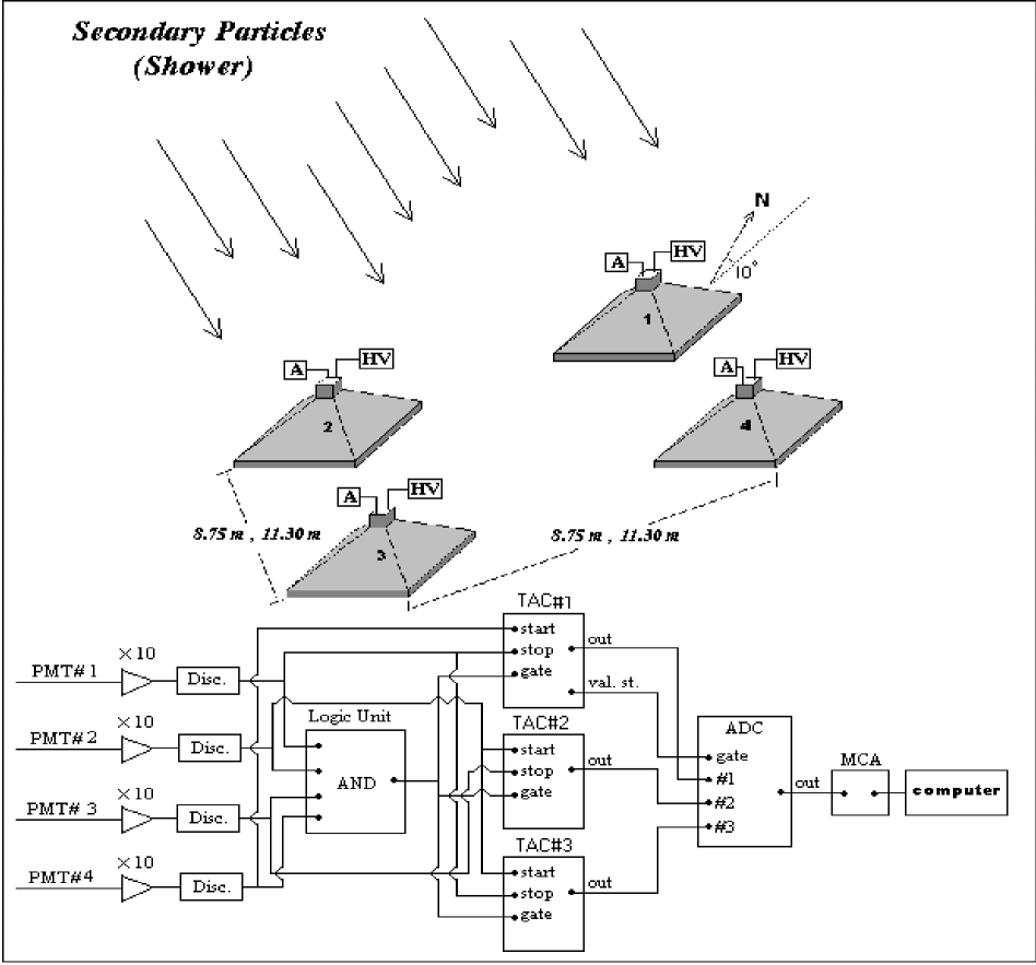
Figure 1: Experimental set up and electronic circuits.

The array is constructed of 4 slab plastic scintillators ($100\times 100\times 2$ cm³) as a square in Tehran (35^∘ 43${}^{{}^{\prime}}$ , 51^∘ 20${}^{{}^{\prime}}$), Iran, with The elevation 1200 m over sea level (890 g/cm²) which is shown in Fig. 1. All of the scintillators are on a flat level surface. Each scintillator is housed in a pyramidal steel box with height of 15 cm. The interior surface of each box is coated with white paint, (Bahmanabadi et al. (1998)) and a 5 cm diameter PMT(EMI 9813KB) is placed at the vertex of the pyramidal box. Fig. 1 shows a schematic diagram of the array and its electronic circuit to log each EAS event. After passing of at least one particle from a detector the PMT creates a signal with a pulse height which is related to the direction, number of the passed particles, and location of the crossed particles in the scintillator. The output signals from the PMTs are amplified in a one stage amplification ($\times$10) with an 8-fold fast amplifier (CAEN N412), and then transfer to an 8-fold fast discriminator (CAEN N413A) which is operated in a fixed level of 20mV one by one. The threshold of each discriminator is set at the separation point between the signal and background noise levels. Each discriminator has two outputs, one of them is connected to a coincidence logic unit (CAEN N455) as trigger condition. Trigger condition is satisfied when at least one charged particle passes through each of the four detectors within a time window of 150ns. The other discriminator output is connected to a Time to Amplitude Converter (TAC)(EG&G ORTEC 566) which are set to a full scale of 200ns (maximum time difference between each two scintillators which is acceptable). The outputs of the No.4 scintillator was connected to start input of TAC1 whereas the output of No.2 was connected to start inputs of TAC2 and TAC3. The Output of the scintillator No.3 was connected to the stop input of TAC2 and No.1 was connected to stop inputs of both TAC1 and TAC3. Then the outputs of these three TACs were fed into a multi parameter Multi Channel Analyzer (MCA)(KIAN AFROUZ Inc.) via an Analogue to Digital Converter (ADC)(KIAN AFROUZ Inc.) unit.
When all of the scintillators have coincidence pulses, these TACs are trigged by logic unit and 3 time lags between the output signals of PMTs (4,1), (2,3) and (2,1) are read out by a computer as parameters 1 to 3. So with this procedure an EAS event is logged.
Two different experimental configurations were used by the experimental set up. All of the experimental set up were identical in the first ($E1$) and the second ($E2$) experimental configurations except for the size of the array. In $E1$ the size was 8.75 m $\times$ 8.75 m and in $E2$ the size was $11.30$ m $\times$ $11.30$ m.

3 Data Analysis

The logged time lags between the scintillators and Greenwich Mean Time (GMT) of each EAS event were recorded as raw data. We synchronized our computer to GMT (see http://www.timeanddate.com ). Our electronic has record capability of 18.2 times per second or equivalently each 0.055 seconds one record will be stored regardless of the existence or non existence of EAS events. If an EAS event occurs, its three time lags will be recorded and if it does not occur ’zero’ will be recorded. Therefore with the starting time of each experiment and counting of these zero and non zero records we will obtain GMT time of each EAS event. Our detected EAS events are a mixture of cosmic-ray events and gamma-ray events. In $E1$ total number of EAS events was 53,907 and duration of the experiment was 501,460 seconds. So the mean event rate of the first experiment was 0.1075 events per second. The distribution of the time between successive events has a good agreement with an exponential function, indicating that the event sampling is completely random (Bahmanabadi et al. (2003)). In $E2$ total number of events was 173,765 and duration of the second experiment was 2,902,857 seconds. So its mean event rate was $0.05986$ events per second.
We refined the data for separation of acceptable events. Events are acceptable if there be a good coincidence between the four scintillator pulses. We omitted the events with zenith angles more than 60^∘. Therefore after the separation we obtained smaller data sets of 46,334 and 120,331 for $E1$ and $E2$ respectively. Since we can not determine the energy of the showers on an event by event basis, we estimate our lower energy threshold by comparing our event rate to a cosmic-ray integral spectrum (Borione et al. (1997))

$$J(E)=2.78\times 10^{-5}E^{-2.22}+9.66\times 10^{-6}E^{-1.62}-1.94\times 10^{-12}\hskip 8.53581pt40\leq E\leq 5000\hskip 2.84526pt{\rm TeV}$$ (1)

The obtained lower energy limits were 39 Tev in $E1$ and 54 TeV in $E2$. The calculated mean energies were 94 and 132 TeV in $E1$ and $E2$ respectively. If the well-known Hillas spectrum (Gaisser, T.K., (1990))

$$F(>E)\sim 2\times 10^{-10}\frac{particle}{cm^{2}\hskip 2.84526pts\hskip 2.84526ptsr}\times(\frac{E}{1000TeV})^{-\gamma}$$ (2)

is used the lower limits will be 40 TeV and 60 Tev. Since the distribution of cosmic-ray events within the array in these energy ranges are homogeneous and isotropic, we used an excess method (Amenomori et al. (2002), tibet2000 (2000)) to find signature of EGRET third catalogue gamma-ray sources. This method was used for both $E1$ and $E2$.
The complete analysis procedure is itemized as follows :

• The calculation of local coordinates; zenith and azimuth angles of each EAS event $(z,\varphi)$ were calculated using a least square method by logged time lags and coordinates of the scintillators.

• The local angle distributions of the EAS events were investigated to understand the general behaviours of these EAS events.

• The calculation of equatorial coordinates (RA,Dec) of each EAS event using its local coordinates, the GMT of the event and geographical latitude of the array. Then we calculated galactic coordinates (l,b) of each EAS event from its equatorial coordinates using epoch J2000.

• The estimation of angular errors in galactic coordinates of investigated EGRET sources by error factors of the array.

• The simulation of a homogeneous distribution of EAS events to investigate cosmic-ray EAS events. This simulation incorporated all known parameters of the experiment.

• The investigation of the statistical significance of random sources and the significance of sources from the third EGRET catalogue using the method of Li & Ma (Li & Ma (1983)) and find the best location for EGRET sources in the TeV range.

3.1 Calculation of Local coordinates of each EAS event

The local coordinates are zenith $(z)$ and azimuth $(\varphi)$. We used the least square method (Mitsui, K., et al. (1990)) to calculate $z$ and $\varphi$. It is assumed that the shower front could be approximated by a plane. So we obtain,

$$\tan(z)=\sqrt{\frac{X^{2}+Y^{2}}{1-X^{2}-Y^{2}}}\hskip 14.22636pt,\hskip 14.22636pt\tan(\varphi)=Y/X$$ (3)

where,

$$X=\hskip 2.84526ptc\hskip 2.84526pt\vline\begin{array}[]{cc}\sum x_{oj}t_{oj}&\sum x_{oj}y_{oj}\\ \sum y_{oj}t_{oj}&\sum y^{2}_{oj}\end{array}\vline\hskip 2.84526pt/\hskip 2.84526pt\vline\begin{array}[]{cc}\sum x^{2}_{oj}&\sum x_{oj}y_{oj}\\ \sum x_{oj}y_{oj}&\sum y^{2}_{oj}\end{array}\vline\hskip 5.69054pt,$$ (8)

$$Y=\hskip 2.84526ptc\hskip 2.84526pt\vline\begin{array}[]{cc}\sum y_{oj}t_{oj}&\sum x_{oj}y_{oj}\\ \sum x_{oj}t_{oj}&\sum x^{2}_{oj}\end{array}\vline\hskip 2.84526pt/\hskip 2.84526pt\vline\begin{array}[]{cc}\sum x^{2}_{oj}&\sum x_{oj}y_{oj}\\ \sum x_{oj}y_{oj}&\sum y^{2}_{oj}\end{array}\vline\hskip 7.11317pt.$$ (13)

$\bf{D}_{oj}=\bf{D}_{j}-\bf{D}_{o}$=$x_{oj}\hat{\bf{i}}$+$y_{oj}\hat{\bf{j}}$ and $t_{oj}=t_{j}-t_{o}$ are the coordinate vector and the time lag of j_th scintillator with respect to the reference one and $c$ is the velocity of light.
A zenith angle cut off $60^{\circ}$ is implemented to enhance significance.

3.2 Angular distribution of the EAS events

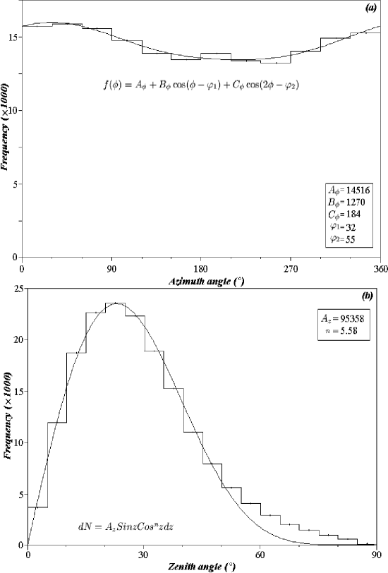
Figure 2: Local coordinates distributions of, (a) azimuth ’$\phi$’ and (b) zenith ’$z$’ angles of logged EAS events.

Fig. 2(a) shows the azimuthal angle distribution of the EAS events which is nearly isotropic. A slight North-South anisotropy is observed which is attributed to the geomagnetic field. We fitted this distribution with a harmonic function as follow : (Bahmanabadi et al. (2002))

$$\\ f(\phi)=A_{\phi}+B_{\phi}\cos(\phi-\varphi_{1})+C_{\phi}\cos(2\phi-\varphi_{2})$$ (14)

where A_ϕ, B_ϕ and C_ϕ are respectively 14516, 1270 and 184. $\varphi_{1}$ and $\varphi_{2}$ are phase constants which are respectively 32^∘ and 55^∘.
Since thickness of the atmosphere increases quickly with increasing zenith angle $z$ (Gaisser, T.K., (1990)), the number of EAS events is strongly related to the $z$ value, as shown in Fig. 2(b).
These distributions were studied separately for the two experimental configuration $E1$ and $E2$. The shower rate in $E2$ is less than $E1$ because of the larger size of the array in $E2$. However the zenith angle distributions in $E1$ and $E2$ are very similar. The differential zenith angle distributions of these data sets are fitted to the function $dN=A_{z}SinzCos^{n}zdz$ with a very good agreement for both $E1$ and $E2$ which from 0^∘ to 50^∘ $A_{z}=95358$ and $n=5.85$ and from 50^∘ to 60^∘ $A_{z}=90189$ and $n=5.00$. From another view the mean value of zenith angle $(\bar{z})$ is $26.2746$ and $26.4625$ in $E1$ and $E2$ respectively. Since the results of the two experimental configurations, are in a good agreement with one another and the excess is important for us. Therefore we added the two data sets to obtain a larger data set with lower energy threshold of $E1$ which is 39 TeV.

3.3 Calculation of equatorial and galactic coordinates of each EAS event

The equatorial coordinates (RA,Dec) are obtained from calculated local coordinates ($z,\varphi$), GMT of each EAS event and geographical latitude of the array. In this step the transformation relations (see http://aanda.u-strasbg.fr , Roy, A.E., & Clarke, D. ), and the local sidereal time of the starting point of the experiment (see http://tycho.usno.navy.mil/sidereal.html ) were used.
Then galactic coordinates (l,b) of each EAS event are obtained from the calculated equatorial coordinates, based on the galactic coordinate standard of year 2000 (see http://aanda.u-strasbg.fr ). Fig. 3 shows the distribution of our data in galactic coordinates.

3.4 Error estimation of investigated sources in galactic coordinates

For the coordinates calculations of each EAS event in galactic coordinates we have to know estimated errors in these coordinates. These errors are due to experimental error factors, which contain uncertainties in time and coordinates of each logged EAS event. The defined distance between two scintillators was centre to centre and the size of the scintillators were ($100\times 100\times 2$ cm³). Meanwhile the accuracy of coordinates of each scintillator is measured within a few centimeters. So error in measurement of coordinates of secondary particles of each EAS event is $\Delta d\cong 1$ m.
The errors in time measurement of each EAS event are due to the front thickness of the secondary particles, electronics errors and error in GMT logging. The error due to the first two factors was $\Delta t\cong 2$ns (Bahmanabadi et al. (2002)). The error in GMT logged time of each EAS event was $\Delta T=0.07$s which is due to recording rate and the synchronizing of the computer. These errors make uncertainties in galactic coordinates of the investigated sources by the array.
The following errors were calculated :

• The errors in local, equatorial and galactic coordinates of each EAS event.

• The observational angular error of each source.

• The mean and standard deviation of these error angles. We calculated these steps for more than 1000 random sources which are in the Field Of View (FOV) of the array. This calculation was carried out for $E1$ and $E2$ separately and was weighted by their refined EAS events.

From geometry of Fig. 1 we can drive :

$$\sin z\sin\varphi=\frac{c}{d}(t_{2}-t_{1})$$ (15)

$$\sin z\cos\varphi=\frac{c}{d}(t_{3}-t_{2})$$ (16)

In these relations $t_{i}$s are logged times of an EAS event in i_th component of the array and $d$ is side of the square array.
The errors in zenith and azimuth angles were obtained by differentiating from eqs. (5) and (6) :

$$\Delta z^{2}=A_{\Delta}^{2}/\cos^{2}z+B_{\Delta}^{2}\tan^{2}z$$ (17)

$$\Delta\varphi^{2}=A_{\Delta}^{2}/\sin^{2}z$$ (18)

where $A_{\Delta}=2c\Delta t/d$ and $B_{\Delta}=\Delta d/d$. The errors in equatorial and galactic coordinates were calculated from differentials of Dec(z,$\varphi$), RA(z,$\varphi,T$), b(RA,Dec) and l(RA,Dec).
If $y$ is a generic function of parameters $u$, $v$ and $T$, then :

$$y=y(u,v,T)\\$$ (19)

$$|\Delta y|=\sqrt{(\frac{dy}{du})^{2}\Delta u^{2}+(\frac{dy}{dv})^{2}\Delta v^{2}+(\frac{dy}{dT})^{2}\Delta T^{2}}$$ (20)

Where $dy/dT=2\alpha$ ($\alpha=1.00273790935$) (see http://tycho.usno.navy.mil/sidereal.html ) for the calculation of RA(z,$\varphi,T$) and $dy/dT=0$ for calculation of Dec(z,$\varphi$), b(RA,Dec) and l(RA,Dec).
The error on the observed solid angle of each source is $\Delta\Omega=\cos$b$\Delta$b$\Delta$l and the equivalent error on the angular radius is $r_{e}\cong\sqrt{\Delta\Omega/\pi}$ ($r_{e}\ll 1$)
The upper analysis obtains angular resolution of each EAS event individually. In case that there are many EAS events with different local coordinates which have contributions in the signature of each investigated source. Therefore at first angular errors of all of the accumulated EAS events in the galactic coordinates of the source were calculated, then the mean value of these angular errors was chosen as angular error of the source for the first step. Since all of the accumulated EAS events in the angular error region have contributions in the source signature, so the previous calculations were repeated for all of the accumulated EAS events in a circular region with the center of the source and radius of $r_{e}$. Finally the mean value of these EAS angular errors is calculated as angular error of each source in galactic coordinates. Since the side distances of the array is different in $E1$ and $E2$, angular errors in these two experiments are different. So for calculation of the final result for each source these angular errors calculated separately for $E1$ and $E2$ and was weighted with the number of refined EAS events in the related experiment. The final angular errors of investigated sources ($r_{e}$) are shown in Table 1. Since these angular error radii have a little fluctuations respect to their mean, therefore we sampled over l and b with a step of 5 degrees from the FOV of the array and calculated these radii to find the mean and standard deviation. Therefore the mean value and the standard deviation of the angular error of the experiment was obtained from angular error of more than 1000 random points. With These steps we obtained $\bar{r_{e}}=4.35^{\circ}\pm 0.82^{\circ}$ as the mean angular error of the experiment.

3.5 Drawing exposure map and simulation of the experiment

Because of the various exposures of the sky in time, there is a non-uniform distribution of EAS events in galactic coordinates. The variation in time exposures due to the altitude difference of different sources, and the observation of separate individual galactic regions during the sub-intervals within the long duration of the experiment were simulated. We have 166665 EAS events in our experiments, so we used monte carlo method for this simulation and we simulated 166665 random events. These random numbers were chosen with considerations of Fig. 2. From this figure is seen that $\phi$ distribution is not isotropic and the thickness effect of the atmosphere is very important, these effects were considered in choosing of these random numbers. So in the procedure :

• Zenith angle $(z)$ was taken from 1^∘ to 60^∘.

• Azimuth angle $(\phi)$ was chosen from 1^∘ to 360^∘.

• Related random numbers of time were chosen with consideration of EAS event rate of the experiment. Meanwhile we considered duration of the experiment which was taken from start and stop times of each sub-experiment.

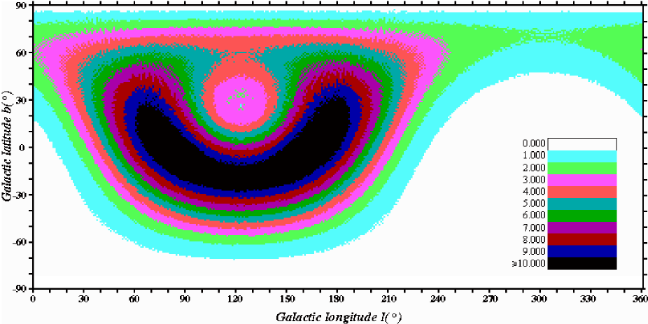
Figure 4: Exposure map of simulated events in 1${}^{\circ}\times$1^∘ bins base on the general parameters of total distribution of EAS events in galactic coordinates.

With this procedure we obtained 2500 simulated map and obtained the map with mean number of simulated events per ($1^{\circ}\times 1^{\circ}$) pixel with the accuracy of 0.001. Fig. 4 shows the exposure map of the experiment. The event map in Fig. 3 reflects the uneven exposure of the experiment.

3.6 Investigation of EGRET gamma-ray sources and measurement of their statistical significance

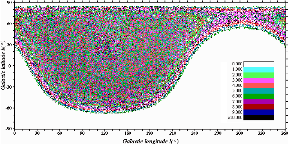
Figure 5: Corrected exposure map which is extracted from division of the data map (Fig. 3) to the exposure map (Fig. 4) pixel by pixel.

The energy range of the logged EAS events by the array is in the range of 40 to 10,000 TeV. In this energy range distribution of cosmic-rays is completely isotropic and homogeneous in the galaxy. After correcting for the exposure effects, we looked for excess emission that could be from gamma-ray sources. We used third EGRET catalogue (Hartman et al. (1999)) as a reference. But some of EGRET sources have not acceptable events in the FOV of our array. So we counted number of events, number of pixels and then calculated count per pixel related to each of these sources. We note that the mean count per pixel in data map is 4.798. Of 151 EGRET sources only 123 of them have count per pixel of more than square root of 4.798 with 98 more than 1.5 times the square root of the mean. So we started our investigations on these 98 sources. A method of excess similar to the analysis adopted by the Tibet EAS array, has been adopted (Amenomori et al. (2002) & tibet2000 (2000)). In the first step we divided the data map (Fig. 3) to the exposure map (Fig. 4) pixel by pixel. in the obtained map, approximately most of non zero pixels are around 1 except probable source pixels and pixels with more fluctuations in the data map, which probably due to the smallness of the data set. For eliminating the fluctuated pixels we multiplied the new map to 4.798 as raw exposure corrected map. In this step we added counts of all pixels of the raw corrected map. The number must be very near to 166,665 so with this restriction we obtained a lower limit 0.0750 for eliminating pixels with less count in the exposure map, and the final exposure corrected map was obtained which is shown in Fig. 5.
The obtained map was fairly uniform in the FOV of our array in the galactic coordinates. Next we investigated the remaining faint inhomogeneity in the corrected map that could be conditionally attributed to the existence of gamma-ray sources. To estimate the significance of an individual source we obtained all corrected EAS events, $N_{on}$, within a radius $\sqrt{2}r_{e}$from the source position. The number of pixels, $n_{s}$, within this region was also found. The total number of background counts, $N_{off}$, was found from the pixels that fall within an outer radius of 2$r_{e}$ and an inner radius $\sqrt{2}r_{e}$ from the source position. The number of background pixels, $n_{b}$, was also calculated. The statistical significance of the source was obtained using the Li & Ma relation (Li & Ma (1983)).

$$S=\frac{N_{on}-\alpha N_{off}}{\sqrt{N_{on}+\alpha^{2}N_{off}}}\hskip 14.22636pt,\hskip 14.22636pt\alpha=\frac{n_{s}}{n_{b}}$$ (21)

Distribution of statistical significance of these 98 sources is fitted on a gaussian function as follow :

$$f(\sigma)=a_{\sigma}exp(-\frac{(\sigma-b_{\sigma})^{2}}{2c_{\sigma}^{2}})$$ (22)

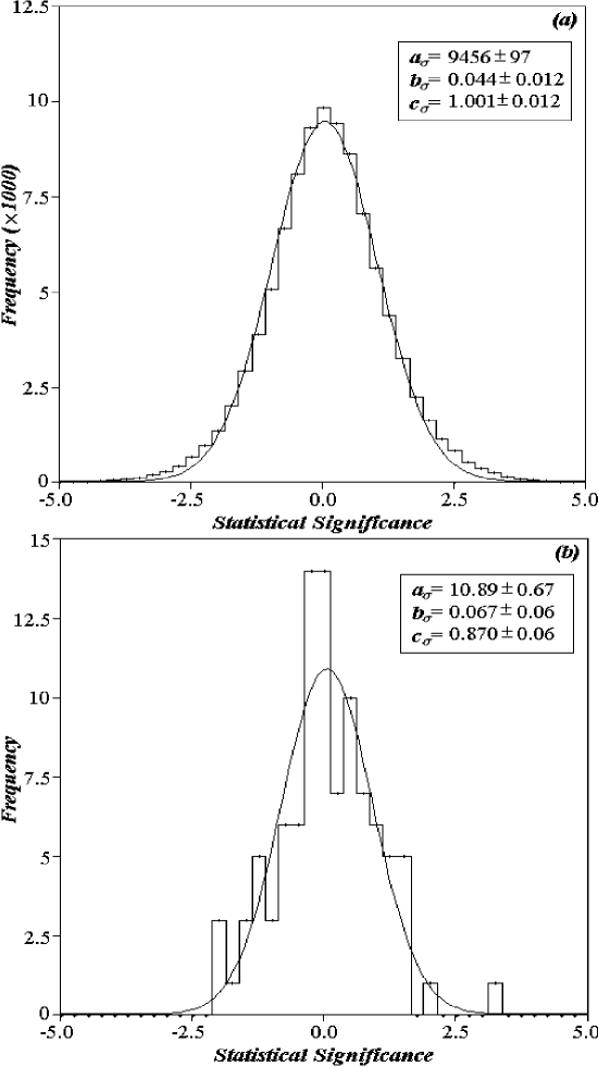
Figure 6: Distribution of frequency of (a) 98,000 virtual random sources and (b) 98 EGRET sources in the FOV of our array in galactic coordinates versus their statistical significance. a_σ, b_σ and c_σ are described in eq. (14)

which is shown in Fig. 6. Then for the investigation of the statistical significance distribution, we chose 98,000 virtual random sources with similar conditions of the 98 EGRET sources. Fig. 6 shows a normal distribution with mean 0.044 and standard deviation 1.001. Procedure of the significance calculation of these virtual sources is as like as the 98 EGRET sources except a little difference. Basically the virtual sources have no signals so we used another relation for the calculation of their statistical significance (Li & Ma (1983)).

$$S=\frac{N_{on}-\alpha N_{off}}{\sqrt{\alpha(N_{on}+N_{off})}}\hskip 14.22636pt,\hskip 14.22636pt\alpha=\frac{n_{s}}{n_{b}}$$ (23)

3.7 Investigation of a probable displacement of the source signatures

Our exposure corrected map has not any bright source signatures, so we used third EGRET catalogue as a reference for searching some sources in our energy range. But EGRET energy range is from 100 MeV to 30 GeV and our energy range is from 40 TeV to 10,000 TeV. So to search for some sources in our data we ought to hope that these sources have had a spread spectrum at least from EGRET energy range to our energy range, like blazars, BL Lac objects, Flat-spectrum radio quazars or etc. Since usually these sources in different ranges of energies have not the same places exactly and they have a little displacement, we searched around these sources with one degree displacement. This displaced l and b are shown in Table 1 for each source. It means that around each source with statistical significance more than 1 we tried 8 ($1^{\circ}\times 1^{\circ}$)pixels around it and chose the location with highest statistical significance.

4 Results

4.1 Explanation of the Field of View (FOV) in galactic coordinates

The rotation axis of the Earth passes near the star Polaris, angular difference between Polaris and the rotation axis is approximately 5 times smaller than our mean accuracy ($\bar{r_{e}}$) in galactic coordinates. So in this analysis Polaris is considered as being on the rotation axis of the Earth. The longitude and latitude of Polaris in galactic coordinates are $123^{\circ}$,$17^{{}^{\prime}}$ and $27^{\circ}$,$28^{{}^{\prime}}$ respectively. The geographical latitude of Tehran is $35^{\circ}$ $N$, so the angle between the zenith of the array and Polaris in Tehran is $55^{\circ}$, we selected events with zenith angles less than $60^{\circ}$ for the analysis which is deduced from Fig. 2(b) and therefore, Polaris and regions around it are observable only with High zenith EAS events. From Fig. 2(b) it can be seen that the best observable region is from $10^{\circ}$ to $40^{\circ}$ of zenith angles. In Fig. 3 is shown that Galactic longitudes smaller than $l\approx 123^{\circ}-(2\times 60^{\circ}-(60-55)^{\circ})\approx 8^{\circ}$ and larger than $l\approx 123^{\circ}+(2\times 60^{\circ}-5^{\circ})\approx 238^{\circ}$ are less observable. In other words, given the location of the array these are two different observable regions in galactic coordinates. Galactic latitudes smaller than $b\approx 27^{\circ}-(60^{\circ}-5^{\circ})\approx-38^{\circ}$ and larger than $b\approx 27^{\circ}+(60^{\circ}-5^{\circ})\approx 82^{\circ}$ are less observable regions too.

4.2 Comparison of observed sources of $E1$ and $E2$

With the procedure which is mentioned in subsection 3.7. we searched for sources with statistical significance more than 1.5, and we found thirteen sources which five of them are more than 2. For avoiding from probable fluctuations we did another try. we searched these displaced sources in $E1$ and $E2$ separately. But in this stage because of the smallness of these data sets, specially in $E1$ we separated significance more than 1. Therefore 10 sources remained which have statistical significance more than 1 in $E1$ and $E2$ and more than 1.5 in the sum, which are shown in Table 1. Fortunately five of these sources are AGNs, one is probably AGN and four of them are unidentified sources. This is in case that from 271 source of 3rd EGRET catalogue sources only 66 are AGNs.

4.3 Distribution of observed shower events around most significant EGRET sources

It seems that radial distribution of number of counts per pixel for each source naturally must be near to a gaussian distribution as a source signature, over a flat back ground. We separated eight regions with approximately the same number of pixels for each source. The first region is a circle with radius $\sqrt{1/2}r_{e}$. The second region is a ring with inner radius $\sqrt{1/2}r_{e}$ and outer radius $\sqrt{2/2}r_{e}$ and with this order we separated eight regions. Distribution of mean counts per pixel around 98,000 virtual random sources and 10 most significant EGRET sources is shown in Fig. 7. These distributions fitted on a gaussian function over a flat distribution as follow:

$$f(r_{e})=a_{r}+b_{r}exp(-r_{e}^{2}/2c_{r}^{2}).$$ (24)

5 Discussion and concluding remarks

In Table 1 is seen that most significant excesses observed, are in the region $15^{\circ}<\bar{z}<35^{\circ}$. This result is reasonable because these angles are in favorable locations in the sky and have considerably more data from this region. In addition our data have a few counts in some parts of Fig. 3 and we were mandated to eliminate some source candidates from our list. To increase the statistical significance of our results and investigation of more sources, we have to accumulate more data to have a map with less fluctuations.
There has been a considerable effort worldwide to detect gamma-ray sources via the EAS technique. From a variety of arguments we suspect that some, if not many, of the EGRET sources would be detectable at very high energies. In this work, we are limited to a discussion of a few sources with relatively small statistical significance. Our statistical significance are not in a detection limit with confident, we studied this procedure to guess some candidates in unidentified EGRET sources more than TeV range. For these sources listed in Table 1, we suspect that nine of them may be extra-galactic ($|b|>20^{\circ}$) (Gehrels et al. (2000)) and only one is in galactic region ($|b|\leq 20^{\circ}$) and this one is an AGN in the third EGRET catalogue list too. Four of our ten sources were investigated before with CASA-MIA (Catanese et al. (1996)) and two of them were GEV EGRET sources (Lamb & Macomb (1997)). Therefore we might expect that as many as four of these unidentified sources could indeed be emitters at high energy and might be AGNs.
Some of our observed sources overlap one another Fig. 8, so a complete and accurate analysis procedure would incorporate the maximum likelihood method (Mattox et al. (1996)). We must also emphasize that our experiment can not distinguish between gamma-ray and cosmic-ray initiated air showers, and so we used the excess method to carry out a search for very high energy gamma-ray emission. After the analysis we understood that the record times per second of our computer is very important and we have to increase this record rate to decrease angular error radius of observable sources. In our future site at 2600 m a.s.l. (see http://sina.sharif.edu/^∼observatory/ ), we are constructing underground tunnels which will provide us with ample space to deploy muon detectors. The detection of muons in air showers should be provide a powerful away to discriminate between cosmic-ray and gamma-ray air showers.

	Name	l	b	ID	ld	bd	$\sigma_{E1}$	$\sigma_{E2}$	$\sigma_{tot}$	$r_{e}(^{\circ})$	$\bar{z}$	Flux	t1	t2
1	3EG J0237+1635	156.46	-39.28	A	157	-39	1.29	2.80	2.90	4.70	24.87	630	$\surd$	$\surd$
2	3EG J0407+1710	175.63	-25.06		175	-24	1.65	1.28	1.95	4.78	24.05	782
3	3EG J0426+1333	181.98	-23.82		182	-23	1.11	2.60	2.79	4.89	26.97	702
4	3EG J0808+5114	167.51	32.66	a	168	33	1.40	1.37	1.91	5.10	23.29	1241
5	3EG J1104+3809	179.97	65.04	A	180	66	1.17	1.30	1.73	4.43	15.97	485	$\surd$	$\surd$
6	3EG J1308+8744	122.74	29.38		124	28	2.43	1.88	3.43	4.76	44.14	412
7	3EG J1608+1055	23.51	41.05	A	23	42	1.53	1.55	2.11	4.62	29.27	431	$\surd$
8	3EG J1824+3441	62.49	20.14		61	21	1.05	1.60	1.91	4.74	16.19	1370
9	3EG J2036+1132	56.12	-17.18	A	57	-18	1.09	1.62	1.95	5.16	28.05	851
10	3EG J2209+2401	81.83	-25.65	A	81	-27	1.45	1.60	1.86	4.25	21.40	844	$\surd$

Table 1: Observed EGRET 3rd catalogue sources by our array. l_d and b_d are displaced galactic coordinates, $\sigma_{E1}$, $\sigma_{E2}$ and $\sigma_{tot}$ are the statistical significance related to the first experiment, the second experiment and sum of both, $r_{e}$ is error angular radius, $\bar{z}$ is mean amount of zenith angles of EASs related to each source and ’Flux’ is number of EAS events related to each source. t1 is AGNs which is investigated by CASA-MIA before (Catanese et al. (1996)), t2 is sources with energy more than 1 GeV (Lamb & Macomb (1997)). Meanwhile sources number 5 and 7 are ’Mrk 421’ and ’4C +10.45’ respectively

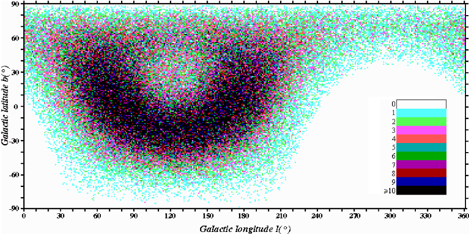
Figure 3: EAS events map in 1${}^{\circ}\times$1^∘ bin galactic coordinates.

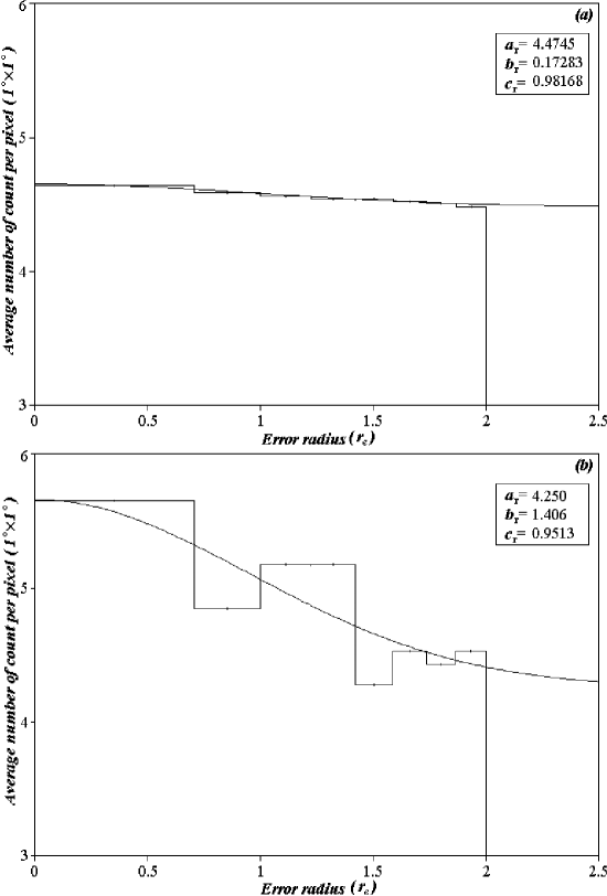
Figure 7: Distribution of mean count per pixel of (a) 98,000 virtual random sources and (b) 10 EGRET sources of Table 1 versus error radial distance from the centre of the related sources.

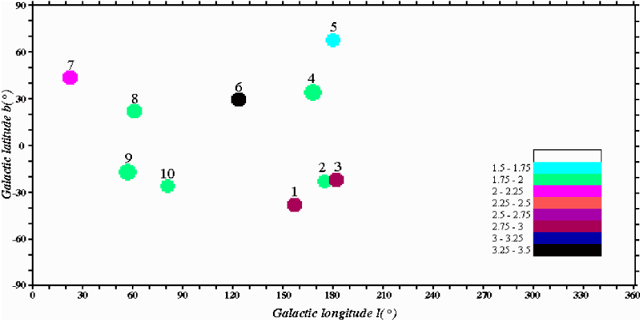
Figure 8: Map of EGRET sources with statistical significance more than 1.5 in galactic coordinates. The numbered sources were described in Table 1.

References

- Alexandreas et al. (1993) Alexandreas, D.E., et al., 1993, Ap.J., 405, 353
- Amenomori et al. (2002) Amenomori, M., et al. 2002, ApJ, 580, 887
- (3) Amenomori, M., et al. 2000, ApJ, 532, 302
- Bahmanabadi et al. (2003) Bahmanabadi, M., et al., 2003, Experimental Astronomy, 15(1), 13.
- Bahmanabadi et al. (2002) Bahmanabadi, M., et al., 2002, Experimental Astronomy, 13(1), 39.
- Bahmanabadi et al. (1998) Bahmanabadi, M., et al., 1998, Experimental Astronomy, 8(3), 211.
- Bahmanabadi et al. (1998) Bahmanabadi, M., et al., 1998, Ph.D. thesis, Sharif university, Tehran, Iran.
- Bhattacharya et al. (2003) Bhattacharya, D., Akyuz, A., Miyagi, T., Samimi, J. 2003, A&A, 404, 163
- Borione et al. (1997) Borione, A., et al., 1997, Ap.J., 481, 313
- Case & Bhattacharya (1998) Case, G.L., Bhattacharya, D. 1998, Ap.J., 504, 761
- Catanese et al. (1996) Catanese, M., et al. 1996, ApJ, 469, 572
- Colafrancesco, S., (2002) Colafrancesco, S., 2002, A&A, 396, 31
- Combi et al. (2001) Combi, J.A., Romero, G.E., Benaglia, P., Jonas, J.L. 2001, A&A, 366, 1047
- D’Amico et al. (2001) D’Amico, N., et al. 2001, A&A, 552, L45
- Dixon et al. (1998) Dixon, D.D., Hartmann, D.H., Kolaczik, E.D., Samimi, J. 1998, New Astron., 3, 539
- Gaisser, T.K., (1990) Gaisser, T.K., ’Cosmic Rars and Particle Physics’.
- Gehrels et al. (2000) Gehrels, N., et al. 2000 ,Nature , 404, 363
- Grainer (2000) Grainer, I.A. 2000, A&A, 364, L93
- Harding & Zhang (2001) Harding, A.K., Zhang, B. 2001, ApJ, 548, L37
- Hartman et al. (1999) Hartman, R.C., et al. 1999, ApJS., 123, 79
- (21) http://sina.sharif.edu/∼observatory/
- (22) http://aanda.u-strasbg.fr:2002/articles/astro/full/1998/01/ds1449/node3.html
- (23) http://www.timeanddate.com/worldclock/personalapplet.html
- (24) http://tycho.usno.navy.mil/sidereal.html
- Hunter et al. (1997) Hunter, S.D., et al. 1997, ApJ, 481, 205
- Lamb & Macomb (1997) Lamb, R.C., Macomb, D.J. 1997, ApJ, 488, 872
- Li & Ma (1983) Li, T., Ma, Y. 1983, ApJ, 272, 317
- Mattox et al. (1996) Mattox, J.R., et al. 1996, ApJ, 461, 396
- McKay et al. (1993) McKay, T.A., et al. 1993, ApJ, 417, 742
- Mitsui, K., et al. (1990) Mitsui, K., et al., 1990, Nucl. Inst. Meth., A223, 173
- Romero et al. (1999) Romero, G.E., Benaglia, P., Torres, D.F. 1999, A&A, 348, 868
- (32) Roy, A.E., and Clarke, D., ’Astronomy : Principle and Practice’.
- Sreekumar et al. (1998) Sreekumar, P., et al. 1998, ApJ, 494, 523
- Sturner & Dermer (1995) Sturner, S.J., Dermer, C.D. 1995, A&A, 293, L17
- Torres et al. (2003) Torres, D.F., Reucroft, S., Reimer, O., Anchordoqui, L.A., 2003, ApJ, 595, L13
- Torres et al. (2001) Torres, D.F., Butt, Y.M., Camilo, F. 2001, ApJ, 560, L155
- Zhang et al. (2000) Zhang, L., Zhang, Y.J., Cheng, K.S. 2000, A&A, 357, 957