Bayesian cross-validation by parallel Markov chain Monte Carlo

Abstract

Brute force cross-validation (CV) is a method for predictive assessment and model selection that is general and applicable to a wide range of Bayesian models. Naive or ‘brute force’ CV approaches are often too computationally costly for interactive modeling workflows, especially when inference relies on Markov chain Monte Carlo (MCMC). We propose overcoming this limitation using massively parallel MCMC. Using accelerator hardware such as graphics processor units (GPUs), our approach can be about as fast (in wall clock time) as a single full-data model fit.

Parallel CV is flexible because it can easily exploit a wide range data partitioning schemes, such as those designed for non-exchangeable data. It can also accommodate a range of scoring rules.

We propose MCMC diagnostics, including a summary of MCMC mixing based on the popular potential scale reduction factor ($\widehat{\mathrm{R}}$) and MCMC effective sample size ($\widehat{\mathrm{ESS}}$) measures. We also describe a method for determining whether an $\widehat{\mathrm{R}}$ diagnostic indicates approximate stationarity of the chains, that may be of more general interest for applications beyond parallel CV. Finally, we show that parallel CV and its diagnostics can be implemented with online algorithms, allowing parallel CV to scale up to very large blocking designs on memory-constrained computing accelerators.

1 Overview

Bayesian cross-validation [CV; 9, 46] is a method for assessing models’ predictive ability, and is a popular basis for model selection. Naive or ‘brute force’ approaches to CV, which repeatedly fits models to data subsets, are computationally demanding. Brute force CV is especially costly when the number of folds is large and inference is performed by Markov chain Monte Carlo (MCMC) sampling. Furthermore, since MCMC inference must be closely supervised to identify issues and to monitor convergence, assessing many models fits can also be labor-intensive. Consequently, brute force CV is often impractical under conventional inference workflows [e.g., 15].

Fast alternatives to brute force CV exist for special cases. Importance sampling and Pareto-smoothed importance sampling [11, 47] require only a single MCMC model fit to approximate leave-one-out (LOO) CV. However, importance sampling is known to fail when the resampling weights have thick-tailed distributions, which is especially likely for CV schemes designed for non-exchangeable data. Examples include $hv$-block CV for time series applications [36] and leave-one-group-out (LOGO) CV for grouped hierarchical models, where several observations are left out at the same time. In these cases, the analyst must fall back on brute force methods.

In this paper, we show that general brute force CV by MCMC is feasible on computing accelerator hardware, specifically on graphics processor units (GPUs). Our method, which we call parallel CV (PCV), includes an inference workflow and associated MCMC diagnostic methods. PCV is not a replacement for standard inference workflows, but rather an extension that applies after criticism of candidate models. PCV runs inference for all folds in parallel, potentially requiring thousands of independent MCMC chains, and assesses convergence across all chains simultaneously using diagnostic statistics that target the overall CV objective. Our experiments show that PCV can estimate moderately large CV problems on an ‘interactive’ timescale—that is, a similar elapsed wall clock time as the original full-data model fit by MCMC.

PCV is an application of massively parallel MCMC, which takes advantage of recent developments in hardware and software [see e.g. 28] and CV’s embarrassingly parallel nature. Unlike the ‘short chain’ parallel MCMC approach which targets a single posterior, we target multiple independent posteriors concurrently on a single computer. Other approaches include independent chains run on separate CPU cores and/or within-chain parallelism, both of which are available in the Stan language [45]. Local balancing approaches parallel inference by generating ‘clouds’ of proposals for each MCMC step [17, 8, 21]. [34] handle large datasets by targeting a single composite posterior with distributed MCMC samplers applied to different data subsets [see also 49, 41].

In addition to parallelism, PCV further reduces computational effort compared with naive brute force CV. First, PCV simplifies warm-up runs by reusing information generated during full-data inference, in effect exploiting the similarity between the full-data and partial-data CV posteriors. Second, running chains in parallel allows early termination as soon as the required accuracy is achieved. Since Monte Carlo (MC) uncertainty is usually small relative to the irreducible CV epistemic uncertainty (see section 2.2), applications of CV for model selection typically require only relatively short MCMC runs. The third way is technical, and applies where online algorithms are used. These have small, stable working sets and make effective use of memory caches on modern computer architectures [see e.g. 35, 44], although we do not analyze this phenomenon in this paper.

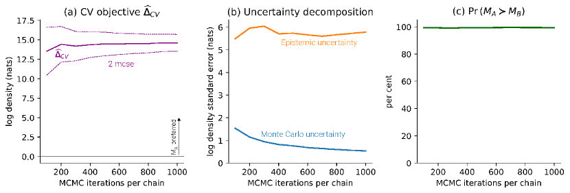
Figure 1: Model selection for a leave-one-group-out CV (LOGO-CV) for a toy hierarchical Gaussian regression problem, using the log score (Example 1). Model $M_{A}$ is correctly specified, including all 4 regressors, while $M_{B}$ is misspecified and includes only 3. MCMC inference uses 4 chains per fold, for a total of 200 chains. Panel (a) shows the score difference $\widehat{\Delta}$ and 2 Monte Carlo standard error (MCSE) interval as a function of MCMC iterations per chain. Positive (negative) score values favor $M_{A}$ ($M_{B}$). Panel (b) shows that epistemic uncertainty dominates MC uncertainty, demonstrating the limited utility of further reducing MC uncertainty. Panel (c) shows that $\Pr\left(M_{A}\succ M_{B}\,|\,y\right)$ quickly stabilizes close to 100%. See Section 2.1 for full details.

Figure 1 previews a PCV model selection application for a hierarchical Gaussian regression model, described in Section 2.1. The goal of this exercise is to estimate the probability that one model predicts better than another under the logarithmic scoring rule and a LOGO-CV design. The results clearly stabilize after just a few hundred MCMC iterations. This is explained by the fact that the MC uncertainty is small relative to epistemic uncertainty, so that running the MCMC algorithm for longer confers little additional insight.

In summary, this paper makes the following contributions to a methodological toolkit for parallel CV:

• A practical workflow for fast, general brute force CV on computing accelerators (Section 3);

• A massively parallel sampler and associated diagnostics for PCV, including online estimators for all estimators and diagnostics discussed in this paper (Section 3.3); and

• A measure of MC and epistemic uncertainty [43], the effective sample size ($\widehat{\mathrm{ESS}}$; [37]), and a measure of mixing based on the $\widehat{\mathrm{R}}$ statistic [13, 48] (Section 4).

• Examples with accompanying software implementations (Section 5 and supplement).

2 Background

This section provides a brief overview of predictive model assessment and MCMC-based Bayesian inference. Consider an observed data vector $y\sim p_{\mathrm{true}}$, where $p_{\mathrm{true}}$ denotes some ‘correct’ but unknown joint data distribution. Suppose an analyst fits some Bayesian model $M$ for the purpose of predicting unseen realizations $\tilde{y}$ from $p_{\mathrm{true}}$. Having fit the posterior distribution $p\left(\theta\,|\,y,M\right)$, the predictive density $f_{M}$ is a posterior-weighted mixture,

$$f_{M,y}\left(\tilde{y}\right)=\int p_{y}\left(\tilde{y}\,|\,\theta,M\right)p\left(\theta\,|\,y,M\right)d\theta.$$ (1)

With the predictive $f_{M,y}$ in hand, two natural question arise. First, how well does $f_{M,y}$ predict unseen observations (out of sample)? Second, if multiple models are available, which one predicts better?

2.1 Predictive assessment

If the true data distribution $p_{\mathrm{true}}\left(\tilde{y}\right)$ were somehow known, one could assess the predictive performance of $f_{M,y}$ directly using a scoring rule. A scoring rule $S\left(q,y\right)$ is a functional that maps a predictive density $q$ and a realization $y$ to a numerical assessment of that prediction. A natural summary of the performance of $f_{M,y}$ is the expected score,

$$S_{M,y}=\int p_{\mathrm{true}}\left(\tilde{y}\right)S\left(f_{M,y},\tilde{y}\right)\,\mathrm{d}\tilde{y}.$$ (2)

Furthermore, it is straightforward to use $S_{M,y}$ as a basis for model selection. For a pairwise model comparison between candidate models, say $M_{A}$ and $M_{B}$, a simple decision rule relies only on the sign of the difference

$$\Delta=S_{M_{A},y}-S_{M_{B},y}.$$ (3)

Positive values of $\Delta$ indicate $M_{A}$ is preferred to $M_{B}$ under $S$, (an event we denote $M_{A}\succ M_{B}$) and vice-versa.

Ideally, the choice of scoring rule would be tailored to the application at hand. However, in the absence of an application-driven loss function, generic scoring rules are available. By far the most commonly-used scoring rule is the log predictive density $\mathrm{LogS}\left(f,y\right):=\log f(y)$, which has the desirable mathematical properties of being local and strictly proper [18]. $\mathrm{LogS}$ also has deep connections to the statistical concepts of KL divergence and entropy [see, e.g., 4]. While we focus on $\mathrm{LogS}$, it is worth noting that $\mathrm{LogS}$ has drawbacks too: it requires stronger theoretical conditions to reliably estimate scores using sampling methods and can encounter problems with models fit using improper priors [5]. More stable results can be obtained by alternative scoring rules, albeit at the cost of statistical power [25]. To demonstrate the flexibility of PCV in Appendix A we briefly discuss the use of alternative scoring rules, the Dawid-Sebastini score ($\mathrm{DSS}$; 6) and Hyvärinen score ($\mathrm{HS}$; 23).

Throughout the paper, we illustrate ideas using the following example, with results in Figure 1.

Example 1 (Model selection for a grouped Gaussian regression).

Consider the following regression model of grouped data:

$$y_{ij}\,|\,\alpha_{j},\beta,\sigma_{y}^{2}\overset{ind}{\sim}\mathcal{N}(\alpha_{j}+x_{j[i]}^{\top}\beta,\sigma_{y}^{2}),$$ (4)

for $i=1,\dots,N_{j},\quad j=1,\dots,J.$ The group effect prior is hierarchical,

$$\alpha_{j}|\mu_{\alpha},\sigma_{\alpha}^{2}\overset{iid}{\sim}\mathcal{N}(\mu_{\alpha},\sigma_{\alpha}^{2}),\quad j=1,\dots,J,$$ (5)

where $\mu_{\alpha}\sim\mathcal{N}\!(0,1)$ and $\sigma_{\alpha}\sim\mathcal{N}^{+}\!(0,10)$, the half-normal distribution with variance 10 and positive support. The remaining priors are $\sigma_{y}\sim\mathcal{N}^{+}\!(0,10)$ and $\beta\sim\mathcal{N}\!(0,I)$. Consider two candidate models distinguished by their group-wise explanatory variables $x_{j}$. Model $M_{A}$ is correctly, while model $M_{B}$ is missing one covariate. To assess an observation $\tilde{y}$ from group $j^{\prime}$ with explanatory variables $\tilde{x}_{j^{\prime}}$ with respect to $\mathrm{LogS}$, the predictive density is

$$f_{M,y}\left(\tilde{y}\right) =\int\mathcal{N}\!\left(\tilde{y}\,|\,\alpha_{j^{\prime}}+\tilde{x}_{j^{\prime}}^{\top}\beta,\sigma_{y}^{2}\right)p\left(\alpha_{j^{\prime}}\,|\,y,M\right)$$

$$\qquad p\left(\beta,\sigma_{y}^{2}\,|\,y,M\right)d\alpha_{j^{\prime}}\,d\beta\,d\sigma_{y}^{2}.$$ (6)

Here and for the remainder of the paper, $\mathcal{N}\!\left(x\,|\,\mu,\sigma^{2}\right)$ denotes the density of $\mathcal{N}\!\left(\mu,\sigma^{2}\right)$ evaluated at $x$. In the case where group $j^{\prime}$ does not appear in the training data vector $y$, the marginal posterior density $p\left(\alpha_{j^{\prime}}\,|\,y,M\right)$ that appears in (6) is defined using the posterior distributions for $\mu_{\alpha}$ and $\sigma_{\alpha}$, as

$$\int p\left(\alpha_{j^{\prime}}|\mu_{\alpha},\sigma_{\alpha}\right)p\left(\mu_{\alpha},\sigma_{\alpha}\,|\,y,M\right)d\mu_{\alpha}d\sigma_{\alpha}.$$ (7)

We simulate $J=50$ groups with $N_{j}=5$ observations per group. The elements of the $J\times 4$ matrix $X$ is simulated using $\mathcal{N}(0,10)$ variates. The true values of $\alpha$, $\beta$ and $\sigma^{2}$ used in the simulation are drawn from the priors. We use $L=4$ chains and $K=J=50$ folds, a total of 200 chains.

2.2 Cross-validation

In practice the true process $p_{\mathrm{true}}\left(\tilde{y}\right)$ is not known, so (2) cannot be computed directly. Rather, CV approximates (2) using only the observed data $y$ instead of future data $\tilde{y}$. CV proceeds by repeatedly fitting models to data subsets, assessing the resulting model predictions on left-out data. A CV scheme includes the choice of scoring rule and a data partitioning scheme that divides into pairs of mutually disjoint test and training sets $\left(\mathsf{test}_{k},\mathsf{train}_{k}\right)$, for $k=1,\dots,K$. The resulting partial-data posteriors $p\left(\cdot\,|\,y_{\mathsf{train}_{k}},M\right)$ can be viewed as $K$ random perturbations of the full-data posterior $p\left(\cdot\,|\,y,M\right)$.

Popular CV schemes include leave-one-out (LOO-CV) which drops a single observation each fold, and $K$-fold which divides the data into $K$ disjoint subsets. However, for non-exchangeable data, CV schemes often need to be tailored to the underlying structure of the data, or to the question at hand. For example, time-series, spatial, and spatio-temporal applications can benefit from specifically tailored partitioning schemes [see e.g., 38, 2, 30]. For some data structures the resulting $K$ can be particularly large, such as for LOO-CV and $h(v)$-block CV.

There may be several appropriate CV schemes for a given candidate model and dataset. The CV scheme should also reflect the nature of the generalization required. For example, in hierarchical models with group effects (Example 1), LOGO-CV measures the model’s ability to generalize to unseen data groups, while non-groupwise schemes applied to the same model and data would characterize predictive ability for the current set of groups only.

We focus on two CV objectives. First, the CV score $\widehat{S}_{M}$ is an estimate of predictive ability $S_{M}$. It is constructed as a sum over all $K$ folds,

$$\widehat{S}_{M}=\sum_{k=1}^{K}S\left(f_{M,k},y_{\mathsf{test}_{k}}\right),$$ (8)

where $f_{M,k}$ denotes the model $M$ predictive constructed using the posterior $p\left(\theta\,|\,y_{\mathsf{train}_{k}}\right)$. The quantity $\widehat{S}_{M}$ can be viewed as a Monte Carlo estimate of $S_{M}$, up to a scaling factor. Second, a CV estimate for the model selection objective $\Delta$ in (3) is the sum of the $K$ differences,

$$\widehat{\Delta} :=\widehat{S}_{M_{A}}-\widehat{S}_{M_{B}}$$

$$=\sum_{k=1}^{K}\left[S\left(f_{M_{A},k},y_{\mathsf{test}_{k}}\right)-S\left(f_{M_{B},k},y_{\mathsf{test}_{k}}\right)\right]$$

$$=:\sum_{k=1}^{K}\widehat{\Delta}_{k}.$$ (9)

Herein we use the generic notation $\widehat{\eta}=\sum_{k=1}^{K}\widehat{\eta}_{k}$ to denote the CV objective, whether it be $\widehat{S}_{M}$ or $\widehat{\Delta}$.

2.3 Epistemic uncertainty

The MC estimators in (8) and (9) are random quantities that are subject to sampling variability. The associated predictive assessments of out-of-sample model performance are therefore subject to uncertainty [43]. Naturally, there would be no uncertainty at all if $p_{\mathrm{true}}$ were fully known or if an infinitely large dataset were available. But since (8) and (9) are estimated from finite data, an assessment of the uncertainty of these predictions is useful for interpreting CV results [43, §2.2]. We call this random error epistemic uncertainty.

It can be helpful to view as-yet-unseen data as missing data. CV imputes that missing data with finite number of left-out observations. The epistemic uncertainty about the unseen future data can be regarded as uncertainty from the imputation process.

For a given dataset, epistemic uncertainty is irreducible in the sense that it cannot be driven to zero by additional computational effort or the use of more accurate inference methods. This contrasts with Monte Carlo uncertainty in MCMC inference, discussed in the next subsection. The limiting factor is the information in the available dataset.

We adopt the following popular approach to modeling epistemic uncertainty. First, we regard the individual contributions $\left(\widehat{\eta}_{k}\right)$ to $\widehat{\eta}$ as exchangeable, drawn from a large population with finite variance [46, 43]. That is, we presume that $K$ is reasonably large. Then, $\widehat{\eta}$ will satisfy a central limit theorem (CLT) so that a normal approximation for the out-of-sample predictive performance of $\widehat{\eta}$ is appropriate.

In particular, for model selection applications we are interested in the probability that $M_{A}$ predicts better than $M_{B}$, which we denote $\Pr\left(M_{A}\succ M_{B}\,|\,y\right)$. We approximate

$$\Pr\left(M_{A}\succ M_{B}\,|\,y\right)\approx\Phi\left(\frac{\widehat{\Delta}}{\sqrt{K\widehat{\sigma}_{\widehat{\Delta}}^{2}}}\right),$$ (10)

where $\widehat{\sigma}_{\widehat{\Delta}}^{2}=\frac{1}{K-1}\sum_{k=1}^{K}\left(\widehat{\Delta}_{k}-\widehat{\Delta}/K\right)^{2}$ is the sample variance of the contributions to (9) and $\Phi$ denotes the standard normal cdf.

There are other ways to model $\Pr\left(M_{A}\succ M_{B}\,|\,y\right)$, such as the Bayesian Bootstrap [40, 43]. We prefer the normal approximation in this setting because it performs well [43] and is simple to approximate with online estimators, making it particularly useful on parallel hardware.

2.4 MCMC inference

MCMC is by far the dominant method for conducting Bayesian inference. It characterizes posterior distributions with samples from a stationary Markov chain, for which the invariant distribution is the target posterior. MCMC sampling algorithms are initialized with a starting parameter value $\theta^{\left(0\right)}$, usually in a region of relatively high posterior density. Then, an MCMC algorithm is used to sequentially draw a sample $\theta^{\left(1\right)},\theta^{\left(2\right)},\dots$ from the chain. This sample can be used to construct Monte Carlo estimators for functionals $g\!\left(\theta\right)$ such as the predictive density $f_{M,y}\!\left(\tilde{y}\right)$ that appears in (1). Many MCMC algorithms are available: Gelman et al [14] provide a general overview.

For brute-force CV applications, posteriors are separately estimated for each model and fold. Furthermore, typical inference workflows for MCMC inference call for draws from $L>1$ independent chains targeting the same posterior. For model $M$, fold $k$, and chain $\ell$, denote the sequence of $N$ MCMC parameter draws $\theta_{M,k,\ell}^{\left(0\right)},\theta_{M,k,\ell}^{\left(1\right)},\cdots,\theta_{M,k,\ell}^{\left(N\right)}$, so that the expectation $\mathbb{E}\left[g\left(\theta\right)\,|\,M,y_{\mathsf{train}_{k}}\right]$ can be estimated for each model $M$ and fold $k$ as

$$\widehat{g}_{M,k}^{\left(N\right)}=\frac{1}{LN}\sum_{\ell=1}^{L}\sum_{n=1}^{N}g\left(\theta_{M,k,\ell}^{\left(n\right)}\right).$$ (11)

The main assumption needed is quite standard (see e.g. 24): a CLT for $\widehat{g}_{M,k}^{\left(N\right)}$, so that

$$\sqrt{N}\left(\widehat{g}_{M,k}^{\left(N\right)}-\mathbb{E}\left[g\left(\theta\right)\,|\,M,y_{\mathsf{train}_{k}}\right]\right)$$

$$\qquad\qquad\overset{d}{\longrightarrow}\mathcal{N}\left(0,\frac{\sigma_{\widehat{g}_{M,k}}^{2}}{L}\right)\ \text{as}\ N\to\infty.$$ (12)

Because MCMC parameter draws are auto-correlated, a naive estimate of the uncertainty associated with (11) from these draws will be biased. Instead, a Monte Carlo standard error (MCSE) estimator should be used. We use MCSE estimators based on batch means [24] because these can be efficiently implemented on accelerator hardware (see Appendix A). Let the chain length be a whole number representing $a$ batches each of $b$ samples, so that $N=ab$. Then the $h$th batch mean is given by

$$\bar{g}_{M,k,\ell}^{\left(h\right)}=\frac{1}{b}\sum_{n=\left(h-1\right)b+1}^{hb}g\left(\theta_{M,k,\ell}^{\left(n\right)}\right).$$ (13)

The MCSE $\sigma_{\hat{g}_{M,k}}/\sqrt{LN}$ can then be computed using the sample variance of the $\bar{g}_{M,k,\ell}^{\left(h\right)}$s across all $L$ chains for model $M$ and fold $k$, where

$$\hat{\sigma}_{\widehat{g}_{M,k}}^{2}=\frac{b}{La-1}\sum_{\ell=1}^{L}\sum_{h=1}^{a}\left(\bar{g}_{M,k,\ell}^{\left(h\right)}-\widehat{g}_{M,k}^{\left(N\right)}\right)^{2}.$$ (14)

There is a large literature on estimators for $\sigma_{\widehat{g}_{M,k}}^{2}$, but we use (14) since it is simple and it performed well in our experiments. The batch size $b$ is a hyper-parameter to be chosen before inference starts, and large enough for the $Y_{k}$ to be approximately independent. Where the MCMC chain length is known (in the case where a data-dependent stopping rule is not used), asymptotic arguments suggest $b=\left\lfloor\sqrt{NL}\right\rfloor$, for which a rough guess can be made a priori (see for instance 24 for a discussion).

To reliably fit Bayesian models, the inference workflow needs to include careful verification of model fit. MCMC algorithms must also be carefully checked for pathological behaviors and monitored for convergence so that inference can be terminated [15]. Most workflows are oriented toward parameter inference, ensuring that the samples adequately characterize the desired posterior distribution $p\left(\theta\,|\,y\right)$. Assessing convergence effectively amounts to verifying that (a) each posterior’s chains are correctly mixing, and (b) the sample size is large enough to characterize the posterior distribution to the desired degree of accuracy. To support these assessments, several diagnostic statistics are available [39]. We describe two diagnostic statistics specifically adapted for parallel MCMC in Section 4.

3 Parallel cross-validation

In this section we describe the proposed PCV workflow. PCV aims to make brute force CV feasible by reducing computation (wall clock) time as well as the analyst’s time spent checking diagnostics. Of course, given unlimited computing power and effort, an analyst could simply implement Bayesian CV by sequentially fitting each CV fold using MCMC, checking convergence statistics for each, then constructing the objective $\widehat{\eta}$ using (8) or (9). This is computationally and practically infeasible for CV designs with large $K$.

Many existing applications of massively parallel MCMC target just a single posterior. In contrast, PCV simultaneously estimates multiple posteriors using parallel samplers that execute in lock-step. Under our approach, the algorithm draws vectors of combined parameter vectors representing all chains for all folds. Estimating $\hat{\eta}$ by brute force MCMC requires samples from $\mathcal{O}\left(KL\right)$ parallel independent MCMC chains. In some cases, posteriors for different models can be sampled in parallel, too (see Appendix B).

The main challenge that must be solved for estimating all $K$ posteriors (or $2K$ posteriors for a pairwise model comparison) is that model criticism, diagnostics, and convergence checking must be applied to all posteriors under test. However, since full model criticism and checking should be performed on the full-data models anyway, for which the partial-data posteriors are simply random perturbations, we argue that model criticism need only be applied to the full-data candidate models. Furthermore, we can sharply reduce the computational effort required for sampling by using information from full-data inference to initialize the partial-data inference (Section 3.1).

We propose the following extension to conventional Bayesian inference workflows:

• Full-data model criticism and inference. Perform model criticism on candidate model(s) using the full data set [15], revising candidate models as necessary, and obtain MCMC posterior draws for each model;

• Parallel MCMC warmup (see Section 3.1). Initialize $L$ parallel chains for each of $K$ folds using random draws from the full-data MCMC draws obtained in Step 1. Run short warm-up chains in parallel and discard the output;

• Parallel sampling. Run the $\mathcal{O}(KL)$ parallel MCMC chains for $N$ iterations, accumulating statistics required to evaluate $\widehat{\eta}$ and associated uncertainty measures (see Section 3.2); and

• Check convergence. Compute and check parallel inference diagnostics (Section 4), and if necessary adjust inference settings and repeat.

3.1 Efficient MCMC warmup

General-purpose MCMC sampling procedures typically begin with a warmup phase. The warmup serves two goals: (i) it reduces MCMC estimator bias due to initialization, and (ii) adapts tuning parameters of the sampler. Warm-up procedures aim to ensure the distribution of the initial chain values $\theta_{\ell}^{(0)}$ is close to that of the target posterior. An example is Stan’s window adaptation algorithm [45], designed for samplers from the Hamiltonian Monte Carlo [HMC; 33] family. Hyperparameter choices are algorithm-specific: for example, HMC requires a step size, trajectory length, and inverse mass matrix.

The warm-up phase is computationally costly. It would be especially costly and time consuming to run complete, independent tuning procedures for each fold in parallel to obtain kernel hyperparameters and initial conditions $\mathcal{O}\left(KL\right)$ for each fold. In addition, running many independent tuning procedures can be unreliable. Tuning procedures are stochastic in nature, and as the number of chains increases, the probability of initializing at least one chain with problematic starting conditions increases. An example of such a starting condition is a parameter draw far in a region of the parameter space that leads to numerical problems and a ‘stuck chain’.

Instead of running independent warm-up procedures for each fold, we propose re-using the warm-up results from the full-data model for each CV fold, under the assumption that the full-data and partial-data posteriors are close. This assumption seems reasonable if the folds are similar enough to the full-data model for CV to be interpretable as a predictive assessment of the full-data model (Section 2.2).

Under this approach, each fold’s MCMC kernel uses the same inference tuning parameters (e.g. step size and trajectory length) as the full-data model. Starting positions are randomly drawn from the full-data posterior MCMC sample. To ensure distribution of the starting conditions are close to the fold model’s posterior distribution, PCV then simulates and discards a very short warm-up sample.

3.2 Estimating uncertainty

Practical CV applications require estimates of the uncertainty of $\widehat{\eta}$ estimates. Both MC and epistemic uncertainty contribute to the variability in $\widehat{\eta}$.

We estimate epistemic uncertainty by applying the normal approximation described in Section 2.3. For model selection application, we substitute fold-level estimates $\left(\widehat{\Delta}_{k}\right)$ into (10).

MC uncertainty can be estimated using an extension of standard methods described in Section 2.4. Because each fold is estimated using independent MCMC runs, the overall MC uncertainty for $\widehat{\eta}$ is simply the sum of the MC variance of each fold’s contribution. When an estimated scoring rule may be represented as a smooth function of an ergodic mean (like $\mathrm{LogS}$), $\sigma_{\hat{\eta}}^{2}$ can be estimated using the delta method. In the case of $\mathrm{LogS}$, we have

$$\sigma_{\hat{\eta}}^{2}=\sum_{M\in\mathcal{M}}\sum_{k=1}^{K}\sigma_{S_{M,k}}^{2}\approx\sum_{M\in\mathcal{M}}\sum_{k=1}^{K}\frac{\sigma_{\hat{f}_{M,k}}^{2}}{\left(\hat{f}_{M,k}\right)^{2}},$$ (15)

where summation over models reflects the fact that the MC error for a difference is the sum of the error for both terms. The MCSE for $\hat{\eta}$ is then $\mathrm{MCSE}_{\hat{\eta}}=\sigma_{\hat{\eta}}/\sqrt{LN}.$ Independence of the contributions to the overall MC error is helpful for producing accurate estimates quickly.

Even when $\eta$ and its associated standard error can theoretically be estimated using MC estimators (for instance if its first two moments are finite), in practice theoretical conditions may not be enough to prevent numerical problems during inference. A common cause of numerical overflow is the presence of outliers that fall far in the tails of predictive distributions.

In model selection applications, it is typical for MC uncertainty to be an order of magnitude smaller than epistemic uncertainty (see e.g. Figure 1). This discrepancy implies that, provided that the chains have mixed, long MCMC runs are not usually necessary in model selection applications, since additional effort applied to MCMC sampling will not meaningfully improve the accuracy of $\widehat{\eta}$. An overall measure that provides a single picture of uncertainty is also useful because the MCMC efficiency of individual folds can vary tremendously (see Section 4.1 and Figure 2).

Since PCV applications typically require only relatively small $N$ to make MC uncertainty insignificant compared to epistemic uncertainty, we do not propose a stopping rule for of the type discussed by Jones et al [24]. In most cases these rules are justified by asymptotic arguments (i.e. for large $N$), whereas in our examples $N$ is on the order of $10^{3}$.

3.3 Implementation on accelerator hardware

Massively parallel samplers are able to take advantage of modern computing accelerators, which can offer thousands of compute units per device. Accelerators typically offer more cost-effective throughput, measured in floating-point operations per second (FLOPS), than conventional CPU-based workstations. However, despite their impressive parallel computing throughput and cost per FLOPS, the design of computing accelerators impose heavy restrictions on the design of inference algorithms.

Programs with heavy control flow beyond standard linear algebra operations tend to be inefficient, including those commonly used in Bayesian inference such as sorting large data vectors. In addition, accelerators have limited onboard memory for storing and manipulating draws generated by MCMC samplers. The need to transfer MCMC draws to main memory for diagnostics and manipulation would represent a significant performance penalty. These problems could be alleviated if all analysis steps could be conducted on the accelerator device, within its memory limits.

The Hamiltonian Monte Carlo [HMC; 33] sampling algorithm lends itself well to implementation on accelerator hardware. To implement PCV, we augment the HMC kernel with an additional parameter representing the fold identifier. This allows the unnormalized log joint density—and its gradient via automatic differentiation—to select the appropriate data subsets for each chain. HMC is suitable for parallel operations because its integrator follows a fixed trajectory length at each MCMC iteration. The lack of a dynamic trajectory allows HMC to be vectorized across a large number of parallel chains, with each evolving in lock-step. In contrast, efficient parallel sampling is extremely difficult with dynamic algorithms such as the popular No-U-Turn Sampler [NUTS; 20]. Assessing chain efficiency (Section 4.1) is more important with samplers with non-adaptive step size like HMC, since samples tend to be more strongly auto-correlated than for adaptive methods, delivering fewer effective draws per iteration.

A further constraint inherent to computing accelerators is the size of the device’s on-board memory. Limited accelerator memory means it is usually infeasible to store all MCMC parameter draws from all chains for later analysis, which requires only $\mathcal{O}\left(KLN\dim\left(\theta\right)\right)$ memory. This cost can be prohibitive, especially when $\dim\left(\theta\right)$ is large. However, it is often feasible to store draws required to construct the objective, that is the univariate draws required to estimate $\hat{\eta}$, reducing the memory requirement to $\mathcal{O}\left(KLN\right)$. This approach is very simple to implement (see Algorithm 1).

Where accelerator device memory is so constrained that even the draws for $\hat{\eta}$ cannot be stored on the accelerator, online algorithms are available. The memory footprint for such algorithms does not depend on the chain length $N$. However, as Algorithm A2 in the supplementary material demonstrates, the fully-online approach is significantly more complicated. (See also the sampler implemented in Appendix D in the supplementary material.) While the online approach is very memory efficient, it is also less flexible. Conventional workflows recommend first running inference then computing diagnostics from the resulting draws. However, under the online approach one must predetermine which diagnostics will be run after inference, then accumulate enough information during inference to compute those diagnostics without reference to the full set of predictive draws (see Appendix A).

Posterior draws $\left\{\theta^{(\mathrm{fd})}_{1},\dots,\theta^{(\mathrm{fd})}_{N_{\mathrm{fd}}}\right\}$, MCMC kernels $\left\{\mathcal{T}_{k}\left(\theta,\cdot\right)\right\}_{k=1}^{K}$, log predictive densities $\left\{\log p\left(\tilde{y}_{k}\,|\,\theta\right)\right\}_{k=1}^{K}$, folds $K$, chains $L$, warm-up length $N_{\mathrm{wu}}$, chain length $N$

$\hat{s}$.

Initialize:

      $K\times L\times N$ array $\hat{s}$

for $k\in 1,\dots,K$ do in parallel: $\triangleright$ fold loop

    for $\ell\in 1,\dots,L$ do in parallel: $\triangleright$ chain loop

       $\theta^{(k,\ell)}\leftarrow\text{draw from }\left\{\theta^{(\mathrm{fd})}_{1},\dots,\theta^{(\mathrm{fd})}_{N_{\mathrm{fd}}}\right\}$

       for $i\in 1,\dots,N_{\mathrm{wu}}$ do sequentially $\triangleright$ warm-up sampling loop

          $\theta^{(k,\ell)}\leftarrow\text{draw from }\mathcal{T}_{k}\left(\theta^{(k,\ell)},\cdot\right)$

       end for

       for $i\in 1,\dots,N$ do sequentially $\triangleright$ sampling loop

          $\theta^{(k,\ell)}\leftarrow\text{draw from }\mathcal{T}_{k}\left(\theta^{(k,\ell)},\cdot\right)$

          $\hat{s}^{(k,\ell,i)}\leftarrow\log p\left(\tilde{y}_{k}\,|\,\theta^{(k,\ell)}\right)$

       end for

    end for

end for

Algorithm 1 Non-online parallel CV sampler for LogS. Superscripts index array elements. See also Algorithm A2 in the supplementary material.

4 MCMC diagnostics

We propose that diagnostics focus on $\widehat{\eta}$ rather than fold-specific parameters. Under our proposed workflow, the analyst will have completed model criticism on the full-data model before attempting brute force CV. Soundness of the full-data model strongly suggests that the CV folds, which by construction have the same model structure and similar data, will also behave well. However, inference of all folds should nonetheless be monitored to ensure convergence has been reached, and to identify common problems that may arise during computation.

A focus on the predictive quantity $\hat{\eta}$ rather than the model parameters carries several advantages. First, it provides a single view of convergence that targets the desired output and ignores any inference problems in irrelevant parts of the model, such as group-level random effects that are not required to predict the group of interest. Second, unlike parameter convergence diagnostics, diagnostics for $\hat{\eta}$ are sensitive to numerical issues arising in the predictive components of the model. Third, these diagnostics can be significantly cheaper to compute than whole-parameter diagnostics, in part because the target is univariate or low-dimensional.

Other diagnostic statistics for massively parallel inference include $\mathfrak{n}\widehat{R}$ [31], which is applicable to large numbers of short chains targeting the same posterior. In contrast, our diagnostics target a small number of longer chains per fold, and are applied to a large number of different posteriors.

4.1 Effective sample size

An (estimated) effective sample size ($\widehat{\mathrm{ESS}}$; 16) provides a scale-free measure of the information content of an autocorrelated sample. Since MCMC samples from a single chain are not independent, an estimate of the limiting variance $\sigma^{2}_{\hat{g}}$ in (12), denoted by $\widehat{\sigma}^{2}_{g}$, is typically greater than the usual sample variance $s_{g}^{2}$, and hence the degree of autocorrelation must be taken into account when computing the Monte Carlo standard error (MCSE) of estimates computed from the resulting MCMC sample.

The standard ESS measure targets individual parameter estimates, say $\theta_{i}$. Define $\widehat{\mathrm{ESS}}_{\theta_{i}}$, as the raw sample size adjusted by the ratio of the unadjusted sample variance $s^{2}_{\theta_{i}}$ to the corresponding MC variance $\hat{\sigma}_{\theta_{i}}^{2}$: $\widehat{\mathrm{ESS}}_{\theta_{i}}=LNs_{\theta_{i}}^{2}/\hat{\sigma}_{\theta_{i}}^{2}.$ For parallel inference we use the batch means method described in Section 2.4 to estimate $\hat{\sigma}_{\theta_{i}}^{2}$, for which online estimators are simple to implement. (For alternatives see e.g., the review by 39.)

For PCV, an aggregate measure of the sample size $\widehat{\mathrm{ESS}}$ can be computed similarly. Define $\widehat{\mathrm{ESS}}=LNs_{\hat{\eta}}^{2}/\hat{\sigma}_{\hat{\eta}}^{2}$. $\widehat{\mathrm{ESS}}$ is useful as a single scale-free measure across all folds (see Figure 2).

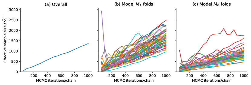
Figure 2: Progressive estimated effective sample size ($\widehat{\mathrm{ESS}}$) for Example 1 (grouped Gaussian regression), a scale-free measure of information content for the MCMC sample, as a function of MCMC iterations. Panel (a) shows $\widehat{\mathrm{ESS}}$ for the overall model selection statistic (incorporating all chains), while panels (b) and (c) respectively show the $\widehat{\mathrm{ESS}}$ for each fold of models $M_{A}$ and $M_{B}$. Note the overall measure falls within the range of all folds.

4.2 Mixing: aggregate $\widehat{R}_{\mathrm{max}}$

To assess mixing of the ensemble of chains, we propose a combined measure of mixing based on the potential scale reduction factor $\widehat{\mathrm{R}}$ [13, 48]. Most of the chains in the ensemble should have $\widehat{R}$s below a suitable threshold (Vehtari et al [48] suggest 1.01). In addition, we assess overall chain convergence by $\widehat{R}_{\mathrm{max}}$, the maximum of the $\widehat{\mathrm{R}}$s measured across all folds. Below, we describe a simple problem-specific method for interpreting $\widehat{R}_{\mathrm{max}}$.

The canonical $\widehat{\mathrm{R}}$ measure aims to assess whether the independent chains targeting the same posterior adequately characterize the whole posterior distribution. $\widehat{R}$ usually targets parameter means, but in our experiments we found that the mean of the log score draws to be a useful $\widehat{R}$ target. Other targets are of course possible, and wide range of other functionals appear in the literature [e.g. 48, 32].

$\widehat{\mathrm{R}}$ is a scaled measure of the variance of between-chain means $B$, a quantity that should decrease to zero as the chains converge in distribution and become more similar. Several variants of $\widehat{\mathrm{R}}$ exist. To simplify computation on accelerators, the simple version we use here omits chain splitting and rank-normalization (these features are described by 48). For a given model $M$ and fold $k$, define $\widehat{\mathrm{R}}$ as

$$\widehat{\mathrm{R}}_{M,k}=\sqrt{\frac{\frac{N-1}{N}\widehat{W}_{M,k}+\frac{1}{N}\widehat{B}_{M,k}}{\widehat{W}_{M,k}}}.$$ (16)

The within-chain variance $W_{M,k}$ and between-chain variance $B_{M,k}$ are, respectively

$$W_{M,k} =\frac{1}{L}\sum_{\ell=1}^{L}\frac{1}{N-1}\sum_{n=1}^{N}\left(\hat{s}_{M,k,\ell}^{\left(n\right)}-\bar{s}_{M,k,\ell}\right)^{2},$$

$$B_{M,k} =\frac{N}{L-1}\sum_{\ell=1}^{L}\left(\bar{s}_{M,k,\ell}-\bar{s}_{M,k,\cdot}\right)^{2},$$

where $\hat{s}_{M,k,\ell}^{\left(n\right)}$ is the $n$th draw of $\log p(\tilde{y}|\theta)$ in chain $\ell$, $\bar{s}_{M,k,\ell}$ is the chain sample mean, and $\bar{s}_{M,k,\cdot}$ is the sample mean of parameter draws for the fold $k$ chains.

The summary mixing measure is then

$$\widehat{R}_{\mathrm{max}}=\max_{M\in\mathcal{M},k=1,\dots,K}\widehat{R}_{M,k}.$$ (17)

Since all the $\widehat{\mathrm{R}}_{M,k}$ tend to 1 as chains converge and $K$ is fixed, it follows that $\widehat{R}_{\mathrm{max}}$ tends to 1 as all posterior chains converge.

However, while $\hat{R}_{\max}$ has the same limiting value as $\widehat{\mathrm{R}}$, it is not at all clear that the broadly accepted threshold of $\widehat{\mathrm{R}}<1.01$ [48] for a single posterior is an appropriate indicator that all folds have fully mixed. Each $\widehat{\mathrm{R}}_{M,k}$ is a stochastic quantity, and the extremum statistic $\widehat{R}_{\mathrm{max}}$ is likely to be large relative to the majority of chains.

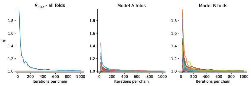
Figure 3: Progressive $\widehat{\mathrm{R}}$ measures as a function of iterations/chain for the toy grouped regression model comparison. Note that the 1.01 threshold [48] is exceeded by at least one chain, and hence by $\widehat{R}_{\mathrm{max}}$, for most of the 1,000 iterations/chain plotted in this diagram.

Figure 3 compares $\widehat{R}_{\mathrm{max}}$ with the $\widehat{\mathrm{R}}$ computed for each fold of both regression models $M_{A}$ and $M_{B}$. Recall from Figure 1 that that the $\widehat{\eta}$ estimates stabilize after a few hundred MCMC iterations per chain. However, well beyond this point, $\widehat{R}_{\mathrm{max}}$ exceeds the conventional convergence threshold for $\widehat{\mathrm{R}}$ of 1.01 [48].

To estimate an appropriate benchmark for $\widehat{R}_{\mathrm{max}}$ for a given problem, we propose the following simulation-based procedure. This procedure empirically accounts for the autocorrelation in each chain, without the need to model the behavior of each fold’s posterior, and with only minimal additional computation. This approach is conceptually similar to the block bootstrap, and it directly accounts for the autocorrelation in each fold’s MCMC chains.

Suppose (hypothetically) that all chains are well-mixed, so that the mean and variance of any chain should be roughly the same. In that case, if we also assume that autocorrelation is close to zero within the block size, then computing $\widehat{\mathrm{R}}$ should not be greatly affected if blocks of each chains are ‘shuffled’ as shown in Panel (a) of Figure 4. To construct an estimate of the likely range of $\widehat{\mathrm{R}}$ values under the assumption that the chains have mixed, we simply repeatedly compute $\widehat{\mathrm{R}}$ from a large sample of shuffled draws. Rather than adopt a threshold based on an arbitrary summary statistic of the shuffled draws as a single benchmark (say an upper quantile), we instead simply present the draws as a histogram for visual comparison.

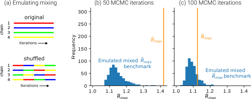
Figure 4: Two values of $\widehat{R}_{\mathrm{max}}$ for the toy regression problem, compared with emulated mixed $\widehat{R}_{\mathrm{max}}$ benchmark draws, computed by block-shuffling chains. Panel (a) shows a stylized shuffling scheme, where chains are broken into contiguous blocks and recombined by shuffling with replacement. Panels (b) and (c) show $\widehat{R}_{\mathrm{max}}$ estimates at 50 and 100 parallel MCMC iterations, respectively (vertical line), alongside histograms of 500 shuffled $\widehat{R}_{\mathrm{max}}$ draws for comparison. 5 blocks were used. In this example, we conclude that the parallel chains have not converged after 50 iterations, but they have after 100.

Figure 5 demonstrates $\widehat{R}_{\mathrm{max}}$ detecting two artificially-created pathological conditions: a stuck chain and a shifted chain, both of which correspond to non-convergence of one of the folds. To be clear, we do not claim that this $\widehat{R}_{\mathrm{max}}$ benchmark is foolproof or even that it will detect most convergence issues, but it did perform well in our examples when the bulk of folds had mixed (Section 5).

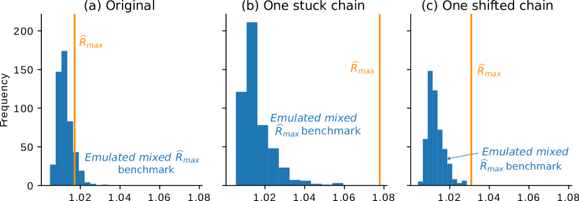
Figure 5: Artificially constructed pathological inference examples, detected by $\widehat{R}_{\mathrm{max}}$. Panel (a) shows the original comparison in Figure 4, after 1,000 iterations. In Panel (b) a single chain for one of the folds has been fixed to a constant value (its first draw). In Panel (c) a single chain for one of the folds has been shifted by 5 units. In both panels (b) and (c), $\widehat{R}_{\mathrm{max}}$ lies to the right of the histogram of 100 emulated stationary $\widehat{R}_{\mathrm{max}}$ draws, estimated using 5 blocks.

5 Illustrative examples

In this section we present three additional applied examples of PCV. Each example uses PCV to select between two candidate models for a given application. Code can be found online at https://github.com/kuperov/ParallelCV. For each candidate model, we first perform model checking on the full-data model prior to running CV, where chains are initialized using prior draws. For all experiments, we fix the batch size $b=50$, and check that this batch size yields reasonable ESS estimates compared with window methods [26] on the full-data models.

The core procedure we use for our experiments requires only a log joint likelihood function and log predictive density function compatible with JAX’s primitives, and is therefore amenable to automatic vectorization. Our examples use the HMC and window adaptation implementations in Blackjax v1.0 [27], as well as primitives in TensorFlow Probability (TFP; [7]). All experiments use double-precision (64-bit) arithmetic. Full-data inference is performed on the CPU while parallel inference is run on the GPU. CPU and GPU details are noted in each results table.

Example 2 (Rat weight).

This example demonstrates PCV on grouped data. Gelfand et al [10] present a model of the weight of $J=30$ rats, for each of which five weight measurements are available. The rat weights are modeled as a function of time,

$$M_{A}: y_{j,t}|\alpha_{j},\beta_{j},\sigma_{y} \sim\mathcal{N}\left(\alpha_{j}+\beta_{j}t,\sigma^{2}_{y}\right),$$ (18)

for $j=1,\dots,J;t\in\left\{8,15,22,29,36\right\}$, where $\alpha_{j}$ and $\beta_{j}$ denote random effects per rat. The model $M_{A}$ random effects and per-rat effects are modeled hierarchically,

$$\alpha_{j}\,|\,\mu_{\alpha},\sigma_{\alpha}\sim\mathcal{N}\left(\mu_{\alpha},\sigma_{\alpha}^{2}\right),\hfill\beta_{j}\sim\mathcal{N}\left(\mu_{\beta},\sigma_{\beta}^{2}\right)$$ (19)

with hyper-priors $\mu_{\alpha}\sim\mathcal{N}\left(250,20\right)$, $\mu_{\beta}\sim\mathcal{N}\left(6,2\right)$, $\sigma_{\alpha}\sim\mathrm{Gamma}\left(25,2\right)$, and $\sigma_{\beta}\sim\mathrm{Gamma}\left(5,10\right)$. The observation noise prior is $\sigma_{y}\sim\mathrm{Gamma}(1,2)$. Prior parameters were chosen using prior predictive checks.

In this example, we use parallel CV to check whether the random effect (i.e. rat-specific slope $\beta_{j}$) does a better job of predicting the weight of a new rat, than if a common $\beta$ had been used. The CV scheme leaves a rat out for each fold, for a total of $K=30$ folds. The alternative model is

$$M_{B}:y_{j,t}|\alpha_{j},\beta,\sigma^{2}\sim\mathcal{N}\left(\alpha_{j}+\beta t,\sigma^{2}\right),$$ (20)

for $j=1,\dots,J;t\in\left\{8,15,22,29,36\right\}$, where the prior $\beta\sim\mathcal{N}\left(6,2\right)$ was chosen using prior predictive checks [14].

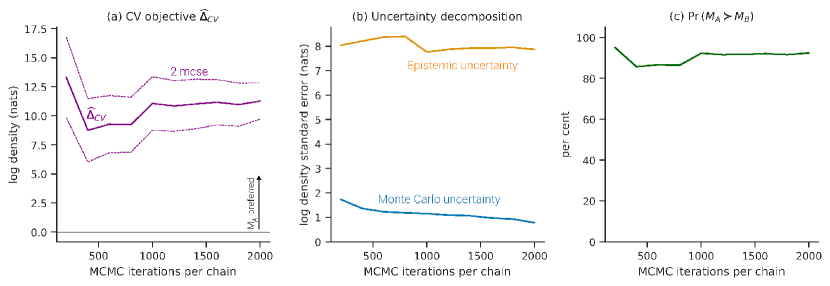
Figure 6: Progressive estimates for groupwise cross-validation for Example 2 (rat weight). The model selection statistic $\widehat{\Delta}$ shown in Panel (a) is clearly positive, favoring model $M_{A}$. Panel (b) shows that MC uncertainty is a very small component of the total. Panel (c) shows that the probability of $M_{A}$ predicting better than $M_{B}$ stabilizes after about 1,000 iterations.

Figure 6 shows that the PCV results have stabilized by 1,000 iterations, and $\Pr\left(M_{A}\succ M_{B}\right)\approx 90\%$. On an NVIDIA T4 GPU, PCV with 480 chains targeting all 60 posteriors took 18 seconds, which included a 10 second warm-up phase (Table C2 in Appendix C). Full-data inference took 11 and 15 seconds, respectively, which suggests naive brute force CV would take about 13 minutes. $\widehat{R}_{\mathrm{max}}$ plots suggest convergence after around 500 iterations per chain (Figure C2, Appendix C). In contrast, many chains still exceeded the 1.01 benchmark for $\widehat{\mathrm{R}}$ even after $2,000$ iterations (Figure C1, Appendix C).

Example 3 (Home radon).

Radon is a naturally-occurring radioactive element that is known to cause lung cancer in patients exposed to sufficiently high concentrations. Gelman and Hill [12] present a hierarchical model of radon concentrations in U.S. homes. The data cover $N_{D}=12,573$ homes in $J=386$ counties. For our purposes we will assume that the goal of the model is to predict the level of radon in U.S. counties, including those not in the sample (i.e. out-of-sample county-wise prediction). The authors model the level of radon $y_{i}$ in the $i$th house as normal, conditional on a random county effect $\alpha_{j}$ and the floor of the house $x_{i}$ where the measurement was taken. We will compare two model formulations:

$$M_{A}: y_{i}\,|\,\alpha,\beta,\sigma_{y}^{2} \sim\mathcal{N}\left(\alpha_{j\left[i\right]}+\beta x_{i},\sigma_{y}^{2}\right),$$ (21)

$$M_{B}: y_{i}\,|\,\alpha,\beta,\sigma_{y}^{2} \sim\mathcal{N}\left(\alpha_{j\left[i\right]},\sigma_{y}^{2}\right),$$ (22)

for $i=1,\dots,N_{D},$, where $\beta$ is a fixed effect, $\alpha_{j\left[i\right]}$ is the random effect for the county corresponding to observation $i$, and $\sigma^{2}$ is a common observation variance. For both models the county effect is modeled hierarchically,

$$\alpha_{j}\,|\,\mu_{\alpha},\sigma_{\alpha}^{2}\sim\mathcal{N}\left(\mu_{\alpha},\sigma_{\alpha}^{2}\right),$$ (23)

for $j=1,\dots,J$. The remaining priors are chosen to be weakly informative, $\mu_{\alpha}\sim\mathcal{N}\left(0,4\right)$ and $\sigma_{\alpha}^{2}\sim\mathrm{Gamma}\left(6,9\right)$. The other parameter priors are $\beta\sim\mathcal{N}\left(0,1\right)$ and $\sigma_{y}^{2}\sim\mathrm{Gamma}\left(10,10\right)$. A non-centered parameterization is used for MCMC inference and the model is fit by HMC. Prior parameters were chosen using prior predictive checks.

We will use county-wise PCV to determine whether the floor measure improves predictive performance. The estimate $\Pr\left(M_{A}\succ M_{B}\right)\approx 100\%$ stabilizes quickly (Figure 7).

The parallel inference procedure takes a total of 92 seconds to draw 2,000 parallel MCMC iterations plus 2,000 warmup iterations across a total of 3,088 chains targeting 772 posteriors. The 386 fold posteriors are sampled consecutively for each model. This compares with 45 and 35 seconds for the full-data models (see Table C3 in Appendix C for details). At 35 seconds per fold, a naive implementation of brute force CV across all would have taken 7.5 hours to run.

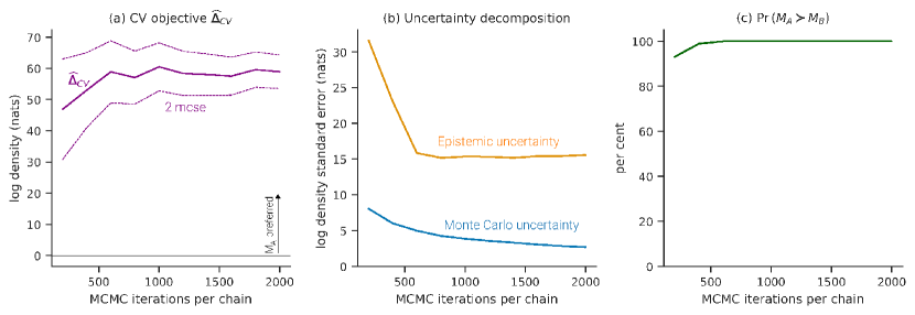
Figure 7: Progressive estimates for groupwise cross-validation for Example 3 (home radon). Model $M_{A}$ is preferred. The model selection statistic (a) is clearly positive and the probability that $M_{A}$ predicts better than $M_{B}$ stabilizes within a few hundred iterations.

Example 4 (Air passenger traffic to Australia).

Australia is an island nation, for which almost all migration is by air travel. Models of passenger arrivals and departures are useful for estimating airport service requirements, the health of the tourist sector, and economic growth resulting from immigration.

We compare two simple models of monthly international air arrivals to all Australian airports in the period 1985-2019, using data provided by the Australian Bureau of Transport and Infrastructure Research Economic (BITRE). The data are seasonal and nonstationary (Figure C5, Appendix C), so we model month-on-month ($M_{A}$) and year-on-year ($M_{B}$) changes with a seasonal autoregression. The power spectrum of the month/month growth rates display seasonality at several frequencies, while annual figures do not, suggesting that annual seasonality is present (Figure C6, Appendix C).

It is therefore natural to model these series using seasonal autoregressions on the month/month or year/year growth rates. Let $y_{t}\in\mathbb{R}$ denote the growth rate, observed monthly. We model

$$y_{t}=\sum_{i=1}^{p}\rho_{i}y_{t-i}+\beta_{0}+\sum_{j=1}^{q}\beta_{j}d_{j}+\sigma\varepsilon_{t},$$ (24)

for $t=1,\dots,T,\quad\varepsilon_{t}\overset{\mathrm{iid}}{\sim}\mathcal{N}\left(0,1\right).$. The noise standard deviation prior is $\sigma\sim\mathcal{N}^{+}\left(0,1\right)$. For AR effects we impose the prior $\left(2\rho_{i}-1\right)\sim\mathrm{Beta}\left(5,5\right)$ and for the constant and seasonal effects $\beta_{j}\sim\mathcal{N}\left(0,1\right)$.

Parallel CV results stabilize after a few hundred iterations per chain (Figure C4, Appendix C). PCV took a total of 6.1 seconds to draw to draw 500 iterations per chain (Table C4, Appendix C). Naively running all 790 models in succession would have taken about 4.4 hours.

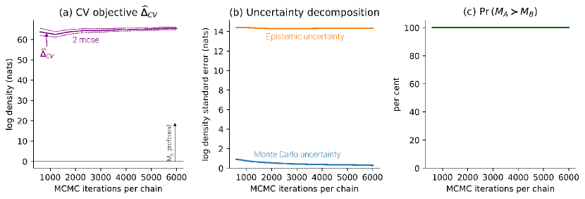
Figure 8: Progressive estimates for groupwise cross-validation for Example 4, the model of passenger arrivals. The model selection statistic (a) is clearly positive and the probability of $M_{A}$ predicting better than $M_{B}$ stabilizes within a few hundred iterations.

6 Discussion

We have demonstrated a practical workflow for conducting fast, general brute force CV in parallel on modern computing accelerator hardware. We have also contributed methods for implementing and checking the resulting output.

Our proposed workflow is a natural extension of standard Bayesian inference workflows for MCMC-based inference [15], extended to include initialization of parallel MCMC chains and joint convergence assessment for the overall CV objective.

The use of parallel hardware enables significantly faster CV procedures (in wall clock time), and on a practical level represents a sharp improvement in both flexibility and speed over existing CPU-based approaches. In contrast to approximate CV methods, our approach reflects a transition from computing environments that are predominantly compute-bound (where storage and bandwidth are not practically constrained), to a new era with fewer constraints on computing power but where memory and bandwidth are more limited. Efficient use of parallel hardware can in some cases reduce the energy required and associated carbon release for compute-heavy tasks, such as simulation studies involving repeated applications of CV.

Our proposed diagnostic criteria provide the analyst with tools for assessing convergence across a large number of estimated posteriors, alleviating the need to examine each posterior individually. Further efficiencies could be gained by developing formal stopping rules for halting inference when chains have mixed and the desired accuracy has been attained, although stopping rules should be applied with care as they can also increase bias [e.g., 24, 3]. We leave this to future research.

Moreover, online algorithms’ frugal memory requirements carries advantages for several classes of users. Top-end GPUs can run larger models (and/or more folds simultaneously), while commodity computers (e.g. laptops with less capable integrated GPUs) can perform a larger range of useful tasks. Beyond accelerator hardware, our approach may have benefits on CPU-based architectures too, by exploiting within-core vector units and possibly improving processor cache performance because of the tight memory footprint of online samplers.

Two possible extensions to this work could further reduce memory footprint on accelerators. The adaptive subsampling approach of Magnusson et al [29] would require that only a subset of folds be estimated before a decision became clear. In addition, the use of stochastic HMC [1] would permit that only a subset of the dataset be loaded on the accelerator at any one time.

Further work could include adaptive methods to focus computational effort in the areas that would most benefit from further MCMC draws, for example on fold posteriors with the largest MC variance, as well as a stopping rule to halt inference when a decision is clear. Turn-key parallel brute-force CV routines would be a useful natural extension to probabilistic programming languages. Parallel CV can also be done using inference methods other than MCMC, such as variational inference.

Acknowledgments

The authors would like to thank Charles Margossian for helpful comments. AC’s work was supported in part by an Australian Government Research Training Program Scholarship. AV acknowledges the Research Council of Finland Flagship program: Finnish Center for Artificial Intelligence, and Academy of Finland project (340721). CF acknowledges financial support under National Science Foundation Grant SES-1921523.

Appendix A Online parallel CV algorithms

Scoring rules that can be represented as functions of ergodic averages of the chains can also be implemented with a online estimator. Specifically, we require that we can express

$$\widehat{S}\left(p\left(\tilde{y}\,|\,y\right),\tilde{y}\right)\equiv\phi\left(\hat{\mu},\hat{\Sigma}\right)\qquad$$ (25)

where $\phi:\mathbb{R}^{d}\times\mathbb{R}^{d\times d}\to\mathbb{R}$ and $\xi:\Theta\to\mathbb{R}^{d}$ are functions, and

$$\hat{\mu}=\frac{1}{S}\sum_{s=1}^{S}\xi\left(\theta^{(s)}\right)\quad\text{and}\quad\hat{\Sigma}=\frac{1}{S-1}\sum_{s=1}^{S}\left[\xi\left(\theta^{(s)}\right)-\hat{\mu}\right]\left[\xi\left(\theta^{(s)}\right)-\hat{\mu}\right]^{\top}.$$ (26)

Scoring rules of this form include $\mathrm{LogS}$, $\mathrm{DSS}$, and $\mathrm{HS}$ (Table 1). Local scoring rules require only $\hat{\mu}$.

More general scoring rules, including the popular continuous ranked probability score (CRPS; 18) cannot easily be implemented with online algorithms as they typically require a full set of draws to be saved to the accelerator during inference for post processing. In addition, a need for constant memory precludes the use of many popular diagnostics, such as trace plots.

A.1 Online variance estimators

Estimating $\widehat{\eta}$ and MCMC diagnostics requires estimates for means and variances of sequences of values, computed without reference the full history of draws produced during inference. Computing the mean and variance of a sequence $x_{1},\dots,x_{N}$ without retaining individual values can be achieved using the method of Welford [51].

Consider first the univariate case. We sequentially accumulate the sum $x_{1}+x_{2}+\dots$ in the scalar variable $A_{x}$ and sum of squares $x_{1}^{2}+x_{2}^{2}+\dots$ in $A_{x^{2}}$. Then the mean $\bar{x}=A_{x}/N$ and

$$\operatorname{var}(x)=\frac{1}{N-1}\sum_{i=1}^{N}\left(x_{i}-\bar{x}\right)^{2}=\frac{1}{N-1}\left(A_{x^{2}}-\frac{A_{x}^{2}}{N}\right).$$ (27)

In the vector case, we accumulate the sum in $A_{x}$ and sum of outer squares in $A_{xx^{\top}}$. We will also ‘center’ these estimates as follows. Let $C\in\mathbb{R}^{d}$ be an estimate of the mean $\bar{x}$, where $d=\mathrm{dim}(\bar{x})$. We will accumulate the sequence of statistics $A_{x}^{(i)}$ and $A_{xx^{\top}}^{({i})}$ by each iteration evaluating the recursions

$$A_{x}^{(i)}=A_{x}^{(i-1)}+\left(x_{i}-C\right),\qquad A_{xx^{\top}}^{(i)}=A_{xx^{\top}}^{(i-1)}+\left(x_{i}-C\right)\left(x_{i}-C\right)^{\top},$$ (28)

with $A_{x}^{(0)}=A_{xx^{\top}}^{(0)}=0$. The role of the centering constant $C$ is to ensure that the accumulated values do not grow too large, leading to numerical overflow. We only need to allocate memory for a single $d$-vector $A_{x}^{(i)}$ and $d\times d$ matrix $A_{xx^{\top}}^{(i)}$. The mean is given by $\bar{x}=A_{x}^{(N)}/N+C$, and the covariance can be computed as

$$\mathrm{cov}\left(x\right) =\frac{1}{N-1}\sum_{j=1}^{N}\left(x_{j}-C+C-\bar{x}\right)\left(x_{j}-C+C-\bar{x}\right)^{\top}$$ (29)

$$=\frac{1}{N-1}\left[A_{xx^{\top}}^{(N)}-\frac{1}{N}A_{x}^{(N)}\left(A_{x}^{(N)}\right)^{\top}\right].$$ (30)

To compute the covariance of batch means of size $a\in\mathbb{N}$, replace $x_{i}$ with the $j$th batch mean $\bar{x}_{j}$ and evaluate the recursions (28) every $a$ iterations.

To stabilize these calculations for small values like probability densities, we store values in logarithms to avoid numerical underflow (e.g. $U_{x}=\log A_{x}$). Increments of the form (28) should use the numerically stable logsumexp function, available on most platforms. The need to take care to ensure numerical stability is especially acute on computing accelerators where lower-precision arithmetic (e.g. 32-bit or even 16-bit floats) is often preferred for increased performance.

Objective	Function $\phi$	Function $\xi$
	$\left(\hat{\mu},\hat{\Sigma}\right)\mapsto$	$\theta^{\left(s\right)}\mapsto$
LogS	$\log\left(\hat{\mu}\right)$	$p\left(\tilde{y}\,|\,\theta^{\left(s\right)}\right)$
HS	$-2\hat{\mu}_{1}+\hat{\mu}_{2}^{2}$	$\begin{bmatrix}\frac{\partial^{2}\log p\left(\tilde{y}_{i}\,|\,\theta^{\left(s\right)}\right)}{\partial\tilde{y}_{i}^{2}}+\left(\frac{\partial\log p\left(\tilde{y}_{i}\,|\,\theta^{\left(s\right)}\right)}{\partial\tilde{y}_{i}}\right)^{2}\\ \frac{\partial\log p\left(\tilde{y}_{i}\,|\,\theta^{\left(s\right)}\right)}{\partial\tilde{y}_{i}}\end{bmatrix}$
DSS	$\begin{array}[]{c}-\log\left|\hat{\Sigma}\right|\\ -\left(y-\hat{\mu}\right)^{\top}\hat{\Sigma}^{-1}\left(y-\hat{\mu}\right)\end{array}$	indep. draw from $p\left(\tilde{y}\,|\,\theta^{\left(s\right)}\right)$

Table 1: Functions for constructing online estimators of three positively-oriented scoring rules: logarithmic score (LogS), Hyvärinen score (HS), and Dawid-Sebastini score (DSS). The estimated score $\phi:\mathbb{R}^{d}\times\mathbb{R}^{d\times d}\to\mathbb{R}$ is a function of $\hat{\mu}$ and $\hat{\Sigma}$, respectively the sample mean and variance of $\left\{\xi\left(\theta^{(s)}\right):\,s=1,\dots,S\right\}$, where $\xi:\Theta\to\mathbb{R}^{d}$ is a function of individual MCMC parameter draws. For simplicity, this table drops CV fold indexes from the notation.

A.2 Logarithmic score (LogS)

Algorithm 2 details a online PCV sampler for a single model. This sampler can serve as a building block for (say) conducting pairwise model assessment. A sample python implementation can be found in Appendix E2.

The sampler operates on all folds and chains in parallel. Within each chain, the sampler first runs a warmup loop (see Section 3). In the main inference loop is divided into a nested hierarchy of MCMC batches and shuffle blocks. The arrays $U_{x}$ and $U_{x^{2}}$ accumulate the log sum of predictive densities and corresponding sum of squares for each fold and chain, respectively. Similarly, $V_{x}$ and $V_{x^{2}}$ accumulate the same for batch means, with one increment per batch loop. Each MCMC step, the arrays $Y_{x}$ and $Y_{x^{2}}$ accumulate the sum of centered log densities and squared log densities, respectively, which are required to compute $\widehat{\mathrm{R}}$. $Y_{x}$ and $Y_{x^{2}}$ are $K\times L\times D$ arrays, where the third dimension are the $D$ ‘shuffle blocks’ required to compute the $\widehat{R}_{\mathrm{max}}$ benchmark.

After sampling, the final loop reshuffles $Y_{x}$ and $Y_{x^{2}}$ to construct the samples for the $\widehat{R}_{\mathrm{max}}$ benchmark.

The following functions are referenced in Algorithm A2. Rhat computes $\widehat{R}$ from Welford accumulators stored in logs. Note that full-chain accumulators are assumed here, so the $Y$ variables referenced in Algorithm A2 must first be summed over the shuffle block dimension: $Y_{x}^{c}=\sum_{d=1}^{D}Y_{x}^{\left(\cdot,d\right)}$ and $Y_{x^{2}}^{c}=\sum_{d=1}^{D}Y_{x^{2}}^{\left(\cdot,d\right)}$.

$$\mathtt{Rhat}\left(Y_{x}^{c},Y_{x^{2}}^{c}\right)=\sqrt{\frac{N-1}{N}+\frac{B}{NW}}$$ (31)

where we have defined

$$W=\frac{1}{L\left(N-1\right)}\sum_{\ell=1}^{L}\left[Y_{x^{2}}^{c}-\frac{1}{N}\left(Y_{x}^{c}\right)^{2}\right]\quad\text{and}\quad B=\frac{N}{L-1}\sum_{\ell=1}^{L}\left[\frac{Y_{x}^{c\left(\ell\right)}}{N}-\frac{1}{L}\sum_{\ell^{\prime}=1}^{L}\frac{Y_{x}^{c\left(\ell^{\prime}\right)}}{N}\right]^{2}$$ (32)

The functions MCSE and ESS compute the Monte Carlo standard error an effective sample size, respectively:

$$\mathtt{MCSE}\left(V_{x},V_{x^{2}}\right)=\sqrt{\sigma_{\hat{\eta}}^{2}/LN}\qquad\text{and}\qquad\mathtt{ESS}\left(U_{x},U_{x^{2}},V_{x},V_{x^{2}}\right)=LNs_{\hat{\eta}}^{2}/\sigma_{\hat{\eta}}^{2}$$ (33)

where we have defined

$$\hat{\sigma}_{\hat{\eta}}^{2}=\sum_{k=1}^{K}\frac{\hat{\sigma}_{\hat{f}_{k}}^{2}}{\left(\hat{f}_{k}\right)^{2}}\qquad\hat{s}_{\hat{\eta}}^{2}=\sum_{k=1}^{K}\frac{\hat{s}_{\hat{f}_{k}}^{2}}{\left(\hat{f}_{k}\right)^{2}}$$ (34)

$$\hat{\sigma}_{\hat{f}_{k}}^{2}=\frac{1}{NL}\frac{b}{LN/b-1}\sum_{\ell=1}^{L}\left[\exp\left(V_{x^{2}}^{\left(k,\ell\right)}\right)-\frac{1}{N}\exp\left(2V_{x}^{\left(k,\ell\right)}\right)\right]$$ (35)

$$\hat{s}_{\hat{f}_{k}}^{2}=\frac{1}{NL}\frac{1}{LN-1}\sum_{\ell=1}^{L}\left[\exp\left(U_{x^{2}}^{\left(k,\ell\right)}\right)-\frac{1}{N}\exp\left(2U_{x}^{\left(k,\ell\right)}\right)\right]$$ (36)

$$\hat{f}_{k}=\frac{1}{NL}\sum_{\ell=1}^{L}\exp\left(U_{x}^{\left(k,\ell\right)}\right)$$ (37)

Posterior draws $\left\{\theta^{(\mathrm{fd})}_{1},\dots,\theta^{(\mathrm{fd})}_{N_{\mathrm{fd}}}\right\}$, MCMC kernels $\left\{\mathcal{T}_{k}\left(\theta,\cdot\right)\right\}_{k=1}^{K}$, log predictive densities $\left\{\log p\left(\tilde{y}_{k}\,|\,\theta\right)\right\}_{k=1}^{K}$, folds $K$, chains $L$, warm-up steps $N_{\mathrm{wu}}$, blocks $D$, batches per block $G$, batch size $b$

$\widehat{S}$, $\widehat{R}$, $\widehat{R}_{\mathrm{max}}$, $\widehat{R}_{\mathrm{max\ rep}}$, $\widehat{ESS}$, $\widehat{MSCE}$.

Initialize:

      $K\times L$ arrays $V_{x},V_{x^{2}},U_{x},$ and $U_{x^{2}}$ with initial entries $-\infty$; $K\times L\times G$ arrays $Y$ with initial entries $0$; $K\times R$ array $\widehat{R}_{\mathrm{max\ rep}}$; $K\times L\times R$ arrays $Y_{x}^{\prime}$, $Y_{x}^{\prime\prime}$ with initial entries $0$; and $K$-vectors $C$ and $\widehat{R}$ with initial entries $0$

for $k\in 1,\dots,K$ do in parallel: $\triangleright$ fold loop

    for $\ell\in 1,\dots,L$ do in parallel: $\triangleright$ chain loop

       $\theta^{(k,\ell)}\leftarrow\text{draw from }\left\{\theta^{(\mathrm{fd})}_{1},\dots,\theta^{(\mathrm{fd})}_{N_{\mathrm{fd}}}\right\}$

       for $n\in 1,\dots,N_{\mathrm{wu}}$ do sequentially $\triangleright$ warm-up sampling loop

          $\theta^{(k,\ell)}\leftarrow\text{draw from }\mathcal{T}_{k}\left(\theta^{(k,\ell)},\cdot\right)$

          $C^{(k)}\leftarrow C^{(k)}+\left[\log p\left(\tilde{y}_{k}\,|\,\theta^{(k,\ell)}\right)\right]/(LN_{\mathrm{wu}})$

       end for

       for $d\in 1,\dots,D$ do sequentially $\triangleright$ block loop

          for $n\in 1,\dots,G$ do sequentially $\triangleright$ batch loop

             ${Z_{x}}^{(k,\ell)}\leftarrow-\infty$

             for $h\in 1,\dots,b$ do sequentially $\triangleright$ sampling loop

                $\theta^{(k,\ell)}\leftarrow\text{draw from }\mathcal{T}_{k}\left(\theta^{(k,\ell)},\cdot\right)$

                $\hat{s}^{(k,\ell)}\leftarrow\log p\left(\tilde{y}_{k}\,|\,\theta^{(k,\ell)}\right)$

                $Z_{x}^{(k,\ell)}\leftarrow\log\left[\exp Z_{x}^{(k,\ell)}+\exp\hat{s}^{(k,\ell)}\right]$

                $U_{x^{2}}^{(k,\ell)}\leftarrow\log\left[\exp U_{x^{2}}^{(k,\ell)}+\exp\left(2\hat{s}^{(k,\ell)}\right)\right]$

                $Y_{x}^{(k,\ell,d)}\leftarrow Y_{x}^{(k,\ell,d)}+\hat{s}^{(k,\ell)}-C^{(k)}$

                $Y_{x^{2}}^{(k,\ell,d)}\leftarrow Y_{x^{2}}^{(k,\ell,d)}+\left[\hat{s}^{(k,\ell)}-C^{(k)}\right]^{2}$

             end for

             $U_{x}^{(k,\ell)}\leftarrow\log\left[\exp U_{x}^{(k,\ell)}+\exp Z_{x}^{(k,\ell)}\right]$

             $V_{x}^{(k,\ell)}\leftarrow\log\left[\exp V_{x}^{(k,\ell)}+\exp\left(Z_{x}^{(k,\ell)}-\log H\right)\right]$

             $V_{x^{2}}^{(k,\ell)}\leftarrow\log\left[\exp V_{x^{2}}^{(k,\ell)}+\exp\left(2Z_{x}^{(k,\ell)}-2\log H\right)\right]$

          end for

       end for

    end for

    for $r\in 1,\dots,R$ do in parallel: $\triangleright$ shuffle draw loop

       for $\ell\leftarrow 1,\dots,L$ do in parallel: $\triangleright$ chain loop

          for $d\leftarrow 1,\dots,D$ do in parallel: $\triangleright$ block loop

             $\ell^{\prime}\leftarrow\text{draw from \{1,\ldots,L\} uniformly with replacement}$

             ${Y^{\prime}}_{x}^{(k,\ell,r)}\leftarrow{Y^{\prime}}_{x}^{(k,\ell,r)}+{Y}_{x}^{(k,\ell^{\prime},d)}$

             ${Y^{\prime}}_{x^{2}}^{(k,\ell,r)}\leftarrow{Y^{\prime}}_{x^{2}}^{(k,\ell,r)}+{Y}_{x^{2}}^{(k,\ell^{\prime},d)}$

          end for

       end for

       $\widehat{R}_{\mathrm{max\ rep}}^{(k,r)}\leftarrow\mathtt{Rhat}\left({Y^{\prime}}_{x}^{(k,\cdot,r)},{Y^{\prime}}_{x^{2}}^{(k,\cdot,r)}\right)$

    end for

    $\widehat{R}_{k}\leftarrow\mathtt{Rhat}\left(\sum_{d=1}^{D}Y_{x}^{(k,\cdot,d)},\sum_{d=1}^{D}Y_{x^{2}}^{(k,\cdot,d)}\right)$

end for

$\widehat{R}_{\mathrm{max}}\leftarrow\max_{k}\widehat{R}_{k}$

$\widehat{S}\leftarrow\sum_{k=1}^{K}\left\{\log\sum_{\ell=1}^{L}\exp{U_{x}^{(k,\ell)}}-\log(LDGb)\right\}$

$\widehat{ESS}\leftarrow\mathtt{ESS}\left(U_{x},U_{x^{2}},V_{x},V_{x^{2}}\right)$

$\widehat{MCSE}\leftarrow\mathtt{MCSE}\left(V_{x},V_{x^{2}}\right)$

Algorithm 2 Single-model online parallel CV sampler for LogS. Superscripts index array elements; an index of ”$\cdot$” locates the vector ranged by that coordinate. By convention $\exp\left(-\infty\right):=0$. See Section A2 for function definitions.

Full-data posterior draws $\left\{\theta^{(\mathrm{fd})}_{1},\dots,\theta^{(\mathrm{fd})}_{N_{\mathrm{fd}}}\right\}$, per-fold MCMC kernels $\left\{\mathcal{T}_{k}\left(\theta,\cdot\right)\right\}_{k=1}^{K}$, per-fold log predictive functions $\left\{\log p\left(\tilde{y}\,|\,\theta^{(k,\ell)}\right)\right\}_{k=1}^{K}$, fold count $K$, chains per fold $L$, warm-up steps $N_{\mathrm{wu}}$, samples per chain $N$

HS estimate, $\widehat{HS}$.

Initialize:

      $K$-vector $C$ and $K\times L$ arrays $Y_{1}$ and $Y_{2}$ with initial entries $0$

for $k\in 1,\dots,K$ do in parallel: $\triangleright$ fold loop

     for $\ell\in 1,\dots,L$ do in parallel: $\triangleright$ chain loop

         $\theta^{(k,\ell)}\leftarrow\text{draw from }\left\{\theta^{(\mathrm{fd})}_{1},\dots,\theta^{(\mathrm{fd})}_{N_{\mathrm{fd}}}\right\}$

         for $n\in 1,\dots,N_{\mathrm{wu}}$ do sequentially $\triangleright$ warm-up sampling loop

              $\theta^{(k,\ell)}\leftarrow\text{draw from }\mathcal{T}_{k}\left(\theta^{(k,\ell)},\cdot\right)$

              $C_{1}^{(k)}\leftarrow C_{1}^{(k)}+\frac{1}{LN_{wu}}\sum_{i\in\mathsf{test}_{k}}\left[\frac{\partial^{2}\log p\left(\tilde{y}_{i}\,|\,\theta^{(k,\ell)}\right)}{\partial\tilde{y}_{i}^{2}}+\left(\frac{\partial\log p\left(\tilde{y}_{i}\,|\,\theta^{(k,\ell)}\right)}{\partial\tilde{y}_{i}}\right)^{2}\right]$

              $C_{2}^{(k)}\leftarrow C_{2}^{(k)}+\frac{1}{LN_{wu}}\sum_{i\in\mathsf{test}_{k}}\left[\frac{\partial\log p\left(\tilde{y}_{i}\,|\,\theta^{(k,\ell)}\right)}{\partial\tilde{y}_{i}}\right]$

         end for

         for $i\in 1,\dots,N$ do sequentially $\triangleright$ sampling loop

              $\theta^{(k,\ell)}\leftarrow\text{draw from }\mathcal{T}_{k}\left(\theta^{(k,\ell)},\cdot\right)$

              $Y_{1}^{(k,\ell)}\leftarrow Y_{1}^{(k,\ell)}+\sum_{i\in\mathsf{test}_{k}}\left[\frac{\partial^{2}\log p\left(\tilde{y}\,|\,\theta^{(k,\ell)}\right)}{\partial\tilde{y}^{2}}+\left(\frac{\partial\log p\left(\tilde{y}\,|\,\theta^{(k,\ell)}\right)}{\partial\tilde{y}}\right)^{2}\right]-C_{1}^{(k)}$

              $Y_{2}^{(k,\ell)}\leftarrow Y_{2}^{(k,\ell)}+\sum_{i\in\mathsf{test}_{k}}\frac{\partial\log p\left(\tilde{y}\,|\,\theta^{(k,\ell)}\right)}{\partial\tilde{y}}-C_{2}^{(k)}$

         end for

     end for

     $\widehat{HS}_{k}\leftarrow-\frac{2}{LN}\left(\sum_{\ell=1}^{L}Y_{1}^{(k,\ell)}\right)-2C_{1}^{(k,\ell)}+\left[\frac{1}{LN}\left(\sum_{\ell=1}^{L}Y_{2}^{(k,\ell)}\right)+C_{2}^{(k,\ell)}\right]^{2}$

end for

$\widehat{HS}\leftarrow\sum_{k=1}^{K}\widehat{HS}_{k}$

Algorithm 3 Basic online parallel CV sampler for HS. Superscripts index array elements.

A.3 Hyvärinen score (HS)

For a predictive density $q$, HS is defined as

$$\mathrm{HS}\left(q,x\right)=2\Delta\log q\left(x\right)+\left\|\nabla\log q\left(x\right)\right\|^{2},$$ (38)

for $\nabla$ the gradient and $\Delta$ the Laplacian operator. The $\mathrm{HS}$ is proper and key local [5]. $\mathrm{HS}$ can be computed comparatively efficiently because it is homogeneous and does not depend on the normalizing term in the predictive densities [42].

The HS can be estimated using an online estimator. We will decompose HS by fold, $\mathrm{HS}\left(y\right)=\sum_{t=1}^{T}\mathrm{HS}\left(y_{t}\right)$. Shao et al [42] show that, where exchange of differentiation and integration are justified and observations in the test set are conditionally independent, the $y_{i_{k}}$ contribution to $\mathrm{HS}\left(y_{i}\right)$ is given by

$$2\mathbb{E_{\vartheta}}\left[\frac{\partial^{2}\log p\left(y_{i_{k}}\,|\,\vartheta\right)}{\partial y_{i_{k}}^{2}}+\left(\frac{\partial\log p\left(y_{i_{k}}\,|\,\vartheta\right)}{\partial y_{i_{k}}}\right)^{2}\right]-\left(\mathbb{E_{\vartheta}}\left[\frac{\partial\log p\left(y_{i_{k}}\,|\,\vartheta\right)}{\partial y_{i_{k}}}\right]\right)^{2},$$ (39)

where $\vartheta\sim p(\theta\,|\,y_{-t})$. In our examples, we have a posterior sample $\theta^{\left(s\right)}\sim p\left(\theta\,|\,y\right)$, for $s=1,\dots,S$, so we can estimate these expectations using averages.

Full-data posterior draws $\left\{\theta^{(\mathrm{fd})}_{1},\dots,\theta^{(\mathrm{fd})}_{N_{\mathrm{fd}}}\right\}$, per-fold MCMC kernels $\left\{\mathcal{T}_{k}\left(\theta,\cdot\right)\right\}_{k=1}^{K}$, functions to draw from fold predictives $\left\{p\left(\tilde{y}_{\mathsf{test}_{k}}\,|\,\theta^{(k,\ell)}\right)\right\}_{k=1}^{K}$, fold count $K$, chains per fold $L$, warm-up steps $N_{\mathrm{wu}}$, samples per chain $N$

DSS estimate, $\widehat{DSS}$.

Initialize:

      $K$-vector $C$ and $K\times L$ arrays $Y_{x}$ and $Y_{xx^{\top}}$ with initial entries $0$

for $k\in 1,\dots,K$ do in parallel: $\triangleright$ fold loop

     for $\ell\in 1,\dots,L$ do in parallel: $\triangleright$ chain loop

         $\theta^{(k,\ell)}\leftarrow\text{draw from }\left\{\theta^{(\mathrm{fd})}_{1},\dots,\theta^{(\mathrm{fd})}_{N_{\mathrm{fd}}}\right\}$

         for $n\in 1,\dots,N_{\mathrm{wu}}$ do sequentially $\triangleright$ warm-up sampling loop

              $\theta^{(k,\ell)}\leftarrow\text{draw from }\mathcal{T}_{k}\left(\theta^{(k,\ell)},\cdot\right)$

              $\tilde{y}_{\mathsf{test}_{k}}^{(k,\ell)}\leftarrow\text{draw from }p\left(\tilde{y}_{\mathsf{test}_{k}}\,|\,\theta^{(k,\ell)}\right)$

              $C_{x}^{(k)}\leftarrow C_{x}^{(k)}+\tilde{y}_{\mathsf{test}_{k}}^{(k,\ell)}/\left(LN_{wu}\right)$

         end for

         for $i\in 1,\dots,N$ do sequentially $\triangleright$ sampling loop

              $\theta^{(k,\ell)}\leftarrow\text{draw from }\mathcal{T}_{k}\left(\theta^{(k,\ell)},\cdot\right)$

              $\tilde{y}^{(k,\ell)}\leftarrow\text{draw from }p\left(\tilde{y}_{\mathsf{test}_{k}}\,|\,\theta^{(k,\ell)}\right)$

              $Y_{x}^{(k,\ell)}\leftarrow Y_{x}^{(k,\ell)}+\tilde{y}^{(k,\ell)}-C_{x}^{(k)}$

              $Y_{xx^{\top}}^{(k,\ell)}\leftarrow Y_{xx^{\top}}^{(k,\ell)}+\left(\tilde{y}^{(k,\ell)}-C_{x}^{(k)}\right)\left(\tilde{y}^{(k,\ell)}-C_{x}^{(k)}\right)^{\top}$

         end for

     end for

     $\hat{\mu}\leftarrow\frac{1}{LN}\left(\sum_{\ell=1}^{L}Y_{x}^{(k,\ell)}\right)+C_{x}^{(k)}$

     $\hat{\Sigma}\leftarrow\frac{1}{LN-1}\left[\left(\sum_{\ell=1}^{L}Y_{xx^{\top}}\right)-\frac{1}{LN}\left(\sum_{\ell=1}^{L}Y_{x}^{(k,\ell)}\right)\left(\sum_{\ell=1}^{L}Y_{x}^{(k,\ell)}\right)^{\top}\right]$

     $\widehat{\mathrm{DSS}}_{k}=-\log\left|\widehat{\Sigma}_{k}\right|-\left(y_{\mathsf{test}_{k}}-\widehat{\mu}_{k}\right)^{\top}\widehat{\Sigma}_{k}^{-1}\left(y_{\mathsf{test}_{k}}-\widehat{\mu}_{k}\right)$

end for

$\widehat{DSS}\leftarrow\sum_{k=1}^{K}\widehat{\mathrm{DSS}}_{k}$

Algorithm 4 Basic online parallel CV sampler for DSS. Superscripts index array elements. Elements of each test set $\tilde{y}_{\mathsf{test}_{k}}$ are presumed conditionally independent.

A.4 Dawid-Sebastini score (DSS)

The DSS is defined as,

$$\widehat{\mathrm{DSS}}_{M,k}\left(y_{\mathsf{test}_{k}}\right)=-\log\left|\widehat{\Sigma}_{M,k}\right|-\left(\widehat{\mu}_{M,k}-y_{\mathsf{test}_{k}}\right)^{\top}\widehat{\Sigma}_{M,k}^{-1}\left(\widehat{\mu}_{M,k}-y_{\mathsf{test}_{k}}\right),$$ (40)

where $\widehat{\mu}_{M,k}$ and $\widehat{\Sigma}_{M,k}$ are the mean and covariance of the predictive distributions for $y_{\mathsf{test}_{k}}$ under fold $k$ for model $M$. To estimate $\widehat{\mu}_{M,k}$ and $\widehat{\Sigma}_{M,k}$ with a online estimator, accumulate one predictive draw

$$\tilde{y}_{j^{\prime}}^{(s)}\sim p\left(\cdot\,|\,y_{-j^{\prime}},\theta_{M,k}^{\left(s\right)}\right)$$ (41)

per fold and chain, for each MCMC iteration, and compute sample mean and variance using the Welford estimator.

Appendix B Masking for parallel evaluation

PCV requires the likelihood and scoring functions for each parallel fold to incorporate different data subsets, respectively corresponding to the $\mathsf{train}_{k}$ and $\mathsf{test}_{k}$ sets. One way GPUs efficiently scale computations is by operating on data in batches, executing computations as single instruction multiple data (SIMD) programs [22, 50]. This requires that each fold’s likelihood function be calculated by the same program code.

Parallel fold evaluation. In our experiments we implemented CV structures using data masks (arrays of binary indicator variables) to select the appropriate data subset. For the linear regression example, the $N$ potential likelihood $\ell_{k}$ and predictive log density $s_{k}$ given $\beta$ and $\sigma^{2}$ are, for each fold $k=1,\dots,K,$

$$\ell_{k}\left(\beta,\sigma^{2}\right) =\sum_{n=1}^{N}\left[I_{k}(n)\log\mathcal{N}\left(y_{n}\,|\,x_{n}^{\top}\beta,\sigma^{2}\right)\right],$$ (42)

$$s_{k}\left(\beta,\sigma^{2}\right) =\sum_{n=1}^{N}\left[I_{k}(n)\log\mathcal{N}\left(y_{n}\,|\,x_{n}^{\top}\beta,\sigma^{2}\right)\right].$$ (43)

In the above $I_{k}(n):=I\left\{n\in\mathsf{test}_{k}\right\}$ denotes and indicator function for membership in $\mathsf{test}_{k}$. The following example python implementations for a log joint density and log predictive show that these expressions can be implemented without branching logic. Importantly, these functions can be parallelized: it can be evaluated in parallel with multiple different values for the fold_id parameter, even in the case where the folds are of heterogeneous sizes.

import jax.numpy as jnp
from jax.scipy.stats import norm

y = ... # array of length N
X = ... # N*p array of covariates
fold_index = ...  # integer array of length N of fold numbers

def log_joint_density(beta, sigsq, fold_id):
    fold_mask = (fold_index != fold_id)
    log_lik_all = norm.logpdf(y, loc=X @ beta, scale=jnp.sqrt(sigsq))
    log_lik_fold = (log_lik_all * fold_mask).sum()
    return log_prior + log_lik_fold

def log_pred(beta, sigsq, fold_id):
    fold_mask = (fold_index == fold_id)
    log_lik_all = norm.logpdf(y, loc=X @ beta, scale=jnp.sqrt(sigsq))
    return (log_lik_all * fold_mask).sum()

Admittedly, the masking approach described above does perform unnecessary calculations. Likelihood contributions are computed for all observations, including those in the test set. Similarly, predictive score contributions are computed for observations in the training set. However, on a computing accelerator where computing power is not practically constrained, this is a small price to pay for the benefit of parallel computation.

Parallel model evaluation. A similar masking approach can evaluate different models simultaneously, so long as the overall structure of the models and parameter are similar enough. The benefit is that multiple models under consideration can be evaluated in parallel; otherwise inference needs to be considered sequentially.

Consider a comparison between nested Gaussian linear regression models, with $J$ potential covariates. Let the binary selection vector $M\in\mathbb{B}^{J}$ define the required model subset, where $M_{j}=1$ denotes inclusion of the $i$th covariate. Then use the selection vector to zero out certain data elements. The log likelihood function $\ell_{k,M}\left(\beta,\sigma^{2}\right)$ has the form

$$\sum_{n=1}^{N}\left[I_{k}\left(n\right)\log\mathcal{N}\left(y_{n}\,|\,\sum_{j=1}^{J}M_{j}x_{n,j}\beta_{j},\sigma^{2}\right)\right],$$

and similarly for the score function. Again, this expression can be evaluated without branching logic.

The masking approach works well for gradient-based inference methods, such as HMC. Where an element $M_{j}=0$, the corresponding $\beta_{j}$ is simply ignored by the likelihood and predictive. This poses no problem for inference, since automatic differentiation will correctly accumulate gradients for $\nabla\ell_{k,M}\left(\beta,\sigma^{2}\right)$, and HMC can be applied directly. However, leaving parameter elements unused can pose a problem for some automatic hyper-parameter tuning algorithms that rely on properties of the covariance matrix of the chains such as MEADS [19].

Appendix C Extra figures

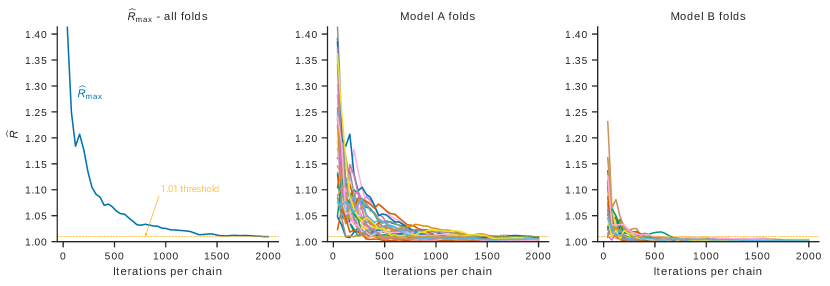
Figure 9: Progressive $\widehat{\mathrm{R}}$ statistics for folds of Example 2 (rat weight). At least one fold $\widehat{\mathrm{R}}$ value (and hence $\widehat{R}_{\mathrm{max}}$) remains above the 1.01 threshold for at least 1,750 iterations per chain, well beyond the point where the results have stabilized.

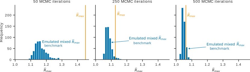
Figure 10: $\widehat{R}_{\mathrm{max}}$ and simulated mixed threshold for three different sample sizes in Example 2 (rat weight). The plots suggest the chains have not mixed after 50 iterations, but are well mixed after 500 iterations.

		Problem size			Samples / chain			Wall time (s)
		chains	posteriors		warmup	sampling		warmup*		sampling
Full-data ($M_{A}$)		8	1		7,000	2,000		14.	7	0.	5
Full-data ($M_{B}$)		8	1		7,000	2,000		10.	5	0.	5
PCV ($M_{A}$ vs $M_{B}$)		480	60		1,000	500		10.	0	7.	9

Table 2: Summary of parallel leave-case-out CV for Example 2 (rat weight). Inference was performed on a 2.0 GHz Intel Xeon Cascade Lake-SP CPU with a NVIDA T4 GPU provided by Google Colab. * Includes JAX compilation time.

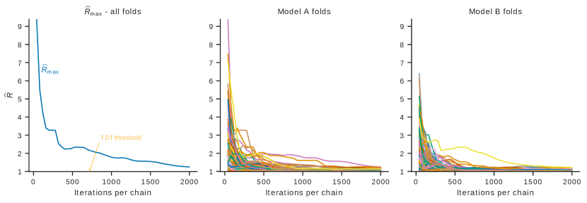
Figure 11: Progressive $\widehat{\mathrm{R}}$ statistics for folds of Example 3 (home radon). $\widehat{R}_{\mathrm{max}}$ remains above $1.01$ for all 4,000 iterations.

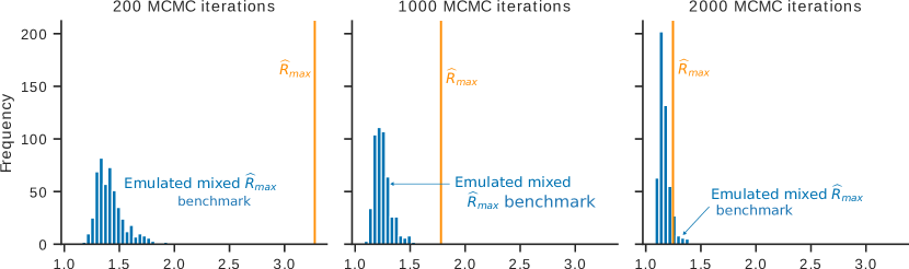
Figure 12: $\widehat{R}_{\mathrm{max}}$ for three different sample sizes in Example 3 (home radon), under log loss. The benchmark is computed with 5 breaks and 500 draws. The plots suggest the results have converged by 4,000 iterations. However, notice that the $\widehat{R}_{\mathrm{max}}$ value is well above the $1.01$ threshold suggested by Vehtari et al [48].

		Problem size			Samples / chain			Wall time (s)
		chains	posteriors		warmup	sampling		warmup*		sampling
Full-data ($M_{A}$)		4	1		7,000	5,000		36.	8	9.	4
Full-data ($M_{B}$)		4	1		7,000	5,000		28.	8	7.	9
PCV ($M_{A}$ vs $M_{B}$)		3,088	772		2,000	2,000		47.	1	45.	2

Table 3: Summary of parallel CV for Example 3 (home radon). Inference was performed on a 2.0 GHz Intel Xeon Cascade Lake-SP CPU with a NVIDA A100 GPU provided by Google Colab. * Warmup includes JAX compilation.

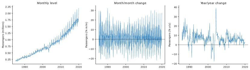
Figure 13: International air departures from all Australian airports, 1985-2019. Source: Australian Bureau of Transport and Infrastructure Research Economic (BITRE)

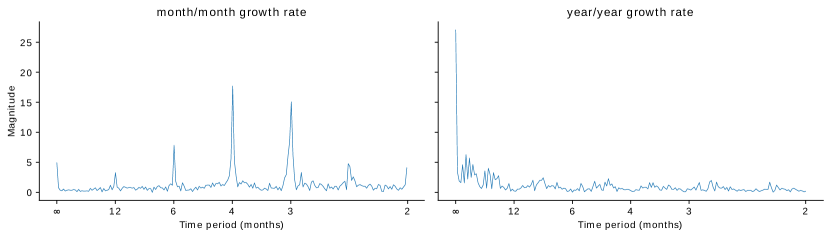
Figure 14: Power spectrum of month/month and year/year growth rates for international air departures from all Australian airports, 1985-2019. Source: Australian Bureau of Transport and Infrastructure Research Economic (BITRE) and author’s calculations.

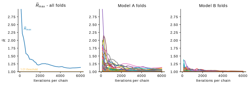
Figure 15: Progressive $\widehat{\mathrm{R}}$ statistics for folds of Example 4 (air passengers). $\widehat{R}_{\mathrm{max}}$ remains well above the 1.01 threshold for all 2,000 iterations.

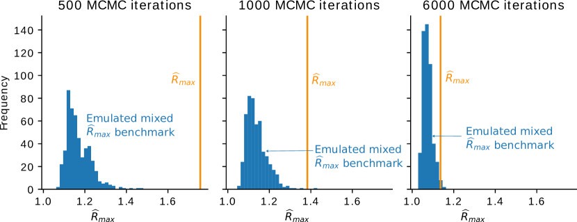
Figure 16: $\widehat{\mathrm{R}}_{\widehat{\eta}}$ for three different sample sizes in Example 4 (air passengers). The plots suggest the results have converged at 2,000 iterations.

		Problem size			Samples / chain			Wall time (s)
		chains	posteriors		warmup	sampling		warmup*		sampling
Full-data ($M_{A}$)		4	1		10,000	2,000		19.	3	2.	5
Full-data ($M_{B}$)		4	1		10,000	2,000		15.	4	2.	0
PCV ($M_{A}$ vs $M_{B}$)		3,160	790		6,000	6,000		12.	9	9.	8

Table 4: Summary of parallel CV for Example 4 (air passengers). Inference was performed on a 2.0 GHz Intel Xeon Skylake CPU with a NVIDA T4 GPU provided by Google Colab. *Warmup includes JAX JIT compilation step.

Appendix D Example code

This section presents minimal implementations of parallel CV sampler for $\mathrm{LogS}$ using python 3.10 and the JAX and BlackJAX libraries. For simplicity, the code presented here assesses predictive ability from a single model (it does not perform model selection). For a complete examples, please see https://github.com/kuperov/ParallelCV.

D.1 Non-online parallel sampler

import jax
import jax.numpy as jnp

def pcv_LogS_sampler(key, log_dens_fn, log_pred_fn, init_pos, K, L, N, kparam):
    """Non-online sampler for parallel cross-validation using LogS for a single model.

    Generates the predictive draws required to compute the elpd. Invoke this function
    twice to implement Algorithm 1 (once for warmup, once for sampling).

    Args:
        key: JAX PRNG key array
        log_dens_fn: log density function with signature (params, fold_id)
        log_pred_fn: log predictive density function with signature (params, fold_id)
        init_pos: K*L*p pytree of initial positions for each fold and chain
        K: number of folds
        L: number of chains
        N: chain length
        kparam: dictionary of hyperparameters for Blackjax HMC kernel

    Returns:
        Tuple: (lpred_draws, E)
    """
    def run_chain(init_pos, chain_key, fold_id, C):  # sample from a single chain
        fold_log_dens_fn = lambda params: log_dens_fn(params, fold_id)
        hmc_kernel = bj.hmc(fold_log_dens_fn, **kparam)

        def mcmc_step(carry_state, _): # a single mcmc step
            key, prev_state, E = carry_state
            step_key, carry_key = jax.random.split(key)
            state, info = hmc_kernel.step(step_key, prev_state)  # one mcmc step
            lpred_draw = log_pred_fn(state.position, fold_id)  # cond. log predictive
            E = E + info.is_divergent
            return (carry_key, state, E), lpred_draw

        init_state = hmc_kernel.init(init_pos)
        return jax.lax.scan(mcmc_step, (chain_key, init_state, 0), None, length=N)

    def run_fold(fold_key, ch_init_pos, fold_id, C): # run L chains for one fold
        sampling_fn = jax.vmap(lambda pos, key: run_chain(pos, key, fold_id, C))
        return sampling_fn(ch_init_pos, jax.random.split(fold_key, L))

    (_, _, E), lpred_draws = \
        jax.vmap(run_fold)(jax.random.split(key, K), init_pos, jnp.arange(K))
    return (lpred_draws, E)

D.2 Online parallel sampler

The function pcv_LogS_sampler samples from $K\times L$ posteriors in parallel and computes the statistics $V_{x}$, $V_{x^{2}}$, $U_{x}$, $U_{x^{2}}$, $Y_{x}$, $Y_{x^{2}}$, which are required to compute $\hat{\eta}$, $\widehat{ESS}$, and $\widehat{R}_{\mathrm{max}}$ (Algorithm A2). The divergence count $E$ requires no further computation.

def pcv_LogS_sampler(key, log_dens_fn, log_pred_fn, init_pos, C_k, L, H, G, D, kparam):
    """Sampler for parallel cross-validation using LogS for a single model.

    Generates the statistics required to estimate ESS, MCSE, Rhat_max, and
    the Rhat_max benchmark. Space complexity is O(K*L*D), independent of
    G and H and therefore constant with respect to MCMC chain length.

    Args:
        key: JAX PRNG key array
        log_dens_fn: log density function with signature (params, fold_id)
        log_pred_fn: log predictive density function with signature (params, fold_id)
        init_pos: K*L*p pytree of initial positions for each fold and chain
        C_k: K-array of centering constants per fold
        L: number of chains
        H: MCMC draws per batch
        G: number of batches per block
        D: number of shuffle blocks
        kparam: dictionary of hyperparameters for Blackjax HMC kernel

    Returns:
        Tuple: (last_state, Ux, Ux2, Vx, Vx2, Yx, Yx2, E)
    """
    K = C_k.shape[0]

    def run_chain(init_pos, chain_key, fold_id, C):  # sample from a single chain
        fold_log_dens_fn = lambda params: log_dens_fn(params, fold_id)
        hmc_kernel = bj.hmc(fold_log_dens_fn, **kparam)

        def mcmc_step(carry_state, _): # a single mcmc step
            key, prev_state, Zx, Ux2, Yx, Yx2, E = carry_state
            step_key, carry_key = jax.random.split(key)
            params, info = hmc_kernel.step(step_key, prev_state)  # one mcmc step
            lpred = log_pred_fn(params.position, fold_id)  # cond. log predictive
            E = E + info.is_divergent
            Zx = jnp.logaddexp(Zx, lpred)  # increment accumulators
            Ux2 = jnp.logaddexp(Ux2, 2*lpred)
            Yx += lpred - C
            Yx2 += (lpred - C)**2
            return (carry_key, params, Zx, Ux2, Yx, Yx2, E), None

        def batch_step(batch_carry, _): # one batch of H mcmc steps
            key, init_state, Vx, Vx2, Ux, Ux2, Yx, Yx2, E = batch_carry
            init_carry = (key, init_state, -jnp.inf, Ux2)
            (carry_key, state, Zx, Ux2), _ = \
                jax.lax.scan(mcmc_step, init_carry, None, length=H)
            Zx_bar = Zx - jnp.log(H)  # this batch mean
            Vx = jnp.logaddexp(Vx, Zx_bar)  # increment accumulators
            Vx2 = jnp.logaddexp(Vx2, 2*Zx_bar)
            Ux = jnp.logaddexp(Ux, Zx)
            return (carry_key, state, Vx, Vx2, Ux, Ux2, Yx, Yx2, E), None

        def block_step(block_carry, _): # one block of G batches
            init_carry = block_carry + (0, 0,)
            (key, prev_state, Ux, Ux2, Vx, Vx2, Yx, Yx2, E), _ = \
                jax.lax.scan(batch_step, init_carry, None, length=G)
            return (key, prev_state, Ux, Ux2, Vx, Vx2, E), (Yx, Yx2)

        init_state = hmc_kernel.init(init_pos)
        init_carry = (chain_key, init_state, -jnp.inf, -jnp.inf, -jnp.inf, -jnp.inf)
        return jax.lax.scan(block_step, init_carry, None, length=D)

    def run_fold(fold_key, ch_init_pos, fold_id, C): # run L chains for one fold
        sampling_fn = jax.vmap(lambda pos, key: run_chain(pos, key, fold_id, C))
        return sampling_fn(ch_init_pos, jax.random.split(fold_key, L), fold_id)

    (_, last_state, Vx, Vx2, Ux, Ux2, E), (Yx, Yx2) = \
        jax.vmap(run_fold)(jax.random.split(key, K), init_pos, jnp.arange(K), C_k)
    return (last_state, Ux, Ux2, Vx, Vx2, Yx, Yx2, E)

References

- \bibcommenthead
- Chen et al [2014] Chen T, Fox E, Guestrin C (2014) Stochastic gradient Hamiltonian Monte Carlo. In: International conference on machine learning, PMLR, pp 1683–1691
- Cooper et al [2023] Cooper A, Simpson D, Kennedy L, et al (2023) Cross-validatory model selection for Bayesian autoregressions with exogenous regressors. Preprint at http://arxiv.org/abs/2301.08276, 2301.08276
- Cowles et al [1999] Cowles MK, Roberts GO, Rosenthal JS (1999) Possible biases induced by MCMC convergence diagnostics. Journal of Statistical Computation and Simulation 64(1):87–104. 10.1080/00949659908811968
- Dawid and Musio [2014] Dawid AP, Musio M (2014) Theory and applications of proper scoring rules. METRON 72(2):169–183. 10.1007/s40300-014-0039-y
- Dawid and Musio [2015] Dawid AP, Musio M (2015) Bayesian model selection based on proper scoring rules. Bayesian Analysis 10(2):479–499. 10.1214/15-BA942
- Dawid and Sebastiani [1999] Dawid AP, Sebastiani P (1999) Coherent dispersion criteria for optimal experimental design. The Annals of Statistics 27(1):65–81
- Dillon et al [2017] Dillon JV, Langmore I, Tran D, et al (2017) TensorFlow distributions. arXiv preprint arXiv:171110604
- Gagnon et al [2023] Gagnon P, Maire F, Zanella G (2023) Improving multiple-try metropolis with local balancing. Journal of Machine Learning Research 24(248):1–59. URL http://jmlr.org/papers/v24/22-1351.html
- Geisser [1975] Geisser S (1975) The predictive sample reuse method with applications. Journal of the American Statistical Association 70(350):320–328. 10.1080/01621459.1975.10479865
- Gelfand et al [1990] Gelfand AE, Hills SE, Racine-Poon A, et al (1990) Illustration of Bayesian inference in normal data models using Gibbs sampling. Journal of the American Statistical Association 85(412):972–985
- Gelfand et al [1992] Gelfand AE, Dey DK, Chang H (1992) Model determination using predictive distributions, with implementation via sampling-based methods (with discussion). Bayesian Statistics 4
- Gelman and Hill [2006] Gelman A, Hill J (2006) Data analysis using regression and multilevel/hierarchical models. Cambridge university press
- Gelman and Rubin [1992] Gelman A, Rubin DB (1992) Inference from iterative simulation using multiple sequences. Statistical Science 7(4):457–472. URL http://www.jstor.org/stable/2246093
- Gelman et al [2014] Gelman A, Carlin JB, Stern HS, et al (2014) Bayesian data analysis, 3rd edn. Chapman & Hall/CRC, Boca Raton, FL, USA
- Gelman et al [2020] Gelman A, Vehtari A, Simpson D, et al (2020) Bayesian workflow. Preprint at http://arxiv.org/abs/2011.01808, 2011.01808
- Geyer [1992] Geyer CJ (1992) Practical markov chain monte carlo. Statistical science pp 473–483
- Glatt-Holtz et al [2022] Glatt-Holtz NE, Holbrook AJ, Krometis JA, et al (2022) Parallel MCMC algorithms: Theoretical foundations, algorithm design, case studies. arXiv preprint arXiv:220904750
- Gneiting and Raftery [2007] Gneiting T, Raftery AE (2007) Strictly proper scoring rules, prediction, and estimation. Journal of the American Statistical Association 102(477):359–378. 10.1198/016214506000001437
- Hoffman and Sountsov [2022] Hoffman MD, Sountsov P (2022) Tuning-Free Generalized Hamiltonian Monte Carlo
- Hoffman et al [2014] Hoffman MD, Gelman A, et al (2014) The No-U-Turn sampler: adaptively setting path lengths in Hamiltonian Monte Carlo. J Mach Learn Res 15(1):1593–1623
- Holbrook [2023] Holbrook AJ (2023) A quantum parallel Markov chain Monte Carlo. Journal of Computational and Graphical Statistics pp 1–14
- Holbrook et al [2021] Holbrook AJ, Lemey P, Baele G, et al (2021) Massive parallelization boosts big bayesian multidimensional scaling. Journal of Computational and Graphical Statistics 30(1):11–24. 10.1080/10618600.2020.1754226, URL https://doi.org/10.1080/10618600.2020.1754226, pMID: 34168419, https://doi.org/10.1080/10618600.2020.1754226
- Hyvärinen and Dayan [2005] Hyvärinen A, Dayan P (2005) Estimation of non-normalized statistical models by score matching. Journal of Machine Learning Research 6(4)
- Jones et al [2006] Jones GL, Haran M, Caffo BS, et al (2006) Fixed-width output analysis for Markov chain Monte Carlo. Journal of the American Statistical Association 101(476):1537–1547. 10.1198/016214506000000492
- Krüger et al [2021] Krüger F, Lerch S, Thorarinsdottir T, et al (2021) Predictive inference based on Markov chain Monte Carlo output. International Statistical Review 89(2):274–301. 10.1111/insr.12405
- Kumar et al [2019] Kumar R, Carroll C, Hartikainen A, et al (2019) ArviZ: a unified library for exploratory analysis of bayesian models in python. Journal of Open Source Software
- Lao and Louf [2020] Lao J, Louf R (2020) Blackjax: A sampling library for JAX. http://github.com/blackjax-devs/blackjax
- Lao et al [2020] Lao J, Suter C, Langmore I, et al (2020) tfp.mcmc: Modern Markov Chain Monte Carlo Tools Built for Modern Hardware. URL http://arxiv.org/abs/2002.01184, 2002.01184
- Magnusson et al [2020] Magnusson M, Vehtari A, Jonasson J, et al (2020) Leave-one-out cross-validation for Bayesian model comparison in large data. In: Chiappa S, Calandra R (eds) Proceedings of the Twenty Third International Conference on Artificial Intelligence and Statistics, Proceedings of Machine Learning Research, vol 108. PMLR, pp 341–351, URL https://proceedings.mlr.press/v108/magnusson20a.html
- Mahoney et al [2023] Mahoney MJ, Johnson LK, Silge J, et al (2023) Assessing the performance of spatial cross-validation approaches for models of spatially structured data. Preprint at https://arxiv.org/abs/2303.07334
- Margossian et al [2023] Margossian CC, Hoffman MD, Sountsov P, et al (2023) Nested : Assessing the convergence of Markov chain Monte Carlo when running many short chains. Preprint at http://arxiv.org/abs/2110.13017, 2110.13017
- Moins et al [2023] Moins T, Arbel J, Dutfoy A, et al (2023) On the use of a local to improve mcmc convergence diagnostic. Bayesian Analysis TBA(TBA):TBA
- Neal [2011] Neal RM (2011) MCMC using Hamiltonian dynamics. In: Handbook of Markov Chain Monte Carlo, vol 2. CRC Press New York, NY, p 113–162
- Neiswanger et al [2014] Neiswanger W, Wang C, Xing EP (2014) Asymptotically exact, embarrassingly parallel MCMC. In: Proceedings of the Thirtieth Conference on Uncertainty in Artificial Intelligence. AUAI Press, Arlington, Virginia, USA, UAI’14, p 623–632
- Nissen [2023] Nissen JN (2023) What scientists must know about hardware to write fast code. https://viralinstruction.com/posts/hardware/, accessed: 2023-01-09
- Racine [2000] Racine J (2000) Consistent cross-validatory model-selection for dependent data: hv-block cross-validation. Journal of Econometrics 99(1):39–61. https://doi.org/10.1016/S0304-4076(00)00030-0
- Robert and Casella [2004] Robert CP, Casella G (2004) Monte Carlo statistical methods. Springer Location New York, NY
- Roberts et al [2017] Roberts DR, Bahn V, Ciuti S, et al (2017) Cross-validation strategies for data with temporal, spatial, hierarchical, or phylogenetic structure. Ecography 40(8):913–929
- Roy [2020] Roy V (2020) Convergence diagnostics for Markov chain Monte Carlo. Annual Review of Statistics and Its Application 7:387–412
- Rubin [1981] Rubin DB (1981) The Bayesian Bootstrap. The Annals of Statistics 9(1):130 – 134. 10.1214/aos/1176345338
- Scott et al [2016] Scott S, Blocker A, Bonassi F, et al (2016) Bayes and big data: The consensus Monte Carlo algorithm. International Journal of Management Science and Engineering Management 11(2):78–88. 10.1080/17509653.2016.1142191
- Shao et al [2019] Shao S, Jacob PE, Ding J, et al (2019) Bayesian model comparison with the hyvärinen score: Computation and consistency. Journal of the American Statistical Association
- Sivula et al [2022] Sivula T, Magnusson M, Matamoros AA, et al (2022) Uncertainty in Bayesian leave-one-out cross-validation based model comparison. Preprint at http://arxiv.org/abs/2008.10296, 2008.10296
- Stallings [2015] Stallings W (2015) Computer Organization and Architecture. Pearson Education, Limited
- Stan Development Team [2022] Stan Development Team (2022) Stan Modeling Language: User’s Guide and Reference Manual
- Vehtari and Lampinen [2002] Vehtari A, Lampinen J (2002) Bayesian model assessment and comparison using cross-validation predictive densities. Neural Computation 14(10):2439–2468. 10.1162/08997660260293292
- Vehtari et al [2017] Vehtari A, Gelman A, Gabry J (2017) Practical Bayesian model evaluation using leave-one-out cross-validation and WAIC. Statistical Computing 27(5):1413–1432. 10.1007/s11222-016-9696-4
- Vehtari et al [2020a] Vehtari A, Gelman A, Simpson D, et al (2020a) Rank-normalization, folding, and localization: An improved for assessing convergence of MCMC. Bayesian Analysis -1(-1):1–26. 10.1214/20-ba1221
- Vehtari et al [2020b] Vehtari A, Gelman A, Sivula T, et al (2020b) Expectation propagation as a way of life: A framework for bayesian inference on partitioned data. Journal of Machine Learning Research 21(17):1–53. URL http://jmlr.org/papers/v21/18-817.html
- Warne et al [2022] Warne DJ, Sisson SA, Drovandi C (2022) Vector operations for accelerating expensive bayesian computations–a tutorial guide. Bayesian Analysis 17(2):593–622
- Welford [1962] Welford BP (1962) Note on a method for calculating corrected sums of squares and products. Technometrics 4(3):419–420