Cross-validatory model selection for Bayesian autoregressions with exogenous regressors

Abstract

Bayesian cross-validation (CV) is a popular method for predictive model assessment that is simple to implement and broadly applicable. A wide range of CV schemes is available for time series applications, including generic leave-one-out (LOO) and K-fold methods, as well as specialized approaches intended to deal with serial dependence such as leave-future-out (LFO), $h$-block, and $hv$-block.

Existing large-sample results show that both specialized and generic methods are applicable to models of serially-dependent data. However, large sample consistency results overlook the impact of sampling variability on accuracy in finite samples. Moreover, the accuracy of a CV scheme depends on many aspects of the procedure. We show that poor design choices can lead to elevated rates of adverse selection.

In this paper, we consider the problem of identifying the regression component of an important class of models of data with serial dependence, autoregressions of order $p$ with $q$ exogenous regressors ($\operatorname{\mathsf{ARX}\!}(p,q)$), under the logarithmic scoring rule. We show that when serial dependence is present, scores computed using the joint (multivariate) density have lower variance and better model selection accuracy than the popular pointwise estimator. In addition, we present a detailed case study of the special case of $\operatorname{\mathsf{ARX}\!}$ models with fixed autoregressive structure and variance. For this class, we derive the finite-sample distribution of the CV estimators and the model selection statistic. We conclude with recommendations for practitioners.

2301.08276

,

1 Overview

Many workflows for constructing predictive Bayesian models require the practitioner to choose the best model among a number of candidates according to their predictive power for the task at hand. Although many predictive model selection methods are available (Vehtari and Ojanen, 2012), among the most popular is cross-validation (CV; Geisser, 1975). CV is flexible and applicable to a wide variety of statistical applications.

In finite samples, CV-based selection objectives are biased and subject to sampling variation, which leads to uncertainty about model predictive ability and the possibility of adverse model selection (Arlot and Celisse, 2010; Sivula et al., 2020). In the Bayesian context, there is a large literature on the frequency properties (i.e. variability across multiple realizations of a dataset) of model selection rules using information criteria such as the widely-available information criterion (WAIC) and the Bayes factor (e.g., Ward, 2008; Schad et al., 2022). Despite its popularity in Bayesian applications, however, less is known about the frequency properties of dependent CV procedures for Bayesian model selection under log-predictive loss.

Recent work by Sivula et al. (2020) analyzed the frequency properties of leave-one-out CV (LOO-CV) for Bayesian regression models of exchangeable data. The authors identify at least three scenarios that lead to elevated uncertainty in CV model selection, and therefore to an increased probability of adverse model choice. These pathological cases include comparisons between candidate models that produce similar predictions, where models are badly misspecified, and where training data sizes are small.

In this study, we extend the analysis of Sivula et al. (2020) to Bayesian models of serially dependent data. We aim to characterize CV model selection uncertainty for a simple but important class of models: autoregressions of order $p$ with $q$ exogenous regressors, $\operatorname{\mathsf{ARX}\!}(p,q)$. Our goal is to identify the regression component of the model under the logarithmic scoring rule, leaving to one side the related task of identifying the autoregressive component. In this context, a scoring rule is a loss function for assessing the quality of probabilistic predictions (Gneiting and Raftery, 2007). While many scoring rules are available, we focus on the logarithmic scoring rule, for which a measure of predictive performance is the expected log predictive density (elpd) described in Section 2.2.

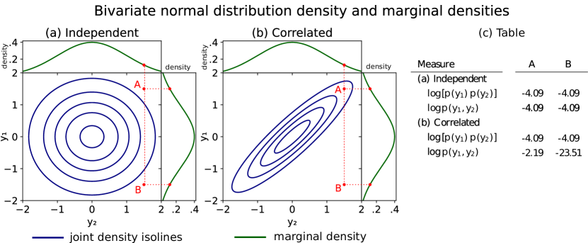
Figure 1: Illustration of the distinction between joint and pointwise log density measures in correlated models. Both plots show bivariate normal densities centered at the origin with unit marginal variance and correlation coefficients of 0 (Panel (a)) and 0.9 (Panel (b)). Panel (c) tabulates joint and pointwise log densities evaluated at the marked points A and B, indicated in red on the plots. In the correlated case, only the joint log density, $\log p\left(y_{1},y_{2}\right)$, identifies point B as having low log density. In contrast, the pointwise density $\log p\left(y_{1},y_{2}\right)$ is the same for both.

We address two important aspects of scoring rule design for models of correlated data. First, whether the scoring rule used for model assessment will be univariate or multivariate. Second, for multivariate scoring rules, whether it will be evaluated jointly (as a multivariate predictive density) or pointwise (as univariate marginal densities). We begin with a demonstration of the importance of the latter, showing improved statistical power of model selection with a jointly-evaluated scoring rule. We continue with a detailed case study of model selection under several popular CV schemes. This comparison includes several specific univariate (pointwise) methods, and several joint methods. Throughout, we find that joint methods achieve greater (statistical) efficiency, measured as lower adverse selection rates, and the associated CV estimators tend to have have lower variability.

Figure 1 illustrates the importance of joint multivariate assessments when data are correlated. The figure shows two bivariate normal distributions. In one the variates are mutually independent, and in the other they are strongly correlated. The table shows that points A and B have identical pointwise log densities under both distributions, even though point B lies in a region of very low (joint) density in the correlated case. We conclude that in contrast to the joint approach, when correlation is strong the pointwise density fails to detect that point B is in a region of low probability for this model.

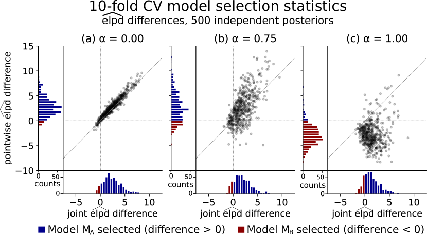
Figure 2: Joint log-score differences versus pointwise log score differences, computed using 10-fold-CV in a model selection statistics for 500 independent posteriors of the ‘hard’ case (see Section 3). The DGP is a stationary $\operatorname{\mathsf{ARX}\!}\left(2,3\right)$ and candidate models are $M_{A}:\,\operatorname{\mathsf{ARX}\!}\left(1,2\right)$ and $M_{B}:\,\operatorname{\mathsf{ARX}\!}\left(1,1\right)$. Model selection statistics are expected log pointwise predictive density ($\operatorname{elpd}$) differences. The DGP has autoregressive parameter $\phi_{*}=\alpha\left(0.75,0.2\right)$ so that $\alpha$ selects increasing serial dependence from left to right. Adverse selection increases for the pointwise method (vertical axis) as dependence increases. See Section 3 for a full description.

To further motivate our approach, Figure 2 previews the results of a model selection experiment we will describe in more detail in Section 3. The figure compares the distribution of CV model selection statistics for selecting between two candidate $\operatorname{\mathsf{ARX}\!}$ models. The panels show increasing degrees of dependence from left to right. As dependence increases, the pointwise model selection statistic shows an increasing rate of adverse model selection (red bars in the vertical margin). In contrast, there is little change for the jointly-evaluated case (red bars in the horizontal margin). For a full description of this experiment, please refer to Section 3.

Several CV strategies are available for models of serially dependent data, and there seems to be little agreement in the literature about which one practitioners should adopt, especially in the Bayesian modeling literature. Furthermore, much of the existing literature addresses different blocking strategies, but does not make a distinction between joint and pointwise evaluation of the scoring rule. Moreover, we speculate that different CV schemes will be useful when assessing different aspects of such a model. Even when the analytical focus is not the autoregressive component, joint predictive measures appear to be useful for identifying the regression components.

In contrast to much of the existing literature on CV for autoregressive models, including many large-sample consistency results (e.g., Bergmeir et al., 2018; Racine, 2000), our emphasis is on the frequency properties of the CV estimator in finite samples. Further to the three problematic scenarios identified by Sivula et al. (2020), our results suggest that strong serial dependence and a cross-validatory objective function that does not capture model dynamics (e.g. pointwise objectives) can pose difficulties for CV-based model selection, even when the goal is not limited to identification of the autoregressive component of the model. Our results stand as a counterpoint to large-sample consistency results and suggest that mere consistency of the estimator is not enough. That is, under certain choices of the CV scheme the variance of the model selection statistic can be very high, leading to elevated rates of adverse selection.

1.1 Contributions

We present novel results for procedures that use CV methods under the logarithmic scoring function when serial dependence is present. Working with the logarithmic scoring function and focusing on identifying the regression component of the model, we demonstrate that:

• Under serial dependence, CV schemes should be designed to account for the presumed dependence structure of the data in order to achieve good model selection performance;

• When serial dependence is strong, performance measures evaluated jointly are much more (statistically) efficient than pointwise counterparts;

• When the sample size is finite, there is a U-shaped relationship between certain CV scheme hyperparameters and the adverse selection rate;

• We present novel results on the variability of Bayesian CV procedures for $\operatorname{\mathsf{ARX}\!}(p,q)$ models. To our knowledge, these are among the first results describing the finite-sample uncertainty of CV methods under serial dependence, particularly in a Bayesian setting.

We offer the following advice for practitioners working with models of serially-dependent data. Broadly speaking, since CV methods based on joint scoring rules are usually more complex to implement, their improved efficiency should be traded off against implementation burden. Following model criticism of each candidate model ahead of model selection, we recommend:

• Where measured serial dependence in the data is not very strong, simpler pointwise CV methods (like LOO-CV and LFO-CV) can be used as a first-pass, and relied upon where the results are clear (see Sivula et al., 2020, for criteria);

• Otherwise, if serial dependence is strong or results are unclear then joint CV model selection methods should be implemented instead.

• Even when the actual predictive task requires a univariate prediction (like a one-step-ahead prediction), for model selection it may be better to use a CV scheme that leaves out multiple observations, combined with a multivariate scoring rule.

The remainder of the paper proceeds as follows. In Section 2 we describe the model class and summarize CV-based model selection and some relevant literature, highlighting some key challenges associated with CV for dependent data. Section 3 presents a short simulation experiment, and Section 4 presents a detailed case study of CV model selection in a simplified form of $\operatorname{\mathsf{ARX}\!}$ model, focusing on the properties of CV under dependence and demonstrating where challenges can arise. Finally, Section 5 discusses the results and concludes. See https://github.com/kuperov/arx for code and experiments.

2 Background

In this section, we briefly review CV model selection and review some relevant literature. We will suppose we have observed a data vector $y=\left(y_{1},\dots,y_{T}\right)$, presumed to be drawn from a joint distribution $p_{\mathrm{true}}$, the (typically unknown) data-generating process (DGP). Our goal is to construct predictions by first selecting the best available model $M^{*}$ from some set $\mathcal{M}$ of candidates (or candidate model families identified up to a parameter). This selection is made according to candidate models’ ability to predict as-yet unseen realizations of the process, that is, by their out-of-sample predictive power.

To simplify our analysis, we will consider only pairwise comparisons (i.e. $\left|\mathcal{M}\right|=2$), but we do explicitly allow that $M_{\mathrm{true}}\not\in\mathcal{M}$, i.e. the model associated with $p_{\mathrm{true}}$ is not in $\mathcal{M}$.

2.1 Autoregressions with exogenous regressors

We will write $\operatorname{\mathsf{ARX}\!}\left(p,q\right)$ for an autoregression with $p$ lags of the dependent variable and $q$ exogenous regressors. Throughout we assume $p\ll T$ and $q\ll T$, and that $T$ is ‘small’, corresponding to common applied settings where data are limited.

The $\operatorname{\mathsf{ARX}\!}\left(p,q\right)$ class is a key building block for time series models in a wide range of scientific, policy, and business applications. For instance, autoregressions underpin the popular vector autoregression (VAR) models used by macroeconomic policymakers (e.g., Sims, 1980) and spatial epidemiological studies (Lee, 2011).

The $\operatorname{\mathsf{ARX}\!}\left(p,q\right)$ model is conditionally normal,

$$p\left(y_{t}|\phi,\beta,y_{t-1},\dots,y_{t-p}\right) =\mathcal{N}\left(y_{t}|\phi_{1}y_{t-1}+\cdots+\phi_{p}y_{t-p}+z_{t}^{\top}\beta,\sigma^{2}\right),$$ (2.1)

for $t=1,\dots,T$, where the first element of the $q\times 1$ vector of exogenous variables $z_{t}$ is $1$. For simplicity, we will initialize the sequence from zero, so that $y_{1-p}=\cdots=y_{0}=0$.

In comparison to the linear regression (LR) model studied by Sivula et al. (2020), the dependence structure of the $\operatorname{\mathsf{ARX}\!}$ class substantially complicates the analysis. Naturally, one could view the lags of $y_{t}$ as explanatory variables which would mean the $\operatorname{\mathsf{ARX}\!}\left(p,q\right)$ model is identical to that of the Gaussian linear regression (LR) analyzed by Sivula et al. (2020). However, to restrict our attention to models in the stationary regime, we must either impose informative priors on the autoregressive parameters (as we do in Section 3) or fix them (as we do in Section 4). In both Sections 3 and 4 we we have allowed analytical convenience to guide the choice of prior.

It is worth emphasizing that all the results we present in this paper depend on $Z$, the $T\times q$ matrix of exogenous covariates. Our results do not need to make any assumptions about the distribution of $Z$, since they are assumed known and fixed. In our experiments, we construct $Z$ by drawing a matrix of independent standard normal variates, a matrix we keep fixed across all replicates of each experiment.

2.2 Predictive model selection

When the goal of a modeling exercise is prediction, it is natural to use predictive performance as a measure of model goodness or ‘utility’. Predictive performance can be assessed using a scoring rule, a function that produces a numerical assessment of a probabilistic prediction against actual observations (Gneiting and Raftery, 2007). Since the choice of scoring rule governs the selection of $M^{*}$, an ideal choice for a scoring rule would be tailored to the modeling task at hand. However, in the absence of a specific application, general-purpose scoring rules are available.

We focus on the popular logarithmic scoring rule, which enjoys the mathematical properties of being local and strictly proper and is closely related to the KL divergence (Gneiting and Raftery, 2007; Vehtari and Ojanen, 2012; Dawid, 1984). Under the logarithmic score, we call the expected score for some model $M_{\ell}$ the expected log joint predictive density (eljpd),

$$\operatorname{eljpd}\left(M_{\ell}|y\right) =\mathbb{E}_{\tilde{y}\sim p_{\mathrm{true}}}\left[\log\int p\left(\tilde{y}|\theta,M_{\ell}\right)p\left(\theta\,|\,y,M_{\ell}\right)\,\mathrm{d}\theta\right]$$ (2.2)

$$=\mathbb{E}_{\tilde{y}\sim p_{\mathrm{true}}}\left[\log p\left(\tilde{y}|y,M_{\ell}\right)\right]$$ (2.3)

where ‘joint’ refers to the fact that the multivariate predictive $p\left(\tilde{y}|y,M_{\ell}\right)$ is a joint density. Here, the $T\times 1$ random variable $\tilde{y}$ is independent of the data $y$.

If $p_{\mathrm{true}}$ were known or unlimited independent replicates $\tilde{y}\sim p_{\mathrm{true}}$ were available so that (2.2) could be evaluated, the utility-maximizing model $M^{*}$ could be selected by ‘external validation’ (Gelman et al., 2014) of the model $M_{\ell}$ joint predictive $p\left(\cdot|y,M_{\ell}\right)$ with respect to $p_{\mathrm{true}}$,

$$M^{*}:=\arg\max_{M_{\ell}\in\mathcal{M}}\operatorname{eljpd}\left(M_{\ell}|y\right)=\arg\max_{M_{\ell}\in\mathcal{M}}\mathbb{E}_{\tilde{y}\sim p_{\mathrm{true}}}\left[\log p\left(\tilde{y}|y,M_{\ell}\right)\right].$$ (2.4)

In many cases it is computationally convenient to compute (2.3) in a pointwise fashion, which yields the expected log pointwise predictive density (elppd),

$$\operatorname{elppd}\left(M_{\ell}|y\right) =\mathbb{E}_{\tilde{y}\sim p_{\mathrm{true}}}\left[\log\prod_{t=1}^{T}\int p\left(\tilde{y}_{t}|\theta\right)p\left(\theta\,|\,y,M_{\ell}\right)\,\mathrm{d}\theta\right]$$ (2.5)

$$=\mathbb{E}_{\tilde{y}\sim p_{\mathrm{true}}}\left[\sum_{t=1}^{T}\log p\left(\tilde{y}_{t}|y,M_{\ell}\right)\right],$$ (2.6)

The pointwise predictive $p\left(\tilde{y}_{t}\,|\,\theta,M_{\ell}\right)$ that appears in (2.6) is simply the multivariate predictive with all but one $\tilde{y}$ element marginalized out,

$$p\left(\tilde{y}_{t}|y,M_{\ell}\right)=\int\!\cdots\!\int p\left(\tilde{y}|y,M_{\ell}\right)\,\prod_{s\neq t}\mathrm{d}\tilde{y}_{s}.$$ (2.7)

The resulting utility measure for model $M_{\ell}\in\mathcal{M}$ given observed data $y$ can be computed using the model joint predictive density. We will often want to discuss both classes of expected predictive densities in a generic sense, in which case we will use the umbrella term expected log predictive density (elpd).

We adopt (2.4) as our benchmark for the preferred model. From this perspective, the pointwise density (elppd) is useful to the extent that it is a computationally convenient approximation of the joint density (eljpd). It is important to note that while elppd and eljpd are both useful for making comparisons against similarly-constructed measures, they are fundamentally different quantities. See, for instance, Madiman and Tetali (2010) for inequalities between joint and pointwise densities.

When observations are conditionally independent given global model parameters, it is often the case that the $\operatorname{elppd}$ and $\operatorname{eljpd}$ are close or even identical. However, under serial and other forms of dependence, this is rarely the case because the eljpd captures additional information about serial dependence of the observations not reflected by the pointwise measure.

Unfortunately, the expected utility maximization framework described above suffers a crucial drawback: $p_{\mathrm{true}}$ is rarely ever known in practice, and thus the elpd must be estimated purely from observed data. While one might be tempted to simply substitute $p\left(y\,|\,y,M_{\ell}\right)$ into (2.3) or (2.6), this will lead to a positively biased (over-optimistic) estimate due to model overfit (Vehtari and Ojanen, 2012; Gelman et al., 2014). Instead, we need a method for estimating elppd and eljpd using only the available data.

2.3 Cross-validation

CV is a method for estimating the elpd purely from observed data by data splitting and repeated re-fits of the model. Suppose for a moment that independent replicates of the data $\tilde{y}^{(s)}\sim p_{\mathrm{true}}$, $s=1,\dots,S$, were available, and the predictive were able to be evaluated pointwise. Then the utility (2.6) under model $M_{\ell}$ could be targeted by the following Monte Carlo estimator,

$$\widehat{\operatorname{elppd}}\left(M_{\ell}|y\right)=\frac{1}{S}\sum_{s=1}^{S}\sum_{t=1}^{T}\left[\log p\left(\tilde{y}_{t}^{(s)}|y,M_{\ell}\right)\right].$$ (2.8)

In applications where such replicates are unavailable, CV estimators exploit the fact that the data $y$ are distributed according to $p_{\textnormal{true}},$ even if $p_{\textnormal{true}}$ is itself unknown. CV proceeds by repeatedly splitting the data into disjoint testing and training data subsets, estimating the model on the training set, then constructing an estimator using pointwise predictions for the testing set. The CV estimator for $\operatorname{elppd}\left(M_{\ell}|y\right)$, which divides $y$ into $K$ test sets, can be defined as

$$\widehat{\operatorname{elppd}}_{CV}\left(M_{\ell}\,|\,y\right) =\frac{T}{K}\sum_{k=1}^{K}\frac{1}{\left|\mathsf{test}_{k}\right|}\sum_{t\in\mathsf{test}_{k}}\log p\left(y_{t}\,|\,y_{\mathsf{train}_{k}},M_{\ell}\right),$$ (2.9)

where $\mathsf{test}_{k}$ denotes the subset of $y$ to be evaluated under the predictive, $\mathsf{train}_{k}$ denotes the subset of $y$ to be used to train the data. The scaling factors normalize the measure to ‘sum scale’. The corresponding joint measure is given by

$$\widehat{\operatorname{eljpd}}_{CV}\left(M_{\ell}\,|\,y\right) =\frac{T}{K}\sum_{k=1}^{K}\frac{1}{\left|\mathsf{test}_{k}\right|}\log p\left(y_{\mathsf{test}_{k}}\,|\,y_{\mathsf{train}_{k}},M_{\ell}\right).$$ (2.10)

We stress that CV schemes with multivariate test sets, like $hv$-block and $K$-block, can be evaluated in either a joint or pointwise fashion. In comparison, univariate schemes like LOO can only be evaluated pointwise.

The CV scheme blocking design is fully described by the triple $\left(K,\left\{\mathsf{test}_{k}\right\}_{k=1}^{K},\right.$ $\left.\left\{\mathsf{train}_{k}\right\}_{k=1}^{K}\right)$. Classic LOO, for instance, has $K=T$, $\mathsf{test}_{k}=\left\{k\right\}$ and $\mathsf{train}_{k}$ includes all but the $k$th element.

Model selection using cross-validation selects the model with the greatest estimated utility—or at least the simplest model similar to the best model. For a pairwise comparison between $\mathcal{M}=\left\{M_{A},M_{B}\right\}$, the CV estimate of the utility-maximizing objective is the sign of the difference

$$\widehat{\operatorname{elppd}}_{CV}\left(M_{A},M_{B}\,|\,y\right) =\widehat{\operatorname{elppd}}_{CV}\left(M_{A}\,|\,y\right)-\widehat{\operatorname{elppd}}_{CV}\left(M_{B}\,|\,y\right).$$ (2.11)

We have omitted from this formulation of the model selection objective the bias correction term that is sometimes included to account for the fact that there are fewer elements in the training set for each CV fold than in the full-data posterior. Typically a first-order correction is used, and it is usually very small (see Gelman et al., 2014).

Under correct model specification, the summands in the CV estimator (2.9) will usually be weakly correlated. Under relatively mild regularity conditions $\widehat{\operatorname{elppd}}_{CV}$ should converge to the expected utility $\operatorname{elppd}$ as $T$ grows large (see Bergmeir et al., 2018, for an analysis of LOO-CV, for instance).

2.4 CV schemes for serial dependence

In models of cross-sectional data where all observations can be assumed conditionally independent, the data structure imposes relatively few constraints on the sequence of training and test sets used for CV.

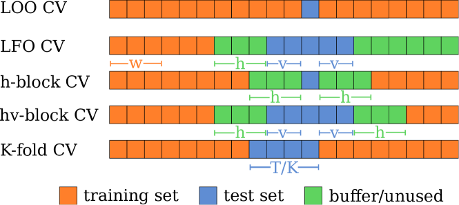
Figure 3: Cross-validation blocking schemes described in Section (2.4) for a sequence of length $T=20$. The various schemes have hyperparameters $h=3$ (h- and hv-block CV, LFO), $v=2$ (hv-block CV and LFO), $K=5$ (K-fold CV), and $w=3$ (LFO).

Under serial dependence, care is needed to ensure the contributions to (2.6) are mutually independent, or at least as independent as we can make them. To this end, a number of CV schemes have been developed specifically for models of serially dependent data.

A key consideration when selecting a CV scheme is the nature of the intended prediction task, for instance, whether the model will be used for one-step-ahead or $M$-step-ahead predictions.

Existing analyses of these schemes refer to specific contexts that do not necessarily align with our Bayesian framework. Most use different scoring functions and all but a few are analyzed with reference to classical models that yield point predictions. For our purpose, what we take from this earlier work is the design of the blocking scheme, i.e. the choices of $\left(K,\left\{\mathsf{test}_{k}\right\}_{k=1}^{K},\left\{\mathsf{train}_{k}\right\}_{k=1}^{K}\right)$. These are summarized below and illustrated in Figure 3.

Burman et al. (1994) present h-block CV, an adaptation of CV for stationary dependent sequences. In order to nearly eliminate the bias arising from dependence between train and test sets in LOO-CV, their procedure deletes a buffer of size $h$ around the training set, while retaining just a single test observation (see Figure 3). This reduces the size of the training set by $2h$ observations, but still leaves a total of $n$ test sets. They propose $h$ be a fixed proportion of the data length. Although this is ‘conservative’ (the authors refer to Györfi et al. (1989), whose results allow consistency if $h/T\longrightarrow 0$ so long as certain conditions on the underlying dependence structure are met), they argue this is appropriate because in practice the dependence structure is typically unknown. Since each $h$-block fold has a single test element, it is by definition a pointwise CV framework.

Racine (2000) proposes $hv$-block CV as an extension of $h$-block CV, which increases the test set dimension from $1$ to $2v+1$. The author claims this provides selection consistency in a wider range of circumstances, including nested models, which may be of interest in the case where model identification is the goal. Since $hv$-block has a multivariate test set, it can be evaluated jointly.

Another blocking scheme specific to serially dependent data is leave-future-out (LFO-CV; Bürkner et al., 2020). LFO-CV trains the model only on past observations, starting with a warmup period $0<w\ll T$, and leaves future observations unused. To be comparable to the other methods, our implementation of LFO mirrors the structure of $hv$-block CV (Figure 3). That is, we write $\mathrm{LFO}\left(h,v,w\right)$ for a LFO scheme that includes a halo $h\geq 0$, size parameter $v$, and initial buffer $w$. This generalized form of LFO contains the usual formulation, which is $\mathrm{LFO}(0,0,w)$.

We have also included $K$-fold CV. This method is not specific to serial dependence, although it is commonly applied under serial dependence in the literature (Cerqueira et al., 2020; Bergmeir and Benítez, 2012; Bergmeir et al., 2018). We use a variant of $K$-fold CV that partitions the sample into $K$ contiguous sub-blocks each roughly of size $T/K$. Typical values for $K$ are 5 or 10. The predictive may be evaluated jointly or pointwise, depending on the context.

3 A model selection experiment

In this section, we illustrate the behavior of CV model selection under serial dependence by repeatedly performing a model selection experiment on simulated data. We have chosen this experiment because we believe it is illustrative of general behaviors of CV for autoregressive models. We use a sequence of experiments, where we control the degree of serial dependence.

Consider the following model selection problem. Let the vector $y=y_{1},\dots,y_{T}$ be distributed according to an $\operatorname{\mathsf{ARX}\!}\left(2,3\right)$ of the following form,

$$\textnormal{DGP}:\ y_{t}=\alpha\begin{pmatrix}0.75\\ 0.2\end{pmatrix}^{\top}\begin{pmatrix}y_{t-1}\\ y_{t-2}\end{pmatrix}+\beta_{*1}+\beta_{*2}z_{2t}+\beta_{*3}z_{3t}+\sigma_{*}\varepsilon_{t},$$ (3.1)

where $\varepsilon_{t}\overset{\mathrm{iid}}{\sim}\mathcal{N}\left(0,1\right)$. The fixed parameter $\alpha\in\left[0,1\right]$ allows us to select the degree of serial dependence. When $\alpha=0$ the observations are mutually independent, and $\alpha=1$ generates a highly persistent series for the model in (3.1). All $\alpha\in[0,1]$ generate stationary series. While the upper bound $\alpha=1$ is arbitrary, corresponding to $\phi_{*}=(0.75,0.2)$, it is a useful upper limit for our experiments that generates a persistent but nonetheless stationary series. We observe similar results for other choices of the upper bound and ratio between elements of $\phi$. For simplicity, we fix initial conditions $y_{t}=0$ for $t\leq 0$.

The experiment selects between two candidate models:

$$M_{A}:\ y_{t} =\phi_{1}y_{t-1}+\beta_{1}+\beta_{2}z_{2t}+\varepsilon_{t} \operatorname{\mathsf{ARX}\!}\left(1,2\right)$$ (3.2)

$$M_{B}:\ y_{t} =\phi_{1}y_{t-1}+\beta_{1}+\varepsilon_{t} \operatorname{\mathsf{ARX}\!}\left(1,1\right).$$ (3.3)

We choose the analytically-convenient (although non-conjugate) prior,

$$\beta|\sigma^{2}\sim\mathcal{N}\left(\beta_{*},\sigma^{2}I_{p}\right),\quad\sigma^{2}\sim\mathcal{IG}\left(a_{0},b_{0}\right),\quad\phi\sim\mathcal{BE}_{(-1,1)}\left(c_{0},d_{0}\right),$$ (3.4)

where $a_{0}=b_{0}=c_{0}=d_{0}=1$. $\mathcal{IG}$ denotes the inverse-gamma density and $\mathcal{BE}_{(-1,1)}$ the beta distribution scaled to have support on $(-1,1)$.

This model is ‘fully Bayesian’ is the sense that we regard all three parameters ($\beta$, $\sigma^{2}$, and $\phi$) as unknown, and we allow them all to be estimated. For computational tractability, we have chosen conjugate priors for $\beta$ and $\sigma^{2}$, and we will conduct inference only on stationary $\operatorname{\mathsf{ARX}\!}\left(1,q\right)$ models. In this special case, $\phi$ is univariate with support on the interval $\left(-1,1\right)$. We center the $\beta$ prior on the truth $\beta_{*}$ to avoid distortions as the effective sample size changes with $\alpha$.

Both candidate models are ‘misspecified’ in the sense that neither has the same functional form as (3.1). However, while both models omit the second $y_{t}$ lag and effect $\beta_{3}$, the candidate $M_{A}$ is nonetheless the better model in the sense that it is closer in KL divergence to the DGP. This is because it includes $\beta_{2}$, which is also omitted by $M_{B}$.

We will work with two vectors of true DGP parameters $\beta_{*}$, distinguished by the relative ease with which CV is able to select the better model in our experiments:

$$\textnormal{`easy' case: }\beta_{*}^{\textnormal{easy}}=\left(1,2,1\right),\qquad\textnormal{`hard' case: }\beta_{*}^{\textnormal{hard}}=\left(1,\frac{1}{2},1\right).$$

These arbitrary parameter values were chosen for convenience in the context of our experiments and simulated covariates. $\beta_{*}^{\textnormal{easy}}$ is an example of the case where CV has little difficulty separating $M_{A}$ and $M_{B}$ under logarithmic loss, and under $\beta_{*}^{\textnormal{hard}}$ model identification by CV is much more challenging. Naturally, the relative difficulty of $\beta_{*}^{\textnormal{easy}}$ and $\beta_{*}^{\textnormal{hard}}$ depends on a range of factors, including the covariates $z_{it}$, noise variance, and data length. This setup does not make any assumptions about the distribution of the matrix $Z$ with elements $z_{it}$, other than that it is known. In our simulations, we have drawn $z_{it}\overset{\mathrm{iid}}{\sim}\mathcal{N}\left(0,1\right)$, which remain fixed throughout.

Although the posteriors associated with the above candidate models have no closed form, we are able to estimate them relatively computationally cheaply using one-dimensional quadrature or MCMC; see Appendix E for the complete computational details. The availability of efficient estimation procedures is important for our experiments because we perform CV by brute force for each simulation draw. That is, we avoid computational shortcuts like importance sampling to ensure our results are not being driven by approximation error.

Figure 2 summarizes the results of this model selection experiment. It plots model selection statistic for 500 independent simulated data sets for the ‘hard’ model variant, comparing model selection statistics from two variants of 10-fold CV. The vertical axis shows the CV objective evaluated pointwise, that is $\widehat{\operatorname{elppd}}_{\mathrm{CV}}\left(M_{A},M_{B}|y\right)$, and the horizontal axis shows the objective evaluated jointly, that is $\widehat{\operatorname{eljpd}}_{\mathrm{CV}}\left(M_{A},M_{B}|y\right)$. Adverse selection for both measures is indicated by negative selection statistics, that is those that would selection $M_{B}$. Points lying in the first quadrant, for instance, represent correct selection by both joint and pointwise methods.

Some stylized facts are evident in the Figure 2. First, when data are mutually independent (the dependence parameter $\alpha=0$, left panel) the marginal distribution and relative performance of both methods is approximately equal. However, as $\alpha\to 1$ we see that the variance of the pointwise estimates grows sharply and the location of the distribution shifts in a negative direction, indicating a sharp increase in the adverse selection rate. In contrast, the joint estimates are little changed as $\alpha$ varies. Further note that many LOO estimates fall in the fourth quadrant, indicating that the wrong model would be selected in those cases.

An equivalent experiment with the ‘easy’ parameter variant (not shown) displays a similar increase in the variability of the pointwise model selection statistic, but because the entire distribution lies far enough from the x-axis there is no appreciable increase in the adverse selection rate.

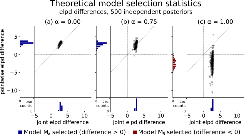
Figure 4: Joint and pointwise theoretical model selection statistics under log score for 500 independent posteriors, as dependence increases from left to right. This is the ‘hard’ example described in Section 4: the DGP is an $\operatorname{\mathsf{ARX}\!}\left(2,3\right)$ and the candidates are $M_{A}:\,\operatorname{\mathsf{ARX}\!}\left(1,2\right)$ and $M_{B}:\,\operatorname{\mathsf{ARX}\!}\left(1,1\right)$. Positive values select the $M_{A}$, the better model. The gray line is the 45 degree line where both estimators are equal. Marginal histograms are also shown, with red bars indicating adverse selection.

Figure 4 offers one explanation for the rising variance of the pointwise CV statistic. It plots the true elppd and eljpd for the 500 posteriors in Figure 2, i.e. the underlying quantities that the joint and pointwise CV estimators are targeting. The change in distributions evident in both figures is quite similar, suggesting that it is a difference between the underlying quantities, rather than some problem with the CV estimators under serial dependence, that is driving the differences between joint and pointwise 10-fold CV.

4 Detailed case study

In this section, we focus on the problem of identifying the regression component within the $\operatorname{\mathsf{ARX}\!}$ class. We will work with a simplified version of the $\operatorname{\mathsf{ARX}\!}\left(p,q\right)$, where we regard only the regression parameter $\beta$ as random, with a Gaussian prior centered on the truth, $\beta\sim\mathcal{N}\left(\beta_{*},\Sigma_{0}\right)$. This simplification allows us to focus our attention narrowly on the task of identifying $\beta$. It also makes available analytical expressions for the posterior distribution, as well as the distribution of the theoretical $\operatorname{elppd}$ and $\operatorname{eljpd}$, associated CV estimators, and model selection statistics.

This approach circumvents a key challenge associated with analyzing the variability of CV procedures: in general there are no closed-form expressions for the variance of elpd measures (Bengio and Grandvalet, 2004). However, when $\phi$ and $\sigma^{2}$ are fixed, a closed form does exist. The existence of closed form expressions allows us to derive the finite-sample distribution of the elpd for all of the CV procedures we consider.

4.1 Utility measures and model selection statistic

In this simple case, we can obtain exact distributions for the joint $\operatorname{eljpd}$ and pointwise $\operatorname{elppd}$ for the $\operatorname{\mathsf{ARX}\!}$ class with fixed $\phi_{*}$ and $\sigma_{*}^{2}$, as well as their associated CV estimators. The results in this section extend earlier results for the $\operatorname{elppd}$ and LOO-CV derived by Sivula et al. (2020), in the case of i.i.d. Gaussian linear regressions with fixed variance.

For arbitrary $\operatorname{\mathsf{ARX}\!}$ models $M_{A}$ and $M_{B}$, we show that the stochastic variables $\operatorname{eljpd}\left(M_{A}\,|\,y\right)$ and $\widehat{\operatorname{eljpd}}_{\text{CV}}\left(M_{A}\,|\,y\right)$ (for all of the CV schemes listed in Subsection 2.4), as well as the model selection criteria $\operatorname{eljpd}\left(M_{A},M_{B}\,|\,y\right)$ and $\widehat{\operatorname{eljpd}}_{\text{CV}}\left(M_{A},M_{B}\,|\,y\right)$, all have generalized $\chi^{2}$ distributions with parameters that depend on parameters of the DGP, the posited model, and the exogenous covariates.

Following the setup in Section 3, suppose that $y$ is distributed as $\operatorname{\mathsf{ARX}\!}\left(p_{*},q_{*}\right)$ as described above, and suppose an experimenter posits a candidate $\operatorname{\mathsf{ARX}\!}\left(p_{\ell},q_{\ell}\right)$ model $M_{\ell}$ for $y$. This and other results are proven in Appendix F.

Proposition 1 (Quadratic polynomial form of utility measures).

Let $y$ be distributed according to an $\operatorname{\mathsf{ARX}\!}\left(p_{*},q_{*}\right)$ process, and let $M_{\ell}$ be the simplified $\operatorname{\mathsf{ARX}\!}\left(p_{\ell},q_{\ell}\right)$ model described in Section 2.1. Then the theoretical pointwise and joint measures $\operatorname{eljpd}\left(M_{\ell}|y\right)$ and $\operatorname{elppd}\left(M_{\ell}|y\right)$ respectively defined in (2.3) and (2.6), as well as the corresponding CV estimates $\widehat{\operatorname{eljpd}}_{\mathrm{CV}}\left(M_{\ell}|y\right)$ and $\widehat{\operatorname{elppd}}_{\mathrm{CV}}\left(M_{\ell}|y\right)$, can be expressed as second-degree vector polynomials in $y$,

$$\omega_{\ell}\left(y\right)=y^{\top}A_{\ell}y+y^{\top}b_{\ell}+c_{\ell},$$ (4.1)

for nonrandom coefficients $A_{\ell}$ (a $T\times T$ matrix), $b_{\ell}$ (a $T$-vector), and scalar $c_{\ell}$. The coefficients are functions of $\phi^{\left(\ell\right)},\sigma_{\ell}^{2},Z_{\ell}$, and the CV blocking scheme parameters. All are defined in Appendix D.

A reviewer pointed out the similarity between the quadratic polynomial form of (4.1) and that of the likelihood ratio test for non-nested models by Vuong1989. Although the latter’s results are frequentist and asymptotic in character, the similarity is nonetheless interesting considering that the intent of these test statistics are so similar.

4.2 ‘Oracle’ plug-in values for fixed parameters

Our candidate models require appropriate choices for the noise variance parameter $\sigma^{2}$ and autoregressive parameter $\phi$. Especially when the model is misspecified, it would not necessarily be optimal to use the true DGP value $\sigma_{\ell}^{2}=\sigma_{*}^{2}$, in the sense that this choice would not produce the best possible predictions with respect to log score for the chosen model class.

Inference requires suitable choices for $\sigma_{\ell}^{2}$ and $\phi^{(\ell)}$ that would correspond as closely as possible to the behavior of an inference procedure where $\phi$ and $\sigma^{2}$ are unknown.

Suppose some hypothetical Oracle happens to know the true DGP, and offers to select the best-performing autoregressive and variance parameters $\phi_{\ell}$ and $\sigma_{\ell}^{2}$ for our particular model and covariates. Naturally, this choice will be independent of any specific realization of $y$ since we are interested in utility distributions across all potential values of $y$. Consider two approaches our Oracle might use for selecting these parameters. She might choose to minimize the distance (in KL divergence) between the DGP and the model K predictive. Alternatively, she could directly target the objective function by maximizing the achievable $\mathbb{E}\left[\mathrm{elpd}\left(M_{\ell}\,|\,y\right)\right]$.

Under the logarithmic loss function, it follows from Dawid (1984) that these two options represent equivalent calculations. That is, maximizing the loss function,

$$\left(\widehat{\phi_{\ell}},\widehat{\sigma_{\ell}^{2}}\right):=\arg\max_{\begin{array}[]{c}\sigma_{\ell}^{2}\in\mathbb{R}_{+}\\ \phi\in\Phi_{\ell}\end{array}}\mathbb{E}\left[\mathrm{elpd}\left(M_{\ell}\,|\,y\right)\right].$$ (4.2)

and minimizing the expected KL divergence between the DGP and model predictive,

$$\left(\widehat{\phi_{\ell}},\widehat{\sigma_{\ell}^{2}}\right):=\arg\min_{\begin{array}[]{c}\sigma_{\ell}^{2}\in\mathbb{R}_{+}\\ \phi_{\ell}\in\Phi_{\ell}\end{array}}\mathbb{E}\left[\mathbb{D}\left(p_{\mathrm{true}}\left(\tilde{y}\right)\,\|\,p\left(\tilde{y}\,|\,y,\sigma_{\ell}^{2},\phi^{(\ell)},M_{\ell}\right)\right)\right],$$ (4.3)

yield the same answer. In the above $\Phi_{\ell}\subset\mathbb{R}^{p_{\ell}}$ denotes the parameter space for $\phi$ associated with stationary $\operatorname{\mathsf{ARX}\!}\left(p_{\ell},\cdot\right)$ models. In our experiments, we solve the optimization (4.3) using the Nelder-Mead algorithm.

4.3 Distribution of the model selection statistic

The purpose of conducting CV on the candidate models is to determine which candidate has the greatest predictive performance, in our case under log score. The CV model selection statistic (2.11) is the difference between the estimated scores of the two models.

The form of the model selection statistic used in this experiment is characterized by the following corollary, implied by Proposition 1.

Corollary 2 (Form of model selection objectives and CV estimates).

Let $y$ be distributed according to an $\operatorname{\mathsf{ARX}\!}\left(p_{*},q_{*}\right)$ process, and let both $M_{A}$ and $M_{B}$ be simplified $\operatorname{\mathsf{ARX}\!}\left(p_{A},q_{A}\right)$ and simplified $\operatorname{\mathsf{ARX}\!}\left(p_{B},q_{B}\right)$, respectively. Then the theoretical model selection statistics $\operatorname{eljpd}\left(M_{A},M_{B}\,|\,y\right)$ and $\operatorname{elppd}\left(M_{A},M_{B}\,|\,y\right)$, and their corresponding CV estimators $\widehat{\operatorname{eljpd}}_{\mathrm{CV}}\left(M_{A},M_{B}\,|\,y\right)$ and $\widehat{\operatorname{elppd}}_{\mathrm{CV}}\left(M_{A},M_{B}\,|\,y\right)$, can be expressed as second-degree polynomials in $y$.

Proposition 1 and Corollary 2 imply that all of the quantities of interest follow generalized $\chi^{2}$ distributions (see Definition 6 in Appendix D.4). Proposition 3 describes the mean and variance, and further states the parameters of this distribution. The associated distribution function $F_{\omega\left(y\right)}\left(w\right)=\Pr\left(\omega\left(y\right)<w\right)$ must be approximated numerically. This can be done by simulation or the method of Davies (1973).

Proposition 3 (Distribution of $\omega\left(y\right)$).

Let $\omega\left(y\right)$ be a quadratic polynomial in $y$ with coefficients $A$, $b$, and $c$ as described in Proposition 1 and Corollary 2, where $A=A^{\top}$. Then $\omega\left(y\right)$ has mean and covariance:

$$\mathbb{E}\left[\omega\left(y\right)\right] =\sigma_{*}^{2}\mathrm{tr}\!\left(AV_{*}\right)+m_{*}^{\top}Am_{*}+b^{\top}m_{*}+c,$$ (4.4)

$$\mathrm{var}\!\left(\omega\left(y\right)\right) =2\sigma_{*}^{4}\mathrm{tr}\!\left(A^{2}V_{*}^{2}\right)+\sigma_{*}^{2}b^{\top}V_{*}b+\sigma_{*}^{2}4b^{\top}V_{*}Am_{*}+4\sigma_{*}^{2}m_{*}^{\top}AV_{*}Am_{*},$$ (4.5)

for a fixed $T$-vector $m_{*}$ and fixed $T\times T$ matrix $V_{*}$. Moreover, it has a generalized $\chi^{2}$ distribution,

$$\omega\left(y\right)\sim\tilde{\chi}^{2}\!\left(\boldsymbol{\lambda},\boldsymbol{1},\boldsymbol{\delta},\mu,\sigma\right),$$

where $\boldsymbol{\lambda}$ is the vector of $k\leq T$ nonzero eigenvalues in the eigendecomposition $Q\Lambda Q^{-1}$ of $\sigma_{*}^{2}L_{\phi_{*}}^{-1}AL_{\phi_{*}}^{-\top}$, $\boldsymbol{1}$ is a $k$-vector of ones, $\boldsymbol{\delta}$ is the $k$-vector with elements $\delta_{j}=\tilde{b}_{j}/\left(2\lambda_{j}\right)$, where $\tilde{b}=QL_{\phi_{*}}^{-\top}\left(2\sigma_{*}^{2}Am_{*}+\sigma_{*}b\right)$, $\mu=m_{*}^{\top}Am_{*}+\sigma_{*}m_{*}^{\top}b+c-\frac{1}{4}\sum_{j=1}^{k}\tilde{b}_{j}^{2}\lambda_{j}^{-2}$, and $\sigma^{2}=\sum_{j=k+1}^{T}\tilde{b}_{j}^{2}$ if $T>k$, or 0 otherwise.

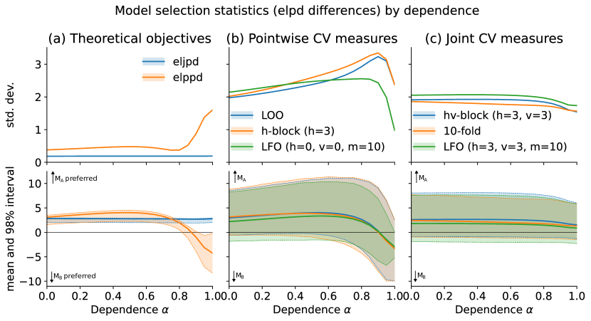
Figure 5: Model selection objectives for the ‘hard’ case ($\beta_{*}=\beta^{\textnormal{hard}}$). Column (a) shows the theoretical model selection objectives, and columns (b) and (c) the associated CV estimates. The top row plots the standard deviation of the relevant $\omega(y)$ for the corresponding column. The bottom row shows its mean and 98% interval. The model parameter $\alpha$ governs the degree of serial dependence. Notice that the adverse selection rate for both joint and pointwise methods is close to zero for all but the strongest dependence. This model selection experiment compares $M_{A}:\operatorname{\mathsf{ARX}\!}\left(1,2\right)$ vs $M_{B}:\operatorname{\mathsf{ARX}\!}\left(1,1\right)$ under an $\operatorname{\mathsf{ARX}\!}\left(2,3\right)$ DGP, as described in Section 4. The autoregressive parameter is $\phi_{*}=\alpha\left(0.75,0.2\right)$, and data length $T$=100. See also Figure 8 for the ‘easy’ case.

Several interesting features of the distribution of $\omega(y)$ are evident in Figure 5, which summarizes the results for the ‘hard’ ($\beta_{*}=\beta_{*}^{\mathrm{hard}}$) case under increasing dependence $\alpha$. These features are consistent with the findings of Section 3. First, notice the striking difference between the behavior of the pointwise and joint theoretical elpds as $\alpha$ increases (column (a)). When data are mutually independent ($\alpha=0$), both distributions are basically equal. For the joint measure, variability and location are little changed as dependence increases. In contrast, the pointwise objective exhibits sharply rising variability and shifts in a negative direction as dependence gains strength. Most of the distribution changes signs entirely to favor the simpler, worse candidate $M_{B}$ as $\alpha$ approaches 1, indicating an adverse selection rate near 100%.

Second, the different profiles exhibited by pointwise and joint CV methods (columns (b) and (c), respectively). While there are clearly differences between the specific joint and pointwise methods, whether the method is computed jointly or pointwise clearly has the greatest bearing on its behavior as dependence increases. The pointwise methods in column (b) exhibit a similar increase in variability and negative shift as the pointwise objective, while the joint methods are little changed as $\alpha\to 1$. In addition, the pointwise CV methods (joint methods too, to a lesser extent) display an interesting decrease in variability as $\alpha$ approaches 1. A possible explanation for this drop-off is the decrease in effective sample size (Berger et al., 2014) for autoregressive models as dependence grows, all else being equal.

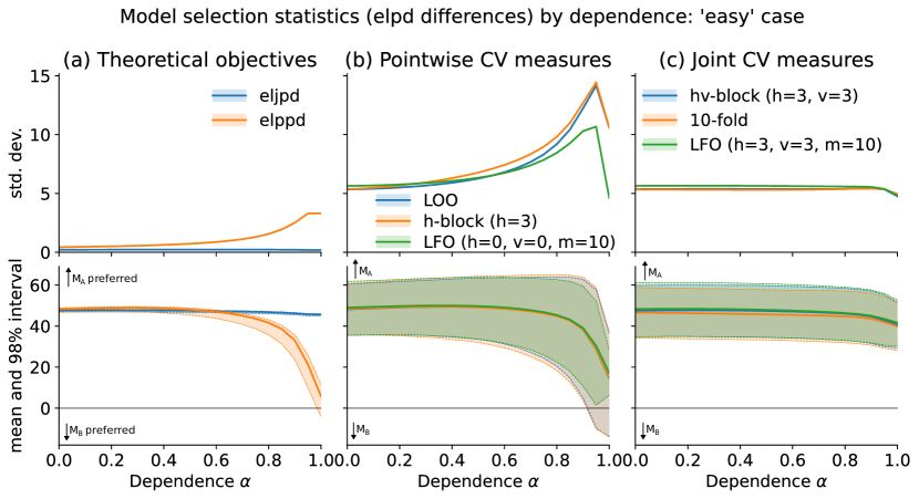
Figure 8: Behavior of model selection objectives for the ‘easy’ case, a counterpoint to Figure 5. Column (a) shows the theoretical model selection objectives, and columns (b) and (c) the associated CV estimates. The top row plots the standard deviation of the relevant $\omega(y)$ for the corresponding column. The bottom row shows its mean and 98% interval. The model parameter $\alpha$ governs the degree of serial dependence. Notice that the adverse selection rate for both joint and pointwise methods is close to zero for all but the strongest dependence. This model selection experiment compares $M_{A}:\operatorname{\mathsf{ARX}\!}\left(1,2\right)$ vs $M_{B}:\operatorname{\mathsf{ARX}\!}\left(1,1\right)$ under an $\operatorname{\mathsf{ARX}\!}\left(2,3\right)$ DGP, as described in Section 4. We use the $\beta^{\textnormal{easy}}$ parameter setting, autoregressive parameter $\phi_{*}=\alpha\left(0.75,0.2\right)$, and data length $T$=100.

Under stronger dependence, increased variability and downward movement together reduce model selection power, consistent with the known bias of CV procedures toward simpler models under small sample sizes. See, for instance Burman (1989) for an analysis of CV bias and sample size. In contrast, for the ‘easy’ experiment variant ($\beta_{*}=\beta_{*}^{\mathrm{easy}}$) where the results are much clearer, cross-validation generates correct model selections for all but the most strongly dependent data (see Figure 8 in Appendix A).

4.4 The cost of an inefficient CV scheme

The distribution of the model selection statistic in Proposition 3 provides a direct method for computing the probability of adverse selection. Noting that a positive selection statistic indicates the correct model choice (corresponding to $M_{A}$), it follows that

$$\Pr\left(\textnormal{adverse selection}\right)=\Pr\left(\omega\left(y\right)<0\right)=F_{\omega\left(y\right)}\!\left(0\right).$$ (4.6)

The quantity $F_{\omega(y)}\!\left(0\right)$ can be interpreted visually in Figure 5 as the share of the $\omega\left(y\right)$ distribution that falls below the $x$-axis. Where the probability of adverse selection is very small we say that the models are well separated under that particular CV scheme. While the infinite support of $\omega\left(y\right)$ means that (4.6) can never be zero, for practical purposes we define a small threshold $\gamma$ as the cutoff for well-separatedness. For the remainder of this paper, we will use $\gamma=0.01$.

Definition 4 (Well-separated).

We say the CV model selection procedure defined above is well-separated at level $\gamma\in\left(0,1\right)$ when $F_{\omega\left(y\right)}\!\left(0\right)<\gamma$.

A particular CV scheme may be well-separated in one situation and poorly separated in another. Whether a model selection procedure is well-separated is determined by all aspects of that procedure, including the details of the data generating process, candidate models, any hyperparameters for the procedure, and the values of the exogenous covariates.

We have seen that an inappropriate choice of CV scheme can result in an elevated probability of adverse selection. In this section, we attempt to quantify this cost.

Perhaps the simplest way to measure the cost of any model selection procedure is the rate of adverse model selection, also known as the ‘0-1 loss’ because it scores all errors equally. The adverse selection rate is the probability (with respect to repeated samples) that the selection procedure will select the wrong model.

Framing the loss as a probability over all realizations of $y$ makes good sense for this paper, since our focus is on the properties of CV methods for $\operatorname{\mathsf{ARX}\!}$ models in general, without reference to a particular data realization $y$. Panels (a) and (b) of Figure 6 compare the adverse selection rate for joint and pointwise CV methods for the ‘hard’ variant of our model selection experiment (losses for the ‘easy’ variant are negligible, and are not shown). The adverse selection rate picks up as $\alpha\to 1$ and for pointwise procedures reaches almost 100 per cent, indicating that CV incorrectly prefers the simpler model when dependence is very strong.

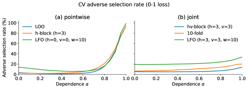
Figure 6: Adverse selection rate for pointwise and joint CV methods as data dependence increases. This experiment compares $M_{A}:\,\operatorname{\mathsf{ARX}\!}\left(1,2\right)$ vs $M_{B}:\,\operatorname{\mathsf{ARX}\!}\left(1,1\right)$, under an $\operatorname{\mathsf{ARX}\!}\left(2,3\right)$ DGP with $\phi_{*}=\alpha\left(0.75,0.2\right)$, for $\alpha\in\left[0,1\right]$ as described in Section 4. Greater values of $\alpha$ denote stronger serial dependence. The ‘hard’ case ($\beta^{\textnormal{hard}}$) with $T=100$ is shown.

The adverse selection rate overlooks a key fact, however: it does not account for the severity of the prediction error, scoring all incorrect selections equally. When there is very little difference between candidates’ model predictions, it matters little which model is chosen. On the other hand, when predictions differ significantly this should be reflected in the cost of the error.

An alternative measure of the cost of adverse selection is the reduction in log utility that results from choosing the incorrect model for a given $y\sim p_{\mathrm{true}}$. Under this formulation, we use the underlying finite-sample theoretical elpd for each $y$ that CV is trying to estimate as the benchmark. This is by its nature a finite-sample loss function.

That is, in the case where CV does not select the elpd-maximizing model we can regard the CV utility cost relative to the counterfactual where the correct model was chosen as the difference between the chosen and maximal elpd:

$$\mathrm{cost}_{CV}\left(y\right)=\max_{M\in\mathcal{M}}\mathrm{elpd}\left(M|y\right)-\mathrm{elpd}\left(M_{CV}^{*}|y\right),$$ (4.7)

where $M_{CV}^{*}=\arg\max_{M\in\mathcal{M}}\widehat{\mathrm{elpd}}_{CV}\left(M|y\right).$

Pointwise elppd and joint eljpd are of course not directly comparable. To put joint and pointwise CV measures on an equal footing, we specify the cost measure measured in terms of joint utility for both pointwise and joint CV procedures,

$$\widetilde{\mathrm{cost}}_{CV}\left(y\right)=\max_{M\in\mathcal{M}}\operatorname{eljpd}\left(M|y\right)-\operatorname{eljpd}\left(M_{CV}^{*}|y\right),$$ (4.8)

where $M_{CV}^{*}=\arg\max_{M\in\mathcal{M}}\widehat{\mathrm{elpd}}_{CV}\left(M|y\right)$ and $\widehat{\mathrm{elpd}}_{CV}\left(\cdot\right)$ can represent either the joint estimate $\widehat{\operatorname{eljpd}}_{CV}\left(\cdot\right)$ or the pointwise estimate $\widehat{\operatorname{elppd}}_{CV}\left(\cdot\right)$.

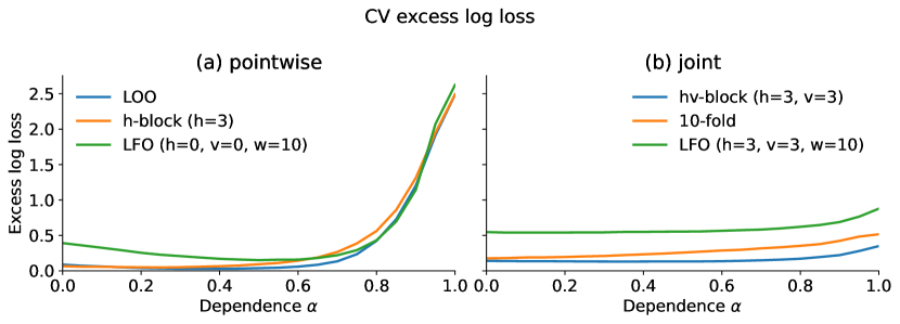
Figure 11: Log loss measures for pointwise and joint CV methods as data dependence increases. This experiment compares $M_{A}:\,\operatorname{\mathsf{ARX}\!}\left(1,2\right)$ vs $M_{B}:\,\operatorname{\mathsf{ARX}\!}\left(1,1\right)$, under an $\operatorname{\mathsf{ARX}\!}\left(2,3\right)$ DGP with $\phi_{*}=\alpha\left(0.75,0.2\right)$, for $\alpha\in\left[0,1\right]$ as described in Section 4. Greater values of $\alpha$ denote stronger serial dependence. T=100. The ‘hard’ model variant ($\beta^{\textnormal{hard}}$) is shown.

Figure 11 in Appendix A plots the log loss defined in the previous display. While excess log loss is an attractive concept, the resulting relative measures are practically indistinguishable from the adverse selection rate. For the remainder of this paper, we will use the adverse selection rate.

4.5 Joint and pointwise objectives

Our results suggest that under dependence, joint estimators usually have lower variability and consequently a lower rate of adverse selection than their pointwise counterparts. In our experiments, these differences are typically negligible for independent observations ($\alpha=0$) and are most pronounced as $\alpha$ approaches 1 and the underlying data become highly persistent. This comparison is quite evident in Figure 6: when $\alpha=0$, joint and pointwise estimators perform roughly equally. As $\alpha\to 1$, there is little change in performance for joint estimators, compared with a dramatic increase in the error rate for the pointwise estimators.

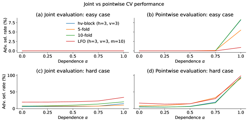
Figure 9: Adverse model selection rates for joint CV methods and structurally identical methods evaluated pointwise. This model selection experiment compares $M_{A}:\operatorname{\mathsf{ARX}\!}\left(1,2\right)$ vs $M_{B}:\operatorname{\mathsf{ARX}\!}\left(1,1\right)$ under an $\operatorname{\mathsf{ARX}\!}\left(2,3\right)$ DGP, as described in Section 4. The ‘easy’ and ‘hard’ results respectively use the $\beta^{\textnormal{easy}}$ and $\beta^{\textnormal{hard}}$ parameter settings. The autoregressive parameter is $\phi_{*}=\alpha\left(0.75,0.2\right)$ and data length $T$=100.

To construct an apples-to-apples comparison between joint and pointwise CV methods, abstracting from other details of the CV scheme design, we construct pointwise analogs to joint designs. For the present experiment this amounts to diagonalizing the covariance matrix of the Gaussian predictive distribution, setting $\sigma_{\ell}^{2}V_{\ell}^{pw}=\sigma_{\ell}^{2}\left(I_{T}\odot V_{\ell}\right)$, for $\odot$ the elementwise product operator. The results confirm a sharp increase in the error rate for pointwise CV methods under strong dependence ($\alpha=1$), compared with almost no difference in the independent case ($\alpha=0$). (See Figure 9 in Appendix A.)

4.6 Specific CV scheme design considerations

We have seen that CV design parameters can have a significant bearing on the overall efficiency, and therefore performance, of CV model selection. In this section we look more closely at hyperparameter choices for specific CV schemes for time-series data.

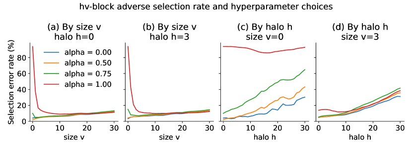
Figure 13: Adverse selection rates using $hv$-block CV with different choices of the halo $h$ and validation set size parameter $v$. Total validation set dimension is $2v+1$. This model selection experiment compares $M_{A}:\operatorname{\mathsf{ARX}\!}\left(1,2\right)$ vs $M_{B}:\operatorname{\mathsf{ARX}\!}\left(1,1\right)$ under a $\operatorname{\mathsf{ARX}\!}\left(2,3\right)$ DGP, as described in Section 4. We use the $\beta^{\textnormal{hard}}$ parameter setting, autoregressive parameter $\phi_{*}=\alpha\left(0.75,0.2\right)$, and data length $T$=100.

Note that $hv$-block CV schemes require the choice of a validation block size $v$ (the total validation set dimension is $2v+1$) and halo size $h$. Consistent with earlier results, for dependent data we find that by far the most important choice is to ensure that $v$ is large enough to capture the dynamic behavior of the model. Either parameter can harm CV performance if it is too large, since both reduce training set size, which imposes a cost on statistical efficiency, resulting in a U-shaped relationship between the adverse selection rate and both $h$ and $v$ when dependence is present. (Figure 13 in Appendix A compares error rates with various choices of these parameters.)

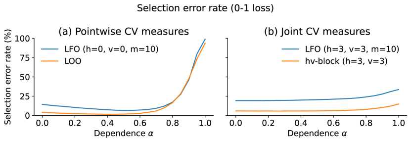
Figure 12: Adverse selection rates for LFO and comparable CV schemes that use future information, by dependence $\alpha$. Notice that in each case, the LFO error rate (blue) exceeds that of the other CV scheme (orange). This model selection experiment compares $M_{A}:\operatorname{\mathsf{ARX}\!}\left(1,2\right)$ vs $M_{B}:\operatorname{\mathsf{ARX}\!}\left(1,1\right)$ under an $\operatorname{\mathsf{ARX}\!}\left(2,3\right)$ DGP, as described in Section 4. We use the $\beta^{\textnormal{hard}}$ parameter setting, autoregressive parameter $\phi_{*}=\alpha\left(0.75,0.2\right)$, and data length $T$=100.

The importance of preserving the size of the training set is evident in the underperformance of LFO, which represents an extreme case for dealing with contamination by discarding the entire future sample. Several authors have pointed out that this is unnecessarily conservative (Bergmeir et al., 2018). Moreover, the analyst should carefully weigh the tradeoff between the bias resulting from the use of future data and the benefit of increasing the training set size. See Figure 12 in Appendix A for a comparison between LFO and methods that use future data. In each case, the adverse selection rate for LFO is substantially higher, a consequence of LFO’s reduced training set size.

4.7 Required sample size

One important practical consequence of an inefficient CV scheme design is that a larger sample size is needed for the models under consideration to be well-separated. This either requires the experimenter to collect more data than is necessary or for the adverse selection rate to be higher than it otherwise would be. In this section we demonstrate that the required sample size increases with dependence, all else being equal. When the underlying process is highly persistent, the required sample size can be significantly larger than for the independent case.

The required sample size for a model to be well-separated goes beyond the well-known principle of the effective sample size (ESS) for a time series model (see e.g. Berger et al., 2014). In this section we demonstrate that properties of the CV procedure—especially whether the scoring rule is evaluated joint or pointwise—strongly determines the data length required.

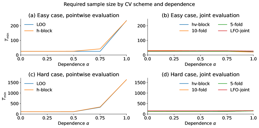
Figure 7: Minimum data length $T$ to be well-separated at the 1% level, found by binary search over the range 10-2500. This model selection experiment compares $M_{A}:\operatorname{\mathsf{ARX}\!}\left(1,2\right)$ vs $M_{B}:\operatorname{\mathsf{ARX}\!}\left(1,1\right)$ under an $\operatorname{\mathsf{ARX}\!}\left(2,3\right)$ DGP, as described in Section 4. The DGP autoregressive parameter is $\phi_{*}=\alpha\left(0.75,0.2\right)$. See also Figure 10 in Appendix A.

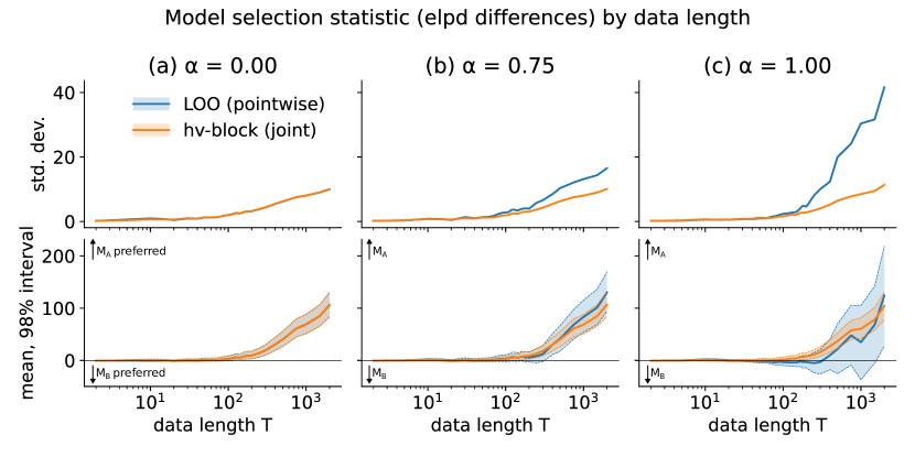
Figure 10: CV model selection statistic variability by data length $T$ for LOO-CV and $hv$-block CV. The degree of data dependence increases across columns from left to right. The top row shows the model selection statistic standard deviation and the bottom row its 98% probability interval. This model selection experiment compares $M_{A}:\operatorname{\mathsf{ARX}\!}\left(1,2\right)$ vs $M_{B}:\operatorname{\mathsf{ARX}\!}\left(1,1\right)$ under a $\operatorname{\mathsf{ARX}\!}\left(2,3\right)$ dgp, as described in Section 4. We use the $\beta^{\textnormal{hard}}$ parameter setting, autoregressive parameter $\phi_{*}=\alpha\left(0.75,0.2\right)$, and data length $T$=100.

Figure 7 compares the minimum sample size required for several more joint and pointwise CV methods. Consistent with earlier results, there is little difference required sample size between pointwise and joint methods in the independent case ($\alpha=0$). Under stronger dependence, however, the greater variability of pointwise methods leads to a requirement for larger sample sizes for the two candidate models to be well-separated, all else being equal. These results underscore the importance of using efficient CV designs—especially the use of joint scoring rules—when strong dependence is present. See also Figure 10 in Appendix A.

As we might expect, the benefit of using more efficient CV methods is greatest when candidate models are more challenging to separate. In Figure 7, required sample size is greatest for the ‘hard’ variant, especially under a high degree of dependence. In comparison, under the ‘easy’ variant the differences between joint and pointwise methods are smaller, although there is nonetheless a pickup in the sample size required for pointwise CV methods.

Figure 7 also underscores the benefit of using as much of the available sample as possible, rather than discarding future observations as in LFO methods. As dependence increases, the additional statistical efficiency associated with allowing the model to learn from future data results in a well-separated model with shorter overall data lengths.

5 Discussion and conclusion

We have demonstrated that in settings where serial dependence is present, appropriate CV procedure design can dramatically improve model selection performance. Working with the logarithmic scoring rule and the $\operatorname{\mathsf{ARX}\!}(p,q)$ class of autoregressive models, we have shown that evaluating the score pointwise can yield highly inefficient CV estimators that perform poorly when compared with procedures that target joint densities. Our experiments show that pointwise CV estimators exhibit greater variability and require larger sample sizes than joint designs.

We are not the first to compare the performance between joint and pointwise densities in predictive model assessment. Osband et al. (2022), for instance, apply model assessment with joint densities in the context of neural networks.

Our results show that the consequences of using an inefficient CV procedure can be particularly pernicious under strong serial dependence. One consequence is that CV procedures become biased toward overly simple models. In extreme cases where serial dependence is greatest, this can result in different CV procedures assigning completely different orderings to candidate models. Viewed another way, the consequence of the use of inappropriate CV procedures is the need for larger sample sizes to achieve good separation between models.

Relatively conservative methods like LFO can be a good choice in applied contexts, especially when CV is able to clearly separate models even without the use of the full sample for reducing estimator variability. Furthermore, some authors have advocated for the use of LFO (e.g., Bürkner et al., 2020) when the dependence structure is unknown. While LFO certainly eliminates the possibility that contamination will bias results, the results of Section 4.6 suggest that contamination arising from the use of future data and training set size does need to be carefully traded off against the benefit of retaining a larger training set. In general, it seems unlikely that the optimal CV design would be the corner solution that excludes all future observations. Risks associated with contamination can also be avoided by the use of specification tests on candidate models before conducting model comparison, including standard Bayesian model criticism procedures and testing for autocorrelation in the residuals (Bergmeir et al., 2018). Model assessment is especially important when the underlying process is highly persistent. Not only is the need for larger effective sample sizes greatest under persistence processes, but the adverse impact of contamination is most pernicious.

Our goal throughout this paper has been model selection. We are not claiming that exploiting future observations in CV schemes yields nearly unbiased estimators of the elpd. Instead, here we are targeting relative measures that are efficient model selection objectives.

This analysis has focused on serial dependence, which most often appears in time series models. However, we expect that similar results would apply for other forms of dependence such as spatial and spatio-temporal data, especially where the autoregressive signal is relatively strong compared with the global conditional mean. Naturally, dependence structures in more than one dimension presents additional analytical challenges, so further research is warranted for these and other dependence structures. Furthermore, many of our conclusions are not specific to the logarithmic score and would also apply under other scoring rules (Gneiting and Raftery, 2007).

From a practical standpoint, it should be noted that implementing joint CV methods tends to be computationally costly when compared with pointwise procedures like LOO. In situations where the difference between two models is absolutely clear, as for the ‘easy’ variant of our examples under weak serial dependence, pointwise CV estimators may be adequate for performing model selection and are far more convenient to construct. This is particularly relevant considering the availability of efficient computational shortcuts for computing pointwise CV procedures, such as PSIS-LOO (Vehtari et al., 2017; Bürkner et al., 2020), and a lack of similar shortcuts for joint procedures. Although in principle PSIS-LOO can also approximate joint CV procedures, in practice the thick tails of the weight distributions tend to cause importance sampling to fail.

With the complexity of implementing joint procedures in mind, we recommend the following workflow for model selection under serial dependence. Begin with a thorough model criticism of each of the candidate models, and iterate model specification until the candidate models are well-specified. Where inference results show that serial dependence is relatively weak, pointwise CV methods such as PSIS-LOO can be used as a first pass for model selection. If the pointwise CV results show a clear preference for one candidate, then that candidate can be selected. Otherwise, a joint CV procedure should be implemented and relied upon instead.

The present paper represents a first look at the uncertainty of CV-based model selection under serial dependence, but there is considerable work remaining. We have focused on identification of the regression parameter, leaving to one side the tasks of identifying the autoregressive component, theoretical analysis of these results, choosing suitable priors for model identification procedures, and constructing efficient computational methods for CV under serial dependence. We leave these aspects for future work.

Appendixes This supplement contains additional plots and tables referenced in the main text. The supplement also contains derivations and proofs to support the experiments in the paper.

[Acknowledgments] The authors are grateful for the input of two anonymous referees and an associate editor. Any remaining errors are our own. AC’s work was supported in part by an Australian Government Research Training Program Scholarship. AV acknowledges the Academy of Finland Flagship program: Finnish Center for Artificial Intelligence, and Academy of Finland project (340721). CF acknowledges financial support under National Science Foundation Grant SES-1921523. LK gratefully recognises support from the National Institutes of Health (5R01AG067149-02).

Appendix A Additional plots

This section contains supplementary plots referenced in the main text.

Appendix B Supplementary experiments

The extended example described in Section 4 is a model selection experiment comparing $M_{A}:\,\operatorname{\mathsf{ARX}\!}\left(1,2\right)$ vs $M_{B}:\,\operatorname{\mathsf{ARX}\!}\left(1,1\right)$, where the data are generated by an $\operatorname{\mathsf{ARX}\!}\left(2,3\right)$ DGP. We chose this experiment and the associated parameter vectors $\beta_{*}^{\textnormal{easy}}$ and $\beta_{*}^{\textnormal{hard}}$ because we believe they are representative of typical CV problems faced in experimental settings—that is, neither $M_{A}$ nor $M_{B}$ have the same functional form as the DGP, but one is clearly a better fit than the other.

This appendix presents the results of additional experiments using other models from the $\operatorname{\mathsf{ARX}\!}$ class. The goal of these supplementary results is to demonstrate that the main experiment is representative of typical cases, and to highlight specific cases where behaviors can differ. For consistency and simplicity we retain the same values for the parameter vectors $\beta_{*}^{\textnormal{easy}}$ and $\beta_{*}^{\textnormal{hard}}$. We choose $LOO$ as an example of a pointwise CV method and $hv-\mathrm{block}(3,3)$ as an example of a joint CV method. In each case the focus is on identifying the regression parameter, so each candidate model has the same autoregressive structure.

Let the stationary vector $y=y_{1},\dots,y_{T}$ be distributed according to an $\operatorname{\mathsf{ARX}\!}\left(p_{*},q_{*}\right)$ of the form,

$$\textnormal{DGP}:\ y_{t}=\phi_{*}^{\top}\begin{pmatrix}y_{t-1}\\ \vdots\\ y_{t-p^{*}}\end{pmatrix}+\beta_{*}^{\top}z_{t}+\sigma_{*}\varepsilon_{t},$$ (B.1)

where $\varepsilon_{t}\overset{\mathrm{iid}}{\sim}\mathcal{N}\left(0,1\right)$. The experiment selects between two candidate models,

$$M_{A}:\ y_{t} =\widehat{\phi_{A}}\begin{pmatrix}y_{t-1}\\ \vdots\\ y_{t-p_{A}}\end{pmatrix}+\beta_{A}^{\top}z_{t}+\widehat{\sigma_{A}}\varepsilon_{t} \operatorname{\mathsf{ARX}\!}\left(p_{A},q_{A}\right)$$ (B.2)

$$M_{B}:\ y_{t} =\widehat{\phi_{B}}\begin{pmatrix}y_{t-1}\\ \vdots\\ y_{t-p_{B}}\end{pmatrix}+\beta_{B}^{\top}z_{t}+\widehat{\sigma_{B}}\varepsilon_{t} \operatorname{\mathsf{ARX}\!}\left(p_{B},q_{B}\right).$$ (B.3)

Table 1 lists the additional experiments. In each case, the DGP is parameterized by $\alpha\in\left[0,1\right]$, which controls the degree of dependence. Each experiment is run twice, once each with $\beta_{*}^{\textnormal{easy}}$ and $\beta_{*}^{\textnormal{hard}}$. The DGP parameter $\alpha\in\left[0,1\right]$ is varied to select the degree of serial dependence. All DGPs are stationary. The random noise component is distributed as $\varepsilon_{t}\overset{iid}{\sim}N\left(0,1\right)$, the fixed per-period covariates $z_{1t}$ and $z_{2t}$ are drawn independently from the standard normal distribution, and priors are $\beta_{i}\sim\mathcal{N}\left(\beta_{*i},1\right)$, for $i=1,2,3$. Initial values are $y_{t}=0$ for $t\leq 0$. For all examples in this section, the data length is $T=100$. As in Section 4, we solve (4.3) to find optimal noise variance and autoregressive parameter values.

The results of the additional experiments are broadly similar to Experiment 1: joint and pointwise methods perform similarly under no dependence, and under stronger dependence both the variability and error rates of the pointwise estimators are higher than that of the joint estimators. Experiment 4, for which the candidate models both have no autoregressive component at all, is an exception, and both methods perform terribly under strong dependence. It should perhaps not be surprising that such badly misspecified models would perform so poorly, which underscores the need for thorough model criticism for all candidates before conducting CV.

Primary experiment (main text)
#	DGP and candidate models
1.	$\operatorname{\mathsf{ARX}\!}\left(2,3\right)\,\mathrm{DGP}:y_{t}=\alpha\begin{pmatrix}0.75\\ 0.2\end{pmatrix}^{\top}\begin{pmatrix}y_{t-1}\\ y_{t-2}\end{pmatrix}+\beta_{*1}+\beta_{*2}z_{2t}+\beta_{*3}z_{3t}+\varepsilon_{t}$
	$\operatorname{\mathsf{ARX}\!}\left(1,2\right)\,M_{A}:y_{t}=\phi_{1}y_{t-2}+\beta_{1}+\beta_{2}z_{2t}+\varepsilon_{t}$
	$\operatorname{\mathsf{ARX}\!}\left(1,1\right)\,M_{B}:y_{t}=\phi_{1}y_{t-1}+\beta_{1}+\varepsilon_{t}$
Supplementary experiments (this appendix)
#	DGP and candidate models
2.	$\operatorname{\mathsf{ARX}\!}\left(1,3\right)\,\mathrm{DGP}:y_{t}=\alpha\left(0.95\right)y_{t-1}+\beta_{*1}+\beta_{*2}z_{2t}+\beta_{*3}z_{3t}+\varepsilon_{t}$
	$\operatorname{\mathsf{ARX}\!}\left(1,3\right)\,M_{A}:y_{t}=\phi_{1}y_{t-1}+\beta_{1}+\beta_{2}z_{2t}+\beta_{3}z_{3t}+\varepsilon_{t}$
	$\operatorname{\mathsf{ARX}\!}\left(1,2\right)\,M_{B}:y_{t}=\phi_{1}y_{t-1}+\beta_{1}+\beta_{2}z_{2t}+\varepsilon_{t}$
3.	$\operatorname{\mathsf{ARX}\!}\left(1,3\right)\,\mathrm{DGP}:y_{t}=\alpha\left(0.95\right)y_{t-1}+\beta_{*1}+\beta_{*2}z_{2t}+\beta_{*3}z_{3t}+\varepsilon_{t}$
	$\operatorname{\mathsf{ARX}\!}\left(1,2\right)\,M_{A}:y_{t}=\phi_{1}y_{t-1}+\beta_{1}+\beta_{2}z_{2t}+\varepsilon_{t}$
	$\operatorname{\mathsf{ARX}\!}\left(1,1\right)\,M_{B}:y_{t}=\phi_{1}y_{t-1}+\beta_{1}+\varepsilon_{t}$
4.	$\operatorname{\mathsf{ARX}\!}\left(1,3\right)\,\mathrm{DGP}:y_{t}=\alpha\left(0.95\right)y_{t-1}+\beta_{*1}+\beta_{*2}z_{2t}+\beta_{*3}z_{3t}+\varepsilon_{t}$
	$\operatorname{\mathsf{ARX}\!}\left(0,2\right)\,M_{A}:y_{t}=\beta_{1}+\beta_{2}z_{2t}+\varepsilon_{t}$
	$\operatorname{\mathsf{ARX}\!}\left(0,1\right)\,M_{B}:y_{t}=\beta_{1}+\varepsilon_{t}$
5.	$\operatorname{\mathsf{ARX}\!}\left(2,3\right)\,\mathrm{DGP}:y_{t}=\alpha\begin{pmatrix}0.75\\ 0.2\end{pmatrix}^{\top}\begin{pmatrix}y_{t-1}\\ y_{t-2}\end{pmatrix}+\beta_{*1}+\beta_{*2}z_{2t}+\beta_{*3}z_{3t}+\varepsilon_{t}$
	$\operatorname{\mathsf{ARX}\!}\left(1,3\right)\,M_{A}:y_{t}=\phi_{1}y_{t-1}+\beta_{1}+\beta_{2}z_{2t}+\beta_{3}z_{3t}+\varepsilon_{t}$
	$\operatorname{\mathsf{ARX}\!}\left(1,1\right)\,M_{B}:y_{t}=\phi_{1}y_{t-2}+\beta_{1}+\varepsilon_{t}$

Table 1: Additional model selection experiments. Experiment 1 corresponds to the DGP and candidate models in Section 4. Each experiment in this Appendix compares two commonly-deployed CV methods: LOO (which has a univariate scoring rule, hence evaluated pointwise), and $hv$-block CV with $h=3$ and $v=3$, evaluated jointly.

Supplementary experiments: adverse selection rates
Probability of adverse selection (%)
		‘Easy’ variant $\left(\beta^{\textnormal{easy}}\right)$					‘Hard’ variant $\left(\beta^{\textnormal{hard}}\right)$
		$\alpha$					$\alpha$
		$0$	$\frac{1}{2}$	$\frac{3}{4}$	$1$		$0$	$\frac{1}{2}$	$\frac{3}{4}$	$1$
Experiment 1
LOO		0.0	0.0	0.0	9.1		4.1	1.8	10.1	93.9
$hv$-block(3,3)		0.0	0.0	0.0	0.0		5.9	6.0	7.3	14.8
Experiment 2
LOO		0.0	0.0	0.0	1.5		0.0	0.0	0.0	1.0
$hv$-block(3,3)		0.0	0.0	0.0	0.0		0.0	0.0	0.0	0.0
Experiment 3
LOO		0.0	0.0	0.0	2.5		4.1	1.5	8.7	82.9
$hv$-block(3,3)		0.0	0.0	0.0	0.0		5.9	4.8	4.6	7.8
Experiment 4
LOO		0.0	0.0	0.0	85.7		4.5	6.3	28.8	98.5
$hv$-block(3,3)		0.0	0.0	0.0	92.8		5.0	8.6	32.9	98.7
Experiment 5
LOO		0.0	0.0	0.0	0.2		0.0	0.0	0.0	0.1
$hv$-block(3,3)		0.0	0.0	0.0	0.0		0.0	0.0	0.0	0.0

Table 2: Adverse selection rates for experiments in Table 1.

Supplementary experiments: variability
Model selection statistic standard deviation
		‘Easy’ variant $\left(\beta^{\textnormal{easy}}\right)$					‘Hard’ variant $\left(\beta^{\textnormal{hard}}\right)$
		$\alpha$					$\alpha$
		$0$	$\frac{1}{2}$	$\frac{3}{4}$	$1$		$0$	$\frac{1}{2}$	$\frac{3}{4}$	$1$
Experiment 1
LOO		5.35	6.26	8.32	10.59		1.98	2.38	2.78	2.37
$hv$-block(3,3)		5.36	5.37	5.38	4.77		1.91	1.92	1.88	1.54
Experiment 2
LOO		6.13	7.68	9.99	11.76		6.11	7.54	9.59	10.46
$hv$-block(3,3)		6.07	6.23	6.33	5.89		6.06	6.19	6.27	5.81
Experiment 3
LOO		5.35	6.47	8.74	10.90		1.98	2.50	3.02	2.83
$hv$-block(3,3)		5.36	5.38	5.42	5.02		1.91	1.98	2.00	1.75
Experiment 4
LOO		0.0	0.0	0.0	85.7		4.5	6.3	28.8	98.5
$hv$-block(3,3)		0.0	0.0	0.0	92.8		5.0	8.6	32.9	98.7
Experiment 5
LOO		7.04	7.86	9.60	11.23		6.27	7.32	8.72	6.60
$hv$-block(3,3)		7.04	6.97	6.87	6.12		6.19	6.16	6.05	5.24

Table 3: CV model selection statistic standard deviation for experiments in Table 1.

Appendix C Autoregressive dependence

Start with an $\operatorname{\mathsf{ARX}\!}(p,q)$ with common noise variance $\sigma^{2}>0$, where

$$y_{t}\,|\,y_{\left(t-p\right):\left(t-1\right)},\phi,\sigma^{2}\sim\mathcal{N}\left(\sum_{i=1}^{p}\phi_{i}y_{t-i}+z_{t}^{\top}\beta,\sigma^{2}\right),\quad t=1,\dots,T.$$ (C.1)

We denote $y_{r:s}=\left(y_{r},y_{r+1},\dots,y_{s-1},y_{s}\right).$ For simplicity, we will fix the $p$ initial values $y_{0}=\dots=y_{1-p}=0$,

$$y_{t}\,|\,y_{\mathrm{max}\left(1,t-p\right):\left(t-1\right)},\phi,\sigma^{2}\sim\mathcal{N}\left(\sum_{i=1}^{\mathrm{min}\left(p,t-1\right)}\phi_{i}y_{t-i}+z_{t}^{\top}\beta,\sigma^{2}\right),\quad t=1,\dots,T.$$ (C.2)

It follows that the joint distribution of the vector $y$ is multivariate normal, as summarized by Lemma 5.

Lemma 5.

Let $y=\left(y_{1},\dots,y_{T}\right)$ be distributed according to (C.2) with $y_{0}=\dots=y_{1-p}=0$. Then its joint density is multivariate normal,

$$y\ |\ \phi,\beta,\sigma^{2}\sim\mathcal{N}\left(L_{\phi}^{-1}Z\beta,\sigma^{2}W_{\phi}\right),$$ (C.3)

where the $T\times T$ covariance matrix $W_{\phi}=\left(L_{\phi}^{\top}L_{\phi}\right)^{-1}$ is positive definite with $\left|W_{\phi}\right|=1$. The $T\times T$ banded lower triangular coefficient matrix $L_{\phi}$ has entries

$$\left(L_{\phi}\right)_{s,t}=\begin{cases}1&\textnormal{for }s=t\\ -\phi_{s-t}&\textnormal{for }1\leq s-t\leq p\\ 0&\textnormal{otherwise}.\end{cases}$$ (C.4)

Proof.

First note that $L_{\phi}$ is lower-triangular with $1$s on the diagonal, so $\left|L_{\phi}\right|=1$ and the inverse $L_{\phi}^{-1}$ exists. The $T\times 1$ vector $\eta$ with $t$th entry

$$\eta_{t}=y_{t}-\sum_{i=1}^{p}\boldsymbol{1}\!\left\{t-i\geq 1\right\}\phi_{i}y_{t-i}-z_{t}^{\top}\beta$$ (C.5)

can equivalently be written in vector form as $\eta=L_{\phi}y-Z\beta$, where $Z$ is the matrix with rows $\left(z_{t}^{\top}\right)$ and $\boldsymbol{1}\!\left\{\cdot\right\}$ is the indicator function. Then, the joint density of $y$ is

$$p\left(y\,|\,\phi,\beta,\sigma^{2}\right) =p\left(y_{1}\,|\,\phi,\beta,\sigma^{2}\right)\prod_{t=2}^{T}p\left(y_{t}\,|\,y_{\mathrm{max}\left(1,t-p\right):\left(t-1\right)},\phi,\beta,\sigma^{2}\right)$$ (C.6)

$$=\left(2\pi\sigma^{2}\right)^{-T/2}\exp\left\{-\frac{1}{2\sigma^{2}}\eta^{\top}\eta\right\}$$ (C.7)

$$=\left(2\pi\sigma^{2}\right)^{-T/2}\exp\left\{-\frac{1}{2\sigma^{2}}\left(L_{\phi}y-Z\beta\right)^{\top}\left(L_{\phi}y-Z\beta\right)\right\}$$ (C.8)

$$=\left(2\pi\sigma^{2}\right)^{-T/2}\exp\left\{-\frac{1}{2\sigma^{2}}\left(y-L_{\phi}^{-1}Z\beta\right)^{\top}L_{\phi}^{\top}L_{\phi}\left(y-L_{\phi}^{-1}Z\beta\right)\right\}$$ (C.9)

$$=\mathcal{N}\left(y\,|\,L_{\phi}^{-1}Z\beta,\sigma^{2}W_{\phi}\right),$$ (C.10)

as required. To see that $W_{\phi}$ is positive definite, recognize that $\left|W_{\phi}\right|=\left|L_{\phi}\right|^{-2}=1$, completing the proof. ∎

Note that the matrix $L_{\phi}$ is not the Cholesky factor of $V_{\phi}^{-1}$. Recall that the lower-left Cholesky factor $A$ for $V_{\phi}^{-1}$ is the unique solution to $AA^{\top}=V_{\phi}^{-1}$. In contrast, we have $L_{\phi}^{\top}L_{\phi}=V_{\phi}^{-1}$.

Appendix D Simplified model

This section derives the simplified $\operatorname{\mathsf{ARX}\!}(p,q)$ model examined in Section 4.

To abstract away the details of particular CV blocking schemes, in mathematical expressions we will use selection matrixes to construct subvectors of the training data $y$ and replicate data vector $\tilde{y}$, as well as parameters of marginal distributions. Consider first just a single CV fold. Let the ordered sets $\mathsf{train}$ and $\mathsf{test}$ be subsets of $\left\{1,2,\cdots,T\right\}$, retaining only the indexes of the desired test and training subsets. For CV estimators, $\mathsf{train}$ and $\mathsf{test}$ are mutually disjoint. Define the $n\times T$ matrix $\mathring{S}$ and $v\times T$ matrix $\tilde{S}$ such that $y_{\mathsf{train}}=\mathring{S}y$ and $\tilde{y}_{\mathsf{test}}=\tilde{S}\tilde{y}$. The elements of $\mathring{S}$ and $\tilde{S}$ are given by

$$\left(\mathring{S}\right)_{j,t}:=\boldsymbol{1}\!\left\{t=\mathsf{train}{}_{j}\right\}\quad\textnormal{and}\quad\left(\tilde{S}\right)_{k,t}:=\boldsymbol{1}\!\left\{t=\mathsf{test}{}_{\ell}\right\},$$ (D.1)

where $\boldsymbol{1}\!\left\{\cdot\right\}$ denotes the indicator function, $\mathsf{train}{}_{j}$ and $\mathsf{test}{}_{k}$ respectively denote the $j$th and $k$th elements of $\mathsf{train}$ and $\mathsf{test}$, $t=1,\cdots,T$, $j=1,\cdots,n$, and $k=1,\cdots,v$.

D.1 Posterior and predictive distributions

Lemma 5 and (2.1) imply that the model for $y$ given $\phi$, $\beta$, and $\sigma^{2}$ can be written as

$$p\left(y_{\mathsf{train}}\,|\,\phi,\beta,\sigma^{2}\right)=\mathcal{N}\left(\mathring{S}y\,|\,\mathring{S}L_{\phi}^{-1}Z\beta,\sigma^{2}\mathring{S}W_{\phi}\mathring{S}^{\top}\right)$$ (D.2)

where $y=\left(y_{1},y_{2},\dots,y_{T}\right)$ and $y_{\mathsf{train}}=\mathring{S}y$ by definition. The $T\times q$ matrix of exogenous regressors $Z$ includes a column of ones, and the $T\times T$ lower-triangular coefficient matrix $L_{\phi}$ is as defined in (C.4).

We require the posterior density conditional on fixed values for $\phi$ and $\sigma^{2}$, which we define in Section 4.2, below. The posterior density can be derived analytically in the usual way for models with conjugate priors, as proportional to the joint density,

$$p\left(\beta\,|\,y_{\mathsf{train}},\sigma^{2},\phi\right) \propto p\left(y_{\mathsf{train}}\,|\,\beta,\sigma^{2},\phi\right)p\left(\beta\right)$$ (D.3)

$$=\mathcal{N}\left(\mathring{S}y\,|\,\mathring{S}L_{\phi}^{-1}Z\beta,\sigma^{2}\mathring{S}W_{\phi}\mathring{S}^{\top}\right)\mathcal{N}\left(\beta\,|\,\mu_{\beta},\sigma^{2}\Sigma_{\beta}\right)$$ (D.4)

$$\propto\exp\left\{-\frac{1}{2\sigma^{2}}\left(\beta-\Sigma_{\beta}\mu_{\beta}\right)^{\top}\Sigma_{\beta}^{-1}\left(\beta-\Sigma_{\beta}\mu_{\beta}\right)\right\}.$$ (D.5)

In the above, we have completed the square and defined

$$\Sigma_{\beta} =\left[Z^{\top}L_{\phi}^{-\top}\mathring{S}^{\top}\left(\mathring{S}W_{\phi}\mathring{S}^{\top}\right)^{-1}\mathring{S}L_{\phi}^{-1}Z+\Sigma_{0}^{-1}\right]^{-1}$$ (D.6)

$$\mu_{\beta} =\Sigma_{\beta}\left[Z^{\top}L_{\phi}^{-\top}\mathring{S}^{\top}\left(\mathring{S}W_{\phi}\mathring{S}^{\top}\right)^{-1}\mathring{S}y+\Sigma_{0}^{-1}\mu_{0}\right].$$ (D.7)

In the case where the full training set is used so that $\mathring{S}=I_{T}$, we can exploit the fact that $W_{\phi}^{-1}=L_{\phi}^{\top}L_{\phi}$ to simplify (D.6) as $\Sigma_{\beta}=\left(Z^{\top}Z+\Sigma_{0}^{-1}\right)^{-1}$.

The resulting model $M_{\ell}$ posterior density for $\beta$ (conditional on $\sigma^{2}$ and $\phi$) is multivariate normal,

$$p\left(\beta\,|\,y_{\mathsf{train}},\sigma^{2},\phi\right) =\mathcal{N}\left(\beta\,|\,\mu_{\beta},\sigma^{2}\Sigma_{\beta}\right).$$ (D.8)

The posterior predictive density for new data $\tilde{y}_{test}=\tilde{S}\tilde{y}$ can be derived by integrating out the parameter $\beta$ from the joint distribution of new data and $\beta$ given $y_{\mathsf{train}}$,

$$p\left(\tilde{y}_{\mathsf{test}}|y_{\mathsf{train}},\sigma^{2},\phi\right)$$

$$=\int p\left(\tilde{y}_{\mathsf{test}}\,|\,\beta,\sigma^{2},\phi\right)p\left(\beta\,|\,y_{\mathsf{train}},\sigma^{2},\phi\right)\mathrm{d}\beta$$ (D.9)

$$=\int\mathcal{N}\left(\tilde{S}y\,|\,\tilde{S}L_{\phi}^{-1}Z_{\ell}\beta,\sigma^{2}\tilde{S}W_{\phi}\tilde{S}^{\top}\right)\mathcal{N}\left(\beta\,|\,\mu_{\beta},\sigma^{2}\Sigma_{\beta}\right)\mathrm{d}\beta$$ (D.10)

$$=\mathcal{N}\Bigl{(}\tilde{S}\tilde{y}\,|\,\tilde{S}\underbrace{L_{\phi}^{-1}Z_{\ell}\mu_{\beta}}_{m_{\ell}},\sigma^{2}\tilde{S}\Bigl{(}\underbrace{W_{\phi}+L_{\phi}^{-1}Z_{\ell}\Sigma_{\beta}Z_{\ell}^{\top}L_{\phi}^{-\top}}_{V_{\ell}}\Bigr{)}\tilde{S}^{\top}\Bigr{)}.$$ (D.11)

It is worth emphasizing that in our framework the DGP (3.1) and model $M_{\ell}$ can represent different underlying models. In other words, we allow $M_{\ell}$ to be misspecified. This means that the theoretical and cross-validatory utility measures will be a function of both the DGP parameters (with $*$ subscripts) and the model $M_{\ell}$ parameters (with $\ell$ subscripts).

D.2 Theoretical expected log predictive density

The theoretical log utility under external validation (2.3) is simply the expectation of the log predictive density under the true DGP. In the simplified version of the model, both the DGP and predictives are multivariate Gaussian and an exact solution is available analytically as a consequence of Lemma 8 (Appendix F). Sivula et al. (2020) found that the $\operatorname{elppd}$ for linear regressions with flat priors can be expressed as a second-degree polynomial in $y$. We find that this is also true for both the $\operatorname{eljpd}$ and $\operatorname{elppd}$ for our simplified $\operatorname{\mathsf{ARX}\!}$ model with conjugate priors.

D.2.1 Expected log joint predictive density (eljpd)

We will derive the $\operatorname{eljpd}$ in a form that includes selection matrixes for both testing and training data. This form is general enough that it can be used to analyze full-data $\operatorname{elpd}$s as well as to construct cross-validation folds with subsets of the data. Let the selection matrixes $\mathring{S}$ and $\tilde{S}$ respectively define the training and testing subsets of $y$ and $\tilde{y}$. Then, dropping the conditioning $\sigma^{2}$ and $\phi$ from the notation for brevity, the joint theoretical utility for model $M_{\ell}$ given $y$ is,

$$\operatorname{eljpd}\left(M_{\ell}\,|\,y,\tilde{S}\right)$$

$$=\mathbb{E}_{\tilde{y}_{\mathsf{test}}\sim p_{\mathrm{true}}}\left[\log p\left(\tilde{y}_{\mathsf{test}}\,|\,y_{\mathsf{train}},M_{\ell}\right)\right]$$ (D.12)

$$=\int\mathcal{N}\left(\tilde{S}\tilde{y}\,|\,\tilde{S}m_{*},\sigma_{*}^{2}\tilde{S}V_{*}\tilde{S}^{\top}\right)\log\mathcal{N}\left(\tilde{S}\tilde{y}\,|\,\tilde{S}m_{\ell},\sigma_{\ell}^{2}\tilde{S}V_{\ell}\tilde{S}^{\top}\right)\,\mathrm{d}\tilde{y}$$ (D.13)

$$=-\frac{1}{2}\Biggl{\{}\log\left|2\pi\sigma_{\ell}^{2}\tilde{S}V_{\ell}\tilde{S}^{\top}\right|+\frac{\sigma_{*}^{2}}{\sigma_{\ell}^{2}}\mathrm{tr}\left[\left(\tilde{S}V_{\ell}\tilde{S}^{\top}\right)^{-1}\tilde{S}V_{*}\tilde{S}^{\top}\right]$$

$$\qquad+\left(m_{\ell}-m_{*}\right)^{\top}\tilde{S}^{\top}\left(\sigma_{\ell}^{2}\tilde{S}V_{\ell}\tilde{S}^{\top}\right)^{-1}\tilde{S}\left(m_{\ell}-m_{*}\right)\Biggr{\}}$$ (D.14)

where we have used (E.1) and (D.11) and Lemma 8. Now note that $m_{\ell}$ is linear in $y$,

$$m_{\ell} =L_{\phi}^{-1}Z_{\ell}\mu_{\beta}=D_{\ell}y+e_{\ell}$$ (D.15)

where we have used (D.2) to define

$$D_{\ell} =L_{\phi_{\ell}}^{-1}Z_{\ell}\Sigma_{\beta_{\ell}}Z_{\ell}^{\top}L_{\phi_{\ell}}^{-\top}\mathring{S}^{\top}\left(\mathring{S}W_{\phi}\mathring{S}^{\top}\right)^{-1}\mathring{S},$$ (D.16)

$$e_{\ell} =L_{\phi_{\ell}}^{-1}Z_{\ell}\Sigma_{\beta_{\ell}}\Sigma_{0}^{-1}\mu_{0}.$$ (D.17)

Observe that in the case where the full training set is used ($\mathring{S}=I_{T}$), we can use the fact that $W_{\phi}^{-1}=L_{\phi}^{\top}L_{\phi}$ to simplify $D_{\ell}=L_{\phi_{\ell}}^{-1}Z_{\ell}\Sigma_{\beta_{\ell}}Z_{\ell}^{\top}L_{\phi_{\ell}}.$

Finally, rearranging (D.14) and substituting (D.15) yields the second-degree polynomial in $y$,

$$\operatorname{eljpd}\left(M_{\ell}\,|\,y,\tilde{S}\right) =y^{\top}A_{\ell}y+y^{\top}b_{\ell}+c_{\ell}.$$ (D.18)

The $T\times T$ matrix $A_{\ell}$, $T\times 1$ vector $b_{\ell}$, and scalar $c_{\ell}$ are nonlinear functions of $\phi_{*}$ and $\phi_{\ell}$ (respectively via $V_{*}$ and $V_{\ell}$) but are free of $y$ and hence nonrandom. Their values are

$$A_{\ell} =-\frac{1}{2\sigma_{\ell}^{2}}D_{\ell}^{\top}\tilde{S}^{\top}\left(\tilde{S}V_{\ell}\tilde{S}^{\top}\right)^{-1}\tilde{S}D_{\ell}$$ (D.19)

$$b_{\ell} =-\frac{1}{\sigma_{\ell}^{2}}D_{\ell}^{\top}\tilde{S}^{\top}\left(\tilde{S}V_{\ell}\tilde{S}^{\top}\right)^{-1}\tilde{S}\left(e_{\ell}-m_{*}\right)$$ (D.20)

$$c_{\ell} =-\frac{1}{2}\log\left|2\pi\sigma_{\ell}^{2}\tilde{S}V_{\ell}\tilde{S}^{\top}\right|-\frac{\sigma_{*}^{2}}{2\sigma_{\ell}^{2}}\mathrm{tr}\left[\left(\tilde{S}V_{\ell}\tilde{S}^{\top}\right)^{-1}\tilde{S}V_{*}\tilde{S}^{\top}\right]$$

$$\qquad-\frac{1}{2\sigma_{\ell}^{2}}\left(e_{\ell}-m_{*}\right)^{\top}\tilde{S}^{\top}\left(\tilde{S}V_{\ell}\tilde{S}^{\top}\right)^{-1}\tilde{S}\left(e_{\ell}-m_{*}\right).$$ (D.21)

It can be seen from the form of (D.14) and positive definiteness of $\tilde{S}^{\top}\left(\sigma_{\ell}^{2}\tilde{S}V_{\ell}\tilde{S}^{\top}\right)^{-1}\tilde{S}$ that for a given draw of $y$, the log utility measure $\operatorname{eljpd}\left(M_{\ell}\,|\,y\right)$ is larger the closer the posterior predictive mean $m_{\ell}$ is to the DGP mean $m_{*}$, thus assigning a greater score to better predictions.

D.2.2 Expected log pointwise predictive density (elppd)

The $\operatorname{elppd}$ can be derived from the $\operatorname{eljpd}$. We use the fact that the marginal distribution of a multivariate normal distribution is univariate normal, where $m_{\ell,t}$ denotes the $t$th element of $m_{\ell}$ and $V_{\ell,t,t}$ the $t$th diagonal element of $V_{\ell}.$ Recognizing that

$$\sum_{t=1}^{T}\log\mathcal{N}\left(\tilde{y}_{t}\,|\,m_{\ell,t},\sigma_{\ell}^{2}V_{\ell,t,t}\right)=\log\mathcal{N}\left(\tilde{y}\,|\,m_{\ell},\sigma_{\ell}^{2}\left(I_{T}\odot V_{\ell}\right)\right),$$ (D.22)

for $\odot$ the elementwise product operator, we can rewrite the elppd in a form similar to (D.18) as

$$\operatorname{elppd}\left(M_{\ell}|y\right) =-\frac{1}{2}\left[\log\left|2\pi\sigma_{\ell}^{2}I_{T}\odot V_{\ell}\right|+\mathrm{tr}\left(\left(I_{T}\odot V_{\ell}\right)^{-1}V_{*}\right)\right.$$

$$\qquad\left.+\left(m_{\ell}-m_{*}\right)^{\top}\left(\sigma_{\ell}^{2}I_{T}\odot V_{\ell}\right)^{-1}\left(m_{\ell}-m_{*}\right)\right]$$ (D.23)

$$=y^{\top}\bar{A}_{\ell}y+y^{\top}\bar{b}_{\ell}+\bar{c}_{\ell},$$ (D.24)

where

$$\bar{A}_{\ell} =-\frac{1}{2\sigma_{\ell}^{2}}D_{\ell}^{\top}\tilde{S}^{\top}\left(\tilde{S}\left(I_{T}\odot V_{\ell}\right)\tilde{S}^{\top}\right)^{-1}\tilde{S}D_{\ell}$$ (D.25)

$$\bar{b}_{\ell} =-\frac{1}{\sigma_{\ell}^{2}}D_{\ell}^{\top}\tilde{S}^{\top}\left(\tilde{S}\left(I_{T}\odot V_{\ell}\right)\tilde{S}^{\top}\right)^{-1}\tilde{S}\left(e_{\ell}-m_{*}\right)$$ (D.26)

$$\bar{c}_{\ell} =-\frac{1}{2}\log\left|2\pi\sigma_{\ell}^{2}\tilde{S}\left(I_{T}\odot V_{\ell}\right)\tilde{S}^{\top}\right|-\frac{\sigma_{*}^{2}}{2\sigma_{\ell}^{2}}\mathrm{tr}\left[\left(\tilde{S}\left(I_{T}\odot V_{\ell}\right)\tilde{S}^{\top}\right)^{-1}\tilde{S}V_{*}\tilde{S}^{\top}\right]$$

$$\qquad-\frac{1}{2\sigma_{\ell}^{2}}\left(e_{\ell}-m_{*}\right)^{\top}\tilde{S}^{\top}\left(\tilde{S}\left(I_{T}\odot V_{\ell}\right)\tilde{S}^{\top}\right)^{-1}\tilde{S}\left(e_{\ell}-m_{*}\right).$$ (D.27)

D.3 Cross-validation estimators

This section derives CV estimators for the $\operatorname{eljpd}$ and $\operatorname{elppd}$. We will keep the notation generic and construct expressions that apply for all the CV described in Section 2.4. The results of this section can be adapted for LOO, LFO, K-fold, h-block, and hv-block simply by substituting method-specific formulations of $\mathsf{train}_{k}$ and $\mathsf{test}_{k}$ via the selection matrixes $\mathring{S}_{k}$ and $\tilde{S}_{k}$ for each fold $k=1,\cdots,K$.

Given the CV method parameters $\left(K,\left\{\mathsf{test}_{k}\right\}_{k=1}^{K},\left\{\mathsf{train}_{k}\right\}_{k=1}^{K}\right)$, the joint and pointwise CV estimators for a simplified $\operatorname{\mathsf{ARX}\!}$ model can be constructed by substituting (D.11) into (2.9) and (2.10), putting $\tilde{y}_{\mathsf{test}}=y_{\mathsf{test}}$:

$$\widehat{\operatorname{eljpd}}_{CV}\left(M_{\ell}\,|\,y\right) =\frac{T}{K}\sum_{k=1}^{N}\frac{1}{v_{k}}\log p\left(y_{\mathsf{test}}\,|\,y_{\mathsf{train}},\sigma^{2},\phi,M_{\ell}\right),$$

where $v_{k}=\left|\mathsf{test}_{k}\right|$ is the size of the $k$th test set.

Let $m_{\ell\left[k\right]}$ and $V_{\ell\left[k\right]}$ denote the predictive parameters (D.11) associated with the $k$th fold. Then

$$\widehat{\operatorname{eljpd}}_{CV}\left(M_{\ell}\,|\,y\right) =\frac{T}{K}\sum_{k=1}^{K}\frac{1}{v_{k}}\log\mathcal{N}\left(\tilde{S}_{k}y\,|\,\tilde{S}_{k}m_{\ell\left[k\right]},\sigma_{\ell}^{2}\tilde{S}_{k}V_{\ell\left[k\right]}\tilde{S}_{k}^{\top}\right)$$ (D.28)

$$=-\frac{T}{2K}\sum_{k=1}^{K}\frac{1}{v_{k}}\Biggl{[}\log\left|2\pi\sigma_{\ell}^{2}\tilde{S}_{k}V_{\ell\left[k\right]}\tilde{S}_{k}^{\top}\right|+$$

$$\quad\left.\left(y-m_{\ell\left[k\right]}\right)^{\top}\tilde{S}_{k}^{\top}\left(\sigma_{\ell}^{2}\tilde{S}_{k}V_{\ell\left[k\right]}\tilde{S}_{k}^{\top}\right)^{-1}\tilde{S}_{k}\left(y-m_{\ell\left[k\right]}\right)\right].$$ (D.29)

We can write the difference that appears in (D.29) as

$$y-m_{\ell\left[k\right]} =y-L_{\phi}^{-1}Z_{\ell}\mu_{\beta}=\left(I_{T}-D_{\ell\left[k\right]}\right)y-e_{\ell\left[k\right]}$$ (D.30)

where $D_{\ell\left[k\right]}$ and $e_{\ell\left[k\right]}$ denote fold-$k$-specific values of $D_{\ell}$ (D.16) and $e_{\ell}$ (D.17),

$$D_{\ell\left[k\right]} =L_{\phi_{\ell}}^{-1}Z_{\ell}\Sigma_{\beta_{\ell}\left[k\right]}Z_{\ell}^{\top}L_{\phi_{\ell}}^{-\top}\mathring{S}^{\top}\left(\mathring{S}W_{\phi}\mathring{S}^{\top}\right)^{-1}\mathring{S},$$ (D.31)

$$e_{\ell\left[k\right]} =L_{\phi_{\ell}}^{-1}Z_{\ell}\Sigma_{\beta_{\ell}\left[k\right]}\Sigma_{0}^{-1}\mu_{0}.$$ (D.32)

Rearranging (D.29) yields a second-degree polynomial

$$\widehat{\operatorname{eljpd}}_{CV}\left(M_{\ell}\,|\,y\right)=y^{\top}\widehat{A_{\ell}}y+y^{\top}\widehat{b_{\ell}}+\widehat{c_{\ell}}.$$ (D.33)

with coefficients

$$\widehat{A_{\ell}} =-\frac{T}{2K\sigma_{\ell}^{2}}\sum_{k=1}^{K}\frac{1}{v_{k}}\left(I_{T}-D_{k\left[k\right]}\right)^{\top}\tilde{S}_{k}^{\top}\left(\tilde{S}_{k}V_{\ell\left[k\right]}\tilde{S}_{k}^{\top}\right)^{-1}\tilde{S}_{k}\left(I_{T}-D_{\ell\left[k\right]}\right),$$ (D.34)

$$\widehat{b_{\ell}} =\frac{T}{K\sigma_{\ell}^{2}}\sum_{k=1}^{K}\frac{1}{v_{i}}\left(I_{T}-D_{\ell\left[k\right]}\right)^{\top}\tilde{S}_{k}^{\top}\left(\tilde{S}_{k}V_{\ell\left[k\right]}\tilde{S}_{k}^{\top}\right)^{-1}\tilde{S}_{k}e_{\ell\left[k\right]},$$ (D.35)

$$\widehat{c_{\ell}} =-\frac{T}{2}\log\left(2\pi\sigma_{\ell}^{2}\right)-\frac{T}{2K}\sum_{k=1}^{K}\frac{1}{v_{k}}\log\left|\tilde{S}_{k}V_{\ell\left[k\right]}\tilde{S}_{k}^{\top}\right|$$

$$\qquad-\frac{T}{2N\sigma_{\ell}^{2}}\sum_{k=1}^{K}\frac{1}{v_{k}}e_{\ell\left[k\right]}^{\top}\tilde{S}_{k}^{\top}\left(\tilde{S}_{k}V_{\ell\left[k\right]}\tilde{S}_{k}^{\top}\right)^{-1}\tilde{S}_{k}e_{\ell\left[k\right]}.$$ (D.36)

Recall that in the context of these expressions, the various CV blocking patterns—LOO, LFO, $h$-block, $hv$-block, and $K$-fold—differ only by the definitions of $\mathring{S}_{k}$ and $\tilde{S}_{k}$.

D.3.1 Pointwise evaluation of CV estimators

Pointwise CV estimators are special cases of joint estimators. They can be constructed in a similar manner to the pointwise $\operatorname{elppd}$ as

$$\widehat{\operatorname{elppd}}_{CV}\left(M_{\ell}\,|\,y\right)=\frac{T}{K}\sum_{k=1}^{K}\frac{1}{v_{k}}\sum_{t\in\mathsf{test}_{k}}\log p\left(y_{t}|y_{\mathsf{train}},\sigma^{2},\phi,M_{\ell}\right).$$ (D.37)

For this specific model, we can again exploit multivariate normality of the fold predictives. The pointwise predictive $p\left(y_{t}|y_{\mathsf{train}},\sigma^{2},\phi,M_{\ell}\right)$ that appears in $\widehat{\operatorname{elppd}}_{CV}\left(M_{\ell}\,|\,y\right)$, is constructed by marginalizing out unneeded variables from (D.11). The identity (D.22) shows that this is the same as diagonalizing the predictive covariance matrix. It follows that,

$$\widehat{\operatorname{elppd}}_{CV}\left(M_{\ell}\,|\,y\right)=y^{\top}\widetilde{A_{\ell}}y+y^{\top}\widetilde{b_{\ell}}+\widetilde{c_{\ell}}.$$ (D.38)

with coefficients

$$\widetilde{A_{\ell}} =-\frac{T}{2K\sigma_{\ell}^{2}}\sum_{k=1}^{K}\frac{1}{v_{k}}\left(I_{T}-D_{\ell\left[k\right]}\right)^{\top}\tilde{S}_{k}^{\top}\left(\tilde{S}_{k}\left(V_{\ell\left[k\right]}\odot I_{T}\right)\tilde{S}_{k}^{\top}\right)^{-1}\tilde{S}_{k}\left(I_{T}-D_{\ell\left[k\right]}\right),$$ (D.39)

$$\widetilde{b_{\ell}} =\frac{T}{K\sigma_{\ell}^{2}}\sum_{k=1}^{K}\frac{1}{v_{k}}\left(I_{T}-D_{\ell\left[k\right]}\right)^{\top}\tilde{S}_{k}^{\top}\left(\tilde{S}_{k}\left(V_{\ell\left[k\right]}\odot I_{T}\right)\tilde{S}_{k}^{\top}\right)^{-1}\tilde{S}_{k}e_{\ell\left[k\right]},$$ (D.40)

$$\widetilde{c_{\ell}} =-\frac{T}{2}\log\left(2\pi\sigma_{\ell}^{2}\right)-\frac{T}{2K}\sum_{k=1}^{K}\frac{1}{v_{k}}\log\left|\tilde{S}_{k}\left(V_{\ell\left[k\right]}\odot I_{T}\right)\tilde{S}_{k}^{\top}\right|$$

$$\qquad-\frac{T}{2K\sigma_{\ell}^{2}}\sum_{k=1}^{K}\frac{1}{v_{k}}e_{\ell\left[k\right]}^{\top}\tilde{S}_{k}^{\top}\left(\tilde{S}_{k}\left(V_{\ell\left[k\right]}\odot I_{T}\right)\tilde{S}_{k}^{\top}\right)^{-1}\tilde{S}_{k}e_{\ell\left[k\right]}.$$ (D.41)

D.4 Distribution function for quadratic polynomials

Proposition 3 shows that the quadratic polynomials $\omega\left(y\right)$ have a generalized $\chi^{2}$ distribution. This section provides a formal definition for this distribution class.

Definition 6 (Generalized $\chi^{2}$ distribution).

If the law of a variable $\omega$ can be expressed as

$$\omega\sim X_{0}+\sum_{j=1}^{k}\lambda_{j}X_{j}$$ (D.42)

where the variables $X_{0},X_{1},\dots,X_{k}$ are mutually independent, $X_{0}\sim\mathcal{N}\!\left(\mu,\sigma^{2}\right)$, and the remaining are noncentral $\chi^{2}$ variables, with $r_{j}$ degrees of freedom and noncentrality $\delta^{2}_{j}$, $X_{j}\sim\chi^{2}\left(r_{j},\delta^{2}_{j}\right)$, for $j=1,\dots,k$. Then, we say the distribution of $\omega$ is generalized $\chi^{2}$, and write $\omega\sim\tilde{\chi}^{2}\left(\boldsymbol{\lambda},\boldsymbol{r},\boldsymbol{\delta},\mu,\sigma\right)$.

Quantiles of the generalized $\chi^{2}$ distribution can be approximated by simulation or from its CDF (Lemma 7) using the method of Davies (1973).

Lemma 7.

Let $\omega$ follow a generalized $\chi^{2}$ distribution,

$$\omega\sim\tilde{\chi}^{2}\left(\boldsymbol{\lambda},\boldsymbol{r},\boldsymbol{\delta},\mu,\sigma\right).$$ (D.43)

Then the cumulative distribution function $F_{\omega}\left(w\right)=\mathrm{Pr}\left(w<\omega\right)$ is

$$F_{\omega}\left(w\right)=\frac{1}{2}+\int_{\mathbb{R}}\frac{\exp\left\{i\mu t-iwt-\sigma^{2}t^{2}/2+it\sum_{j=1}^{k}\frac{\lambda_{j}\delta_{j}^{2}}{\left(1-2i\lambda_{j}t\right)}\right\}}{\pi it\prod_{j=1}^{k}\left(1-2i\lambda_{j}t\right)^{r_{j}/2}}\,\mathrm{d}t,$$ (D.44)

where $i=\sqrt{-1}$ is the imaginary unit vector.

Appendix E Complete model

This section derives the ‘full Bayes’ $\operatorname{\mathsf{ARX}\!}\left(1,q\right)$ model used in the experiment of Section 3. The quantity of interest is the elpd for a given data vector $y$,

$$\mathrm{elpd}\left(M_{\ell}|y\right) =\int p\left(\tilde{y}_{\mathsf{test}}\,|\,\phi_{*},\beta_{*},\sigma_{*}^{2}\right)\log p\left(\tilde{y}_{\mathsf{test}}\,|\,y_{\mathsf{train}},M_{\ell}\right)\,\mathrm{d}\tilde{y}_{\mathsf{test}},$$

where we have suppressed the conditioning exogenous covariates $Z_{\ell}$ from the notation.

To simplify calculations, we impose priors $\beta\sim\mathcal{N}\left(\mu_{0},\sigma^{2}\Sigma_{0}\right)$ and $\sigma^{2}\sim\mathcal{IG}\left(a_{0},b_{0}\right)$. To ensure covariance stationarity the prior on the univariate variable $\phi$ has support only on the one-dimensional open unit disc and is beta distributed, $\phi\sim\mathcal{BE}_{(-1,1)}\left(c_{0},d_{0}\right)$, where $\mathcal{BE}_{(l,u)}\left(\phi\,|\,c,d\right):=\mathcal{BE}\left(\frac{\phi-l}{u-l}\,|\,c,d\right)$ denotes the standard beta distribution scaled to have support $\left(l,u\right)$.

The DGP is multivariate normal with a covariance structure that depends on $\phi_{*}$ (via $W_{\phi_{*}}$) and $\sigma_{*}^{2}$:

$$p_{\mathrm{true}}\left(y\right) =\mathcal{N}\left(y\,|\,m_{*},\sigma_{*}^{2}V_{*}\right),\quad\textnormal{where}\ m_{*}=L_{*}^{-1}Z_{*}\beta_{*}\ \textnormal{and}\ V_{*}=W_{\phi_{*}}.$$ (E.1)

Now consider a candidate model $M_{\ell}$, with $T\times p_{\ell}$ matrix of covariates $Z_{\ell}$ and autoregressive lag structure $\phi_{\ell}$, where $\phi_{\ell}$ is $p_{\ell}\times 1$.

The joint density for the combined parameter and the training data is given by

$$p\left(\beta,\phi,\sigma^{2},y_{\mathsf{train}}\right) =p\left(\phi\right)p\left(\beta\,|\,\sigma^{2}\right)p\left(\sigma^{2}\right)p\left(y_{\mathsf{train}}\,|\,\beta,\phi,\sigma^{2}\right)$$ (E.2)

$$=\mathcal{BE}_{(-1,1)}\left(\phi\,|\,c_{0},d_{0}\right)\mathcal{N}\left(\beta\,|\,\mu_{0},\sigma^{2}\Sigma_{0}\right)\mathcal{IG}\left(\sigma^{2}\,|\,a_{0},b_{0}\right)\times$$

$$\qquad\qquad\mathcal{N}\left(\mathring{S}y\,|\,\mathring{S}L_{\phi}^{-1}Z\beta,\sigma^{2}\mathring{S}W_{\phi}\mathring{S}^{\top}\right).$$ (E.3)

The resulting posterior density is not available in closed form, but can be estimated with MCMC, one-dimensional numerical integration, or Laplace approximation. To make computations tractable, we estimate cross-validatory estimates $\widehat{elpd}_{\mathrm{CV}}$ by quadrature for each fold, and we estimate the (theoretical) elpd using MCMC.

The posterior density follows from an application of Bayes’ rule,

$$p\left(\beta,\phi,\sigma^{2}\,|\,y_{\mathsf{train}}\right)=\frac{p\left(\beta,\phi,\sigma^{2},y_{\mathsf{train}}\right)}{p\left(y_{\mathsf{train}}\right)}=\frac{p\left(\beta,\phi,\sigma^{2},y_{\mathsf{train}}\right)}{\int\negthinspace\int\negthinspace\int p\left(y_{\mathsf{train}},\beta,\phi,\sigma^{2}\right)\,\mathrm{d}\beta\,\mathrm{d}\sigma^{2}\,\mathrm{d}\phi}.$$ (E.4)

Evaluating (E.4) therefore requires the marginal likelihood $p\left(y_{\mathsf{train}}\right)$.

E.1 Marginal likelihood

The marginal likelihood can be obtained by integration,

$$p\left(y_{\mathsf{train}}\right) =\int\negthinspace\int\negthinspace\int p\left(y_{\mathsf{train}},\beta,\phi,\sigma^{2}\right)\,\mathrm{d}\beta\,\mathrm{d}\sigma^{2}\,\mathrm{d}\phi$$ (E.5)

$$=\int\negthinspace\int\negthinspace\int p\left(y_{\mathsf{train}},\beta\,|\,\sigma^{2},\phi\right)p\left(\sigma^{2}|\phi\right)p\left(\phi\right)\,\mathrm{d}\beta\,\mathrm{d}\sigma^{2}\,\mathrm{d}\phi$$ (E.6)

$$=\int\negthinspace\int\negthinspace\int p\left(y_{\mathsf{train}},\beta\,|\,\sigma^{2},\phi\right)\,\mathrm{d}\beta\,p\left(\sigma^{2}\right)\,\mathrm{d}\sigma^{2}\,p\left(\phi\right)\,\mathrm{d}\phi.$$ (E.7)

We first compute $p\left(y_{\mathsf{train}}\,|\,\sigma^{2},\phi\right)$ by marginalizing out $\beta$ from the joint density of training data, testing data, and $\beta$ conditional on $\phi$ and $\sigma^{2}$, which is jointly multivariate normal. We have

$$\begin{pmatrix}y_{\mathsf{train}}\\ \tilde{y}_{\mathsf{test}}\\ \beta\end{pmatrix}\equiv\begin{pmatrix}\mathring{S}y\\ \tilde{S}\tilde{y}\\ \beta\end{pmatrix}|\phi,\sigma^{2}\sim\mathcal{N}\left(\begin{pmatrix}\mu_{y}\\ \mu_{\tilde{y}}\\ \mu_{\beta}\end{pmatrix},\sigma^{2}\begin{pmatrix}\Sigma_{yy}&\Sigma_{y\tilde{y}}&\Sigma_{y\beta}\\ \Sigma_{\tilde{y}y}&\Sigma_{\tilde{y}\tilde{y}}&\Sigma_{\tilde{y}\beta}\\ \Sigma_{\beta y}&\Sigma_{\beta\tilde{y}}&\Sigma_{\beta\beta}\end{pmatrix}\right)$$ (E.8)

where the mean is

$$\begin{pmatrix}\mu_{y}\\ \mu_{\tilde{y}}\\ \mu_{\beta}\end{pmatrix}=\begin{pmatrix}\mathring{S}L_{\phi}^{-1}Z\mu_{0}\\ \tilde{S}L_{\phi}^{-1}Z\mu_{0}\\ \mu_{0}\end{pmatrix}$$ (E.9)

and the $3\times 3$ block-partitioned covariance matrix in (E.8) is

$$\begin{pmatrix}\mathring{S}L_{\phi}^{-1}\left(I_{T}+Z\Sigma_{0}Z^{\top}\right)L_{\phi}^{-\top}\mathring{S}^{\top}&\mathring{S}L_{\phi}^{-1}Z\Sigma_{0}Z^{\top}L_{\phi}^{-\top}\tilde{S}^{\top}&\mathring{S}L_{\phi}^{-1}Z\Sigma_{0}\\ \tilde{S}L_{\phi}^{-1}Z\Sigma_{0}Z^{\top}L_{\phi}^{-\top}\mathring{S}^{\top}&\tilde{S}L_{\phi}^{-1}\left(I_{T}+Z\Sigma_{0}Z^{\top}\right)L_{\phi}^{-\top}\tilde{S}^{\top}&\tilde{S}L_{\phi}^{-1}Z\Sigma_{0}\\ \Sigma_{0}Z^{\top}L_{\phi}^{-\top}\mathring{S}^{\top}&\Sigma_{0}Z^{\top}L_{\phi}^{-\top}\tilde{S}^{\top}&\Sigma_{0}\end{pmatrix}.$$

It follows that

$$p\left(y_{\mathsf{train}}\,|\,\sigma^{2},\phi\right) =\int p\left(y_{\mathsf{train}},\beta\,|\,\sigma^{2},\phi\right)\,d\beta$$ (E.10)

$$=\mathcal{N}\Bigl{(}\mathring{S}y\,|\,\underbrace{\mathring{S}L_{\phi}^{-1}Z\mu_{0}}_{\mu_{y|\phi}},\sigma^{2}\underbrace{\mathring{S}\left(W_{\phi}+L_{\phi}^{-1}Z\Sigma_{0}Z^{\top}L_{\phi}^{-\top}\right)\mathring{S}^{\top}}_{\Sigma_{y|\phi}}\Bigr{)}.$$ (E.11)

Integrating out $\sigma^{2}$ shows that $p\left(y_{\mathsf{train}}\,|\,\phi\right)$ is a multivariate normal-inverse-gamma density:

$$p\left(y_{\mathsf{train}}\,|\,\phi\right) =\int p\left(y_{\mathsf{train}}\,|\,\sigma^{2},\phi\right)p\left(\sigma^{2}\,|\,\phi\right)\,\mathrm{d}\sigma^{2}$$ (E.12)

$$=\int N\left(\mathring{S}y\,|\,\mu_{y|\phi},\sigma^{2}\Sigma_{y|\phi}\right)\mathcal{IG}\left(\sigma^{2}\,|\,a_{0},b_{0}\right)\,\mathrm{d}\sigma^{2}$$ (E.13)

$$=\mathcal{NIG}\left(\mathring{S}y\,|\,\mu_{y|\phi},\Sigma_{y|\phi},a_{0},b_{0}\right),$$ (E.14)

where $\mathcal{NIG}\left(x\,|\,\mu,\Sigma,a,b\right)=\frac{\Gamma\left(\frac{p+2a}{2}\right)b^{a}}{\Gamma\left(a\right)\left(2\pi\right)^{\frac{p}{2}}\left|\Sigma\right|^{\frac{1}{2}}}\left[b+\frac{1}{2}(x-\mu)^{\top}\Sigma^{-1}(x-\mu)\right]^{-\frac{p+2a}{2}}.$ Finally, $p\left(y_{\mathsf{train}}\right)$ obtains from univariate integration over the support of $\phi$,

$$p\left(y_{\mathsf{train}}\right) =\int_{-1}^{1}p\left(y_{\mathsf{train}}\,|\,\phi\right)p\left(\phi\right)\,\mathrm{d}\phi$$ (E.15)

$$=\int_{-1}^{1}\mathcal{NIG}\left(\mathring{S}y\,|\,\mu_{y|\phi},\Sigma_{y|\phi},a_{0},b_{0}\right)\mathcal{BE}_{(-1,1)}\left(\phi\,|\,c_{0},d_{0}\right)\,\mathrm{d}\phi.$$ (E.16)

To evaluate (E.16) we adopt two approaches: adaptive quadrature and Laplace approximation. For quadrature we use adaptive quadrature. Laplace approximation requires the mode of the joint density,

$$\hat{\phi}=\arg\max_{\phi\in\left(-1,1\right)}p\left(y_{\mathsf{train}}\,|\,\phi\right)p\left(\phi\right),$$ (E.17)

which can be found by standard univariate optimization methods e.g. BFGS. We then estimate

$$p\left(y_{\mathsf{train}}\right)=\sqrt{2\pi H\left(\hat{\phi}\right)}\exp\left(p\left(y_{\mathsf{train}},\hat{\phi}\right)\right),$$ (E.18)

where the Hessian $H\left(\phi\right)=\nabla_{\phi}^{2}\log p\left(y_{\mathsf{train}},\phi\right)$. The Laplace approximation seems very accurate in the particular context of our experiments.

E.2 Predictive density

To evaluate CV estimators, we require the log predictive density $\log p\left(\tilde{y}\,|\,y\right)$. This quantity is also only available numerically. Let $v=\sum_{i,j}\tilde{S}_{ij}$ denote the number of observations in $\tilde{y}_{\mathsf{test}}$. Then,

$$p\left(\tilde{y}_{\mathsf{test}}\,|\,y_{\mathsf{train}}\right) =\int_{-1}^{1}\!\int_{0}^{\infty}\!\int_{\mathbb{R}^{q}}p\left(\tilde{y}_{\mathsf{test}}\,|\,\beta,\sigma^{2},\phi\right)\frac{p\left(\beta,\sigma^{2},\phi,y_{\mathsf{train}}\right)}{p\left(y_{\mathsf{train}}\right)}\,\mathrm{d}\beta\,\mathrm{d}\sigma^{2}\,\mathrm{d}\phi$$ (E.19)

$$=\frac{1}{p\left(y_{\mathsf{train}}\right)}\int_{-1}^{1}\!\int_{0}^{\infty}\!\int_{\mathbb{R}^{q}}p\left(\tilde{y}_{\mathsf{test}},y_{\mathsf{train}}\,|\,\beta,\sigma^{2},\phi\right)p\left(\beta|\sigma^{2}\right)\,\mathrm{d}\beta$$

$$\qquad p\left(\sigma^{2}\right)\,\mathrm{d}\sigma^{2}\,p\left(\phi\right)\,\mathrm{d}\phi.$$ (E.20)

As in Section E.1, we begin with the inner integral over $\beta$. Marginalizing $\beta$ out of the joint distribution in (E.8) yields the joint density of test and training data, conditional on $\sigma^{2}$ and $\phi$—

$$p\left(\tilde{y}_{\mathsf{test}},y_{\mathsf{train}}\,|\,\sigma^{2},\phi\right) =\int_{\mathbb{R}^{q}}p\left(\tilde{y}_{\mathsf{test}},y_{\mathsf{train}},\beta\,|\,\sigma^{2},\phi\right)\,\mathrm{d}\beta$$ (E.21)

$$=\mathcal{N}\left(\begin{pmatrix}\mathring{S}y\\ \tilde{S}\tilde{y}\end{pmatrix}\,|\,\mu_{y\tilde{y}|\phi},\sigma^{2}\Sigma_{y\tilde{y}|\phi}\right).$$ (E.22)

The parameters are taken from the first two blocks of (E.8),

$$\mu_{y\tilde{y}|\phi} =\begin{pmatrix}\mathring{S}\\ \tilde{S}\end{pmatrix}L_{\phi}^{-1}Z\mu_{0},$$ (E.23)

$$\Sigma_{y\tilde{y}|\phi} =\begin{pmatrix}\mathring{S}L_{\phi}^{-1}\left(I_{T}+Z\Sigma_{0}Z^{\top}\right)L_{\phi}^{-\top}\mathring{S}^{\top}&\mathring{S}L_{\phi}^{-1}Z\Sigma_{0}Z^{\top}L_{\phi}^{-\top}\tilde{S}^{\top}\\ \tilde{S}L_{\phi}^{-1}Z\Sigma_{0}Z^{\top}L_{\phi}^{-\top}\mathring{S}^{\top}&\tilde{S}L_{\phi}^{-1}\left(I_{T}+Z\Sigma_{0}Z^{\top}\right)L_{\phi}^{-\top}\tilde{S}^{\top}\end{pmatrix}.$$ (E.24)

Computing the integral over $\sigma^{2}$ yields a normal-inverse-gamma density,

$$p\left(\tilde{y}_{\mathsf{test}},y_{\mathsf{train}}\,|\,\phi\right) =\int_{0}^{\infty}p\left(\tilde{y}_{\mathsf{test}},y_{\mathsf{train}}\,|\,\sigma^{2},\phi\right)p\left(\sigma^{2}\right)\,\mathrm{d}\sigma^{2}$$ (E.25)

$$=\int_{0}^{\infty}\mathcal{N}\left(\begin{pmatrix}\mathring{S}y\\ \tilde{S}\tilde{y}\end{pmatrix}\,|\,\mu_{y\tilde{y}|\phi},\sigma^{2}\Sigma_{y\tilde{y}|\phi}\right)\mathcal{IG}\left(\sigma^{2}\,|\,a_{0},b_{0}\right)\,\mathrm{d}\sigma^{2}$$ (E.26)

$$=\mathcal{NIG}\left(\begin{pmatrix}\mathring{S}y\\ \tilde{S}\tilde{y}\end{pmatrix}\,|\,\mu_{y\tilde{y}|\phi},\Sigma_{y\tilde{y}|\phi},a_{0},b_{0}\right).$$ (E.27)

Finally, the predictive density can be evaluated as a one-dimensional integral,

$$p\left(\tilde{y}_{\mathsf{test}}\,|\,y_{\mathsf{train}}\right) =\frac{1}{p\left(y_{\mathsf{train}}\right)}\int_{-1}^{1}p\left(\tilde{y}_{\mathsf{test}},y_{\mathsf{train}}\,|\,\phi\right)p\left(\phi\right)\,\mathrm{d}\phi$$ (E.28)

$$=\frac{1}{p\left(y_{\mathsf{train}}\right)}\int_{-1}^{1}\mathcal{NIG}\left(\begin{pmatrix}\mathring{S}y\\ \tilde{S}\tilde{y}\end{pmatrix}\,|\,\mu_{y\tilde{y}|\phi},\Sigma_{y\tilde{y}|\phi},a_{0},b_{0}\right)$$

$$\qquad\mathcal{BE}_{(-1,1)}\left(\phi\,|\,c_{0},d_{0}\right)\,\mathrm{d}\phi.$$ (E.29)

Integration can be performed either by numerical quadrature or Laplace approximation. In our experiments, we numerically stabilize quadrature by first scaling the integrand by the reciprocal of the Laplace approximation, and then dividing the resulting integral by this scaling factor. This ensures the integrand to be evaluated is close in value to 1, which limits round-off error.

The Laplace approximation for $\log p\left(\tilde{y}_{\mathsf{test}}\,|\,y_{\mathsf{train}}\right)$ is given by

$$\log p\left(\tilde{y}_{\mathsf{test}}\,|\,y_{\mathsf{train}}\right)=\frac{1}{2}\log\left(2\pi\right)-H\left(\hat{\phi}\right)-\log p\left(\tilde{y}_{\mathsf{test}},\hat{\phi}\,|\,y_{\mathsf{train}}\right),$$ (E.30)

where the mode $\hat{\phi}=\arg\max_{\phi\in\left(-1,1\right)}\log p\left(\tilde{y}_{\mathsf{test}},\phi\,|\,y_{\mathsf{train}}\right)$ and the Hessian $H\left(\phi\right)=\nabla_{\phi}^{2}\log p\left(\tilde{y}_{\mathsf{test}},\phi\,|\,y_{\mathsf{train}}\right)$.

E.3 elpd estimates by MCMC

Finally, in simulations when the DGP $p_{\mathrm{true}}$ is known, the $\mathrm{elpd}$ for a given model can be estimated by Monte Carlo integration using independent draws $\left(\tilde{y}^{s}\right)_{s=1}^{S}$ from the DGP and draws $\left(\theta^{s}\right)_{s=1}^{S}$ from the posterior.

$$\mathrm{elpd\left(M_{\ell}\,|\,y\right)} =\int p_{\mathrm{true}}\left(\tilde{y}\right)\log p\left(\tilde{y}\,|\,y,M_{\ell}\right)\,\mathrm{d}\tilde{y}$$ (E.31)

$$=\frac{1}{S}\sum_{s=1}^{S}\log p\left(\tilde{y}^{s}\,|\,\theta^{s}\right)+O_{p}\left(\sqrt{1/S}\right).$$ (E.32)

For the theoretical full-data elpd, this approach requires only one MCMC run per observed data vector $y$, and is therefore fast to compute.

Appendix F Additional results and proofs

The proof of Proposition 1 simply summarizes the derivations in Section D.

Proof of Proposition 1.

We have shown that the following utility measures have quadratic polynomial forms:

• $\operatorname{eljpd}\left(M_{\ell}\,|\,y,\tilde{S}\right)=y^{\top}A_{\ell}y+y^{\top}b_{\ell}+c_{\ell}$, where $A_{\ell}$, $b_{\ell}$, and $c_{\ell}$ are defined in Section D.2.1. Since $\tilde{S}$ is arbitrary, this form holds when $\tilde{S}=I_{T}$.

• $\operatorname{elppd}\left(M_{\ell}|y\right)=y^{\top}\bar{A}_{\ell}y+y^{\top}\bar{b}_{\ell}+\bar{c}_{\ell}$, where $\bar{A}_{\ell}$, $\bar{b}_{\ell}$, and $\bar{c}_{\ell}$ are defined in Section D.2.2.

And similarly, we have shown that for any CV scheme that can be described by the triple $\left(K,\left\{\mathsf{test}_{k}\right\}_{k=1}^{K},\left\{\mathsf{train}_{k}\right\}_{k=1}^{K}\right)$, the distribution of the CV estimator also has a quadratic polynomial form. Specifically,

• $\widehat{\operatorname{eljpd}}_{CV}\left(M_{\ell}\,|\,y\right)=y^{\top}\widehat{A_{\ell}}y+y^{\top}\widehat{b_{\ell}}+\widehat{c_{\ell}},$ where $\widehat{A_{\ell}}$, $b_{\ell}$, and $\widehat{c_{\ell}}$ are defined in Section D.3, and

• $\widehat{\operatorname{elppd}}_{CV}\left(M_{\ell}\,|\,y\right)=y^{\top}\widetilde{A_{\ell}}y+y^{\top}\widetilde{b_{\ell}}+\widetilde{c_{\ell}},$ for $\widetilde{A_{\ell}}$, $\widetilde{b_{\ell}}$, and $\widetilde{c_{\ell}}$ defined in Section D.3.1.

From the form of these expressions it can be verified that each are functions of $\phi^{*},\phi^{\left(\ell\right)},\sigma_{*}^{2},\sigma_{\ell}^{2},Z_{*}$ and $Z_{\ell}$ as well as the CV scheme parameters. ∎

The proof of Corollary 2 follows from the closure of polynomial vector spaces under subtraction.

Proof of Corollary 2.

Let $\omega_{A-B}\left(y\right)=\omega_{A}\left(y\right)-\omega_{B}\left(y\right)$ denote a model selection objective or CV statistic for comparing model $M_{A}$ with $M_{B}$. Since by Proposition 1 $\omega_{A}$ and $\omega_{B}$ are second-degree polynomials, we have

$$\omega_{A-B}\left(y\right)=\omega_{A}\left(y\right)-\omega_{B}\left(y\right)=y^{\top}\left(A_{A}-A_{B}\right)y+y^{\top}\left(b_{A}-b_{B}\right)+\left(c_{A}-c_{B}\right).$$

∎

Proof of Proposition 3.

Since $A=A^{\top}$, we can follow Sivula et al. (2020, Appendix D.5) and directly apply Theorem 3.2b.3 of Mathai and Provost (1992, 3.2b.3). Substituting $\mu_{*}=m_{*}$, and $\Sigma_{*}=\sigma_{*}^{2}V_{*}$, we have

$$\mathbb{E}\left[\omega\left(y\right)\right] =\mathrm{tr}\!\left(\sigma_{*}V_{*}^{1/2}A\sigma_{*}V_{*}^{1/2}\right)+c+b^{\top}m_{*}+m_{*}^{\top}Am_{*}$$ (F.1)

$$=\sigma_{*}^{2}\mathrm{tr}\!\left(AV_{*}\right)+c+b^{\top}m_{*}+m_{*}^{\top}Am_{*}$$ (F.2)

$$\mathrm{var}\!\left(\omega\left(y\right)\right) =2\mathrm{tr}\!\left(\left[\sigma_{*}V_{*}^{1/2}A\sigma_{*}V_{*}^{1/2}\right]^{2}\right)+b^{\top}\left(\sigma^{2}V_{*}\right)b+4b^{\top}\left(\sigma^{2}V_{*}\right)Am_{*}$$

$$\qquad\qquad+4m_{*}^{\top}A\left(\sigma_{*}^{2}V_{*}\right)Am_{*}$$ (F.3)

$$=2\sigma_{*}^{4}\mathrm{tr}\!\left(A^{2}V_{*}^{2}\right)+\sigma_{*}^{2}b^{\top}V_{*}b+4\sigma_{*}^{2}b^{\top}V_{*}Am_{*}+4\sigma_{*}^{2}AV_{*}Am_{*}$$ (F.4)

where we have used that $\mathrm{tr}\!\left(CD\right)=\mathrm{tr}\!\left(DC\right)$.

Now we must show that the quadratic form satisfies Definition 6. First, apply the transformation $\varepsilon=\sigma_{*}^{-1}QL_{\phi_{*}}\left(y-m_{*}\right)$, which is a linear transformation of a jointly Gaussian variable. So $\varepsilon$ is jointly Gaussian with distribution

$$\varepsilon \sim\sigma_{*}^{-1}QL_{\phi_{*}}\mathcal{N}\left(m_{*},\sigma_{*}^{2}L_{\phi_{*}}^{-1}L_{\phi_{*}}^{-\top}\right)-\sigma_{*}^{-1}QL_{\phi_{*}}m_{*}$$ (F.5)

$$\sim\mathcal{N}\left(\sigma_{*}^{-1}QL_{\phi_{*}}m_{*}-\sigma_{*}^{-1}QL_{\phi_{*}}m_{*},\sigma_{*}^{2}\left(\sigma_{*}^{-1}QL_{\phi_{*}}\right)L_{\phi_{*}}^{-1}L_{\phi_{*}}^{-\top}\left(\sigma_{*}^{-1}QL_{\phi_{*}}\right)^{\top}\right)$$ (F.6)

$$\sim\mathcal{N}\left(0,I_{T}\right),$$ (F.7)

that is, a vector of independent standard normal variables. Applying the inverse transformation by substituting $y=m_{*}+\sigma_{*}L_{\phi_{*}}^{-1}Q^{-1}\varepsilon$, we have

$$\omega\left(y\right) =\left(m_{*}+\sigma_{*}L_{\phi_{*}}^{-1}Q^{-1}\varepsilon\right)^{\top}A\left(m_{*}+\sigma_{*}L_{\phi_{*}}^{-1}Q^{-1}\varepsilon\right)+\left(m_{*}+\sigma_{*}L_{\phi_{*}}^{-1}Q^{-1}\varepsilon\right)^{\top}b+c$$ (F.8)

$$=\varepsilon^{\top}\sigma_{*}^{2}QL_{\phi_{*}}^{-\top}AL_{\phi_{*}}^{-1}Q^{-1}\varepsilon+\varepsilon^{\top}\underbrace{QL_{\phi_{*}}^{-\top}\left(2\sigma_{*}^{2}Am_{*}+\sigma_{*}b\right)}_{\tilde{b}}$$

$$\qquad+\underbrace{m_{*}^{\top}Am_{*}+\sigma_{*}m_{*}^{\top}b+c}_{\tilde{c}}$$ (F.9)

$$=\varepsilon^{\top}\Lambda\varepsilon+\varepsilon^{\top}\tilde{b}+\tilde{c},$$ (F.10)

where we have used that $\Lambda=Q^{-1}L_{\phi_{*}}^{-1}AL_{\phi_{*}}^{-\top}Q$, which is diagonal and hence symmetric. We now complete the square for the $k$ nonzero eigenvalues,

$$\omega\left(y\right)=\sum_{j=1}^{k}\lambda_{j}\underbrace{\left(\varepsilon_{j}+\frac{\tilde{b_{j}}}{2\lambda_{j}}\right)^{2}}_{\chi^{2}\left(1,\frac{\tilde{b}_{j}^{2}}{2^{2}\lambda_{j}^{2}}\right)}+\underbrace{\sum_{j=k+1}^{T}\tilde{b}_{j}\varepsilon_{j}+\tilde{c}-\frac{1}{4}\sum_{j=1}^{k}\frac{\tilde{b}_{j}^{2}}{\lambda_{j}^{2}}}_{\mathcal{N}\left(\mu,\sigma^{2}\right)},$$ (F.11)

where we implicitly assumed the diagonal of $\Lambda$ orders the zero eigenvalues last. Because the $\varepsilon_{j}$ are independent standard normal variables, the $\left(\varepsilon_{j}+\frac{\tilde{b}_{j}}{2\lambda_{j}}\right)^{2}$ terms are independent noncentral $\chi^{2}\left(1,\frac{\tilde{b}_{j}^{2}}{2^{2}\lambda_{j}^{2}}\right)$ variables. The normally-distributed remainder has mean $\mu=\tilde{c}-\frac{1}{4}\sum_{j=1}^{k}\tilde{b}_{j}^{2}\lambda_{j}^{-2}$, and variance $\sigma^{2}=\sum_{j=k+1}^{T}\tilde{b}_{j}^{2}$, as required. ∎

Proof of Lemma 7.

To derive the CDF of $\omega\left(y\right)$, we begin with its characteristic function $\psi\left(t\right)$. Recall that the characteristic function of a $\chi^{2}\left(r,\delta^{2}\right)$ variable is $\psi_{\chi^{2}\left(r,\delta^{2}\right)}\left(t\right)=\exp\left(\frac{i\delta^{2}t}{1-2it}\right)\left(1-2it\right)^{-r/2}$ and that of a $\mathcal{N}\left(\mu,\sigma^{2}\right)$ variable is $\psi_{\mathcal{N}\left(\mu,\sigma^{2}\right)}\left(t\right)=\exp\left(i\mu t-\frac{\sigma^{2}t^{2}}{2}\right)$. By independence of the random variables in (D.42) and Billingsley (2008, eq 26.12), the characteristic function of $\omega\left(y\right)$ is

$$\psi_{\omega\left(y\right)}\left(t\right) =\psi_{\mathcal{N}\left(\mu,\sigma^{2}\right)}\left(t\right)\prod_{j=1}^{k}\psi_{\chi^{2}\left(r_{j},\delta_{j}^{2}\right)}\left(\lambda_{j}t\right)$$ (F.12)

$$=\frac{\exp\left\{i\mu t-\frac{\sigma^{2}t^{2}}{2}+it\sum_{j=1}^{k}\frac{\lambda_{j}^{2}}{1-2i\lambda_{j}t}\right\}}{\prod_{j=1}^{k}\left(1-2i\lambda_{j}t\right)^{r_{j}/2}}.$$ (F.13)

The CDF obtains from the inversion theorem (Imhof, 1961),

$$F_{\omega\left(y\right)}\left(w\right) =Pr\left(\omega\left(y\right)<w\right)$$ (F.14)

$$=\frac{1}{2}-\int_{\mathbb{R}}\frac{\exp\left(-itw\right)}{-i\pi t}\psi_{\omega\left(y\right)}\left(t\right)\,\mathrm{d}t$$ (F.15)

$$=\frac{1}{2}+\int_{\mathbb{R}}\frac{\exp\left\{i\mu t-iwt-\sigma^{2}t^{2}/2+it\sum_{j=1}^{k}\frac{\lambda_{j}\delta_{j}^{2}}{1-2i\lambda_{j}t}\right\}}{\pi it\prod_{j=1}^{k}\left(1-2i\lambda_{j}t\right)^{r_{j}/2}}\,\mathrm{d}t.$$ (F.16)

∎

The following integral is useful for evaluating the theoretical utility measures $\mathrm{elppd}$ and $\mathrm{elpjd}$.

Lemma 8.

Let $x$ be a vector and define the densities $p\left(x\right)=\mathcal{N}\left(x\,|\,\mu_{p},\Sigma_{p}\right)$ and $q\left(x\right)=\mathcal{N}\left(x\,|\,\mu_{q},\Sigma_{q}\right)$. Then

$$\int p(x)\log q\left(x\right)\mathrm{d}x=-\frac{1}{2}\left[\log\left|2\pi\Sigma_{q}\right|+\mathrm{tr}\left(\Sigma_{q}^{-1}\Sigma_{p}\right)+\left(\mu_{q}-\mu_{p}\right)^{\top}\Sigma_{q}^{-1}\left(\mu_{q}-\mu_{p}\right)\right].$$ (F.17)

Proof.

We will used the well-known formulas for the Kullback–Leibler divergence of two normal densities (Duchi, 2007)

$$\mathbb{D}\left(p\,\|\,q\right) =\int p\left(x\right)\log\frac{p\left(x\right)}{q\left(x\right)}\,\mathrm{d}x$$ (F.18)

$$=\frac{1}{2}\left\{\mathrm{tr}\left(\Sigma_{q}^{-1}\Sigma_{p}\right)+\left(\mu_{q}-\mu_{p}\right)^{\top}\Sigma_{q}^{-1}\left(\mu_{q}-\mu_{p}\right)-k+\log\frac{\left|\Sigma_{q}\right|}{\left|\Sigma_{p}\right|}\right\}$$ (F.19)

and the entropy of the multivariate normal distribution (Ahmed and Gokhale, 1989)

$$\mathbb{H}\left(p\right) =-\int p\left(x\right)\log p\left(x\right)\,\mathrm{d}x=\frac{1}{2}\log\left|2\pi e\Sigma_{p}\right|.$$ (F.20)

Combining the above,

$$\int p(x)\log q\left(x\right)\,\mathrm{d}x =-\mathbb{H}\left(p\right)-\mathbb{D}\left(p\,||\,q\right)$$ (F.21)

$$=-\frac{1}{2}\log\left|2\pi e\Sigma_{p}\right|-\frac{1}{2}\left\{\mathrm{tr}\left(\Sigma_{q}^{-1}\Sigma_{p}\right)+\log\left|\Sigma_{q}\right|-\log\left|\Sigma_{p}\right|\right.$$

$$\qquad\qquad\left.-k+\left(\mu_{q}-\mu_{p}\right)^{\top}\Sigma_{q}^{-1}\left(\mu_{q}-\mu_{p}\right)\right\}.$$ (F.22)

Rearranging this expression yields the stated result. ∎

Lemma 9 (Expected KL divergence between predictive and DGP).

Let $p_{\mathrm{true}}\left(\tilde{y}\right)=\mathcal{N}\left(\tilde{y}\,|\,m_{*},\sigma_{*}^{2}V_{*}\right)$ be the DGP and let model $M_{\ell}$ be a simplified $\operatorname{\mathsf{ARX}\!}\left(p_{\ell},q_{\ell}\right)$ with fixed $\phi_{\ell}$ and $\sigma_{\ell}^{2}$, and predictive $p\left(\tilde{y}|y,M_{\ell}\right)=\mathcal{N}\left(\tilde{y}|m_{\ell},\sigma_{\ell}^{2}V_{\ell}\right)$. Then the expected KL divergence between the model $M_{\ell}$ predictive and the DGP is given by

$$\mathbb{E}_{y}\left[\mathbb{D}\left(p_{\mathrm{true}}\,\|\,p\left(\cdot\,|\,y,M_{\ell}\right)\right)\right] =\frac{1}{2}\log\frac{\left|\sigma_{\ell}^{2}V_{\ell}\right|}{\left|e\sigma_{*}^{2}V_{*}\right|}+\frac{\sigma_{*}^{2}}{2\sigma_{\ell}^{2}}\mathrm{tr}\left(V_{\ell}^{-1}\left(V_{*}+D_{\ell}V_{*}D_{\ell}^{\top}\right)\right)$$

$$\quad+\frac{1}{2\sigma_{\ell}^{2}}\left[\left(D_{\ell}-I_{T}\right)m_{*}+e_{\ell}\right]^{\top}V_{\ell}^{-1}\left[\left(D_{\ell}-I_{T}\right)m_{*}+e_{\ell}\right],$$ (F.23)

where $D_{\ell}$ and $e_{\ell}$ are respectively defined in (D.16) and (D.17).

Proof.

Substitute the expression for the KL divergence in (F.19) and note that all but the $M_{\ell}$ terms in the quadratic form are free of $y$,

$$\mathbb{E}_{y}\left[\mathbb{D}\left(p_{\mathrm{true}}\,\|\,p\left(\cdot\,|\,y,M_{\ell}\right)\right)\right]$$

$$=\frac{1}{2}\mathbb{E}_{y}\left[\mathrm{tr}\left(\left(\sigma_{\ell}^{2}V_{\ell}\right)^{-1}\sigma_{*}^{2}V_{*}\right)-T+\log\frac{\left|\sigma_{\ell}^{2}V_{\ell}\right|}{\left|\sigma_{*}^{2}V_{*}\right|}+\left(m_{\ell}-m_{*}\right)^{\top}V_{\ell}^{-1}\left(m_{\ell}-m_{*}\right)\right]$$ (F.24)

$$=\frac{\sigma_{*}^{2}}{2\sigma_{\ell}^{2}}\mathrm{tr}\left(V_{\ell}^{-1}V_{*}\right)+\frac{1}{2}\log\frac{\left|\sigma_{\ell}^{2}V_{\ell}\right|}{\left|e\sigma_{*}^{2}V_{*}\right|}+\frac{1}{2\sigma_{\ell}^{2}}\mathbb{E}_{y}\left[\left(m_{\ell}-m_{*}\right)^{\top}V_{\ell}^{-1}\left(m_{\ell}-m_{*}\right)\right].$$ (F.25)

We now just need to evaluate the expectation of the random quadratic form. Recall from (D.15) that $m_{\ell}=D_{\ell}y+e_{\ell}$, where $D_{\ell}$ and $e_{\ell}$ are respectively defined in (D.16) and (D.17). Since by (E.1) $y$ is distributed as $y\sim\mathcal{N}\left(y\,|\,m_{*},\sigma_{*}^{2}V_{*}\right)$, the difference $\left(m_{\ell}-m_{*}\right)$ follows the law

$$\left(M_{\ell}-m_{*}\right) \sim\mathcal{N}\left\{\left(D_{\ell}-I_{T}\right)m_{*}+e_{\ell},\sigma_{*}^{2}D_{\ell}V_{*}D_{\ell}^{\top}\right\}.$$ (F.26)

Applying Proposition 3 with $A=\sigma_{*}^{2}D_{\ell}V_{*}D_{\ell}^{\top}$, $b=0$, and $c=0$, the expectation of the quadratic form in (F.25) evaluates to

$$\mathrm{\sigma_{*}^{2}tr}\left[V_{\ell}^{-1}D_{\ell}V_{*}D_{\ell}^{\top}\right]+\left(\left(D_{\ell}-I_{T}\right)m_{*}+e_{\ell}\right)^{\top}V_{\ell}^{-1}\left(\left(D_{\ell}-I_{T}\right)m_{*}+e_{\ell}\right).$$ (F.27)

Substituting this value into (F.25) and rearranging yields the desired expression. ∎

References

- Ahmed and Gokhale (1989) Ahmed, N. A. and Gokhale, D. V. (1989). “Entropy expressions and their estimators for multivariate distributions.” IEEE Transactions on Information Theory, 35(3): 688–692.
- Arlot and Celisse (2010) Arlot, S. and Celisse, A. (2010). “A survey of cross-validation procedures for model selection.” Statistics Surveys, 4: 40–79.
-
Bengio and Grandvalet (2004)
Bengio, Y. and Grandvalet, Y. (2004).
“No unbiased estimator of the variance of K-fold
cross-validation.”
Journal of Machine Learning Research, 5: 1089–1105.
URL https://www.semanticscholar.org/paper/17f4a82822309d4ba0e9b2840afc5dfaa499be97 - Berger et al. (2014) Berger, J., Bayarri, M. J., and Pericchi, L. R. (2014). “The Effective Sample Size.” Econometric Reviews, 33(1-4): 197–217.
-
Bergmeir and Benítez (2012)
Bergmeir, C. and Benítez, J. M. (2012).
“On the use of cross-validation for time series predictor
evaluation.”
Information Sciences, 191: 192–213.
URL https://doi.org/10.1016{%}2Fj.ins.2011.12.028 -
Bergmeir et al. (2018)
Bergmeir, C., Hyndman, R. J., and Koo, B. (2018).
“A note on the validity of cross-validation for evaluating
autoregressive time series prediction.”
Computational Statistics and Data Analysis, 120: 70–83.
URL https://doi.org/10.1016/j.csda.2017.11.003 - Billingsley (2008) Billingsley, P. (2008). Probability and measure. John Wiley & Sons.
- Bürkner et al. (2020) Bürkner, P. C., Gabry, J., and Vehtari, A. (2020). “Approximate leave-future-out cross-validation for Bayesian time series models.” Journal of Statistical Computation and Simulation, 1–25.
-
Burman (1989)
Burman, P. (1989).
“A comparative study of ordinary cross-validation, v-fold
cross-validation and the repeated learning-testing methods.”
Biometrika, 76(3): 503–514.
URL https://doi.org/10.1093/BIOMET/76.3.503 -