Nested $\widehat{R}$: Assessing the convergence of Markov chain Monte Carlo when running many short chains

Abstract

Recent developments in Markov chain Monte Carlo (MCMC) algorithms allow us to run thousands of chains in parallel almost as quickly as a single chain, using hardware accelerators such as GPUs. While each chain still needs to forget its initial point during a warmup phase, the subsequent sampling phase can be shorter than in classical settings, where we run only a few chains. To determine if the resulting short chains are reliable, we need to assess how close the Markov chains are to their stationary distribution after warmup. The potential scale reduction factor $\widehat{R}$ is a popular convergence diagnostic but unfortunately can require a long sampling phase to work well. We present a nested design to overcome this challenge and a generalization called nested $\widehat{R}$. This new diagnostic works under conditions similar to $\widehat{R}$ and completes the workflow for GPU-friendly samplers. In addition, the proposed nesting provides theoretical insights into the utility of $\widehat{R}$, in both classical and short-chains regimes.

1 Introduction

Over the past decade, much progress in computational power has come from special-purpose single-instruction multiple-data processors such as GPUs. This has motivated the development of GPU-friendly Markov chain Monte Carlo (MCMC) algorithms designed to efficiently run many chains in parallel (e.g., Lao et al., 2020; Hoffman et al., 2021; Sountsov and Hoffman, 2021; Hoffman and Sountsov, 2022; Riou-Durand et al., 2023). These methods often address shortcomings in pre-existing samplers designed with CPUs in mind: for example, ChEES-HMC (Hoffman et al., 2021) is a GPU-friendly alternative to the popular but control-flow-heavy no-U-turn sampler (NUTS) (Hoffman and Gelman, 2014). With these novel samplers, we can sometimes run thousands of chains almost as quickly as a single chain on modern hardware (Lao et al., 2020).

In practice, MCMC operates in two phases: a warmup phase that reduces the bias of the Monte Carlo estimators and a sampling phase during which the variance decreases with the number of samples collected. There are two ways to increase the number of samples: run a longer sampling phase or run more chains. Practitioners often prefer running a longer sampling phase because each chain needs to be warmed up and so the total number of warmup operations increases linearly with the number of chains. However, with GPU-friendly samplers, it is possible to efficiently run many chains in parallel. As a result, the higher computational cost for warmup only marginally increases the algorithm’s runtime (Lao et al., 2020). It is then possible to trade the length of the sampling phase for the number of chains (Rosenthal, 2000). When running hundreds or thousands of chains, we can rely on a much shorter sampling phase than when running only 4 or 8 chains. This defines the many-short-chains regime of MCMC.

The length of the warmup phase is a crucial control parameter of MCMC. If the warmup is too short, the chains will not be close enough to their stationary distribution and the first iterations of the sampling phase will have an unacceptable bias. On the other hand, if the warmup is too long, we waste precious computation time. Both concerns are exacerbated in the many-short-chains regime. A large bias at the beginning of the sampling phase implies that the entire (short) chain carries a large bias, but running a longer warmup comes at a relatively high cost, since the warmup phase dominates the computation.

To check if the warmup phase is sufficiently long, practitioners often rely on convergence diagnostics (Cowles and Carlin, 1996; Robert and Casella, 2004; Gelman and Shirley, 2011; Gelman et al., 2013). Here, several notions of convergence for MCMC may be considered. When studying the warmup length, the emphasis is often on the total variation distance ($D_{\text{TV}}$) between the distribution of the first sample obtained after warmup and the target distribution $p$. Colloquially, has the Markov chain sufficiently approached its stationary distribution during warmup? We may also consider the bias of the Monte Carlo estimator, for any quantity of interest, and check that this bias is small, even negligible, before we start sampling. Convergence in $D_{\text{TV}}$ relates to convergence in bias, though the two notions are not equivalent; see Robert and Casella (2004, Proposition 3). Unfortunately, neither $D_{\text{TV}}$, nor the bias can be measured, and so these quantities must monitored by indirect means.

In the multiple-chains setting, the most popular convergence diagnostic may well be the potential scale reduction factor $\widehat{R}$ (Gelman and Rubin, 1992; Brooks and Gelman, 1998; Vehtari et al., 2021). The driving idea behind $\widehat{R}$ is to compare multiple independent chains initialized from an overdispersed distribution and check that, despite the different initialization, each Markov chain still produces Monte Carlo estimators in close agreement. In other words, we check how well the Markov chain “forgets” its starting point with the understanding that, once the influence of the initialization vanishes, the chain must have reached its stationary distribution and the bias decayed to 0.

In this paper, we formally describe “forgetfullness” as the decay of a nonstationy variance (to be defined), show how to monitor it, and demonstrate how the nonstationary variance relates to bias decay. Furthermore, we show that, in the many-short-chains regime, $\widehat{R}$ may do a poor job monitoring the nonstationary variance and we propose a generalization of $\widehat{R}$, called the nested $\widehat{R}$, to adress this shortcoming.

1.1 A motivating problem

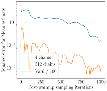
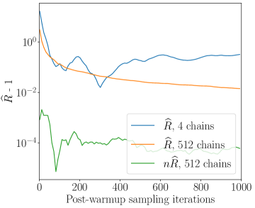
Figure 1: MCMC for $\mathbb{E}(\theta_{1})$ in the Rosenbrock distribution. (left) Squared error of Monte Carlo estimators after warmup. (right) $\widehat{R}$ computed with 4 or 512 chains, and $\mathfrak{n}\widehat{R}$ with 4 groups of 128 subchains.

We first examine the behavior of $\widehat{R}$ in the classic regime and the many-short-chains regime of MCMC. Consider the Rosenbrock distribution $p(\theta_{1},\theta_{2})$,

$$\theta_{1}\sim\text{normal}(0,1)\ ;\ \ \theta_{2}\mid\theta_{1}\sim\text{normal}(0.03(\theta_{1}^{2}-100),1),$$ (1)

and suppose we wish to estimate $\mathbb{E}_{p}(\theta_{1})$, and achieve a squared error below $\text{Var}_{p}(\theta_{1})/100$. This corresponds to the expected squared error attained with 100 independent samples from $p(\theta_{1},\theta_{2})$. We run ChEES-HMC (Hoffman et al., 2021) on a T4 GPU (available for free on Google Colaboratory), first using 4 chains and then using 512 chains. We discard the first 100 iterations as part of the warmup phase and then run 1000 sampling iterations. On a GPU, running ChEES-HMC with 512 chains takes $\sim$20% longer than running 4 chains. Using 4 chains, we require a sampling phase of $\sim$600-700 iterations to achieve our target precision (Figure 1, left). With 512 warmed-up chains, the target error is attained after 1 sampling iteration.

Next we compute the convergence diagnostic $\widehat{R}$, and we check that $\widehat{R}$ is close to 1, for example below the threshold 1.01 proposed by Vehtari et al. (2021). But even after running 1000 sampling iterations, we find that, according to $\widehat{R}$, the sampler has not converged (Figure 1, right), regardless of whether we run 4 chains or 512 chains. Moreover, the computation cost to reduce $\widehat{R}$ to 1.01 far exceeds the cost to achieve our target precision, especially when running many chains. Figure 1 further suggests that this cost does not depend on the number of chains, a conjecture we will verify.

In this paper, we show that for $\widehat{R}$ to go to 1, the variance of the Monte Carlo estimator generated by a single chain must decrease to 0. This criterion cannot be met if each individual chain is short. Crucially, $\widehat{R}$ is a measure of mixing of the chains, which is a separate question than whether the final Monte Carlo estimator, obtained by averaging all the chains, has an acceptable error. For a simple example, consider a large number of chains started at random positions from the target distribution (or, equivalently, warmed up long enough to approximate independent draws from the target). Inference can be fine after a single post-warmup iteration, even though it could take a long time for the chains to mix.

1.2 Main Ideas: nonstationary variance and nested $\widehat{R}$

To address this issue, we introduce nested $\widehat{R}$, denoted $\mathfrak{n}\widehat{R}$. The key idea is to compare clusters of chains or superchains rather than individual chains. In order to still track the influence of the initialization, we require all the chains within a superchain to start at the same location. After a sufficiently long warmup, $\mathfrak{n}\widehat{R}$ decays to 1 with the number of subchains, even when each chain remains short. We show this on our motivating example, where we split the 512 chains into 4 superchains of 128 subchains; see the right panel of Figure 1.

Our approach can be motivated by an analysis of the Monte Carlo estimator’s variance. Consider a state space $\Theta$ over which the target distribution $p$ is defined, and suppose we want to estimate $\mathbb{E}(f(\theta))$, where $\theta\in\Theta$ and $f$ maps $\theta$ to a univariate variable. In practice were are interested in multiple such functions $f$. Let $\bar{f}^{(1)}$ be the Monte Carlo estimator generated by a single Markov chain and let $\Gamma$ be the distribution of $\bar{f}^{(1)}$; that is,

$$\bar{f}^{(1)}\sim\Gamma.$$ (2)

$\Gamma$ is characterized by an initial draw from a starting distribution, $\theta_{0}\sim p_{0}$, and then $\gamma$, the construction of the Markov chain starting at $\theta_{0}$. The process $\gamma$ includes the warmup phase (which is discarded) and the sampling phase. Then by the law of total variance

$$\text{Var}_{\Gamma}\ \bar{f}^{(1)}=\underbrace{\text{Var}_{p_{0}}\left[\mathbb{E}_{\gamma}(\bar{f}^{(1)}\mid\theta_{0})\right]}_{\text{nonstationary variance}}+\underbrace{\mathbb{E}_{p_{0}}\left[\text{Var}_{\gamma}(\bar{f}^{(1)}\mid\theta_{0})\right]}_{\text{persistent variance}}.$$ (3)

We call the first term on the right side of eq. 3 the nonstationary variance and propose to use it as a formal measure of how well the Markov chain forgets its starting point. Indeed, if the warmup phase is sufficiently long, the initialization should only have a negligible influence on $\mathbb{E}(\bar{f}^{(1)})$ and so the nonstationary variance should be close to 0 (even when the sampling phase is short). Furthermore, the nonstationary variance acts as a “proxy clock” for the bias, which also decays as the length of the warmup phase increases. We will illustrate, in an example, that both the squared bias and the nonstationary variance decay at the same rate. It is therefore useful to monitor the nonstationary variance in order to establish whether the warmup phase is sufficiently long for the bias to decay.

The second term on the right side of eq. 3 is the persistent variance: even if the chain reaches stationarity during warmup, the persistent variance remains large and can only decay after a long sampling phase. Therefore, the persistent variance is a nuisance when checking that the Markov chain has (approximately) converged during the warmup phase. Naturally, it is important to check that the persistent variance is small and that the sampling phase is sufficiently long. However we distinguish this from the problem of assessing convergence to the stationary distribution. Following Vehtari et al. (2021), we assess the variance of $\bar{f}^{(1)}$, using the Monte Carlo standard error (MCSE) or the effective sample size (ESS), only once approximate stationarity is established.

Figure 2: Expected squared error for the Monte Carlo estimator generated by a superchain. The estimator is obtained by taking the sample mean of a superchain, after discarding the warmup phase.

To understand the behavior of $\mathfrak{n}\widehat{R}$, we must now analyze the variance of the Monte Carlo estimator returned by a superchain, i.e. a cluster of chains initialized at the same point and then run independently. We show that in this case, the persistent variance decreases linearly with the number of subchains and so becomes small if we run a large number of chains. On the other hand, the nonstationary variance remains unchanged, reflecting the unchanged bias. $\mathfrak{n}\widehat{R}$ can then effectively monitor the nonstationary variance of the Markov chain, even when each individual chain is short, provided we run many chains. Figure 2 summarizes the driving idea behind $\mathfrak{n}\widehat{R}$.

1.3 Outline and contributions

The paper is organized as follows:

• We define $\mathfrak{n}\widehat{R}$ as a generalization of $\widehat{R}$ and analyze the variance of the Monte Carlo estimator produced by a superchain. We showcase $\mathfrak{n}\widehat{R}$’s ability to effectively monitor the nonstationary variance. In the edge case where each Markov chain contains one sample, we propose an exact correction to remove the influence of the persistent variance.

• We then consider a setting where the behavior of $\mathfrak{n}\widehat{R}$ can be analyzed analytically: the continuous time limit of MCMC when targeting a Gaussian distribution, attained by a Langevin diffusion. In this context, we show that the nonstationary variance decays at the same exponential rate as the squared bias.

• We empirically study the variance of $\mathfrak{n}\widehat{R}$ at various phases of the MCMC warmup. Given a fixed total number of chains, we find that no choice of superchain size uniformly minimizes the variance of $\mathfrak{n}\widehat{R}$ and we provide some recommendations. Finally, we showcase the use of $\mathfrak{n}\widehat{R}$ across a range of Bayesian modeling problems, including ones where mixing is slow, the target is multimodal, or the parameter space is moderately high-dimensional ($d=501$).

Throughout the paper, details of proofs are relegated to Appendix A.

2 Nested $\widehat{R}$

The motivation for $\mathfrak{n}\widehat{R}$ is to construct a diagnostic which does not conflate poor convergence and short sampling phase. $\mathfrak{n}\widehat{R}$ works by comparing Monte Carlo estimators whose persistent variance decreases with the number of chains. However, the bias does not decrease with the number of chains and this should be reflected in the nonstationary variance. Our solution is introduce superchains, which are groups of chains initialized at the same point and then run independently.

Consider an MCMC process over a state space $\Theta$ which converges in $D_{\text{TV}}$ to $p$ for any choice of initialization, and denote the starting distribution $p_{0}$. Suppose our goal is to estimate $\mathbb{E}(f(\theta))$ for some function $f$ which maps $\theta$ to a univariate variable and assume furthermore that $\text{Var}_{p}f(\theta)<\infty$.

We generate $K$ superchains, each comprising $M$ subchains initialized at a common point $\theta^{k}_{0}\sim p_{0}$. In the case where each superchain only contains a single subchain, i.e. $M=1$, we recover the classic regime of MCMC. Each subchain is made of $\mathcal{W}$ warmup iterations, which we discard, and $N$ sampling iterations. We denote as $\theta^{(nmk)}$ the $n$th draw from chain $m$ of superchain $k$. The sample mean of each superchain is

$$\bar{f}^{(..k)}=\frac{1}{MN}\sum_{m=1}^{M}\sum_{n=1}^{N}f\left(\theta^{(nmk)}\right).$$ (4)

Moving forward, we write $f^{(nmk)}=f(\theta^{(nmk)})$ to alleviate the notation. The final Monte Carlo estimator is obtained by averaging all the superchains,

$$\bar{f}^{(\cdot\cdot\cdot)}=\frac{1}{K}\sum_{k=1}^{K}\bar{f}^{(\cdot\cdot k)}.$$ (5)

We now define $\mathfrak{n}\widehat{R}$.

Definition 2.1.

Consider the estimator $\mathfrak{n}\widehat{B}$ of the between-superchain variance,

$$\mathfrak{n}\widehat{B}=\frac{1}{K-1}\sum_{k=1}^{K}\left(\bar{f}^{(\cdot\cdot k)}-\bar{f}^{(\cdot\cdot\cdot)}\right)^{2},$$ (6)

and the estimator $\mathfrak{n}\widehat{W}$ of the within-superchain variance,

$$\mathfrak{n}\widehat{W} = \frac{1}{K}\sum_{k=1}^{K}\left(\tilde{B}_{k}+\tilde{W}_{k}\right),$$ (7)

where we require either $N>1$ or $M>1$, and we introduce the estimators $\tilde{B}_{k}$ of the between-chain variance and $\tilde{W}_{k}$ of the within-chain variance, that is

$$\tilde{B}_{k} \triangleq \begin{cases}\frac{1}{M-1}\sum_{m=1}^{M}\left(\bar{f}^{(\cdot mk)}-\bar{f}^{(\cdot\cdot k)}\right)^{2}&\ \text{if \ }M>1,\\ 0&\ \text{if \ }M=1,\end{cases}$$

$$\tilde{W}_{k} \triangleq \begin{cases}\frac{1}{M}\sum_{m=1}^{M}\frac{1}{N-1}\sum_{n=1}^{N}\left(f^{(nmk)}-\bar{f}^{(\cdot mk)}\right)^{2}&\ \text{if \ }N>1,\\ 0&\ \text{if \ }N=1.\end{cases}$$

Then $\mathfrak{n}\widehat{R}$ is the ratio between the total sample standard deviation across all super chains and the average within-superchain sample standard deviation, that is

$$\mathfrak{n}\widehat{R}\triangleq\sqrt{\frac{\mathfrak{n}\widehat{W}+\mathfrak{n}\widehat{B}}{\mathfrak{n}\widehat{W}}}=\sqrt{1+\frac{\mathfrak{n}\widehat{B}}{\mathfrak{n}\widehat{W}}}.$$ (8)

Remark 2.2.

In the edge case where $M=1$, $\mathfrak{n}\widehat{R}$ reduces to $\widehat{R}$.

A common practice to assess convergence of the chains is to check that $\widehat{R}\leq 1+\epsilon$, for some $\epsilon>0$. The choice of $\epsilon$ has evolved over time, starting at $\epsilon=0.1$ (Gelman and Rubin, 1992) and recently using the more conservative value $\epsilon=0.01$ (Vehtari et al., 2021). In the proposed nested design, we now check whether $\mathfrak{n}\widehat{R}\leq 1+\epsilon$ or equivalently,

$$\mathfrak{n}\widehat{B}\leq 2\epsilon\ \mathfrak{n}\widehat{W}+\mathcal{O}(\epsilon^{2}).$$ (9)

This inequality establishes a tolerance value for $\mathfrak{n}\widehat{B}$, scaled by the within-superchain-variance $\mathfrak{n}\widehat{W}$. Moreover, we want to check that despite the distinct initialization and seed, the sample means of each superchain are in good agreement, as measured by $\mathfrak{n}\widehat{B}$.

3 Properties of nested $\widehat{R}$

We now analyze the properties of $\mathfrak{n}\widehat{R}$ theoretically and illustrates its use on several examples.

3.1 Which quantity does $\mathfrak{n}\widehat{R}$ measure?

To answer this question, we consider the asymptotics of $\mathfrak{n}\widehat{R}$ along $K$, the number of superchains. Applying the law of large numbers,

$$\mathfrak{n}\widehat{B}\overset{\text{a.s}}{\underset{K\to\infty}{\longrightarrow}}\mathfrak{n}B\triangleq\text{Var}_{\Gamma}(\bar{f}^{(\cdot\cdot k)}).$$ (10)

Then by the law of total variance,

$$\mathfrak{n}B=\text{Var}_{p_{0}}\left[\mathbb{E}_{\gamma}(\bar{f}^{(\cdot\cdot k)}\mid\theta^{k}_{0})\right]+\mathbb{E}_{p_{0}}\left[\text{Var}_{\gamma}(\bar{f}^{(\cdot\cdot k)}\mid\theta^{k}_{0})\right].$$ (11)

Because the chains are identically distributed and conditionally independent, we have

$$\mathbb{E}_{\gamma}(\bar{f}^{(\cdot\cdot k)}\mid\theta^{k}_{0}) = \mathbb{E}_{\gamma}(\bar{f}^{(\cdot mk)}\mid\theta^{k}_{0})$$ (12)

$$\text{Var}_{\gamma}(\bar{f}^{(\cdot\cdot k)}\mid\theta^{k}_{0}) = \frac{1}{M}\text{Var}_{\gamma}(\bar{f}^{(\cdot mk)}\mid\theta^{k}_{0}).$$ (13)

Plugging these results back into (11), we obtain the following result.

Theorem 3.1.

Consider a superchain initialized at $\theta^{k}_{0}\sim p_{0}$ and made of $M$ chains. Then the variance of the superchain’s sample mean is

$$\mathfrak{n}B=\underbrace{\mathrm{Var}_{p_{0}}\left[\mathbb{E}_{\gamma}(\bar{f}^{(\cdot mk)}\mid\theta^{k}_{0})\right]}_{\text{nonstationary variance}}+\underbrace{\frac{1}{M}\mathbb{E}_{p_{0}}\left[\mathrm{Var}_{\gamma}(\bar{f}^{(\cdot mk)}\mid\theta^{k}_{0})\right]}_{\text{persistent variance}}.$$ (14)

Hence the superchain has the same nonstationary variance as a single chain, but the persistent variance decreases linearly with $M$.

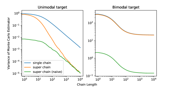
Figure 3: Variance of Monte Carlo estimators, $\bar{f}^{(\cdot\cdot k)}$, constructed using a single chain, a naive superchain of 1024 independent subchains, or a superchain of 1024 subchains initialized at the same point. When the Markov chains converge, the variance of a superchain decreases to the variance of a naive superchain. This transition occurs because the nonstationary variance decays to 0. If the Markov chains do not converge, the variance of a superchain stays large.

We demonstrate this behavior of $\mathfrak{n}B$ on two target distributions: (i) a Gaussian distribution where the chains converge and (ii) a mixture of Gaussians where the chains fail to converge. As benchmarks, we use $B$, the variance of the Monte Carlo estimator generated by a single chain, and $\mathfrak{n}\tilde{B}$, the variance of the Monte Carlo estimator generated by a group of $M$ independent chains with no common initialization. We call such a group a naive superchain. Because there is no initialization constraints, the nonstationary variance of the naive super chain also scales as $1/M$ (but the bias doesn’t!). We run Hamiltonian Monte Carlo (HMC; Neal, 2012; Betancourt, 2018) on a GPU and use $M=1028$ chains for each superchain. Figure 3 shows the results. When the chains converge, $\mathfrak{n}B$ first behaves like $B$ and then transitions to behaving like $\mathfrak{n}\tilde{B}$, as the nonstationary variance decays. On the other hand, when the chains do not converge, the transition does not occur and $\mathfrak{n}B$ stays large.

A first corollary of Theorem 3.1 examines the behavior of $\mathfrak{n}\widehat{R}$ after a long warmup phase, specifically in the limit where the Markov chains have converged to their stationary distribution.

Corollary 3.2.

Suppose that all chains within a superchain start at the same point $\theta_{0}^{k}\sim p_{0}$ and that each chain is made of $M$ subchains. Assume further that $N>1$ and the chains have positive autocorrelation. Then, for an infinitely long warmup phase,

$$\underset{\mathcal{W}\to\infty}{\lim}\sqrt{1+\frac{\mathfrak{n}B}{\mathfrak{n}W}}\geq\sqrt{1+\frac{1}{M}\frac{1-1/N}{\mathrm{ESS}_{(1)}+1/N}},$$ (15)

where $\mathrm{ESS}_{(1)}$ is the effective sample size for a single chain of length $N$.

From the above, we see that without the nesting design (i.e. $M=1$ case), $\widehat{R}$ can only decay to 1 if $\text{ESS}_{(1)}$ is large, because we need to kill off the persistent variance. This explains the results seen in Figure 1 and echoes the observation by Vats and Knudson (2021) that for stationary Markov chains, $\widehat{R}$ (or rather the quantity measured by $\widehat{R}$) is a one-to-one map with the ESS. We emphasize however that this equivalence does not hold when the chains are not stationary and $\mathcal{W}<\infty$.

In general, increasing $M$ and $N$ reduces the persistent variance and so makes $\mathfrak{n}B$ a sharper upper bound on the nonstationary variance. When $N=1$, that is each chain only contains one sampling iteration, we can correct exactly for the contribution of the persistent variance to $\mathfrak{n}\widehat{R}$. The $N=1$ case is mathematically convenient and takes the logic of the many-short-chains regime to its extreme, with the variance reduction entirely handled by the number of chains.

Corollary 3.3.

Suppose that all chains within a superchain start at the same point $\theta_{0}^{k}\sim p_{0}$ and that each chain is made of $M$ subchains. Assume further that $N=1$. Then

$$\sqrt{1+\frac{\mathfrak{n}B}{\mathfrak{n}W}}=\sqrt{1+\frac{1}{M}+\frac{\mathrm{Var}_{p_{0}}\mathbb{E}_{\gamma}(f^{(1mk)}\mid\theta^{k}_{0})}{\mathbb{E}_{p_{0}}\mathrm{Var}_{\gamma}(f^{(1mk)}\mid\theta^{k}_{0})}}.$$ (16)

Above, the persistent variance, scaled by the expected within-chain variance, reduces to exactly $1/M$ and so it is possible to correct for the nuisance term and adjust the threshold for $\mathfrak{n}\widehat{R}$ accordingly. This result does not depend on the transition kernel, nor on the length of the warmup phase, and it applies to nonstationary Markov chains.

3.2 Bias and nonstationary variance

We have established that $\mathfrak{n}\widehat{R}$ monitors the nonstationary variance. Now the primary goal of the warmup phase is to reduce the bias. In this section, we examine the connection between the nonstationary variance and the bias in an illustrative example. We first define the idea of reliability for a convergence diagnostic.

Definition 3.4.

For a univariate random variable $f$, we say an MCMC process is $(\delta,\delta^{\prime})$-reliable for $\mathfrak{n}\widehat{R}$ if

$$\frac{\mathfrak{n}B}{\mathfrak{n}W}\leq\delta\implies\frac{(\mathbb{E}_{\Gamma}\bar{f}^{(\cdot m)}-\mathbb{E}_{p}f)^{2}}{\mathrm{Var}_{p}f}\leq\delta^{\prime}.$$ (17)

Since $\widehat{R}$ is a special case of $\mathfrak{n}\widehat{R}$, we have also defined reliability for $\widehat{R}$. Gelman and Rubin (1992) tackled the question of $\widehat{R}$’s reliability by using an overdispersed initialization. Here, we provide a formal proof that in the Gaussian case $(\delta,\delta^{\prime})$-reliability is equivalent to using an initial distribution $p_{0}$ with a large variance relative to the initial bias. The Gaussian case provides intuition for unimodal targets and can be a reasonable approximation after rank normalization of the samples (Vehtari et al., 2021).

Let $p=\text{normal}(\mu,\sigma)$. To approximate a large class of MCMC processes, we consider the solution $(X_{t})_{t\geq 0}$ of the Langevin diffusion targeting $p$ defined by the stochastic differential equation

$$dX_{t}=-\,(X_{t}-\mu)dt+\sqrt{2\sigma}\,dW_{t},$$ (18)

where $(W_{t})_{t\geq 0}$ is a standard Brownian motion. The convergence of MCMC toward continuous-time stochastic processes has been widely studied, notably by Gelman et al. (1997) and Roberts and Rosenthal (1998), who established scaling limits of random walk Metropolis and the Metropolis adjusted Langevin algorithm toward Langevin diffusion. Similar studies have been conducted for Hamiltonian Monte Carlo and its extensions; see, e.g., Beskos et al. (2013), Riou-Durand and Vogrinc (2022). Typically, the solution of a continuous-time process after a time $T>0$ is approximated by a Markov chain, discretized with a time step $h>0$ and run for $\lfloor T/h\rfloor$ steps. We consider here a Gaussian initial distribution $p_{0}=\text{normal}(\mu_{0},\sigma_{0})$. In this setup, the bias and the variance of the Monte Carlo estimator admit an analytical form.

The solution $X_{T}$ is interpreted as an approximation as $h\rightarrow 0$ of the setting of parallel chains for $\mathcal{W}=\lfloor T/h\rfloor$ iterations and $N=1$, i.e., $\theta^{(1mk)}=X_{T}$. This scenario is the simplest one to analyze and illustrates an edge case of the many-short-chains regime.

The main result of this section states that the squared bias and scaled nonstationary variance decay at a rate $\sim e^{-2T}$, providing justification as to why the latter can be used as a proxy clock for the former.

Theorem 3.5.

Let $(X_{t})_{t\geq 0}$ be the solution of (18) starting from $X_{0}\sim\pi_{0}$. Then for any warmup time $T>0$, the bias is

$$\mathbb{E}\bar{\theta}^{(1\cdot k)}-\mathbb{E}_{\pi}X=\mathbb{E}X_{T}-\mathbb{E}_{\pi}X=(\mu_{0}-\mu)e^{-T}.$$ (19)

Furthermore,

$$\frac{\mathfrak{n}B}{\mathfrak{n}W}=\frac{\mathrm{Var}_{\pi_{0}}\mathbb{E}(X_{T}\mid X_{0})}{\mathbb{E}_{\pi_{0}}\mathrm{Var}(X_{T}\mid X_{0})}=\frac{1}{M}+\frac{\sigma_{0}^{2}}{\sigma^{2}(e^{2T}-1)}.$$ (20)

We end this section with a corollary that states that the initialization needs to be sufficiently dispersed for $\mathfrak{n}\widehat{R}$ to be reliable.

Corollary 3.6.

Let $\delta>0$ and $\delta^{\prime}>0$. Assume the conditions stated in Theorem 3.5. If $(\mu_{0}-\mu)^{2}/\sigma^{2}\leq\delta^{\prime}$, $\mathfrak{n}\widehat{R}$ is trivially $(\delta,\delta^{\prime})$-reliable. If $(\mu_{0}-\mu)^{2}/\sigma^{2}>\delta^{\prime}$, then $\mathfrak{n}\widehat{R}$ is $(\delta,\delta^{\prime})$-reliable if and only if

$$\sigma_{0}^{2}>\left(\delta-\frac{1}{M}\right)\left(\frac{(\mu-\mu_{0})^{2}}{\delta^{\prime}\sigma^{2}}-1\right)\sigma^{2}.$$ (21)

Remark 3.7.

If $\delta<1/M$, $\mathfrak{n}\widehat{R}$ is trivially reliable in the sense that (on average) we never declare convergence, no matter how long $T$ is.

Appendix B provides additional results on the reliability of $\mathfrak{n}\widehat{R}$. In details, we numerically test the lower bound provided by Corollary 3.6 on a Gaussian and a mixture of Gaussians, and we then derive a similar bound for $\widehat{R}$ when $N>1$.

3.3 Variance of $\mathfrak{n}\widehat{R}$

In the previous sections, we focused on the quantity measured by $\mathfrak{n}\widehat{R}$, attained in the limit of a large number of superchains, that is $K\to\infty$. We now assume a finite number of superchains. Even if $\mathfrak{n}\widehat{R}$ is $(\delta,\delta^{\prime})$-reliable, it may be too noisy to be useful. An example of this arises in the multimodal case, where all $K$ superchains may initialize by chance in the attraction basin of the same mode. In this scenario, $K$ is too small and we drastically underestimate $\mathfrak{n}B=\text{Var}_{\Gamma}\bar{f}^{(\cdot\cdot k)}$. One would need enough superchains with distinct initializations to find multiple modes and diagnose the chains’ poor mixing.

When using $\widehat{R}$ it seems reasonable to increase the number of chains as much as possible. The question is more subtle for $\mathfrak{n}\widehat{R}$: given a fixed total number of chains $KM$ how many superchains should we run? In general no choice of $K$, given $KM$, minimizes the variance of $\mathfrak{n}\widehat{B}/\mathfrak{n}\widehat{W}$ across all stages of MCMC.

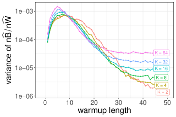
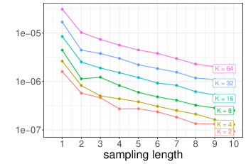
Figure 4: Variance of $\mathfrak{n}\widehat{B}/\mathfrak{n}\widehat{W}$ when running $KM=2048$ chains split into $K$ superchains. (left) $\mathfrak{n}\widehat{B}/\mathfrak{n}\widehat{W}$ is computed using $N=1$ samples after a varying warmup length. No choice of $K$ uniformly minimizes the variance across all phases of MCMC. (right) This time, the chains are stationary. Increasing the length of the sampling phase $N$ reduces the variance of $\mathfrak{n}\widehat{B}/\mathfrak{n}\widehat{W}$.

We demonstrate this phenomenon when targeting a Gaussian with $KM=2048$ chains (Figure 4, left). Here the choice $K=2$ minimizes the variance once the chains are stationary but nearly maximizes it during the early stages of the warmup phase. For $K$ small, all the chains may be in agreement by chance even when they are not close to the stationary distribution. Increasing $K$ helps avoid this scenario. On the other hand, a large $K$ results in a large variance once the chains approach their stationary distribution. This is because the persistent variance remains large if $K$ is large (and therefore $M$ is small), even once the nonstationary variance vanishes. In other words $\mathfrak{n}\widehat{B}$ remains noisy because of a large nuisance term. We now see the competing forces at play when choosing $K$. Empirically, we will find that several choices of $K$ work well across a collection of problems (Section 4).

The variance of $\mathfrak{n}\widehat{R}$ can be further reduced by increasing the length of the sampling phase $N$. The right panel of Figure 4 demonstrates the reduction in variance as $N$ varies from 1 to 10. For many problems, running 10 more iterations is computationally cheap. A large $N$ also makes $\mathfrak{n}B$ a sharper upper bound on the nonstationary variance. However, if $N>1$, we cannot use Corollary 3.3 to exactly characterize and correct for the persistent variance.

3.4 Error tolerance and threshold for $\mathfrak{n}\widehat{R}$

Ultimately, our goal is to control the error of our Monte Carlo estimators. Consider the bias-variance decomposition for an estimator returned by a superchain,

$$\mathbb{E}_{\Gamma}\left((\bar{f}^{(\cdot\cdot k)}\right. \left.-\mathbb{E}_{p}f)^{2}\right)$$

$$=\underbrace{(\mathbb{E}_{\Gamma}\bar{f}^{(\cdot\cdot k)}-\mathbb{E}_{p}f)^{2}}_{\text{squared bias}}+\underbrace{\text{Var}_{p_{0}}(\mathbb{E}_{\gamma}(\bar{f}^{(\cdot\cdot k)}\mid\theta^{k}_{0}))}_{\text{nonstationary variance}}+\underbrace{\mathbb{E}_{p_{0}}(\text{Var}_{\gamma}(\bar{f}^{(\cdot\cdot k)}\mid\theta^{k}_{0}))}_{\text{persistent variance}}.$$ (22)

Much of the MCMC literature focuses on the final term, with the assumption that we have run the Markov chain’s warmup “long enough” for them to be approximately stationary, at which point the bias (and the nonstationary variance) become negligible. The error tolerance can then be expressed in terms of the MCSE and the ESS (e.g. Flegal et al., 2008; Gelman et al., 2013; Vats et al., 2019; Vehtari, 2022). What constitutes an appropriate ESS is problem-dependent and also subject to academic discussion (e.g Mackay, 2003; Gelman and Shirley, 2011; Vats et al., 2019; Vehtari, 2022; Margossian and Gelman, 2023).

If the Markov chains are not close to stationarity, variance alone cannot characterize the expected squared error, and so we must first check for approximate convergence, for instance with $\widehat{R}$ or $\mathfrak{n}\widehat{R}$. Picking a threshold for $\mathfrak{n}\widehat{R}$ morally amounts to setting a tolerance $\tau$ on the scaled nonstationary variance

$$\frac{\text{Var}_{p_{0}}\left(\mathbb{E}_{\gamma}(\bar{f}^{(\cdot\cdot k)}\mid\theta^{k}_{0})\right)}{\mathbb{E}_{p_{0}}\left(\text{Var}_{\gamma}(\bar{f}^{(\cdot\cdot k)}\mid\theta^{k}_{0})\right)}\leq\tau.$$ (23)

Since we measure the total variance rather than the nonstationary variance, we need to correct for the persistent variance by either running more subchains, or falling back on the $N=1$ case to apply Corollary 3.3, which tells us that the scaled persistent variance is exactly $1/M$. We use the latter and construct our threshold as

$$\mathfrak{n}\widehat{R}\leq\sqrt{1+\frac{1}{M}+\tau}.$$ (24)

The choice of $\tau$ itself, just like the tolerable expected squared error, depends on the problem. We propose to make the nonstationary variance—and so, by the proxy clock heuristic, the squared bias—small next to the tolerable squared error. Then the error is dominated by the persistent variance and can be characterized by estimators of the MCSE. We will demonstrate such an approach on a collection of examples.

4 Numerical experiments

Target	$d$	Description
Rosenbrock	2	A joint normal distribution nonlinearly transformed to have
		high curvature (Rosenbrock, 1960). See Equation 1. This
		target produces Markov chains with a large autocorrelation.
Eight Schools	10	The posterior for a hierarchical model of the effect of a test-
		preparation program for high school students (Rubin, 1981).
		Fitting such a model with MCMC requires a careful
		reparameterization (Papaspiliopoulos et al., 2007).
German Credit	25	The posterior of a logistic regression applied to a numerical
		version of the German credit data set (Dua and Graff, 2017).
Pharmacokinetics	45	The posterior for a hierarchical model describing the absorption
		of a drug compound in patients during a clinical trial
		(e.g Wakefield, 1996; Margossian et al., 2022), using data
		simulated over 20 patients. This model uses a likelihood based
		on an ordinary differential equation.
Bimodal	100	An unbalanced mixture of two well-separated Gaussians. With
		standard MCMC, each Markov chain “commits” to a single mode,
		leading to bias sampling. Even after a long compute time, the
		Markov chains fail to converge.
Item Response	501	The posterior for a model to assess students’ ability based on
		test scores (Gelman and Hill, 2007). The model is fitted to the
		response of 400 students to 100 questions, and the model
		estimates (i) the difficulty of each question and (ii) each student’s.
		aptitude. This problem has a relatively high dimension.

Table 1: Target distributions for our numerical experiments.

We demonstrate an MCMC workflow using $\mathfrak{n}\widehat{R}$ on a diversity of applications mostly drawn from the Bayesian literature. Our focus is on producing accurate estimates for the first moment for the model parameters. We consider six targets which represent a diversity of applications, notably in Bayesian modeling. Table 1 summarises the target distributions with more details available in Appendix C. The bimodal example provides a case where the chains fail to converge after a reasonnable amount of compute time. As our MCMC algorithm, we run ChEES-HMC (Hoffman et al., 2021), which is an adaptive HMC sampler (Neal, 2012; Betancourt, 2018). The algorithm is implemented in TensorFlow Probability (TensorFlow Probability Development Team, 2023).

4.1 Monte Carlo squared error after convergence

We construct a model of the squared error for stationary Markov chains, and use this as a benchmark for the empirical squared error. In the stationarity limit, i.e. $\mathcal{W}\to\infty$, the subchains within a superchain are no longer correlated. A central limit theorem may then be taken along the total number of chains. Then for $N=1$, the scaled squared error approximatively follows a $\chi^{2}$ distribution,

$$E^{2}\triangleq\frac{KM}{\text{Var}_{p}f}(\bar{f}^{(1\cdot\cdot)}-\mathbb{E}_{p}f)^{2}\overset{\text{approx.}}{\sim}\chi^{2}_{1}.$$ (25)

High-precision estimates of $\mathbb{E}_{p}f$ and $\text{Var}_{p}f$ are computed using long MCMC runs (Appendix C). We use the above approximation to jointly model the expected squared error at stationarity across all dimensions. This is somewhat of a simplification, since we do not account for the correlations between dimensions.

After a sufficiently long warmup phase, the Markov chains are nearly stationary and $E^{2}$ approximately follows a $\chi^{2}_{1}$ distribution. This should ideally be reflected by $\mathfrak{n}\widehat{R}\approx 1$. However if the warmup phase is too short and the squared error large because of the Markov chain’s bias, we expect to see $\mathfrak{n}\widehat{R}\gg 1$, per the proxy clock heuristic.

4.2 Results when running 2048 chains with $K=16$ superchains

Suppose we target an ESS of $\sim$2000. In this case, we may run 2048 chains, broken into $K=16$ superchains and $M=128$ subchains. For each target distribution, we compute $\mathfrak{n}\widehat{R}$ using $N=1$ draw after warmups of varying lengths,

$$\ell=(10,20,30,\dots,100,200,300,\dots,1000).$$

$\ell$ contains both warmup lengths that are clearly too short to achieve convergence and lengths after which approximate convergence is expected when running HMC. That way, the behavior of $\mathfrak{n}\widehat{R}$ can be examined on both nonstationary and (nearly) stationary Markov chains. At the end of each warmup window, we record $\mathfrak{n}\widehat{R}$ for each dimension and the corresponding $E^{2}$ using a single draw per chain. We repeat our experiment 10 times for each model.

Figure 5 plots $E^{2}$ against $\mathfrak{n}\widehat{R}$. For all targets, we observe a correlation between $\mathfrak{n}\widehat{R}$ and $E^{2}$. After a short warmup, the chains are far from their stationary distribution: this manifests as both a large $E^{2}$ and a large $\mathfrak{n}\widehat{R}$. When $\mathfrak{n}\widehat{R}$ is close to 1, the squared error is smaller and approaches the distribution we would expect from stationary Markov chains (Section 4.1). For the bimodal target, the Markov chains fail to converge after a warmup of 1000 iterations and our experiment only reports observations where $E^{2}$ and $\mathfrak{n}\widehat{R}$ are both large.

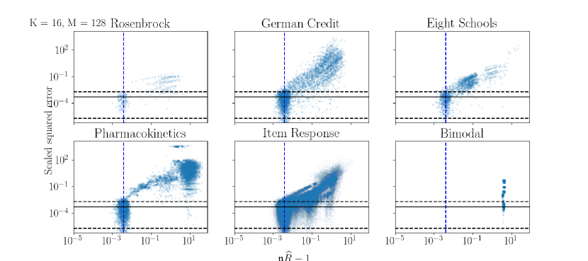
Figure 5: Scaled squared error against $\mathfrak{n}\widehat{R}$, using $K=16$, $M=128$ and $N=1$. For short warmup phases, the Markov chains are far from their stationary distribution, which manifests as a large squared error and a large $\mathfrak{n}\widehat{R}$. Once $\mathfrak{n}\widehat{R}$ is close to 1, the scaled squared error behaves as we would expect from stationary Markov chains (Section 4.1). The vertical blue line corresponds to the proposed threshold $\epsilon\approx 0.004$. The horizontal lines show the median (solid line) and 0.9 coverage (dashed lines) for the squared error of a stationary Markov chain.

As a tolerance on the scaled nonstationary variance, we consider $\tau=10^{-4}$, which corresponds to a fifth of the scaled variance we tolerate with an ESS of 2000. The tolerance for $\mathfrak{n}\widehat{R}$ is then $\sim$1.004, which is smaller than the recommended threshold of 1.01 for $\widehat{R}$. Bear in mind the tolerance we chose is relative to our target ESS, which can change between problems. Figure 6 plots the fraction of times the scaled squared error is above the $0.95^{\text{th}}$ quantile of a $\chi^{2}_{1}$ distribution for $\mathfrak{n}\widehat{R}$ below varying thresholds. For $\mathfrak{n}\widehat{R}\leq\sqrt{1+1/M+\tau}$, this fraction approaches 0.05 for all models but can be larger.

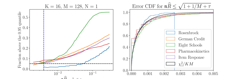
Figure 6: (left) Fraction of Monte Carlo estimates with squared error above the $95^{\text{th}}$ quantile of the stationary error distribution (Section 4.1). The vertical blue line is the prescribed threshold $\sqrt{1+1/M+\tau}$. (right) For $\mathfrak{n}\widehat{R}$ close to 1, the empirical CDF approaches the theoretical CDF for stationary Markov chains.

4.3 Results when varying the number of superchains $K$

Next we keep the total number of chains fixed and vary $K$. Figure 7 plots the results. The threshold for $\mathfrak{n}\widehat{R}$ is adjusted as $M$ varies, although the tolerance on the nonstationary variance $\tau$ remains unchanged. For $K\in\{8,16,64,256\}$ we find that the $95^{\text{th}}$ quantile of $E^{2}$ is in reasonable agreement with the 95${}^{\text{th}}$ quantile of a $\chi^{2}_{1}$, albeit slightly larger. The results are less stable for the extreme choices $K=2$ and $K=1024$. For $K=2$ we expect the variance of $\mathfrak{n}\widehat{R}$ to be large during the early stages of MCMC, while for $K=1024$, the variance is high near stationarity (Section 3.3). Overall, there is a broad range of choices for $K$ away from these extremes that yield a functioning convergence diagnostic in the considered examples.

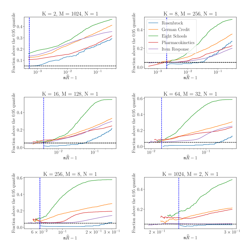
Figure 7: Fraction of Monte Carlo estimates with squared error above the 95th quantile of the stationary error distribution (Section 4.1) when varying $K$. For $K$ between 8 and 256, the fraction approaches the expected 0.05 (horizontal dotted line) for stationary Markov chains, past the prescribed threshold (vertical blue line).

5 Discussion

While CPU clock speeds stagnate, parallel computational resources continue to get cheaper. The question of how to make effective use of these parallel resources for MCMC remains an outstanding challenge. This paper tackles the problem of assessing approximate convergence. We propose a new convergence diagnostic, $\mathfrak{n}\widehat{R}$, which is straightforward to implement for a broad class of MCMC algorithms and works for both long and short chains, in the sense that $\widehat{R}$ works for long chains. A small $\mathfrak{n}\widehat{R}$ (or $\widehat{R}$) does not guarantee convergence to the stationary distribution or that the bias has decayed to 0. Still $\widehat{R}$ has empirically proven its usefulness in applied statistics, machine learning, and many scientific disciplines. Our analysis reveals that potential success (or failure) of $\mathfrak{n}\widehat{R}$ and $\widehat{R}$ is best understood by studying (i) the relation between the nonstationary variance and the squared bias, and (ii) how well $\mathfrak{n}\widehat{R}$ monitors the nonstationary variance.

In addition to working in the many-short-chains regime, $\mathfrak{n}\widehat{R}$ provides more guidance to choose a threshold, notably in the $N=1$ case (Corollary 3.3). Unlike $\widehat{R}$, the proposed $\mathfrak{n}\widehat{R}$ requires a partition of the chains into superchains. No choice of partition uniformly minimizes the variance of $\mathfrak{n}\widehat{R}$ during all phases of MCMC. Based on our numerical experiments, we recommend using $K=8-256$ initializations, when running $KM=2048$ chains.

5.1 Related work

There has recently been a renewed interest in $\widehat{R}$ and its practical implementation (Vehtari et al., 2021; Vats and Knudson, 2021; Moins et al., 2023), with an emphasis on the classical regime of MCMC with 8 chains or fewer. $\widehat{R}$ computes a ratio of two standard deviations and is straightforward to evaluate. However, when applied to samples which are neither independent nor identically distributed—as is the case for MCMC—it becomes difficult to understand which quantity $\widehat{R}$ measures. It is moreover unclear how to choose a threshold for $\widehat{R}$ to decide if the Markov chains have converged. These issues were recently raised by Vats and Knudson (2021) and Moins et al. (2023), who studied the convergence of $\widehat{R}$ in the limit of infinitely long chains. But such an asymptotic analysis tacitly applies to stationary Markov chains and convergence of the Monte Carlo estimator itself during the sampling phase, rather than convergence in $D_{\text{TV}}$ or in bias during the warmup. As prescribed by the many-short-chains regime, we took limits in another direction: an infinite number of finite nonstationary Markov chains. This perspective elicits the nonstationary variance, sheds light on the advantages and limitations of $\widehat{R}$, and motivates $\mathfrak{n}\widehat{R}$.

Beyond running a long warmup phase, many strategies have been proposed to control the bias of Monte Carlo estimators. Examples include annealed importance sampling (Neal, 2001) and sequential Monte Carlo (Del Moral et al., 2006). More recently, unbiased MCMC has been proposed as a paradigm to construct unbiased estimators (Glynn and Rhee, 2014; Jacob et al., 2020). This strategy relies on transition kernels which allow pairs of Markov chains to couple after a finite time. Once a coupling occurs, we can construct unbiased estimators of expectation values. In this sense, the coupling time replaces the traditional warmup phase. Designing such transition kernels with short coupling times is an active area of research (Heng and Jacob, 2019; Jacob et al., 2020; Nguyen et al., 2022), but at present it is not always possible to find a kernel that couples quickly. For example, Hamiltonian Monte Carlo (HMC; Neal, 2012; Betancourt, 2018) methods using many integration steps per proposal are often the only viable option for sampling from poorly conditioned high-dimensional posteriors over a continuous space. Unfortunately the coupling HMC kernel of Heng and Jacob (2019) only couples quickly if the problem is sufficiently well conditioned that HMC converges rapidly with a relatively small number of integration steps per proposal.

Stein methods—see South et al. (2021) and references theirein—, such as Stein thinning (Riabiz et al., 2022), can remove strongly biased samples produced during the early stages of MCMC, and in some sense automatically discard a warmup phase. However, Stein methods can be computationally expensive and may not scale well in high dimensions. Furthermore, if the total length of the Markov chain is too short, no thinning can remove the bias incurred by the initialization—a problem which, arguably, $\mathfrak{n}\widehat{R}$ can detect and so the proposed diagnostic may be used conjointly with Stein methods.

5.2 Future directions

The nesting design we introduce opens the prospect of generalizing other variations on $\widehat{R}$, including multivariate $\widehat{R}$ (Brooks and Gelman, 1998; Vats and Knudson, 2021; Moins et al., 2023), rank-normalized $\widehat{R}$ (Vehtari et al., 2021) and local $\widehat{R}$ (Moins et al., 2023). Nesting can further be used for less conventional convergence diagnostics, such as $R^{*}$, which uses classification trees to compare different chains (Lambert and Vehtari, 2022).

A direction for future work is to adaptively set the warmup length using $\mathfrak{n}\widehat{R}$. This would follow a long tradition of using diagnostics to do early stopping of MCMC (Geweke, 1992; Cowles and Carlin, 1996; Cowles et al., 1998; Jones et al., 2006; Zhang et al., 2020). Still, standard practice remains to prespecify the warmup length. This means the warmup length is rarely optimal, which is that much more exasperating in the many-short-chains regime, where the warmup dominates the computation.

6 Acknowledgments

We thank the TensorFlow Probability team at Google, especially Alexey Radul. We also thank Marylou Gabrié and Sam Livingstone for helpful discussions; Rif A. Saurous, Andrew Davison, Owen Ward, Mitzi Morris, and Lawrence Saul for helpful comments on the manuscript; and the U.S. Office of Naval Research and Research Council of Finland for partial support. LRD was supported by the EPSRC grant EP/R034710/1. Much of this work was done while CM was at Google Research and in the Department of Statistics at Columbia University, and while LRD was in the Department of Statistics at the University of Warwick.

Appendix

Appendix A Proofs

Here we provide the proofs for formal statements throughout the paper.

A.1 Proofs for Section 2: “Nested $\widehat{R}$”

A.1.1 Proof of Corollary 3.2: stationary lower bound for $\mathfrak{n}\widehat{R}$

We first state a lemma giving the asymptotic behavior of $\mathfrak{n}\widehat{W}$ as the number of superchains $K$ goes to infinity.

Lemma A.1.

In the limit of an infinite number of superchains,

$$\lim_{K\to\infty}\mathfrak{n}\widehat{W}=\mathfrak{n}W\triangleq\mathbb{E}_{p_{0}}\text{Var}_{\gamma}(\bar{f}^{(\cdot mk)}\mid\theta^{k}_{0})+W^{\prime},$$ (26)

where

$$W^{\prime}\triangleq\begin{cases}\frac{1}{N-1}\sum_{n=1}^{N}\text{Var}_{\Gamma}f^{(nmk)}-\text{Var}_{\Gamma}\bar{f}^{(\cdot mk)}+(\mathbb{E}_{\Gamma}f^{(nmk)})^{2}-(\mathbb{E}_{\Gamma}f^{(\cdot mk)})^{2}&\ \text{if}\ N>1\\ 0&\ \text{if}\ N=1,\end{cases}$$

Proof.

Recall the superchains are independent. Then applying the law of large numbers along $K$ yields,

$$\mathfrak{n}\widehat{W}\ \xrightarrow[K\to\infty]{a.s}\ \mathbb{E}_{\Gamma}\tilde{B}_{k}+\mathbb{E}_{\Gamma}\tilde{W}_{k}.$$

Now

$$\mathbb{E}_{\Gamma}\tilde{B}_{k} = \frac{1}{M-1}\sum_{m=1}^{M}\mathbb{E}_{\Gamma}\left(\bar{f}^{(\cdot mk)}-\bar{f}^{(\cdot\cdot k)}\right)^{2}$$

$$= \frac{1}{M-1}\sum_{m=1}^{M}\left(\mathbb{E}_{\Gamma}[\bar{f}^{(\cdot mk)}]^{2}+\mathbb{E}_{\Gamma}[\bar{f}^{(\cdot\cdot k)}]^{2}-2\mathbb{E}_{\Gamma}(\bar{f}^{(\cdot mk)}\bar{f}^{(\cdot\cdot k)})\right),$$

and

$$\sum_{m=1}^{M}\mathbb{E}_{\Gamma}(\bar{f}^{(\cdot mk)}\bar{f}^{(\cdot\cdot k)}) = M\frac{1}{M}\sum_{m=1}^{M}\mathbb{E}_{\Gamma}(\bar{f}^{(\cdot mk)}\bar{f}^{(\cdot\cdot k)})$$

$$= M\mathbb{E}_{\Gamma}\left(\frac{1}{M}\sum_{m=1}^{M}\bar{f}^{(\cdot mk)}\bar{f}^{(\cdot\cdot k)}\right)$$

$$= M\mathbb{E}_{\Gamma}[\bar{f}^{(\cdot\cdot k)}]^{2}.$$

Plugging this back in yields,

$$\mathbb{E}_{\Gamma}\tilde{B}_{k} = \frac{1}{M-1}\sum_{m=1}^{M}\left(\mathbb{E}_{\Gamma}[\bar{f}^{(\cdot mk)}]^{2}-\mathbb{E}_{\Gamma}[\bar{f}^{(\cdot\cdot k)}]^{2}\right)$$

$$= \frac{1}{M-1}\sum_{m=1}^{N}\left(\text{Var}_{\Gamma}\bar{f}^{(\cdot mk)}+[\mathbb{E}_{\Gamma}\bar{f}^{(\cdot mk)}]^{2}-\text{Var}_{\Gamma}\bar{f}^{(\cdot\cdot k)}-[\mathbb{E}_{\Gamma}\bar{f}^{(\cdot\cdot k)}]^{2}\right)$$

$$= \frac{1}{M-1}\sum_{m=1}^{N}\left[\text{Var}_{\Gamma}\bar{f}^{(\cdot mk)}-\text{Var}_{\Gamma}\bar{f}^{(\cdot\cdot k)}\right]+\left[(\mathbb{E}_{\Gamma}\bar{f}^{(\cdot mk)})^{2}-(\mathbb{E}_{\Gamma}\bar{f}^{(\cdot\cdot k)})^{2}\right].$$

The second term vanishes, because $\mathbb{E}_{\Gamma}\bar{f}^{(\cdot mk)}=\mathbb{E}_{\Gamma}\bar{f}^{(\cdot\cdot k)}$. Then

$$\mathbb{E}\tilde{B}_{k} = \frac{1}{M-1}\sum_{m=1}^{M}\text{Var}_{\Gamma}\bar{f}^{(\cdot mk)}-\text{Var}_{\Gamma}\bar{f}^{(\cdot\cdot k)}$$

$$= \frac{M}{M-1}\left(\text{Var}_{\Gamma}\bar{f}^{(\cdot mk)}-\text{Var}_{\Gamma}\bar{f}^{(\cdot\cdot k)}\right),$$

We next apply the law of total variance:

$$\text{Var}_{\Gamma}\bar{f}^{(\cdot mk)} = \mathbb{E}_{p_{0}}\text{Var}_{\gamma}(\bar{f}^{(\cdot mk)}\mid\theta^{k}_{0})+\text{Var}_{p_{0}}\mathbb{E}_{\gamma}(\bar{f}^{(\cdot mk)}\mid\theta^{k}_{0}),$$

and

$$\text{Var}_{\Gamma}\bar{f}^{(\cdot\cdot k)} = \mathbb{E}_{p_{0}}\text{Var}_{\gamma}(\bar{f}^{(\cdot\cdot k)}\mid\theta^{k}_{0})+\text{Var}_{p_{0}}\mathbb{E}_{\gamma}(\bar{f}^{(\cdot\cdot k)}\mid\theta^{k}_{0})$$

$$= \frac{1}{M}\mathbb{E}_{p_{0}}\text{Var}_{\gamma}(\bar{f}^{(\cdot mk)}\mid\theta^{k}_{0})+\text{Var}_{p_{0}}\mathbb{E}_{\gamma}(\bar{f}^{(\cdot mk)}\mid\theta^{k}_{0}),$$

where the second line follows from noting that, conditional on $\theta_{0}^{k}$, the chains are independent, and that $\mathbb{E}_{\gamma}(\bar{f}^{(\cdot\cdot k)}\mid\theta^{k}_{0})=\mathbb{E}_{\gamma}(\bar{f}^{(\cdot mk)}\mid\theta^{k}_{0})$. Plugging this result back, we get

$$\mathbb{E}\tilde{B}_{k} = \frac{M}{M-1}\left[\mathbb{E}_{p_{0}}\text{Var}_{\gamma}(\bar{f}^{(\cdot mk)}\mid\theta^{k}_{0})-\frac{1}{M}\mathbb{E}_{p_{0}}\text{Var}_{\gamma}(\bar{f}^{(\cdot mk)}\mid\theta^{k}_{0})\right]$$

$$= \mathbb{E}_{p_{0}}\text{Var}_{\gamma}(\bar{f}^{(\cdot mk)}\mid\theta^{k}_{0}).$$

Next, if $N=1$, $\tilde{W}=0$. If $N>1$, we obtain, following a similar approach as above,

$$\tilde{W}_{k} = \frac{1}{M}\sum_{m=1}^{M}\frac{1}{N-1}\sum_{n=1}^{N}\left(f^{(nmk)}-\bar{f}^{(\cdot mk)}\right)^{2}$$

$$= \frac{1}{M}\sum_{m=1}^{M}\frac{1}{N-1}\sum_{n=1}^{N}\left(f^{(nmk)}\right)^{2}-\left(\bar{f}^{(\cdot mk)}\right)^{2}.$$

Then, taking expectations and expanding the square inside the expectation,

$$\mathbb{E}_{\Gamma}\tilde{W}_{k}=\begin{cases}\frac{1}{N-1}\sum_{n=1}^{N}\text{Var}_{\Gamma}f^{(nmk)}-\text{Var}_{\Gamma}\bar{f}^{(\cdot mk)}+(\mathbb{E}_{\Gamma}f^{(nmk)})^{2}-(\mathbb{E}_{\Gamma}f^{(\cdot mk)})^{2}&\ \text{if}\ N>1\\ 0&\ \text{if}\ N=1,\end{cases}$$ (27)

with the right side corresponding to our definition of $W^{\prime}$. Thus

$$\mathfrak{n}W=\mathbb{E}_{p_{0}}\text{Var}_{\gamma}(\bar{f}^{(\cdot mk)}\mid\theta^{k}_{0})+W^{\prime},$$

as desired. ∎

Remark A.2.

The second term on the right side of eq. 27 is a drift term: the (expected) sample variance increases because the samples do not have the same mean.

We now prove Theorem 3.2.

Proof.

For $\mathcal{W}\to\infty$, the chains are stationary and have “forgotten” their initialization, that is $\text{Var}_{p_{0}}\mathbb{E}_{\gamma}(\bar{f}^{(\cdot mk)}\mid\theta^{k}_{0})=0$. Thus

$$\mathbb{E}_{\Gamma}\tilde{B}_{k}=\mathbb{E}_{p_{0}}\text{Var}_{\gamma}(\bar{f}^{(\cdot mk)}\mid\theta^{k}_{0})=\text{Var}_{\Gamma}\bar{f}^{(\cdot mk)}.$$

Also, because the samples are now all identically distributed, the drift term in $\mathbb{E}_{\Gamma}\tilde{W}$ goes to 0. We also have for any $n$ that $\text{Var}f^{(nmk)}=\sigma^{2}$, where the constant $\sigma^{2}$ is the variance of the stationary distribution, $p$. Furthermore, due the chain’s positive autocorrelation,

$$\text{Var}_{\Gamma}\bar{f}^{(\cdot mk)}\geq\frac{\sigma^{2}}{N}.$$ (28)

Thus

$$\mathfrak{n}W\leq\frac{1}{N-1}\text{Var}_{\Gamma}\bar{f}^{(\cdot mk)}+\frac{N}{N-1}\sigma^{2}.$$

Then

$$\frac{\mathfrak{n}B}{\mathfrak{n}W}\geq\frac{\text{Var}_{\Gamma}\bar{\theta}^{(\cdot mk)}}{M\left(\frac{1}{N-1}\text{Var}_{\Gamma}\bar{\theta}^{(\cdot mk)}+\frac{N}{N-1}\sigma^{2}\right)}.$$

Noting that for stationary chains $\text{ESS}_{(1)}=\sigma^{2}/\text{Var}_{\Gamma}\bar{\theta}^{(\cdot mk)}$,

$$\frac{\mathfrak{n}B}{\mathfrak{n}W}\geq\frac{1}{M\left(\frac{1+N\mathrm{ESS}_{(1)}}{N-1}\right)}==\frac{1}{M}\frac{1-1/N}{\text{ESS}_{(1)}+1/N}.$$

∎

A.1.2 Proof of Corollary 3.3: correction for persistent variance when $N=1$

The proof of Corollary 3.3 follows from Theorem 3.1 and Lemma A.1.

Proof.

When $N=1$, $\tilde{W}_{k}=0$. Thus $\mathfrak{n}W=\mathbb{E}_{p_{0}}\text{Var}_{\gamma}(\bar{f}^{(\cdot mk)}\mid\theta^{k}_{0})$ and

$$\frac{\mathfrak{n}B}{\mathfrak{n}W} = \frac{\mathbb{E}_{p_{0}}\text{Var}_{\gamma}(\bar{f}^{(\cdot mk)}\mid\theta^{k}_{0})}{M\mathbb{E}_{p_{0}}\text{Var}_{\gamma}(\bar{f}^{(\cdot mk)}\mid\theta^{k}_{0})}+\frac{\text{Var}_{p_{0}}\mathbb{E}_{\gamma}(\bar{f}^{(\cdot mk)}\mid\theta^{k}_{0})}{\mathbb{E}_{p_{0}}\text{Var}_{\gamma}(\bar{f}^{(\cdot mk)}\mid\theta^{k}_{0})}$$

$$= \frac{1}{M}+\frac{\text{Var}_{p_{0}}\mathbb{E}_{\gamma}(\bar{f}^{(\cdot mk)}\mid\theta^{k}_{0})}{\mathbb{E}_{p_{0}}\text{Var}_{\gamma}(\bar{f}^{(\cdot mk)}\mid\theta^{k}_{0})}.$$

Finally, $\bar{f}^{(\cdot mk)}=f^{(1mk)}$, given that $N=1$. ∎

A.1.3 Proof of Theorem 3.5: bias and $\mathfrak{n}B/\mathfrak{n}W$ in continuous limit

We prove Theorem 3.5 which gives us an exact expression for the bias and the ratio $\mathfrak{n}B/\mathfrak{n}W$ when using $\bar{X}_{T}$ as our Monte Carlo estimator. Here $\bar{X}_{T}$ is the average of $M$ diffusion processes evaluated at time $T$. The processes are initialized at the same point $X_{0}\sim\pi_{0}$ but then run independently, according to the Langevin diffusion process targeting $\pi=\text{normal}(\mu,\sigma^{2})$.

Proof.

Let $\Psi$ denote the stochastic process which generates $X_{T}$, and further break this process into (i) $\pi_{0}$, the process which draws $x_{0}$ and (ii) $\psi$ the process which generates $X_{T}$ conditional on $x_{0}$. Following the same arguments as in the previous sections of the Appendix, we leverage Corollary 3.3,

$$\frac{\mathfrak{n}B}{\mathfrak{n}W}=\frac{1}{M}+\frac{\mathrm{Var}_{\pi_{0}}\mathbb{E}_{\psi}(X_{T}\mid X_{0})}{\mathbb{E}_{\pi_{0}}\mathrm{Var}_{\psi}(X_{T}\mid X_{0})}.$$

It is well known that Ornstein-Uhlenbeck SDEs, such as the Langevin diffusion SDE targeting a Gaussian, admit explicit solutions; see Gardiner (2004). The solution of eq. 18 given $X_{0}=x_{0}$ is given for $T>0$ by

$$X_{T}=e^{-T}x_{0}+\mu(1-e^{-T})+\sqrt{2\sigma}\int_{0}^{T}e^{-(T-s)}\mathrm{d}W_{s}.$$ (29)

Now, integrating with respect to $X_{0}\sim\pi_{0}=\text{normal}(\mu_{0},\sigma_{0})$ yields

$$\mathbb{E}_{\pi_{0}}\mathbb{E}_{\psi}(X_{T}\mid X_{0})=\mu_{0}e^{-T}+\mu(1-e^{-T}),$$

then

$$\mathrm{Var}_{\pi_{0}}\mathbb{E}_{\psi}(X_{T}\mid X_{0})=\mathrm{Var}_{\pi_{0}}\left(X_{0}e^{-T}+\mu(1-e^{-T})\right)=e^{-2T}\sigma_{0}^{2},$$

and

$$\mathbb{E}_{\pi_{0}}\mathrm{Var}_{\psi}(X_{T}\mid X_{0})\\ =\mathbb{E}_{\pi_{0}}\sigma^{2}(1-e^{-2T})=\sigma^{2}(1-e^{-2T}),$$

from which the desired result follows. ∎

A.1.4 Proof of Corrollary 3.6: initialization conditions under which $\mathfrak{n}\widehat{R}$ is reliable

Theorem 3.6 provides conditions in the continuous limit under which $\mathfrak{n}\widehat{R}$ is $(\delta,\delta^{\prime})$-reliable and formalizes the notion of overdispersed intializations.

Proof.

The bias is given by

$$\mathbb{E}(X_{T})-\mathbb{E}_{\pi}(\mu)=(\mu_{0}-\mu)e^{-T},$$

which is a monotone decreasing function of $T$. The time at which the scaled squared bias is below $\delta^{\prime}$ is obtained by solving

$$\frac{(\mu_{0}-\mu)^{2}e^{-2T}}{\sigma^{2}}\leq\delta^{\prime}.$$

If $(\mu_{0}-\mu)^{2}/\sigma^{2}\leq\delta^{\prime}$, than the above condition is verified for any $T$ and $\mathfrak{n}\widehat{R}$ is trivially $(\delta,\delta^{\prime})$-reliable. Suppose now that $(\mu_{0}-\mu)^{2}/\sigma^{2}>\delta^{\prime}$. Then we require

$$T\geq\frac{1}{2}\log\left(\frac{(\mu_{0}-\mu)^{2}}{\delta^{\prime}\sigma^{2}}\right)\triangleq T^{*}.$$

It remains to ensure that for $T<T^{*}$, $\mathfrak{n}B/\mathfrak{n}W>\delta$. Plugging in $T^{*}$ in the expression from Lemma 3.5 and noting $\mathfrak{n}B/\mathfrak{n}W$ is monotone decreasing in $T$, we have

$$\sigma^{2}_{0}>\left(\delta-\frac{1}{M}\right)\left(e^{2T^{*}}-1\right)\sigma^{2},$$

which is the wanted expression. ∎

Remark A.3.

If $\delta<1/M$, then the condition $\mathfrak{n}B/\mathfrak{n}W<\delta$ cannot be verified. Hence $\mathfrak{n}\widehat{R}$ is reliable in a trivial sense: we never erroneously claim convergence because we never claim convergence.

Appendix B Additional results on the reliability of $\mathfrak{n}\widehat{R}$ and $\widehat{R}$

This appendix provides additional results on the reliability of $\mathfrak{n}\widehat{R}$ (Section 3.2). We numerically test the lower bound on the initial variance, provided by Corollary 3.6, on a Gaussian target and a mixture of two Gaussians. We then derive a reliability condition for $\widehat{R}$, tackling the $N>1$ case where we have more than one sample per chain.

B.1 Numerical evaluation of the reliability of $\mathfrak{n}\widehat{R}$

We numerically evaluate the $(\delta,\delta^{\prime})$-reliability of $\mathfrak{n}\widehat{R}$ on two examples:

• (i) a standard Gaussian, which conforms to the assumption of our theoretical analysis.

• (ii) a mixture of two Gaussians, which constitutes a canonical example where $\widehat{R}$ potentially fails. In this example the Markov chains fail to mix, hence reliability is achieved if $\mathfrak{n}\widehat{R}\geq\sqrt{1+\delta}$.

We approximate the Langevin diffusion using the Metropolis adjusted Langevin algorithm (MALA) algorithm, which is equivalent to HMC with a one-step leapfrog integrator. The step size is 0.04, which is chosen to be as small as possible while ensuring that $\mathfrak{n}\widehat{R}$ reports convergence after $\sim$$2\times 10^{4}$ iterations for the standard Gaussian target. We set $M=16$, $\delta\approx 0.1$ and $\delta^{\prime}=\delta/5$. Reliability is defined in terms of $\mathfrak{n}B$ and $\mathfrak{n}W$, which are the asymptotic limits of $\mathfrak{n}\widehat{B}$ and $\mathfrak{n}\widehat{W}$ when $K\to\infty$. We approximate this limit by using $K=1024$ superchains for a total of 16384 chains.

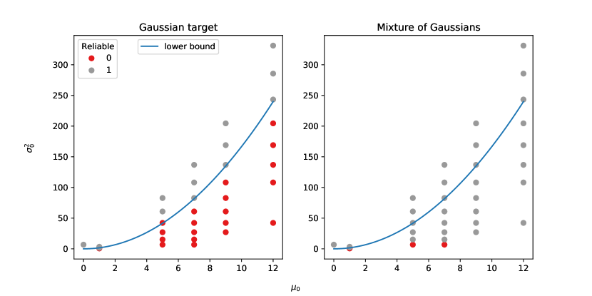
Figure 8: $(\delta,\delta^{\prime})$-reliability of $\mathfrak{n}\widehat{R}$ for varying initial bias $\mu_{0}$ and initial variance $\sigma_{0}^{2}$.

The results are shown in Figure 8. The theoretical lower bound (Theorem 3.6) is accurate when using a standard Gaussian target. When targeting a mixture of Gaussians, the lower bound is too conservative and $\mathfrak{n}\widehat{R}$ is reliable even when using an “underdispersed” initialization. This is because we use a large number of distinct initializations and, even with a small initial variance, we typically find both modes and identify poor mixing. This suggests the failure of $\widehat{R}$ on multimodal targets is often due to using too few distinct initializations, rather than an underdispersed initialization.

B.2 Reliability condition for $\widehat{R}$ in the continuous limit

We here conduct an analysis for $\widehat{R}$ similar to the one conducted for $\mathfrak{n}\widehat{R}$ in Section 3.2. That is we examine the reliability of $\widehat{R}$ when approximating the MCMC chain by a Langevin diffusion which targets a Gaussian.

There are three differences when compared to our study of $\mathfrak{n}\widehat{R}$: (i) each Monte Carlo estimator is now made up of only one chain and all chains are independent, (ii) the chains do not include warmup, i.e., $\mathcal{W}=0$, and (iii) the length of each chain is chosen as $N=\lfloor T/h\rfloor$ for a small value step size $h$ such that for each chain $m$, the distribution of $\theta^{(\lfloor t/h\rfloor m)}$ can be approximated by the Langevin solution defined in (29). The distribution of each (within chain) estimator can therefore be approximated by the distribution of

$$\overline{X}_{T}=\frac{1}{T}\int_{0}^{T}X_{s}\text{d}s.$$ (30)

In this framework, the limits of $B$ and $W$ as $h\rightarrow 0$ yield

$$B=\mathrm{Var}_{\Psi}(\bar{X}_{T}),\qquad W=\frac{1}{T}\int_{0}^{T}\mathbb{E}\left[\left(X_{t}-\bar{X}_{T}\right)^{2}\right].$$

This next lemma provides an exact expression for $B/W$.

Lemma B.1.

Suppose we initialize a process at $X_{0}\sim\pi_{0}$, which evolves according to (18) from time $t=0$ to $t=T>0$, and let $\bar{X}_{T}$ be defined as above. Denote its distribution as $\Psi$. Let

$$\rho_{T} \triangleq \frac{1}{T}(1-e^{-T}),$$

$$\xi_{T} \triangleq \frac{1}{2T}\left(1-e^{-2T}\right).$$

$$\eta_{T} \triangleq \frac{2}{T}(1-\rho_{T}).$$

Then

$$\mathbb{E}_{\Psi}\bar{X}_{T}-\mathbb{E}_{\pi}X=(\mu_{0}-\mu)\rho_{T},$$ (31)

and

$$\frac{B}{W}=\frac{(\sigma_{0}^{2}-\sigma^{2})\rho^{2}_{T}+\sigma^{2}\eta_{T}}{(\sigma^{2}_{0}-\sigma^{2}+(\mu_{0}-\mu)^{2})(\xi_{T}-\rho_{T}^{2})+\sigma^{2}(1-\eta_{T})}.$$ (32)

Proof.

Let $\Psi$ denote the stochastic process which generates $X_{t}$. Once again, we exploit the explicit solution (29) to the Langevin SDE. We begin with the numerator.

$$B =\mathrm{Var}_{\Psi}(\bar{X}_{T})$$

$$=\frac{1}{T^{2}}\int_{0}^{T}\int_{0}^{T}{\rm Cov}_{\Psi}(X_{s},X_{t})\mathrm{d}s\mathrm{d}t$$

$$=\frac{1}{T^{2}}\int_{0}^{T}\int_{0}^{T}\left((\sigma_{0}^{2}-\sigma^{2})e^{-(s+t)}+\sigma^{2}e^{-|s-t|}\right)\mathrm{d}s\mathrm{d}t$$

$$=(\sigma_{0}^{2}-\sigma^{2})\rho^{2}_{T}+2\left(\frac{\sigma^{2}}{T}+(-1+e^{-T})\frac{\sigma^{2}}{T^{2}}\right)$$

$$=(\sigma^{2}_{0}-\sigma^{2})\rho^{2}_{T}+\sigma^{2}\eta_{T}.$$

Next we have

$$W=\frac{1}{T}\int_{0}^{T}\mathbb{E}\left[\left(X_{t}-\bar{X}_{T}\right)^{2}\right].$$

Following the same steps to prove Lemma A.1, we have

$$W=\frac{1}{T}\int_{0}^{T}\ \left[\mathrm{Var}_{\Psi}(X_{t})-\mathrm{Var}_{\Psi}(\bar{X}_{T})\right]+\left[(\mathbb{E}_{\Psi}(X_{t}))^{2}-(\mathbb{E}_{\Psi}(\bar{X}_{T}))^{2}\right]\mathrm{d}t.$$

Computing each term yields

$$\mathbb{E}_{\Psi}(X_{t}) =\mu+(\mu_{0}-\mu)e^{-t}$$

$$\mathrm{Var}_{\Psi}(X_{t}) =\sigma^{2}+(\sigma_{0}^{2}-\sigma^{2})e^{-2t}$$

$$\mathbb{E}_{\Psi}(\bar{X}_{T}) =\mu+(\mu_{0}-\mu)\rho_{T}$$

$$\mathrm{Var}_{\Psi}(\bar{X}_{T}) =\sigma^{2}\eta_{T}+(\sigma_{0}^{2}-\sigma^{2})\rho_{T}^{2}$$

Constructing $W$ term by term,

$$\frac{1}{T}\int_{0}^{T}(\mathrm{Var}_{\Psi}(X_{t})-\mathrm{Var}_{\Psi}(\bar{X}_{T}))\mathrm{d}t =\frac{1}{T}\int_{0}^{T}\sigma^{2}(1-\eta_{T})+(\sigma^{2}-\sigma_{0}^{2})(e^{-2t}-\rho_{T}^{2})\mathrm{d}t$$

$$=\sigma^{2}(1-\eta_{T})+(\sigma^{2}_{0}-\sigma^{2})(\xi_{T}-\rho_{T}^{2}),$$

Similarly,

$$\frac{1}{T}\int_{0}^{T}((\mathbb{E}_{\Psi}(X_{t}))^{2}-(\mathbb{E}_{\Psi}(\bar{X}_{T}))^{2})\mathrm{d}t =\frac{1}{T}\int_{0}^{T}(\mu_{0}-\mu)(e^{-t}-\rho_{T})(2\mu+(\mu_{0}-\mu)(e^{-t}+\rho_{T}))\mathrm{d}t$$

$$=(\mu_{0}-\mu)^{2}(\xi_{T}-\rho_{T}^{2}).$$

Putting it all together, we have

$$W=(\sigma^{2}_{0}-\sigma^{2}+(\mu_{0}-\mu)^{2})(\xi_{T}-\rho_{T}^{2})+\sigma^{2}(1-\eta_{T}).$$

∎

Remark B.2.

Taking the limit at $T\to 0$ yields

$$\underset{T\to 0}{\lim}\ \rho_{T}=\underset{T\to 0}{\lim}\ \xi_{T}=\underset{T\to 0}{\lim}\ \eta_{T}=1$$

Thus $\underset{T\to 0}{\lim}\ B=\sigma_{0}^{2}$ and $\underset{T\to 0}{\lim}\ W=0$, therefore $\underset{T\to 0}{\lim}\ B/W=+\infty$.

The above limits can be calculated by Taylor expanding the exponential.

We now state the main result of this section, which provides a lower bound on $\sigma_{0}^{2}$ in order to insure $\widehat{R}$ is $(\delta,\delta^{\prime})$-reliable. Unlike in the $\mathfrak{n}\widehat{R}$ case the proof requires some additional assumptions.

Theorem B.3.

If $(\mu-\mu_{0})^{2}/\sigma^{2}\leq\delta^{\prime}$, then $\widehat{R}$ is always $(\delta,\delta^{\prime})$-reliable. Suppose now that $(\mu-\mu_{0})^{2}/\sigma^{2}>\delta^{\prime}$. Let $T^{*}$ solve

$$\frac{(\mu-\mu_{0})^{2}\rho^{2}_{T}}{\sigma^{2}}=\delta^{\prime},$$

for $T$. Assume:

• (A1) $B/W$ is monotone decreasing (conjecture: this is always true).

• (A2) $\delta$ verifies the upper bound

  $$\delta<\frac{1}{\frac{1}{2}T^{*}\coth\left(\frac{T^{*}}{2}\right)-1}$$

  where $\coth$ is the hyperbolic cotangent.

Then $\widehat{R}$ is $(\delta,\delta^{\prime})$-reliable if and only if

$$\sigma_{0}^{2}\geq\frac{\delta(\xi_{T^{*}}-\rho^{2}_{T^{*}})(\mu-\mu_{0})^{2}+[\delta(1+\rho^{2}_{T^{*}}-\eta_{T^{*}}-\xi_{T^{*}})-(\eta_{T^{*}}-\rho^{2}_{T^{*}})]\sigma^{2}}{(1+\delta)\rho^{2}_{T^{*}}-\delta\xi_{T^{*}}}.$$ (33)

Proof.

When $(\mu-\mu_{0})^{2}/\sigma^{2}\leq\delta^{\prime}$, $(\delta,\delta^{\prime})$-reliability follows from the fact $\rho_{T}$ and thence the bias are monotone decreasing.

Consider now the case where $(\mu-\mu_{0})^{2}/\sigma^{2}>\delta^{\prime}$. To alleviate the notation, assume without loss of generality that $\mu=0$. Per Assumption (A1), it suffices to check that for $T=T^{*}$, $B/W\geq\delta$. Per Lemma B.1, this is equivalent to

$$\frac{(\sigma_{0}^{2}-\sigma^{2})\rho^{2}_{T^{*}}+\sigma^{2}\eta_{T^{*}}}{(\sigma^{2}_{0}-\sigma^{2}+\mu_{0}^{2})(\xi_{T^{*}}-\rho_{T^{*}}^{2})+\sigma^{2}(1-\eta_{T^{*}})} \geq\delta$$

$$\iff \frac{\sigma_{0}^{2}\rho^{2}_{T^{*}}+(\eta_{T^{*}}-\rho_{T^{*}}^{2})\sigma^{2}}{\sigma^{2}_{0}(\xi_{T^{*}}-\rho_{T^{*}}^{2})+(\mu_{0}^{2}-\sigma^{2})(\xi_{T^{*}}-\rho_{T^{*}}^{2})+\sigma^{2}(1-\eta_{T^{*}})} \geq\delta$$

$$\iff \sigma^{2}_{0}(\rho^{2}_{T^{*}}+\delta(\rho_{T^{*}}^{2}-\xi_{T^{*}})) \geq\delta\left[(\mu_{0}^{2}-\sigma^{2})(\xi_{T^{*}}-\rho_{T^{*}}^{2})\right]+\delta(1-\eta_{T^{*}})\sigma^{2}$$

$$\hskip 36.135pt-(\eta_{T^{*}}-\rho_{T^{*}}^{2})\sigma^{2}$$

$$\iff \sigma^{2}_{0}[(1+\delta)\rho^{2}_{T^{*}}-\delta\xi_{T^{*}}] \geq\delta\mu_{0}^{2}(\xi_{T^{*}}-\rho_{T^{*}}^{2})$$

$$\hskip 10.84006pt+[\delta(1+\rho_{T^{*}}^{2}-\eta_{T^{*}}-\xi_{T^{*}})-(\eta_{T^{*}}-\rho_{T^{*}}^{2})]\sigma^{2}.$$

To complete the proof, we need to show that $\left((1+\delta)\rho^{2}_{T^{*}}-\delta\xi_{T^{*}}\right)$ is positive. This will not always be true, hence the requirement for Assumption (A2). We arrive at this condition by expressing $\xi_{T}$ in terms of $\rho^{2}_{T}$.

$$\xi_{T} = \frac{\xi_{T}}{\rho_{T}}\rho_{T}$$

$$= \frac{1}{2}\left(\frac{1-e^{-2T}}{1-e^{-T}}\right)\rho_{T}$$

$$= \frac{1}{2}\left(\frac{1-e^{-T}+e^{-T}-e^{-2T}}{1-e^{-T}}\right)\rho_{T}$$

$$= \frac{1}{2}\left(1+e^{-T}\frac{1-e^{-t}}{1-e^{-T}}\right)\rho_{T}$$

$$= \frac{1}{2}(1+e^{-T})\rho_{T}$$

$$= \frac{1}{2}\left(\frac{1+e^{-T}}{\rho_{T}}\right)\rho_{T}^{2}$$

$$= \frac{1}{2}\left(T\frac{1+e^{-T}}{1-e^{-T}}\right)\rho^{2}_{T}$$

$$= \frac{1}{2}T\coth(T/2)\rho^{2}_{T}.$$

Thus

$$(1+\delta)\rho^{2}_{T^{*}}-\delta\xi_{T^{*}} = \rho^{2}_{T^{*}}\left[1+\delta-\frac{\delta}{2}T\coth(T/2)\right],$$

which by assumption (A2) is positive. ∎

Remark B.4.

On the right side of (33), all terms in parenthesis in the numerator are positive, meaning the numerator comprises a positive term scaled by $\delta$,

$$\delta\left[(\xi_{T^{*}}-\rho^{2}_{T^{*}})(\mu-\mu_{0})^{2}+(1+\rho^{2}_{T^{*}}-\eta_{T^{*}}-\xi_{T^{*}})\sigma^{2}\right],$$

and a negative term,

$$-(\eta_{T^{*}}-\rho_{T^{*}}^{2})\sigma^{2}.$$

This second term appears in the expression for $B$ (Lemma B.1), which we can rewrite as

$$B=\sigma^{2}_{0}\rho^{2}_{T}+\sigma^{2}(\eta_{T}-\rho^{2}_{T})\geq\sigma^{2}(\eta_{T}-\rho^{2}_{T}).$$

This lower bound does not cancel with $W$, ensuring that $B/W$ is nonzero. Hence for

$$\delta\leq\frac{(\eta_{T^{*}}-\rho^{2}_{T^{*}})\sigma^{2}}{(\xi_{T^{*}}-\rho^{2}_{T^{*}})(\mu-\mu_{0})^{2}+(1+\rho^{2}_{T^{*}}-\eta_{T^{*}}-\xi_{T^{*}})\sigma^{2}}$$

the reliability condition is always met, including even when $\sigma_{0}^{2}=0$. This is comparable to the $\delta<1/M$ case in Theorem 3.6.

We can understand Assumption (A2) as a requirement that $\delta$ be not too large compared to $\delta^{\prime}$, since a smaller $\delta^{\prime}$ implies a larger $T^{*}$. Why such a requirement exists remains conceptually unclear. We simulate the upper bound for $\delta^{\prime}\in(0,1)$, $\sigma^{2}=1$ and $|\mu_{0}-\mu|\in\{1,2,\cdots,5\}$ (Figure 9). In the studied cases, the upper bound on $\delta$ is always at least $\sim$3 times $\delta^{\prime}$ and potentially orders of magnitude larger.

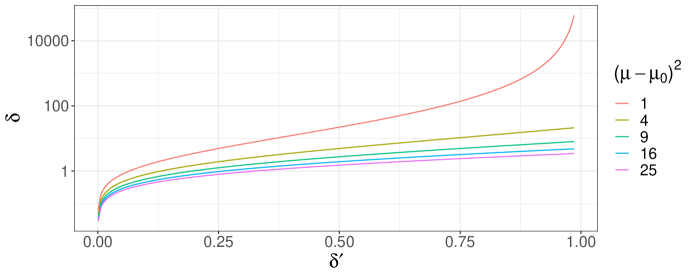
Figure 9: Upper bound on $\delta$ to verify Assumption (A2) in Theorem B.3

Appendix C Description of models

We provide details on the target distributions used in Section 4. For the Rosenbrock, German Credit, Eight Schools, and Item Response models, precise estimates of the mean and variance along each dimension can be found in the Inference Gym (Sountsov et al., 2020). For the Pharmacokinetics example, we compute benchmark means and variances using 2048 chains, each with 1000 warmup and 1000 sampling iterations. We run MCMC using TensorFlow Probability’s implementation of ChEES-HMC (Hoffman et al., 2021). The resulting effective sample size is between 60,000 and 100,000 depending on the parameters. For the bimodal target, the correct mean and variance are worked out analytically.

C.1 Rosenbrock (Dimension = 2)

The Rosenbrock distribution is a nonlinearly transformed normal distribution with highly non-convex level sets; see Equation 1.

C.2 German Credit (Dimension = 25)

“German Credit” is a Bayesian logistic regression model applied to a dataset from a machine learning repository (Dua and Graff, 2017). There are 24 features and an intercept term. The joint distribution over $(\theta,y)$ is

$$\theta \sim \text{normal}(0,I),$$

$$y_{n} \sim \text{Bernoulli}\left(\frac{1}{1+e^{-\theta^{T}x_{n}}}\right),$$

where $I\in\mathbb{R}^{24\times 24}$ is the identity matrix. Our goal is to sample from the posterior distribution $\pi(\theta\mid y)$.

C.3 Eight Schools (Dimension = 10)

“Eight Schools” is a Bayesian hierarchical model describing the effect of a program to train students to perform better on a standardized test, as measured by performance across 8 schools (Rubin, 1981). We estimate the group mean and the population mean and variance. To avoid a funnel shaped posterior density, we use a non-centered parameterization:

$$\mu \sim \text{normal}(5,3)$$

$$\sigma \sim \text{normal}^{+}(0,10)$$

$$\eta_{n} \sim \text{normal}(0,1)$$

$$\theta_{n} = \mu+\eta_{n}\sigma$$

$$y_{n} \sim \text{normal}(\theta_{n},\sigma_{n}),$$

with the posterior distribution taken over $\mu$ and $\eta$.

C.4 Pharmacokinetic (Dimension = 45)

“Pharmacokinetics” is a one-compartment model with first-order absorption from the gut that describes the diffusion of a drug compound inside a patient’s body. Oral administration of a bolus drug dose induces a discrete change in the drug mass inside the patient’s gut. The drug is then absorbed into the central compartment, which represents the blood and organs into which the drug diffuses profusely. This diffusion process is described by the system of differential equations:

$$\frac{\mathrm{d}m_{\text{gut}}}{\mathrm{d}t} = -k_{1}m_{\text{gut}}$$

$$\frac{\mathrm{d}m_{\text{cent}}}{\mathrm{d}t} = k_{1}m_{\text{gut}}-k_{2}m_{\text{cent}},$$

which admits the analytical solution, when $k_{1}\neq k_{2}$,

$$m_{\text{gut}}(t) = m^{0}_{\text{gut}}\exp(-k_{1}t)$$

$$m_{\text{cent}}(t) = \frac{\exp(-k_{2}t)}{k_{1}-k_{2}}\left(m^{0}_{\text{gut}}k_{1}(1-\exp[(k_{2}-k_{1})t]+(k_{1}-k_{2})m^{0}_{\text{cent}})\right).$$

Here $m^{0}_{\text{gut}}$ and $m^{0}_{\text{cent}}$ are the initial conditions at time $t=0$.

A patient typically receives multiple doses. To model this, we solve the differential equations between dosing events, and then update the drug mass in each compartment, essentially resetting the boundary conditions before we resume solving the differential equations. In our example, this means adding $m_{\text{dose}}$, the drug mass administered by each dose, to $m_{\text{gut}}(t)$ at the time of the dosing event. We label the dosing schedule as $x$.

Each patient receives a total of 3 doses, taken every 12 hours. Measurements are taken at times $t=(0.083,0.167,0.25,0.5,0.75,1,1.5,2,3,4,6,8)$ hours after each dosing event.

We simulate data for 20 patients and for each patient, indexed by $n$, we estimate the coefficients $(k_{1}^{n},k_{2}^{n})$. We use a hierarchical prior to pool information between patients and estimate the population parameters $(k_{1}^{\text{pop}},k_{2}^{\text{pop}})$ with a non-centered parameterization. The full Bayesian model is:

hyperpriors:

$$k_{1}^{\text{pop}} \sim \text{lognormal}(\log 1,0.1)$$

$$k_{2}^{\text{pop}} \sim \text{lognormal}(\log 0.3,0.1)$$

$$\sigma_{1} \sim \text{lognormal}(\log 0.15,0.1)$$

$$\sigma_{2} \sim \text{lognormal}(\log 0.35,0.1)$$

$$\sigma \sim \text{lognormal}(-1,1)$$

hierarchical  priors:

$$\eta_{1}^{n} \sim \text{normal}(0,1)$$

$$\eta_{2}^{n} \sim \text{normal}(0,1)$$

$$k_{1}^{n} = k_{1}^{\text{pop}}\exp(\eta_{1}^{n}\sigma_{1})$$

$$k_{2}^{n} = k_{2}^{\text{pop}}\exp(\eta_{2}^{n}\sigma_{2})$$

likelihood:

$$y_{n} \sim \text{lognormal}(\log m_{\text{cent}}(t,k_{1}^{n},k_{2}^{n},x),\sigma).$$

We fit the model on the unconstrained scale, meaning the Markov chains explore the parameter space of, for example, $\log k_{1}^{\text{pop}}\in\mathbb{R}$, rather than $k_{1}^{\text{pop}}\in\mathbb{R}^{+}$.

C.5 Mixture of Gaussians (Dimension = 100)

A mixture of two well-seperated 100-dimensional standard Gaussians,

$$\theta\sim 0.3\ \text{normal}(-\mu,I)+0.7\ \text{normal}(\mu,I),$$

where $\mu$ is the 100-dimensional vector of 5’s.

C.6 Item Response Theory (Dimension = 501)

The posterior of a model to estimate students abilities when taking an exam. There are $J=400$ students and $L=100$ questions. The model parameters are the mean student ability $\delta\in\mathbb{R}$, the ability of each individual student $\boldsymbol{\alpha}\in\mathbb{R}^{J}$ and the difficulty of each question $\boldsymbol{\beta}\in\mathbb{R}^{L}$. The observations are the binary matrix $Y\in\mathbb{R}^{J\times L}$, with $y_{j\ell}$ the response of student $j$ to question $\ell$. The joint distribution is

$$\delta \sim \text{normal}(0.75,1)$$

$$\boldsymbol{\alpha} \sim \text{mormal}(0,I)$$

$$\boldsymbol{\beta} \sim \text{normal}(0,I)$$

$$y_{j\ell} \sim \text{Bernoulli}\left[\text{logit}^{-1}(\alpha_{j}-\beta_{\ell}+\delta)\right].$$

References

- Beskos et al. (2013) Beskos, A., Pillai, N., Roberts, G., Sanz-Serna, J.-M., and Stuart, A. (2013). “Optimal tuning of the hybrid Monte Carlo algorithm.” Bernoulli, 19(5A): 1501–1534.
- Betancourt (2018) Betancourt, M. (2018). “A conceptual introduction to Hamiltonian Monte Carlo.” arXiv:1701.02434v1.
- Brooks and Gelman (1998) Brooks, S. P. and Gelman, A. (1998). “General methods for monitoring convergence of iterative simulations.” Journal of Computational and Graphical Statistics, 7: 434–455.
- Cowles and Carlin (1996) Cowles, M. K. and Carlin, B. P. (1996). “Markov chain Monte Carlo convergence diagnostics: A comparative review.” Journal of the American Statistical Association, 91: 883–904.
- Cowles et al. (1998) Cowles, M. K., Roberts, G. O., and Rosenthal, J. S. (1998). “Possible biases induced by MCMC convergence diagnostics.” Journal of Statistical Computation and Simulation, 64: 87–104.
- Del Moral et al. (2006) Del Moral, P., Doucet, A., and Jasra, A. (2006). “Sequential Monte Carlo samplers.” Journal of the Royal Statistical Society, Series B, 68: 411–436.
-
Dua and Graff (2017)
Dua, D. and Graff, C. (2017).
“UCL machine learning repository.”
URL http://archive.ics.ucl.edu/ml - Flegal et al. (2008) Flegal, J. M., Haran, M., and Jones, G. L. (2008). “Markov chain Monte Carlo: Can we trust the third significant figure?” Statistical Science, 250–260.
- Gardiner (2004) Gardiner, C. W. (2004). Handbook of Stochastic Methods for Physics, Chemistry and the Natural Sciences, 3rd edition. Springer-Verlag, Berlin.
- Gelman et al. (2013) Gelman, A., Carlin, J. B., Stern, H. S., Dunson, D., Vehtari, A., and Rubin, D. B. (2013). Bayesian Data Analysis, 3rd edition. CRC Press.
- Gelman et al. (1997) Gelman, A., Gilks, W. R., and Roberts, G. O. (1997). “Weak convergence and optimal scaling of random walk Metropolis algorithms.” Annals of Applied Probability, 7(1): 110–120.
- Gelman and Hill (2007) Gelman, A. and Hill, J. (2007). Data Analysis Using Regression and Multilevel-Hierarchical Models. Cambridge University Press.
- Gelman and Rubin (1992) Gelman, A. and Rubin, D. B. (1992). “Inference from iterative simulation using multiple sequences (with discussion).” Statistical Science, 7: 457–511.
- Gelman and Shirley (2011) Gelman, A. and Shirley, K. (2011). “Inference from simulations and monitoring convergence.” In Handbook of Markov chain Monte Carlo, chapter 4. CRC Press.
- Geweke (1992) Geweke, J. (1992). “Evaluating the accuracy of sampling-based approaches to the calculation of posterior moments.” In Bayesian Statistics 4, 169–193. Oxford University Press.
- Glynn and Rhee (2014) Glynn, P. W. and Rhee, C.-H. (2014). “Exact estimation for Markov chain equilibrium expectations.” Journal of Applied Probability, 51: 377–389.
- Heng and Jacob (2019) Heng, J. and Jacob, P. E. (2019). “Unbiased Hamiltonian Monte Carlo with couplings.” Biometrika, 106: 287 – 302.
- Hoffman and Sountsov (2022) Hoffman, M. and Sountsov, P. (2022). “Tuning-free generalized Hamiltonian Monte Carlo.” Artificial Intelligence and Statistics.
- Hoffman and Gelman (2014) Hoffman, M. D. and Gelman, A. (2014). “The no-U-turn sampler: Adaptively setting path lengths in Hamiltonian Monte Carlo.” Journal of Machine Learning Research, 15: 1593–1623.
- Hoffman et al. (2021) Hoffman, M. D., Radul, A., and Sountsov, P. (2021). “An adaptive MCMC scheme for setting trajectory lengths in Hamiltonian Monte Carlo.” Artificial Intelligence and Statistics.
- Jacob et al. (2020) Jacob, P. E., O’Leary, J., and Atchadé, Y. F. (2020). “Unbiased Markov chain Monte Carlo methods with couplings.” Journal of the Royal Statistical Society, Series B, 82: 543–600.
- Jones et al. (2006) Jones, G. L., Haran, M., Caffo, B. S., and Neath, R. (2006). “Fixed-width output analysis for Markov chain Monte Carlo.” Journal of the American Statistical Association, 101: 1537–1547.
- Lambert and Vehtari (2022) Lambert, B. and Vehtari, A. (2022). “: A robust MCMC convergence diagnostic with uncertainty using decision tree classifiers.” Bayesian Analysis, 17: 353–379.
- Lao et al. (2020) Lao, J., Suter, C., Langmore, I., Chimisov, C., Saxena, A., Sountsov, P., Moore, D., Saurous, R. A., Hoffman, M. D., and Dillon, J. V. (2020). “tfp.mcmc: Modern Markov chain Monte Carlo tools built for modern hardware.” arXiv:2002.01184.
- Mackay (2003) Mackay, D. J. (2003). Information Theory, Inference, and Learning Algorithms. Cambridge University Press.
- Margossian and Gelman (2023) Margossian, C. C. and Gelman, A. (2023). “For how many iterations should we run Markov chain Monte Carlo.” arXiv:2311.02726.
- Margossian et al. (2022) Margossian, C. C., Zhang, Y., and Gillespie, W. R. (2022). “Flexible and efficient Bayesian pharmacometrics modeling using Stan and Torsten, part I.” CPT: Pharmacometrics & Systems Pharmacology, 11: 1151–1169.
- Moins et al. (2023) Moins, T., Arbel, J., Dutfoy, A., and Girard, S. (2023). “On the use of a local to improve MCMC convergence diagnostic.” Bayesian Analysis.
- Neal (2001) Neal, R. M. (2001). “Annealed importance sampling.” Statistics and Computing, 11: 125–139.
- Neal (2012) — (2012). “MCMC using Hamiltonian dynamics.” In Handbook of Markov Chain Monte Carlo. CRC Press.
- Nguyen et al. (2022) Nguyen, T. D., Trippe, B. L., and Broderick, T. (2022). “Many processors, little time: MCMC for partitions via optimal transport couplings.” Artificial Intelligence and Statistics, 151: 3483–3514.
- Papaspiliopoulos et al. (2007) Papaspiliopoulos, O., Roberts, G. O., and Sköld, M. (2007). “A general framework for the parametrization of hierarchical models.” Statistical Science, 22: 59–73.
- Riabiz et al. (2022) Riabiz, M., Chen, W., Cockayne, J., Swietach, P., Niederer, S. A., Mackey, L., and Oates, C. J. (2022). “Optimal thinning of MCMC output.” Journal of the Royal Statistical Society: Series B, 84: 1059–1081.
- Riou-Durand et al. (2023) Riou-Durand, L., Sountsov, P., Vogrinc, J., Margossian, C. C., and Power, S. (2023). “Adaptive tuning for Metropolis adjusted Langevin trajectories.” Artificial Intelligence and Statistics.
- Riou-Durand and Vogrinc (2022) Riou-Durand, L. and Vogrinc, J. (2022). “Metropolis adjusted Langevin trajectories: A robust alternative to Hamiltonian Monte Carlo.” arXiv:2202.13230.
- Robert and Casella (2004) Robert, C. P. and Casella, G. (2004). Monte Carlo Statistical Methods. Springer.
- Roberts and Rosenthal (1998) Roberts, G. O. and Rosenthal, J. S. (1998). “Optimal scaling of discrete approximations to Langevin diffusions.” Journal of the Royal Statistical Society, Series B, 60: 255–268.
- Rosenbrock (1960) Rosenbrock, H. H. (1960). “An automatic method for finding the greatest or least value of a function.” Computer Journal, 3: 175–184.
- Rosenthal (2000) Rosenthal, J. S. (2000). “Parallel computing and Monte Carlo algorithms.” Far East Journal of Theoretical Statistics, 4: 207–236.
- Rubin (1981) Rubin, D. B. (1981). “Estimation in parallelized randomized experiments.” Journal of Educational Statistics, 6: 377–400.
- Sountsov and Hoffman (2021) Sountsov, P. and Hoffman, M. D. (2021). “Focusing on difficult directions for learning HMC trajectory lengths.” arXiv:2110.11576.
-
Sountsov et al. (2020)
Sountsov, P., Radul, A., and contributors (2020).
“Inference Gym.”
URL https://pypi.org/project/inference_gym - South et al. (2021) South, L. F., Riabiz, M., Teymur, O., and Oates, C. J. (2021). “Post-processing of MCMC.” Annual Review of Statistics and its Application, 9: 1–30.
-
TensorFlow Probability Development Team (2023)
TensorFlow Probability Development Team (2023).
“TensorFlow Probability.”
URL https://www.tensorflow.org/probability - Vats et al. (2019) Vats, D., Flegal, J. M., and Jones, G. L. (2019). “Multivariate output analysis for Markov chain Monte Carlo.” Biometrika, 106: 321–337.
- Vats and Knudson (2021) Vats, D. and Knudson, D. (2021). “Revisiting the Gelman-Rubin diagnostic.” Statistical Science, 36: 518–529.
-
Vehtari (2022)
Vehtari, A. (2022).
“Bayesian workflow book - Digits.”
URL https://avehtari.github.io/casestudies/Digits/digits.html - Vehtari et al. (2021) Vehtari, A., Gelman, A., Simpson, D., Carpenter, B., and Bürkner, P.-C. (2021). “Rank-normalization, folding, and localization: An improved for assessing convergence of MCMC (with discussion).” Bayesian Analysis, 16: 667–718.
- Wakefield (1996) Wakefield, J. (1996). “The Bayesian analysis of population pharmacokinetic models.” Journal of the American Statistical Association, 91: 62–75.
- Zhang et al. (2020) Zhang, Y., Gillespie, B., Bales, B., and Vehtari, A. (2020). “Speed up population Bayesian inference by combining cross-chain warmup and within-chain parallelization.” In American Conference on Pharmacometrics.