Uncertainty in Bayesian Leave-One-Out Cross-Validation Based Model Comparison

Abstract

Leave-one-out cross-validation (LOO-CV) is a popular method for comparing Bayesian models based on their estimated predictive performance on new, unseen, data. As leave-one-out cross-validation is based on finite observed data, there is uncertainty about the expected predictive performance on new data. By modeling this uncertainty when comparing two models, we can compute the probability that one model has a better predictive performance than the other. Modeling this uncertainty well is not trivial, and for example, it is known that the commonly used standard error estimate is often too small. We study the properties of the Bayesian LOO-CV estimator and the related uncertainty estimates when comparing two models. We provide new results of the properties both theoretically in the linear regression case and empirically for multiple different models and discuss the challenges of modeling the uncertainty. We show that problematic cases include: comparing models with similar predictions, misspecified models, and small data. In these cases, there is a weak connection in the skewness of the individual leave-one-out terms and the distribution of the error of the Bayesian LOO-CV estimator. We show that it is possible that the problematic skewness of the error distribution, which occurs when the models make similar predictions, does not fade away when the data size grows to infinity in certain situations. Based on the results, we also provide practical recommendations for the users of Bayesian LOO-CV for model comparison.

Keywords: Bayesian computation, model comparison, leave-one-out cross-validation, uncertainty, asymptotics

1 Introduction

When comparing different Bayesian models, we are often interested in their predictive performance for new, unseen data. We cannot compute the predictive performance for unseen data directly. We can estimate it using, for example, cross-validation (Geisser, 1975; Geisser and Eddy, 1979; Gelfand et al., 1992; Bernardo and Smith, 1994; Gelfand, 1996; Vehtari and Ojanen, 2012) and then, in the model comparison, take into account the uncertainty related to the difference of the predictive performance estimates for the different models (Vehtari and Lampinen, 2002; Vehtari and Ojanen, 2012).

Leave-one-out cross-validation (LOO-CV) has become a popular approach for Bayesian model comparison; For example, loo R package (Vehtari et al., 2022a), which implements a fast LOO-CV computation (Vehtari et al., 2017), has been downloaded more than 3 million times from RStudio CRAN mirror alone. Part of the model comparison in loo package is also to estimate the uncertainty in the difference between the predictive performances of two models. The uncertainty in the predictive performance estimates is due to approximating the unknown future data distribution with a finite number of re-used observations. To draw rigorous conclusions about the model comparison results, we need to assess the accuracy of the estimated uncertainty, a problem that recently also has attracted attention in the frequentist setting (e.g. see Austern and Zhou, 2020; Bayle et al., 2020; Bates et al., 2023). How well does the estimated uncertainty work when repeatedly applied to a new, comparable problem? Can there be some settings in which the uncertainty is, in general, poorly estimated? Are there some general characteristics that make it hard to estimate the uncertainty? In this paper, we carefully analyse these properties and provide practical guidance for modellers in the Bayesian setting.

Figure 1 shows the joint distribution of the difference in the predictive performance and its LOO-CV estimate for multiple data sets in three cases: (1) clear difference in the performance, (2) small difference in the performance, and (3) model misspecification due to outliers in the data. When estimating the related uncertainty in model comparison, it is often assumed that the empirical standard deviation does a good job, such as in the clear case in Figure 1. The behaviour is different in the other two illustrated settings, and the uncertainty estimates can be unreliable in these settings.

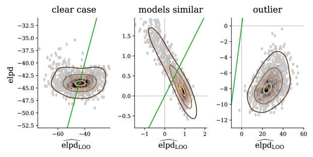
Figure 1: Illustration of the joint distribution of the difference of a predictive performance measure ${\mathrm{elpd}\bigr{(}{\mathrm{M}_{a},\mathrm{M}_{b}}\mid y\bigl{)}}$ and its estimator ${\widehat{\mathrm{elpd}}_{\mathrm{\scriptscriptstyle LOO}}\bigr{(}{\mathrm{M}_{a},\mathrm{M}_{b}}\mid y\bigl{)}}$ in three nested normal linear regression problem settings with $2000$ simulations of $n=128$ observations. Left: model $\mathrm{M}_{b}$ has better predictive performance than model $\mathrm{M}_{a}$. Middle: models have similar predictive performance (Scenario 1) and both distributions of ${\mathrm{elpd}\bigr{(}{\mathrm{M}_{a},\mathrm{M}_{b}}\mid y\bigl{)}}$ and ${\widehat{\mathrm{elpd}}_{\mathrm{\scriptscriptstyle LOO}}\bigr{(}{\mathrm{M}_{a},\mathrm{M}_{b}}\mid y\bigl{)}}$ are highly skewed with a strong negative correlation. Right: the models are misspecified with outliers in the data (Scenario 2), and ${\widehat{\mathrm{elpd}}_{\mathrm{\scriptscriptstyle LOO}}\bigr{(}{\mathrm{M}_{a},\mathrm{M}_{b}}\mid y\bigl{)}}$ is biased. The green diagonal line indicates where ${\mathrm{elpd}\bigr{(}{\mathrm{M}_{a},\mathrm{M}_{b}}\mid y\bigl{)}}={\widehat{\mathrm{elpd}}_{\mathrm{\scriptscriptstyle LOO}}\bigr{(}{\mathrm{M}_{a},\mathrm{M}_{b}}\mid y\bigl{)}}$. The simulated experiments are described in more detail in Section 4.

1.1 Our Contributions

We provide new results for the uncertainty properties in Bayesian LOO-CV model comparison, theoretically and empirically, and illustrate the challenges of quantifying it. Our focus is on analysing the difference in the predictive performance of the LOO-CV estimator of the expected log pointwise predictive density (elpd) in two model comparison.

We formulate the underlying uncertainty and present the two ways of analysing it: the normal approximation and the Bayesian bootstrap (ie. Dirichlet approximation; Rubin, 1981). We analyse the properties of the error distribution and the approximations of that distribution in typical normal linear regression problem settings over possible data sets. Based on this analysis, we identify when these uncertainty estimates can perform poorly: the models make similar predictions (Scenario 1), the models are misspecified with outliers in the data (Scenario 2), or the number of observations is small (Scenario 3). Consequences of these problematic cases are:

1. When the models make similar predictions (Scenario 1), there is not much difference in the predictive performance. Still, the bad calibration makes LOO-CV less accurate for separating tiny effect sizes from zero effect sizes.

2. Model misspecification in model comparison (Scenario 2) should be avoided by proper model checking and expansion before using LOO-CV.

3. LOO-CV can not reliably detect small differences in the predictive performance if the number of observations is small (Scenario 3).

We have derived analytical results for normal linear regression with random covariates, and demonstrate experimentally the same behavior with fixed covariate, hierarchical linear, Poisson generalized linear, and spline models. The underlying reasons and consequences are the same for Bayesian $K$-fold-CV, and we demonstrate the similar behaviour in experimental results. In a non-Bayesian context, Arlot and Celisse (2010) provide several results for different cross-validation approaches, where most of the discussed results are similar to the results presented here. To the best of our knowledge, these are the first results in a Bayesian domain, including pre-asymptotic behaviour.

2 Problem Setting

This section introduces the problem, reviews the current literature and related methodology, and presents the main points of the new results. For a positive integer $n>0$, $y=(y_{1},y_{2},\dots,y_{n})$ is generated from $p_{\text{true}}(y)$, representing the true data generating mechanism for $y$. $y_{i}$ are not assumed to be independent or identically distributed. For evaluating models $\mathrm{M}_{k}$$\in\{{\mathrm{M}_{a}}{},{\mathrm{M}_{b}}{}\}$, we consider the expected log pointwise predictive density (Vehtari and Ojanen, 2012)a measure of predictive accuracy for another data set $\tilde{y}=(\tilde{y}_{1},\tilde{y}_{2},\dots,\tilde{y}_{n})$, independent of $y$, and generated from the same $p_{\text{true}}(y)$ as:

$${\mathrm{elpd}\bigr{(}{\mathrm{M}_{k}}\mid y\bigl{)}} =\sum_{i=1}^{n}\operatorname{E}_{\tilde{y}_{i}}\mathopen{}\mathclose{{}\left[\log p_{\mathrm{M}_{k}}(\tilde{y}_{i}\mid y)}\right]=\sum_{i=1}^{n}\int p_{\mathrm{true}}(\tilde{y}_{i})\log p_{k}(\tilde{y}_{i}\mid y)\mathop{}\kern-2.0pt\mathrm{d}\tilde{y}_{i}\,,$$ (1)

where $\log p_{k}(\tilde{y}_{i}\mid y)$ is the logarithm of the posterior predictive density for the model $\mathrm{M}_{k}$ fitted for data set $y$. The use of the posterior predictive distribution in Equation (1) is specific to the Bayesian setting. In this measure, the observations are considered pointwise to maintain comparability with the given data set (p. 168, Gelman et al., 2013). A summary of notation used in the paper is presented in Table 1. We can use different utility and loss functions, but for simplicity, we use the strictly proper and local log score (Gneiting and Raftery, 2007; Vehtari and Ojanen, 2012) throughout the paper.

For evaluating model $\mathrm{M}_{k}$ in the context of a specific data generating mechanism in general, the respective measure of predictive performance is the expectation of ${\mathrm{elpd}\bigr{(}{\mathrm{M}_{k}}\mid y\bigl{)}}$ over all possible data sets $y$:

$$\text{expected }{\mathrm{elpd}\bigr{(}{\mathrm{M}_{k}}\mid y\bigl{)}}=\operatorname{E}_{y}\mathopen{}\mathclose{{}\left[{\mathrm{elpd}\bigr{(}{\mathrm{M}_{k}}\mid y\bigl{)}}}\right]\,.$$ (2)

The ${\mathrm{elpd}\bigr{(}{\mathrm{M}_{k}}\mid y\bigl{)}}$ in Equation (1), conditioned on $y$, can be considered as an estimate for the measure in Equation (2). The former measure is of interest in application-oriented model building workflow when evaluating or comparing fitted models for a given data. In contrast, the latter is of interest in algorithm-oriented experiments when analysing the performance of models in the context of a problem set in general (e.g. Dietterich, 1998; Bengio and Grandvalet, 2004). This paper primarily focuses on the former measure, which is often useful in the Bayesian setting (Gelman et al., 2020). Differences in these measures and their uncertainties are further discussed in Appendix A.

Although we do not consider data shifts, covariates can be modelled in various ways using the functions defined in (1) and (2). In the experiments, we consider stochastic covariates and observe a similar behaviour with different setups. More discussion of the covariate setup is presented by Vehtari and Lampinen (2002) and Vehtari and Ojanen (2012). For brevity, we omit the covariates most of the time in the notation.

notation	meaning
$n$	number of observations in a data set
$y$	data set of $n$ observations from $p_{\text{true}}(y)$
$\tilde{y}$	another independent analogous data set of $n$ observations from $p_{\text{true}}(y)$
$\mathrm{M}_{k}$	model variable indicating model $k$
$p_{\text{true}}(y)$	distribution representing the true data generating mechanism for $y$ and $\tilde{y}$
$p_{k}(\tilde{y}_{i}\mid y)$	posterior predictive distribution with model ${\mathrm{M}_{k}}$
${\mathrm{elpd}}$	expected log pointwise predictive density utility score single model: ${\mathrm{elpd}\bigr{(}{\mathrm{M}_{k}}\mid y\bigl{)}}=\sum_{i=1}^{n}\int p_{\text{true}}(y_{i})\log p_{\mathrm{M}_{k}}(y_{i}\mid y)\mathop{}\kern-2.0pt\mathrm{d}y_{i}$, model comparison: ${\mathrm{elpd}\bigr{(}{\mathrm{M}_{a},\mathrm{M}_{b}}\mid y\bigl{)}}={\mathrm{elpd}\bigr{(}{\mathrm{M}_{a}}\mid y\bigl{)}}-{\mathrm{elpd}\bigr{(}{\mathrm{M}_{b}}\mid y\bigl{)}}$
${\widehat{\mathrm{elpd}}_{\mathrm{\scriptscriptstyle LOO}}}$	LOO-CV approximation to ${\mathrm{elpd}}$ single model: ${\widehat{\mathrm{elpd}}_{\mathrm{\scriptscriptstyle LOO}}\bigr{(}{\mathrm{M}_{k}}\mid y\bigl{)}}=\sum_{i=1}^{n}\log p_{\mathrm{M}_{k}}(y_{i}\mid y_{-i})$, model comparison: ${\widehat{\mathrm{elpd}}_{\mathrm{\scriptscriptstyle LOO}}\bigr{(}{\mathrm{M}_{a},\mathrm{M}_{b}}\mid y\bigl{)}}={\widehat{\mathrm{elpd}}_{\mathrm{\scriptscriptstyle LOO}}\bigr{(}{\mathrm{M}_{a}}\mid y\bigl{)}}-{\widehat{\mathrm{elpd}}_{\mathrm{\scriptscriptstyle LOO}}\bigr{(}{\mathrm{M}_{b}}\mid y\bigl{)}}$
${\mathrm{err}_{\mathrm{\scriptscriptstyle LOO}}}$	LOO-CV approximation error for ${\mathrm{elpd}\bigr{(}\cdots\mid y\bigl{)}}$: ${\mathrm{err}_{\mathrm{\scriptscriptstyle LOO}}\bigr{(}\cdots\mid y\bigl{)}}={\widehat{\mathrm{elpd}}_{\mathrm{\scriptscriptstyle LOO}}\bigr{(}\cdots\mid y\bigl{)}}-{\mathrm{elpd}\bigr{(}\cdots\mid y\bigl{)}}$
$p({\mathrm{err}_{\mathrm{\scriptscriptstyle LOO}}})$	oracle distribution of uncertainty in ${\mathrm{err}_{\mathrm{\scriptscriptstyle LOO}}}$
$\hat{p}({\mathrm{err}_{\mathrm{\scriptscriptstyle LOO}}})$	approximate distribution $\hat{p}({\mathrm{err}_{\mathrm{\scriptscriptstyle LOO}}})\approx p({\mathrm{err}_{\mathrm{\scriptscriptstyle LOO}}})$
${\widehat{\mathrm{SE}}_{\mathrm{\scriptscriptstyle LOO}}}$	estimator for the standard deviation of ${\widehat{\mathrm{elpd}}_{\mathrm{\scriptscriptstyle LOO}}\bigr{(}\cdots\mid y\bigl{)}}$

Table 1: Notation used.

2.1 Bayesian Cross-Validation

As the true data generating mechanism $p_{\text{true}}(y)$ is usually unknown, (1) needs to be approximated (Bernardo and Smith, 1994; Vehtari and Ojanen, 2012). If we had independent test data $\tilde{y}=(\tilde{y}_{1},\tilde{y}_{2},\dots,\tilde{y}_{n})\sim p_{\mathrm{true}}(\tilde{y})$ we could estimate (1) as

$$\widehat{\mathrm{elpd}}_{\mathrm{test}}({\mathrm{M}_{k}}\mid{y})=\sum_{i=1}^{n}\log p_{\mathrm{M}_{k}}\mathopen{}\mathclose{{}\left(\tilde{y}_{i}\mid y}\right).$$ (3)

This can be considered as a finite sample Monte Carlo estimate of (1). As the terms are independent and if we assume their distribution has finite variance, we could assess the accuracy of this estimate with the usual Monte Carlo error estimates.

When independent test data ($\tilde{y}$) are not available, which is often the case in practice, a popular strategy is cross-validation (CV), in which a finite number of observations are re-used as a proxy for the unobserved independent data (Geisser, 1975). The data is divided into parts used as out-of-sample validation sets on the model fitted using the remaining observations. In $K$-fold CV, the data is divided evenly into $K$ parts, and in leave-one-out CV (LOO-CV), $K=n$, so that every observation is one validation set. Using LOO-CV, we approximate ${\mathrm{elpd}\bigr{(}{\mathrm{M}_{k}}\mid y\bigl{)}}$ as

$${\widehat{\mathrm{elpd}}_{\mathrm{\scriptscriptstyle LOO}}\bigr{(}{\mathrm{M}_{k}}\mid y\bigl{)}} =\sum_{i=1}^{n}\log p_{\mathrm{M}_{k}}\mathopen{}\mathclose{{}\left(y_{i}\mid y_{-i}}\right)\,,$$ (4)

where

$$\log p_{\mathrm{M}_{k}}\big{(}y_{i}\big{|}y_{-i}\big{)} =\log\int p_{\mathrm{M}_{k}}\big{(}y_{i}\big{|}\theta\big{)}p_{\mathrm{M}_{k}}\big{(}\theta\big{|}y_{-i}\big{)}\mathop{}\kern-2.0pt\mathrm{d}\theta$$ (5)

is the LOO predictive log density for the $i$th observation $y_{i}$ with model $\mathrm{M}_{k}$, given the data except the $i$th observation, denoted as $y_{-i}$. The bias of (4) tends to decrease when $n$ grows (Watanabe, 2010). The naive approach would fit the model separately for each fold $p_{k}\big{(}y_{i}\big{|}y_{-i}\big{)}$. In practice, we use more efficient methods such as Pareto smoothed importance sampling (Vehtari et al., 2022b), implicitly adaptive importance sampling (Paananen et al., 2021) and sub-sampling (Magnusson et al., 2019, 2020) to estimate ${\mathrm{elpd}\bigr{(}{\mathrm{M}_{k}}\mid y\bigl{)}}$ more efficiently.

Model comparison

For comparing two models, $\mathrm{M}_{a}$ and $\mathrm{M}_{b}$, given the same collection data $y$, we estimate the difference in their expected predictive accuracy,

$${\mathrm{elpd}\bigr{(}{\mathrm{M}_{a},\mathrm{M}_{b}}\mid y\bigl{)}} ={\mathrm{elpd}\bigr{(}{\mathrm{M}_{a}}\mid y\bigl{)}}-{\mathrm{elpd}\bigr{(}{\mathrm{M}_{b}}\mid y\bigl{)}}$$ (6)

as

$${\widehat{\mathrm{elpd}}_{\mathrm{\scriptscriptstyle LOO}}\bigr{(}{\mathrm{M}_{a},\mathrm{M}_{b}}\mid y\bigl{)}} ={\widehat{\mathrm{elpd}}_{\mathrm{\scriptscriptstyle LOO}}\bigr{(}{\mathrm{M}_{a}}\mid y\bigl{)}}-{\widehat{\mathrm{elpd}}_{\mathrm{\scriptscriptstyle LOO}}\bigr{(}{\mathrm{M}_{b}}\mid y\bigl{)}}$$

$$=\sum^{n}_{i=1}\mathopen{}\mathclose{{}\left(\log p_{\mathrm{M}_{a}}\big{(}y_{i}\big{|}y_{-i}\big{)}-\log p_{\mathrm{M}_{b}}\big{(}y_{i}\big{|}y_{-i}\big{)}}\right)$$

$$=\sum^{n}_{i=1}{\widehat{\mathrm{elpd}}_{\mathrm{\scriptscriptstyle LOO},\,i}\bigr{(}{\mathrm{M}_{a},\mathrm{M}_{b}}\mid y\bigl{)}}\,.$$ (7)

In practice, the objective of a model comparison problem is usually to infer which model has better predictive performance for a given data, indicated by the sign of the difference.

2.2 Uncertainty in Cross-Validation Estimators

If we knew $p_{\text{true}}(y)$ (or had an infinite number of observations from it), we could compute (1) and corresponding model comparison value with arbitrary accuracy, and there would not be any uncertainty. Giiven independent test data of size $n$, we could estimate the uncertainty about (1) as a Monte Carlo error estimate for (3), both for individual models and in model comparison. Assuming the distributions of terms $\log p_{\mathrm{M}_{k}}\mathopen{}\mathclose{{}\left(\tilde{y}_{i}\mid y}\right)$ have finite variance, then the error distributions would converge towards a normal distribution. However, in the finite case, these error distributions can be far from normal. We can compute Monte Carlo error estimate for ${\widehat{\mathrm{elpd}}_{\mathrm{\scriptscriptstyle LOO}}\bigr{(}{\mathrm{M}_{k}}\mid y\bigl{)}}$ (4) and ${\widehat{\mathrm{elpd}}_{\mathrm{\scriptscriptstyle LOO}}\bigr{(}{\mathrm{M}_{a},\mathrm{M}_{b}}\mid y\bigl{)}}$ (7) in the same way. These Monte Carlo error estimates can be considered describing the epistemic uncertainty about the true ${\mathrm{elpd}\bigr{(}{\mathrm{M}_{k}}\mid y\bigl{)}}$ and ${\mathrm{elpd}\bigr{(}{\mathrm{M}_{a},\mathrm{M}_{b}}\mid y\bigl{)}}$.

In the two model comparison, we define the error in the LOO-CV estimate as

$${\mathrm{err}_{\mathrm{\scriptscriptstyle LOO}}\bigr{(}{\mathrm{M}_{a},\mathrm{M}_{b}}\mid y\bigl{)}}={\widehat{\mathrm{elpd}}_{\mathrm{\scriptscriptstyle LOO}}\bigr{(}{\mathrm{M}_{a},\mathrm{M}_{b}}\mid y\bigl{)}}-{\mathrm{elpd}\bigr{(}{\mathrm{M}_{a},\mathrm{M}_{b}}\mid y\bigl{)}}.$$ (8)

We present the uncertainty about the error over possible data sets with distribution $p({\mathrm{err}_{\mathrm{\scriptscriptstyle LOO}}\bigr{(}{\mathrm{M}_{a},\mathrm{M}_{b}}\mid y\bigl{)}})$. Later in this section, we present two methods to approximate this distribution. In this work, we focus on analysing the properties of these approximations with simulation studies where the data generating mechanism $p_{\text{true}}(y)$ is known. Thus, we can compare the approximated distribution $\hat{p}({\mathrm{err}_{\mathrm{\scriptscriptstyle LOO}}\bigr{(}{\mathrm{M}_{a},\mathrm{M}_{b}}\mid y\bigl{)}})$ to the actual known values ${\mathrm{err}_{\mathrm{\scriptscriptstyle LOO}}\bigr{(}{\mathrm{M}_{a},\mathrm{M}_{b}}\mid y\bigl{)}}$ and the true “oracle” distribution $p({\mathrm{err}_{\mathrm{\scriptscriptstyle LOO}}\bigr{(}{\mathrm{M}_{a},\mathrm{M}_{b}}\mid y\bigl{)}})$. The true distribution $p({\mathrm{err}_{\mathrm{\scriptscriptstyle LOO}}\bigr{(}{\mathrm{M}_{a},\mathrm{M}_{b}}\mid y\bigl{)}})$ is not available in real world applications.

We use the probability integral transform (PIT) method (see e.g. Gneiting et al., 2007; Säilynoja et al., 2021) to analyse how well $\hat{p}({\mathrm{err}_{\mathrm{\scriptscriptstyle LOO}}\bigr{(}{\mathrm{M}_{a},\mathrm{M}_{b}}\mid y\bigl{)}})$ is calibrated with respect to $p({\mathrm{err}_{\mathrm{\scriptscriptstyle LOO}}\bigr{(}{\mathrm{M}_{a},\mathrm{M}_{b}}\mid y\bigl{)}})$. By simulating many data sets $y$ from known $p_{\text{true}}(y)$, PIT values from a perfectly calibrated $\hat{p}({\mathrm{err}_{\mathrm{\scriptscriptstyle LOO}}\bigr{(}{\mathrm{M}_{a},\mathrm{M}_{b}}\mid y\bigl{)}})$ would be uniform.

For certain simple data-generating mechanisms and models, we can analytically derive the moments of $p({\mathrm{err}_{\mathrm{\scriptscriptstyle LOO}}\bigr{(}{\mathrm{M}_{a},\mathrm{M}_{b}}\mid y\bigl{)}})$, and compare them to the moments of the approximated uncertainty $\hat{p}({\mathrm{err}_{\mathrm{\scriptscriptstyle LOO}}\bigr{(}{\mathrm{M}_{a},\mathrm{M}_{b}}\mid y\bigl{)}})$ to get insights into why the calibration can be far from perfect in some scenarios. Usual methods to construct $\hat{p}({\mathrm{err}_{\mathrm{\scriptscriptstyle LOO}}\bigr{(}{\mathrm{M}_{a},\mathrm{M}_{b}}\mid y\bigl{)}})$ are the normal approximation and the Bayesian bootstrap (Vehtari and Lampinen, 2002; Vehtari and Ojanen, 2012; Yao et al., 2018). The normal and the Bayesian bootstrap methods are introduced in the following sections and discussed in more detail in Appendix C. In addition of considering $\hat{p}({\mathrm{err}_{\mathrm{\scriptscriptstyle LOO}}\bigr{(}{\mathrm{M}_{a},\mathrm{M}_{b}}\mid y\bigl{)}})$, we can also consider $\hat{p}({\mathrm{elpd}\bigr{(}{\mathrm{M}_{a},\mathrm{M}_{b}}\mid y\bigl{)}})$ which has the same shape, but centered at ${\widehat{\mathrm{elpd}}_{\mathrm{\scriptscriptstyle LOO}}\bigr{(}{\mathrm{M}_{a},\mathrm{M}_{b}}\mid y\bigl{)}}$.

We consider also the distribution of ${\widehat{\mathrm{elpd}}_{\mathrm{\scriptscriptstyle LOO}}\bigr{(}{\mathrm{M}_{a},\mathrm{M}_{b}}\mid y\bigl{)}}$ as a statistic over possible data sets $y$, and call it the sampling distribution. This follows the common definition used in frequentist statistics.

Normal Approximation

The normal approximation approach is established under the assumption that the distribution of the terms ${\widehat{\mathrm{elpd}}_{\mathrm{\scriptscriptstyle LOO},\,i}\bigr{(}{\mathrm{M}_{a},\mathrm{M}_{b}}\mid y\bigl{)}}$ has finite variance, and according to the central limit theorem, the distribution of the sum of these terms approaches a normal distribution. The normal approximation can be formulated as

$$\hat{p}({\mathrm{elpd}\bigr{(}{\mathrm{M}_{a},\mathrm{M}_{b}}\mid y\bigl{)}}) =\operatorname{N}\mathopen{}\mathclose{{}\left({\widehat{\mathrm{elpd}}_{\mathrm{\scriptscriptstyle LOO}}\bigr{(}{\mathrm{M}_{a},\mathrm{M}_{b}}\mid y\bigl{)}},\,{\widehat{\mathrm{SE}}_{\mathrm{\scriptscriptstyle LOO}}\bigr{(}{\mathrm{M}_{a},\mathrm{M}_{b}}\mid y\bigl{)}}}\right)\,,$$ (9)

where $\operatorname{N}(\mu,\sigma)$ is the normal distribution, ${\widehat{\mathrm{elpd}}_{\mathrm{\scriptscriptstyle LOO}}\bigr{(}{\mathrm{M}_{a},\mathrm{M}_{b}}\mid y\bigl{)}}$ is the sample approximation of the mean; and ${\widehat{\mathrm{SE}}_{\mathrm{\scriptscriptstyle LOO}}\bigr{(}{\mathrm{M}_{a},\mathrm{M}_{b}}\mid y\bigl{)}}$ is an estimator for the standard error of ${\widehat{\mathrm{elpd}}_{\mathrm{\scriptscriptstyle LOO}}\bigr{(}{\mathrm{M}_{a},\mathrm{M}_{b}}\mid y\bigl{)}}$ defined as:

$${\widehat{\mathrm{SE}}_{\mathrm{\scriptscriptstyle LOO}}\bigr{(}{\mathrm{M}_{a},\mathrm{M}_{b}}\mid y\bigl{)}}=\mathopen{}\mathclose{{}\left(\frac{n}{n-1}\sum_{i=1}^{n}\biggl{(}{\widehat{\mathrm{elpd}}_{\mathrm{\scriptscriptstyle LOO},\,i}\bigr{(}{\mathrm{M}_{a},\mathrm{M}_{b}}\mid y\bigl{)}}-\frac{1}{n}\sum_{j=1}^{n}{\widehat{\mathrm{elpd}}_{\mathrm{\scriptscriptstyle LOO},\,j}\bigr{(}{\mathrm{M}_{a},\mathrm{M}_{b}}\mid y\bigl{)}}\biggr{)}^{2}}\right)^{1/2}.$$ (10)

Comparing to (8), it can be seen that (10) does not consider the variability caused by the term ${\mathrm{elpd}\bigr{(}{\mathrm{M}_{a},\mathrm{M}_{b}}\mid\tilde{y}\bigl{)}}$ over possible data sets. This central problem in the approximation of the uncertainty is discussed in Section 2.3. The approximated uncertainty can be used to further estimate $\hat{p}\mathopen{}\mathclose{{}\left({\mathrm{elpd}\bigr{(}{\mathrm{M}_{a},\mathrm{M}_{b}}\mid y\bigl{)}}>0}\right)$, the probability that model $\mathrm{M}_{a}$ is better than model $\mathrm{M}_{b}$ in the context of the uncertainty of the LOO-CV estimate.

Bayesian Bootstrap Approximation

An alternative is to use the Dirichlet distribution to model the unknown data distribution and Bayesian bootstrap (BB) (Rubin, 1981; Vehtari and Lampinen, 2002) to construct the distribution for the sum of the terms in $\hat{p}({\mathrm{elpd}\bigr{(}{\mathrm{M}_{a},\mathrm{M}_{b}}\mid y\bigl{)}})$. In BB a sample from $n$-dimensional Dirichlet distribution is used to form weighted sums of the pointwise LOO-CV terms ${\widehat{\mathrm{elpd}}_{\mathrm{\scriptscriptstyle LOO},\,i}\bigr{(}{\mathrm{M}_{a},\mathrm{M}_{b}}\mid y\bigl{)}}$. Weng (1989) shows that bootstrap with Dirichlet weights produces a more accurate posterior approximation than normal approximation or bootstrap with multinomial weights. The obtained sample represents the uncertainty $\hat{p}({\mathrm{elpd}\bigr{(}{\mathrm{M}_{a},\mathrm{M}_{b}}\mid y\bigl{)}})$.

2.3 Problems in Estimating the Uncertainty

Arlot and Celisse (2010, Section 5.2.1) discuss how the stability of the learning algorithm affects the variance, where CV estimators can have high variance over possible data sets which affects also the difference ${\widehat{\mathrm{elpd}}_{\mathrm{\scriptscriptstyle LOO}}\bigr{(}{\mathrm{M}_{a},\mathrm{M}_{b}}\mid y\bigl{)}}$. As log score utility is smooth and integration over the posterior tends to smooth sharp changes, Bayesian LOO-CV tends to have lower variance than Bayesian $K$-fold CV, which has been experimentally demonstrated, for example, by Vehtari et al. (2017). The high variability of LOO-CV estimators makes it essential to consider the uncertainty in model comparison. The commonly used Normal and BB approximations (see Section 2.2) are easy to compute, but they have several limitations. In the following, we review the main previously known challenges related to the uncertainty of the LOO-CV in model comparison.

No Unbiased Estimator for the Variance

First, as shown by Bengio and Grandvalet (2004), there is no generally unbiased estimator for the variance of ${\widehat{\mathrm{elpd}}_{\mathrm{\scriptscriptstyle LOO}}\bigr{(}{\mathrm{M}_{k}}\mid y\bigl{)}}$ nor ${\widehat{\mathrm{elpd}}_{\mathrm{\scriptscriptstyle LOO}}\bigr{(}{\mathrm{M}_{a},\mathrm{M}_{b}}\mid y\bigl{)}}$. As each observation is part of $n-1$ “training” sets, the contributing terms in ${\widehat{\mathrm{elpd}}_{\mathrm{\scriptscriptstyle LOO}}\bigr{(}\cdot\mid y\bigl{)}}$ are not independent, and the naive variance estimator used to compute ${\widehat{\mathrm{SE}}_{\mathrm{\scriptscriptstyle LOO}}\bigr{(}{\mathrm{M}_{a},\mathrm{M}_{b}}\mid y\bigl{)}})$ in (10) is biased (see e.g. Sivula et al., 2022). Even though it is possible to derive unbiased estimators for certain models (Sivula et al., 2022), an exact unbiased estimator is not required for useful approximations. It is problematic that based on experimental results, the variance of ${\widehat{\mathrm{elpd}}_{\mathrm{\scriptscriptstyle LOO}}\bigr{(}{\mathrm{M}_{k}}\mid y\bigl{)}}$ can be greatly underestimated when $n$ is small, if the model is misspecified, or there are outliers in the data (Bengio and Grandvalet, 2004; Varoquaux et al., 2017; Varoquaux, 2018). We show that under-estimation of the variance also holds in the case of model comparison with ${\widehat{\mathrm{elpd}}_{\mathrm{\scriptscriptstyle LOO}}\bigr{(}{\mathrm{M}_{a},\mathrm{M}_{b}}\mid y\bigl{)}}$, and even more so for models with very similar predictions.

Potentially High Skewness

Second, as demonstrated in Figure 1, the distribution $p({\widehat{\mathrm{elpd}}_{\mathrm{\scriptscriptstyle LOO}}\bigr{(}{\mathrm{M}_{a},\mathrm{M}_{b}}\mid y\bigl{)}})$ can be highly skewed, and we may doubt the accuracy of the normal approximation in a finite data case. We show that estimating the skewness of ${\widehat{\mathrm{elpd}}_{\mathrm{\scriptscriptstyle LOO}}\bigr{(}{\mathrm{M}_{a},\mathrm{M}_{b}}\mid y\bigl{)}}$ from the contributing terms ${\widehat{\mathrm{elpd}}_{\mathrm{\scriptscriptstyle LOO},\,i}\bigr{(}{\mathrm{M}_{a},\mathrm{M}_{b}}\mid y\bigl{)}}$ is also a hard task. To capture higher moments, Vehtari and Lampinen (2002) proposed to use BB approximation (Rubin, 1981), which in theory should be more accurate (Weng, 1989), but it also has problems with higher moments and heavy-tailed distributions in the finite case, as the approximation is essentially truncated at the extreme observed values (as already noted by Rubin, 1981). Furthermore, as later discussed in this section, the mismatch between distributions $p({\mathrm{err}_{\mathrm{\scriptscriptstyle LOO}}\bigr{(}{\mathrm{M}_{a},\mathrm{M}_{b}}\mid y\bigl{)}})$ and the distribution of the contributing terms ${\widehat{\mathrm{elpd}}_{\mathrm{\scriptscriptstyle LOO},\,i}\bigr{(}{\mathrm{M}_{a},\mathrm{M}_{b}}\mid y\bigl{)}}$, means that we are not able to obtain useful information about the higher moments. There was no practical benefit of using Bayesian bootstrap instead of normal approximation in our experiments.

Mismatch Between Contributing Terms and Error Distributions

Third, we construct the approximated distribution $\hat{p}({\mathrm{elpd}\bigr{(}{\mathrm{M}_{a},\mathrm{M}_{b}}\mid y\bigl{)}})$ using information available in the terms ${\widehat{\mathrm{elpd}}_{\mathrm{\scriptscriptstyle LOO},\,i}\bigr{(}{\mathrm{M}_{a},\mathrm{M}_{b}}\mid y\bigl{)}}$, but we show that the connection between the true distribution $p({\mathrm{err}_{\mathrm{\scriptscriptstyle LOO}}\bigr{(}{\mathrm{M}_{a},\mathrm{M}_{b}}\mid y\bigl{)}})$ and the distribution of the terms ${\widehat{\mathrm{elpd}}_{\mathrm{\scriptscriptstyle LOO},\,i}\bigr{(}{\mathrm{M}_{a},\mathrm{M}_{b}}\mid y\bigl{)}}$ can be weak. This is because, in addition to ${\widehat{\mathrm{elpd}}_{\mathrm{\scriptscriptstyle LOO},\,i}\bigr{(}{\mathrm{M}_{a},\mathrm{M}_{b}}\mid y\bigl{)}}$, the distribution $p({\mathrm{err}_{\mathrm{\scriptscriptstyle LOO}}\bigr{(}{\mathrm{M}_{a},\mathrm{M}_{b}}\mid y\bigl{)}})$ is affected by the dependent term ${\mathrm{elpd}\bigr{(}{\mathrm{M}_{a},\mathrm{M}_{b}}\mid y\bigl{)}}$, as seen in (8). We show that even if the true distribution of the contributing terms ${\widehat{\mathrm{elpd}}_{\mathrm{\scriptscriptstyle LOO},\,i}\bigr{(}{\mathrm{M}_{a},\mathrm{M}_{b}}\mid y\bigl{)}}$ is known, it may not help in producing a good approximation for $p({\mathrm{err}_{\mathrm{\scriptscriptstyle LOO}}\bigr{(}{\mathrm{M}_{a},\mathrm{M}_{b}}\mid y\bigl{)}})$.

Asymptotic inconsistency

Fourth, in a non-Bayesian context, Shao (1993) shows that for nested linear models with the true model included, squared prediction error LOO-CV is model selection inconsistent. That is, the probability of choosing the true model does not converge to 1 when the number of observations $n\rightarrow\infty$ (see, also Arlot and Celisse, 2010, Section 7.1). Asymptotically, all the models that include the true model will have the same predictive performance. Due to the variance in the LOO-CV estimator, there is a non-zero probability that we will select a bigger model than the true model. Shao’s result, based on least squares, point prediction and squared errors, is an asymptotic analysis for a non-Bayesian problem. Although, Shao (1993) reflect the fact that also in Bayesian analysis, using the predictive distribution and the log score in a finite situation, the variance in LOO-CV could make it difficult to compare models which have very similar predictive performance. We provide finite case and asymptotic results in Bayesian context and analyse also higher moments of the uncertainty.

Effect of Model Misspecification

Finally, model misspecification and outliers in the data affect the results in complex ways. Bengio and Grandvalet (2004) demonstrate that given a well-specified model without outliers in the data, the correlation between elpd for individual observations may subside as $n$ grows. They also demonstrate that if the model is misspecified and there are outliers in the data, the correlation may significantly affect the total variance even with large $n$. We show that outliers affect the constants in the moment terms, and thus larger $n$ is required to achieve good accuracy.

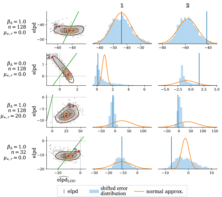
Figure 2: Demonstration of the estimated uncertainty in a simulated normal linear regression with different cases. Two realisations in each setting are illustrated in more detail: (1) near the mode and (2) at the tail area of the distribution of the predictive performance and its estimate. Parameter $\beta_{\Delta}$ controls the difference in the predictive performance of the models, $n$ is the size of the data set, and $\mu_{\star,\mathrm{r}}$ is the magnitude of an outlier observation. The experiments are described in Section 4. In the first column, the green diagonal line indicates where ${\mathrm{elpd}\bigr{(}{\mathrm{M}_{a},\mathrm{M}_{b}}\mid y\bigl{)}}={\widehat{\mathrm{elpd}}_{\mathrm{\scriptscriptstyle LOO}}\bigr{(}{\mathrm{M}_{a},\mathrm{M}_{b}}\mid y\bigl{)}}$ and the brown-yellow lines illustrate density isocontours estimated with the Gaussian kernel method with bandwidth 0.5. In the second and third columns, the yellow line shows the normal approximation to the uncertainty, and the blue histogram illustrates the corresponding target, the error distribution located at ${\widehat{\mathrm{elpd}}_{\mathrm{\scriptscriptstyle LOO}}\bigr{(}{\mathrm{M}_{a},\mathrm{M}_{b}}\mid y\bigl{)}}$.

Demonstration of the Estimated Uncertainty

Figure 2 demonstrates different realisations of normal approximations to the uncertainty in several simulated linear regression cases. We later show empirically that similar behaviour also occurs with other problem settings. The selected example realisations represent the behaviour near the mode and at the tail area of the distribution of the predictive performance and its estimate. The selected examples show that the estimated uncertainty can be good in clear model comparison cases, but it can also incorrectly indicate similarity or difference in the predictive performance. In some situations, an overestimated uncertainty strengthens the belief of uncertainty of the sign of the difference. This behaviour can be desirable or undesirable depending on the situation. Although theoretically, BB has better asymptotic properties than the normal approximation (Weng, 1989), the approximation to the uncertainty was quite similar to the normal approximation in all the experimented cases. Thus the results are not illustrated in the figure.

1. In the first case, the shape of the normal approximation $\hat{p}({\mathrm{elpd}\bigr{(}{\mathrm{M}_{a},\mathrm{M}_{b}}\mid y\bigl{)}})$ is close to the shape of the error distribution $p({\mathrm{err}_{\mathrm{\scriptscriptstyle LOO}}\bigr{(}{\mathrm{M}_{a},\mathrm{M}_{b}}\mid y\bigl{)}})$, and it correctly indicates that the model ${\mathrm{M}_{b}}$ has better predictive performance.

2. In the second case, the models have similar predictive performance (Scenario 1), and the distribution $p({\mathrm{elpd}\bigr{(}{\mathrm{M}_{a},\mathrm{M}_{b}}\mid y\bigl{)}})$ is skewed. In the case near the mode, the uncertainty is underestimated, and the normal approximation $\hat{p}({\mathrm{elpd}\bigr{(}{\mathrm{M}_{a},\mathrm{M}_{b}}\mid y\bigl{)}})$ incorrectly indicates that the model ${\mathrm{M}_{a}}$ has slightly better predictive performance. In the case of the tail area, the uncertainty is overestimated, which is not harmful as it emphasises the uncertainty of the sign of the performance difference.

3. In the third case, there is an outlier observation in the data set (Scenario 2) and the estimator ${\widehat{\mathrm{elpd}}_{\mathrm{\scriptscriptstyle LOO}}\bigr{(}{\mathrm{M}_{a},\mathrm{M}_{b}}\mid y\bigl{)}}$ is biased. Poor calibration is inevitable with any symmetric approximate distribution. The variance in the uncertainty is overestimated in both cases. However, precise variance estimation would narrow the estimated uncertainty, making it o have worse calibration.

4. In the last case, the number of observations is small (Scenario 3). The case near the mode illustrates an undesirable overestimation of the uncertainty. The model ${\mathrm{M}_{b}}$ has better predictive performance, and the difference is estimated correctly, but the overestimated uncertainty indicates that the sign of the difference is not certain. In the tail, the uncertainty is underestimated, suggesting that the models might have equally good predictive performance. In reality, the model ${\mathrm{M}_{b}}$ is better.

While inaccurately representing $p({\mathrm{err}_{\mathrm{\scriptscriptstyle LOO}}\bigr{(}{\mathrm{M}_{a},\mathrm{M}_{b}}\mid y\bigl{)}})$ in some cases, the obtained approximated $\hat{p}({\mathrm{elpd}\bigr{(}{\mathrm{M}_{a},\mathrm{M}_{b}}\mid y\bigl{)}})$ can be useful in practice if the problematic cases are considered carefully as discussed in Section 1.1 and summarised in Section 5. More detailed experiments are presented in Section 4.

3 Theoretical Analysis using Bayesian Linear Regression

To study the uncertainty related to the approximation error, we examine it given a normal linear regression model as the known data generating mechanism. Let $p_{\text{true}}(y)$ be

$$y=X\beta+\varepsilon,$$

$$\varepsilon\sim\operatorname{N}\mathopen{}\mathclose{{}\left(\mu_{\star},\;\Sigma_{\star}}\right),$$ (11)

where $y\in\mathbb{R}^{n}$, and $X\in\mathbb{R}^{n\times d}$ are the independent variable and design matrix respectively, $\beta\in\mathbb{R}^{d}$ a vector of the unknown covariate effect parameters, $\varepsilon\in\mathbb{R}^{n}$ is the vector of errors normally distributed and denoted as residual noise, with underlying parameters $\mu_{\star}\in\mathbb{R}^{n}$, and $\Sigma_{\star}\in\mathbb{R}^{n\times n}$ a positive definite matrix, and hence there exist a unique matrix $\Sigma_{\star}^{1/2}$ such that $\Sigma_{\star}^{1/2}\Sigma_{\star}^{1/2}=\Sigma_{\star}$. Let the vector $\sigma_{\star}\in\mathbb{R}^{n}$ contain the square roots of the diagonal of $\Sigma_{\star}$. The process can be modified to generate outliers by controlling the magnitude of the respective values in $\mu_{\star}$. Under this model, we can analytically study the effect of the uncertainty in different situations.

3.1 Models

We compare two normal linear regression models $\mathrm{M}_{a}$ and $\mathrm{M}_{b}$, with subsets of covariates $d_{\mathrm{M}_{a}}$ and $d_{\mathrm{M}_{b}}$ respectively. We assume $d_{\mathrm{M}_{a}}\neq d_{\mathrm{M}_{b}}$. Otherwise, ${\mathrm{elpd}\bigr{(}{\mathrm{M}_{a},\mathrm{M}_{b}}\mid y\bigl{)}}$ and ${\widehat{\mathrm{elpd}}_{\mathrm{\scriptscriptstyle LOO}}\bigr{(}{\mathrm{M}_{a},\mathrm{M}_{b}}\mid y\bigl{)}}$ would be trivially 0. We write the models ${\mathrm{M}_{k}}\in\{{\mathrm{M}_{a}},{\mathrm{M}_{b}}\}$ as

$$y|\widehat{\beta}_{d_{\mathrm{M}_{k}}},X_{[\boldsymbol{\cdot},{d_{k}}]},\tau \sim\operatorname{N}\mathopen{}\mathclose{{}\left(X_{[\boldsymbol{\cdot},{d_{k}}]}\widehat{\beta}_{d_{\mathrm{M}_{k}}},\;\tau^{2}\mathrm{I}}\right)\,,$$ (12)

where $\widehat{\beta}_{d_{k}}$ is the respective estimated unknown model parameter. In both models, the noise variance $\tau^{2}$ is fixed and a non-informative uniform prior on $\widehat{\beta}_{d_{k}}$ is applied. The resulting posterior and posterior predictive distributions are normal (Appendix D).

3.2 Controlling the Similarity of the Predictive Performances

Let $\beta_{\Delta}$ denote the effects of the non-shared covariates, that is, the covariates included in one model but not in the other. If $\beta_{\Delta}=0$, both models are similar in the sense that they both include the same model with most non-zero effects, but the noise in the non-effective covariates affects the resulting predictive performance. Situations, in which the models are close in predictive performance, often arise in practice, for example, in variable selection. As discussed in Section 2, analysing the uncertainty in the model comparison can be problematic in these situations (Scenario 1).

3.3 Properties for Finite Data

By applying the specified model setting, data generating mechanism, and utility function in${\widehat{\mathrm{elpd}}_{\mathrm{\scriptscriptstyle LOO}}\bigr{(}{\mathrm{M_{A},M_{B}}}\mid y\bigl{)}}$ and ${\mathrm{elpd}\bigr{(}{\mathrm{M_{A},M_{B}}}\mid y\bigl{)}}$, we can derive a simplified form for these and for the approximation error ${\mathrm{err}_{\mathrm{\scriptscriptstyle LOO}}\bigr{(}{\mathrm{M_{A},M_{B}}}\mid y\bigl{)}}$. Based on Lemmas 1 and 2, we draw some conclusions about their properties and behaviour with finite $n$. The asymptotic behaviour is inspected later in Section 3.4. Further details and results are in Appendix D.

Lemma 1

Let the data generating mechanism be as defined in (11) and models $\mathrm{M}_{a}$ and $\mathrm{M}_{b}$ be as defined in (12). Given the design matrix $X$, the approximation error ${\mathrm{err}_{\mathrm{\scriptscriptstyle LOO}}\bigr{(}{\mathrm{M}_{a},\mathrm{M}_{b}}\mid y\bigl{)}}$ has the following quadratic form:

$${\mathrm{err}_{\mathrm{\scriptscriptstyle LOO}}\bigr{(}{\mathrm{M}_{a},\mathrm{M}_{b}}\mid y\bigl{)}}=\varepsilon^{\mathchoice{\raisebox{2.6pt}{$\scriptstyle\mathrm{T}$}}{\raisebox{2.6pt}{$\scriptstyle\mathrm{T}$}}{\raisebox{1.0pt}{$\scriptscriptstyle\mathrm{T}$}}{\raisebox{0.5pt}{\tiny$\scriptscriptstyle\mathrm{T}$}}}A\varepsilon+b^{\mathchoice{\raisebox{2.6pt}{$\scriptstyle\mathrm{T}$}}{\raisebox{2.6pt}{$\scriptstyle\mathrm{T}$}}{\raisebox{1.0pt}{$\scriptscriptstyle\mathrm{T}$}}{\raisebox{0.5pt}{\tiny$\scriptscriptstyle\mathrm{T}$}}}\varepsilon+c\,,$$ (13)

where $\varepsilon$ is the residual noise defined in (11), and for given values of $A\in\mathbb{R}^{n\times n}$, $b\in\mathbb{R}^{n}$, and $c\in\mathbb{R}$. Similarly, ${\widehat{\mathrm{elpd}}_{\mathrm{\scriptscriptstyle LOO}}\bigr{(}{\mathrm{M}_{a},\mathrm{M}_{b}}\mid y\bigl{)}}$ and ${\mathrm{elpd}\bigr{(}{\mathrm{M}_{a},\mathrm{M}_{b}}\mid y\bigl{)}}$ have analogous quadratic forms with different values for $A,b,$ and $c$.

Proof  See appendices D.1, D.2, and D.3.
The quadratic factorisation presented in Lemma 1 allows us to efficiently compute the first moments for the variable of interest ${\mathrm{err}_{\mathrm{\scriptscriptstyle LOO}}\bigr{(}{\mathrm{M}_{a},\mathrm{M}_{b}}\mid y\bigl{)}}$, and therefore analyse properties for finite data in the linear regression case.

Lemma 2

The mean $m_{1}$, variance $\overline{m}_{2}$, third central moment $\overline{m}_{3}$, and skewness $\widetilde{m}_{3}$ of the variable of interest $Z={\mathrm{err}_{\mathrm{\scriptscriptstyle LOO}}\bigr{(}{\mathrm{M}_{a},\mathrm{M}_{b}}\mid y\bigl{)}}$ presented in Lemma 1 for a given covariate matrix $X$ are

$$m_{1} =\operatorname{E}\mathopen{}\mathclose{{}\left[Z}\right]$$

$$=\operatorname{tr}\mathopen{}\mathclose{{}\left(\Sigma_{\star}^{1/2}A\Sigma_{\star}^{1/2}}\right)+c+b^{\mathchoice{\raisebox{2.6pt}{$\scriptstyle\mathrm{T}$}}{\raisebox{2.6pt}{$\scriptstyle\mathrm{T}$}}{\raisebox{1.0pt}{$\scriptscriptstyle\mathrm{T}$}}{\raisebox{0.5pt}{\tiny$\scriptscriptstyle\mathrm{T}$}}}\mu_{\star}+\mu_{\star}^{\mathchoice{\raisebox{2.6pt}{$\scriptstyle\mathrm{T}$}}{\raisebox{2.6pt}{$\scriptstyle\mathrm{T}$}}{\raisebox{1.0pt}{$\scriptscriptstyle\mathrm{T}$}}{\raisebox{0.5pt}{\tiny$\scriptscriptstyle\mathrm{T}$}}}A\mu_{\star}$$ (14)

$$\overline{m}_{2} =\operatorname{Var}\mathopen{}\mathclose{{}\left[Z}\right]$$

$$=2\operatorname{tr}\mathopen{}\mathclose{{}\left(\mathopen{}\mathclose{{}\left(\Sigma_{\star}^{1/2}A\Sigma_{\star}^{1/2}}\right)^{2}}\right)+b^{\mathchoice{\raisebox{2.6pt}{$\scriptstyle\mathrm{T}$}}{\raisebox{2.6pt}{$\scriptstyle\mathrm{T}$}}{\raisebox{1.0pt}{$\scriptscriptstyle\mathrm{T}$}}{\raisebox{0.5pt}{\tiny$\scriptscriptstyle\mathrm{T}$}}}\Sigma_{\star}b+4b^{\mathchoice{\raisebox{2.6pt}{$\scriptstyle\mathrm{T}$}}{\raisebox{2.6pt}{$\scriptstyle\mathrm{T}$}}{\raisebox{1.0pt}{$\scriptscriptstyle\mathrm{T}$}}{\raisebox{0.5pt}{\tiny$\scriptscriptstyle\mathrm{T}$}}}\Sigma_{\star}A\mu_{\star}+4\mu_{\star}^{\mathchoice{\raisebox{2.6pt}{$\scriptstyle\mathrm{T}$}}{\raisebox{2.6pt}{$\scriptstyle\mathrm{T}$}}{\raisebox{1.0pt}{$\scriptscriptstyle\mathrm{T}$}}{\raisebox{0.5pt}{\tiny$\scriptscriptstyle\mathrm{T}$}}}A\Sigma_{\star}A\mu_{\star}$$ (15)

$$\overline{m}_{3} =\operatorname{E}\Big{[}\mathopen{}\mathclose{{}\left(Z-\operatorname{E}\mathopen{}\mathclose{{}\left[Z}\right]}\right)^{3}\Big{]}$$

$$=8\operatorname{tr}\mathopen{}\mathclose{{}\left(\mathopen{}\mathclose{{}\left(\Sigma_{\star}^{1/2}A\Sigma_{\star}^{1/2}}\right)^{3}}\right)+6b^{\mathchoice{\raisebox{2.6pt}{$\scriptstyle\mathrm{T}$}}{\raisebox{2.6pt}{$\scriptstyle\mathrm{T}$}}{\raisebox{1.0pt}{$\scriptscriptstyle\mathrm{T}$}}{\raisebox{0.5pt}{\tiny$\scriptscriptstyle\mathrm{T}$}}}\Sigma_{\star}A\Sigma_{\star}b+24b^{\mathchoice{\raisebox{2.6pt}{$\scriptstyle\mathrm{T}$}}{\raisebox{2.6pt}{$\scriptstyle\mathrm{T}$}}{\raisebox{1.0pt}{$\scriptscriptstyle\mathrm{T}$}}{\raisebox{0.5pt}{\tiny$\scriptscriptstyle\mathrm{T}$}}}\Sigma_{\star}A\Sigma_{\star}A\mu_{\star}+24\mu_{\star}^{\mathchoice{\raisebox{2.6pt}{$\scriptstyle\mathrm{T}$}}{\raisebox{2.6pt}{$\scriptstyle\mathrm{T}$}}{\raisebox{1.0pt}{$\scriptscriptstyle\mathrm{T}$}}{\raisebox{0.5pt}{\tiny$\scriptscriptstyle\mathrm{T}$}}}A\Sigma_{\star}A\Sigma_{\star}A\mu_{\star}$$ (16)

$$\widetilde{m}_{3} =\overline{m}_{3}/(\overline{m}_{2})^{3/2}\,.$$ (17)

Proof  See Appendix D.5.

No Effect by the Shared Covariates

The distributions of ${\widehat{\mathrm{elpd}}_{\mathrm{\scriptscriptstyle LOO}}\bigr{(}{\mathrm{M}_{a},\mathrm{M}_{b}}\mid y\bigl{)}}$, ${\mathrm{elpd}\bigr{(}{\mathrm{M}_{a},\mathrm{M}_{b}}\mid y\bigl{)}}$, and the error do not depend on the commonly shared covariate effects $\beta_{\text{shared}}$. For example, if an intercept is included in both models, the true intercept coefficient does not affect the comparison. We summarise this in the following proposition:

Proposition 3

The distribution of the variables of interest presented in Lemma 1 do not depend on the commonly shared covariate effects $\beta_{\text{shared}}$.

Proof  See appendices D.1.2, D.2.2, and D.3.

Non-Shared Covariates

The skewness of the distribution of the error ${\mathrm{err}_{\mathrm{\scriptscriptstyle LOO}}\bigr{(}{\mathrm{M}_{a},\mathrm{M}_{b}}\mid y\bigl{)}}$ will asymptotically converge to 0 when the models $\mathrm{M}_{a}$ and $\mathrm{M}_{b}$ become more dissimilar (the magnitude of the effects of the non-shared covariates $\beta_{\Delta}$ grows). The larger the difference, the better a normal distribution approximates the uncertainty. If the models capture the true data generating mechanism comprehensively (no outliers in the data), and all covariates are included in at least one of the models, then the skewness of the error has its extremes when the models are, more or less, identical in predictive performance (around $\beta_{\Delta}=0$). We summarise this result in the following proposition.

Proposition 4

Consider skewness $\widetilde{m}_{3}$ for variable ${\mathrm{err}_{\mathrm{\scriptscriptstyle LOO}}\bigr{(}{\mathrm{M}_{a},\mathrm{M}_{b}}\mid y\bigl{)}}$. Let $\beta_{\Delta}=\beta_{\mathrm{r}}\beta_{\text{rate}}+\beta_{\text{base}}$, where $\beta_{\mathrm{r}}\in\mathbb{R}$, $\beta_{\text{rate}}\in\mathbb{R}^{k}\setminus\{0\}$, $\beta_{\text{base}}\in\mathbb{R}^{k}$, and $k$ is the number of non-shared covariates. Now,

$$\lim_{\beta_{\mathrm{r}}\rightarrow\pm\infty}\widetilde{m}_{3}=0\,.$$ (18)

Furthermore, if $\mu_{\star}=0$, $\beta_{\text{base}}=0$, and ${d_{a}}\cup{d_{b}}=\mathbb{U}$, $\widetilde{m}_{3}$ as a function of $\beta_{\mathrm{r}}$ is a continuous even function with extremes at $\beta_{\mathrm{r}}=0$ and situational at $\beta_{\mathrm{r}}=\pm r$, where the definition of the latter extreme and the condition for their existence are given in Appendix D.5.2.

Proof  See Appendix D.5.2.
The behaviour of the moments with regard to the non-shared covariates’ effects is illustrated graphically in Figures 3 and 4. Figure 3 shows that the problematic skewness near $\beta_{\Delta}=0$ occurs in particular with nested models. Similar behaviour can be observed with unconditional design matrix $X$ in Figure 11 in Appendix D.5.5, and additionally with unconditional model variance $\tau$ in the simulated experiment results in Section 4. In a non-nested comparison setting, problematic skewness near $\beta_{\Delta}=0$ occur, in particular when there is a difference in the effects of the included covariates between the models.

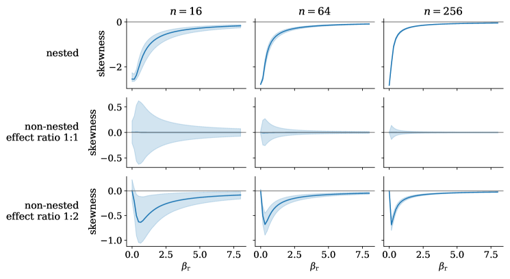
Figure 3: The skewness conditional on the design matrix $X$ for the error ${\mathrm{err}_{\mathrm{\scriptscriptstyle LOO}}\bigr{(}{\mathrm{M}_{a},\mathrm{M}_{b}}\mid y\bigl{)}}$ as a function of a scaling factor $\beta_{\mathrm{r}}\in\mathbb{R}$ for the magnitude of the non-shared effects: $\beta_{\Delta}=\beta_{\mathrm{r}}\beta_{\text{rate}}$. Models have an intercept and one shared covariate. Top: the model ${\mathrm{M}_{b}}$ has one additional covariate. Middle: models ${\mathrm{M}_{a}}$ and ${\mathrm{M}_{b}}$ each have one additional covariate with equal effects. Bottom: models ${\mathrm{M}_{a}}$ and ${\mathrm{M}_{b}}$ have one additional covariate with an effect ratio of 1:2. The solid lines correspond to the median, and the shaded area illustrates the 95 % interval based on 2000 simulated $X$s. The problematic skewness occurs, particularly with the nested models (top row) when $\beta_{r}$ is close to 0 so that the models are making similar predictions (Scenario 1). In the non-nested case, the extreme skewness decreases when $n$ grows, more noticeably in the case of equal effects, but in the nested case, the extreme skewness stays high when $n$ grows.

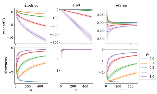
Figure 4: The mean relative to the standard deviation and skewness conditional on the design matrix $X$ for ${\widehat{\mathrm{elpd}}_{\mathrm{\scriptscriptstyle LOO}}\bigr{(}{\mathrm{M}_{a},\mathrm{M}_{b}}\mid y\bigl{)}}$, ${\mathrm{elpd}\bigr{(}{\mathrm{M}_{a},\mathrm{M}_{b}}\mid y\bigl{)}}$, and for the error ${\mathrm{err}_{\mathrm{\scriptscriptstyle LOO}}\bigr{(}{\mathrm{M}_{a},\mathrm{M}_{b}}\mid y\bigl{)}}$ as a function of the data size $n$. The relative mean serves as an indicator of how far away the distribution is from 0. The true model has an intercept and two covariates. One of the covariates with true effect $\beta_{\Delta}$ is included only in model ${\mathrm{M}_{b}}$. The solid lines correspond to the median, and the shaded area illustrates the 95% interval based on 2000 simulated $X$s. The problematic skewness of the error occurs with small $n$ and $\beta_{\Delta}$. When $\beta_{\Delta}=0$, the magnitude of skewness does no decrease when $n$ grows. The relative mean of the error approaches zero when $n$ grows.

Outliers

Outliers in the data impact the moments of the distribution of the error ${\mathrm{err}_{\mathrm{\scriptscriptstyle LOO}}\bigr{(}{\mathrm{M}_{a},\mathrm{M}_{b}}\mid y\bigl{)}}$ in a fickle way. Depending on the data $X$, covariate effect vector $\beta$, and on the outlier design vector $\mu_{\star}$, scaling the outliers can affect the bias of the error quadratically, linearly or not at all. The variance is affected quadratically or not at all. If the scaling affects the variance, the skewness asymptotically converges to zero. We summarise this results in the following proposition.

Proposition 5

Consider mean the $m_{1}$, the variance $\overline{m}_{2}$, and the third central moment $\overline{m}_{3}$ for the variable ${\mathrm{err}_{\mathrm{\scriptscriptstyle LOO}}\bigr{(}{\mathrm{M}_{a},\mathrm{M}_{b}}\mid y\bigl{)}}$. Let $\mu_{\star}=\mu_{\star,\mathrm{r}}\mu_{\star,\text{rate}}+\mu_{\star,\text{base}}$, where $\mu_{\star,\mathrm{r}}\in\mathbb{R}$, $\mu_{\star,\text{rate}}\in\mathbb{R}^{n}\setminus\{0\}$, and $\mu_{\star,\text{base}}\in\mathbb{R}^{n}$. Now $m_{1}$ is a second or first degree polynomial or constant as a function of $\mu_{\star,\mathrm{r}}$. Furthermore, $\overline{m}_{2}$ and $\overline{m}_{3}$ are either both second degree polynomials or both constants and thus, if not constant, the skewness

$$\lim_{\mu_{\star,\mathrm{r}}\rightarrow\pm\infty}\widetilde{m}_{3}=\lim_{\mu_{\star,r}\rightarrow\pm\infty}\frac{\overline{m}_{3}}{(\overline{m}_{2})^{3/2}}=0\,.$$ (19)

Proof  See Appendix D.5.3.
As demonstrated in Figure 5, while the skewness decreases, the relative bias increases and the approximation gets increasingly bad. When $\mu_{\star}\neq 0$, the problematic skewness of the error ${\mathrm{err}_{\mathrm{\scriptscriptstyle LOO}}\bigr{(}{\mathrm{M}_{a},\mathrm{M}_{b}}\mid y\bigl{)}}$ may occur with any level of non-shared covariate effects $\beta_{\Delta}$. This behaviour is shown in Appendix D.6.3.

Residual Variance

The skewness of the error ${\mathrm{err}_{\mathrm{\scriptscriptstyle LOO}}\bigr{(}{\mathrm{M}_{a},\mathrm{M}_{b}}\mid y\bigl{)}}$ converges to a constant value when the true residual variance grows. When the observations are uncorrelated, and they have the same residual variance so that $\Sigma_{\star}=\sigma_{\star}^{2}\mathrm{I}$, the skewness converges to a constant, determined by the design matrix $X$ when $\sigma_{\star}^{2}\rightarrow\infty$. We summarise this behaviour in the following proposition.

Proposition 6

For the data generating process defined in Equation (11), let $\Sigma_{\star}=\sigma_{\star}^{2}\mathrm{I}_{n}$, and Consider the skewness $\widetilde{m}_{3}$ for the variable ${\mathrm{err}_{\mathrm{\scriptscriptstyle LOO}}\bigr{(}{\mathrm{M}_{a},\mathrm{M}_{b}}\mid y\bigl{)}}$. Then,

$$\lim_{\sigma_{\star}\rightarrow\infty}\widetilde{m}_{3}=2^{3/2}\frac{\operatorname{tr}\mathopen{}\mathclose{{}\left(A_{\mathrm{err}}^{3}}\right)}{\operatorname{tr}\mathopen{}\mathclose{{}\left(A_{\mathrm{err}}^{2}}\right)^{3/2}}\,.$$ (20)

Proof  See Appendix D.5.4.

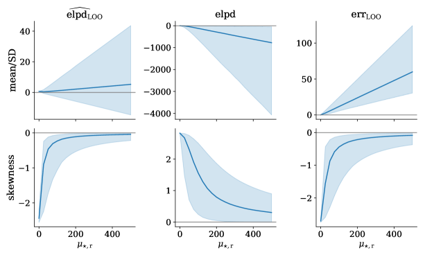
Figure 5: Illustration of the mean relative to the standard deviation and skewness conditional on the design matrix $X$ for ${\widehat{\mathrm{elpd}}_{\mathrm{\scriptscriptstyle LOO}}\bigr{(}{\mathrm{M}_{a},\mathrm{M}_{b}}\mid y\bigl{)}}$, ${\mathrm{elpd}\bigr{(}{\mathrm{M}_{a},\mathrm{M}_{b}}\mid y\bigl{)}}$, and for the error ${\mathrm{err}_{\mathrm{\scriptscriptstyle LOO}}\bigr{(}{\mathrm{M}_{a},\mathrm{M}_{b}}\mid y\bigl{)}}$ as a function of a scaling factor $\mu_{\star,\mathrm{r}}$ for the magnitude of one outlier observation. The data consist of an intercept and two covariates, one of which has no effect and is considered only in the model ${\mathrm{M}_{b}}$. The illustrated behaviour is similar also for other levels of effect for the non-shared covariate. The solid lines correspond to the median, and the shaded area illustrates the 95 % confidence interval based on 2000 independently simulated $X$s from the standard normal distribution. The skewness of all the inspected variables approaches zero when $n$ grows. However, at the same time, the bias of the estimator increases, thus making the analysis of the uncertainty hard.

3.4 Asymptotic Behaviour as a Function of the Data Size

Following the setting defined in (11) and (12), by inspecting the moments in an example case, where a null model is compared to a model with one covariate, we can further draw some interesting conclusions about the behaviour of the moments when $n\rightarrow\infty$, namely:

Proposition 7

Let the setting be defined as in (11) and (12). In addition, let $\beta_{\Delta}\in\mathbb{R}$ be the true effect of the sole non-shared covariate that controls the similarity of the model performances, $\tau^{2}$ is the model variance, and $\Sigma_{\star}=s_{\star}^{2}\mathrm{I}$ is the true residual variance, then

$$\lim_{n\rightarrow\infty}\frac{\operatorname{E}\mathopen{}\mathclose{{}\left[{\widehat{\mathrm{elpd}}_{\mathrm{\scriptscriptstyle LOO}}\bigr{(}{\mathrm{M}_{a},\mathrm{M}_{b}}\mid y\bigl{)}}}\right]}{\operatorname{SD}\mathopen{}\mathclose{{}\left[{\widehat{\mathrm{elpd}}_{\mathrm{\scriptscriptstyle LOO}}\bigr{(}{\mathrm{M}_{a},\mathrm{M}_{b}}\mid y\bigl{)}}}\right]} =\begin{dcases}\frac{\tau^{2}}{\sqrt{2}s_{\star}^{2}}\,,&\text{when }\beta_{\Delta}=0\,,\\ -\infty&\text{otherwise,}\end{dcases}$$ (21)

$$\lim_{n\rightarrow\infty}\frac{\operatorname{E}\mathopen{}\mathclose{{}\left[{\mathrm{elpd}\bigr{(}{\mathrm{M}_{a},\mathrm{M}_{b}}\mid y\bigl{)}}}\right]}{\operatorname{SD}\mathopen{}\mathclose{{}\left[{\mathrm{elpd}\bigr{(}{\mathrm{M}_{a},\mathrm{M}_{b}}\mid y\bigl{)}}}\right]} =\begin{dcases}\frac{\tau^{2}}{\sqrt{2}s_{\star}^{2}}\,,&\text{when }\beta_{\Delta}=0\,,\\ -\infty&\text{otherwise,}\end{dcases}$$ (22)

$$\lim_{n\rightarrow\infty}\frac{\operatorname{E}\mathopen{}\mathclose{{}\left[{\mathrm{err}_{\mathrm{\scriptscriptstyle LOO}}\bigr{(}{\mathrm{M}_{a},\mathrm{M}_{b}}\mid y\bigl{)}}}\right]}{\operatorname{SD}\mathopen{}\mathclose{{}\left[{\mathrm{err}_{\mathrm{\scriptscriptstyle LOO}}\bigr{(}{\mathrm{M_{A},M_{B}}}\mid y\bigl{)}}}\right]} =0$$ (23)

$$\lim_{n\rightarrow\infty}\operatorname{skewness}\mathopen{}\mathclose{{}\left[{\mathrm{err}_{\mathrm{\scriptscriptstyle LOO}}\bigr{(}{\mathrm{M}_{a},\mathrm{M}_{b}}\mid y\bigl{)}}}\right] =\begin{dcases}-2^{3/2},&\text{when }\beta_{\Delta}=0\\ 0&\text{otherwise,}\end{dcases}$$ (24)

Proof  See Appendices D.6.1,  D.6.2,  D.6.3, and D.6.3.
When $\beta_{\Delta}=0$, the relative means of both ${\mathrm{elpd}}$ and ${\widehat{\mathrm{elpd}}_{\mathrm{\scriptscriptstyle LOO}}}$ converge to the same non-zero value, that is the simpler, more parsimonious model performs better asymptotically. As a comparison, in the non-Bayesian linear regression setting with squared error inspected by Shao (1993), both models have asymptotically equal predictive performance with all $y$. Similarly, when $\beta_{\Delta}=0$, the skewness of the error converges to a non-zero value, which indicates that analysing the uncertainty will be problematic also with big data for models with very similar predictive performance (Scenario 1).

Even though we do not expect an underlying effect of a non-shared covariate to be precisely zero in practice, the analysed moments may still behave similarly even with large data size when the effect size is small enough. When $\beta_{\Delta}\neq 0$, the relative mean of both $|{\mathrm{elpd}}|$ and $|{\widehat{\mathrm{elpd}}_{\mathrm{\scriptscriptstyle LOO}}}|$ grows infinitely, and the skewness of the error converges to zero; the more complex model performs better in general, and the problematic skewness hinders when more data is available. The relative mean of error converges to zero, regardless of $\beta_{\Delta}$. Hence, the approximation bias decreases with more data in any case. The example case and the behaviour of the moments are presented in more detail in Appendix D.6. While describing the behaviour in an example case, as demonstrated experimentally in Figure 4, the pattern generalises into other linear regression model comparison settings. Nevertheless, the case analysis shows that a simpler model can outperform a more complex one also asymptotically. In addition, the skewness of the error can be problematic also with big data.

4 Simulation Experiments

In this section, we present results of simulation experiments in which the uncertainty of LOO-CV model comparison is assessed in normal linear regression as in Section 3, but without conditioning on the design matrix $X$ and the model variance $\tau$. Similar to the theoretical analysis in Section 3, we analyse the finite sample properties of the estimator ${\widehat{\mathrm{elpd}}_{\mathrm{\scriptscriptstyle LOO}}\bigr{(}{\mathrm{M}_{a},\mathrm{M}_{b}}\mid y\bigl{)}}$, of the ${\mathrm{elpd}\bigr{(}{\mathrm{M}_{a},\mathrm{M}_{b}}\mid y\bigl{)}}$, and of the error ${\mathrm{err}_{\mathrm{\scriptscriptstyle LOO}}\bigr{(}{\mathrm{M}_{a},\mathrm{M}_{b}}\mid y\bigl{)}}$ for the similarity of model performances (Scenario 1), model misspecification through the effect of an outlier observation (Scenario 2), and the effect of the sample size $n$ (Scenario 3). We also inspect the calibration of the uncertainty estimates. The source code for the experiments is available at https://github.com/avehtari/loocv_uncertainty.

4.1 Experiment Settings

We compare two nested linear regression models under data simulated from a linear regression model being $p_{\text{true}}(y)$. The data generating mechanism follows the definition in (11), where $d=3$, $X_{i}=[1,X_{[i,2]},X_{[i,3]}]$, $X_{[i,1]},X_{[i,2]}\sim\operatorname{N}(0,1)$ for $i=1,2,\dots,n$, $\beta=[0,1,\beta_{\Delta}]$, $\mu_{\star}=[\mu_{\star,0},0,\dots,0]$, and, $\Sigma_{\star}=\mathrm{I}$. The models $\mathrm{M}_{a}$ and $\mathrm{M}_{b}$ follow the definition in (12) with the difference that the residual variance $\tau^{2}$ is now unknown. The model $\mathrm{M}_{a}$ only includes intercept and one covariate, while the model $\mathrm{M}_{b}$ includes one additional covariate with true effect $\beta_{\Delta}$. The similarity of the models is varied with $\beta_{\Delta}$. The data size $n$ varies from $16$ to $1024$. Parameter $\mu_{\star,0}$ is used to scale the mean of one observation so that, when large enough, that observation becomes an outlier and the models become misspecified. Unless otherwise noted, $\mu_{\star,0}=0$.

We generate $j=1,2,\dots,2000$ data sets from $p_{\text{true}}(y)$, and for each trial $j$, we obtain pointwise LOO-CV estimates ${\widehat{\mathrm{elpd}}_{\mathrm{\scriptscriptstyle LOO},\,i}\bigr{(}{\mathrm{M}_{a}}\mid y\bigl{)}}$ and ${\widehat{\mathrm{elpd}}_{\mathrm{\scriptscriptstyle LOO},\,i}\bigr{(}{\mathrm{M}_{b}}\mid y\bigl{)}}$, which are used to form estimates ${\widehat{\mathrm{elpd}}_{\mathrm{\scriptscriptstyle LOO}}\bigr{(}{\mathrm{M}_{a},\mathrm{M}_{b}}\mid y\bigl{)}}$ and ${\widehat{\mathrm{SE}}_{\mathrm{\scriptscriptstyle LOO}}\bigr{(}{\mathrm{M}_{a},\mathrm{M}_{b}}\mid y\bigl{)}}$ in particular. The respective target values ${\mathrm{elpd}\bigr{(}{\mathrm{M}_{a}}\mid y\bigl{)}}$ and ${\mathrm{elpd}\bigr{(}{\mathrm{M}_{b}}\mid y\bigl{)}}$ are obtained using an independent test set of 4000 data sets of the same size simulated from the same data generating mechanism.

4.2 Behaviour of the Sampling and the Error Distribution

The moments of the sampling distribution of ${\widehat{\mathrm{elpd}}_{\mathrm{\scriptscriptstyle LOO}}\bigr{(}{\mathrm{M}_{a},\mathrm{M}_{b}}\mid y\bigl{)}}$, the distribution of the ${\mathrm{elpd}\bigr{(}{\mathrm{M}_{a},\mathrm{M}_{b}}\mid y\bigl{)}}$, and the error distribution ${\mathrm{err}_{\mathrm{\scriptscriptstyle LOO}}\bigr{(}{\mathrm{M}_{a},\mathrm{M}_{b}}\mid y\bigl{)}}$ behave similarly in these simulated experiments and in the theoretical analysis conditional on the design matrix $X$ and known model variance $\tau$ (Section 3). In particular, when $\beta_{\Delta}=0$ and $n$ grow, LOO-CV is slightly more likely to pick the simpler model with a constant difference in the predictive performance, and the magnitude of the skewness does not fade away. With this experiment setting, however, the skewness of ${\mathrm{elpd}\bigr{(}{\mathrm{M}_{a},\mathrm{M}_{b}}\mid y\bigl{)}}$ decreases when $\beta_{\Delta}$ grows, while in the experiments in Section 3, this skewness is similar with all $\beta_{\Delta}$. Figure 12 in Appendix E illustrates the behaviour of the moments in more detail.

4.3 Negative Correlation and Bias

Figure 6 illustrates the joint distribution of ${\widehat{\mathrm{elpd}}_{\mathrm{\scriptscriptstyle LOO}}\bigr{(}{\mathrm{M}_{a},\mathrm{M}_{b}}\mid y\bigl{)}}$ and ${\mathrm{elpd}\bigr{(}{\mathrm{M}_{a},\mathrm{M}_{b}}\mid y\bigl{)}}$ for various non-shared covariate effects $\beta_{\Delta}$ and data sizes $n$. The estimator and ${\mathrm{elpd}\bigr{(}{\mathrm{M}_{a},\mathrm{M}_{b}}\mid y\bigl{)}}$ get negatively correlated when the model performances get more similar (Scenario 1). The effect is more noticeable with larger $n$. Similar to Figure 6, Figure 14 in Appendix E illustrates the joint distribution of ${\widehat{\mathrm{elpd}}_{\mathrm{\scriptscriptstyle LOO}}\bigr{(}{\mathrm{M}_{a},\mathrm{M}_{b}}\mid y\bigl{)}}$ and ${\mathrm{elpd}\bigr{(}{\mathrm{M}_{a},\mathrm{M}_{b}}\mid y\bigl{)}}$ when there is an outlier observation in the data set (Scenario 2).

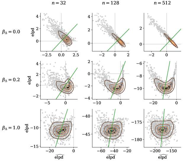
Figure 6: Illustration of the joint distribution of ${\widehat{\mathrm{elpd}}_{\mathrm{\scriptscriptstyle LOO}}\bigr{(}{\mathrm{M}_{a},\mathrm{M}_{b}}\mid y\bigl{)}}$ and ${\mathrm{elpd}\bigr{(}{\mathrm{M}_{a},\mathrm{M}_{b}}\mid y\bigl{)}}$ for various data sizes $n$ and non-shared covariate effects $\beta_{\Delta}$. The green diagonal line indicates where the variables match. The problematic negative correlation occurs when $\beta_{\Delta}=0$. In addition, while decreasing in correlation, the nonlinear dependency in the transition from small to large $\beta_{\Delta}$ is problematic.

Figures 15 and  16 in Appendix E show that when there are an outlier present in the data, the relative error’s mean usually clearly deviates from zero, and the estimator is biased.

4.4 Behaviour of the Uncertainty Estimates

Due to the mismatch between the forms of the sampling and the error distribution, estimated uncertainties based on the sampling distribution can be poorly calibrated. The problem of underestimating the variance is illustrated in Figures 19 and 20 in Appendix E. Figure 7 illustrates the calibration of the estimated uncertainties in different setings.

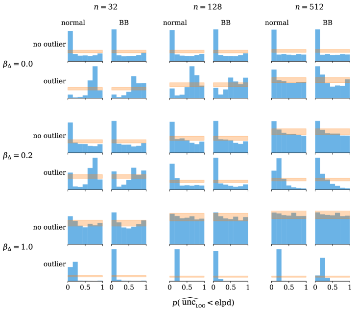
Figure 7: Calibration of the estimated uncertainty $p({\mathrm{elpd}\bigr{(}{\mathrm{M}_{a},\mathrm{M}_{b}}\mid y\bigl{)}})$ for various data sizes $n$ and non-shared covariate effects $\beta_{\Delta}$. The histograms illustrate the PIT values $q\Bigl{(}{\mathrm{elpd}\bigr{(}{\mathrm{M}_{a},\mathrm{M}_{b}}\mid y\bigl{)}}<{\widehat{\mathrm{elpd}}_{\mathrm{\scriptscriptstyle LOO}}\bigr{(}{\mathrm{M}_{a},\mathrm{M}_{b}}\mid y\bigl{)}}\Bigr{)}$ over simulated data sets $y$, which would be uniform in a case of optimal calibration (see e.g. Gneiting et al., 2007; Säilynoja et al., 2021). The yellow shading indicates the range of 99 % of the variation expected from uniformity. Two uncertainty estimators are presented: normal approximation and BB. in case of outlier, that observation has a deviated mean of 20 times the standard deviation of $y_{i}$. The calibration is better when $\beta_{\Delta}$ is large or $n$ is big. The outlier makes the calibration worse, although with large $n$ and small $\beta_{\Delta}$, the calibration can be better, as outlier inflates the variance.

Normal and BB approximation produce similar results. A small sample size (Scenario 3) and similarity in the predictive performance between the models (Scenario 1) can cause problems. Similarly, model misspecification through an outlier observation (Scenario 2) can make the calibration worse. On the other hand, in the experiment with $n=512$ and $\beta_{\Delta}=0$, the calibration is better with an outlier as the outlier inflates the variance. The skewness of the error has decreased more than the bias has increased. This effect is illustrated in more detail in Figures 5 and 12 in Appendix E.

4.5 Experiments with more model variants

In this section, we present empirical results for six model variants, illustrating that the theoretical results generalise beyond the simplest case. We study models with 2) more covariates, 3) non-Gaussianity, 4) hierarchy, and 5) non-linearity. We also demonstrate the behaviour with 1) fixed covariate values and 6) K-fold-CV. All the additional experiments have two nested regression models with data-generating mechanisms similar to (11), where $d=3$, $\beta=[0,1,\beta_{\Delta}]$, and, $\Sigma_{\star}=\mathrm{I}$. The model $\mathrm{M}_{a}$ is a (generalised) linear model with intercept and one covariate, following the structure as in (12). The model $\mathrm{M}_{b}$ follows the data generating process by including the true covariate. For simplicity, we only present the data generating processes, as the model $\mathrm{M}_{b}$ follows the same structure.

1. A linear model with fixed (non-random) covariate values. The models are the same as in Equation (12), but covariate $X_{2}$ is defined as a fixed uniform sequence $X_{2}=-1+2k/n$, for $k=1,2,\ldots,n$.

2. Linear model with more common covariates.

   $$Y=1+\sum_{k=1}^{5}Z_{k}+\beta_{\Delta}X_{2}+\varepsilon,$$

   where $Z_{k},X_{2}\sim N(0,1)$, $\varepsilon\sim N(0,\tau^{2})$, and $\tau$ unknown.

3. A linear hierarchical model with $k=4$ groups.

   $$Y=1+X_{1}+\beta_{\Delta}\alpha_{j}+\varepsilon,$$

   $$\alpha_{j}\sim N(\alpha_{0},\sigma^{2}),$$

   where $\varepsilon\sim N(0,\tau^{2})$, $\tau$ unknown, $\alpha_{0}\sim N(0,1)$, and $j=1,2,3,k$.

4. A Poisson generalised linear model. $Y\sim\operatorname{Poisson}(\mu)$, where $\mu=exp(1+X_{1}+\beta_{\Delta}X_{2})$, and $X_{1},X_{2}\sim N(0,1)$.

5. A spline model. The data-generating process follows a non-linear model

   $$Y=X_{1}+\beta_{\Delta}X_{2}\cos(X_{2})+\varepsilon,$$

   where, $X_{1},X_{2}\sim N(0,1)$, $\varepsilon\sim N(0,\tau^{2})$, and $\tau$ unknown. The spline model is

   $$M_{b}:Y=\beta_{0}+\beta_{1}X_{1}+\beta_{2}s(X_{2})+\varepsilon,$$

   where $s(X_{2})$ represent the penalised B-spline matrix obtained for the covariate $X_{2}$.

   

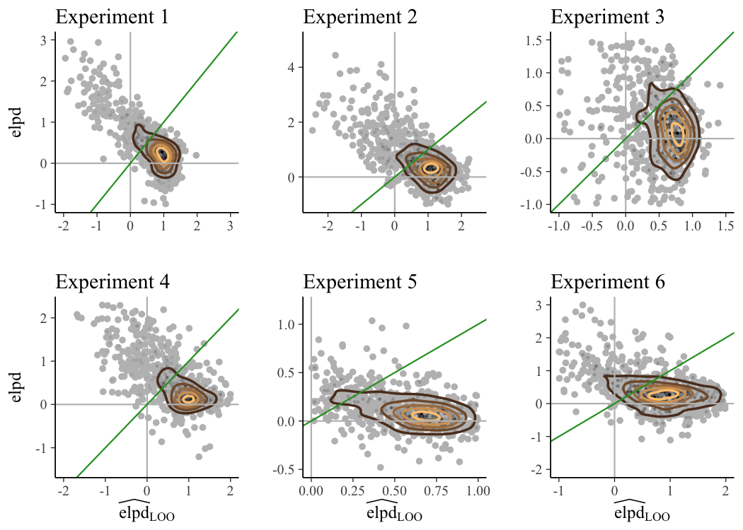
   Figure 8: Illustration of the joint distribution for the LOO-CV estimator and ${\mathrm{elpd}\bigr{(}{\mathrm{M_{A},M_{B}}}\mid y\bigl{)}}$ for sample size of $n=32$, and non-shared covariate effect $\beta_{\Delta}=0.0$. The green diagonal line indicates where the variables match.

6. 10-fold-CV instead of LOO-CV. The model and data are the same as in Section 3, but 10-fold-CV with random complete block design is used. For example, when $K\geq 10$, each observation is left out only once, and the observations left out in each fold are likely not to be neighbours. Thus locally, we get a reasonable approximation of LOO-CV. Globally, as only $n-n/K$ (rounded to an integer) observations are used for the posterior, the predictive performance is likely to be slightly worse than when using $n-1$ observations. We could correct this bias, but this is rarely done, as the bias is often small, and the bias correction increases the variance (Vehtari and Lampinen, 2002). We assume that small bias doesn’t change the general behaviour compared to LOO-CV. If K-fold-CV is used with grouped data division to perform leave-one-group-out cross-validation, the behaviour is much different from LOO-CV, and we leave the analysis for future research.

In every experiment, we generate $1000$ data sets, and for each trial, we obtain pointwise LOO-CV (or 10-fold-CV) estimates ${\widehat{\mathrm{elpd}}_{\mathrm{\scriptscriptstyle LOO}}\bigr{(}{\mathrm{M_{A},M_{B}}}\mid y\bigl{)}}$ and ${\widehat{\mathrm{SE}}_{\mathrm{\scriptscriptstyle LOO}}\bigr{(}{\mathrm{M_{A},M_{B}}}\mid y\bigl{)}}$. The respective target values ${\mathrm{elpd}\bigr{(}{\mathrm{M_{A},M_{B}}}\mid y\bigl{)}}$ are obtained using a separate test set of 4000 data sets of the same size simulated from the same data generating mechanism.

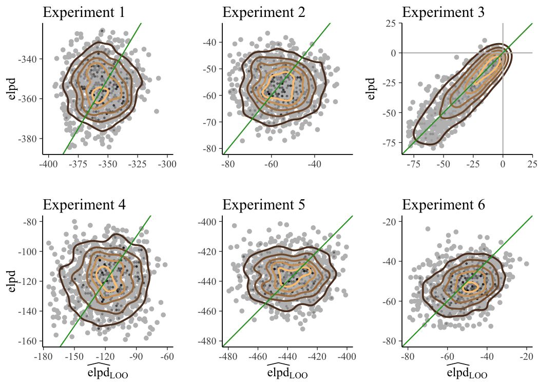
Figure 9: Illustration of the joint distribution for the LOO-CV estimator and ${\mathrm{elpd}\bigr{(}{\mathrm{M_{A},M_{B}}}\mid y\bigl{)}}$ for sample size of $n=512$, and non-shared covariate effect $\beta_{\Delta}=0.5$. The green diagonal line indicates where the variables match.

Figures 8 and 9 illustrate the joint distribution of the LOO-CV estimator and ${\mathrm{elpd}\bigr{(}{\mathrm{M}_{a},\mathrm{M}_{b}}\mid y\bigl{)}}$ for different data sizes $n$ and non-shared covariate effects $\beta_{\Delta}$. Figure 8 shows the results with small $n$ and models with similar predictions ($n=32$ and $\beta_{\Delta}=0$). Figure 9 shows the results with large $n$ and models with different predictions ($n=512$ and $\beta_{\Delta}=0.5$). The results match the theoretical and previous experimental results. In the case of the hierarchical example (Experiment 3), there is a clear positive correlation, as the random realisations of data have variations in how strongly the groups differ, and thus both the estimate and true value have more variation, but the error distribution doesn’t get wider. Additional results are shown in Figures 22 and 23 in Appendix E.

5 Conclusions

LOO-CV is a popular method for estimating the difference in the predictive performance between two models. The associated uncertainty in the estimation is often overlooked. The current popular ways of estimating the uncertainty may lead to poorly calibrated estimations of the uncertainty, underestimating the variability in particular. We discuss two methods of estimating the uncertainty, normal and Bayesian bootstrap approximation, and inspect their properties in Bayesian linear regression. We show that problematic problem settings include models with similar predictions (Scenario 1), model misspecification with outliers in the data (Scenario 2), and small data (Scenario 3).

Scenario 1: Models With Similar Predictions

We show that the problematic skewness of the distribution of the approximation error occurs with models making similar predictions. This skewness does not necessarily disappear as $n$ grows. We show that considering the skewness of the sampling distribution is insufficient to improve the uncertainty estimate, as it has a weak connection to the skewness of the distribution of the estimators’ error. We show that, in the problematic settings, both normal and BB approximations to the uncertainty are badly calibrated.Our analysis shows the properties of the estimator in the linear regression, but we expect the behaviour and the problematic cases to be similar in other typical modeling settings.

Scenario 1 consequences

Given similar predictions we are unlikely to lose much in predictive performance, whichever model is selected. We may get more information about the model differences by looking at the posterior of the model with additional terms.

Scenario 2: Model Misspecification With Outliers

Cross-validation has been advocated for $\mathcal{M}$-open case when the true model is not included in the set of the compared models (Bernardo and Smith, 1994; Vehtari and Ojanen, 2012). Our results demonstrate that there can be significant bias in the estimated predictive performance in the case of bad misspecification, which can affect the model comparison. In this case, analysing the uncertainty of the estimated difference in the predictive performance is difficult.

Scenario 2 consequences

Model checking, and possible refinement, should be considered before using cross-validation for model comparison. The issue of bad model misspecification affecting the model comparison is not unique to cross-validation as demonstrated for Bayes factor, for example, by Oelrich et al. (2020).

Scenario 3: Small Data

Even in the case of well-specified models and models with dissimilar predictions, small data (say $n<100$) makes estimating uncertainty in cross-validation less reliable. When the differences between models are small, or models are slightly misspecified, larger data sets are needed for well-calibrated model comparison.

6 Discussion

This paper is the first to thoroughly study the properties of uncertainty estimates in log-score LOO-CV model comparison in the Bayesian setting. Here, we discuss connections to related methods and useful directions for future research.

Other scoring rules

In this paper, we focused on the log score. We may assume that other smooth, strictly proper scoring rules (Gneiting and Raftery, 2007) would behave similarly. As discussed by Gneiting and Raftery (2007), continuous ranked probability score (CRPS) might be more robust than log score to extreme cases or outliers, but it is unclear how that would affect the uncertainty in the LOO-CV model comparison.

Hierarchical models

As we have on LOO-CV, we used it also for a hierarchical model, which is a valid option when the focus is on analysing the observation model or in predictions for new individuals in the existing groups. For data with a group structure, leave-one-group-out cross-validation can be used to simulate predictions for new groups (see, e.g., Vehtari and Lampinen, 2002; Merkle et al., 2019). If the log score is used to assess the performance of joint predictions for all observations in one group, we get only one log score per group. We may assume that the number of groups is then the decisive factor for the behaviour.If the log score is used to assess the performance of pointwise predictions of observations in a group, the behaviour of is likely to be affected by the ratio of within and between-group variation. With increasing between-group variation, the behaviour approaches the joint prediction case.

Leave-future-out cross-validation

In the case of time series, if the goal is to assess the predictive performance for the future (and not to time points between observations), we can use leave-future-out cross-validation (see, e.g. Bürkner et al., 2020). In this case, the individual log score values are not exchangeable, as the amount of data used to fit the posterior is different for each prediction, and the dependency structure between folds is different. Asymptotically for long time series, this is likely to have a minor effect.

Comparison of multiple models

We focused on comparing two models as analysis of one-dimensional difference distribution is easier. When comparing a few models with LOO-CV, Vehtari et al. (2022a) recommend making pairwise comparisons to the model with the highest log score. This approach reduces the number of comparisons to be one less than the number of models and provides a natural ordering for the comparisons. If the best model is clearly better than others, there is no need to examine the differences and related uncertainties for the rest, and pairwise comparison is sufficient. In case of many models without one clear best model, the model selection induced bias and overfitting can be non-negligible (McLatchie and Vehtari, 2023). In such cases, for variable selection we recommend using projective predictive model selection (Piironen and Vehtari, 2016; Piironen et al., 2020; McLatchie et al., 2023), which has much lower variance than LOO-CV.

Model averaging

If one of the models is not undoubtedly the best, and the aim is the best prediction (no need for model selection) we recommend model averaging. If we stick using LOO-CV based computation, we can follow Yao et al. (2018) and compute model weights using 1) LOO-CV differences, 2) LOO-CV differences plus related uncertainty handled with BB (use of normal approximation gets complicated with many models), or 3) LOO-CV based Bayesian stacking. Yao et al. (2018) show that taking into account the LOO-CV uncertainty improves the LOO weights, but Bayesian stacking performs even better. Both LOO-CV weights have an issue that equal or very similar models get similar weights and dilute the weights of other models, making the interpretation of the weights in model comparison more difficult. On the other hand, Bayesian stacking weights are optimised for predictive model averaging, and the interpretation of weights is also non-trivial (see discussion and examples in Yao et al., 2021).

Acknowledgments

We thank Daniel Simpson and anonymous reviewers for helpful comments and feedback. We acknowledge the computational resources provided by the Aalto Science-IT project. This work was supported by the Academy of Finland grants (298742 and 313122) and Academy of Finland Flagship programme: Finnish Center for Artificial Intelligence FCAI.

Appendices

The included appendices A–E provide supportive discussion and further theoretical and empirical results. Appendices A and B supports Section 2 by studying the differences in the uncertainty when estimating either ${\mathrm{elpd}}$ or e-elpd, and by further discussing the formulation of the uncertainty. Appendix C analyses the behaviour of the normal and BB approximation to the uncertainty in a general setting in more detail. Appendix D presents detailed derivations of the results presented in the theoretical case study in Section 3 and further introduces some more detailed properties. Finally, Appendix E presents some additional empirical results of the simulated experiment presented in Section 4. The notation in the appendices mostly follows the notation used in the main part of the work. However, bold symbols are used to denote vectors and matrices in order to make it easier to distinguish them from scalar variables.

Appendix A Difference Between Estimating elpd and e-elpd

As discussed in the beginning of Section 2, depending on if the context of the model comparison is in evaluating the models for the given data set or for the data generating mechanism in general, the measure of interest is either

$${\mathrm{elpd}\bigr{(}{\mathrm{M}_{k}}\mid y\bigl{)}} =\sum_{i=1}^{n}\int p_{\text{true}}(y_{i})\log p_{k}(y_{i}\mid y)\mathop{}\kern-2.0pt\mathrm{d}y_{i}$$ (25)

or its expectation over possible data sets

$${\text{e-elpd}\bigr{(}{\mathrm{M}_{k}}\bigl{)}} =\operatorname{E}_{y}\mathopen{}\mathclose{{}\left[{\mathrm{elpd}\bigr{(}{\mathrm{M}_{k}}\mid y\bigl{)}}}\right]$$ (26)

respectively. The uncertainty related to the ${\widehat{\mathrm{elpd}}_{\mathrm{\scriptscriptstyle LOO}}}$ estimator is different depending on if it is used to estimate ${\mathrm{elpd}\bigr{(}{\mathrm{M}_{a},\mathrm{M}_{b}}\mid y\bigl{)}}$ or ${\text{e-elpd}\bigr{(}{\mathrm{M}_{a},\mathrm{M}_{b}}\bigl{)}}$. While otherwise focusing on analysing the nature of the uncertainty in the application-oriented context of ${\mathrm{elpd}\bigr{(}{\mathrm{M}_{a},\mathrm{M}_{b}}\mid y\bigl{)}}$ measure,in this appendix we formulate the uncertainties related to both measures and discuss their differences in more detail. The following analysis of the uncertainty generalises also for estimating ${\text{e-elpd}\bigr{(}{\mathrm{M}_{k}}\bigl{)}}$ or ${\mathrm{elpd}\bigr{(}{\mathrm{M}_{k}}\mid y\bigl{)}}$ for one model and for other $K$-fold CV estimators.

A.1 Estimating e-elpd

When using ${\widehat{\mathrm{elpd}}_{\mathrm{\scriptscriptstyle LOO}}\bigr{(}{\mathrm{M}_{a},\mathrm{M}_{b}}\mid y\bigl{)}}$ to estimate ${\text{e-elpd}\bigr{(}{\mathrm{M}_{a},\mathrm{M}_{b}}\bigl{)}}$, ${\widehat{\mathrm{elpd}}_{\mathrm{\scriptscriptstyle LOO}}\bigr{(}{\mathrm{M}_{a},\mathrm{M}_{b}}\mid y\bigl{)}}$ is an estimator considering $(y)$ as a random sample of the stochastic variable $y$. Any observed data set $y$ can be used to estimate the same quantity ${\text{e-elpd}\bigr{(}{\mathrm{M}_{a},\mathrm{M}_{b}}\bigl{)}}$. The uncertainty about the ${\text{e-elpd}\bigr{(}{\mathrm{M}_{a},\mathrm{M}_{b}}\bigl{)}}$ given an estimate can be assessed by considering the error over possible data sets,

$${\mathrm{err}_{\mathrm{\scriptscriptstyle LOO}}^{{\text{e-elpd}}}\bigr{(}{\mathrm{M}_{a},\mathrm{M}_{b}}\mid y\bigl{)}}={\widehat{\mathrm{elpd}}_{\mathrm{\scriptscriptstyle LOO}}\bigr{(}{\mathrm{M}_{a},\mathrm{M}_{b}}\mid y\bigl{)}}-{\text{e-elpd}\bigr{(}{\mathrm{M}_{a},\mathrm{M}_{b}}\bigl{)}}\,,$$ (27)

which corresponds to the estimator’s sampling distribution ${\widehat{\mathrm{elpd}}_{\mathrm{\scriptscriptstyle LOO}}\bigr{(}{\mathrm{M}_{a},\mathrm{M}_{b}}\mid y\bigl{)}}$ shifted by a constant.

A.2 Estimating elpd

When using ${\widehat{\mathrm{elpd}}_{\mathrm{\scriptscriptstyle LOO}}\bigr{(}{\mathrm{M}_{a},\mathrm{M}_{b}}\mid y\bigl{)}}$ to approximate ${\mathrm{elpd}\bigr{(}{\mathrm{M}_{a},\mathrm{M}_{b}}\mid y\bigl{)}}$, however, $y$ is given also in the approximated quantity. Each observed data set $y$ can be used to approximate different quantity ${\mathrm{elpd}\bigr{(}{\mathrm{M}_{a},\mathrm{M}_{b}}\mid y\bigl{)}}$. Here the error is formulated as

$${\mathrm{err}_{\mathrm{\scriptscriptstyle LOO}}^{{\mathrm{elpd}}}\bigr{(}{\mathrm{M}_{a},\mathrm{M}_{b}}\mid y\bigl{)}}={\widehat{\mathrm{elpd}}_{\mathrm{\scriptscriptstyle LOO}}\bigr{(}{\mathrm{M}_{a},\mathrm{M}_{b}}\mid y\bigl{)}}-{\mathrm{elpd}\bigr{(}{\mathrm{M}_{a},\mathrm{M}_{b}}\mid y\bigl{)}}\,.$$ (28)

Even though reflecting a different problem for each realisation of the data set, the associated uncertainty about one problem can be assessed by analysing the approximation error over possible data sets is in a similar fashion as when estimating ${\text{e-elpd}\bigr{(}{\mathrm{M}_{a},\mathrm{M}_{b}}\bigl{)}}$. However, here the variability of ${\mathrm{err}_{\mathrm{\scriptscriptstyle LOO}}\bigr{(}{\mathrm{M}_{a},\mathrm{M}_{b}}\mid y\bigl{)}}$ depends both on ${\widehat{\mathrm{elpd}}_{\mathrm{\scriptscriptstyle LOO}}\bigr{(}{\mathrm{M}_{a},\mathrm{M}_{b}}\mid y\bigl{)}}$ and ${\mathrm{elpd}\bigr{(}{\mathrm{M}_{a},\mathrm{M}_{b}}\mid y\bigl{)}}$.

A.3 Error Distributions

Assuming the observations $y_{i}$, $i=1,2,\dots,n$ are independent, the expectation of the error distributions for both measures ${\mathrm{elpd}}$ and e-elpd are the same, that is

$$\operatorname{E}\mathopen{}\mathclose{{}\left[{\mathrm{err}_{\mathrm{\scriptscriptstyle LOO}}^{{\mathrm{elpd}}}\bigr{(}{\mathrm{M}_{a},\mathrm{M}_{b}}\mid y\bigl{)}}}\right] =\operatorname{E}\mathopen{}\mathclose{{}\left[{\mathrm{err}_{\mathrm{\scriptscriptstyle LOO}}^{{\text{e-elpd}}}\bigr{(}{\mathrm{M}_{a},\mathrm{M}_{b}}\mid y\bigl{)}}}\right]\,,$$ (29)

but they differ in variability. In particular, as demonstrated for example in Figure 1, the correlation of ${\widehat{\mathrm{elpd}}_{\mathrm{\scriptscriptstyle LOO}}\bigr{(}{\mathrm{M}_{a},\mathrm{M}_{b}}\mid y\bigl{)}}$ and ${\mathrm{elpd}\bigr{(}{\mathrm{M}_{a},\mathrm{M}_{b}}\mid y\bigl{)}}$ is generally small or negative and thus the variance,

$$\operatorname{Var}\mathopen{}\mathclose{{}\left({\mathrm{err}_{\mathrm{\scriptscriptstyle LOO}}^{{\mathrm{elpd}}}\bigr{(}{\mathrm{M}_{a},\mathrm{M}_{b}}\mid y\bigl{)}}}\right) =\operatorname{Var}\mathopen{}\mathclose{{}\left({\widehat{\mathrm{elpd}}_{\mathrm{\scriptscriptstyle LOO}}\bigr{(}{\mathrm{M}_{a},\mathrm{M}_{b}}\mid y\bigl{)}}}\right)+\operatorname{Var}\mathopen{}\mathclose{{}\left({\mathrm{elpd}\bigr{(}{\mathrm{M}_{a},\mathrm{M}_{b}}\mid y\bigl{)}}}\right)$$

$$\quad-2\operatorname{Cov}\mathopen{}\mathclose{{}\left({\widehat{\mathrm{elpd}}_{\mathrm{\scriptscriptstyle LOO}}\bigr{(}{\mathrm{M}_{a},\mathrm{M}_{b}}\mid y\bigl{)}},{\mathrm{elpd}\bigr{(}{\mathrm{M}_{a},\mathrm{M}_{b}}\mid y\bigl{)}}}\right)$$ (30)

is usually greater than

$$\operatorname{Var}\mathopen{}\mathclose{{}\left({\mathrm{err}_{\mathrm{\scriptscriptstyle LOO}}^{{\text{e-elpd}}}\bigr{(}{\mathrm{M}_{a},\mathrm{M}_{b}}\mid y\bigl{)}}}\right) =\operatorname{Var}\mathopen{}\mathclose{{}\left({\widehat{\mathrm{elpd}}_{\mathrm{\scriptscriptstyle LOO}}\bigr{(}{\mathrm{M}_{a},\mathrm{M}_{b}}\mid y\bigl{)}}}\right)\,.$$ (31)

Because of the differences in the error distributions, it is significant to consider the uncertainties separately for both measures ${\mathrm{elpd}}$ and e-elpd.

A.4 Sampling Distributions

When estimating ${\text{e-elpd}\bigr{(}{\mathrm{M}_{a},\mathrm{M}_{b}}\bigl{)}}$, ${\widehat{\mathrm{elpd}}_{\mathrm{\scriptscriptstyle LOO}}\bigr{(}{\mathrm{M}_{a},\mathrm{M}_{b}}\mid y\bigl{)}}$ is a random variable corresponding to the estimator’s sampling distribution for the specific problem. However, when approximating ${\mathrm{elpd}\bigr{(}{\mathrm{M}_{a},\mathrm{M}_{b}}\mid y\bigl{)}}$, ${\widehat{\mathrm{elpd}}_{\mathrm{\scriptscriptstyle LOO}}\bigr{(}{\mathrm{M}_{a},\mathrm{M}_{b}}\mid y\bigl{)}}$ and ${\mathrm{err}_{\mathrm{\scriptscriptstyle LOO}}^{{\mathrm{elpd}}}\bigr{(}{\mathrm{M}_{a},\mathrm{M}_{b}}\mid y\bigl{)}}$ are stochastic variables reflecting the frequency properties of the approximation when applied for different problems. Nevertheless, we refer to ${\widehat{\mathrm{elpd}}_{\mathrm{\scriptscriptstyle LOO}}\bigr{(}{\mathrm{M}_{a},\mathrm{M}_{b}}\mid y\bigl{)}}$ as an estimator and ${\widehat{\mathrm{elpd}}_{\mathrm{\scriptscriptstyle LOO}}\bigr{(}{\mathrm{M}_{a},\mathrm{M}_{b}}\mid y\bigl{)}}$ as a sampling distribution also in the latter context. Note however that other assessments of the uncertainty of the estimator $\widehat{\mathrm{elpd}}_{\mathrm{\scriptscriptstyle LOO}}$ for ${\mathrm{elpd}\bigr{(}{\mathrm{M}_{a},\mathrm{M}_{b}}\mid y\bigl{)}}$ can be made. The related formulation of the target uncertainty about ${\mathrm{elpd}\bigr{(}{\mathrm{M}_{a},\mathrm{M}_{b}}\mid y\bigl{)}}$ is discussed in more detail in Appendix B.

Appendix B Alternative Formulations of the Uncertainty

In Appendix A, we analyse and motivate the method applied in the paper and mention that other approaches can be made for assessing the uncertainty about ${\mathrm{elpd}\bigr{(}{\mathrm{M}_{a},\mathrm{M}_{b}}\mid y\bigl{)}}$. In this appendix we discuss some of these and further motivate the applied method. Instead of analysing the error stochastically over possible data sets, it is also possible, for example, to find bounds or apply Bayesian inference for the error. As briefly discussed in Section 2.2, also other formulations of the target uncertainty

$${\mathrm{unc}_{\mathrm{\scriptscriptstyle LOO}}\bigr{(}{\mathrm{M}_{a},\mathrm{M}_{b}}\mid y\bigl{)}}={\widehat{\mathrm{elpd}}_{\mathrm{\scriptscriptstyle LOO}}\bigr{(}{\mathrm{M}_{a},\mathrm{M}_{b}}\mid y\bigl{)}}-{\mathrm{err}_{\mathrm{\scriptscriptstyle LOO}}\bigr{(}{\mathrm{M}_{a},\mathrm{M}_{b}}\mid y\bigl{)}},$$ (32)

may satisfy the desired equality

$$q\Bigr{(}{\mathrm{unc}_{\mathrm{\scriptscriptstyle LOO}}\bigr{(}{\mathrm{M}_{a},\mathrm{M}_{b}}\mid y\bigl{)}}\Bigl{)}=p\Bigr{(}{\mathrm{elpd}\bigr{(}{\mathrm{M}_{a},\mathrm{M}_{b}}\mid y\bigl{)}}\Bigl{)}\,.$$ (33)

For example, while not sensible as a target for the estimated uncertainty, assigning Dirac delta function located at ${\mathrm{elpd}\bigr{(}{\mathrm{M}_{a},\mathrm{M}_{b}}\mid y\bigl{)}}$ as a probability distribution for ${\mathrm{unc}_{\mathrm{\scriptscriptstyle LOO}}\bigr{(}{\mathrm{M}_{a},\mathrm{M}_{b}}\mid y\bigl{)}}$ trivially satisfies Equation (33). Some other approach, however, might also provide feasible uncertainty estimator target. In particular, these alternative formulations could be developed for specific problem setting.

B.1 LOO-CV Estimate With Independent Test Data

One possible general interpretation of the uncertainty could arise by considering ${\widehat{\mathrm{elpd}}_{\mathrm{\scriptscriptstyle LOO}}}$ as one possible realised estimation from the following estimator. Let

$${\widehat{\mathrm{elpd}}_{\mathrm{\scriptscriptstyle LOO}}\bigr{(}{\mathrm{M}_{k}}\mid\tilde{y}^{\mathrm{obs}},y\bigl{)}} =\sum_{i=1}^{n}\log p_{k}\mathopen{}\mathclose{{}\left(\tilde{y}^{\mathrm{obs}}_{i}\mid y_{-i}}\right)\,.$$ (34)

In this estimator, the data set $\tilde{y}^{\mathrm{obs}}$ is considered a random sample for estimating $p_{\text{true}}(y)$ and $y$ is a given data set indicating the problem at hand in the ${\mathrm{elpd}\bigr{(}{\mathrm{M}_{k}}\mid y\bigl{)}}$, i.e. the training and test data sets are separated. Now ${\widehat{\mathrm{elpd}}_{\mathrm{\scriptscriptstyle LOO}}\bigr{(}{\mathrm{M}_{k}}\mid y\bigl{)}}={\widehat{\mathrm{elpd}}_{\mathrm{\scriptscriptstyle LOO}}\bigr{(}{\mathrm{M}_{k}}\mid y,y\bigl{)}}$ is one application of this estimator, where the same data set is re-used for both arguments. The uncertainty of the estimator ${\widehat{\mathrm{elpd}}_{\mathrm{\scriptscriptstyle LOO}}\bigr{(}{\mathrm{M}_{a},\mathrm{M}_{b}}\mid\tilde{y}^{\mathrm{obs}},y\bigl{)}}$ can be formulated in the following way:

$${\mathrm{unc}_{\mathrm{\scriptscriptstyle LOO}}\bigr{(}{\mathrm{M}_{a},\mathrm{M}_{b}}\mid\tilde{y}^{\mathrm{obs}},y\bigl{)}} ={\widehat{\mathrm{elpd}}_{\mathrm{\scriptscriptstyle LOO}}\bigr{(}{\mathrm{M}_{a},\mathrm{M}_{b}}\mid\tilde{y}^{\mathrm{obs}},y\bigl{)}}-{\mathrm{err}_{\mathrm{\scriptscriptstyle LOO}}^{\prime}\bigr{(}{\mathrm{M}_{a},\mathrm{M}_{b}}\mid y,y\bigl{)}}\,,$$ (35)

where

$${\mathrm{err}_{\mathrm{\scriptscriptstyle LOO}}^{\prime}\bigr{(}{\mathrm{M}_{a},\mathrm{M}_{b}}\mid y,y\bigl{)}} ={\widehat{\mathrm{elpd}}_{\mathrm{\scriptscriptstyle LOO}}\bigr{(}{\mathrm{M}_{a},\mathrm{M}_{b}}\mid y,y\bigl{)}}-{\mathrm{elpd}\bigr{(}{\mathrm{M}_{a},\mathrm{M}_{b}}\mid y\bigl{)}}\,.$$ (36)

Similar to estimating e-elpd, here the variability of the error is not affected by ${\mathrm{elpd}\bigr{(}{\mathrm{M}_{a},\mathrm{M}_{b}}\mid y\bigl{)}}$, unlike in the formulation

$${\mathrm{err}_{\mathrm{\scriptscriptstyle LOO}}^{{\mathrm{elpd}}}\bigr{(}{\mathrm{M}_{a},\mathrm{M}_{b}}\mid y\bigl{)}}={\widehat{\mathrm{elpd}}_{\mathrm{\scriptscriptstyle LOO}}\bigr{(}{\mathrm{M}_{a},\mathrm{M}_{b}}\mid y\bigl{)}}-{\mathrm{elpd}\bigr{(}{\mathrm{M}_{a},\mathrm{M}_{b}}\mid y\bigl{)}}\,.$$ (37)

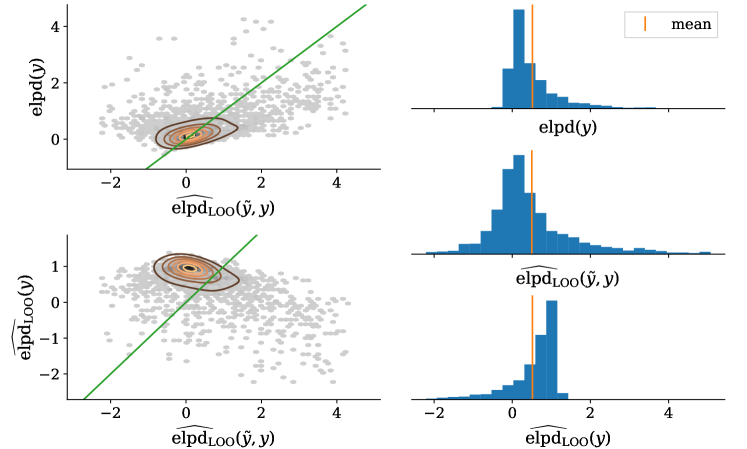
Figure 10: Comparison of ${\mathrm{elpd}\bigr{(}{\mathrm{M}_{a},\mathrm{M}_{b}}\mid y\bigl{)}}$ and the sampling distributions of ${\widehat{\mathrm{elpd}}_{\mathrm{\scriptscriptstyle LOO}}\bigr{(}{\mathrm{M}_{a},\mathrm{M}_{b}}\mid y\bigl{)}}$ and ${\widehat{\mathrm{elpd}}_{\mathrm{\scriptscriptstyle LOO}}\bigr{(}{\mathrm{M}_{a},\mathrm{M}_{b}}\mid\tilde{y},y\bigl{)}}$ for a selected problem setting, where $n=128$, $\beta_{\Delta}=0$, $r_{\star}=0$. In the joint distribution plots on the left column, kernel density estimation is shown with orange lines and the green diagonal lines corresponds to $y=x$. It can be seen from the figure, that the sampling distributions of ${\widehat{\mathrm{elpd}}_{\mathrm{\scriptscriptstyle LOO}}\bigr{(}{\mathrm{M}_{a},\mathrm{M}_{b}}\mid y\bigl{)}}$ and ${\widehat{\mathrm{elpd}}_{\mathrm{\scriptscriptstyle LOO}}\bigr{(}{\mathrm{M}_{a},\mathrm{M}_{b}}\mid\tilde{y},y\bigl{)}}$ have different shapes. For brevity, model labels are omitted in the notation in the figure.

Even though being connected, using ${\widehat{\mathrm{elpd}}_{\mathrm{\scriptscriptstyle LOO}}\bigr{(}{\mathrm{M}_{a},\mathrm{M}_{b}}\mid y,y\bigl{)}}$ as a proxy for the uncertainty in analysing the behaviour of the LOO-CV estimate would produce inaccurate results. As experimentally demonstrated in Figure 10, the connection of the data sets affects the related uncertainty of the estimator. The behaviour of ${\widehat{\mathrm{elpd}}_{\mathrm{\scriptscriptstyle LOO}}\bigr{(}{\mathrm{M}_{a},\mathrm{M}_{b}}\mid\tilde{y}^{\mathrm{obs}},y\bigl{)}}$ over possible data sets does not necessary match with the behaviour of ${\widehat{\mathrm{elpd}}_{\mathrm{\scriptscriptstyle LOO}}\bigr{(}{\mathrm{M}_{a},\mathrm{M}_{b}}\mid y\bigl{)}}$. It can be seen from the figure, that in the illustrated setting, the means of the distributions are close but the variance and skewness do not match. Additionally in the figure, the sampling distributions are compared against the distribution of ${\mathrm{elpd}\bigr{(}{\mathrm{M}_{a},\mathrm{M}_{b}}\mid y\bigl{)}}$. It can be seen that ${\widehat{\mathrm{elpd}}_{\mathrm{\scriptscriptstyle LOO}}\bigr{(}{\mathrm{M}_{a},\mathrm{M}_{b}}\mid\tilde{y},y\bigl{)}}$ has a distribution somewhat between ${\widehat{\mathrm{elpd}}_{\mathrm{\scriptscriptstyle LOO}}\bigr{(}{\mathrm{M}_{a},\mathrm{M}_{b}}\mid y\bigl{)}}$ and ${\mathrm{elpd}\bigr{(}{\mathrm{M}_{a},\mathrm{M}_{b}}\mid y\bigl{)}}$. Indeed, although not feasible in practise, it is expected that ${\widehat{\mathrm{elpd}}_{\mathrm{\scriptscriptstyle LOO}}\bigr{(}{\mathrm{M}_{a},\mathrm{M}_{b}}\mid\tilde{y},y\bigl{)}}$ would be better estimator for ${\mathrm{elpd}\bigr{(}{\mathrm{M}_{a},\mathrm{M}_{b}}\mid y\bigl{)}}$.

Appendix C Analysing the Uncertainty Estimates

The uncertainty of a LOO-CV estimate is usually estimated using normal distribution or Bayesian bootstrap. In this appendix, we discuss these estimators in more detail.

C.1 Normal Model for the Uncertainty

As discussed in Section 2.2 in Equation (9), a common approach for estimating the uncertainty in a LOO-CV estimate is to approximate it with a normal distribution as follows,

$${\widehat{\mathrm{unc}}_{\mathrm{\scriptscriptstyle LOO}}\bigr{(}{\mathrm{M}_{a},\mathrm{M}_{b}}\mid y\bigl{)}} ={\widehat{\mathrm{elpd}}_{\mathrm{\scriptscriptstyle LOO}}\bigr{(}{\mathrm{M}_{a},\mathrm{M}_{b}}\mid y\bigl{)}}-{\widehat{\mathrm{err}}_{\mathrm{\scriptscriptstyle LOO}}\bigr{(}{\mathrm{M}_{a},\mathrm{M}_{b}}\mid y\bigl{)}}\,,$$ (38)

where

$${\widehat{\mathrm{err}}_{\mathrm{\scriptscriptstyle LOO}}\bigr{(}{\mathrm{M}_{a},\mathrm{M}_{b}}\mid y\bigl{)}} \sim\operatorname{N}\mathopen{}\mathclose{{}\left(0,\,{\widehat{\mathrm{SE}}_{\mathrm{\scriptscriptstyle LOO}}\bigr{(}{\mathrm{M}_{a},\mathrm{M}_{b}}\mid y\bigl{)}}}\right)$$ (39)

is an approximation to the distribution of the true error over the possible data sets, and ${\widehat{\mathrm{SE}}_{\mathrm{\scriptscriptstyle LOO}}\bigr{(}{\mathrm{M}_{a},\mathrm{M}_{b}}\mid y\bigl{)}}$ is a naive estimator of the standard error of ${\widehat{\mathrm{elpd}}_{\mathrm{\scriptscriptstyle LOO}}\bigr{(}{\mathrm{M}_{a},\mathrm{M}_{b}}\mid y\bigl{)}}$ defined by (Vehtari et al., 2022a),

$$\mathopen{}\mathclose{{}\left({\widehat{\mathrm{SE}}_{\mathrm{\scriptscriptstyle LOO}}\bigr{(}{\mathrm{M}_{a},\mathrm{M}_{b}}\mid y\bigl{)}}}\right)^{2}$$

$$\qquad=\frac{n}{n-1}\sum_{i=1}^{n}\Bigg{(}{\widehat{\mathrm{elpd}}_{\mathrm{\scriptscriptstyle LOO},\,i}\bigr{(}{\mathrm{M}_{a},\mathrm{M}_{b}}\mid y\bigl{)}}-\frac{1}{n}\sum_{j=1}^{n}{\widehat{\mathrm{elpd}}_{\mathrm{\scriptscriptstyle LOO},\,j}\bigr{(}{\mathrm{M}_{a},\mathrm{M}_{b}}\mid y\bigl{)}}\Bigg{)}^{2}\,.$$ (40)

This estimator is motivated by the incorrect assumption that the terms ${\widehat{\mathrm{elpd}}_{\mathrm{\scriptscriptstyle LOO},\,i}\bigr{(}{\mathrm{M}_{a},\mathrm{M}_{b}}\mid y\bigl{)}}$ are independent. In reality, since each observation is a part of $n-1$ training sets, the variance $\operatorname{Var}\mathopen{}\mathclose{{}\left({\widehat{\mathrm{elpd}}_{\mathrm{\scriptscriptstyle LOO}}\bigr{(}{\mathrm{M}_{a},\mathrm{M}_{b}}\mid y\bigl{)}}}\right)$ depends on both the variance of each ${\widehat{\mathrm{elpd}}_{\mathrm{\scriptscriptstyle LOO},\,i}\bigr{(}{\mathrm{M}_{a},\mathrm{M}_{b}}\mid y\bigl{)}}$ and on the dependency between the different folds. In the following propositions 8 and 9 and in the Corollary 10, we present the associated bias with the naive variance estimator in the context of model comparison.

Proposition 8

Let ${L}_{{k},i}={\widehat{\mathrm{elpd}}_{\mathrm{\scriptscriptstyle LOO},\,i}\bigr{(}{\mathrm{M}_{k}}\mid y\bigl{)}}$ and ${L}_{{a-b},i}={\widehat{\mathrm{elpd}}_{\mathrm{\scriptscriptstyle LOO},\,i}\bigr{(}{\mathrm{M}_{a},\mathrm{M}_{b}}\mid y\bigl{)}}$ and

$$\operatorname{Var}\mathopen{}\mathclose{{}\left({L}_{{a-b},i}}\right) =\sigma^{2}_{a-b} \operatorname{Cov}\mathopen{}\mathclose{{}\left({L}_{{a-b},i},{L}_{{a-b},j}}\right) =\gamma_{{a-b}}$$

$$\operatorname{Var}\mathopen{}\mathclose{{}\left({L}_{{k},i}}\right) =\sigma^{2}_{k} \operatorname{Cov}\mathopen{}\mathclose{{}\left({L}_{{k},i},{L}_{{k},j}}\right) =\gamma_{{k}}$$

$$\operatorname{Cov}\mathopen{}\mathclose{{}\left({L}_{{a},i},{L}_{{b},i}}\right) =\rho_{{a}{b}} \operatorname{Cov}\mathopen{}\mathclose{{}\left({L}_{{a},i},{L}_{{b},j}}\right) =\gamma_{{a}{b}}\,,$$ (41)

where $i\neq j$ and ${\mathrm{M}_{k}}\in\{{\mathrm{M}_{a}},{\mathrm{M}_{b}}\}$. Now

$$\operatorname{Var}\mathopen{}\mathclose{{}\left({\widehat{\mathrm{elpd}}_{\mathrm{\scriptscriptstyle LOO}}\bigr{(}{\mathrm{M}_{a},\mathrm{M}_{b}}\mid y\bigl{)}}}\right) =n\sigma^{2}_{a-b}+n(n-1)\gamma_{a-b}$$

$$=n\mathopen{}\mathclose{{}\left(\sigma^{2}_{a}+\sigma^{2}_{b}-2\rho_{{a}{b}}}\right)+n(n-1)\mathopen{}\mathclose{{}\left(\gamma_{a}+\gamma_{b}-2\gamma_{{a}{b}}}\right)\,.$$ (42)

Proof  We have

$$\operatorname{Var}\mathopen{}\mathclose{{}\left({\widehat{\mathrm{elpd}}_{\mathrm{\scriptscriptstyle LOO}}\bigr{(}{\mathrm{M}_{a},\mathrm{M}_{b}}\mid y\bigl{)}}}\right)$$

$$\qquad=\sum_{i=1}^{n}\sum_{j=1}^{n}\operatorname{Cov}\mathopen{}\mathclose{{}\left({L}_{{a},i}-{L}_{{b},i},{L}_{{a},j}-{L}_{{b},j}}\right)$$

$$\qquad=\sum_{i=1}^{n}\sum_{j=1}^{n}\Big{(}\operatorname{Cov}({L}_{{a},i},{L}_{{a},j})+\operatorname{Cov}({L}_{{b},i},{L}_{{b},j})$$

$$\qquad\qquad\qquad-\operatorname{Cov}({L}_{{a},i},{L}_{{b},j})-\operatorname{Cov}({L}_{{b},i},{L}_{{a},j})\Big{)}$$

$$\qquad=\sum_{i=1}^{n}\Big{(}\operatorname{Var}({L}_{{a},i})+{L}_{{b},i}-2\operatorname{Cov}({L}_{{a},i},{L}_{{b},i})\Big{)}$$

$$\qquad\qquad\qquad+\sum_{i=1}^{n}\sum_{j\neq i}\Big{(}\operatorname{Cov}({L}_{{a},i},{L}_{{a},j})+\operatorname{Cov}({L}_{{b},i},{L}_{{b},j})-2\operatorname{Cov}({L}_{{a},i},{L}_{{b},j})\Big{)}$$

$$\qquad=n\mathopen{}\mathclose{{}\left(\sigma^{2}_{a}+\sigma^{2}_{b}-2\rho_{{a}{b}}}\right)+n(n-1)\mathopen{}\mathclose{{}\left(\gamma_{a}+\gamma_{b}-2\gamma_{{a}{b}}}\right)\,.$$ (43)

 

Proposition 9

Following the definitions in Proposition 8, the expectation of the variance estimator $\widehat{\mathrm{SE}}_{\mathrm{\scriptscriptstyle LOO}}$ in Equation (40) is

$$\operatorname{E}\mathopen{}\mathclose{{}\left[{\widehat{\mathrm{SE}}_{\mathrm{\scriptscriptstyle LOO}}\bigr{(}{\mathrm{M}_{a},\mathrm{M}_{b}}\mid y\bigl{)}}^{2}}\right] =n\sigma^{2}_{a-b}-n\gamma_{a-b}$$

$$=n\mathopen{}\mathclose{{}\left(\sigma^{2}_{a}+\sigma^{2}_{b}-2\rho_{{a}{b}}}\right)-n\mathopen{}\mathclose{{}\left(\gamma_{a}+\gamma_{b}-2\gamma_{{a}{b}}}\right).$$ (44)

Proof  We have

$$\operatorname{E}\mathopen{}\mathclose{{}\left[{L}_{{a-b},i}^{2}}\right] =\operatorname{E}\mathopen{}\mathclose{{}\left[{L}_{{a-b},i}}\right]^{2}+\operatorname{Var}\mathopen{}\mathclose{{}\left({L}_{{a-b},i}}\right)$$ (45)

$$\operatorname{E}\mathopen{}\mathclose{{}\left[{L}_{{a-b},i}{L}_{{a-b},j}}\right] =\operatorname{E}\mathopen{}\mathclose{{}\left[{L}_{{a-b},i}}\right]\operatorname{E}\mathopen{}\mathclose{{}\left[{L}_{{a-b},j}}\right]+\operatorname{Cov}\mathopen{}\mathclose{{}\left({L}_{{a-b},i},{L}_{{a-b},j}}\right),\quad i\neq j.$$ (46)

Now

$$\operatorname{E}\mathopen{}\mathclose{{}\left[\mathopen{}\mathclose{{}\left({\widehat{\mathrm{SE}}_{\mathrm{\scriptscriptstyle LOO}}\bigr{(}{\mathrm{M}_{a},\mathrm{M}_{b}}\mid y\bigl{)}}}\right)^{2}}\right]$$

$$\qquad=\operatorname{E}\mathopen{}\mathclose{{}\left[\frac{n}{n-1}\sum_{i=1}^{n}\mathopen{}\mathclose{{}\left({L}_{{a-b},i}-\frac{1}{n}\sum_{j=1}^{n}{L}_{{a-b},j}}\right)^{2}}\right]$$

$$\qquad=\frac{n}{n-1}\sum_{i=1}^{n}\operatorname{E}\mathopen{}\mathclose{{}\left[{L}_{{a-b},i}^{2}-\frac{2}{n}{L}_{{a-b},i}\sum_{j=1}^{n}{L}_{{a-b},j}+\mathopen{}\mathclose{{}\left(\frac{1}{n}\sum_{j=1}^{n}{L}_{{a-b},j}}\right)^{2}}\right]$$

$$\qquad=\frac{n}{n-1}\sum_{i=1}^{n}\mathopen{}\mathclose{{}\left[\operatorname{E}\mathopen{}\mathclose{{}\left[{L}_{{a-b},i}^{2}}\right]-\frac{2}{n}\mathopen{}\mathclose{{}\left(\operatorname{E}\mathopen{}\mathclose{{}\left[{L}_{{a-b},i}^{2}}\right]+\sum_{j\neq i}\operatorname{E}\mathopen{}\mathclose{{}\left[{L}_{{a-b},i}{L}_{{a-b},j}}\right]}\right)}\right.$$

$$\qquad\mathopen{}\mathclose{{}\left.\hskip 71.13188pt+\frac{1}{n^{2}}\mathopen{}\mathclose{{}\left(\sum_{j=1}^{n}\operatorname{E}\mathopen{}\mathclose{{}\left[{L}_{{a-b},j}^{2}}\right]+\sum_{j=1}^{n}\sum_{p\neq j}\operatorname{E}\mathopen{}\mathclose{{}\left[{L}_{{a-b},j}{L}_{{a-b},p}}\right]}\right)}\right]$$

$$\qquad=\frac{n}{n-1}\sum_{i=1}^{n}\Bigg{[}\operatorname{E}\mathopen{}\mathclose{{}\left[{L}_{{a-b},i}}\right]^{2}+\operatorname{Var}\mathopen{}\mathclose{{}\left({L}_{{a-b},i}}\right)$$

$$\qquad\hskip 71.13188pt-\frac{2}{n}\Big{(}\operatorname{E}\mathopen{}\mathclose{{}\left[{L}_{{a-b},i}}\right]^{2}+\operatorname{Var}\mathopen{}\mathclose{{}\left({L}_{{a-b},i}}\right)+(n-1)(\operatorname{E}\mathopen{}\mathclose{{}\left[{L}_{{a-b},i}}\right]^{2}$$

$$\qquad\hskip 113.81102pt+\operatorname{Cov}\mathopen{}\mathclose{{}\left({L}_{{a-b},i},{L}_{{a-b},j}}\right))\Big{)}$$

$$\qquad\hskip 71.13188pt+\frac{1}{n^{2}}\Big{(}n(\operatorname{E}\mathopen{}\mathclose{{}\left[{L}_{{a-b},i}}\right]^{2}+\operatorname{Var}\mathopen{}\mathclose{{}\left({L}_{{a-b},i}}\right))+n(n-1)(\operatorname{E}\mathopen{}\mathclose{{}\left[{L}_{{a-b},i}}\right]^{2}$$

$$\qquad\hskip 113.81102pt+\operatorname{Cov}\mathopen{}\mathclose{{}\left({L}_{{a-b},i},{L}_{{a-b},j}}\right))\Big{)}\Bigg{]}$$

$$\qquad=\frac{n}{n-1}\sum_{i=1}^{n}\mathopen{}\mathclose{{}\left[\mathopen{}\mathclose{{}\left(1-\frac{2n}{n}+\frac{n^{2}}{n^{2}}}\right)\operatorname{E}\mathopen{}\mathclose{{}\left[{L}_{{a-b},i}}\right]^{2}+\mathopen{}\mathclose{{}\left(1-\frac{2}{n}+\frac{n}{n^{2}}}\right)\operatorname{Var}\mathopen{}\mathclose{{}\left({L}_{{a-b},i}}\right)}\right.$$

$$\qquad\mathopen{}\mathclose{{}\left.\hskip 71.13188pt+\mathopen{}\mathclose{{}\left(-\frac{2(n-1)}{n}+\frac{n(n-1)}{n^{2}}}\right)\operatorname{Cov}\mathopen{}\mathclose{{}\left({L}_{{a-b},i},{L}_{{a-b},j}}\right)}\right]$$

$$\qquad=\frac{n}{n-1}\sum_{i=1}^{n}\mathopen{}\mathclose{{}\left[\frac{n-1}{n}\operatorname{Var}\mathopen{}\mathclose{{}\left({L}_{{a-b},i}}\right)-\frac{n-1}{n}\operatorname{Cov}\mathopen{}\mathclose{{}\left({L}_{{a-b},i},{L}_{{a-b},j}}\right)}\right]$$

$$\qquad=n\operatorname{Var}\mathopen{}\mathclose{{}\left({L}_{{a-b},i}}\right)-n\operatorname{Cov}\mathopen{}\mathclose{{}\left({L}_{{a-b},i},{L}_{{a-b},j}}\right)$$

$$\qquad=n\sigma^{2}_{a-b}-n\gamma_{a-b}\,,$$ (47)

and furthermore

$$\operatorname{E}\mathopen{}\mathclose{{}\left[\mathopen{}\mathclose{{}\left({\widehat{\mathrm{SE}}_{\mathrm{\scriptscriptstyle LOO}}\bigr{(}{\mathrm{M}_{a},\mathrm{M}_{b}}\mid y\bigl{)}}}\right)^{2}}\right] =n\operatorname{Var}\mathopen{}\mathclose{{}\left({L}_{{a},i}-{L}_{{b},i}}\right)$$

$$\quad-n\operatorname{Cov}\mathopen{}\mathclose{{}\left({L}_{{a},i}-{L}_{{b},i},{L}_{{a},j}-{L}_{{b},j}}\right)$$

$$=n\mathopen{}\mathclose{{}\left(\operatorname{Var}({L}_{{a},i})+\operatorname{Var}({L}_{{b},i})-2\operatorname{Cov}({L}_{{a},i},{L}_{{b},i})}\right)$$

$$\quad-n\mathopen{}\mathclose{{}\left(\operatorname{Cov}\mathopen{}\mathclose{{}\left({L}_{{a},i},{L}_{{a},j}}\right)+\operatorname{Cov}\mathopen{}\mathclose{{}\left({L}_{{b},i},{L}_{{b},j}}\right)-2\operatorname{Cov}\mathopen{}\mathclose{{}\left({L}_{{a},i},{L}_{{b},j}}\right)}\right)$$

$$=n\mathopen{}\mathclose{{}\left(\sigma^{2}_{a}+\sigma^{2}_{b}-2\rho_{{a}{b}}}\right)$$

$$\quad-n\mathopen{}\mathclose{{}\left(\gamma_{a}+\gamma_{b}-2\gamma_{{a}{b}}}\right)\,.$$ (48)

 

Corollary 10

Following the definitions in Proposition 8, the estimator ${\widehat{\mathrm{SE}}_{\mathrm{\scriptscriptstyle LOO}}\bigr{(}{\mathrm{M}_{a},\mathrm{M}_{b}}\mid y\bigl{)}}^{2}$ defined in Equation (40) for the variance $\operatorname{Var}\mathopen{}\mathclose{{}\left({\widehat{\mathrm{elpd}}_{\mathrm{\scriptscriptstyle LOO}}\bigr{(}{\mathrm{M}_{a},\mathrm{M}_{b}}\mid y\bigl{)}}}\right)$ has a bias of

$$\operatorname{E}\mathopen{}\mathclose{{}\left[{\widehat{\mathrm{SE}}_{\mathrm{\scriptscriptstyle LOO}}\bigr{(}{\mathrm{M}_{a},\mathrm{M}_{b}}\mid y\bigl{)}}^{2}}\right]-\operatorname{Var}\mathopen{}\mathclose{{}\left({\widehat{\mathrm{elpd}}_{\mathrm{\scriptscriptstyle LOO}}\bigr{(}{\mathrm{M}_{a},\mathrm{M}_{b}}\mid y\bigl{)}}}\right)=-n^{2}\gamma_{a-b}=-n^{2}\mathopen{}\mathclose{{}\left(\gamma_{a}+\gamma_{b}-2\gamma_{{a}{b}}}\right)\,.$$ (49)

Proof  The ${\mathrm{elpd}\bigr{(}{a-b}\mid y\bigl{)}}$, i.e. the true variance $\operatorname{Var}\mathopen{}\mathclose{{}\left({\widehat{\mathrm{elpd}}_{\mathrm{\scriptscriptstyle LOO}}\bigr{(}{\mathrm{M}_{a},\mathrm{M}_{b}}\mid y\bigl{)}}}\right)$, is given in Proposition 8. The expectation of the estimator ${\widehat{\mathrm{SE}}_{\mathrm{\scriptscriptstyle LOO}}\bigr{(}{\mathrm{M}_{a},\mathrm{M}_{b}}\mid y\bigl{)}}^{2}$ is given in Proposition 9. The resulting bias follows directly from these propositions.  

C.2 Dirichlet Model for the Uncertainty

As discussed in Section 2.2, an alternative way to address the uncertainty is to use a Bayesian bootstrap procedure (Rubin, 1981; Vehtari and Lampinen, 2002)to model $p({\mathrm{unc}_{\mathrm{\scriptscriptstyle LOO}}\bigr{(}{\mathrm{M}_{a},\mathrm{M}_{b}}\mid y\bigl{)}})$. Compared to the normal approximation, while being able to represent skewness, also this method has problems with higher moments and heavy tailed distributions (Rubin, 1981).

C.3 Not Considering All the Terms in the Error

As discussed in Section 2.3, in addition to possibly inaccurately approximating the variability in ${\widehat{\mathrm{elpd}}_{\mathrm{\scriptscriptstyle LOO}}\bigr{(}{\mathrm{M}_{a},\mathrm{M}_{b}}\mid y\bigl{)}}$, the presented ways of estimating the uncertainty can be poor representations of the uncertainty about ${\mathrm{unc}_{\mathrm{\scriptscriptstyle LOO}}\bigr{(}{\mathrm{M}_{a},\mathrm{M}_{b}}\mid y\bigl{)}}$ because they are based on estimating the sampling distribution, which can have only a weak connection to the error distribution. As seen from the formulation of the error ${\mathrm{err}_{\mathrm{\scriptscriptstyle LOO}}\bigr{(}{\mathrm{M}_{a},\mathrm{M}_{b}}\mid y\bigl{)}}$ presented in Equation (38), an estimator based on the sampling distribution does not consider the effect of the term ${\mathrm{elpd}\bigr{(}{\mathrm{M}_{a},\mathrm{M}_{b}}\mid y\bigl{)}}$. As demonstrated in figures 17 and 18 in Appendix E, while in well behaved problem settings the variability of the sampling distribution ${\widehat{\mathrm{elpd}}_{\mathrm{\scriptscriptstyle LOO}}\bigr{(}{\mathrm{M}_{a},\mathrm{M}_{b}}\mid y\bigl{)}}$ can match with the variability of the error ${\mathrm{err}_{\mathrm{\scriptscriptstyle LOO}}\bigr{(}{\mathrm{M}_{a},\mathrm{M}_{b}}\mid y\bigl{)}}$, in problematic situations they do not match. As a comparison, when estimating e-elpd instead of ${\mathrm{elpd}}{}$, the variance of the sampling distribution corresponds to the variance of the error distribution, as discussed in Appendix A, and estimating the sampling distribution is sufficient in estimating the uncertainty of the LOO-CV estimate.

Appendix D Normal Linear Regression Case Study

In this appendix, we derive the analytic form for the approximation error ${\mathrm{err}_{\mathrm{\scriptscriptstyle LOO}}\bigr{(}{\mathrm{M}_{a},\mathrm{M}_{b}}\mid y\bigl{)}}={\widehat{\mathrm{elpd}}_{\mathrm{\scriptscriptstyle LOO}}\bigr{(}{\mathrm{M}_{a},\mathrm{M}_{b}}\mid y\bigl{)}}-{\mathrm{elpd}\bigr{(}{\mathrm{M}_{a}},{\mathrm{M}_{b}}\mid y\bigl{)}}$ in a normal linear regression model comparison setting under known data generating mechanism. In addition, we derive the analytic forms for ${\mathrm{elpd}\bigr{(}\cdots\mid y\bigl{)}}$ and ${\widehat{\mathrm{elpd}}_{\mathrm{\scriptscriptstyle LOO}}\bigr{(}\cdots\mid y\bigl{)}}$ for the individual models and for the difference.

Consider the following data generation mechanism defined in Section 3, we compare two nested normal linear regression models $\mathrm{M_{A}}$ and $\mathrm{M_{B}}$, both considering a subset of covariates. Let $X_{[\boldsymbol{\cdot},{k}]}$ and $\beta_{{k}}$ denote the explanatory variable matrix and respective effect vector including only the covariates considered by model ${\mathrm{M}_{k}}\in\{{\mathrm{M_{A}}},{\mathrm{M_{B}}}\}$. Correspondingly, let $X_{[\boldsymbol{\cdot},-{k}]}$ and $\beta_{-{k}}$ denote the explanatory variable matrix and respective effect vector including only the covariates not considered by model ${\mathrm{M}_{k}}$. If a model includes all the covariates, we define that $X_{[\boldsymbol{\cdot},-{k}]}$ is a column vector of length $n$ of zeroes and $\beta_{-{k}}=0$. We assume that there exists at least one covariate that is included in one model but not in the other, so that there is some difference in the models. Otherwise ${\mathrm{elpd}\bigr{(}{\mathrm{M_{A},M_{B}}}\mid y\bigl{)}}$ and ${\widehat{\mathrm{elpd}}_{\mathrm{\scriptscriptstyle LOO}}\bigr{(}{\mathrm{M_{A},M_{B}}}\mid y\bigl{)}}$ would be trivially always zero. In both models, the noise variance $\tau^{2}$ is fixed and $\widehat{\beta}_{k}$ is the respective sole estimated unknown model parameter. We apply uniform prior distribution for both models. Hence we have the following forms for the likelihood, posterior distribution, and posterior predictive distribution for model ${\mathrm{M}_{k}}$: (see e.g. Gelman et al., 2013, pp. 355–357)

$$y|\widehat{\beta}_{k},X_{[\boldsymbol{\cdot},{k}]},\tau \sim\operatorname{N}\mathopen{}\mathclose{{}\left(X_{[\boldsymbol{\cdot},{k}]}\widehat{\beta}_{k},\;\tau^{2}\mathrm{I}}\right),$$ (50)

$$\widehat{\beta}_{k}|y,X_{[\boldsymbol{\cdot},{k}]},\tau \sim\operatorname{N}\mathopen{}\mathclose{{}\left((X_{[\boldsymbol{\cdot},{k}]}^{\mathchoice{\raisebox{2.6pt}{$\scriptstyle\mathrm{T}$}}{\raisebox{2.6pt}{$\scriptstyle\mathrm{T}$}}{\raisebox{1.0pt}{$\scriptscriptstyle\mathrm{T}$}}{\raisebox{0.5pt}{\tiny$\scriptscriptstyle\mathrm{T}$}}}X_{[\boldsymbol{\cdot},{k}]})^{-1}X_{[\boldsymbol{\cdot},{k}]}^{\mathchoice{\raisebox{2.6pt}{$\scriptstyle\mathrm{T}$}}{\raisebox{2.6pt}{$\scriptstyle\mathrm{T}$}}{\raisebox{1.0pt}{$\scriptscriptstyle\mathrm{T}$}}{\raisebox{0.5pt}{\tiny$\scriptscriptstyle\mathrm{T}$}}}y,\;(X_{[\boldsymbol{\cdot},{k}]}^{\mathchoice{\raisebox{2.6pt}{$\scriptstyle\mathrm{T}$}}{\raisebox{2.6pt}{$\scriptstyle\mathrm{T}$}}{\raisebox{1.0pt}{$\scriptscriptstyle\mathrm{T}$}}{\raisebox{0.5pt}{\tiny$\scriptscriptstyle\mathrm{T}$}}}X_{[\boldsymbol{\cdot},{k}]})^{-1}\tau^{2}}\right),$$ (51)

$$\widetilde{y}|y,X_{[\boldsymbol{\cdot},{k}]},\widetilde{x},\tau \sim\operatorname{N}\mathopen{}\mathclose{{}\left(\widetilde{x}(X_{[\boldsymbol{\cdot},{k}]}^{\mathchoice{\raisebox{2.6pt}{$\scriptstyle\mathrm{T}$}}{\raisebox{2.6pt}{$\scriptstyle\mathrm{T}$}}{\raisebox{1.0pt}{$\scriptscriptstyle\mathrm{T}$}}{\raisebox{0.5pt}{\tiny$\scriptscriptstyle\mathrm{T}$}}}X_{[\boldsymbol{\cdot},{k}]})^{-1}X_{[\boldsymbol{\cdot},{k}]}^{\mathchoice{\raisebox{2.6pt}{$\scriptstyle\mathrm{T}$}}{\raisebox{2.6pt}{$\scriptstyle\mathrm{T}$}}{\raisebox{1.0pt}{$\scriptscriptstyle\mathrm{T}$}}{\raisebox{0.5pt}{\tiny$\scriptscriptstyle\mathrm{T}$}}}y,\;\mathopen{}\mathclose{{}\left(1+\widetilde{x}(X_{[\boldsymbol{\cdot},{k}]}^{\mathchoice{\raisebox{2.6pt}{$\scriptstyle\mathrm{T}$}}{\raisebox{2.6pt}{$\scriptstyle\mathrm{T}$}}{\raisebox{1.0pt}{$\scriptscriptstyle\mathrm{T}$}}{\raisebox{0.5pt}{\tiny$\scriptscriptstyle\mathrm{T}$}}}X_{[\boldsymbol{\cdot},{k}]})^{-1}\widetilde{x}^{\mathchoice{\raisebox{2.6pt}{$\scriptstyle\mathrm{T}$}}{\raisebox{2.6pt}{$\scriptstyle\mathrm{T}$}}{\raisebox{1.0pt}{$\scriptscriptstyle\mathrm{T}$}}{\raisebox{0.5pt}{\tiny$\scriptscriptstyle\mathrm{T}$}}}}\right)\tau^{2}}\right),$$ (52)

where $\widetilde{y},\widetilde{x}$ is a test observation with a scalar response variable and conformable explanatory variable row vector respectively.

D.1 Elpd

In this section we find the analytic form for ${\mathrm{elpd}\bigr{(}{\mathrm{M}_{k}}\mid y\bigl{)}}$ for model ${\mathrm{M}_{k}}\in\{{\mathrm{M_{A}}},{\mathrm{M_{B}}}\}$. We have

$${\mathrm{elpd}\bigr{(}{\mathrm{M}_{k}}\mid y\bigl{)}} =\sum_{i=1}^{n}\int_{-\infty}^{\infty}p_{\text{true}}(\tilde{y}_{i})\log p_{k}(\tilde{y}_{i}|y)\mathop{}\kern-2.0pt\mathrm{d}\tilde{y}_{i}\,,$$ (53)

$$p_{\text{true}}(\tilde{y}_{i}) =\operatorname{N}\mathopen{}\mathclose{{}\left(\tilde{y}_{i}\middle|\widetilde{\mu}_{i},\widetilde{\sigma}_{i}}\right),$$ (54)

$$p_{k}(\tilde{y}_{i}|y) =\operatorname{N}\mathopen{}\mathclose{{}\left(\tilde{y}_{i}\middle|\mu_{{k},\,i},\sigma_{{k},\,i}}\right),$$ (55)

where

$$\widetilde{\mu}_{i} =\mu_{\star,\,i}+X_{[i,\boldsymbol{\cdot}]}\beta$$ (56)

$$\widetilde{\sigma}_{i}^{2} =\sigma_{\star,\,i}^{2}$$ (57)

and, according to Equation (52),

$$\mu_{{k},\,i} =X_{[i,{k}]}\mathopen{}\mathclose{{}\left(X_{[\boldsymbol{\cdot},{k}]}^{\mathchoice{\raisebox{2.6pt}{$\scriptstyle\mathrm{T}$}}{\raisebox{2.6pt}{$\scriptstyle\mathrm{T}$}}{\raisebox{1.0pt}{$\scriptscriptstyle\mathrm{T}$}}{\raisebox{0.5pt}{\tiny$\scriptscriptstyle\mathrm{T}$}}}X_{[\boldsymbol{\cdot},{k}]}}\right)^{-1}X_{[\boldsymbol{\cdot},{k}]}^{\mathchoice{\raisebox{2.6pt}{$\scriptstyle\mathrm{T}$}}{\raisebox{2.6pt}{$\scriptstyle\mathrm{T}$}}{\raisebox{1.0pt}{$\scriptscriptstyle\mathrm{T}$}}{\raisebox{0.5pt}{\tiny$\scriptscriptstyle\mathrm{T}$}}}y$$ (58)

$$\sigma_{{k},\,i}^{2} =\mathopen{}\mathclose{{}\left(1+X_{[i,{k}]}\mathopen{}\mathclose{{}\left(X_{[\boldsymbol{\cdot},{k}]}^{\mathchoice{\raisebox{2.6pt}{$\scriptstyle\mathrm{T}$}}{\raisebox{2.6pt}{$\scriptstyle\mathrm{T}$}}{\raisebox{1.0pt}{$\scriptscriptstyle\mathrm{T}$}}{\raisebox{0.5pt}{\tiny$\scriptscriptstyle\mathrm{T}$}}}X_{[\boldsymbol{\cdot},{k}]}}\right)^{-1}X_{[i,{k}]}^{\mathchoice{\raisebox{2.6pt}{$\scriptstyle\mathrm{T}$}}{\raisebox{2.6pt}{$\scriptstyle\mathrm{T}$}}{\raisebox{1.0pt}{$\scriptscriptstyle\mathrm{T}$}}{\raisebox{0.5pt}{\tiny$\scriptscriptstyle\mathrm{T}$}}}}\right)\tau^{2}$$ (59)

for $i=1,2,\dots,n$. The distributions can be formulated as

$$p_{\text{true}}(\tilde{y}_{i}) =(2\pi\widetilde{\sigma}_{i}^{2})^{-1/2}\exp\mathopen{}\mathclose{{}\left(-\frac{1}{2}\mathopen{}\mathclose{{}\left(\frac{\tilde{y}_{i}-\widetilde{\mu}_{i}}{\widetilde{\sigma}_{i}}}\right)^{2}}\right)$$

$$=c\,\exp\mathopen{}\mathclose{{}\left(-a\tilde{y}_{i}^{2}+b\tilde{y}_{i}}\right)\,,$$ (60)

where

$$a =\frac{1}{2\widetilde{\sigma}_{i}^{2}}>0\,, b =\frac{\widetilde{\mu}_{i}}{\widetilde{\sigma}_{i}^{2}}\,, c =\exp\mathopen{}\mathclose{{}\left(-\frac{\widetilde{\mu}_{i}^{2}}{2\widetilde{\sigma}_{i}^{2}}-\frac{1}{2}\log\mathopen{}\mathclose{{}\left(2\pi\widetilde{\sigma}_{i}^{2}}\right)}\right)\,,$$ (61)

and

$$\log p_{k}(\tilde{y}_{i}|y) =-\frac{1}{2}\mathopen{}\mathclose{{}\left(\frac{\tilde{y}_{i}-\mu_{{k},\,i}}{\sigma_{{k},\,i}}}\right)^{2}-\frac{1}{2}\log\mathopen{}\mathclose{{}\left(2\pi\sigma_{{k},\,i}^{2}}\right)$$

$$=-p\tilde{y}_{i}^{2}+q\tilde{y}_{i}+r\,,$$ (62)

where

$$p =\frac{1}{2\sigma_{{k},\,i}^{2}}>0\,, q =\frac{\mu_{{k},\,i}}{\sigma_{{k},\,i}^{2}}\,, r =-\frac{\mu_{{k},\,i}^{2}}{2\sigma_{{k},\,i}^{2}}-\frac{1}{2}\log\mathopen{}\mathclose{{}\left(2\pi\sigma_{{k},\,i}^{2}}\right)\,.$$ (63)

Now

$$\int_{-\infty}^{\infty}p_{\text{true}}(\tilde{y}_{i})\log p_{k}(\tilde{y}_{i}|y)\mathop{}\kern-2.0pt\mathrm{d}\tilde{y}_{i}$$

$$\qquad=-cp\int_{-\infty}^{\infty}\tilde{y}_{i}^{2}\exp\mathopen{}\mathclose{{}\left(-a\tilde{y}_{i}^{2}+b\tilde{y}_{i}}\right)\mathop{}\kern-2.0pt\mathrm{d}\tilde{y}_{i}$$

$$\qquad\quad+cq\int_{-\infty}^{\infty}\tilde{y}_{i}\exp\mathopen{}\mathclose{{}\left(-a\tilde{y}_{i}^{2}+b\tilde{y}_{i}}\right)\mathop{}\kern-2.0pt\mathrm{d}\tilde{y}_{i}$$

$$\qquad\quad+cr\int_{-\infty}^{\infty}\exp\mathopen{}\mathclose{{}\left(-a\tilde{y}_{i}^{2}+b\tilde{y}_{i}}\right)\mathop{}\kern-2.0pt\mathrm{d}\tilde{y}_{i}\,.$$ (64)

These integrals are

$$\int_{-\infty}^{\infty}\tilde{y}_{i}^{2}\exp\mathopen{}\mathclose{{}\left(-a\tilde{y}_{i}^{2}+b\tilde{y}_{i}}\right)\mathop{}\kern-2.0pt\mathrm{d}\tilde{y}_{i} =\frac{\sqrt{\pi}}{2a^{3/2}}\mathopen{}\mathclose{{}\left(\frac{b^{2}}{2a}+1}\right)\exp\mathopen{}\mathclose{{}\left(\frac{b^{2}}{4a}}\right)$$ (65)

(Jeffrey and Zwillinger, 2000, p. 360, Section 3.462, Eq 22.8),

$$\int_{-\infty}^{\infty}\tilde{y}_{i}\exp\mathopen{}\mathclose{{}\left(-a\tilde{y}_{i}^{2}+b\tilde{y}_{i}}\right)\mathop{}\kern-2.0pt\mathrm{d}\tilde{y}_{i} =\frac{\sqrt{\pi}b}{2a^{3/2}}\exp\mathopen{}\mathclose{{}\left(\frac{b^{2}}{4a}}\right)$$ (66)

(Jeffrey and Zwillinger, 2000, p. 360, Section 3.462, Eq 22.8), and

$$\int_{-\infty}^{\infty}\exp\mathopen{}\mathclose{{}\left(-a\tilde{y}_{i}^{2}+b\tilde{y}_{i}}\right)\mathop{}\kern-2.0pt\mathrm{d}\tilde{y}_{i} =\frac{\sqrt{\pi}}{a^{1/2}}\exp\mathopen{}\mathclose{{}\left(\frac{b^{2}}{4a}}\right)$$ (67)

(Jeffrey and Zwillinger, 2000, p. 333, Section 3.323, Eq 2.10). Now we can simplify

$$\int_{-\infty}^{\infty}p_{\text{true}}(\tilde{y}_{i})\log p_{k}(\tilde{y}_{i}|y)\mathop{}\kern-2.0pt\mathrm{d}\tilde{y}_{i}$$

$$\qquad=\sqrt{\pi}\exp\mathopen{}\mathclose{{}\left(\frac{b^{2}}{4a}+\log c}\right)\mathopen{}\mathclose{{}\left(-\frac{pb^{2}}{4a^{5/2}}-\frac{p}{2a^{3/2}}+\frac{qb}{2a^{3/2}}+\frac{r}{a^{1/2}}}\right)$$

$$\qquad=\sqrt{\pi}\mathopen{}\mathclose{{}\left(2\pi\widetilde{\sigma}_{i}^{2}}\right)^{-1/2}\mathopen{}\mathclose{{}\left(-\sqrt{2}p\widetilde{\mu}_{i}^{2}\widetilde{\sigma}_{i}-\sqrt{2}p\widetilde{\sigma}_{i}^{3}+\sqrt{2}q\widetilde{\mu}_{i}\widetilde{\sigma}_{i}+\sqrt{2}r\widetilde{\sigma}_{i}}\right)$$

$$\qquad=-p\widetilde{\mu}_{i}^{2}-p\widetilde{\sigma}_{i}^{2}+q\widetilde{\mu}_{i}+r$$

$$\qquad=\frac{-\widetilde{\mu}_{i}^{2}-\widetilde{\sigma}_{i}^{2}+2\widetilde{\mu}_{i}\mu_{{k},\,i}-\mu_{{k},\,i}^{2}}{2\sigma_{{k},\,i}^{2}}-\frac{1}{2}\log\mathopen{}\mathclose{{}\left(2\pi\sigma_{{k},\,i}^{2}}\right)$$

$$\qquad=-\frac{\mathopen{}\mathclose{{}\left(\mu_{{k},\,i}-\widetilde{\mu}_{i}}\right)^{2}+\widetilde{\sigma}_{i}^{2}}{2\sigma_{{k},\,i}^{2}}-\frac{1}{2}\log\mathopen{}\mathclose{{}\left(2\pi\sigma_{{k},\,i}^{2}}\right)\,.$$ (68)

Let $P_{{k}}$ be the following orthogonal projection matrix for model $\mathrm{M}_{k}$:

$$P_{{k}} =X_{[\boldsymbol{\cdot},{k}]}\mathopen{}\mathclose{{}\left(X_{[\boldsymbol{\cdot},{k}]}^{\mathchoice{\raisebox{2.6pt}{$\scriptstyle\mathrm{T}$}}{\raisebox{2.6pt}{$\scriptstyle\mathrm{T}$}}{\raisebox{1.0pt}{$\scriptscriptstyle\mathrm{T}$}}{\raisebox{0.5pt}{\tiny$\scriptscriptstyle\mathrm{T}$}}}X_{[\boldsymbol{\cdot},{k}]}}\right)^{-1}X_{[\boldsymbol{\cdot},{k}]}^{\mathchoice{\raisebox{2.6pt}{$\scriptstyle\mathrm{T}$}}{\raisebox{2.6pt}{$\scriptstyle\mathrm{T}$}}{\raisebox{1.0pt}{$\scriptscriptstyle\mathrm{T}$}}{\raisebox{0.5pt}{\tiny$\scriptscriptstyle\mathrm{T}$}}}$$ (69)

so that

$$\mu_{{k},\,i} =P_{{k}[i,\boldsymbol{\cdot}]}y$$

$$=P_{{k}[i,\boldsymbol{\cdot}]}\mathopen{}\mathclose{{}\left(X\beta+\varepsilon}\right)$$

$$=P_{{k}[i,\boldsymbol{\cdot}]}X\beta+P_{{k}[i,\boldsymbol{\cdot}]}\varepsilon$$ (70)

$$\sigma_{{k},\,i}^{2} =\big{(}1+P_{{k}[i,i]}\big{)}\tau^{2}\,.$$ (71)

Now we can write

$$\mathopen{}\mathclose{{}\left(\mu_{{k},\,i}-\widetilde{\mu}_{i}}\right)^{2} =\mathopen{}\mathclose{{}\left(P_{{k}[i,\boldsymbol{\cdot}]}\varepsilon+P_{{k}[i,\boldsymbol{\cdot}]}X\beta-X_{[i,\boldsymbol{\cdot}]}\beta-\mu_{\star,\,i}}\right)^{2}$$

$$=\varepsilon^{\mathchoice{\raisebox{2.6pt}{$\scriptstyle\mathrm{T}$}}{\raisebox{2.6pt}{$\scriptstyle\mathrm{T}$}}{\raisebox{1.0pt}{$\scriptscriptstyle\mathrm{T}$}}{\raisebox{0.5pt}{\tiny$\scriptscriptstyle\mathrm{T}$}}}P_{{k}[i,\boldsymbol{\cdot}]}^{\mathchoice{\raisebox{2.6pt}{$\scriptstyle\mathrm{T}$}}{\raisebox{2.6pt}{$\scriptstyle\mathrm{T}$}}{\raisebox{1.0pt}{$\scriptscriptstyle\mathrm{T}$}}{\raisebox{0.5pt}{\tiny$\scriptscriptstyle\mathrm{T}$}}}P_{{k}[i,\boldsymbol{\cdot}]}\varepsilon$$

$$\quad+2\mathopen{}\mathclose{{}\left(P_{{k}[i,\boldsymbol{\cdot}]}X\beta-X_{[i,\boldsymbol{\cdot}]}\beta-\mu_{\star,\,i}}\right)P_{{k}[i,\boldsymbol{\cdot}]}\varepsilon$$

$$\quad+\mathopen{}\mathclose{{}\left(P_{{k}[i,\boldsymbol{\cdot}]}X\beta-X_{[i,\boldsymbol{\cdot}]}\beta-\mu_{\star,\,i}}\right)^{2}\,.$$ (72)

The integral simplifies to

$$\int_{-\infty}^{\infty}p_{\text{true}}(\tilde{y}_{i})\log p_{k}(\tilde{y}_{i}|y)\mathop{}\kern-2.0pt\mathrm{d}\tilde{y}_{i}=\varepsilon^{\mathchoice{\raisebox{2.6pt}{$\scriptstyle\mathrm{T}$}}{\raisebox{2.6pt}{$\scriptstyle\mathrm{T}$}}{\raisebox{1.0pt}{$\scriptscriptstyle\mathrm{T}$}}{\raisebox{0.5pt}{\tiny$\scriptscriptstyle\mathrm{T}$}}}A_{{k},i}\varepsilon+b_{{k},i}^{\mathchoice{\raisebox{2.6pt}{$\scriptstyle\mathrm{T}$}}{\raisebox{2.6pt}{$\scriptstyle\mathrm{T}$}}{\raisebox{1.0pt}{$\scriptscriptstyle\mathrm{T}$}}{\raisebox{0.5pt}{\tiny$\scriptscriptstyle\mathrm{T}$}}}\varepsilon+c_{{k},i}\,,$$ (73)

where

$$A_{{k},i} =-\frac{1}{2\big{(}1+P_{{k}[i,i]}\big{)}\tau^{2}}P_{{k}[i,\boldsymbol{\cdot}]}^{\mathchoice{\raisebox{2.6pt}{$\scriptstyle\mathrm{T}$}}{\raisebox{2.6pt}{$\scriptstyle\mathrm{T}$}}{\raisebox{1.0pt}{$\scriptscriptstyle\mathrm{T}$}}{\raisebox{0.5pt}{\tiny$\scriptscriptstyle\mathrm{T}$}}}P_{{k}[i,\boldsymbol{\cdot}]}$$ (74)

$$b_{{k},i} =-\frac{1}{\big{(}1+P_{{k}[i,i]}\big{)}\tau^{2}}P_{{k}[i,\boldsymbol{\cdot}]}^{\mathchoice{\raisebox{2.6pt}{$\scriptstyle\mathrm{T}$}}{\raisebox{2.6pt}{$\scriptstyle\mathrm{T}$}}{\raisebox{1.0pt}{$\scriptscriptstyle\mathrm{T}$}}{\raisebox{0.5pt}{\tiny$\scriptscriptstyle\mathrm{T}$}}}\mathopen{}\mathclose{{}\left(P_{{k}[i,\boldsymbol{\cdot}]}X\beta-X_{[i,\boldsymbol{\cdot}]}\beta-\mu_{\star,\,i}}\right)$$ (75)

$$c_{{k},i} =-\frac{1}{2\big{(}1+P_{{k}[i,i]}\big{)}\tau^{2}}\mathopen{}\mathclose{{}\left(\mathopen{}\mathclose{{}\left(P_{{k}[i,\boldsymbol{\cdot}]}X\beta-X_{[i,\boldsymbol{\cdot}]}\beta-\mu_{\star,\,i}}\right)^{2}+\sigma_{\star,\,i}^{2}}\right)$$

$$\qquad\quad-\frac{1}{2}\log\mathopen{}\mathclose{{}\left(2\pi\big{(}1+P_{{k}[i,i]}\big{)}\tau^{2}}\right)\,.$$ (76)

Let diagonal matrix

$$D_{{k}} =\mathopen{}\mathclose{{}\left(\mathopen{}\mathclose{{}\left(P_{{k}}\odot\mathrm{I}}\right)+\mathrm{I}}\right)^{-1}\,,$$ (77)

where $$\odot$$ is the Hadamard (or element-wise) product, so that

$$\mathopen{}\mathclose{{}\left[D_{{k}}}\right]_{[i,i]} =\mathopen{}\mathclose{{}\left(P_{{k}[i,i]}+1}\right)^{-1}$$

$$=\mathopen{}\mathclose{{}\left(X_{{k}[i,\boldsymbol{\cdot}]}(X_{{k}}^{\mathchoice{\raisebox{2.6pt}{$\scriptstyle\mathrm{T}$}}{\raisebox{2.6pt}{$\scriptstyle\mathrm{T}$}}{\raisebox{1.0pt}{$\scriptscriptstyle\mathrm{T}$}}{\raisebox{0.5pt}{\tiny$\scriptscriptstyle\mathrm{T}$}}}X_{{k}})^{-1}X_{{k}[i,\boldsymbol{\cdot}]}^{\mathchoice{\raisebox{2.6pt}{$\scriptstyle\mathrm{T}$}}{\raisebox{2.6pt}{$\scriptstyle\mathrm{T}$}}{\raisebox{1.0pt}{$\scriptscriptstyle\mathrm{T}$}}{\raisebox{0.5pt}{\tiny$\scriptscriptstyle\mathrm{T}$}}}+1}\right)^{-1}$$ (78)

for $i=1,2,\dots,n$. Now ${\mathrm{elpd}\bigr{(}{\mathrm{M}_{k}}\mid y\bigl{)}}$ can be written as

$${\mathrm{elpd}\bigr{(}{\mathrm{M}_{k}}\mid y\bigl{)}}=\sum_{i=1}^{n}\int_{-\infty}^{\infty}p_{\text{true}}(\tilde{y}_{i})\log p_{k}(\tilde{y}_{i}|y)\mathop{}\kern-2.0pt\mathrm{d}\tilde{y}_{i}=\varepsilon^{\mathchoice{\raisebox{2.6pt}{$\scriptstyle\mathrm{T}$}}{\raisebox{2.6pt}{$\scriptstyle\mathrm{T}$}}{\raisebox{1.0pt}{$\scriptscriptstyle\mathrm{T}$}}{\raisebox{0.5pt}{\tiny$\scriptscriptstyle\mathrm{T}$}}}A_{{k}}\varepsilon+b_{{k}}^{\mathchoice{\raisebox{2.6pt}{$\scriptstyle\mathrm{T}$}}{\raisebox{2.6pt}{$\scriptstyle\mathrm{T}$}}{\raisebox{1.0pt}{$\scriptscriptstyle\mathrm{T}$}}{\raisebox{0.5pt}{\tiny$\scriptscriptstyle\mathrm{T}$}}}\varepsilon+c_{{k}}\,$$ (79)

where

$$A_{{k}} =\sum_{i=1}^{n}A_{{k},i}$$

$$=-\frac{1}{2\tau^{2}}P_{{k}}D_{{k}}P_{{k}}\,,$$ (80)

$$b_{{k}} =\sum_{i=1}^{n}b_{{k},i}$$

$$=-\frac{1}{\tau^{2}}P_{{k}}D_{{k}}\mathopen{}\mathclose{{}\left(P_{{k}}X\beta-X\beta-\mu_{\star}}\right)$$

$$=-\frac{1}{\tau^{2}}\Big{(}P_{{k}}D_{{k}}\mathopen{}\mathclose{{}\left(P_{{k}}-\mathrm{I}}\right)X\beta-P_{{k}}D_{{k}}\mu_{\star}\Big{)}\,,$$ (81)

$$c_{{k}} =\sum_{i=1}^{n}c_{{k},i}$$

$$=-\frac{1}{2\tau^{2}}\mathopen{}\mathclose{{}\left(\Big{(}\mathopen{}\mathclose{{}\left(P_{{k}}-\mathrm{I}}\right)X\beta-\mu_{\star}\Big{)}^{\mathchoice{\raisebox{2.6pt}{$\scriptstyle\mathrm{T}$}}{\raisebox{2.6pt}{$\scriptstyle\mathrm{T}$}}{\raisebox{1.0pt}{$\scriptscriptstyle\mathrm{T}$}}{\raisebox{0.5pt}{\tiny$\scriptscriptstyle\mathrm{T}$}}}D_{{k}}\Big{(}\mathopen{}\mathclose{{}\left(P_{{k}}-\mathrm{I}}\right)X\beta-\mu_{\star}\Big{)}+\sigma_{\star}^{\mathchoice{\raisebox{2.6pt}{$\scriptstyle\mathrm{T}$}}{\raisebox{2.6pt}{$\scriptstyle\mathrm{T}$}}{\raisebox{1.0pt}{$\scriptscriptstyle\mathrm{T}$}}{\raisebox{0.5pt}{\tiny$\scriptscriptstyle\mathrm{T}$}}}D_{{k}}\sigma_{\star}}\right)$$

$$\quad-\frac{n}{2}\log\mathopen{}\mathclose{{}\left(2\pi\tau^{2}}\right)+\frac{1}{2}\log\prod_{i=1}^{n}D_{{k}[i,i]}$$

$$=-\frac{1}{2\tau^{2}}\Bigg{(}\beta^{\mathchoice{\raisebox{2.6pt}{$\scriptstyle\mathrm{T}$}}{\raisebox{2.6pt}{$\scriptstyle\mathrm{T}$}}{\raisebox{1.0pt}{$\scriptscriptstyle\mathrm{T}$}}{\raisebox{0.5pt}{\tiny$\scriptscriptstyle\mathrm{T}$}}}X^{\mathchoice{\raisebox{2.6pt}{$\scriptstyle\mathrm{T}$}}{\raisebox{2.6pt}{$\scriptstyle\mathrm{T}$}}{\raisebox{1.0pt}{$\scriptscriptstyle\mathrm{T}$}}{\raisebox{0.5pt}{\tiny$\scriptscriptstyle\mathrm{T}$}}}\mathopen{}\mathclose{{}\left(P_{{k}}-\mathrm{I}}\right)^{\mathchoice{\raisebox{2.6pt}{$\scriptstyle\mathrm{T}$}}{\raisebox{2.6pt}{$\scriptstyle\mathrm{T}$}}{\raisebox{1.0pt}{$\scriptscriptstyle\mathrm{T}$}}{\raisebox{0.5pt}{\tiny$\scriptscriptstyle\mathrm{T}$}}}D_{{k}}\mathopen{}\mathclose{{}\left(P_{{k}}-\mathrm{I}}\right)X\beta$$

$$\qquad\qquad\quad-2\beta^{\mathchoice{\raisebox{2.6pt}{$\scriptstyle\mathrm{T}$}}{\raisebox{2.6pt}{$\scriptstyle\mathrm{T}$}}{\raisebox{1.0pt}{$\scriptscriptstyle\mathrm{T}$}}{\raisebox{0.5pt}{\tiny$\scriptscriptstyle\mathrm{T}$}}}X^{\mathchoice{\raisebox{2.6pt}{$\scriptstyle\mathrm{T}$}}{\raisebox{2.6pt}{$\scriptstyle\mathrm{T}$}}{\raisebox{1.0pt}{$\scriptscriptstyle\mathrm{T}$}}{\raisebox{0.5pt}{\tiny$\scriptscriptstyle\mathrm{T}$}}}\mathopen{}\mathclose{{}\left(P_{{k}}-\mathrm{I}}\right)^{\mathchoice{\raisebox{2.6pt}{$\scriptstyle\mathrm{T}$}}{\raisebox{2.6pt}{$\scriptstyle\mathrm{T}$}}{\raisebox{1.0pt}{$\scriptscriptstyle\mathrm{T}$}}{\raisebox{0.5pt}{\tiny$\scriptscriptstyle\mathrm{T}$}}}D_{{k}}\mu_{\star}$$

$$\qquad\qquad\quad+\mu_{\star}^{\mathchoice{\raisebox{2.6pt}{$\scriptstyle\mathrm{T}$}}{\raisebox{2.6pt}{$\scriptstyle\mathrm{T}$}}{\raisebox{1.0pt}{$\scriptscriptstyle\mathrm{T}$}}{\raisebox{0.5pt}{\tiny$\scriptscriptstyle\mathrm{T}$}}}D_{{k}}\mu_{\star}+\sigma_{\star}^{\mathchoice{\raisebox{2.6pt}{$\scriptstyle\mathrm{T}$}}{\raisebox{2.6pt}{$\scriptstyle\mathrm{T}$}}{\raisebox{1.0pt}{$\scriptscriptstyle\mathrm{T}$}}{\raisebox{0.5pt}{\tiny$\scriptscriptstyle\mathrm{T}$}}}D_{{k}}\sigma_{\star}\Bigg{)}$$

$$\quad-\frac{n}{2}\log\mathopen{}\mathclose{{}\left(2\pi\tau^{2}}\right)+\frac{1}{2}\log\prod_{i=1}^{n}D_{{k}[i,i]}\,.$$ (82)

Furthermore, we have

$$\mathopen{}\mathclose{{}\left(P_{{k}}-\mathrm{I}}\right)X\beta =\mathopen{}\mathclose{{}\left(P_{{k}}-\mathrm{I}}\right)\mathopen{}\mathclose{{}\left(X_{[\boldsymbol{\cdot},{k}]}\beta_{{k}}+X_{[\boldsymbol{\cdot},-{k}]}\beta_{-{k}}}\right)$$

$$=P_{{k}}X_{[\boldsymbol{\cdot},{k}]}\beta_{{k}}-X_{[\boldsymbol{\cdot},{k}]}\beta_{{k}}+\mathopen{}\mathclose{{}\left(P_{{k}}-\mathrm{I}}\right)X_{[\boldsymbol{\cdot},-{k}]}\beta_{-{k}}$$

$$=X_{[\boldsymbol{\cdot},{k}]}(X_{[\boldsymbol{\cdot},{k}]}^{\mathchoice{\raisebox{2.6pt}{$\scriptstyle\mathrm{T}$}}{\raisebox{2.6pt}{$\scriptstyle\mathrm{T}$}}{\raisebox{1.0pt}{$\scriptscriptstyle\mathrm{T}$}}{\raisebox{0.5pt}{\tiny$\scriptscriptstyle\mathrm{T}$}}}X_{[\boldsymbol{\cdot},{k}]})^{-1}X_{[\boldsymbol{\cdot},{k}]}^{\mathchoice{\raisebox{2.6pt}{$\scriptstyle\mathrm{T}$}}{\raisebox{2.6pt}{$\scriptstyle\mathrm{T}$}}{\raisebox{1.0pt}{$\scriptscriptstyle\mathrm{T}$}}{\raisebox{0.5pt}{\tiny$\scriptscriptstyle\mathrm{T}$}}}X_{[\boldsymbol{\cdot},{k}]}\beta_{{k}}-X_{[\boldsymbol{\cdot},{k}]}\beta_{{k}}+\mathopen{}\mathclose{{}\left(P_{{k}}-\mathrm{I}}\right)X_{[\boldsymbol{\cdot},-{k}]}\beta_{-{k}}$$

$$=X_{[\boldsymbol{\cdot},{k}]}\beta_{{k}}-X_{[\boldsymbol{\cdot},{k}]}\beta_{{k}}+\mathopen{}\mathclose{{}\left(P_{{k}}-\mathrm{I}}\right)X_{[\boldsymbol{\cdot},-{k}]}\beta_{-{k}}$$

$$=\mathopen{}\mathclose{{}\left(P_{{k}}-\mathrm{I}}\right)X_{[\boldsymbol{\cdot},-{k}]}\beta_{-{k}}\,.$$ (83)

Now we can formulate ${\mathrm{elpd}\bigr{(}{\mathrm{M}_{k}}\mid y\bigl{)}}$ and further ${\mathrm{elpd}\bigr{(}{\mathrm{M_{A},M_{B}}}\mid y\bigl{)}}$ in the following sections.

D.1.1 Elpd for One Model

In this section, we formulate ${\mathrm{elpd}\bigr{(}{\mathrm{M}_{k}}\mid y\bigl{)}}$ for model ${\mathrm{M}_{k}}\in\{{\mathrm{M_{A}}},{\mathrm{M_{B}}}\}$ in the problem setting defined in Appendix D. Let $P_{{k}}$, a function of $X_{[\boldsymbol{\cdot},{k}]}$, be the following orthogonal projection matrix:

$$P_{{k}} =X_{[\boldsymbol{\cdot},{k}]}\mathopen{}\mathclose{{}\left(X_{[\boldsymbol{\cdot},{k}]}^{\mathchoice{\raisebox{2.6pt}{$\scriptstyle\mathrm{T}$}}{\raisebox{2.6pt}{$\scriptstyle\mathrm{T}$}}{\raisebox{1.0pt}{$\scriptscriptstyle\mathrm{T}$}}{\raisebox{0.5pt}{\tiny$\scriptscriptstyle\mathrm{T}$}}}X_{[\boldsymbol{\cdot},{k}]}}\right)^{-1}X_{[\boldsymbol{\cdot},{k}]}^{\mathchoice{\raisebox{2.6pt}{$\scriptstyle\mathrm{T}$}}{\raisebox{2.6pt}{$\scriptstyle\mathrm{T}$}}{\raisebox{1.0pt}{$\scriptscriptstyle\mathrm{T}$}}{\raisebox{0.5pt}{\tiny$\scriptscriptstyle\mathrm{T}$}}}\,.$$ (84)

Let diagonal matrix $D_{{k}}$, a function of $X_{[\boldsymbol{\cdot},{k}]}$, be

$$D_{{k}} =\mathopen{}\mathclose{{}\left(\mathopen{}\mathclose{{}\left(P_{{k}}\odot\mathrm{I}}\right)+\mathrm{I}}\right)^{-1}\,,$$ (85)

where $$\odot$$ is the Hadamard (or element-wise) product, so that

$$\mathopen{}\mathclose{{}\left[D_{{k}}}\right]_{[i,i]} =\mathopen{}\mathclose{{}\left(P_{{k}[i,i]}+1}\right)^{-1}=\mathopen{}\mathclose{{}\left(X_{{k}[i,\boldsymbol{\cdot}]}(X_{{k}}^{\mathchoice{\raisebox{2.6pt}{$\scriptstyle\mathrm{T}$}}{\raisebox{2.6pt}{$\scriptstyle\mathrm{T}$}}{\raisebox{1.0pt}{$\scriptscriptstyle\mathrm{T}$}}{\raisebox{0.5pt}{\tiny$\scriptscriptstyle\mathrm{T}$}}}X_{{k}})^{-1}X_{{k}[i,\boldsymbol{\cdot}]}^{\mathchoice{\raisebox{2.6pt}{$\scriptstyle\mathrm{T}$}}{\raisebox{2.6pt}{$\scriptstyle\mathrm{T}$}}{\raisebox{1.0pt}{$\scriptscriptstyle\mathrm{T}$}}{\raisebox{0.5pt}{\tiny$\scriptscriptstyle\mathrm{T}$}}}+1}\right)^{-1}$$ (86)

for $i=1,2,\dots,n$. Let

$$\hat{y}_{-{k}}=X_{[\boldsymbol{\cdot},-{k}]}\beta_{-{k}}\,.$$ (87)

Following the derivations in Appendix D.1, we get the following quadratic form for ${\mathrm{elpd}\bigr{(}{\mathrm{M}_{k}}\mid y\bigl{)}}$:

$${\mathrm{elpd}\bigr{(}{\mathrm{M}_{k}}\mid y\bigl{)}}=\varepsilon^{\mathchoice{\raisebox{2.6pt}{$\scriptstyle\mathrm{T}$}}{\raisebox{2.6pt}{$\scriptstyle\mathrm{T}$}}{\raisebox{1.0pt}{$\scriptscriptstyle\mathrm{T}$}}{\raisebox{0.5pt}{\tiny$\scriptscriptstyle\mathrm{T}$}}}A_{{k}}\varepsilon+b_{{k}}^{\mathchoice{\raisebox{2.6pt}{$\scriptstyle\mathrm{T}$}}{\raisebox{2.6pt}{$\scriptstyle\mathrm{T}$}}{\raisebox{1.0pt}{$\scriptscriptstyle\mathrm{T}$}}{\raisebox{0.5pt}{\tiny$\scriptscriptstyle\mathrm{T}$}}}\varepsilon+c_{{k}}\,,$$ (88)

where

$$A_{{k}} =\frac{1}{\tau^{2}}A_{{k},1}\,,$$ (89)

$$b_{{k}} =\frac{1}{\tau^{2}}\mathopen{}\mathclose{{}\left(B_{{k},1}\hat{y}_{-{k}}+B_{{k},2}\mu_{\star}}\right)\,,$$ (90)

$$c_{{k}} =\frac{1}{\tau^{2}}\mathopen{}\mathclose{{}\left(\hat{y}_{-{k}}^{\mathchoice{\raisebox{2.6pt}{$\scriptstyle\mathrm{T}$}}{\raisebox{2.6pt}{$\scriptstyle\mathrm{T}$}}{\raisebox{1.0pt}{$\scriptscriptstyle\mathrm{T}$}}{\raisebox{0.5pt}{\tiny$\scriptscriptstyle\mathrm{T}$}}}C_{{k},1}\hat{y}_{-{k}}+\hat{y}_{-{k}}^{\mathchoice{\raisebox{2.6pt}{$\scriptstyle\mathrm{T}$}}{\raisebox{2.6pt}{$\scriptstyle\mathrm{T}$}}{\raisebox{1.0pt}{$\scriptscriptstyle\mathrm{T}$}}{\raisebox{0.5pt}{\tiny$\scriptscriptstyle\mathrm{T}$}}}C_{{k},2}\mu_{\star}+\mu_{\star}^{\mathchoice{\raisebox{2.6pt}{$\scriptstyle\mathrm{T}$}}{\raisebox{2.6pt}{$\scriptstyle\mathrm{T}$}}{\raisebox{1.0pt}{$\scriptscriptstyle\mathrm{T}$}}{\raisebox{0.5pt}{\tiny$\scriptscriptstyle\mathrm{T}$}}}C_{{k},3}\mu_{\star}+\sigma_{\star}^{\mathchoice{\raisebox{2.6pt}{$\scriptstyle\mathrm{T}$}}{\raisebox{2.6pt}{$\scriptstyle\mathrm{T}$}}{\raisebox{1.0pt}{$\scriptscriptstyle\mathrm{T}$}}{\raisebox{0.5pt}{\tiny$\scriptscriptstyle\mathrm{T}$}}}C_{{k},3}\sigma_{\star}}\right)+c_{{k},4}\,,$$ (91)

where each matrix $A_{{k},\boldsymbol{\cdot}}$ , $B_{{k},\boldsymbol{\cdot}}$ , and $C_{{k},\boldsymbol{\cdot}}$ and scalar $c_{{k},4}$ are functions of $X_{[\boldsymbol{\cdot},{k}]}$:

$$A_{{k},1} =-\frac{1}{2}P_{{k}}D_{{k}}P_{{k}}\,,$$ (92)

$$B_{{k},1} =-P_{{k}}D_{{k}}\mathopen{}\mathclose{{}\left(P_{{k}}-\mathrm{I}}\right)\,,$$ (93)

$$B_{{k},2} =P_{{k}}D_{{k}}\,,$$ (94)

$$C_{{k},1} =-\frac{1}{2}\mathopen{}\mathclose{{}\left(P_{{k}}-\mathrm{I}}\right)D_{{k}}\mathopen{}\mathclose{{}\left(P_{{k}}-\mathrm{I}}\right)\,,$$ (95)

$$C_{{k},2} =\mathopen{}\mathclose{{}\left(P_{{k}}-\mathrm{I}}\right)D_{{k}}\,,$$ (96)

$$C_{{k},3} =-\frac{1}{2}D_{{k}}\,,$$ (97)

$$c_{{k},4} =\frac{1}{2}\log\prod_{i=1}^{n}D_{{k}[i,i]}-\frac{n}{2}\log\mathopen{}\mathclose{{}\left(2\pi\tau^{2}}\right)\,.$$ (98)

D.1.2 Elpd for the Difference

In this section, we formulate ${\mathrm{elpd}\bigr{(}{\mathrm{M_{A},M_{B}}}\mid y\bigl{)}}$ in the problem setting defined in Appendix D. Following the derivations in Appendix D.1.1 by applying Equation (88) for models $\mathrm{M_{A}}$ and $\mathrm{M_{B}}$, we get the following quadratic form for the difference:

$${\mathrm{elpd}\bigr{(}{\mathrm{M_{A},M_{B}}}\mid y\bigl{)}}=\varepsilon^{\mathchoice{\raisebox{2.6pt}{$\scriptstyle\mathrm{T}$}}{\raisebox{2.6pt}{$\scriptstyle\mathrm{T}$}}{\raisebox{1.0pt}{$\scriptscriptstyle\mathrm{T}$}}{\raisebox{0.5pt}{\tiny$\scriptscriptstyle\mathrm{T}$}}}A_{\mathrm{A-B}}\varepsilon+b_{\mathrm{A-B}}^{\mathchoice{\raisebox{2.6pt}{$\scriptstyle\mathrm{T}$}}{\raisebox{2.6pt}{$\scriptstyle\mathrm{T}$}}{\raisebox{1.0pt}{$\scriptscriptstyle\mathrm{T}$}}{\raisebox{0.5pt}{\tiny$\scriptscriptstyle\mathrm{T}$}}}\varepsilon+c_{\mathrm{A-B}}\,,$$ (99)

where

$$A_{\mathrm{A-B}} =\frac{1}{\tau^{2}}A_{{\mathrm{A-B}},1}\,,$$ (100)

$$b_{\mathrm{A-B}} =\frac{1}{\tau^{2}}\mathopen{}\mathclose{{}\left(B_{{\mathrm{A}},1}\hat{y}_{-{\mathrm{A}}}-B_{{\mathrm{B}},1}\hat{y}_{-{\mathrm{B}}}+B_{{\mathrm{A-B}},2}\mu_{\star}}\right)\,,$$ (101)

$$c_{{\mathrm{A-B}}} =\frac{1}{\tau^{2}}\Bigg{(}\hat{y}_{-{\mathrm{A}}}^{\mathchoice{\raisebox{2.6pt}{$\scriptstyle\mathrm{T}$}}{\raisebox{2.6pt}{$\scriptstyle\mathrm{T}$}}{\raisebox{1.0pt}{$\scriptscriptstyle\mathrm{T}$}}{\raisebox{0.5pt}{\tiny$\scriptscriptstyle\mathrm{T}$}}}C_{{\mathrm{A}},1}\hat{y}_{-{\mathrm{A}}}-\hat{y}_{-{\mathrm{B}}}^{\mathchoice{\raisebox{2.6pt}{$\scriptstyle\mathrm{T}$}}{\raisebox{2.6pt}{$\scriptstyle\mathrm{T}$}}{\raisebox{1.0pt}{$\scriptscriptstyle\mathrm{T}$}}{\raisebox{0.5pt}{\tiny$\scriptscriptstyle\mathrm{T}$}}}C_{{\mathrm{B}},1}\hat{y}_{-{\mathrm{B}}}$$

$$\qquad\quad+\hat{y}_{-{\mathrm{A}}}^{\mathchoice{\raisebox{2.6pt}{$\scriptstyle\mathrm{T}$}}{\raisebox{2.6pt}{$\scriptstyle\mathrm{T}$}}{\raisebox{1.0pt}{$\scriptscriptstyle\mathrm{T}$}}{\raisebox{0.5pt}{\tiny$\scriptscriptstyle\mathrm{T}$}}}C_{{\mathrm{A}},2}\mu_{\star}-\hat{y}_{-{\mathrm{B}}}^{\mathchoice{\raisebox{2.6pt}{$\scriptstyle\mathrm{T}$}}{\raisebox{2.6pt}{$\scriptstyle\mathrm{T}$}}{\raisebox{1.0pt}{$\scriptscriptstyle\mathrm{T}$}}{\raisebox{0.5pt}{\tiny$\scriptscriptstyle\mathrm{T}$}}}C_{{\mathrm{B}},2}\mu_{\star}$$

$$\qquad\quad+\mu_{\star}^{\mathchoice{\raisebox{2.6pt}{$\scriptstyle\mathrm{T}$}}{\raisebox{2.6pt}{$\scriptstyle\mathrm{T}$}}{\raisebox{1.0pt}{$\scriptscriptstyle\mathrm{T}$}}{\raisebox{0.5pt}{\tiny$\scriptscriptstyle\mathrm{T}$}}}C_{{\mathrm{A-B}},3}\mu_{\star}+\sigma_{\star}^{\mathchoice{\raisebox{2.6pt}{$\scriptstyle\mathrm{T}$}}{\raisebox{2.6pt}{$\scriptstyle\mathrm{T}$}}{\raisebox{1.0pt}{$\scriptscriptstyle\mathrm{T}$}}{\raisebox{0.5pt}{\tiny$\scriptscriptstyle\mathrm{T}$}}}C_{{\mathrm{A-B}},3}\sigma_{\star}\Bigg{)}+c_{{\mathrm{A-B}},4}\,.$$ (102)

where matrices $A_{{\mathrm{A-B}},1}$ , $B_{{\mathrm{A-B}},2}$ , and $C_{{\mathrm{A-B}},3}$ and scalar $c_{{\mathrm{A-B}},4}$ are functions of $X$:

$$A_{{\mathrm{A-B}},1} =-\frac{1}{2}\mathopen{}\mathclose{{}\left(P_{{\mathrm{A}}}D_{{\mathrm{A}}}P_{{\mathrm{A}}}-P_{{\mathrm{B}}}D_{{\mathrm{B}}}P_{{\mathrm{B}}}}\right)\,,$$ (103)

$$B_{{\mathrm{A-B}},2} =P_{{\mathrm{A}}}D_{{\mathrm{A}}}-P_{{\mathrm{B}}}D_{{\mathrm{B}}}\,,$$ (104)

$$C_{{\mathrm{A-B}},3} =-\frac{1}{2}\mathopen{}\mathclose{{}\left(D_{{\mathrm{A}}}-D_{{\mathrm{B}}}}\right)\,,$$ (105)

$$c_{{\mathrm{A-B}},4} =\frac{1}{2}\log\mathopen{}\mathclose{{}\left(\prod_{i=1}^{n}\frac{D_{{\mathrm{A}},[i,i]}}{D_{{\mathrm{B}},[i,i]}}}\right)\,,$$ (106)

and matrices $B_{{k},1}$, $C_{{k},1}$, and $C_{{k},2}$, functions of $X_{[\boldsymbol{\cdot},{k}]}$, for ${\mathrm{M}_{k}}\in\{{\mathrm{M_{A}}},{\mathrm{M_{B}}}\}$ are defined in Appendix D.1.1:

$$B_{{k},1} =-P_{{k}}D_{{k}}\mathopen{}\mathclose{{}\left(P_{{k}}-\mathrm{I}}\right)\,,$$ (107)

$$C_{{k},1} =-\frac{1}{2}\mathopen{}\mathclose{{}\left(P_{{k}}-\mathrm{I}}\right)D_{{k}}\mathopen{}\mathclose{{}\left(P_{{k}}-\mathrm{I}}\right)\,,$$ (108)

$$C_{{k},2} =\mathopen{}\mathclose{{}\left(P_{{k}}-\mathrm{I}}\right)D_{{k}}\,.$$ (109)

It can be seen that all these parameters do not depend on the shared covariate effects, that it the effects $\beta_{i}$ that are included in both $\beta_{\mathrm{A}}$ and $\beta_{\mathrm{B}}$.

D.2 LOO-CV Estimate

In this section, we present the analytic form for ${\widehat{\mathrm{elpd}}_{\mathrm{\scriptscriptstyle LOO}}\bigr{(}{\mathrm{M}_{k}}\mid y\bigl{)}}$ for model ${\mathrm{M}_{k}}\in\{{\mathrm{M_{A}}},{\mathrm{M_{B}}}\}$. Restating from the problem statement in the beginning of Appendix D, the likelihood for model ${\mathrm{M}_{k}}$ is formalised as

$$y\Big{|}\widehat{\beta}_{k},X_{[\boldsymbol{\cdot},{k}]},\tau^{2}\sim\operatorname{N}\mathopen{}\mathclose{{}\left(X_{[\boldsymbol{\cdot},{k}]}\widehat{\beta}_{k},\tau^{2}\mathrm{I}}\right).$$ (110)

Analogous to the posterior predictive distribution for the full data as presented in Equation (52), with uniform prior distribution, the LOO-CV posterior predictive distribution for observation $i$ follows a normal distribution

$$y_{i}\Big{|}y_{-i},X_{[-i,{k}]},X_{[i,{k}]},\tau^{2}\sim\operatorname{N}\mathopen{}\mathclose{{}\left(\widetilde{\mu}_{{k}\,i},\widetilde{\sigma}_{{k}\,i}}\right)^{2},$$ (111)

where

$$\widetilde{\mu}_{{k}\,i} =X_{[i,{k}]}\mathopen{}\mathclose{{}\left(X_{[-i,{k}]}^{\mathchoice{\raisebox{2.6pt}{$\scriptstyle\mathrm{T}$}}{\raisebox{2.6pt}{$\scriptstyle\mathrm{T}$}}{\raisebox{1.0pt}{$\scriptscriptstyle\mathrm{T}$}}{\raisebox{0.5pt}{\tiny$\scriptscriptstyle\mathrm{T}$}}}X_{[-i,{k}]}}\right)^{-1}X_{[-i,{k}]}^{\mathchoice{\raisebox{2.6pt}{$\scriptstyle\mathrm{T}$}}{\raisebox{2.6pt}{$\scriptstyle\mathrm{T}$}}{\raisebox{1.0pt}{$\scriptscriptstyle\mathrm{T}$}}{\raisebox{0.5pt}{\tiny$\scriptscriptstyle\mathrm{T}$}}}y_{-i}\,,$$ (112)

$$\widetilde{\sigma}_{{k}\,i}^{2} =\mathopen{}\mathclose{{}\left(1+X_{[i,{k}]}\mathopen{}\mathclose{{}\left(X_{[-i,{k}]}^{\mathchoice{\raisebox{2.6pt}{$\scriptstyle\mathrm{T}$}}{\raisebox{2.6pt}{$\scriptstyle\mathrm{T}$}}{\raisebox{1.0pt}{$\scriptscriptstyle\mathrm{T}$}}{\raisebox{0.5pt}{\tiny$\scriptscriptstyle\mathrm{T}$}}}X_{[-i,{k}]}}\right)^{-1}X_{[i,{k}]}^{\mathchoice{\raisebox{2.6pt}{$\scriptstyle\mathrm{T}$}}{\raisebox{2.6pt}{$\scriptstyle\mathrm{T}$}}{\raisebox{1.0pt}{$\scriptscriptstyle\mathrm{T}$}}{\raisebox{0.5pt}{\tiny$\scriptscriptstyle\mathrm{T}$}}}}\right)\tau^{2}\,.$$ (113)

We have

$$y_{-i}=X_{[-i,\boldsymbol{\cdot}]}\beta+\varepsilon_{-i}=X_{[-i,{k}]}\beta_{{k}}+X_{[-i,-{k}]}\beta_{-{k}}+\varepsilon_{-i}.$$ (114)

Let vector

$$v({\mathrm{M}_{k}},i)=X_{[\boldsymbol{\cdot},{k}]}(X_{[-i,{k}]}^{\mathchoice{\raisebox{2.6pt}{$\scriptstyle\mathrm{T}$}}{\raisebox{2.6pt}{$\scriptstyle\mathrm{T}$}}{\raisebox{1.0pt}{$\scriptscriptstyle\mathrm{T}$}}{\raisebox{0.5pt}{\tiny$\scriptscriptstyle\mathrm{T}$}}}X_{[-i,{k}]})^{-1}X_{[i,{k}]}^{\mathchoice{\raisebox{2.6pt}{$\scriptstyle\mathrm{T}$}}{\raisebox{2.6pt}{$\scriptstyle\mathrm{T}$}}{\raisebox{1.0pt}{$\scriptscriptstyle\mathrm{T}$}}{\raisebox{0.5pt}{\tiny$\scriptscriptstyle\mathrm{T}$}}}.$$ (115)

The predictive distribution parameters can be formulated as

$$\widetilde{\mu}_{{k}\,i} =v({\mathrm{M}_{k}},i)_{-i}^{\mathchoice{\raisebox{2.6pt}{$\scriptstyle\mathrm{T}$}}{\raisebox{2.6pt}{$\scriptstyle\mathrm{T}$}}{\raisebox{1.0pt}{$\scriptscriptstyle\mathrm{T}$}}{\raisebox{0.5pt}{\tiny$\scriptscriptstyle\mathrm{T}$}}}y_{-i}$$

$$=v({\mathrm{M}_{k}},i)_{-i}^{\mathchoice{\raisebox{2.6pt}{$\scriptstyle\mathrm{T}$}}{\raisebox{2.6pt}{$\scriptstyle\mathrm{T}$}}{\raisebox{1.0pt}{$\scriptscriptstyle\mathrm{T}$}}{\raisebox{0.5pt}{\tiny$\scriptscriptstyle\mathrm{T}$}}}\varepsilon_{-i}+v({\mathrm{M}_{k}},i)_{-i}^{\mathchoice{\raisebox{2.6pt}{$\scriptstyle\mathrm{T}$}}{\raisebox{2.6pt}{$\scriptstyle\mathrm{T}$}}{\raisebox{1.0pt}{$\scriptscriptstyle\mathrm{T}$}}{\raisebox{0.5pt}{\tiny$\scriptscriptstyle\mathrm{T}$}}}X_{[-i,{k}]}\beta_{{k}}+v({\mathrm{M}_{k}},i)_{-i}^{\mathchoice{\raisebox{2.6pt}{$\scriptstyle\mathrm{T}$}}{\raisebox{2.6pt}{$\scriptstyle\mathrm{T}$}}{\raisebox{1.0pt}{$\scriptscriptstyle\mathrm{T}$}}{\raisebox{0.5pt}{\tiny$\scriptscriptstyle\mathrm{T}$}}}X_{[-i,-{k}]}\beta_{-{k}}$$

$$=v({\mathrm{M}_{k}},i)_{-i}^{\mathchoice{\raisebox{2.6pt}{$\scriptstyle\mathrm{T}$}}{\raisebox{2.6pt}{$\scriptstyle\mathrm{T}$}}{\raisebox{1.0pt}{$\scriptscriptstyle\mathrm{T}$}}{\raisebox{0.5pt}{\tiny$\scriptscriptstyle\mathrm{T}$}}}\varepsilon_{-i}+X_{[i,{k}]}(X_{[-i,{k}]}^{\mathchoice{\raisebox{2.6pt}{$\scriptstyle\mathrm{T}$}}{\raisebox{2.6pt}{$\scriptstyle\mathrm{T}$}}{\raisebox{1.0pt}{$\scriptscriptstyle\mathrm{T}$}}{\raisebox{0.5pt}{\tiny$\scriptscriptstyle\mathrm{T}$}}}X_{[-i,{k}]})^{-1}X_{[-i,{k}]}^{\mathchoice{\raisebox{2.6pt}{$\scriptstyle\mathrm{T}$}}{\raisebox{2.6pt}{$\scriptstyle\mathrm{T}$}}{\raisebox{1.0pt}{$\scriptscriptstyle\mathrm{T}$}}{\raisebox{0.5pt}{\tiny$\scriptscriptstyle\mathrm{T}$}}}X_{[-i,{k}]}\beta_{{k}}+v({\mathrm{M}_{k}},i)_{-i}^{\mathchoice{\raisebox{2.6pt}{$\scriptstyle\mathrm{T}$}}{\raisebox{2.6pt}{$\scriptstyle\mathrm{T}$}}{\raisebox{1.0pt}{$\scriptscriptstyle\mathrm{T}$}}{\raisebox{0.5pt}{\tiny$\scriptscriptstyle\mathrm{T}$}}}X_{[-i,-{k}]}\beta_{-{k}}$$

$$=v({\mathrm{M}_{k}},i)_{-i}^{\mathchoice{\raisebox{2.6pt}{$\scriptstyle\mathrm{T}$}}{\raisebox{2.6pt}{$\scriptstyle\mathrm{T}$}}{\raisebox{1.0pt}{$\scriptscriptstyle\mathrm{T}$}}{\raisebox{0.5pt}{\tiny$\scriptscriptstyle\mathrm{T}$}}}\varepsilon_{-i}+X_{[i,{k}]}\beta_{{k}}+v({\mathrm{M}_{k}},i)_{-i}^{\mathchoice{\raisebox{2.6pt}{$\scriptstyle\mathrm{T}$}}{\raisebox{2.6pt}{$\scriptstyle\mathrm{T}$}}{\raisebox{1.0pt}{$\scriptscriptstyle\mathrm{T}$}}{\raisebox{0.5pt}{\tiny$\scriptscriptstyle\mathrm{T}$}}}X_{[-i,-{k}]}\beta_{-{k}}$$ (116)

and

$$\widetilde{\sigma}_{{k}\,i}^{2} =\mathopen{}\mathclose{{}\left(v({\mathrm{M}_{k}},i)_{i}+1}\right)\tau^{2}.$$ (117)

Let vector $w({\mathrm{M}_{k}},i)$ denote $v({\mathrm{M}_{k}},i)$ where the $i$th element is replaced with $-1$:

$$w({\mathrm{M}_{k}},i)_{j}=\begin{dcases}-1,&\text{if }j=i\\ v({\mathrm{M}_{k}},i)_{j}&\text{if }j\neq i.\end{dcases}$$ (118)

Now

$$w({\mathrm{M}_{k}},i)^{\mathchoice{\raisebox{2.6pt}{$\scriptstyle\mathrm{T}$}}{\raisebox{2.6pt}{$\scriptstyle\mathrm{T}$}}{\raisebox{1.0pt}{$\scriptscriptstyle\mathrm{T}$}}{\raisebox{0.5pt}{\tiny$\scriptscriptstyle\mathrm{T}$}}}\varepsilon =v({\mathrm{M}_{k}},i)_{-i}^{\mathchoice{\raisebox{2.6pt}{$\scriptstyle\mathrm{T}$}}{\raisebox{2.6pt}{$\scriptstyle\mathrm{T}$}}{\raisebox{1.0pt}{$\scriptscriptstyle\mathrm{T}$}}{\raisebox{0.5pt}{\tiny$\scriptscriptstyle\mathrm{T}$}}}\varepsilon_{-i}-\varepsilon_{i}\,,$$ (119)

$$w({\mathrm{M}_{k}},i)^{\mathchoice{\raisebox{2.6pt}{$\scriptstyle\mathrm{T}$}}{\raisebox{2.6pt}{$\scriptstyle\mathrm{T}$}}{\raisebox{1.0pt}{$\scriptscriptstyle\mathrm{T}$}}{\raisebox{0.5pt}{\tiny$\scriptscriptstyle\mathrm{T}$}}}X_{[\boldsymbol{\cdot},-{k}]} =v({\mathrm{M}_{k}},i)_{-i}^{\mathchoice{\raisebox{2.6pt}{$\scriptstyle\mathrm{T}$}}{\raisebox{2.6pt}{$\scriptstyle\mathrm{T}$}}{\raisebox{1.0pt}{$\scriptscriptstyle\mathrm{T}$}}{\raisebox{0.5pt}{\tiny$\scriptscriptstyle\mathrm{T}$}}}X_{[-i,-{k}]}-X_{[i,-{k}]}.$$ (120)

The LOO-CV term for observation $i$ is

$${\widehat{\mathrm{elpd}}_{\mathrm{\scriptscriptstyle LOO},\,i}\bigr{(}{\mathrm{M}_{k}}\mid y\bigl{)}} =\log p(y_{i}|y_{-i},X_{[-i,{k}]},X_{[i,{k}]},\tau^{2})$$

$$=-\frac{1}{2\widetilde{\sigma}_{{k}\,i}^{2}}(y_{i}-\widetilde{\mu}_{{k}\,i})^{2}-\frac{1}{2}\log(2\pi\widetilde{\sigma}_{{k}\,i}^{2}).$$ (121)

As

$$y_{i}-\widetilde{\mu}_{{k}\,i} =X_{[i,\boldsymbol{\cdot}]}\beta+\varepsilon_{i}-v({\mathrm{M}_{k}},i)_{-i}^{\mathchoice{\raisebox{2.6pt}{$\scriptstyle\mathrm{T}$}}{\raisebox{2.6pt}{$\scriptstyle\mathrm{T}$}}{\raisebox{1.0pt}{$\scriptscriptstyle\mathrm{T}$}}{\raisebox{0.5pt}{\tiny$\scriptscriptstyle\mathrm{T}$}}}\varepsilon_{-i}-X_{[i,{k}]}\beta_{{k}}-v({\mathrm{M}_{k}},i)_{-i}^{\mathchoice{\raisebox{2.6pt}{$\scriptstyle\mathrm{T}$}}{\raisebox{2.6pt}{$\scriptstyle\mathrm{T}$}}{\raisebox{1.0pt}{$\scriptscriptstyle\mathrm{T}$}}{\raisebox{0.5pt}{\tiny$\scriptscriptstyle\mathrm{T}$}}}X_{[-i,-{k}]}\beta_{-{k}}$$

$$=X_{[i,{k}]}\beta_{{k}}+X_{[i,-{k}]}\beta_{-{k}}+\varepsilon_{i}-v({\mathrm{M}_{k}},i)_{-i}^{\mathchoice{\raisebox{2.6pt}{$\scriptstyle\mathrm{T}$}}{\raisebox{2.6pt}{$\scriptstyle\mathrm{T}$}}{\raisebox{1.0pt}{$\scriptscriptstyle\mathrm{T}$}}{\raisebox{0.5pt}{\tiny$\scriptscriptstyle\mathrm{T}$}}}\varepsilon_{-i}$$

$$\quad-X_{[i,{k}]}\beta_{{k}}-v({\mathrm{M}_{k}},i)_{-i}^{\mathchoice{\raisebox{2.6pt}{$\scriptstyle\mathrm{T}$}}{\raisebox{2.6pt}{$\scriptstyle\mathrm{T}$}}{\raisebox{1.0pt}{$\scriptscriptstyle\mathrm{T}$}}{\raisebox{0.5pt}{\tiny$\scriptscriptstyle\mathrm{T}$}}}X_{[-i,-{k}]}\beta_{-{k}}$$

$$=-\mathopen{}\mathclose{{}\left(v({\mathrm{M}_{k}},i)_{-i}^{\mathchoice{\raisebox{2.6pt}{$\scriptstyle\mathrm{T}$}}{\raisebox{2.6pt}{$\scriptstyle\mathrm{T}$}}{\raisebox{1.0pt}{$\scriptscriptstyle\mathrm{T}$}}{\raisebox{0.5pt}{\tiny$\scriptscriptstyle\mathrm{T}$}}}\varepsilon_{-i}-\varepsilon_{i}}\right)-\mathopen{}\mathclose{{}\left(v({\mathrm{M}_{k}},i)_{-i}^{\mathchoice{\raisebox{2.6pt}{$\scriptstyle\mathrm{T}$}}{\raisebox{2.6pt}{$\scriptstyle\mathrm{T}$}}{\raisebox{1.0pt}{$\scriptscriptstyle\mathrm{T}$}}{\raisebox{0.5pt}{\tiny$\scriptscriptstyle\mathrm{T}$}}}X_{[-i,-{k}]}\beta_{-{k}}-X_{[i,-{k}]}\beta_{-{k}}}\right)$$

$$=-\mathopen{}\mathclose{{}\left(w({\mathrm{M}_{k}},i)^{\mathchoice{\raisebox{2.6pt}{$\scriptstyle\mathrm{T}$}}{\raisebox{2.6pt}{$\scriptstyle\mathrm{T}$}}{\raisebox{1.0pt}{$\scriptscriptstyle\mathrm{T}$}}{\raisebox{0.5pt}{\tiny$\scriptscriptstyle\mathrm{T}$}}}\varepsilon+w({\mathrm{M}_{k}},i)^{\mathchoice{\raisebox{2.6pt}{$\scriptstyle\mathrm{T}$}}{\raisebox{2.6pt}{$\scriptstyle\mathrm{T}$}}{\raisebox{1.0pt}{$\scriptscriptstyle\mathrm{T}$}}{\raisebox{0.5pt}{\tiny$\scriptscriptstyle\mathrm{T}$}}}X_{[\boldsymbol{\cdot},-{k}]}\beta_{-{k}}}\right),$$ (122)

we get

$$\mathopen{}\mathclose{{}\left(y_{i}-\widetilde{\mu}_{{k}\,i}}\right)^{2} =\varepsilon^{\mathchoice{\raisebox{2.6pt}{$\scriptstyle\mathrm{T}$}}{\raisebox{2.6pt}{$\scriptstyle\mathrm{T}$}}{\raisebox{1.0pt}{$\scriptscriptstyle\mathrm{T}$}}{\raisebox{0.5pt}{\tiny$\scriptscriptstyle\mathrm{T}$}}}w({\mathrm{M}_{k}},i)w({\mathrm{M}_{k}},i)^{\mathchoice{\raisebox{2.6pt}{$\scriptstyle\mathrm{T}$}}{\raisebox{2.6pt}{$\scriptstyle\mathrm{T}$}}{\raisebox{1.0pt}{$\scriptscriptstyle\mathrm{T}$}}{\raisebox{0.5pt}{\tiny$\scriptscriptstyle\mathrm{T}$}}}\varepsilon$$

$$\quad+2\beta_{-{k}}^{\mathchoice{\raisebox{2.6pt}{$\scriptstyle\mathrm{T}$}}{\raisebox{2.6pt}{$\scriptstyle\mathrm{T}$}}{\raisebox{1.0pt}{$\scriptscriptstyle\mathrm{T}$}}{\raisebox{0.5pt}{\tiny$\scriptscriptstyle\mathrm{T}$}}}X_{[\boldsymbol{\cdot},-{k}]}^{\mathchoice{\raisebox{2.6pt}{$\scriptstyle\mathrm{T}$}}{\raisebox{2.6pt}{$\scriptstyle\mathrm{T}$}}{\raisebox{1.0pt}{$\scriptscriptstyle\mathrm{T}$}}{\raisebox{0.5pt}{\tiny$\scriptscriptstyle\mathrm{T}$}}}w({\mathrm{M}_{k}},i)w({\mathrm{M}_{k}},i)^{\mathchoice{\raisebox{2.6pt}{$\scriptstyle\mathrm{T}$}}{\raisebox{2.6pt}{$\scriptstyle\mathrm{T}$}}{\raisebox{1.0pt}{$\scriptscriptstyle\mathrm{T}$}}{\raisebox{0.5pt}{\tiny$\scriptscriptstyle\mathrm{T}$}}}\varepsilon$$

$$\quad+\beta_{-{k}}^{\mathchoice{\raisebox{2.6pt}{$\scriptstyle\mathrm{T}$}}{\raisebox{2.6pt}{$\scriptstyle\mathrm{T}$}}{\raisebox{1.0pt}{$\scriptscriptstyle\mathrm{T}$}}{\raisebox{0.5pt}{\tiny$\scriptscriptstyle\mathrm{T}$}}}X_{[\boldsymbol{\cdot},-{k}]}^{\mathchoice{\raisebox{2.6pt}{$\scriptstyle\mathrm{T}$}}{\raisebox{2.6pt}{$\scriptstyle\mathrm{T}$}}{\raisebox{1.0pt}{$\scriptscriptstyle\mathrm{T}$}}{\raisebox{0.5pt}{\tiny$\scriptscriptstyle\mathrm{T}$}}}w({\mathrm{M}_{k}},i)w({\mathrm{M}_{k}},i)^{\mathchoice{\raisebox{2.6pt}{$\scriptstyle\mathrm{T}$}}{\raisebox{2.6pt}{$\scriptstyle\mathrm{T}$}}{\raisebox{1.0pt}{$\scriptscriptstyle\mathrm{T}$}}{\raisebox{0.5pt}{\tiny$\scriptscriptstyle\mathrm{T}$}}}X_{[\boldsymbol{\cdot},-{k}]}\beta_{-{k}}$$ (123)

and

$${\widehat{\mathrm{elpd}}_{\mathrm{\scriptscriptstyle LOO},\,i}\bigr{(}{\mathrm{M}_{k}}\mid y\bigl{)}}=\varepsilon^{\mathchoice{\raisebox{2.6pt}{$\scriptstyle\mathrm{T}$}}{\raisebox{2.6pt}{$\scriptstyle\mathrm{T}$}}{\raisebox{1.0pt}{$\scriptscriptstyle\mathrm{T}$}}{\raisebox{0.5pt}{\tiny$\scriptscriptstyle\mathrm{T}$}}}\widetilde{A}_{{k}\,i}\varepsilon+\widetilde{b}_{{k}\,i}^{\mathchoice{\raisebox{2.6pt}{$\scriptstyle\mathrm{T}$}}{\raisebox{2.6pt}{$\scriptstyle\mathrm{T}$}}{\raisebox{1.0pt}{$\scriptscriptstyle\mathrm{T}$}}{\raisebox{0.5pt}{\tiny$\scriptscriptstyle\mathrm{T}$}}}\varepsilon+\widetilde{c}_{{k}\,i},$$ (124)

where

$$\widetilde{A}_{{k}\,i} =-\frac{1}{2\mathopen{}\mathclose{{}\left(v({\mathrm{M}_{k}},i)_{i}+1}\right)\tau^{2}}w({\mathrm{M}_{k}},i)w({\mathrm{M}_{k}},i)^{\mathchoice{\raisebox{2.6pt}{$\scriptstyle\mathrm{T}$}}{\raisebox{2.6pt}{$\scriptstyle\mathrm{T}$}}{\raisebox{1.0pt}{$\scriptscriptstyle\mathrm{T}$}}{\raisebox{0.5pt}{\tiny$\scriptscriptstyle\mathrm{T}$}}}\,,$$ (125)

$$\widetilde{b}_{{k}\,i} =-\frac{1}{\mathopen{}\mathclose{{}\left(v({\mathrm{M}_{k}},i)_{i}+1}\right)\tau^{2}}w({\mathrm{M}_{k}},i)w({\mathrm{M}_{k}},i)^{\mathchoice{\raisebox{2.6pt}{$\scriptstyle\mathrm{T}$}}{\raisebox{2.6pt}{$\scriptstyle\mathrm{T}$}}{\raisebox{1.0pt}{$\scriptscriptstyle\mathrm{T}$}}{\raisebox{0.5pt}{\tiny$\scriptscriptstyle\mathrm{T}$}}}X_{[\boldsymbol{\cdot},-{k}]}\beta_{-{k}}\,,$$ (126)

$$\widetilde{c}_{{k}\,i} =-\frac{1}{2\mathopen{}\mathclose{{}\left(v({\mathrm{M}_{k}},i)_{i}+1}\right)\tau^{2}}\beta_{-{k}}^{\mathchoice{\raisebox{2.6pt}{$\scriptstyle\mathrm{T}$}}{\raisebox{2.6pt}{$\scriptstyle\mathrm{T}$}}{\raisebox{1.0pt}{$\scriptscriptstyle\mathrm{T}$}}{\raisebox{0.5pt}{\tiny$\scriptscriptstyle\mathrm{T}$}}}X_{[\boldsymbol{\cdot},-{k}]}^{\mathchoice{\raisebox{2.6pt}{$\scriptstyle\mathrm{T}$}}{\raisebox{2.6pt}{$\scriptstyle\mathrm{T}$}}{\raisebox{1.0pt}{$\scriptscriptstyle\mathrm{T}$}}{\raisebox{0.5pt}{\tiny$\scriptscriptstyle\mathrm{T}$}}}w({\mathrm{M}_{k}},i)w({\mathrm{M}_{k}},i)^{\mathchoice{\raisebox{2.6pt}{$\scriptstyle\mathrm{T}$}}{\raisebox{2.6pt}{$\scriptstyle\mathrm{T}$}}{\raisebox{1.0pt}{$\scriptscriptstyle\mathrm{T}$}}{\raisebox{0.5pt}{\tiny$\scriptscriptstyle\mathrm{T}$}}}X_{[\boldsymbol{\cdot},-{k}]}\beta_{-{k}}$$

$$\quad-\frac{1}{2}\log\mathopen{}\mathclose{{}\left(2\pi\mathopen{}\mathclose{{}\left(v({\mathrm{M}_{k}},i)_{i}+1}\right)\tau^{2}}\right).$$ (127)

From this, by summing over all $i=1,2,\dots,n$, we get the LOO-CV approximation for model $\mathrm{M}_{k}$. We present ${\widehat{\mathrm{elpd}}_{\mathrm{\scriptscriptstyle LOO}}\bigr{(}{\mathrm{M}_{k}}\mid y\bigl{)}}$ and further ${\widehat{\mathrm{elpd}}_{\mathrm{\scriptscriptstyle LOO}}\bigr{(}{\mathrm{M_{A},M_{B}}}\mid y\bigl{)}}$ in the following sections.

D.2.1 LOO-CV Estimate for One Model

In this section, we formulate ${\widehat{\mathrm{elpd}}_{\mathrm{\scriptscriptstyle LOO}}\bigr{(}{\mathrm{M}_{k}}\mid y\bigl{)}}$ for model ${\mathrm{M}_{k}}\in\{{\mathrm{M_{A}}},{\mathrm{M_{B}}}\}$ in the problem setting defined in Appendix D. Let matrix $\widetilde{P}_{{k}}$, a function of $X_{[\boldsymbol{\cdot},{k}]}$, have the following elements:

$$\mathopen{}\mathclose{{}\left[\widetilde{P}_{{k}}}\right]_{[i,j]} =\begin{dcases}-1,&\text{when }i=j,\\ X_{[j,{k}]}(X_{[-i,{k}]}^{\mathchoice{\raisebox{2.6pt}{$\scriptstyle\mathrm{T}$}}{\raisebox{2.6pt}{$\scriptstyle\mathrm{T}$}}{\raisebox{1.0pt}{$\scriptscriptstyle\mathrm{T}$}}{\raisebox{0.5pt}{\tiny$\scriptscriptstyle\mathrm{T}$}}}X_{[-i,{k}]})^{-1}X_{[i,{k}]}^{\mathchoice{\raisebox{2.6pt}{$\scriptstyle\mathrm{T}$}}{\raisebox{2.6pt}{$\scriptstyle\mathrm{T}$}}{\raisebox{1.0pt}{$\scriptscriptstyle\mathrm{T}$}}{\raisebox{0.5pt}{\tiny$\scriptscriptstyle\mathrm{T}$}}},&\text{when }i\neq j\,,\end{dcases}$$ (128)

and let diagonal matrix $$\widetilde{D}_{{k}} X_{[\boldsymbol{\cdot},{k}]}$$, a function of , have the following elements:

$$\mathopen{}\mathclose{{}\left[\widetilde{D}_{{k}}}\right]_{[i,i]} =\mathopen{}\mathclose{{}\left(X_{[i,{k}]}(X_{[-i,{k}]}^{\mathchoice{\raisebox{2.6pt}{$\scriptstyle\mathrm{T}$}}{\raisebox{2.6pt}{$\scriptstyle\mathrm{T}$}}{\raisebox{1.0pt}{$\scriptscriptstyle\mathrm{T}$}}{\raisebox{0.5pt}{\tiny$\scriptscriptstyle\mathrm{T}$}}}X_{[-i,{k}]})^{-1}X_{[i,{k}]}^{\mathchoice{\raisebox{2.6pt}{$\scriptstyle\mathrm{T}$}}{\raisebox{2.6pt}{$\scriptstyle\mathrm{T}$}}{\raisebox{1.0pt}{$\scriptscriptstyle\mathrm{T}$}}{\raisebox{0.5pt}{\tiny$\scriptscriptstyle\mathrm{T}$}}}+1}\right)^{-1},$$ (129)

where $i,j=1,2,\dots,n$. Let

$$\hat{y}_{-{k}} =X_{[\boldsymbol{\cdot},-{k}]}\beta_{-{k}}\,.$$ (130)

Following the derivations in Appendix D.2, we obtain the following quadratic form for ${\widehat{\mathrm{elpd}}_{\mathrm{\scriptscriptstyle LOO}}\bigr{(}{\mathrm{M}_{k}}\mid y\bigl{)}}$:

$${\widehat{\mathrm{elpd}}_{\mathrm{\scriptscriptstyle LOO}}\bigr{(}{\mathrm{M}_{k}}\mid y\bigl{)}}=\varepsilon^{\mathchoice{\raisebox{2.6pt}{$\scriptstyle\mathrm{T}$}}{\raisebox{2.6pt}{$\scriptstyle\mathrm{T}$}}{\raisebox{1.0pt}{$\scriptscriptstyle\mathrm{T}$}}{\raisebox{0.5pt}{\tiny$\scriptscriptstyle\mathrm{T}$}}}\widetilde{A}_{{k}}\varepsilon+\widetilde{b}_{{k}}^{\mathchoice{\raisebox{2.6pt}{$\scriptstyle\mathrm{T}$}}{\raisebox{2.6pt}{$\scriptstyle\mathrm{T}$}}{\raisebox{1.0pt}{$\scriptscriptstyle\mathrm{T}$}}{\raisebox{0.5pt}{\tiny$\scriptscriptstyle\mathrm{T}$}}}\varepsilon+\widetilde{c}_{{k}},$$ (131)

where

$$\widetilde{A}_{{k}} =\frac{1}{\tau^{2}}\widetilde{A}_{{k},1}\,,$$ (132)

$$\widetilde{b}_{{k}} =\frac{1}{\tau^{2}}\widetilde{B}_{{k},1}\hat{y}_{-{k}}\,,$$ (133)

$$\widetilde{c}_{{k}} =\frac{1}{\tau^{2}}\hat{y}_{-{k}}^{\mathchoice{\raisebox{2.6pt}{$\scriptstyle\mathrm{T}$}}{\raisebox{2.6pt}{$\scriptstyle\mathrm{T}$}}{\raisebox{1.0pt}{$\scriptscriptstyle\mathrm{T}$}}{\raisebox{0.5pt}{\tiny$\scriptscriptstyle\mathrm{T}$}}}\widetilde{C}_{{k},1}\hat{y}_{-{k}}+\widetilde{c}_{{k},4}\,,$$ (134)

where matrices $\widetilde{A}_{{k},1}$, $\widetilde{B}_{{k},1}$, and $\widetilde{C}_{{k},1}$ and scalar $\widetilde{c}_{{k},4}$ are functions of $X_{[\boldsymbol{\cdot},{k}]}$:

$$\widetilde{A}_{{k},1} =-\frac{1}{2}\widetilde{P}_{k}^{\mathchoice{\raisebox{2.6pt}{$\scriptstyle\mathrm{T}$}}{\raisebox{2.6pt}{$\scriptstyle\mathrm{T}$}}{\raisebox{1.0pt}{$\scriptscriptstyle\mathrm{T}$}}{\raisebox{0.5pt}{\tiny$\scriptscriptstyle\mathrm{T}$}}}\widetilde{D}_{{k}}\widetilde{P}_{k}\,,$$ (135)

$$\widetilde{B}_{{k},1} =-\widetilde{P}_{k}^{\mathchoice{\raisebox{2.6pt}{$\scriptstyle\mathrm{T}$}}{\raisebox{2.6pt}{$\scriptstyle\mathrm{T}$}}{\raisebox{1.0pt}{$\scriptscriptstyle\mathrm{T}$}}{\raisebox{0.5pt}{\tiny$\scriptscriptstyle\mathrm{T}$}}}\widetilde{D}_{{k}}\widetilde{P}_{k}\,,$$ (136)

$$\widetilde{C}_{{k},1} =-\frac{1}{2}\widetilde{P}_{k}^{\mathchoice{\raisebox{2.6pt}{$\scriptstyle\mathrm{T}$}}{\raisebox{2.6pt}{$\scriptstyle\mathrm{T}$}}{\raisebox{1.0pt}{$\scriptscriptstyle\mathrm{T}$}}{\raisebox{0.5pt}{\tiny$\scriptscriptstyle\mathrm{T}$}}}\widetilde{D}_{{k}}\widetilde{P}_{k}\,,$$ (137)

$$\widetilde{c}_{{k},4} =\frac{1}{2}\log\mathopen{}\mathclose{{}\left(\prod_{i=1}^{n}\widetilde{D}_{{k}[i,i]}}\right)-\frac{n}{2}\log\mathopen{}\mathclose{{}\left(2\pi\tau^{2}}\right)\,.$$ (138)

D.2.2 LOO-CV Estimate for the Difference

In this section, we formulate ${\widehat{\mathrm{elpd}}_{\mathrm{\scriptscriptstyle LOO}}\bigr{(}{\mathrm{M_{A},M_{B}}}\mid y\bigl{)}}$ in the problem setting defined in Appendix D. Following the derivations in Appendix D.2.1 by applying Equation (131) for models $\mathrm{M_{A}}$ and $\mathrm{M_{B}}$, we get the following quadratic form for the difference:

$${\widehat{\mathrm{elpd}}_{\mathrm{\scriptscriptstyle LOO}}\bigr{(}{\mathrm{M_{A},M_{B}}}\mid y\bigl{)}}=\varepsilon^{\mathchoice{\raisebox{2.6pt}{$\scriptstyle\mathrm{T}$}}{\raisebox{2.6pt}{$\scriptstyle\mathrm{T}$}}{\raisebox{1.0pt}{$\scriptscriptstyle\mathrm{T}$}}{\raisebox{0.5pt}{\tiny$\scriptscriptstyle\mathrm{T}$}}}\widetilde{A}_{{\mathrm{A-B}}}\varepsilon+\widetilde{b}_{{\mathrm{A-B}}}^{\mathchoice{\raisebox{2.6pt}{$\scriptstyle\mathrm{T}$}}{\raisebox{2.6pt}{$\scriptstyle\mathrm{T}$}}{\raisebox{1.0pt}{$\scriptscriptstyle\mathrm{T}$}}{\raisebox{0.5pt}{\tiny$\scriptscriptstyle\mathrm{T}$}}}\varepsilon+\widetilde{c}_{{\mathrm{A-B}}},$$ (139)

where

$$\widetilde{A}_{{\mathrm{A-B}}} =\frac{1}{\tau^{2}}\widetilde{A}_{{\mathrm{A-B}},1}\,,$$ (140)

$$\widetilde{b}_{{\mathrm{A-B}}} =\frac{1}{\tau^{2}}\mathopen{}\mathclose{{}\left(\widetilde{B}_{{\mathrm{A}},1}\hat{y}_{-{\mathrm{A}}}-\widetilde{B}_{{\mathrm{B}},1}\hat{y}_{-{\mathrm{B}}}}\right)\,,$$ (141)

$$\widetilde{c}_{{\mathrm{A-B}}} =\frac{1}{\tau^{2}}\mathopen{}\mathclose{{}\left(\hat{y}_{-{\mathrm{A}}}^{\mathchoice{\raisebox{2.6pt}{$\scriptstyle\mathrm{T}$}}{\raisebox{2.6pt}{$\scriptstyle\mathrm{T}$}}{\raisebox{1.0pt}{$\scriptscriptstyle\mathrm{T}$}}{\raisebox{0.5pt}{\tiny$\scriptscriptstyle\mathrm{T}$}}}\widetilde{C}_{{\mathrm{A}},1}\hat{y}_{-{\mathrm{A}}}-\hat{y}_{-{\mathrm{B}}}^{\mathchoice{\raisebox{2.6pt}{$\scriptstyle\mathrm{T}$}}{\raisebox{2.6pt}{$\scriptstyle\mathrm{T}$}}{\raisebox{1.0pt}{$\scriptscriptstyle\mathrm{T}$}}{\raisebox{0.5pt}{\tiny$\scriptscriptstyle\mathrm{T}$}}}\widetilde{C}_{{\mathrm{B}},1}\hat{y}_{-{\mathrm{B}}}}\right)+\widetilde{c}_{{\mathrm{A-B}},4}\,,$$ (142)

where matrix $\widetilde{A}_{{\mathrm{A-B}},1}$ and scalar $\widetilde{c}_{{\mathrm{A-B}},4}$ are functions of $X$:

$$\widetilde{A}_{{\mathrm{A-B}},1} =-\frac{1}{2}\mathopen{}\mathclose{{}\left(\widetilde{P}_{{\mathrm{A}}}^{\mathchoice{\raisebox{2.6pt}{$\scriptstyle\mathrm{T}$}}{\raisebox{2.6pt}{$\scriptstyle\mathrm{T}$}}{\raisebox{1.0pt}{$\scriptscriptstyle\mathrm{T}$}}{\raisebox{0.5pt}{\tiny$\scriptscriptstyle\mathrm{T}$}}}\widetilde{D}_{{\mathrm{A}}}\widetilde{P}_{{\mathrm{A}}}-\widetilde{P}_{{\mathrm{B}}}^{\mathchoice{\raisebox{2.6pt}{$\scriptstyle\mathrm{T}$}}{\raisebox{2.6pt}{$\scriptstyle\mathrm{T}$}}{\raisebox{1.0pt}{$\scriptscriptstyle\mathrm{T}$}}{\raisebox{0.5pt}{\tiny$\scriptscriptstyle\mathrm{T}$}}}\widetilde{D}_{{\mathrm{B}}}\widetilde{P}_{{\mathrm{B}}}}\right)\,,$$ (143)

$$\widetilde{c}_{{\mathrm{A-B}},4} =\frac{1}{2}\log\mathopen{}\mathclose{{}\left(\prod_{i=1}^{n}\frac{\widetilde{D}_{{\mathrm{A}}[i,i]}}{\widetilde{D}_{{\mathrm{B}}[i,i]}}}\right)\,,$$ (144)

and matrices $\widetilde{B}_{{k},1}$ and $\widetilde{C}_{{k},1}$, functions of $X_{[\boldsymbol{\cdot},{k}]}$, for ${\mathrm{M}_{k}}\in\{{\mathrm{M_{A}}},{\mathrm{M_{B}}}\}$ are defined in Appendix D.2.1:

$$\widetilde{B}_{{k},1} =-\widetilde{P}_{k}^{\mathchoice{\raisebox{2.6pt}{$\scriptstyle\mathrm{T}$}}{\raisebox{2.6pt}{$\scriptstyle\mathrm{T}$}}{\raisebox{1.0pt}{$\scriptscriptstyle\mathrm{T}$}}{\raisebox{0.5pt}{\tiny$\scriptscriptstyle\mathrm{T}$}}}\widetilde{D}_{{k}}\widetilde{P}_{k}\,,$$ (145)

$$\widetilde{C}_{{k},1} =-\frac{1}{2}\widetilde{P}_{k}^{\mathchoice{\raisebox{2.6pt}{$\scriptstyle\mathrm{T}$}}{\raisebox{2.6pt}{$\scriptstyle\mathrm{T}$}}{\raisebox{1.0pt}{$\scriptscriptstyle\mathrm{T}$}}{\raisebox{0.5pt}{\tiny$\scriptscriptstyle\mathrm{T}$}}}\widetilde{D}_{{k}}\widetilde{P}_{k}\,.$$ (146)

It can be seen that all these parameters do not depend on the shared covariate effects, that it the effects $\beta_{i}$ that are included in both $\beta_{\mathrm{A}}$ and $\beta_{\mathrm{B}}$.

D.2.3 Additional Properties for the Parameters of the LOO-CV Estimate

In this section, we present some additional properties for the matrix parameters $\widetilde{P}_{{k}}$ and $\widetilde{D}_{{k}}$ for ${\mathrm{M}_{k}}\in\{{\mathrm{M_{A}}},{\mathrm{M_{B}}}\}$ defined in Appendix D.2.1 and for $\widetilde{A}_{{\mathrm{A-B}}}$ defined in Appendix D.2.2. Trivially, product $\widetilde{P}_{k}^{\mathchoice{\raisebox{2.6pt}{$\scriptstyle\mathrm{T}$}}{\raisebox{2.6pt}{$\scriptstyle\mathrm{T}$}}{\raisebox{1.0pt}{$\scriptscriptstyle\mathrm{T}$}}{\raisebox{0.5pt}{\tiny$\scriptscriptstyle\mathrm{T}$}}}\widetilde{D}_{{k}}\widetilde{P}_{k}$ is symmetric. Being a sum of two such matrices, it is clear that matrix $\widetilde{A}_{{\mathrm{A-B}}}$ is also symmetric. Element $(i,j)$, $i,j=1,2,\dots,n$, of the product $\widetilde{P}_{k}^{\mathchoice{\raisebox{2.6pt}{$\scriptstyle\mathrm{T}$}}{\raisebox{2.6pt}{$\scriptstyle\mathrm{T}$}}{\raisebox{1.0pt}{$\scriptscriptstyle\mathrm{T}$}}{\raisebox{0.5pt}{\tiny$\scriptscriptstyle\mathrm{T}$}}}\widetilde{D}_{{k}}\widetilde{P}_{k}$ can be written as

$$\mathopen{}\mathclose{{}\left[\widetilde{P}_{k}^{\mathchoice{\raisebox{2.6pt}{$\scriptstyle\mathrm{T}$}}{\raisebox{2.6pt}{$\scriptstyle\mathrm{T}$}}{\raisebox{1.0pt}{$\scriptscriptstyle\mathrm{T}$}}{\raisebox{0.5pt}{\tiny$\scriptscriptstyle\mathrm{T}$}}}\widetilde{D}_{{k}}\widetilde{P}_{k}}\right]_{[i,j]}=\begin{dcases}\sum_{p\neq\{i\}}\frac{v({\mathrm{M}_{k}},p)_{i}^{2}}{v({\mathrm{M}_{k}},p)_{p}+1}+\frac{1}{v({\mathrm{M}_{k}},i)_{i}+1},&\text{when }i=j,\\ \sum_{p\neq\{i,j\}}\frac{v({\mathrm{M}_{k}},p)_{i}v({\mathrm{M}_{k}},p)_{j}}{v({\mathrm{M}_{k}},p)_{p}+1}-\frac{v({\mathrm{M}_{k}},i)_{j}}{v({\mathrm{M}_{k}},i)_{i}+1}-\frac{v({\mathrm{M}_{k}},j)_{i}}{v({\mathrm{M}_{k}},j)_{j}+1},&\text{when }i\neq j,\end{dcases}$$ (147)

where $v({\mathrm{M}_{k}},a)_{b}$ follows the definition in Appendix D.2. Sum of squares of each row in $\widetilde{D}_{{k}}^{1/2}\widetilde{P}_{{k}}$ sum up to 1:

$$\sum_{i=1}^{n}\mathopen{}\mathclose{{}\left[\widetilde{D}_{{k}}^{1/2}\widetilde{P}_{{k}}}\right]_{[i,j]}^{2} =\frac{X_{[j,{k}]}\mathopen{}\mathclose{{}\left(X_{[-i,{k}]}^{\mathchoice{\raisebox{2.6pt}{$\scriptstyle\mathrm{T}$}}{\raisebox{2.6pt}{$\scriptstyle\mathrm{T}$}}{\raisebox{1.0pt}{$\scriptscriptstyle\mathrm{T}$}}{\raisebox{0.5pt}{\tiny$\scriptscriptstyle\mathrm{T}$}}}X_{[-i,{k}]}}\right)^{-1}X_{[i,{k}]}^{\mathchoice{\raisebox{2.6pt}{$\scriptstyle\mathrm{T}$}}{\raisebox{2.6pt}{$\scriptstyle\mathrm{T}$}}{\raisebox{1.0pt}{$\scriptscriptstyle\mathrm{T}$}}{\raisebox{0.5pt}{\tiny$\scriptscriptstyle\mathrm{T}$}}}\mathopen{}\mathclose{{}\left(X_{[j,{k}]}\mathopen{}\mathclose{{}\left(X_{[-i,{k}]}^{\mathchoice{\raisebox{2.6pt}{$\scriptstyle\mathrm{T}$}}{\raisebox{2.6pt}{$\scriptstyle\mathrm{T}$}}{\raisebox{1.0pt}{$\scriptscriptstyle\mathrm{T}$}}{\raisebox{0.5pt}{\tiny$\scriptscriptstyle\mathrm{T}$}}}X_{[-i,{k}]}}\right)^{-1}X_{[i,{k}]}^{\mathchoice{\raisebox{2.6pt}{$\scriptstyle\mathrm{T}$}}{\raisebox{2.6pt}{$\scriptstyle\mathrm{T}$}}{\raisebox{1.0pt}{$\scriptscriptstyle\mathrm{T}$}}{\raisebox{0.5pt}{\tiny$\scriptscriptstyle\mathrm{T}$}}}}\right)^{\mathchoice{\raisebox{2.6pt}{$\scriptstyle\mathrm{T}$}}{\raisebox{2.6pt}{$\scriptstyle\mathrm{T}$}}{\raisebox{1.0pt}{$\scriptscriptstyle\mathrm{T}$}}{\raisebox{0.5pt}{\tiny$\scriptscriptstyle\mathrm{T}$}}}+1}{X_{[i,{k}]}\mathopen{}\mathclose{{}\left(X_{[-i,{k}]}^{\mathchoice{\raisebox{2.6pt}{$\scriptstyle\mathrm{T}$}}{\raisebox{2.6pt}{$\scriptstyle\mathrm{T}$}}{\raisebox{1.0pt}{$\scriptscriptstyle\mathrm{T}$}}{\raisebox{0.5pt}{\tiny$\scriptscriptstyle\mathrm{T}$}}}X_{[-i,{k}]}}\right)^{-1}X_{[i,{k}]}^{\mathchoice{\raisebox{2.6pt}{$\scriptstyle\mathrm{T}$}}{\raisebox{2.6pt}{$\scriptstyle\mathrm{T}$}}{\raisebox{1.0pt}{$\scriptscriptstyle\mathrm{T}$}}{\raisebox{0.5pt}{\tiny$\scriptscriptstyle\mathrm{T}$}}}+1}$$

$$=\frac{X_{[j,{k}]}\mathopen{}\mathclose{{}\left(X_{[-i,{k}]}^{\mathchoice{\raisebox{2.6pt}{$\scriptstyle\mathrm{T}$}}{\raisebox{2.6pt}{$\scriptstyle\mathrm{T}$}}{\raisebox{1.0pt}{$\scriptscriptstyle\mathrm{T}$}}{\raisebox{0.5pt}{\tiny$\scriptscriptstyle\mathrm{T}$}}}X_{[-i,{k}]}}\right)^{-1}\mathopen{}\mathclose{{}\left(X_{[i,{k}]}^{\mathchoice{\raisebox{2.6pt}{$\scriptstyle\mathrm{T}$}}{\raisebox{2.6pt}{$\scriptstyle\mathrm{T}$}}{\raisebox{1.0pt}{$\scriptscriptstyle\mathrm{T}$}}{\raisebox{0.5pt}{\tiny$\scriptscriptstyle\mathrm{T}$}}}X_{[i,{k}]}}\right)\mathopen{}\mathclose{{}\left(X_{[-i,{k}]}^{\mathchoice{\raisebox{2.6pt}{$\scriptstyle\mathrm{T}$}}{\raisebox{2.6pt}{$\scriptstyle\mathrm{T}$}}{\raisebox{1.0pt}{$\scriptscriptstyle\mathrm{T}$}}{\raisebox{0.5pt}{\tiny$\scriptscriptstyle\mathrm{T}$}}}X_{[-i,{k}]}}\right)^{-1}X_{[j,{k}]}^{\mathchoice{\raisebox{2.6pt}{$\scriptstyle\mathrm{T}$}}{\raisebox{2.6pt}{$\scriptstyle\mathrm{T}$}}{\raisebox{1.0pt}{$\scriptscriptstyle\mathrm{T}$}}{\raisebox{0.5pt}{\tiny$\scriptscriptstyle\mathrm{T}$}}}+1}{X_{[i,{k}]}\mathopen{}\mathclose{{}\left(X_{[-i,{k}]}^{\mathchoice{\raisebox{2.6pt}{$\scriptstyle\mathrm{T}$}}{\raisebox{2.6pt}{$\scriptstyle\mathrm{T}$}}{\raisebox{1.0pt}{$\scriptscriptstyle\mathrm{T}$}}{\raisebox{0.5pt}{\tiny$\scriptscriptstyle\mathrm{T}$}}}X_{[-i,{k}]}}\right)^{-1}X_{[i,{k}]}^{\mathchoice{\raisebox{2.6pt}{$\scriptstyle\mathrm{T}$}}{\raisebox{2.6pt}{$\scriptstyle\mathrm{T}$}}{\raisebox{1.0pt}{$\scriptscriptstyle\mathrm{T}$}}{\raisebox{0.5pt}{\tiny$\scriptscriptstyle\mathrm{T}$}}}+1}$$

$$=1\,.$$ (148)

As sum of squares of each row in $\widetilde{D}_{{\mathrm{A}}}^{1/2}\widetilde{P}_{{\mathrm{A}}}$ and $\widetilde{D}_{{\mathrm{B}}}^{1/2}\widetilde{P}_{{\mathrm{B}}}$ sum up to 1, trace of $\widetilde{A}_{{\mathrm{A-B}}}$ equals to 0:

$$\operatorname{tr}\mathopen{}\mathclose{{}\left(\widetilde{A}_{{\mathrm{A-B}}}}\right) =-\frac{1}{2\tau^{2}}\mathopen{}\mathclose{{}\left(\sum_{i=1}^{n}\sum_{j=1}^{n}\mathopen{}\mathclose{{}\left[\widetilde{D}_{{\mathrm{A}}}^{1/2}\widetilde{P}_{{\mathrm{A}}}}\right]_{[i,j]}^{2}-\sum_{i=1}^{n}\sum_{j=1}^{n}\mathopen{}\mathclose{{}\left[\widetilde{D}_{{\mathrm{B}}}^{1/2}\widetilde{P}_{{\mathrm{B}}}}\right]_{[i,j]}^{2}}\right)$$

$$=-\frac{1}{2\tau^{2}}\mathopen{}\mathclose{{}\left(n-n}\right).$$

$$=0$$ (149)

From this, it can be concluded that the sum of eigenvalues of $\widetilde{A}_{{\mathrm{A-B}}}$ is zero and $\widetilde{A}_{{\mathrm{A-B}}}$ is indefinite matrix or zero matrix.

D.3 LOO-CV Error

In this section, we formulate the error ${\mathrm{err}_{\mathrm{\scriptscriptstyle LOO}}\bigr{(}{\mathrm{M_{A},M_{B}}}\mid y\bigl{)}}={\widehat{\mathrm{elpd}}_{\mathrm{\scriptscriptstyle LOO}}\bigr{(}{\mathrm{M_{A},M_{B}}}\mid y\bigl{)}}-{\mathrm{elpd}\bigr{(}{\mathrm{M_{A},M_{B}}}\mid y\bigl{)}}$ in the problem setting defined in Appendix D. Following the derivations in Appendix D.1.2 and D.2.2 by applying Equation (99) and (139), we get the following quadratic form for the error:

$${\mathrm{err}_{\mathrm{\scriptscriptstyle LOO}}\bigr{(}{\mathrm{M_{A},M_{B}}}\mid y\bigl{)}} =\varepsilon^{\mathchoice{\raisebox{2.6pt}{$\scriptstyle\mathrm{T}$}}{\raisebox{2.6pt}{$\scriptstyle\mathrm{T}$}}{\raisebox{1.0pt}{$\scriptscriptstyle\mathrm{T}$}}{\raisebox{0.5pt}{\tiny$\scriptscriptstyle\mathrm{T}$}}}A_{\mathrm{err}}\varepsilon+b_{\mathrm{err}}^{\mathchoice{\raisebox{2.6pt}{$\scriptstyle\mathrm{T}$}}{\raisebox{2.6pt}{$\scriptstyle\mathrm{T}$}}{\raisebox{1.0pt}{$\scriptscriptstyle\mathrm{T}$}}{\raisebox{0.5pt}{\tiny$\scriptscriptstyle\mathrm{T}$}}}\varepsilon+c_{\mathrm{err}}\,,$$ (150)

where

$$A_{\mathrm{err}} =\frac{1}{\tau^{2}}A_{\mathrm{err},1}\,,$$ (151)

$$b_{\mathrm{err}} =\frac{1}{\tau^{2}}\Big{(}B_{\mathrm{err},{\mathrm{A}},1}\hat{y}_{-{\mathrm{A}}}-B_{\mathrm{err},{\mathrm{B}},1}\hat{y}_{-{\mathrm{B}}}-B_{{\mathrm{A-B}},2}\mu_{\star}\Big{)}\,,$$ (152)

$$c_{\mathrm{err}} =\frac{1}{\tau^{2}}\Bigg{(}\hat{y}_{-{\mathrm{A}}}^{\mathchoice{\raisebox{2.6pt}{$\scriptstyle\mathrm{T}$}}{\raisebox{2.6pt}{$\scriptstyle\mathrm{T}$}}{\raisebox{1.0pt}{$\scriptscriptstyle\mathrm{T}$}}{\raisebox{0.5pt}{\tiny$\scriptscriptstyle\mathrm{T}$}}}C_{\mathrm{err},{\mathrm{A}},1}\hat{y}_{-{\mathrm{A}}}-\hat{y}_{-{\mathrm{B}}}^{\mathchoice{\raisebox{2.6pt}{$\scriptstyle\mathrm{T}$}}{\raisebox{2.6pt}{$\scriptstyle\mathrm{T}$}}{\raisebox{1.0pt}{$\scriptscriptstyle\mathrm{T}$}}{\raisebox{0.5pt}{\tiny$\scriptscriptstyle\mathrm{T}$}}}C_{\mathrm{err},{\mathrm{B}},1}\hat{y}_{-{\mathrm{B}}}$$

$$\qquad\quad-\hat{y}_{-{\mathrm{A}}}^{\mathchoice{\raisebox{2.6pt}{$\scriptstyle\mathrm{T}$}}{\raisebox{2.6pt}{$\scriptstyle\mathrm{T}$}}{\raisebox{1.0pt}{$\scriptscriptstyle\mathrm{T}$}}{\raisebox{0.5pt}{\tiny$\scriptscriptstyle\mathrm{T}$}}}C_{{\mathrm{A}},2}\mu_{\star}+\hat{y}_{-{\mathrm{B}}}^{\mathchoice{\raisebox{2.6pt}{$\scriptstyle\mathrm{T}$}}{\raisebox{2.6pt}{$\scriptstyle\mathrm{T}$}}{\raisebox{1.0pt}{$\scriptscriptstyle\mathrm{T}$}}{\raisebox{0.5pt}{\tiny$\scriptscriptstyle\mathrm{T}$}}}C_{{\mathrm{B}},2}\mu_{\star}$$

$$\qquad\quad-\mu_{\star}^{\mathchoice{\raisebox{2.6pt}{$\scriptstyle\mathrm{T}$}}{\raisebox{2.6pt}{$\scriptstyle\mathrm{T}$}}{\raisebox{1.0pt}{$\scriptscriptstyle\mathrm{T}$}}{\raisebox{0.5pt}{\tiny$\scriptscriptstyle\mathrm{T}$}}}C_{{\mathrm{A-B}},3}\mu_{\star}-\sigma_{\star}^{\mathchoice{\raisebox{2.6pt}{$\scriptstyle\mathrm{T}$}}{\raisebox{2.6pt}{$\scriptstyle\mathrm{T}$}}{\raisebox{1.0pt}{$\scriptscriptstyle\mathrm{T}$}}{\raisebox{0.5pt}{\tiny$\scriptscriptstyle\mathrm{T}$}}}C_{{\mathrm{A-B}},3}\sigma_{\star}\Bigg{)}+c_{\mathrm{err},4}\,,$$ (153)

where matrix $A_{\mathrm{err},1}$ and matrices $B_{\mathrm{err},{\mathrm{M}_{k}},1}$ and $C_{\mathrm{err},{\mathrm{M}_{k}},1}$ for ${\mathrm{M}_{k}}\in\{{\mathrm{M_{A}}},{\mathrm{M_{B}}}\}$ and scalar $c_{\mathrm{err},4}$ are functions of $X$:

$$A_{\mathrm{err},1} =\frac{1}{2}\mathopen{}\mathclose{{}\left(P_{{\mathrm{A}}}D_{{\mathrm{A}}}P_{{\mathrm{A}}}-\widetilde{P}_{{\mathrm{A}}}^{\mathchoice{\raisebox{2.6pt}{$\scriptstyle\mathrm{T}$}}{\raisebox{2.6pt}{$\scriptstyle\mathrm{T}$}}{\raisebox{1.0pt}{$\scriptscriptstyle\mathrm{T}$}}{\raisebox{0.5pt}{\tiny$\scriptscriptstyle\mathrm{T}$}}}\widetilde{D}_{{\mathrm{A}}}\widetilde{P}_{{\mathrm{A}}}-P_{{\mathrm{B}}}D_{{\mathrm{B}}}P_{{\mathrm{B}}}+\widetilde{P}_{{\mathrm{B}}}^{\mathchoice{\raisebox{2.6pt}{$\scriptstyle\mathrm{T}$}}{\raisebox{2.6pt}{$\scriptstyle\mathrm{T}$}}{\raisebox{1.0pt}{$\scriptscriptstyle\mathrm{T}$}}{\raisebox{0.5pt}{\tiny$\scriptscriptstyle\mathrm{T}$}}}\widetilde{D}_{{\mathrm{B}}}\widetilde{P}_{{\mathrm{B}}}}\right)\,,$$ (154)

$$B_{\mathrm{err},{k},1} =P_{{k}}D_{{k}}\mathopen{}\mathclose{{}\left(P_{{k}}-\mathrm{I}}\right)-\widetilde{P}_{k}^{\mathchoice{\raisebox{2.6pt}{$\scriptstyle\mathrm{T}$}}{\raisebox{2.6pt}{$\scriptstyle\mathrm{T}$}}{\raisebox{1.0pt}{$\scriptscriptstyle\mathrm{T}$}}{\raisebox{0.5pt}{\tiny$\scriptscriptstyle\mathrm{T}$}}}\widetilde{D}_{{k}}\widetilde{P}_{k}\,,$$ (155)

$$C_{\mathrm{err},{k},1} =\frac{1}{2}\mathopen{}\mathclose{{}\left(\mathopen{}\mathclose{{}\left(P_{{k}}-\mathrm{I}}\right)D_{{k}}\mathopen{}\mathclose{{}\left(P_{{k}}-\mathrm{I}}\right)-\widetilde{P}_{k}^{\mathchoice{\raisebox{2.6pt}{$\scriptstyle\mathrm{T}$}}{\raisebox{2.6pt}{$\scriptstyle\mathrm{T}$}}{\raisebox{1.0pt}{$\scriptscriptstyle\mathrm{T}$}}{\raisebox{0.5pt}{\tiny$\scriptscriptstyle\mathrm{T}$}}}\widetilde{D}_{{k}}\widetilde{P}_{k}}\right)\,,$$ (156)

$$c_{\mathrm{err},4} =\frac{1}{2}\log\mathopen{}\mathclose{{}\left(\prod_{i=1}^{n}\frac{D_{{\mathrm{B}},[i,i]}\widetilde{D}_{{\mathrm{A}}[i,i]}}{D_{{\mathrm{A}},[i,i]}\widetilde{D}_{{\mathrm{B}}[i,i]}}}\right)\,,$$ (157)

and matrix $C_{{k},2}$ for ${\mathrm{M}_{k}}\in\{{\mathrm{M_{A}}},{\mathrm{M_{B}}}\}$ and matrices $B_{{\mathrm{A-B}},2}$ and $C_{{\mathrm{A-B}},3}$, functions of $X_{[\boldsymbol{\cdot},{k}]}$, are defined in appendices D.1.1 and D.1.2 respectively:

$$C_{{k},2} =\mathopen{}\mathclose{{}\left(P_{{k}}-\mathrm{I}}\right)D_{{k}}\,,$$ (158)

$$B_{{\mathrm{A-B}},2} =P_{{\mathrm{A}}}D_{{\mathrm{A}}}-P_{{\mathrm{B}}}D_{{\mathrm{B}}}\,,$$ (159)

$$C_{{\mathrm{A-B}},3} =-\frac{1}{2}\mathopen{}\mathclose{{}\left(D_{{\mathrm{A}}}-D_{{\mathrm{B}}}}\right)\,.$$ (160)

It can be seen that all these parameters do not depend on the shared covariate effects, that it the effects $\beta_{i}$ that are included in both $\beta_{\mathrm{A}}$ and $\beta_{\mathrm{B}}$.

D.4 Reparametrisation as a Sum of Independent Variables

By adapting Jacobi’s theorem, variables ${\mathrm{elpd}\bigr{(}{\mathrm{M}_{k}}\mid y\bigl{)}}$, ${\mathrm{elpd}\bigr{(}{\mathrm{M_{A},M_{B}}}\mid y\bigl{)}}$, ${\widehat{\mathrm{elpd}}_{\mathrm{\scriptscriptstyle LOO}}\bigr{(}{\mathrm{M}_{k}}\mid y\bigl{)}}$, ${\widehat{\mathrm{elpd}}_{\mathrm{\scriptscriptstyle LOO}}\bigr{(}{\mathrm{M}_{a},\mathrm{M}_{b}}\mid y\bigl{)}}$, and ${\mathrm{elpd}\bigr{(}{\mathrm{M_{A},M_{B}}}\mid y\bigl{)}}-{\widehat{\mathrm{elpd}}_{\mathrm{\scriptscriptstyle LOO}}\bigr{(}{\mathrm{M}_{a},\mathrm{M}_{b}}\mid y\bigl{)}}$ for ${\mathrm{M}_{k}}\in\{{\mathrm{A}},{\mathrm{B}}\}$, which are all of a quadratic form on $\varepsilon$, can also be expressed as a sum of independent scaled non-central $\chi^{2}$ distributed random variables with degree one plus a constant. Let $Z$ denote the variable at hand. First we write the variable using normalised $\widetilde{\varepsilon}=\Sigma_{\star}^{-1/2}(\varepsilon-\mu_{\star})$:

$$Z =\varepsilon^{\mathchoice{\raisebox{2.6pt}{$\scriptstyle\mathrm{T}$}}{\raisebox{2.6pt}{$\scriptstyle\mathrm{T}$}}{\raisebox{1.0pt}{$\scriptscriptstyle\mathrm{T}$}}{\raisebox{0.5pt}{\tiny$\scriptscriptstyle\mathrm{T}$}}}A\varepsilon+b^{\mathchoice{\raisebox{2.6pt}{$\scriptstyle\mathrm{T}$}}{\raisebox{2.6pt}{$\scriptstyle\mathrm{T}$}}{\raisebox{1.0pt}{$\scriptscriptstyle\mathrm{T}$}}{\raisebox{0.5pt}{\tiny$\scriptscriptstyle\mathrm{T}$}}}\varepsilon+c$$

$$=\widetilde{\varepsilon}^{\mathchoice{\raisebox{2.6pt}{$\scriptstyle\mathrm{T}$}}{\raisebox{2.6pt}{$\scriptstyle\mathrm{T}$}}{\raisebox{1.0pt}{$\scriptscriptstyle\mathrm{T}$}}{\raisebox{0.5pt}{\tiny$\scriptscriptstyle\mathrm{T}$}}}\widetilde{A}\widetilde{\varepsilon}+\widetilde{b}^{\mathchoice{\raisebox{2.6pt}{$\scriptstyle\mathrm{T}$}}{\raisebox{2.6pt}{$\scriptstyle\mathrm{T}$}}{\raisebox{1.0pt}{$\scriptscriptstyle\mathrm{T}$}}{\raisebox{0.5pt}{\tiny$\scriptscriptstyle\mathrm{T}$}}}\widetilde{\varepsilon}+\widetilde{c}\,,$$ (161)

where

$$\widetilde{A} =\Sigma_{\star}^{1/2}A\Sigma_{\star}^{1/2}$$ (162)

$$\widetilde{b} =\Sigma_{\star}^{1/2}b+2\Sigma_{\star}^{1/2}A\mu_{\star}$$ (163)

$$\widetilde{c} =c+b^{\mathchoice{\raisebox{2.6pt}{$\scriptstyle\mathrm{T}$}}{\raisebox{2.6pt}{$\scriptstyle\mathrm{T}$}}{\raisebox{1.0pt}{$\scriptscriptstyle\mathrm{T}$}}{\raisebox{0.5pt}{\tiny$\scriptscriptstyle\mathrm{T}$}}}\mu_{\star}+\mu_{\star}^{\mathchoice{\raisebox{2.6pt}{$\scriptstyle\mathrm{T}$}}{\raisebox{2.6pt}{$\scriptstyle\mathrm{T}$}}{\raisebox{1.0pt}{$\scriptscriptstyle\mathrm{T}$}}{\raisebox{0.5pt}{\tiny$\scriptscriptstyle\mathrm{T}$}}}A\mu_{\star}\,.$$ (164)

Eliminate the linear term $\widetilde{b}^{\mathchoice{\raisebox{2.6pt}{$\scriptstyle\mathrm{T}$}}{\raisebox{2.6pt}{$\scriptstyle\mathrm{T}$}}{\raisebox{1.0pt}{$\scriptscriptstyle\mathrm{T}$}}{\raisebox{0.5pt}{\tiny$\scriptscriptstyle\mathrm{T}$}}}\varepsilon$ using transformed variable $z=\widetilde{\varepsilon}+r\sim\mathrm{N}\mathopen{}\mathclose{{}\left(r,\mathrm{I}}\right)$, where $r$ is any vector satisfying the linear system $2\widetilde{A}r=\widetilde{b}$:

$$Z =\widetilde{\varepsilon}^{\mathchoice{\raisebox{2.6pt}{$\scriptstyle\mathrm{T}$}}{\raisebox{2.6pt}{$\scriptstyle\mathrm{T}$}}{\raisebox{1.0pt}{$\scriptscriptstyle\mathrm{T}$}}{\raisebox{0.5pt}{\tiny$\scriptscriptstyle\mathrm{T}$}}}\widetilde{A}\widetilde{\varepsilon}+\widetilde{b}^{\mathchoice{\raisebox{2.6pt}{$\scriptstyle\mathrm{T}$}}{\raisebox{2.6pt}{$\scriptstyle\mathrm{T}$}}{\raisebox{1.0pt}{$\scriptscriptstyle\mathrm{T}$}}{\raisebox{0.5pt}{\tiny$\scriptscriptstyle\mathrm{T}$}}}\widetilde{\varepsilon}+\widetilde{c}$$

$$=\mathopen{}\mathclose{{}\left(z-r}\right)^{\mathchoice{\raisebox{2.6pt}{$\scriptstyle\mathrm{T}$}}{\raisebox{2.6pt}{$\scriptstyle\mathrm{T}$}}{\raisebox{1.0pt}{$\scriptscriptstyle\mathrm{T}$}}{\raisebox{0.5pt}{\tiny$\scriptscriptstyle\mathrm{T}$}}}\widetilde{A}\mathopen{}\mathclose{{}\left(z-r}\right)+\widetilde{b}^{\mathchoice{\raisebox{2.6pt}{$\scriptstyle\mathrm{T}$}}{\raisebox{2.6pt}{$\scriptstyle\mathrm{T}$}}{\raisebox{1.0pt}{$\scriptscriptstyle\mathrm{T}$}}{\raisebox{0.5pt}{\tiny$\scriptscriptstyle\mathrm{T}$}}}\mathopen{}\mathclose{{}\left(z-r}\right)+\widetilde{c}$$

$$=z^{\mathchoice{\raisebox{2.6pt}{$\scriptstyle\mathrm{T}$}}{\raisebox{2.6pt}{$\scriptstyle\mathrm{T}$}}{\raisebox{1.0pt}{$\scriptscriptstyle\mathrm{T}$}}{\raisebox{0.5pt}{\tiny$\scriptscriptstyle\mathrm{T}$}}}\widetilde{A}z-2r^{\mathchoice{\raisebox{2.6pt}{$\scriptstyle\mathrm{T}$}}{\raisebox{2.6pt}{$\scriptstyle\mathrm{T}$}}{\raisebox{1.0pt}{$\scriptscriptstyle\mathrm{T}$}}{\raisebox{0.5pt}{\tiny$\scriptscriptstyle\mathrm{T}$}}}\widetilde{A}z+r^{\mathchoice{\raisebox{2.6pt}{$\scriptstyle\mathrm{T}$}}{\raisebox{2.6pt}{$\scriptstyle\mathrm{T}$}}{\raisebox{1.0pt}{$\scriptscriptstyle\mathrm{T}$}}{\raisebox{0.5pt}{\tiny$\scriptscriptstyle\mathrm{T}$}}}\widetilde{A}r+\widetilde{b}^{\mathchoice{\raisebox{2.6pt}{$\scriptstyle\mathrm{T}$}}{\raisebox{2.6pt}{$\scriptstyle\mathrm{T}$}}{\raisebox{1.0pt}{$\scriptscriptstyle\mathrm{T}$}}{\raisebox{0.5pt}{\tiny$\scriptscriptstyle\mathrm{T}$}}}z-\widetilde{b}^{\mathchoice{\raisebox{2.6pt}{$\scriptstyle\mathrm{T}$}}{\raisebox{2.6pt}{$\scriptstyle\mathrm{T}$}}{\raisebox{1.0pt}{$\scriptscriptstyle\mathrm{T}$}}{\raisebox{0.5pt}{\tiny$\scriptscriptstyle\mathrm{T}$}}}r+\widetilde{c}$$

$$=z^{\mathchoice{\raisebox{2.6pt}{$\scriptstyle\mathrm{T}$}}{\raisebox{2.6pt}{$\scriptstyle\mathrm{T}$}}{\raisebox{1.0pt}{$\scriptscriptstyle\mathrm{T}$}}{\raisebox{0.5pt}{\tiny$\scriptscriptstyle\mathrm{T}$}}}\widetilde{A}z+(\widetilde{b}-2\widetilde{A}r)^{\mathchoice{\raisebox{2.6pt}{$\scriptstyle\mathrm{T}$}}{\raisebox{2.6pt}{$\scriptstyle\mathrm{T}$}}{\raisebox{1.0pt}{$\scriptscriptstyle\mathrm{T}$}}{\raisebox{0.5pt}{\tiny$\scriptscriptstyle\mathrm{T}$}}}z+r^{\mathchoice{\raisebox{2.6pt}{$\scriptstyle\mathrm{T}$}}{\raisebox{2.6pt}{$\scriptstyle\mathrm{T}$}}{\raisebox{1.0pt}{$\scriptscriptstyle\mathrm{T}$}}{\raisebox{0.5pt}{\tiny$\scriptscriptstyle\mathrm{T}$}}}\widetilde{A}r-2r^{\mathchoice{\raisebox{2.6pt}{$\scriptstyle\mathrm{T}$}}{\raisebox{2.6pt}{$\scriptstyle\mathrm{T}$}}{\raisebox{1.0pt}{$\scriptscriptstyle\mathrm{T}$}}{\raisebox{0.5pt}{\tiny$\scriptscriptstyle\mathrm{T}$}}}\widetilde{A}r+\widetilde{c}$$

$$=z^{\mathchoice{\raisebox{2.6pt}{$\scriptstyle\mathrm{T}$}}{\raisebox{2.6pt}{$\scriptstyle\mathrm{T}$}}{\raisebox{1.0pt}{$\scriptscriptstyle\mathrm{T}$}}{\raisebox{0.5pt}{\tiny$\scriptscriptstyle\mathrm{T}$}}}\widetilde{A}z-r^{\mathchoice{\raisebox{2.6pt}{$\scriptstyle\mathrm{T}$}}{\raisebox{2.6pt}{$\scriptstyle\mathrm{T}$}}{\raisebox{1.0pt}{$\scriptscriptstyle\mathrm{T}$}}{\raisebox{0.5pt}{\tiny$\scriptscriptstyle\mathrm{T}$}}}\widetilde{A}\widetilde{A}^{+}\widetilde{A}r+\widetilde{c}$$

$$=z^{\mathchoice{\raisebox{2.6pt}{$\scriptstyle\mathrm{T}$}}{\raisebox{2.6pt}{$\scriptstyle\mathrm{T}$}}{\raisebox{1.0pt}{$\scriptscriptstyle\mathrm{T}$}}{\raisebox{0.5pt}{\tiny$\scriptscriptstyle\mathrm{T}$}}}\widetilde{A}z-\frac{1}{4}\widetilde{b}^{\mathchoice{\raisebox{2.6pt}{$\scriptstyle\mathrm{T}$}}{\raisebox{2.6pt}{$\scriptstyle\mathrm{T}$}}{\raisebox{1.0pt}{$\scriptscriptstyle\mathrm{T}$}}{\raisebox{0.5pt}{\tiny$\scriptscriptstyle\mathrm{T}$}}}\widetilde{A}^{+}\widetilde{b}+\widetilde{c}$$

$$=z^{\mathchoice{\raisebox{2.6pt}{$\scriptstyle\mathrm{T}$}}{\raisebox{2.6pt}{$\scriptstyle\mathrm{T}$}}{\raisebox{1.0pt}{$\scriptscriptstyle\mathrm{T}$}}{\raisebox{0.5pt}{\tiny$\scriptscriptstyle\mathrm{T}$}}}\widetilde{A}z+d,$$ (165)

where $d=\widetilde{c}-\frac{1}{4}\widetilde{b}^{\mathchoice{\raisebox{2.6pt}{$\scriptstyle\mathrm{T}$}}{\raisebox{2.6pt}{$\scriptstyle\mathrm{T}$}}{\raisebox{1.0pt}{$\scriptscriptstyle\mathrm{T}$}}{\raisebox{0.5pt}{\tiny$\scriptscriptstyle\mathrm{T}$}}}\widetilde{A}^{+}\widetilde{b}$ and $\widetilde{A}^{+}$ is the Moore–Penrose inverse of $\widetilde{A}$ for which $\widetilde{A}\widetilde{A}^{+}\widetilde{A}=\widetilde{A}$ in particular. Let $\widetilde{A}=Q\Lambda Q^{\mathchoice{\raisebox{2.6pt}{$\scriptstyle\mathrm{T}$}}{\raisebox{2.6pt}{$\scriptstyle\mathrm{T}$}}{\raisebox{1.0pt}{$\scriptscriptstyle\mathrm{T}$}}{\raisebox{0.5pt}{\tiny$\scriptscriptstyle\mathrm{T}$}}}$ be the spectral decomposition of matrix $\widetilde{A}$, where $Q$ is an orthogonal matrix and $\Lambda$ is a diagonal matrix containing the eigenvalues $\lambda_{i},i=1,2,\dots,n$ of matrix $\widetilde{A}$. Consider the term $z^{\mathchoice{\raisebox{2.6pt}{$\scriptstyle\mathrm{T}$}}{\raisebox{2.6pt}{$\scriptstyle\mathrm{T}$}}{\raisebox{1.0pt}{$\scriptscriptstyle\mathrm{T}$}}{\raisebox{0.5pt}{\tiny$\scriptscriptstyle\mathrm{T}$}}}\widetilde{A}z$. This can be reformatted to

$$z^{\mathchoice{\raisebox{2.6pt}{$\scriptstyle\mathrm{T}$}}{\raisebox{2.6pt}{$\scriptstyle\mathrm{T}$}}{\raisebox{1.0pt}{$\scriptscriptstyle\mathrm{T}$}}{\raisebox{0.5pt}{\tiny$\scriptscriptstyle\mathrm{T}$}}}\widetilde{A}z=z^{\mathchoice{\raisebox{2.6pt}{$\scriptstyle\mathrm{T}$}}{\raisebox{2.6pt}{$\scriptstyle\mathrm{T}$}}{\raisebox{1.0pt}{$\scriptscriptstyle\mathrm{T}$}}{\raisebox{0.5pt}{\tiny$\scriptscriptstyle\mathrm{T}$}}}Q\Lambda Q^{\mathchoice{\raisebox{2.6pt}{$\scriptstyle\mathrm{T}$}}{\raisebox{2.6pt}{$\scriptstyle\mathrm{T}$}}{\raisebox{1.0pt}{$\scriptscriptstyle\mathrm{T}$}}{\raisebox{0.5pt}{\tiny$\scriptscriptstyle\mathrm{T}$}}}z=\mathopen{}\mathclose{{}\left(Q^{\mathchoice{\raisebox{2.6pt}{$\scriptstyle\mathrm{T}$}}{\raisebox{2.6pt}{$\scriptstyle\mathrm{T}$}}{\raisebox{1.0pt}{$\scriptscriptstyle\mathrm{T}$}}{\raisebox{0.5pt}{\tiny$\scriptscriptstyle\mathrm{T}$}}}z}\right)^{\mathchoice{\raisebox{2.6pt}{$\scriptstyle\mathrm{T}$}}{\raisebox{2.6pt}{$\scriptstyle\mathrm{T}$}}{\raisebox{1.0pt}{$\scriptscriptstyle\mathrm{T}$}}{\raisebox{0.5pt}{\tiny$\scriptscriptstyle\mathrm{T}$}}}\Lambda\mathopen{}\mathclose{{}\left(Q^{\mathchoice{\raisebox{2.6pt}{$\scriptstyle\mathrm{T}$}}{\raisebox{2.6pt}{$\scriptstyle\mathrm{T}$}}{\raisebox{1.0pt}{$\scriptscriptstyle\mathrm{T}$}}{\raisebox{0.5pt}{\tiny$\scriptscriptstyle\mathrm{T}$}}}z}\right).$$ (166)

Let $g=Q^{\mathchoice{\raisebox{2.6pt}{$\scriptstyle\mathrm{T}$}}{\raisebox{2.6pt}{$\scriptstyle\mathrm{T}$}}{\raisebox{1.0pt}{$\scriptscriptstyle\mathrm{T}$}}{\raisebox{0.5pt}{\tiny$\scriptscriptstyle\mathrm{T}$}}}z\sim\mathrm{N}\mathopen{}\mathclose{{}\left(\mu_{g},\Sigma_{g}}\right)$, where

$$\mu_{g} =Q^{\mathchoice{\raisebox{2.6pt}{$\scriptstyle\mathrm{T}$}}{\raisebox{2.6pt}{$\scriptstyle\mathrm{T}$}}{\raisebox{1.0pt}{$\scriptscriptstyle\mathrm{T}$}}{\raisebox{0.5pt}{\tiny$\scriptscriptstyle\mathrm{T}$}}}\operatorname{E}[z]=Q^{\mathchoice{\raisebox{2.6pt}{$\scriptstyle\mathrm{T}$}}{\raisebox{2.6pt}{$\scriptstyle\mathrm{T}$}}{\raisebox{1.0pt}{$\scriptscriptstyle\mathrm{T}$}}{\raisebox{0.5pt}{\tiny$\scriptscriptstyle\mathrm{T}$}}}r,$$ (167)

and

$$\Sigma_{g} =Q^{\mathchoice{\raisebox{2.6pt}{$\scriptstyle\mathrm{T}$}}{\raisebox{2.6pt}{$\scriptstyle\mathrm{T}$}}{\raisebox{1.0pt}{$\scriptscriptstyle\mathrm{T}$}}{\raisebox{0.5pt}{\tiny$\scriptscriptstyle\mathrm{T}$}}}\operatorname{Var}[z]Q=Q^{\mathchoice{\raisebox{2.6pt}{$\scriptstyle\mathrm{T}$}}{\raisebox{2.6pt}{$\scriptstyle\mathrm{T}$}}{\raisebox{1.0pt}{$\scriptscriptstyle\mathrm{T}$}}{\raisebox{0.5pt}{\tiny$\scriptscriptstyle\mathrm{T}$}}}Q=\mathrm{I}\,.$$ (168)

Now the term $z^{\mathchoice{\raisebox{2.6pt}{$\scriptstyle\mathrm{T}$}}{\raisebox{2.6pt}{$\scriptstyle\mathrm{T}$}}{\raisebox{1.0pt}{$\scriptscriptstyle\mathrm{T}$}}{\raisebox{0.5pt}{\tiny$\scriptscriptstyle\mathrm{T}$}}}\widetilde{A}z$ can be written as a sum of independent scaled non-central $\chi^{2}$ distributed random variables with degree one:

$$z^{\mathchoice{\raisebox{2.6pt}{$\scriptstyle\mathrm{T}$}}{\raisebox{2.6pt}{$\scriptstyle\mathrm{T}$}}{\raisebox{1.0pt}{$\scriptscriptstyle\mathrm{T}$}}{\raisebox{0.5pt}{\tiny$\scriptscriptstyle\mathrm{T}$}}}\widetilde{A}z=g^{\mathchoice{\raisebox{2.6pt}{$\scriptstyle\mathrm{T}$}}{\raisebox{2.6pt}{$\scriptstyle\mathrm{T}$}}{\raisebox{1.0pt}{$\scriptscriptstyle\mathrm{T}$}}{\raisebox{0.5pt}{\tiny$\scriptscriptstyle\mathrm{T}$}}}\Lambda g=\sum_{i\in L_{\neq 0}}^{n}\lambda_{i}g_{i}^{2},$$ (169)

where $L_{\neq 0}$ is the set of indices for which the corresponding eigenvalue $\lambda_{i}$ is not zero, i.e. $L_{\neq 0}=\{i=1,2,\dots,n:\lambda_{i}\neq 0\}$. Here, the distribution of each term $g_{i},i\in L_{\neq 0}$ can be formulated unambiguously without $r$. We have

$$2\widetilde{A}r=2Q\Lambda Q^{\mathchoice{\raisebox{2.6pt}{$\scriptstyle\mathrm{T}$}}{\raisebox{2.6pt}{$\scriptstyle\mathrm{T}$}}{\raisebox{1.0pt}{$\scriptscriptstyle\mathrm{T}$}}{\raisebox{0.5pt}{\tiny$\scriptscriptstyle\mathrm{T}$}}}r=\widetilde{b}$$ (170)

$$\Lambda Q^{\mathchoice{\raisebox{2.6pt}{$\scriptstyle\mathrm{T}$}}{\raisebox{2.6pt}{$\scriptstyle\mathrm{T}$}}{\raisebox{1.0pt}{$\scriptscriptstyle\mathrm{T}$}}{\raisebox{0.5pt}{\tiny$\scriptscriptstyle\mathrm{T}$}}}r=\frac{1}{2}Q^{\mathchoice{\raisebox{2.6pt}{$\scriptstyle\mathrm{T}$}}{\raisebox{2.6pt}{$\scriptstyle\mathrm{T}$}}{\raisebox{1.0pt}{$\scriptscriptstyle\mathrm{T}$}}{\raisebox{0.5pt}{\tiny$\scriptscriptstyle\mathrm{T}$}}}\widetilde{b}.$$ (171)

Now, for $i\in L_{\neq 0}$,

$$\mu_{g,\,i}=\mathopen{}\mathclose{{}\left[Q^{\mathchoice{\raisebox{2.6pt}{$\scriptstyle\mathrm{T}$}}{\raisebox{2.6pt}{$\scriptstyle\mathrm{T}$}}{\raisebox{1.0pt}{$\scriptscriptstyle\mathrm{T}$}}{\raisebox{0.5pt}{\tiny$\scriptscriptstyle\mathrm{T}$}}}r}\right]_{i}=\frac{1}{2\lambda_{i}}\mathopen{}\mathclose{{}\left[Q^{\mathchoice{\raisebox{2.6pt}{$\scriptstyle\mathrm{T}$}}{\raisebox{2.6pt}{$\scriptstyle\mathrm{T}$}}{\raisebox{1.0pt}{$\scriptscriptstyle\mathrm{T}$}}{\raisebox{0.5pt}{\tiny$\scriptscriptstyle\mathrm{T}$}}}\widetilde{b}}\right]_{i}\,.$$ (172)

D.5 Moments of the Variables

In this section we present some moments of interest for the presented variables of quadratic form on $\varepsilon$. Let $Z$ denote such a variable:

$$Z=\varepsilon^{\mathchoice{\raisebox{2.6pt}{$\scriptstyle\mathrm{T}$}}{\raisebox{2.6pt}{$\scriptstyle\mathrm{T}$}}{\raisebox{1.0pt}{$\scriptscriptstyle\mathrm{T}$}}{\raisebox{0.5pt}{\tiny$\scriptscriptstyle\mathrm{T}$}}}A\varepsilon+b^{\mathchoice{\raisebox{2.6pt}{$\scriptstyle\mathrm{T}$}}{\raisebox{2.6pt}{$\scriptstyle\mathrm{T}$}}{\raisebox{1.0pt}{$\scriptscriptstyle\mathrm{T}$}}{\raisebox{0.5pt}{\tiny$\scriptscriptstyle\mathrm{T}$}}}\varepsilon+c\,.$$ (173)

A general form for the moments is presented in Theorem 3.2b3 by Mathai and Provost (1992, p. 54). Here we formulate the mean, variance, and skewness based on this general form. The resulting moments can also be derived by considering the variables as a sum of independent scaled non-central $\chi^{2}$ distributed random variables as presented in Appendix D.4.

Let $\Sigma_{\star}^{1/2}A\Sigma_{\star}^{1/2}=Q\Lambda Q^{\mathchoice{\raisebox{2.6pt}{$\scriptstyle\mathrm{T}$}}{\raisebox{2.6pt}{$\scriptstyle\mathrm{T}$}}{\raisebox{1.0pt}{$\scriptscriptstyle\mathrm{T}$}}{\raisebox{0.5pt}{\tiny$\scriptscriptstyle\mathrm{T}$}}}$ be the spectral decomposition of matrix $\Sigma_{\star}^{1/2}A\Sigma_{\star}^{1/2}$, where $Q$ is an orthogonal matrix and $\Lambda$ is a diagonal matrix containing the eigenvalues $\lambda_{i},i=1,2,\dots,n$ of matrix $\Sigma_{\star}^{1/2}A\Sigma_{\star}^{1/2}$. In particular, for this decomposition it holds that $\mathopen{}\mathclose{{}\left(\Sigma_{\star}^{1/2}A\Sigma_{\star}^{1/2}}\right)^{k}=Q\Lambda^{k}Q^{\mathchoice{\raisebox{2.6pt}{$\scriptstyle\mathrm{T}$}}{\raisebox{2.6pt}{$\scriptstyle\mathrm{T}$}}{\raisebox{1.0pt}{$\scriptscriptstyle\mathrm{T}$}}{\raisebox{0.5pt}{\tiny$\scriptscriptstyle\mathrm{T}$}}}$. Following the notation in the theorem, we have

$$g_{\star}^{(k)}=\begin{cases}\frac{1}{2}k!\sum_{j=1}^{n}(2\lambda_{j})^{k+1}+\frac{(k+1)!}{2}\sum_{j=1}^{n}b^{\star\,2}_{j}(2\lambda_{j})^{k-1}&\text{when }k\geq 1,\\ \frac{1}{2}\sum_{j=1}^{n}(2\lambda_{j})+c+b^{\mathchoice{\raisebox{2.6pt}{$\scriptstyle\mathrm{T}$}}{\raisebox{2.6pt}{$\scriptstyle\mathrm{T}$}}{\raisebox{1.0pt}{$\scriptscriptstyle\mathrm{T}$}}{\raisebox{0.5pt}{\tiny$\scriptscriptstyle\mathrm{T}$}}}\mu_{\star}+\mu_{\star}^{\mathchoice{\raisebox{2.6pt}{$\scriptstyle\mathrm{T}$}}{\raisebox{2.6pt}{$\scriptstyle\mathrm{T}$}}{\raisebox{1.0pt}{$\scriptscriptstyle\mathrm{T}$}}{\raisebox{0.5pt}{\tiny$\scriptscriptstyle\mathrm{T}$}}}A\mu_{\star}&\text{when }k=0,\end{cases}$$ (174)

where

$$b^{\star}=Q^{\mathchoice{\raisebox{2.6pt}{$\scriptstyle\mathrm{T}$}}{\raisebox{2.6pt}{$\scriptstyle\mathrm{T}$}}{\raisebox{1.0pt}{$\scriptscriptstyle\mathrm{T}$}}{\raisebox{0.5pt}{\tiny$\scriptscriptstyle\mathrm{T}$}}}(\Sigma_{\star}^{1/2}b+2\Sigma_{\star}^{1/2}A\mu_{\star}).$$ (175)

The moments of interest are

$$m_{1} =\operatorname{E}\mathopen{}\mathclose{{}\left[Z}\right]=g_{\star}^{0}$$

$$=\sum_{j=1}^{n}\lambda_{j}+c+b^{\mathchoice{\raisebox{2.6pt}{$\scriptstyle\mathrm{T}$}}{\raisebox{2.6pt}{$\scriptstyle\mathrm{T}$}}{\raisebox{1.0pt}{$\scriptscriptstyle\mathrm{T}$}}{\raisebox{0.5pt}{\tiny$\scriptscriptstyle\mathrm{T}$}}}\mu_{\star}+\mu_{\star}^{\mathchoice{\raisebox{2.6pt}{$\scriptstyle\mathrm{T}$}}{\raisebox{2.6pt}{$\scriptstyle\mathrm{T}$}}{\raisebox{1.0pt}{$\scriptscriptstyle\mathrm{T}$}}{\raisebox{0.5pt}{\tiny$\scriptscriptstyle\mathrm{T}$}}}A\mu_{\star}$$

$$=\operatorname{tr}\mathopen{}\mathclose{{}\left(\Sigma_{\star}^{1/2}A\Sigma_{\star}^{1/2}}\right)+c+b^{\mathchoice{\raisebox{2.6pt}{$\scriptstyle\mathrm{T}$}}{\raisebox{2.6pt}{$\scriptstyle\mathrm{T}$}}{\raisebox{1.0pt}{$\scriptscriptstyle\mathrm{T}$}}{\raisebox{0.5pt}{\tiny$\scriptscriptstyle\mathrm{T}$}}}\mu_{\star}+\mu_{\star}^{\mathchoice{\raisebox{2.6pt}{$\scriptstyle\mathrm{T}$}}{\raisebox{2.6pt}{$\scriptstyle\mathrm{T}$}}{\raisebox{1.0pt}{$\scriptscriptstyle\mathrm{T}$}}{\raisebox{0.5pt}{\tiny$\scriptscriptstyle\mathrm{T}$}}}A\mu_{\star}$$ (176)

$$\overline{m}_{2} =\operatorname{Var}\mathopen{}\mathclose{{}\left[Z}\right]=g_{\star}^{1}$$

$$=2\sum_{j=1}^{n}\lambda_{j}^{2}+\sum_{j=1}^{n}b^{\star\,2}_{j}$$

$$=2\operatorname{tr}\mathopen{}\mathclose{{}\left(\mathopen{}\mathclose{{}\left(\Sigma_{\star}^{1/2}A\Sigma_{\star}^{1/2}}\right)^{2}}\right)+b^{\star\,{\mathchoice{\raisebox{2.6pt}{$\scriptstyle\mathrm{T}$}}{\raisebox{2.6pt}{$\scriptstyle\mathrm{T}$}}{\raisebox{1.0pt}{$\scriptscriptstyle\mathrm{T}$}}{\raisebox{0.5pt}{\tiny$\scriptscriptstyle\mathrm{T}$}}}}b^{\star}$$

$$=2\operatorname{tr}\mathopen{}\mathclose{{}\left(\mathopen{}\mathclose{{}\left(\Sigma_{\star}^{1/2}A\Sigma_{\star}^{1/2}}\right)^{2}}\right)+(\Sigma_{\star}^{1/2}b+2\Sigma_{\star}^{1/2}A\mu_{\star})^{\mathchoice{\raisebox{2.6pt}{$\scriptstyle\mathrm{T}$}}{\raisebox{2.6pt}{$\scriptstyle\mathrm{T}$}}{\raisebox{1.0pt}{$\scriptscriptstyle\mathrm{T}$}}{\raisebox{0.5pt}{\tiny$\scriptscriptstyle\mathrm{T}$}}}QQ^{\mathchoice{\raisebox{2.6pt}{$\scriptstyle\mathrm{T}$}}{\raisebox{2.6pt}{$\scriptstyle\mathrm{T}$}}{\raisebox{1.0pt}{$\scriptscriptstyle\mathrm{T}$}}{\raisebox{0.5pt}{\tiny$\scriptscriptstyle\mathrm{T}$}}}(\Sigma_{\star}^{1/2}b+2\Sigma_{\star}^{1/2}A\mu_{\star})$$

$$=2\operatorname{tr}\mathopen{}\mathclose{{}\left(\mathopen{}\mathclose{{}\left(\Sigma_{\star}^{1/2}A\Sigma_{\star}^{1/2}}\right)^{2}}\right)+b^{\mathchoice{\raisebox{2.6pt}{$\scriptstyle\mathrm{T}$}}{\raisebox{2.6pt}{$\scriptstyle\mathrm{T}$}}{\raisebox{1.0pt}{$\scriptscriptstyle\mathrm{T}$}}{\raisebox{0.5pt}{\tiny$\scriptscriptstyle\mathrm{T}$}}}\Sigma_{\star}b+4b^{\mathchoice{\raisebox{2.6pt}{$\scriptstyle\mathrm{T}$}}{\raisebox{2.6pt}{$\scriptstyle\mathrm{T}$}}{\raisebox{1.0pt}{$\scriptscriptstyle\mathrm{T}$}}{\raisebox{0.5pt}{\tiny$\scriptscriptstyle\mathrm{T}$}}}\Sigma_{\star}A\mu_{\star}+4\mu_{\star}^{\mathchoice{\raisebox{2.6pt}{$\scriptstyle\mathrm{T}$}}{\raisebox{2.6pt}{$\scriptstyle\mathrm{T}$}}{\raisebox{1.0pt}{$\scriptscriptstyle\mathrm{T}$}}{\raisebox{0.5pt}{\tiny$\scriptscriptstyle\mathrm{T}$}}}A\Sigma_{\star}A\mu_{\star}$$ (177)

$$\overline{m}_{3} =\operatorname{E}\Big{[}\mathopen{}\mathclose{{}\left(Z-\operatorname{E}\mathopen{}\mathclose{{}\left[Z}\right]}\right)^{3}\Big{]}=g_{\star}^{1}$$

$$=8\sum_{j=1}^{n}\lambda_{j}^{3}+6\sum_{j=1}^{n}b^{\star\,2}_{j}\lambda_{j}$$

$$=8\operatorname{tr}\mathopen{}\mathclose{{}\left(\mathopen{}\mathclose{{}\left(\Sigma_{\star}^{1/2}A\Sigma_{\star}^{1/2}}\right)^{3}}\right)+6b^{\star\,{\mathchoice{\raisebox{2.6pt}{$\scriptstyle\mathrm{T}$}}{\raisebox{2.6pt}{$\scriptstyle\mathrm{T}$}}{\raisebox{1.0pt}{$\scriptscriptstyle\mathrm{T}$}}{\raisebox{0.5pt}{\tiny$\scriptscriptstyle\mathrm{T}$}}}}\Lambda b^{\star}$$

$$=8\operatorname{tr}\mathopen{}\mathclose{{}\left(\mathopen{}\mathclose{{}\left(\Sigma_{\star}^{1/2}A\Sigma_{\star}^{1/2}}\right)^{3}}\right)+6(\Sigma_{\star}^{1/2}b+2\Sigma_{\star}^{1/2}A\mu_{\star})^{\mathchoice{\raisebox{2.6pt}{$\scriptstyle\mathrm{T}$}}{\raisebox{2.6pt}{$\scriptstyle\mathrm{T}$}}{\raisebox{1.0pt}{$\scriptscriptstyle\mathrm{T}$}}{\raisebox{0.5pt}{\tiny$\scriptscriptstyle\mathrm{T}$}}}\underbrace{Q\Lambda Q^{\mathchoice{\raisebox{2.6pt}{$\scriptstyle\mathrm{T}$}}{\raisebox{2.6pt}{$\scriptstyle\mathrm{T}$}}{\raisebox{1.0pt}{$\scriptscriptstyle\mathrm{T}$}}{\raisebox{0.5pt}{\tiny$\scriptscriptstyle\mathrm{T}$}}}}_{=\Sigma_{\star}^{1/2}A\Sigma_{\star}^{1/2}}(\Sigma_{\star}^{1/2}b+2\Sigma_{\star}^{1/2}A\mu_{\star})$$

$$=8\operatorname{tr}\mathopen{}\mathclose{{}\left(\mathopen{}\mathclose{{}\left(\Sigma_{\star}^{1/2}A\Sigma_{\star}^{1/2}}\right)^{3}}\right)+6b^{\mathchoice{\raisebox{2.6pt}{$\scriptstyle\mathrm{T}$}}{\raisebox{2.6pt}{$\scriptstyle\mathrm{T}$}}{\raisebox{1.0pt}{$\scriptscriptstyle\mathrm{T}$}}{\raisebox{0.5pt}{\tiny$\scriptscriptstyle\mathrm{T}$}}}\Sigma_{\star}A\Sigma_{\star}b+24b^{\mathchoice{\raisebox{2.6pt}{$\scriptstyle\mathrm{T}$}}{\raisebox{2.6pt}{$\scriptstyle\mathrm{T}$}}{\raisebox{1.0pt}{$\scriptscriptstyle\mathrm{T}$}}{\raisebox{0.5pt}{\tiny$\scriptscriptstyle\mathrm{T}$}}}\Sigma_{\star}A\Sigma_{\star}A\mu_{\star}+24\mu_{\star}^{\mathchoice{\raisebox{2.6pt}{$\scriptstyle\mathrm{T}$}}{\raisebox{2.6pt}{$\scriptstyle\mathrm{T}$}}{\raisebox{1.0pt}{$\scriptscriptstyle\mathrm{T}$}}{\raisebox{0.5pt}{\tiny$\scriptscriptstyle\mathrm{T}$}}}A\Sigma_{\star}A\Sigma_{\star}A\mu_{\star}$$ (178)

$$\widetilde{m}_{3} =\operatorname{E}\Big{[}\mathopen{}\mathclose{{}\left(Z-\operatorname{E}\mathopen{}\mathclose{{}\left[Z}\right]}\right)^{3}\Big{]}\Big{/}\Big{(}\operatorname{Var}\mathopen{}\mathclose{{}\left[Z}\right]\Big{)}^{3/2}=\overline{m}_{3}\Big{/}(\overline{m}_{2})^{3/2}\,.$$ (179)

D.5.1 Effect of the Model Variance

In this section we consider the effect of the model variance parameter $\tau$ to the moments defined in Appendix D.5 for the error ${\mathrm{err}_{\mathrm{\scriptscriptstyle LOO}}\bigr{(}{\mathrm{M_{A},M_{B}}}\mid y\bigl{)}}$. From the equations (176)–(178) it can be directly seen that

$$m_{1} =C_{1}\tau^{-2}+C_{2}$$ (180)

$$\overline{m}_{2} =C_{3}\tau^{-4}$$ (181)

$$\overline{m}_{3} =C_{4}\tau^{-6}\,,$$ (182)

where each $C_{i}$ denotes a different constant. Furthermore, it follows from equations (181) and (182) that the skewness $\widetilde{m}_{3}=\overline{m}_{3}\Big{/}(\overline{m}_{2})^{3/2}$ does not depend on $\tau$.

D.5.2 Effect of the Non-Shared Covariates’ Effects

In this section we further consider the moments defined in Appendix D.5 for the error ${\mathrm{err}_{\mathrm{\scriptscriptstyle LOO}}\bigr{(}{\mathrm{M_{A},M_{B}}}\mid y\bigl{)}}$ when the difference of the models’ performances grows via the difference in the effects of the non-shared covariates. Let $\beta_{\Delta}$ denote the vector of effects of the non-shared covariates that are included either in model ${\mathrm{M_{A}}}$ or ${\mathrm{M_{B}}}$ but not in both of them, let $\beta_{-{\mathrm{A}}-{\mathrm{B}}}$ denote the vector of effects missing in both models, and let $\beta_{{a}-{b}}$ for $({\mathrm{M}_{a}},{\mathrm{M}_{b}})\in\{({\mathrm{M_{A}}},{\mathrm{M_{B}}}),({\mathrm{M_{B}}},{\mathrm{M_{A}}})\}$ denote the vector of effects included in model ${\mathrm{M}_{a}}$ but not in ${\mathrm{M}_{b}}$. Furthermore, let $X_{[\boldsymbol{\cdot},\Delta]}$, $X_{[\boldsymbol{\cdot},-{\mathrm{A}}-{\mathrm{B}}]}$, and $X_{[\boldsymbol{\cdot},{a}-{b}]}$ denote the respective data. In the following, we analyse the moments when the difference of the models is increased by increasing the magnitude in $\beta_{\Delta}$. Consider a scaling of this vector $\beta_{\Delta}=\beta_{r}\beta_{\text{rate}}+\beta_{\text{base}}$, where $\beta_{r}$ is a scalar scaling factor and $\beta_{\text{rate}}\neq 0,\beta_{\text{base}}$ are some effect growing rate vector and base effect vector respectively. In the following, we consider the moments of interest as a function of $\beta_{r}$.

The matrix $A_{\mathrm{err}}$ does not depend on $\beta$ and is thus constant with respect to $\beta_{r}$. The vector $\hat{y}_{-{\mathrm{A}}}$, involved in the formulation of the moments, can be expressed as

$$\hat{y}_{-{a}} =X_{[\boldsymbol{\cdot},-{a}]}\beta_{-{a}}$$

$$=X_{[\boldsymbol{\cdot},{b}-{a}]}\beta_{{b}-{a}}+X_{[\boldsymbol{\cdot},-{a}-{b}]}\beta_{-{a}-{b}}$$

$$\eqqcolon\hat{y}_{{b}-{a}}+\hat{y}_{-{a}-{b}}$$ (183)

for $({\mathrm{M}_{a}},{\mathrm{M}_{b}})\in\{({\mathrm{M_{A}}},{\mathrm{M_{B}}}),({\mathrm{M_{B}}},{\mathrm{M_{A}}})\}$. By utilising this, vector $b_{\mathrm{err}}$ defined in Equation (152) can be expressed as

$$b_{\mathrm{err}} =\frac{1}{\tau^{2}}\Big{(}B_{\mathrm{err},{\mathrm{A}},1}\hat{y}_{-{\mathrm{A}}}-B_{\mathrm{err},{\mathrm{B}},1}\hat{y}_{-{\mathrm{B}}}-B_{{\mathrm{A-B}},2}\mu_{\star}\Big{)}$$

$$=\frac{1}{\tau^{2}}\Bigl{(}B_{\mathrm{err},{\mathrm{A}},1}\hat{y}_{{\mathrm{B}}-{\mathrm{A}}}-B_{\mathrm{err},{\mathrm{B}},1}\hat{y}_{{\mathrm{A}}-{\mathrm{B}}}+\mathopen{}\mathclose{{}\left(B_{\mathrm{err},{\mathrm{A}},1}-B_{\mathrm{err},{\mathrm{B}},1}}\right)\hat{y}_{-{\mathrm{A}}-{\mathrm{B}}}-B_{{\mathrm{A-B}},2}\mu_{\star}\Bigr{)}$$

$$=\beta_{r}q_{b_{\mathrm{err}},1}+q_{b_{\mathrm{err}},0}\,,$$ (184)

where

$$q_{b_{\mathrm{err}},1} =\frac{1}{\tau^{2}}\mathopen{}\mathclose{{}\left(B_{\mathrm{err},{\mathrm{A}},1}X_{[\boldsymbol{\cdot},{\mathrm{B}}-{\mathrm{A}}]}\beta_{\text{rate},{\mathrm{B}}-{\mathrm{A}}}-B_{\mathrm{err},{\mathrm{B}},1}X_{[\boldsymbol{\cdot},{\mathrm{A}}-{\mathrm{B}}]}\beta_{\text{rate},{\mathrm{A}}-{\mathrm{B}}}}\right)$$ (185)

and

$$q_{b_{\mathrm{err}},0} =\frac{1}{\tau^{2}}\Big{(}B_{\mathrm{err},{\mathrm{A}},1}X_{[\boldsymbol{\cdot},{\mathrm{B}}-{\mathrm{A}}]}\beta_{\text{base},{\mathrm{B}}-{\mathrm{A}}}-B_{\mathrm{err},{\mathrm{B}},1}X_{[\boldsymbol{\cdot},{\mathrm{A}}-{\mathrm{B}}]}\beta_{\text{base},{\mathrm{A}}-{\mathrm{B}}}$$

$$\quad\qquad+\mathopen{}\mathclose{{}\left(B_{\mathrm{err},{\mathrm{A}},1}-B_{\mathrm{err},{\mathrm{B}},1}}\right)\hat{y}_{-{\mathrm{A}}-{\mathrm{B}}}-B_{{\mathrm{A-B}},2}\mu_{\star}\Big{)}\,.$$ (186)

Scalar $c_{\mathrm{err}}$ defined in Equation (153) can be expressed as

$$c_{\mathrm{err}} =\frac{1}{\tau^{2}}\Bigg{(}\hat{y}_{-{\mathrm{A}}}^{\mathchoice{\raisebox{2.6pt}{$\scriptstyle\mathrm{T}$}}{\raisebox{2.6pt}{$\scriptstyle\mathrm{T}$}}{\raisebox{1.0pt}{$\scriptscriptstyle\mathrm{T}$}}{\raisebox{0.5pt}{\tiny$\scriptscriptstyle\mathrm{T}$}}}C_{\mathrm{err},{\mathrm{A}},1}\hat{y}_{-{\mathrm{A}}}-\hat{y}_{-{\mathrm{B}}}^{\mathchoice{\raisebox{2.6pt}{$\scriptstyle\mathrm{T}$}}{\raisebox{2.6pt}{$\scriptstyle\mathrm{T}$}}{\raisebox{1.0pt}{$\scriptscriptstyle\mathrm{T}$}}{\raisebox{0.5pt}{\tiny$\scriptscriptstyle\mathrm{T}$}}}C_{\mathrm{err},{\mathrm{B}},1}\hat{y}_{-{\mathrm{B}}}$$

$$\qquad\quad-\hat{y}_{-{\mathrm{A}}}^{\mathchoice{\raisebox{2.6pt}{$\scriptstyle\mathrm{T}$}}{\raisebox{2.6pt}{$\scriptstyle\mathrm{T}$}}{\raisebox{1.0pt}{$\scriptscriptstyle\mathrm{T}$}}{\raisebox{0.5pt}{\tiny$\scriptscriptstyle\mathrm{T}$}}}C_{{\mathrm{A}},2}\mu_{\star}+\hat{y}_{-{\mathrm{B}}}^{\mathchoice{\raisebox{2.6pt}{$\scriptstyle\mathrm{T}$}}{\raisebox{2.6pt}{$\scriptstyle\mathrm{T}$}}{\raisebox{1.0pt}{$\scriptscriptstyle\mathrm{T}$}}{\raisebox{0.5pt}{\tiny$\scriptscriptstyle\mathrm{T}$}}}C_{{\mathrm{B}},2}\mu_{\star}$$

$$\qquad\quad-\mu_{\star}^{\mathchoice{\raisebox{2.6pt}{$\scriptstyle\mathrm{T}$}}{\raisebox{2.6pt}{$\scriptstyle\mathrm{T}$}}{\raisebox{1.0pt}{$\scriptscriptstyle\mathrm{T}$}}{\raisebox{0.5pt}{\tiny$\scriptscriptstyle\mathrm{T}$}}}C_{{\mathrm{A-B}},3}\mu_{\star}-\sigma_{\star}^{\mathchoice{\raisebox{2.6pt}{$\scriptstyle\mathrm{T}$}}{\raisebox{2.6pt}{$\scriptstyle\mathrm{T}$}}{\raisebox{1.0pt}{$\scriptscriptstyle\mathrm{T}$}}{\raisebox{0.5pt}{\tiny$\scriptscriptstyle\mathrm{T}$}}}C_{{\mathrm{A-B}},3}\sigma_{\star}\Bigg{)}+c_{\mathrm{err},4}$$

$$=\beta_{r}^{2}q_{c_{\mathrm{err}},2}+\beta_{r}q_{c_{\mathrm{err}},1}+C_{2}\,,$$ (187)

where

$$q_{c_{\mathrm{err}},2} =\frac{1}{\tau^{2}}\Big{(}\beta_{\text{rate},{\mathrm{B}}-{\mathrm{A}}}^{\mathchoice{\raisebox{2.6pt}{$\scriptstyle\mathrm{T}$}}{\raisebox{2.6pt}{$\scriptstyle\mathrm{T}$}}{\raisebox{1.0pt}{$\scriptscriptstyle\mathrm{T}$}}{\raisebox{0.5pt}{\tiny$\scriptscriptstyle\mathrm{T}$}}}X_{[\boldsymbol{\cdot},{\mathrm{B}}-{\mathrm{A}}]}^{\mathchoice{\raisebox{2.6pt}{$\scriptstyle\mathrm{T}$}}{\raisebox{2.6pt}{$\scriptstyle\mathrm{T}$}}{\raisebox{1.0pt}{$\scriptscriptstyle\mathrm{T}$}}{\raisebox{0.5pt}{\tiny$\scriptscriptstyle\mathrm{T}$}}}C_{\mathrm{err},{\mathrm{A}},1}X_{[\boldsymbol{\cdot},{\mathrm{B}}-{\mathrm{A}}]}\beta_{\text{rate},{\mathrm{B}}-{\mathrm{A}}}$$

$$\quad\qquad-\beta_{\text{rate},{\mathrm{A}}-{\mathrm{B}}}^{\mathchoice{\raisebox{2.6pt}{$\scriptstyle\mathrm{T}$}}{\raisebox{2.6pt}{$\scriptstyle\mathrm{T}$}}{\raisebox{1.0pt}{$\scriptscriptstyle\mathrm{T}$}}{\raisebox{0.5pt}{\tiny$\scriptscriptstyle\mathrm{T}$}}}X_{[\boldsymbol{\cdot},{\mathrm{A}}-{\mathrm{B}}]}^{\mathchoice{\raisebox{2.6pt}{$\scriptstyle\mathrm{T}$}}{\raisebox{2.6pt}{$\scriptstyle\mathrm{T}$}}{\raisebox{1.0pt}{$\scriptscriptstyle\mathrm{T}$}}{\raisebox{0.5pt}{\tiny$\scriptscriptstyle\mathrm{T}$}}}C_{\mathrm{err},{\mathrm{B}},1}X_{[\boldsymbol{\cdot},{\mathrm{A}}-{\mathrm{B}}]}\beta_{\text{rate},{\mathrm{A}}-{\mathrm{B}}}\Big{)}\,,$$ (188)

$$q_{c_{\mathrm{err}},1} =\frac{1}{\tau^{2}}\bigg{(}\Big{(}2\beta_{\text{base},{\mathrm{B}}-{\mathrm{A}}}^{\mathchoice{\raisebox{2.6pt}{$\scriptstyle\mathrm{T}$}}{\raisebox{2.6pt}{$\scriptstyle\mathrm{T}$}}{\raisebox{1.0pt}{$\scriptscriptstyle\mathrm{T}$}}{\raisebox{0.5pt}{\tiny$\scriptscriptstyle\mathrm{T}$}}}X_{[\boldsymbol{\cdot},{\mathrm{B}}-{\mathrm{A}}]}^{\mathchoice{\raisebox{2.6pt}{$\scriptstyle\mathrm{T}$}}{\raisebox{2.6pt}{$\scriptstyle\mathrm{T}$}}{\raisebox{1.0pt}{$\scriptscriptstyle\mathrm{T}$}}{\raisebox{0.5pt}{\tiny$\scriptscriptstyle\mathrm{T}$}}}C_{\mathrm{err},{\mathrm{A}},1}+2\hat{y}_{-{\mathrm{A}}-{\mathrm{B}}}^{\mathchoice{\raisebox{2.6pt}{$\scriptstyle\mathrm{T}$}}{\raisebox{2.6pt}{$\scriptstyle\mathrm{T}$}}{\raisebox{1.0pt}{$\scriptscriptstyle\mathrm{T}$}}{\raisebox{0.5pt}{\tiny$\scriptscriptstyle\mathrm{T}$}}}C_{\mathrm{err},{\mathrm{A}},1}-\mu_{\star}^{\mathchoice{\raisebox{2.6pt}{$\scriptstyle\mathrm{T}$}}{\raisebox{2.6pt}{$\scriptstyle\mathrm{T}$}}{\raisebox{1.0pt}{$\scriptscriptstyle\mathrm{T}$}}{\raisebox{0.5pt}{\tiny$\scriptscriptstyle\mathrm{T}$}}}C_{{\mathrm{A}},2}\Big{)}X_{[\boldsymbol{\cdot},{\mathrm{B}}-{\mathrm{A}}]}\beta_{\text{rate},{\mathrm{B}}-{\mathrm{A}}}$$

$$\quad\qquad-\Big{(}2\beta_{\text{base},{\mathrm{A}}-{\mathrm{B}}}^{\mathchoice{\raisebox{2.6pt}{$\scriptstyle\mathrm{T}$}}{\raisebox{2.6pt}{$\scriptstyle\mathrm{T}$}}{\raisebox{1.0pt}{$\scriptscriptstyle\mathrm{T}$}}{\raisebox{0.5pt}{\tiny$\scriptscriptstyle\mathrm{T}$}}}X_{[\boldsymbol{\cdot},{\mathrm{A}}-{\mathrm{B}}]}^{\mathchoice{\raisebox{2.6pt}{$\scriptstyle\mathrm{T}$}}{\raisebox{2.6pt}{$\scriptstyle\mathrm{T}$}}{\raisebox{1.0pt}{$\scriptscriptstyle\mathrm{T}$}}{\raisebox{0.5pt}{\tiny$\scriptscriptstyle\mathrm{T}$}}}C_{\mathrm{err},{\mathrm{B}},1}+2\hat{y}_{-{\mathrm{B}}-{\mathrm{A}}}^{\mathchoice{\raisebox{2.6pt}{$\scriptstyle\mathrm{T}$}}{\raisebox{2.6pt}{$\scriptstyle\mathrm{T}$}}{\raisebox{1.0pt}{$\scriptscriptstyle\mathrm{T}$}}{\raisebox{0.5pt}{\tiny$\scriptscriptstyle\mathrm{T}$}}}C_{\mathrm{err},{\mathrm{B}},1}-\mu_{\star}^{\mathchoice{\raisebox{2.6pt}{$\scriptstyle\mathrm{T}$}}{\raisebox{2.6pt}{$\scriptstyle\mathrm{T}$}}{\raisebox{1.0pt}{$\scriptscriptstyle\mathrm{T}$}}{\raisebox{0.5pt}{\tiny$\scriptscriptstyle\mathrm{T}$}}}C_{{\mathrm{B}},2}\Big{)}X_{[\boldsymbol{\cdot},{\mathrm{A}}-{\mathrm{B}}]}\beta_{\text{rate},{\mathrm{A}}-{\mathrm{B}}}\bigg{)}\,,$$ (189)

$$q_{c_{\mathrm{err}},0} =\frac{1}{\tau^{2}}\bigg{(}\mathopen{}\mathclose{{}\left(X_{[\boldsymbol{\cdot},{\mathrm{B}}-{\mathrm{A}}]}\beta_{\text{base},{\mathrm{B}}-{\mathrm{A}}}+\hat{y}_{-{\mathrm{A}}-{\mathrm{B}}}}\right)^{\mathchoice{\raisebox{2.6pt}{$\scriptstyle\mathrm{T}$}}{\raisebox{2.6pt}{$\scriptstyle\mathrm{T}$}}{\raisebox{1.0pt}{$\scriptscriptstyle\mathrm{T}$}}{\raisebox{0.5pt}{\tiny$\scriptscriptstyle\mathrm{T}$}}}C_{\mathrm{err},{\mathrm{A}},1}\mathopen{}\mathclose{{}\left(X_{[\boldsymbol{\cdot},{\mathrm{B}}-{\mathrm{A}}]}\beta_{\text{base},{\mathrm{B}}-{\mathrm{A}}}+\hat{y}_{-{\mathrm{A}}-{\mathrm{B}}}}\right)$$

$$\quad\qquad-\mathopen{}\mathclose{{}\left(X_{[\boldsymbol{\cdot},{\mathrm{A}}-{\mathrm{B}}]}\beta_{\text{base},{\mathrm{A}}-{\mathrm{B}}}+\hat{y}_{-{\mathrm{A}}-{\mathrm{B}}}}\right)^{\mathchoice{\raisebox{2.6pt}{$\scriptstyle\mathrm{T}$}}{\raisebox{2.6pt}{$\scriptstyle\mathrm{T}$}}{\raisebox{1.0pt}{$\scriptscriptstyle\mathrm{T}$}}{\raisebox{0.5pt}{\tiny$\scriptscriptstyle\mathrm{T}$}}}C_{\mathrm{err},{\mathrm{B}},1}\mathopen{}\mathclose{{}\left(X_{[\boldsymbol{\cdot},{\mathrm{A}}-{\mathrm{B}}]}\beta_{\text{base},{\mathrm{A}}-{\mathrm{B}}}+\hat{y}_{-{\mathrm{A}}-{\mathrm{B}}}}\right)$$

$$\quad\qquad-\mu_{\star}^{\mathchoice{\raisebox{2.6pt}{$\scriptstyle\mathrm{T}$}}{\raisebox{2.6pt}{$\scriptstyle\mathrm{T}$}}{\raisebox{1.0pt}{$\scriptscriptstyle\mathrm{T}$}}{\raisebox{0.5pt}{\tiny$\scriptscriptstyle\mathrm{T}$}}}\mathopen{}\mathclose{{}\left(C_{{\mathrm{A}},2}X_{[\boldsymbol{\cdot},{\mathrm{B}}-{\mathrm{A}}]}\beta_{\text{base},{\mathrm{B}}-{\mathrm{A}}}-C_{{\mathrm{B}},2}X_{[\boldsymbol{\cdot},{\mathrm{A}}-{\mathrm{B}}]}\beta_{\text{base},{\mathrm{A}}-{\mathrm{B}}}}\right)$$

$$\quad\qquad-\mu_{\star}^{\mathchoice{\raisebox{2.6pt}{$\scriptstyle\mathrm{T}$}}{\raisebox{2.6pt}{$\scriptstyle\mathrm{T}$}}{\raisebox{1.0pt}{$\scriptscriptstyle\mathrm{T}$}}{\raisebox{0.5pt}{\tiny$\scriptscriptstyle\mathrm{T}$}}}C_{{\mathrm{A-B}},3}\mu_{\star}-\sigma_{\star}^{\mathchoice{\raisebox{2.6pt}{$\scriptstyle\mathrm{T}$}}{\raisebox{2.6pt}{$\scriptstyle\mathrm{T}$}}{\raisebox{1.0pt}{$\scriptscriptstyle\mathrm{T}$}}{\raisebox{0.5pt}{\tiny$\scriptscriptstyle\mathrm{T}$}}}C_{{\mathrm{A-B}},3}\sigma_{\star}\bigg{)}+c_{\mathrm{err},4}\,.$$ (190)

From this it follows, that $m_{1}$, $\overline{m}_{2}$, and $\overline{m}_{3}$ presented in equations (176)–(178) respectively are all of second degree as a function of $\beta_{r}$. Thus the skewness

$$\lim_{\beta_{r}\rightarrow\pm\infty}\widetilde{m}_{3}=\lim_{\beta_{r}\rightarrow\pm\infty}\frac{\overline{m}_{3}}{(\overline{m}_{2})^{3/2}}=0\,.$$ (191)

When $\beta_{\text{base}}=0$, there are no outliers in the data, and each covariate is included in either one of the models, we can further draw some conclusions when $|\beta_{r}|$ gets smaller so that the models gets closer in predictive performance. In this situation $q_{b_{\mathrm{err}},0}=0$ and the moments $\overline{m}_{2}$ and $\overline{m}_{3}$ have the following forms

$$\overline{m}_{2} =C_{2,2}\beta_{r}^{2}+C_{2,0}$$ (192)

$$\overline{m}_{3} =C_{3,2}\beta_{r}^{2}+C_{3,0}\,,$$ (193)

where

$$C_{2,2} =q_{b_{\mathrm{err}},1}^{\mathchoice{\raisebox{2.6pt}{$\scriptstyle\mathrm{T}$}}{\raisebox{2.6pt}{$\scriptstyle\mathrm{T}$}}{\raisebox{1.0pt}{$\scriptscriptstyle\mathrm{T}$}}{\raisebox{0.5pt}{\tiny$\scriptscriptstyle\mathrm{T}$}}}\Sigma_{\star}q_{b_{\mathrm{err}},1}\,,$$ (194)

$$C_{2,0} =2\operatorname{tr}\mathopen{}\mathclose{{}\left(\mathopen{}\mathclose{{}\left(\Sigma_{\star}^{1/2}A\Sigma_{\star}^{1/2}}\right)^{2}}\right)\,,$$ (195)

$$C_{3,2} =6q_{b_{\mathrm{err}},1}^{\mathchoice{\raisebox{2.6pt}{$\scriptstyle\mathrm{T}$}}{\raisebox{2.6pt}{$\scriptstyle\mathrm{T}$}}{\raisebox{1.0pt}{$\scriptscriptstyle\mathrm{T}$}}{\raisebox{0.5pt}{\tiny$\scriptscriptstyle\mathrm{T}$}}}\Sigma_{\star}A\Sigma_{\star}q_{b_{\mathrm{err}},1}\,,$$ (196)

$$C_{3,0} =8\operatorname{tr}\mathopen{}\mathclose{{}\left(\mathopen{}\mathclose{{}\left(\Sigma_{\star}^{1/2}A\Sigma_{\star}^{1/2}}\right)^{3}}\right)\,.$$ (197)

Because $\Sigma_{\star}$ is positive definite $C_{2,2}>0$. Because trace corresponds to the sum of eigenvalues and eigenvalues of the second power of a matrix equal to the squared eigenvalues of the original, trace of a matrix to the second power is non-negative and here $C_{2,0}>0$. The skewness $\widetilde{m}_{3}$ continuous and symmetric with regards to $\beta_{r}$ and

$$\frac{\mathop{}\kern-2.0pt\mathrm{d}}{\mathop{}\kern-2.0pt\mathrm{d}\beta_{r}}\widetilde{m}_{3}=\frac{\mathop{}\kern-2.0pt\mathrm{d}}{\mathop{}\kern-2.0pt\mathrm{d}\beta_{r}}\frac{C_{2,2}\beta_{r}^{2}+C_{2,0}}{(C_{2,2}\beta_{r}^{2}+C_{2,0})^{3/2}}=\frac{\beta_{r}\mathopen{}\mathclose{{}\left(-C_{2,2}C_{3,2}\beta_{r}^{2}+2C_{3,2}C_{2,0}-3C_{2,2}C_{3,0}}\right)}{(C_{2,2}\beta_{r}^{2}+C_{2,0})^{5/2}}\,.$$ (198)

Solving for zero yields

$$\beta_{r} =0$$ (199)

and if $$2\frac{C_{2,0}}{C_{2,2}}-3\frac{C_{3,0}}{C_{3,2}}>0$$

$$\beta_{r} =\pm\sqrt{2\frac{C_{2,0}}{C_{2,2}}-3\frac{C_{3,0}}{C_{3,2}}}\,.$$ (200)

From this it follows that the absolute skewness $|\widetilde{m}_{3}|$ has a maximum either at (199) or at (200) or in all of them.

D.5.3 Effect of Outliers

In this section we consider the effect of outliers through parameter $\mu_{\star}$ to the moments defined in Appendix D.5 for the error ${\mathrm{err}_{\mathrm{\scriptscriptstyle LOO}}\bigr{(}{\mathrm{M_{A},M_{B}}}\mid y\bigl{)}}$. The effect of $\mu_{\star}$ depends on the explanatory variable $X$ and on the covariate effect vector $\beta$. Let us restate the moments $m_{1}$, $\overline{m}_{2}$, and $\overline{m}_{3}$ as a quadratic form on $\mu_{\star}$:

$$m_{1} =\mu_{\star}^{\mathchoice{\raisebox{2.6pt}{$\scriptstyle\mathrm{T}$}}{\raisebox{2.6pt}{$\scriptstyle\mathrm{T}$}}{\raisebox{1.0pt}{$\scriptscriptstyle\mathrm{T}$}}{\raisebox{0.5pt}{\tiny$\scriptscriptstyle\mathrm{T}$}}}Q_{m_{1}}\mu_{\star}+q_{m_{1}}^{\mathchoice{\raisebox{2.6pt}{$\scriptstyle\mathrm{T}$}}{\raisebox{2.6pt}{$\scriptstyle\mathrm{T}$}}{\raisebox{1.0pt}{$\scriptscriptstyle\mathrm{T}$}}{\raisebox{0.5pt}{\tiny$\scriptscriptstyle\mathrm{T}$}}}\mu_{\star}+C_{1}\,,$$ (201)

$$\overline{m}_{2} =\mu_{\star}^{\mathchoice{\raisebox{2.6pt}{$\scriptstyle\mathrm{T}$}}{\raisebox{2.6pt}{$\scriptstyle\mathrm{T}$}}{\raisebox{1.0pt}{$\scriptscriptstyle\mathrm{T}$}}{\raisebox{0.5pt}{\tiny$\scriptscriptstyle\mathrm{T}$}}}Q_{\overline{m}_{2}}\mu_{\star}+q_{\overline{m}_{2}}^{\mathchoice{\raisebox{2.6pt}{$\scriptstyle\mathrm{T}$}}{\raisebox{2.6pt}{$\scriptstyle\mathrm{T}$}}{\raisebox{1.0pt}{$\scriptscriptstyle\mathrm{T}$}}{\raisebox{0.5pt}{\tiny$\scriptscriptstyle\mathrm{T}$}}}\mu_{\star}+C_{2}\,,$$ (202)

$$\overline{m}_{3} =\mu_{\star}^{\mathchoice{\raisebox{2.6pt}{$\scriptstyle\mathrm{T}$}}{\raisebox{2.6pt}{$\scriptstyle\mathrm{T}$}}{\raisebox{1.0pt}{$\scriptscriptstyle\mathrm{T}$}}{\raisebox{0.5pt}{\tiny$\scriptscriptstyle\mathrm{T}$}}}Q_{\overline{m}_{3}}\mu_{\star}+q_{\overline{m}_{3}}^{\mathchoice{\raisebox{2.6pt}{$\scriptstyle\mathrm{T}$}}{\raisebox{2.6pt}{$\scriptstyle\mathrm{T}$}}{\raisebox{1.0pt}{$\scriptscriptstyle\mathrm{T}$}}{\raisebox{0.5pt}{\tiny$\scriptscriptstyle\mathrm{T}$}}}\mu_{\star}+C_{3}\,,$$ (203)

where

$$Q_{m_{1}} =\frac{1}{\tau^{2}}\mathopen{}\mathclose{{}\left(A_{\mathrm{err},1}-B_{{\mathrm{A-B}},2}-C_{{\mathrm{A-B}},3}}\right)\,,$$ (204)

$$q_{m_{1}} =\frac{1}{\tau^{2}}\mathopen{}\mathclose{{}\left(\mathopen{}\mathclose{{}\left(B_{\mathrm{err},{\mathrm{A}},1}-C_{{\mathrm{A}},2}}\right)\hat{y}_{-{\mathrm{A}}}-\mathopen{}\mathclose{{}\left(B_{\mathrm{err},{\mathrm{B}},1}-C_{{\mathrm{B}},2}}\right)\hat{y}_{-{\mathrm{B}}}}\right)\,,$$ (205)

$$Q_{\overline{m}_{2}} =\frac{1}{\tau^{4}}\mathopen{}\mathclose{{}\left(2A_{\mathrm{err},1}-B_{{\mathrm{A-B}},2}}\right)^{\mathchoice{\raisebox{2.6pt}{$\scriptstyle\mathrm{T}$}}{\raisebox{2.6pt}{$\scriptstyle\mathrm{T}$}}{\raisebox{1.0pt}{$\scriptscriptstyle\mathrm{T}$}}{\raisebox{0.5pt}{\tiny$\scriptscriptstyle\mathrm{T}$}}}\Sigma_{\star}\mathopen{}\mathclose{{}\left(2A_{\mathrm{err},1}-B_{{\mathrm{A-B}},2}}\right)\,,$$ (206)

$$q_{\overline{m}_{2}} =\frac{2}{\tau^{4}}\mathopen{}\mathclose{{}\left(2A_{\mathrm{err},1}-B_{{\mathrm{A-B}},2}}\right)^{\mathchoice{\raisebox{2.6pt}{$\scriptstyle\mathrm{T}$}}{\raisebox{2.6pt}{$\scriptstyle\mathrm{T}$}}{\raisebox{1.0pt}{$\scriptscriptstyle\mathrm{T}$}}{\raisebox{0.5pt}{\tiny$\scriptscriptstyle\mathrm{T}$}}}\Sigma_{\star}\mathopen{}\mathclose{{}\left(B_{\mathrm{err},{\mathrm{A}},1}\hat{y}_{-{\mathrm{A}}}-B_{\mathrm{err},{\mathrm{B}},1}\hat{y}_{-{\mathrm{B}}}}\right)\,,$$ (207)

$$Q_{\overline{m}_{3}} =\frac{6}{\tau^{6}}\mathopen{}\mathclose{{}\left(2A_{\mathrm{err},1}-B_{{\mathrm{A-B}},2}}\right)^{\mathchoice{\raisebox{2.6pt}{$\scriptstyle\mathrm{T}$}}{\raisebox{2.6pt}{$\scriptstyle\mathrm{T}$}}{\raisebox{1.0pt}{$\scriptscriptstyle\mathrm{T}$}}{\raisebox{0.5pt}{\tiny$\scriptscriptstyle\mathrm{T}$}}}\Sigma_{\star}A_{\mathrm{err},1}\Sigma_{\star}\mathopen{}\mathclose{{}\left(2A_{\mathrm{err},1}-B_{{\mathrm{A-B}},2}}\right)\,,$$ (208)

$$q_{\overline{m}_{3}} =\frac{12}{\tau^{6}}\mathopen{}\mathclose{{}\left(2A_{\mathrm{err},1}-B_{{\mathrm{A-B}},2}}\right)^{\mathchoice{\raisebox{2.6pt}{$\scriptstyle\mathrm{T}$}}{\raisebox{2.6pt}{$\scriptstyle\mathrm{T}$}}{\raisebox{1.0pt}{$\scriptscriptstyle\mathrm{T}$}}{\raisebox{0.5pt}{\tiny$\scriptscriptstyle\mathrm{T}$}}}\Sigma_{\star}A_{\mathrm{err},1}\Sigma_{\star}\mathopen{}\mathclose{{}\left(B_{\mathrm{err},{\mathrm{A}},1}\hat{y}_{-{\mathrm{A}}}-B_{\mathrm{err},{\mathrm{B}},1}\hat{y}_{-{\mathrm{B}}}}\right)\,,$$ (209)

and $C_{1}$, $C_{2}$, and $C_{3}$ are some constants. Consider the moments as a function of a scalar scaling factor $\mu_{\star,r}$, where $\mu_{\star}=\mu_{\star,r}\mu_{\star,\text{rate}}+\mu_{\star,\text{base}}$, where $\mu_{\star,\text{rate}}\neq 0$, and $\mu_{\star,\text{base}}$ are some growing rate vector and base vector respectively. Depending on $X$, $\beta$, $\mu_{\star,\text{rate}}$, and $\mu_{\star,\text{base}}$, the first moment $m_{1}$ can be of first or second degree or constant. Because $x^{\mathchoice{\raisebox{2.6pt}{$\scriptstyle\mathrm{T}$}}{\raisebox{2.6pt}{$\scriptstyle\mathrm{T}$}}{\raisebox{1.0pt}{$\scriptscriptstyle\mathrm{T}$}}{\raisebox{0.5pt}{\tiny$\scriptscriptstyle\mathrm{T}$}}}Q_{\overline{m}_{3}}x=0\Leftrightarrow x^{\mathchoice{\raisebox{2.6pt}{$\scriptstyle\mathrm{T}$}}{\raisebox{2.6pt}{$\scriptstyle\mathrm{T}$}}{\raisebox{1.0pt}{$\scriptscriptstyle\mathrm{T}$}}{\raisebox{0.5pt}{\tiny$\scriptscriptstyle\mathrm{T}$}}}q_{\overline{m}_{3}}=0\Leftrightarrow x^{\mathchoice{\raisebox{2.6pt}{$\scriptstyle\mathrm{T}$}}{\raisebox{2.6pt}{$\scriptstyle\mathrm{T}$}}{\raisebox{1.0pt}{$\scriptscriptstyle\mathrm{T}$}}{\raisebox{0.5pt}{\tiny$\scriptscriptstyle\mathrm{T}$}}}Q_{\overline{m}_{2}}x=0\Leftrightarrow x^{\mathchoice{\raisebox{2.6pt}{$\scriptstyle\mathrm{T}$}}{\raisebox{2.6pt}{$\scriptstyle\mathrm{T}$}}{\raisebox{1.0pt}{$\scriptscriptstyle\mathrm{T}$}}{\raisebox{0.5pt}{\tiny$\scriptscriptstyle\mathrm{T}$}}}q_{\overline{m}_{2}}=0,\forall x\in\mathbb{R}^{n}$, moments $\overline{m}_{2}$ and $\overline{m}_{3}$ are both either constants or of second degree. Thus, if not constant, the skewness

$$\lim_{\mu_{\star,r}\rightarrow\pm\infty}\widetilde{m}_{3}=\lim_{\mu_{\star,r}\rightarrow\pm\infty}\frac{\overline{m}_{3}}{(\overline{m}_{2})^{3/2}}=0\,.$$ (210)

D.5.4 Effect of Residual Variance

Next we analyse the moments defined in Appendix D.5 for the error ${\mathrm{err}_{\mathrm{\scriptscriptstyle LOO}}\bigr{(}{\mathrm{M_{A},M_{B}}}\mid y\bigl{)}}$ with respect to the data residual variance $\Sigma_{\star}$ by formulating it as $\Sigma_{\star}=\sigma_{\star}^{2}\mathrm{I}_{n}$. Now

$$m_{1} =\operatorname{tr}\mathopen{}\mathclose{{}\left(A_{\mathrm{err}}}\right)\sigma_{\star}^{4}+C_{1}$$ (211)

$$\overline{m}_{2} =2\operatorname{tr}\mathopen{}\mathclose{{}\left(A_{\mathrm{err}}^{2}}\right)\sigma_{\star}^{4}+C_{2}\sigma_{\star}^{2}$$ (212)

$$\overline{m}_{3} =8\operatorname{tr}\mathopen{}\mathclose{{}\left(A_{\mathrm{err}}^{3}}\right)\sigma_{\star}^{6}+C_{3}\sigma_{\star}^{4}\,,$$ (213)

where each $C_{i}$ denotes a different constant. Combining from equations (212) and (213), we get

$$\lim_{\sigma_{\star}\rightarrow\infty}\widetilde{m}_{3} =\frac{\lim_{\sigma_{\star}\rightarrow\infty}\sigma_{\star}^{-6}\overline{m}_{3}}{\mathopen{}\mathclose{{}\left(\lim_{\sigma_{\star}\rightarrow\infty}\sigma_{\star}^{-4}\overline{m}_{2}}\right)^{3/2}}=\frac{8\operatorname{tr}\mathopen{}\mathclose{{}\left(A_{\mathrm{err}}^{3}}\right)}{\mathopen{}\mathclose{{}\left(2\operatorname{tr}\mathopen{}\mathclose{{}\left(A_{\mathrm{err}}^{2}}\right)}\right)^{3/2}}=2^{3/2}\frac{\operatorname{tr}\mathopen{}\mathclose{{}\left(A_{\mathrm{err}}^{3}}\right)}{\operatorname{tr}\mathopen{}\mathclose{{}\left(A_{\mathrm{err}}^{2}}\right)^{3/2}}\,,$$ (214)

that is, the skewness converges into a constant determined by the explanatory variable matrix $X$ when the data variance grows.

D.5.5 Graphical Illustration of the Moments for an Example Case

The behaviour of the moments of the estimator ${\widehat{\mathrm{elpd}}_{\mathrm{\scriptscriptstyle LOO}}\bigr{(}{\mathrm{M_{A},M_{B}}}\mid y\bigl{)}}$, the estimand, ${\mathrm{elpd}\bigr{(}{\mathrm{M_{A},M_{B}}}\mid y\bigl{)}}$, and the error ${\mathrm{err}_{\mathrm{\scriptscriptstyle LOO}}\bigr{(}{\mathrm{M_{A},M_{B}}}\mid y\bigl{)}}$ for an example problem setting are illustrated in Figure 4. Figure 11 illustrates the same problem unconditional on the design matrix $X$, so that the design matrix is also random in the data generating mechanism. The total mean, variance, and skewness is estimated from the simulated $X$s and the resulting uncertainty is estimated using Bayesian bootstrap. The example case has an intercept and two covariates. Model $\mathrm{M}_{b}$ ignores one covariate with true effect $\beta_{\Delta}$ while model $\mathrm{M}_{b}$ considers them all. Here $\mu_{\star}=0$ so that no outliers are present in the data. The data residual variance is fixed at $\Sigma_{\star}=\mathrm{I}{n}$. The model variance is also fixed at $\tau=1$ The illustrated moments of interests are the mean relative to the standard deviation, $m_{1}\big{/}\sqrt{\overline{m}_{2}}$, and the skewness $\widetilde{m}_{3}=\overline{m}_{3}\Big{/}(\overline{m}_{2})^{3/2}$. When compared to the analysis with conditional to $X$ in Section 4, the most notable difference can be observed in the behaviour of ${\mathrm{elpd}\bigr{(}{\mathrm{M_{A},M_{B}}}\mid y\bigl{)}}$; with conditionalised design matrix $X$, the skewness is high with all effects $\beta_{\Delta}$, whereas with unconditionalised $X$, the skewness decreases when $\beta_{\Delta}$ grows.

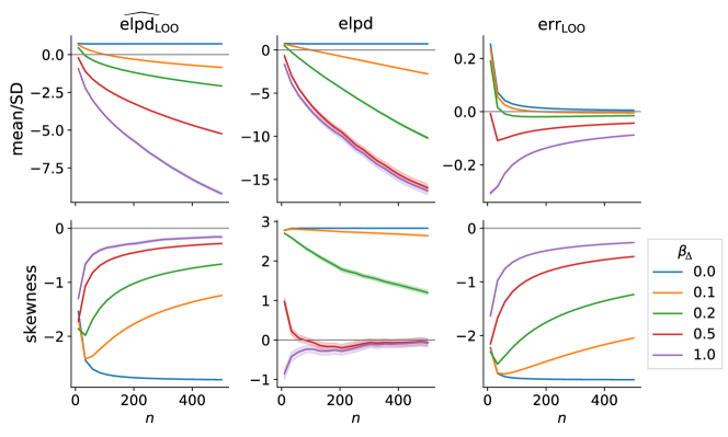
Figure 11: Illustration of the mean relative to the standard deviation and skewness for ${\widehat{\mathrm{elpd}}_{\mathrm{\scriptscriptstyle LOO}}\bigr{(}{\mathrm{M_{A},M_{B}}}\mid y\bigl{)}}$, ${\mathrm{elpd}\bigr{(}{\mathrm{M_{A},M_{B}}}\mid y\bigl{)}}$, and for the error ${\mathrm{err}_{\mathrm{\scriptscriptstyle LOO}}\bigr{(}{\mathrm{M_{A},M_{B}}}\mid y\bigl{)}}$ as a function of the data size $n$. The data consist of an intercept and two covariates following standard normal distribution. One of the covariates with true effect $\beta_{\Delta}$ is considered only in model ${\mathrm{M}_{b}}$. The solid lines corresponds to the median over a Bayesian bootstrap sample of size 2000 from 2000 simulated $X$s. Although wide enough to be visible only in some lines in the middle column, a shaded area around the lines illustrates the 95 % confidence interval.

D.6 One Covariate Case

Let us inspect the behaviour of the moments $m_{1}$, $\overline{m}_{2}$, and $\tilde{m}_{3}$ of the LOO-CV error formulated in Appendix D.3 in a nested example case, where a null model is compared to a model with one covariate. Consider that $n$ is even, $n\geq 4$, and $d=2$ so that $X$ is two dimensional. One column in $X$ corresponds to the intercept, being full of $1$s, and the other column corresponds to the covariate, consisting of half $1$s and $-1$s in any order. Model $\mathrm{M_{A}}$ only considers the intercept column and model $\mathrm{M_{B}}$ considers both the intercept and the sole covariate column.

In addition, we set the data generating mechanism parameters $\Sigma_{\star}$ and $\mu_{\star,\,i}$ to the following form, in which the observations are independent and there is one outlier observation with some index $i_{\text{out}}$ for which $x_{i_{\text{out}}}=1$:

$$\Sigma_{\star} =s_{\star}^{2}\,\mathrm{I}_{n},$$ (215)

$$\mu_{\star,\,i} =\begin{cases}m_{\star}&\text{when }i=i_{\text{out}}\,,\\ 0&\text{otherwise}.\end{cases}$$ (216)

Let $\mathbbm{1}_{n}$ and $0_{n}$ denote a vector of ones and zeroes of length $n$ respectively. Let vector $x\in\mathbb{R}^{n}$ denote the covariate column in $X$. Considering the half $1$s half $-1$s structure of $x$ yields

$$x_{i}^{2} =1,$$ (217)

$$x^{\mathchoice{\raisebox{2.6pt}{$\scriptstyle\mathrm{T}$}}{\raisebox{2.6pt}{$\scriptstyle\mathrm{T}$}}{\raisebox{1.0pt}{$\scriptscriptstyle\mathrm{T}$}}{\raisebox{0.5pt}{\tiny$\scriptscriptstyle\mathrm{T}$}}}x =n,$$ (218)

$$\mathbbm{1}_{n}^{\mathchoice{\raisebox{2.6pt}{$\scriptstyle\mathrm{T}$}}{\raisebox{2.6pt}{$\scriptstyle\mathrm{T}$}}{\raisebox{1.0pt}{$\scriptscriptstyle\mathrm{T}$}}{\raisebox{0.5pt}{\tiny$\scriptscriptstyle\mathrm{T}$}}}x =0,$$ (219)

$$x_{-i}^{\mathchoice{\raisebox{2.6pt}{$\scriptstyle\mathrm{T}$}}{\raisebox{2.6pt}{$\scriptstyle\mathrm{T}$}}{\raisebox{1.0pt}{$\scriptscriptstyle\mathrm{T}$}}{\raisebox{0.5pt}{\tiny$\scriptscriptstyle\mathrm{T}$}}}x_{-i} =n-1,$$ (220)

$$\mathbbm{1}_{n-1}^{\mathchoice{\raisebox{2.6pt}{$\scriptstyle\mathrm{T}$}}{\raisebox{2.6pt}{$\scriptstyle\mathrm{T}$}}{\raisebox{1.0pt}{$\scriptscriptstyle\mathrm{T}$}}{\raisebox{0.5pt}{\tiny$\scriptscriptstyle\mathrm{T}$}}}x_{-i} =-x_{i},$$ (221)

$$(x_{i}x_{j}+1)^{2} =2(x_{i}x_{j}+1),$$ (222)

$$\operatorname{diag}(xx^{\mathchoice{\raisebox{2.6pt}{$\scriptstyle\mathrm{T}$}}{\raisebox{2.6pt}{$\scriptstyle\mathrm{T}$}}{\raisebox{1.0pt}{$\scriptscriptstyle\mathrm{T}$}}{\raisebox{0.5pt}{\tiny$\scriptscriptstyle\mathrm{T}$}}})=\mathbbm{1}_{n},$$ (223)

for all $i,j=1,2,\dots,n$. Let $\beta_{1}$ denote the true covariate effect included in vector $\beta$. As can be seen from the equations of the parameters of the LOO-CV error, the effects in $\beta$, which are considered by both models, do not affect the outcome. In this problem setting, the intercept coefficient is one such an effect. The parameters $\hat{y}_{-{\mathrm{A}}}$ and $\hat{y}_{-{\mathrm{B}}}$ defined in equation (87), which are involved in the formulation of the LOO-CV error, simplifies to

$$\hat{y}_{-{\mathrm{A}}} =X_{[\boldsymbol{\cdot},-{\mathrm{A}}]}\beta_{-{\mathrm{A}}}=\beta_{1}x$$ (224)

$$\hat{y}_{-{\mathrm{B}}} =X_{[\boldsymbol{\cdot},-{\mathrm{B}}]}\beta_{-{\mathrm{B}}}=0_{n}\,.$$ (225)

D.6.1 Elpd

In this section, we derive simplified analytic form for ${\mathrm{elpd}\bigr{(}{\mathrm{M_{A},M_{B}}}\mid y\bigl{)}}$ presented in Appendix D.1.2 and for some moments of interest in the one covariate case defined in Appendix D.6. First we derive the parameters $A_{\mathrm{A-B}}$, $b_{\mathrm{A-B}}$, and $c_{\mathrm{A-B}}$ defined in Appendix D.1.2 and then we use them to derive the respective moments of interest defined in Appendix D.5.

Parameters

Following the notation in Appendix D.1, in the one covariate case defined in Appendix D.6, let us find simplified form for the matrices $P_{k}$, $D_{k}$, and for the required products for the LOO-CV error parameters

$$P_{k}D_{k},$$

$$P_{k}D_{k}P_{k},$$

$$P_{k}D_{k}\mathopen{}\mathclose{{}\left(P_{k}-\mathrm{I}}\right),$$

$$\mathopen{}\mathclose{{}\left(P_{k}-\mathrm{I}}\right)D_{k}\mathopen{}\mathclose{{}\left(P_{k}-\mathrm{I}}\right),$$

$$\mathopen{}\mathclose{{}\left(P_{k}-\mathrm{I}}\right)D_{k},$$

$$D_{\mathrm{A}}-D_{\mathrm{B}}$$ (226)

for ${\mathrm{M}_{k}}\in\{{\mathrm{A}},{\mathrm{B}}\}$, presented in Appendix D.3. For model $\mathrm{M_{A}}$ we have

$$P_{\mathrm{A}} =X_{[\boldsymbol{\cdot},{\mathrm{A}}]}\mathopen{}\mathclose{{}\left(X_{[\boldsymbol{\cdot},{\mathrm{A}}]}^{\mathchoice{\raisebox{2.6pt}{$\scriptstyle\mathrm{T}$}}{\raisebox{2.6pt}{$\scriptstyle\mathrm{T}$}}{\raisebox{1.0pt}{$\scriptscriptstyle\mathrm{T}$}}{\raisebox{0.5pt}{\tiny$\scriptscriptstyle\mathrm{T}$}}}X_{[\boldsymbol{\cdot},{\mathrm{A}}]}}\right)^{-1}X_{[\boldsymbol{\cdot},{\mathrm{A}}]}^{\mathchoice{\raisebox{2.6pt}{$\scriptstyle\mathrm{T}$}}{\raisebox{2.6pt}{$\scriptstyle\mathrm{T}$}}{\raisebox{1.0pt}{$\scriptscriptstyle\mathrm{T}$}}{\raisebox{0.5pt}{\tiny$\scriptscriptstyle\mathrm{T}$}}}$$

$$=\mathbbm{1}_{n}\mathopen{}\mathclose{{}\left(\mathbbm{1}_{n}^{\mathchoice{\raisebox{2.6pt}{$\scriptstyle\mathrm{T}$}}{\raisebox{2.6pt}{$\scriptstyle\mathrm{T}$}}{\raisebox{1.0pt}{$\scriptscriptstyle\mathrm{T}$}}{\raisebox{0.5pt}{\tiny$\scriptscriptstyle\mathrm{T}$}}}\mathbbm{1}_{n}}\right)^{-1}\mathbbm{1}_{n}^{\mathchoice{\raisebox{2.6pt}{$\scriptstyle\mathrm{T}$}}{\raisebox{2.6pt}{$\scriptstyle\mathrm{T}$}}{\raisebox{1.0pt}{$\scriptscriptstyle\mathrm{T}$}}{\raisebox{0.5pt}{\tiny$\scriptscriptstyle\mathrm{T}$}}}$$

$$=\frac{1}{n}\mathbbm{1}_{n}\mathbbm{1}_{n}^{\mathchoice{\raisebox{2.6pt}{$\scriptstyle\mathrm{T}$}}{\raisebox{2.6pt}{$\scriptstyle\mathrm{T}$}}{\raisebox{1.0pt}{$\scriptscriptstyle\mathrm{T}$}}{\raisebox{0.5pt}{\tiny$\scriptscriptstyle\mathrm{T}$}}}$$ (227)

and

$$D_{\mathrm{A}} =\mathopen{}\mathclose{{}\left(\mathopen{}\mathclose{{}\left(P_{{\mathrm{A}}}\odot\mathrm{I}_{n}}\right)+\mathrm{I}_{n}}\right)^{-1}$$

$$=\frac{n}{n+1}\mathrm{I}_{n}\,.$$ (228)

Now we get

$$P_{\mathrm{A}}D_{\mathrm{A}} =\frac{n}{n+1}\frac{1}{n}\mathbbm{1}_{n}\mathbbm{1}_{n}^{\mathchoice{\raisebox{2.6pt}{$\scriptstyle\mathrm{T}$}}{\raisebox{2.6pt}{$\scriptstyle\mathrm{T}$}}{\raisebox{1.0pt}{$\scriptscriptstyle\mathrm{T}$}}{\raisebox{0.5pt}{\tiny$\scriptscriptstyle\mathrm{T}$}}}\mathrm{I}_{n}$$

$$=\frac{1}{n+1}\mathbbm{1}_{n}\mathbbm{1}_{n}^{\mathchoice{\raisebox{2.6pt}{$\scriptstyle\mathrm{T}$}}{\raisebox{2.6pt}{$\scriptstyle\mathrm{T}$}}{\raisebox{1.0pt}{$\scriptscriptstyle\mathrm{T}$}}{\raisebox{0.5pt}{\tiny$\scriptscriptstyle\mathrm{T}$}}}\,,$$ (229)

$$P_{\mathrm{A}}D_{\mathrm{A}}P_{\mathrm{A}} =\frac{n}{n+1}\underbrace{P_{\mathrm{A}}\mathrm{I}_{n}P_{\mathrm{A}}}_{=P_{\mathrm{A}}}$$

$$=\frac{1}{n+1}\mathbbm{1}_{n}\mathbbm{1}_{n}^{\mathchoice{\raisebox{2.6pt}{$\scriptstyle\mathrm{T}$}}{\raisebox{2.6pt}{$\scriptstyle\mathrm{T}$}}{\raisebox{1.0pt}{$\scriptscriptstyle\mathrm{T}$}}{\raisebox{0.5pt}{\tiny$\scriptscriptstyle\mathrm{T}$}}}\,,$$ (230)

$$P_{\mathrm{A}}D_{\mathrm{A}}\mathopen{}\mathclose{{}\left(P_{\mathrm{A}}-\mathrm{I}}\right) =P_{\mathrm{A}}D_{\mathrm{A}}P_{\mathrm{A}}-P_{\mathrm{A}}D_{\mathrm{A}}$$

$$=0\,,$$ (231)

$$\mathopen{}\mathclose{{}\left(P_{\mathrm{A}}-\mathrm{I}}\right)D_{\mathrm{A}}\mathopen{}\mathclose{{}\left(P_{\mathrm{A}}-\mathrm{I}}\right) =P_{\mathrm{A}}D_{\mathrm{A}}P_{\mathrm{A}}-P_{\mathrm{A}}D_{\mathrm{A}}-D_{\mathrm{A}}P_{\mathrm{A}}+D_{\mathrm{A}}$$

$$=\frac{n}{n+1}\mathrm{I}_{n}-\frac{1}{n+1}\mathbbm{1}_{n}\mathbbm{1}_{n}^{\mathchoice{\raisebox{2.6pt}{$\scriptstyle\mathrm{T}$}}{\raisebox{2.6pt}{$\scriptstyle\mathrm{T}$}}{\raisebox{1.0pt}{$\scriptscriptstyle\mathrm{T}$}}{\raisebox{0.5pt}{\tiny$\scriptscriptstyle\mathrm{T}$}}}\,,$$ (232)

$$\mathopen{}\mathclose{{}\left(P_{\mathrm{A}}-\mathrm{I}}\right)D_{\mathrm{A}} =D_{\mathrm{A}}P_{\mathrm{A}}-D_{\mathrm{A}}$$

$$=-\frac{n}{n+1}\mathrm{I}_{n}+\frac{1}{n+1}\mathbbm{1}_{n}\mathbbm{1}_{n}^{\mathchoice{\raisebox{2.6pt}{$\scriptstyle\mathrm{T}$}}{\raisebox{2.6pt}{$\scriptstyle\mathrm{T}$}}{\raisebox{1.0pt}{$\scriptscriptstyle\mathrm{T}$}}{\raisebox{0.5pt}{\tiny$\scriptscriptstyle\mathrm{T}$}}}\,.$$ (233)

For model $\mathrm{M_{B}}$ we have

$$P_{\mathrm{B}} =X_{[\boldsymbol{\cdot},{\mathrm{B}}]}\mathopen{}\mathclose{{}\left((X_{[\boldsymbol{\cdot},{\mathrm{B}}]}^{\mathchoice{\raisebox{2.6pt}{$\scriptstyle\mathrm{T}$}}{\raisebox{2.6pt}{$\scriptstyle\mathrm{T}$}}{\raisebox{1.0pt}{$\scriptscriptstyle\mathrm{T}$}}{\raisebox{0.5pt}{\tiny$\scriptscriptstyle\mathrm{T}$}}}X_{[\boldsymbol{\cdot},{\mathrm{B}}]}}\right)^{-1}X_{[\boldsymbol{\cdot},{\mathrm{B}}]}^{\mathchoice{\raisebox{2.6pt}{$\scriptstyle\mathrm{T}$}}{\raisebox{2.6pt}{$\scriptstyle\mathrm{T}$}}{\raisebox{1.0pt}{$\scriptscriptstyle\mathrm{T}$}}{\raisebox{0.5pt}{\tiny$\scriptscriptstyle\mathrm{T}$}}},$$

$$=\begin{bmatrix}\mathbbm{1}_{n}&x\end{bmatrix}\mathopen{}\mathclose{{}\left(\begin{bmatrix}\mathbbm{1}_{n}&x\end{bmatrix}^{\mathchoice{\raisebox{2.6pt}{$\scriptstyle\mathrm{T}$}}{\raisebox{2.6pt}{$\scriptstyle\mathrm{T}$}}{\raisebox{1.0pt}{$\scriptscriptstyle\mathrm{T}$}}{\raisebox{0.5pt}{\tiny$\scriptscriptstyle\mathrm{T}$}}}\begin{bmatrix}\mathbbm{1}_{n}&x\end{bmatrix}}\right)^{-1}\begin{bmatrix}\mathbbm{1}_{n}&x\end{bmatrix}^{\mathchoice{\raisebox{2.6pt}{$\scriptstyle\mathrm{T}$}}{\raisebox{2.6pt}{$\scriptstyle\mathrm{T}$}}{\raisebox{1.0pt}{$\scriptscriptstyle\mathrm{T}$}}{\raisebox{0.5pt}{\tiny$\scriptscriptstyle\mathrm{T}$}}}$$

$$=\begin{bmatrix}\mathbbm{1}_{n}&x\end{bmatrix}\begin{bmatrix}\mathbbm{1}_{n}^{\mathchoice{\raisebox{2.6pt}{$\scriptstyle\mathrm{T}$}}{\raisebox{2.6pt}{$\scriptstyle\mathrm{T}$}}{\raisebox{1.0pt}{$\scriptscriptstyle\mathrm{T}$}}{\raisebox{0.5pt}{\tiny$\scriptscriptstyle\mathrm{T}$}}}\mathbbm{1}_{n}&\mathbbm{1}_{n}^{\mathchoice{\raisebox{2.6pt}{$\scriptstyle\mathrm{T}$}}{\raisebox{2.6pt}{$\scriptstyle\mathrm{T}$}}{\raisebox{1.0pt}{$\scriptscriptstyle\mathrm{T}$}}{\raisebox{0.5pt}{\tiny$\scriptscriptstyle\mathrm{T}$}}}x\\ \mathbbm{1}_{n}^{\mathchoice{\raisebox{2.6pt}{$\scriptstyle\mathrm{T}$}}{\raisebox{2.6pt}{$\scriptstyle\mathrm{T}$}}{\raisebox{1.0pt}{$\scriptscriptstyle\mathrm{T}$}}{\raisebox{0.5pt}{\tiny$\scriptscriptstyle\mathrm{T}$}}}x&x^{\mathchoice{\raisebox{2.6pt}{$\scriptstyle\mathrm{T}$}}{\raisebox{2.6pt}{$\scriptstyle\mathrm{T}$}}{\raisebox{1.0pt}{$\scriptscriptstyle\mathrm{T}$}}{\raisebox{0.5pt}{\tiny$\scriptscriptstyle\mathrm{T}$}}}x\end{bmatrix}^{-1}\begin{bmatrix}\mathbbm{1}_{n}&x\end{bmatrix}^{\mathchoice{\raisebox{2.6pt}{$\scriptstyle\mathrm{T}$}}{\raisebox{2.6pt}{$\scriptstyle\mathrm{T}$}}{\raisebox{1.0pt}{$\scriptscriptstyle\mathrm{T}$}}{\raisebox{0.5pt}{\tiny$\scriptscriptstyle\mathrm{T}$}}}$$

$$=\begin{bmatrix}\mathbbm{1}_{n}&x\end{bmatrix}\begin{bmatrix}n&0\\ 0&n\end{bmatrix}^{-1}\begin{bmatrix}\mathbbm{1}_{n}&x\end{bmatrix}^{\mathchoice{\raisebox{2.6pt}{$\scriptstyle\mathrm{T}$}}{\raisebox{2.6pt}{$\scriptstyle\mathrm{T}$}}{\raisebox{1.0pt}{$\scriptscriptstyle\mathrm{T}$}}{\raisebox{0.5pt}{\tiny$\scriptscriptstyle\mathrm{T}$}}}$$

$$=\frac{1}{n^{2}}\begin{bmatrix}\mathbbm{1}_{n}&x\end{bmatrix}\begin{bmatrix}n&0\\ 0&n\end{bmatrix}\begin{bmatrix}\mathbbm{1}_{n}&x\end{bmatrix}^{\mathchoice{\raisebox{2.6pt}{$\scriptstyle\mathrm{T}$}}{\raisebox{2.6pt}{$\scriptstyle\mathrm{T}$}}{\raisebox{1.0pt}{$\scriptscriptstyle\mathrm{T}$}}{\raisebox{0.5pt}{\tiny$\scriptscriptstyle\mathrm{T}$}}}$$

$$=\frac{1}{n}\mathopen{}\mathclose{{}\left(\mathbbm{1}_{n}\mathbbm{1}_{n}^{\mathchoice{\raisebox{2.6pt}{$\scriptstyle\mathrm{T}$}}{\raisebox{2.6pt}{$\scriptstyle\mathrm{T}$}}{\raisebox{1.0pt}{$\scriptscriptstyle\mathrm{T}$}}{\raisebox{0.5pt}{\tiny$\scriptscriptstyle\mathrm{T}$}}}+xx^{\mathchoice{\raisebox{2.6pt}{$\scriptstyle\mathrm{T}$}}{\raisebox{2.6pt}{$\scriptstyle\mathrm{T}$}}{\raisebox{1.0pt}{$\scriptscriptstyle\mathrm{T}$}}{\raisebox{0.5pt}{\tiny$\scriptscriptstyle\mathrm{T}$}}}}\right)$$ (234)

and

$$D_{\mathrm{B}} =\mathopen{}\mathclose{{}\left(\mathopen{}\mathclose{{}\left(P_{{\mathrm{B}}}\odot\mathrm{I}_{n}}\right)+\mathrm{I}_{n}}\right)^{-1}$$

$$=\mathopen{}\mathclose{{}\left(\frac{1}{n}\mathopen{}\mathclose{{}\left(\mathrm{I}_{n}+\mathrm{I}_{n}}\right)+\mathrm{I}_{n}}\right)^{-1}$$

$$=\frac{n}{n+2}\mathrm{I}_{n}\,.$$ (235)

Now we get

$$P_{\mathrm{B}}D_{\mathrm{B}} =\frac{1}{n}\frac{n}{n+2}\mathopen{}\mathclose{{}\left(\mathbbm{1}_{n}\mathbbm{1}_{n}^{\mathchoice{\raisebox{2.6pt}{$\scriptstyle\mathrm{T}$}}{\raisebox{2.6pt}{$\scriptstyle\mathrm{T}$}}{\raisebox{1.0pt}{$\scriptscriptstyle\mathrm{T}$}}{\raisebox{0.5pt}{\tiny$\scriptscriptstyle\mathrm{T}$}}}+xx^{\mathchoice{\raisebox{2.6pt}{$\scriptstyle\mathrm{T}$}}{\raisebox{2.6pt}{$\scriptstyle\mathrm{T}$}}{\raisebox{1.0pt}{$\scriptscriptstyle\mathrm{T}$}}{\raisebox{0.5pt}{\tiny$\scriptscriptstyle\mathrm{T}$}}}}\right)\mathrm{I}_{n}$$

$$=\frac{1}{n+2}\mathopen{}\mathclose{{}\left(\mathbbm{1}_{n}\mathbbm{1}_{n}^{\mathchoice{\raisebox{2.6pt}{$\scriptstyle\mathrm{T}$}}{\raisebox{2.6pt}{$\scriptstyle\mathrm{T}$}}{\raisebox{1.0pt}{$\scriptscriptstyle\mathrm{T}$}}{\raisebox{0.5pt}{\tiny$\scriptscriptstyle\mathrm{T}$}}}+xx^{\mathchoice{\raisebox{2.6pt}{$\scriptstyle\mathrm{T}$}}{\raisebox{2.6pt}{$\scriptstyle\mathrm{T}$}}{\raisebox{1.0pt}{$\scriptscriptstyle\mathrm{T}$}}{\raisebox{0.5pt}{\tiny$\scriptscriptstyle\mathrm{T}$}}}}\right)\,,$$ (236)

$$P_{\mathrm{B}}D_{\mathrm{B}}P_{\mathrm{B}} =\frac{n}{n+2}\underbrace{P_{\mathrm{B}}\mathrm{I}_{n}P_{\mathrm{B}}}_{=P_{\mathrm{B}}}$$

$$=\frac{1}{n+2}\mathopen{}\mathclose{{}\left(\mathbbm{1}_{n}\mathbbm{1}_{n}^{\mathchoice{\raisebox{2.6pt}{$\scriptstyle\mathrm{T}$}}{\raisebox{2.6pt}{$\scriptstyle\mathrm{T}$}}{\raisebox{1.0pt}{$\scriptscriptstyle\mathrm{T}$}}{\raisebox{0.5pt}{\tiny$\scriptscriptstyle\mathrm{T}$}}}+xx^{\mathchoice{\raisebox{2.6pt}{$\scriptstyle\mathrm{T}$}}{\raisebox{2.6pt}{$\scriptstyle\mathrm{T}$}}{\raisebox{1.0pt}{$\scriptscriptstyle\mathrm{T}$}}{\raisebox{0.5pt}{\tiny$\scriptscriptstyle\mathrm{T}$}}}}\right)\,,$$ (237)

$$P_{\mathrm{B}}D_{\mathrm{B}}\mathopen{}\mathclose{{}\left(P_{\mathrm{B}}-\mathrm{I}}\right) =P_{\mathrm{B}}D_{\mathrm{B}}P_{\mathrm{B}}-P_{\mathrm{B}}D_{\mathrm{B}}$$

$$=0\,,$$ (238)

$$\mathopen{}\mathclose{{}\left(P_{\mathrm{B}}-\mathrm{I}}\right)D_{\mathrm{B}}\mathopen{}\mathclose{{}\left(P_{\mathrm{B}}-\mathrm{I}}\right) =P_{\mathrm{B}}D_{\mathrm{B}}P_{\mathrm{B}}-P_{\mathrm{B}}D_{\mathrm{B}}-D_{\mathrm{B}}P_{\mathrm{B}}+D_{\mathrm{B}}$$

$$=\frac{n}{n+2}\mathrm{I}_{n}-\frac{1}{n+2}\mathopen{}\mathclose{{}\left(\mathbbm{1}_{n}\mathbbm{1}_{n}^{\mathchoice{\raisebox{2.6pt}{$\scriptstyle\mathrm{T}$}}{\raisebox{2.6pt}{$\scriptstyle\mathrm{T}$}}{\raisebox{1.0pt}{$\scriptscriptstyle\mathrm{T}$}}{\raisebox{0.5pt}{\tiny$\scriptscriptstyle\mathrm{T}$}}}+xx^{\mathchoice{\raisebox{2.6pt}{$\scriptstyle\mathrm{T}$}}{\raisebox{2.6pt}{$\scriptstyle\mathrm{T}$}}{\raisebox{1.0pt}{$\scriptscriptstyle\mathrm{T}$}}{\raisebox{0.5pt}{\tiny$\scriptscriptstyle\mathrm{T}$}}}}\right)\,,$$ (239)

$$\mathopen{}\mathclose{{}\left(P_{\mathrm{B}}-\mathrm{I}}\right)D_{\mathrm{B}} =D_{\mathrm{B}}P_{\mathrm{B}}-D_{\mathrm{B}}$$

$$=-\frac{n}{n+2}\mathrm{I}_{n}+\frac{1}{n+2}\mathopen{}\mathclose{{}\left(\mathbbm{1}_{n}\mathbbm{1}_{n}^{\mathchoice{\raisebox{2.6pt}{$\scriptstyle\mathrm{T}$}}{\raisebox{2.6pt}{$\scriptstyle\mathrm{T}$}}{\raisebox{1.0pt}{$\scriptscriptstyle\mathrm{T}$}}{\raisebox{0.5pt}{\tiny$\scriptscriptstyle\mathrm{T}$}}}+xx^{\mathchoice{\raisebox{2.6pt}{$\scriptstyle\mathrm{T}$}}{\raisebox{2.6pt}{$\scriptstyle\mathrm{T}$}}{\raisebox{1.0pt}{$\scriptscriptstyle\mathrm{T}$}}{\raisebox{0.5pt}{\tiny$\scriptscriptstyle\mathrm{T}$}}}}\right)\,.$$ (240)

Furthermore, we get

$$D_{\mathrm{A}}-D_{\mathrm{B}} =\frac{n}{n+1}\mathrm{I}_{n}-\frac{n}{n+2}\mathrm{I}_{n}=\frac{n}{(n+1)(n+2)}\mathrm{I}_{n}\,.$$ (241)

Moreover, we get

$$B_{{\mathrm{A}},1} =-P_{{\mathrm{A}}}D_{{\mathrm{A}}}\mathopen{}\mathclose{{}\left(P_{{\mathrm{A}}}-\mathrm{I}}\right)$$

$$=0\,,$$ (242)

$$B_{{\mathrm{B}},1} =-P_{{\mathrm{B}}}D_{{\mathrm{B}}}\mathopen{}\mathclose{{}\left(P_{{\mathrm{B}}}-\mathrm{I}}\right)$$

$$=0\,,$$ (243)

$$C_{{\mathrm{A}},1} =-\frac{1}{2}\mathopen{}\mathclose{{}\left(P_{{\mathrm{A}}}-\mathrm{I}}\right)D_{{\mathrm{A}}}\mathopen{}\mathclose{{}\left(P_{{\mathrm{A}}}-\mathrm{I}}\right)$$

$$=-\frac{n}{2(n+1)}\mathrm{I}_{n}+\frac{1}{2(n+1)}\mathbbm{1}_{n}\mathbbm{1}_{n}^{\mathchoice{\raisebox{2.6pt}{$\scriptstyle\mathrm{T}$}}{\raisebox{2.6pt}{$\scriptstyle\mathrm{T}$}}{\raisebox{1.0pt}{$\scriptscriptstyle\mathrm{T}$}}{\raisebox{0.5pt}{\tiny$\scriptscriptstyle\mathrm{T}$}}}\,,$$ (244)

$$C_{{\mathrm{B}},1} =-\frac{1}{2}\mathopen{}\mathclose{{}\left(P_{{\mathrm{B}}}-\mathrm{I}}\right)D_{{\mathrm{B}}}\mathopen{}\mathclose{{}\left(P_{{\mathrm{B}}}-\mathrm{I}}\right)$$

$$=-\frac{n}{2(n+2)}\mathrm{I}_{n}+\frac{1}{2(n+2)}\mathopen{}\mathclose{{}\left(\mathbbm{1}_{n}\mathbbm{1}_{n}^{\mathchoice{\raisebox{2.6pt}{$\scriptstyle\mathrm{T}$}}{\raisebox{2.6pt}{$\scriptstyle\mathrm{T}$}}{\raisebox{1.0pt}{$\scriptscriptstyle\mathrm{T}$}}{\raisebox{0.5pt}{\tiny$\scriptscriptstyle\mathrm{T}$}}}+xx^{\mathchoice{\raisebox{2.6pt}{$\scriptstyle\mathrm{T}$}}{\raisebox{2.6pt}{$\scriptstyle\mathrm{T}$}}{\raisebox{1.0pt}{$\scriptscriptstyle\mathrm{T}$}}{\raisebox{0.5pt}{\tiny$\scriptscriptstyle\mathrm{T}$}}}}\right)\,,$$ (245)

$$C_{{\mathrm{A}},2} =\mathopen{}\mathclose{{}\left(P_{{\mathrm{A}}}-\mathrm{I}}\right)D_{{\mathrm{A}}}$$

$$=-\frac{n}{n+1}\mathrm{I}_{n}+\frac{1}{n+1}\mathbbm{1}_{n}\mathbbm{1}_{n}^{\mathchoice{\raisebox{2.6pt}{$\scriptstyle\mathrm{T}$}}{\raisebox{2.6pt}{$\scriptstyle\mathrm{T}$}}{\raisebox{1.0pt}{$\scriptscriptstyle\mathrm{T}$}}{\raisebox{0.5pt}{\tiny$\scriptscriptstyle\mathrm{T}$}}}$$ (246)

$$C_{{\mathrm{B}},2} =\mathopen{}\mathclose{{}\left(P_{{\mathrm{B}}}-\mathrm{I}}\right)D_{{\mathrm{B}}}$$

$$=-\frac{n}{n+2}\mathrm{I}_{n}+\frac{1}{n+2}\mathopen{}\mathclose{{}\left(\mathbbm{1}_{n}\mathbbm{1}_{n}^{\mathchoice{\raisebox{2.6pt}{$\scriptstyle\mathrm{T}$}}{\raisebox{2.6pt}{$\scriptstyle\mathrm{T}$}}{\raisebox{1.0pt}{$\scriptscriptstyle\mathrm{T}$}}{\raisebox{0.5pt}{\tiny$\scriptscriptstyle\mathrm{T}$}}}+xx^{\mathchoice{\raisebox{2.6pt}{$\scriptstyle\mathrm{T}$}}{\raisebox{2.6pt}{$\scriptstyle\mathrm{T}$}}{\raisebox{1.0pt}{$\scriptscriptstyle\mathrm{T}$}}{\raisebox{0.5pt}{\tiny$\scriptscriptstyle\mathrm{T}$}}}}\right)\,,$$ (247)

and

$$A_{{\mathrm{A-B}},1} =-\frac{1}{2}\mathopen{}\mathclose{{}\left(P_{{\mathrm{A}}}D_{{\mathrm{A}}}P_{{\mathrm{A}}}-P_{{\mathrm{B}}}D_{{\mathrm{B}}}P_{{\mathrm{B}}}}\right)$$

$$=-\frac{1}{2}\mathopen{}\mathclose{{}\left(\frac{1}{n+1}\mathbbm{1}_{n}\mathbbm{1}_{n}^{\mathchoice{\raisebox{2.6pt}{$\scriptstyle\mathrm{T}$}}{\raisebox{2.6pt}{$\scriptstyle\mathrm{T}$}}{\raisebox{1.0pt}{$\scriptscriptstyle\mathrm{T}$}}{\raisebox{0.5pt}{\tiny$\scriptscriptstyle\mathrm{T}$}}}-\frac{1}{n+2}\mathopen{}\mathclose{{}\left(\mathbbm{1}_{n}\mathbbm{1}_{n}^{\mathchoice{\raisebox{2.6pt}{$\scriptstyle\mathrm{T}$}}{\raisebox{2.6pt}{$\scriptstyle\mathrm{T}$}}{\raisebox{1.0pt}{$\scriptscriptstyle\mathrm{T}$}}{\raisebox{0.5pt}{\tiny$\scriptscriptstyle\mathrm{T}$}}}+xx^{\mathchoice{\raisebox{2.6pt}{$\scriptstyle\mathrm{T}$}}{\raisebox{2.6pt}{$\scriptstyle\mathrm{T}$}}{\raisebox{1.0pt}{$\scriptscriptstyle\mathrm{T}$}}{\raisebox{0.5pt}{\tiny$\scriptscriptstyle\mathrm{T}$}}}}\right)}\right)$$

$$=-\frac{1}{2(n+1)(n+2)}\mathbbm{1}_{n}\mathbbm{1}_{n}^{\mathchoice{\raisebox{2.6pt}{$\scriptstyle\mathrm{T}$}}{\raisebox{2.6pt}{$\scriptstyle\mathrm{T}$}}{\raisebox{1.0pt}{$\scriptscriptstyle\mathrm{T}$}}{\raisebox{0.5pt}{\tiny$\scriptscriptstyle\mathrm{T}$}}}+\frac{1}{2(n+2)}xx^{\mathchoice{\raisebox{2.6pt}{$\scriptstyle\mathrm{T}$}}{\raisebox{2.6pt}{$\scriptstyle\mathrm{T}$}}{\raisebox{1.0pt}{$\scriptscriptstyle\mathrm{T}$}}{\raisebox{0.5pt}{\tiny$\scriptscriptstyle\mathrm{T}$}}}\,,$$ (248)

$$B_{{\mathrm{A-B}},2} =P_{{\mathrm{A}}}D_{{\mathrm{A}}}-P_{{\mathrm{B}}}D_{{\mathrm{B}}}$$

$$=\frac{1}{n+1}\mathbbm{1}_{n}\mathbbm{1}_{n}^{\mathchoice{\raisebox{2.6pt}{$\scriptstyle\mathrm{T}$}}{\raisebox{2.6pt}{$\scriptstyle\mathrm{T}$}}{\raisebox{1.0pt}{$\scriptscriptstyle\mathrm{T}$}}{\raisebox{0.5pt}{\tiny$\scriptscriptstyle\mathrm{T}$}}}-\frac{1}{n+2}\mathopen{}\mathclose{{}\left(\mathbbm{1}_{n}\mathbbm{1}_{n}^{\mathchoice{\raisebox{2.6pt}{$\scriptstyle\mathrm{T}$}}{\raisebox{2.6pt}{$\scriptstyle\mathrm{T}$}}{\raisebox{1.0pt}{$\scriptscriptstyle\mathrm{T}$}}{\raisebox{0.5pt}{\tiny$\scriptscriptstyle\mathrm{T}$}}}+xx^{\mathchoice{\raisebox{2.6pt}{$\scriptstyle\mathrm{T}$}}{\raisebox{2.6pt}{$\scriptstyle\mathrm{T}$}}{\raisebox{1.0pt}{$\scriptscriptstyle\mathrm{T}$}}{\raisebox{0.5pt}{\tiny$\scriptscriptstyle\mathrm{T}$}}}}\right)$$

$$=\frac{1}{(n+2)(n+1)}\mathbbm{1}_{n}\mathbbm{1}_{n}^{\mathchoice{\raisebox{2.6pt}{$\scriptstyle\mathrm{T}$}}{\raisebox{2.6pt}{$\scriptstyle\mathrm{T}$}}{\raisebox{1.0pt}{$\scriptscriptstyle\mathrm{T}$}}{\raisebox{0.5pt}{\tiny$\scriptscriptstyle\mathrm{T}$}}}-\frac{1}{n+2}xx^{\mathchoice{\raisebox{2.6pt}{$\scriptstyle\mathrm{T}$}}{\raisebox{2.6pt}{$\scriptstyle\mathrm{T}$}}{\raisebox{1.0pt}{$\scriptscriptstyle\mathrm{T}$}}{\raisebox{0.5pt}{\tiny$\scriptscriptstyle\mathrm{T}$}}}\,,$$ (249)

$$C_{{\mathrm{A-B}},3} =-\frac{1}{2}\mathopen{}\mathclose{{}\left(D_{{\mathrm{A}}}-D_{{\mathrm{B}}}}\right)$$

$$=-\frac{n}{2(n+1)(n+2)}\mathrm{I}_{n}\,,$$ (250)

$$c_{{\mathrm{A-B}},4} =\frac{1}{2}\log\mathopen{}\mathclose{{}\left(\prod_{i=1}^{n}\frac{D_{{\mathrm{A}},[i,i]}}{D_{{\mathrm{B}},[i,i]}}}\right)$$

$$=\frac{1}{2}\log\mathopen{}\mathclose{{}\left(\prod_{i=1}^{n}\frac{\frac{n}{n+1}}{\frac{n}{n+2}}}\right)$$

$$=\frac{n}{2}\log\frac{n+2}{n+1}\,.$$ (251)

Now we get

$$A_{\mathrm{A-B}} =\frac{1}{\tau^{2}}A_{{\mathrm{A-B}},1}$$

$$=\frac{1}{\tau^{2}}\mathopen{}\mathclose{{}\left(-\frac{1}{2(n+1)(n+2)}\mathbbm{1}_{n}\mathbbm{1}_{n}^{\mathchoice{\raisebox{2.6pt}{$\scriptstyle\mathrm{T}$}}{\raisebox{2.6pt}{$\scriptstyle\mathrm{T}$}}{\raisebox{1.0pt}{$\scriptscriptstyle\mathrm{T}$}}{\raisebox{0.5pt}{\tiny$\scriptscriptstyle\mathrm{T}$}}}+\frac{1}{2(n+2)}xx^{\mathchoice{\raisebox{2.6pt}{$\scriptstyle\mathrm{T}$}}{\raisebox{2.6pt}{$\scriptstyle\mathrm{T}$}}{\raisebox{1.0pt}{$\scriptscriptstyle\mathrm{T}$}}{\raisebox{0.5pt}{\tiny$\scriptscriptstyle\mathrm{T}$}}}}\right)\,,$$ (252)

$$b_{\mathrm{A-B}} =\frac{1}{\tau^{2}}\mathopen{}\mathclose{{}\left(B_{{\mathrm{A}},1}\hat{y}_{-{\mathrm{A}}}-B_{{\mathrm{B}},1}\hat{y}_{-{\mathrm{B}}}+B_{{\mathrm{A-B}},2}\mu_{\star}}\right)$$

$$=\frac{1}{\tau^{2}}m_{\star}\mathopen{}\mathclose{{}\left(\frac{1}{(n+2)(n+1)}\mathbbm{1}_{n}-\frac{1}{n+2}x}\right)\,,$$ (253)

$$c_{{\mathrm{A-B}}} =\frac{1}{\tau^{2}}\Bigg{(}\hat{y}_{-{\mathrm{A}}}^{\mathchoice{\raisebox{2.6pt}{$\scriptstyle\mathrm{T}$}}{\raisebox{2.6pt}{$\scriptstyle\mathrm{T}$}}{\raisebox{1.0pt}{$\scriptscriptstyle\mathrm{T}$}}{\raisebox{0.5pt}{\tiny$\scriptscriptstyle\mathrm{T}$}}}C_{{\mathrm{A}},1}\hat{y}_{-{\mathrm{A}}}-\hat{y}_{-{\mathrm{B}}}^{\mathchoice{\raisebox{2.6pt}{$\scriptstyle\mathrm{T}$}}{\raisebox{2.6pt}{$\scriptstyle\mathrm{T}$}}{\raisebox{1.0pt}{$\scriptscriptstyle\mathrm{T}$}}{\raisebox{0.5pt}{\tiny$\scriptscriptstyle\mathrm{T}$}}}C_{{\mathrm{B}},1}\hat{y}_{-{\mathrm{B}}}$$

$$\qquad\quad+\hat{y}_{-{\mathrm{A}}}^{\mathchoice{\raisebox{2.6pt}{$\scriptstyle\mathrm{T}$}}{\raisebox{2.6pt}{$\scriptstyle\mathrm{T}$}}{\raisebox{1.0pt}{$\scriptscriptstyle\mathrm{T}$}}{\raisebox{0.5pt}{\tiny$\scriptscriptstyle\mathrm{T}$}}}C_{{\mathrm{A}},2}\mu_{\star}-\hat{y}_{-{\mathrm{B}}}^{\mathchoice{\raisebox{2.6pt}{$\scriptstyle\mathrm{T}$}}{\raisebox{2.6pt}{$\scriptstyle\mathrm{T}$}}{\raisebox{1.0pt}{$\scriptscriptstyle\mathrm{T}$}}{\raisebox{0.5pt}{\tiny$\scriptscriptstyle\mathrm{T}$}}}C_{{\mathrm{B}},2}\mu_{\star}$$

$$\qquad\quad+\mu_{\star}^{\mathchoice{\raisebox{2.6pt}{$\scriptstyle\mathrm{T}$}}{\raisebox{2.6pt}{$\scriptstyle\mathrm{T}$}}{\raisebox{1.0pt}{$\scriptscriptstyle\mathrm{T}$}}{\raisebox{0.5pt}{\tiny$\scriptscriptstyle\mathrm{T}$}}}C_{{\mathrm{A-B}},3}\mu_{\star}+\sigma_{\star}^{\mathchoice{\raisebox{2.6pt}{$\scriptstyle\mathrm{T}$}}{\raisebox{2.6pt}{$\scriptstyle\mathrm{T}$}}{\raisebox{1.0pt}{$\scriptscriptstyle\mathrm{T}$}}{\raisebox{0.5pt}{\tiny$\scriptscriptstyle\mathrm{T}$}}}C_{{\mathrm{A-B}},3}\sigma_{\star}\Bigg{)}+c_{{\mathrm{A-B}},4}$$

$$=\frac{1}{\tau^{2}}\Bigg{(}\beta_{1}^{2}x^{\mathchoice{\raisebox{2.6pt}{$\scriptstyle\mathrm{T}$}}{\raisebox{2.6pt}{$\scriptstyle\mathrm{T}$}}{\raisebox{1.0pt}{$\scriptscriptstyle\mathrm{T}$}}{\raisebox{0.5pt}{\tiny$\scriptscriptstyle\mathrm{T}$}}}\mathopen{}\mathclose{{}\left(-\frac{n}{2(n+1)}\mathrm{I}_{n}+\frac{1}{2(n+1)}\mathbbm{1}_{n}\mathbbm{1}_{n}^{\mathchoice{\raisebox{2.6pt}{$\scriptstyle\mathrm{T}$}}{\raisebox{2.6pt}{$\scriptstyle\mathrm{T}$}}{\raisebox{1.0pt}{$\scriptscriptstyle\mathrm{T}$}}{\raisebox{0.5pt}{\tiny$\scriptscriptstyle\mathrm{T}$}}}}\right)x$$

$$\qquad\quad+\beta_{1}x^{\mathchoice{\raisebox{2.6pt}{$\scriptstyle\mathrm{T}$}}{\raisebox{2.6pt}{$\scriptstyle\mathrm{T}$}}{\raisebox{1.0pt}{$\scriptscriptstyle\mathrm{T}$}}{\raisebox{0.5pt}{\tiny$\scriptscriptstyle\mathrm{T}$}}}\mathopen{}\mathclose{{}\left(-\frac{n}{n+1}\mathrm{I}_{n}+\frac{1}{n+1}\mathbbm{1}_{n}\mathbbm{1}_{n}^{\mathchoice{\raisebox{2.6pt}{$\scriptstyle\mathrm{T}$}}{\raisebox{2.6pt}{$\scriptstyle\mathrm{T}$}}{\raisebox{1.0pt}{$\scriptscriptstyle\mathrm{T}$}}{\raisebox{0.5pt}{\tiny$\scriptscriptstyle\mathrm{T}$}}}}\right)\mu_{\star}$$

$$\qquad\quad-\frac{n}{2(n+1)(n+2)}\mathopen{}\mathclose{{}\left(\mu_{\star}^{\mathchoice{\raisebox{2.6pt}{$\scriptstyle\mathrm{T}$}}{\raisebox{2.6pt}{$\scriptstyle\mathrm{T}$}}{\raisebox{1.0pt}{$\scriptscriptstyle\mathrm{T}$}}{\raisebox{0.5pt}{\tiny$\scriptscriptstyle\mathrm{T}$}}}\mathrm{I}_{n}\mu_{\star}+\sigma_{\star}^{\mathchoice{\raisebox{2.6pt}{$\scriptstyle\mathrm{T}$}}{\raisebox{2.6pt}{$\scriptstyle\mathrm{T}$}}{\raisebox{1.0pt}{$\scriptscriptstyle\mathrm{T}$}}{\raisebox{0.5pt}{\tiny$\scriptscriptstyle\mathrm{T}$}}}\mathrm{I}_{n}\sigma_{\star}}\right)\Bigg{)}$$

$$\quad+\frac{n}{2}\log\frac{n+2}{n+1}$$

$$=\frac{1}{\tau^{2}}\Bigg{(}-\beta_{1}^{2}\frac{n^{2}}{2(n+1)}-\beta_{1}m_{\star}\frac{n}{n+1}-\frac{n}{2(n+1)(n+2)}\mathopen{}\mathclose{{}\left(m_{\star}^{2}+ns_{\star}^{2}}\right)\Bigg{)}$$

$$\quad+\frac{n}{2}\log\frac{n+2}{n+1}\,.$$ (254)

First Moment

In this section, we formulate the first raw moment $m_{1}$ in Equation (176) for ${\mathrm{elpd}\bigr{(}{\mathrm{M_{A},M_{B}}}\mid y\bigl{)}}$ in the one covariate case defined in Appendix D.6. The trace of $\Sigma_{\star}^{1/2}A_{{\mathrm{A-B}}}\Sigma_{\star}^{1/2}=s_{\star}^{2}A_{{\mathrm{A-B}}}$ simplifies to

$$\operatorname{tr}\mathopen{}\mathclose{{}\left(\Sigma_{\star}^{1/2}A_{{\mathrm{A-B}}}\Sigma_{\star}^{1/2}}\right) =\frac{1}{\tau^{2}}s_{\star}^{2}n\mathopen{}\mathclose{{}\left(-\frac{1}{2(n+1)(n+2)}+\frac{1}{2(n+2)}}\right)$$

$$=\frac{1}{\tau^{2}}s_{\star}^{2}\frac{n^{2}}{2(n+1)(n+2)}\,.$$ (255)

Furthermore

$$b_{{\mathrm{A-B}}}^{\mathchoice{\raisebox{2.6pt}{$\scriptstyle\mathrm{T}$}}{\raisebox{2.6pt}{$\scriptstyle\mathrm{T}$}}{\raisebox{1.0pt}{$\scriptscriptstyle\mathrm{T}$}}{\raisebox{0.5pt}{\tiny$\scriptscriptstyle\mathrm{T}$}}}\mu_{\star} =\frac{1}{\tau^{2}}m_{\star}\mathopen{}\mathclose{{}\left(\frac{1}{(n+2)(n+1)}m_{\star}-\frac{1}{n+2}m_{\star}}\right)$$

$$=-\frac{1}{\tau^{2}}m_{\star}^{2}\frac{n}{(n+2)(n+1)}$$ (256)

and

$$\mu_{\star}^{\mathchoice{\raisebox{2.6pt}{$\scriptstyle\mathrm{T}$}}{\raisebox{2.6pt}{$\scriptstyle\mathrm{T}$}}{\raisebox{1.0pt}{$\scriptscriptstyle\mathrm{T}$}}{\raisebox{0.5pt}{\tiny$\scriptscriptstyle\mathrm{T}$}}}A_{{\mathrm{A-B}}}\mu_{\star} =\frac{1}{\tau^{2}}\mathopen{}\mathclose{{}\left(-\frac{1}{2(n+1)(n+2)}m_{\star}^{2}+\frac{1}{2(n+2)}m_{\star}^{2}}\right)$$

$$=\frac{1}{\tau^{2}}m_{\star}^{2}\frac{n}{2(n+2)(n+1)}\,.$$ (257)

Now Equation (176) simplifies to

$$m_{1} =\operatorname{tr}\mathopen{}\mathclose{{}\left(\Sigma_{\star}^{1/2}A_{{\mathrm{A-B}}}\Sigma_{\star}^{1/2}}\right)+c_{{\mathrm{A-B}}}+b_{{\mathrm{A-B}}}^{\mathchoice{\raisebox{2.6pt}{$\scriptstyle\mathrm{T}$}}{\raisebox{2.6pt}{$\scriptstyle\mathrm{T}$}}{\raisebox{1.0pt}{$\scriptscriptstyle\mathrm{T}$}}{\raisebox{0.5pt}{\tiny$\scriptscriptstyle\mathrm{T}$}}}\mu_{\star}+\mu_{\star}^{\mathchoice{\raisebox{2.6pt}{$\scriptstyle\mathrm{T}$}}{\raisebox{2.6pt}{$\scriptstyle\mathrm{T}$}}{\raisebox{1.0pt}{$\scriptscriptstyle\mathrm{T}$}}{\raisebox{0.5pt}{\tiny$\scriptscriptstyle\mathrm{T}$}}}A_{{\mathrm{A-B}}}\mu_{\star}$$

$$=\frac{1}{\tau^{2}}\mathopen{}\mathclose{{}\left(P_{1,1}(n)\beta_{1}^{2}+Q_{1,0}(n)\beta_{1}m_{\star}+R_{1,-1}(n)m_{\star}^{2}}\right)+F_{1}(n)\,,$$ (258)

where

$$P_{1,1}(n) =-\frac{n^{2}}{2(n+1)}$$ (259)

$$Q_{1,0}(n) =-\frac{n}{n+1}$$ (260)

$$R_{1,-1}(n) =-\frac{n}{(n+2)(n+1)}$$ (261)

$$F_{1}(n) =\frac{n}{2}\log\frac{n+2}{n+1}\,,$$ (262)

where the first subscript indicates the corresponding order of the moment, and for the rational functions $P_{1,1}$, $Q_{1,0}$, and $R_{1,-1}$, the second subscript indicates the degree of the rational as a difference between the degrees of the numerator and the denominator. It can be seen that $m_{1}$ does not depend on $s_{\star}$.

Second Moment

In this section, we formulate the second moment $\overline{m}_{2}$ about the mean in Equation (177) for ${\mathrm{elpd}\bigr{(}{\mathrm{M_{A},M_{B}}}\mid y\bigl{)}}$ in the one covariate case defined in Appendix D.6. The second power of $A_{{\mathrm{A-B}}}$ is

$$A_{{\mathrm{A-B}}}^{2} =\frac{1}{\tau^{4}}\Bigg{(}\frac{n}{4(n+1)^{2}(n+2)^{2}}\mathbbm{1}_{n}\mathbbm{1}_{n}^{\mathchoice{\raisebox{2.6pt}{$\scriptstyle\mathrm{T}$}}{\raisebox{2.6pt}{$\scriptstyle\mathrm{T}$}}{\raisebox{1.0pt}{$\scriptscriptstyle\mathrm{T}$}}{\raisebox{0.5pt}{\tiny$\scriptscriptstyle\mathrm{T}$}}}+\frac{n}{4(n+2)^{2}}xx^{\mathchoice{\raisebox{2.6pt}{$\scriptstyle\mathrm{T}$}}{\raisebox{2.6pt}{$\scriptstyle\mathrm{T}$}}{\raisebox{1.0pt}{$\scriptscriptstyle\mathrm{T}$}}{\raisebox{0.5pt}{\tiny$\scriptscriptstyle\mathrm{T}$}}}\Bigg{)}\,.$$ (263)

The trace in Equation (177) simplifies to

$$\operatorname{tr}\mathopen{}\mathclose{{}\left(\mathopen{}\mathclose{{}\left(\Sigma_{\star}^{1/2}A_{{\mathrm{A-B}}}\Sigma_{\star}^{1/2}}\right)^{2}}\right) =\frac{1}{\tau^{4}}s_{\star}^{4}n\bigg{(}\frac{n}{4(n+1)^{2}(n+2)^{2}}+\frac{n}{4(n+2)^{2}}\bigg{)}$$

$$=\frac{1}{\tau^{4}}s_{\star}^{4}\frac{n^{2}(n^{2}+2n+2)}{4(n+1)^{2}(n+2)^{2}}\,.$$ (264)

Furthermore

$$b_{{\mathrm{A-B}}}^{\mathchoice{\raisebox{2.6pt}{$\scriptstyle\mathrm{T}$}}{\raisebox{2.6pt}{$\scriptstyle\mathrm{T}$}}{\raisebox{1.0pt}{$\scriptscriptstyle\mathrm{T}$}}{\raisebox{0.5pt}{\tiny$\scriptscriptstyle\mathrm{T}$}}}b_{{\mathrm{A-B}}} =\frac{1}{\tau^{4}}m_{\star}^{2}\frac{n(n^{2}+2n+2)}{(n+1)^{2}(n+2)^{2}}\,,$$ (265)

$$b_{{\mathrm{A-B}}}^{\mathchoice{\raisebox{2.6pt}{$\scriptstyle\mathrm{T}$}}{\raisebox{2.6pt}{$\scriptstyle\mathrm{T}$}}{\raisebox{1.0pt}{$\scriptscriptstyle\mathrm{T}$}}{\raisebox{0.5pt}{\tiny$\scriptscriptstyle\mathrm{T}$}}}A_{{\mathrm{A-B}}}\mu_{\star} =-\frac{1}{\tau^{4}}m_{\star}^{2}\frac{n(n^{2}+2n+2)}{2(n+1)^{2}(n+2)^{2}}\,,$$ (266)

and

$$\mu_{\star}^{\mathchoice{\raisebox{2.6pt}{$\scriptstyle\mathrm{T}$}}{\raisebox{2.6pt}{$\scriptstyle\mathrm{T}$}}{\raisebox{1.0pt}{$\scriptscriptstyle\mathrm{T}$}}{\raisebox{0.5pt}{\tiny$\scriptscriptstyle\mathrm{T}$}}}A_{{\mathrm{A-B}}}^{2}\mu_{\star} =\frac{1}{\tau^{4}}m_{\star}^{2}\frac{n(n^{2}+2n+2)}{4(n+1)^{2}(n+2)^{2}}\,.$$ (267)

Now Equation (177) simplifies to

$$\overline{m}_{2} =2\operatorname{tr}\mathopen{}\mathclose{{}\left(\mathopen{}\mathclose{{}\left(\Sigma_{\star}^{1/2}A_{{\mathrm{A-B}}}\Sigma_{\star}^{1/2}}\right)^{2}}\right)+b_{{\mathrm{A-B}}}^{\mathchoice{\raisebox{2.6pt}{$\scriptstyle\mathrm{T}$}}{\raisebox{2.6pt}{$\scriptstyle\mathrm{T}$}}{\raisebox{1.0pt}{$\scriptscriptstyle\mathrm{T}$}}{\raisebox{0.5pt}{\tiny$\scriptscriptstyle\mathrm{T}$}}}\Sigma_{\star}b_{{\mathrm{A-B}}}$$

$$\quad+4b_{{\mathrm{A-B}}}^{\mathchoice{\raisebox{2.6pt}{$\scriptstyle\mathrm{T}$}}{\raisebox{2.6pt}{$\scriptstyle\mathrm{T}$}}{\raisebox{1.0pt}{$\scriptscriptstyle\mathrm{T}$}}{\raisebox{0.5pt}{\tiny$\scriptscriptstyle\mathrm{T}$}}}\Sigma_{\star}A_{{\mathrm{A-B}}}\mu_{\star}+4\mu_{\star}^{\mathchoice{\raisebox{2.6pt}{$\scriptstyle\mathrm{T}$}}{\raisebox{2.6pt}{$\scriptstyle\mathrm{T}$}}{\raisebox{1.0pt}{$\scriptscriptstyle\mathrm{T}$}}{\raisebox{0.5pt}{\tiny$\scriptscriptstyle\mathrm{T}$}}}A_{{\mathrm{A-B}}}\Sigma_{\star}A_{{\mathrm{A-B}}}\mu_{\star}$$

$$=\frac{1}{\tau^{4}}S_{2,0}(n)s_{\star}^{4}\,,$$ (268)

where

$$S_{2,0}(n) =\frac{n^{2}(n^{2}+2n+2)}{2(n+1)^{2}(n+2)^{2}}\,,$$ (269)

where the first subscript in the rational function $S_{2,0}$ indicates the corresponding order of the moment, and the second subscript indicates the degree of the rational as a difference between the degrees of the numerator and the denominator. It can be seen that $\overline{m}_{2}$ does not depend on $\beta_{1}$ and $m_{\star}$.

Mean Relative to the Standard Deviation

In this section, we formulate the ratio of mean and standard deviation $m_{1}\big{/}\sqrt{\overline{m}_{2}}$ for ${\mathrm{elpd}\bigr{(}{\mathrm{M_{A},M_{B}}}\mid y\bigl{)}}$ in the one covariate case defined in Appendix D.6. Combining results from appendices D.6.1 and D.6.1, we get

$$\frac{m_{1}}{\sqrt{\overline{m}_{2}}} =\frac{P_{1,1}(n)\beta_{1}^{2}+Q_{1,0}(n)\beta_{1}m_{\star}+R_{1,-1}(n)m_{\star}^{2}+\tau^{2}F_{1}(n)}{\sqrt{S_{2,0}(n)s_{\star}^{4}}}\,,$$ (270)

where

$$P_{1,1}(n) =-\frac{n^{2}}{2(n+1)}$$ (271)

$$Q_{1,0}(n) =-\frac{n}{n+1}$$ (272)

$$R_{1,-1}(n) =-\frac{n}{(n+2)(n+1)}$$ (273)

$$F_{1}(n) =\frac{n}{2}\log\frac{n+2}{n+1}$$ (274)

$$S_{2,0}(n) =\frac{n^{2}(n^{2}+2n+2)}{2(n+1)^{2}(n+2)^{2}}\,,$$ (275)

where the first subscript in the rational functions $P_{1,1}$, $Q_{1,0}$, $R_{1,-1}$, and $S_{2,0}$ indicates the corresponding order of the associated moment, and the second subscript indicates the degree of the rational as a difference between the degrees of the numerator and the denominator.

Let us inspect the behaviour of $m_{1}\big{/}\sqrt{\overline{m}_{2}}$ when $n\rightarrow\infty$. We have

$$\lim_{n\rightarrow\infty}P_{1,1}(n) =-\infty\,,$$ (276)

$$\lim_{n\rightarrow\infty}S_{2,0}(n) =\frac{1}{2}$$ (277)

and

$$\lim_{n\rightarrow\infty}F_{1}(n) =\frac{1}{2}\,.$$ (278)

Thus we get

$$\lim_{n\rightarrow\infty}\frac{m_{1}}{\sqrt{\overline{m}_{2}}} =\frac{\lim_{n\rightarrow\infty}\Big{(}P_{1,1}(n)\beta_{1}^{2}+Q_{1,0}(n)\beta_{1}m_{\star}+R_{1,-1}(n)m_{\star}^{2}+\tau^{2}F_{1}(n)\Big{)}}{\sqrt{\lim_{n\rightarrow\infty}S_{2,0}(n)s_{\star}^{4}}}$$

$$=\begin{dcases}\frac{\tau^{2}}{\sqrt{2}s_{\star}^{2}}&\text{when }\beta_{1}=0\,,\\ -\infty&\text{otherwise}\,.\end{dcases}$$ (279)

D.6.2 LOO-CV

In this section, we derive simplified analytic form for ${\widehat{\mathrm{elpd}}_{\mathrm{\scriptscriptstyle LOO}}\bigr{(}{\mathrm{M_{A},M_{B}}}\mid y\bigl{)}}$ presented in Appendix D.2.2 and for some moments of interest in the one covariate case defined in Appendix D.6. First we derive the parameters $\widetilde{A}_{\mathrm{A-B}}$, $\widetilde{b}_{\mathrm{A-B}}$, and $\widetilde{c}_{\mathrm{A-B}}$ defined in Appendix D.2.2 and then we use them to derive the respective moments of interest defined in Appendix D.5.

Parameters

Following the notation in Appendix D.2, in the one covariate case defined in Appendix D.6, let us find simplified form for matrix $\widetilde{D}_{{k}}$ and $\widetilde{P}_{k}^{\mathchoice{\raisebox{2.6pt}{$\scriptstyle\mathrm{T}$}}{\raisebox{2.6pt}{$\scriptstyle\mathrm{T}$}}{\raisebox{1.0pt}{$\scriptscriptstyle\mathrm{T}$}}{\raisebox{0.5pt}{\tiny$\scriptscriptstyle\mathrm{T}$}}}\widetilde{D}_{{k}}\widetilde{P}_{k}$ for ${\mathrm{M}_{k}}\in\{{\mathrm{A}},{\mathrm{B}}\}$. For model $\mathrm{M_{A}}$ we have

$$v({\mathrm{A}},i) =X_{[\boldsymbol{\cdot},{\mathrm{A}}]}\mathopen{}\mathclose{{}\left(X_{[-i,{\mathrm{A}}]}^{\mathchoice{\raisebox{2.6pt}{$\scriptstyle\mathrm{T}$}}{\raisebox{2.6pt}{$\scriptstyle\mathrm{T}$}}{\raisebox{1.0pt}{$\scriptscriptstyle\mathrm{T}$}}{\raisebox{0.5pt}{\tiny$\scriptscriptstyle\mathrm{T}$}}}X_{[-i,{\mathrm{A}}]}}\right)^{-1}X_{[i,{\mathrm{A}}]}^{\mathchoice{\raisebox{2.6pt}{$\scriptstyle\mathrm{T}$}}{\raisebox{2.6pt}{$\scriptstyle\mathrm{T}$}}{\raisebox{1.0pt}{$\scriptscriptstyle\mathrm{T}$}}{\raisebox{0.5pt}{\tiny$\scriptscriptstyle\mathrm{T}$}}}$$

$$=\mathbbm{1}_{n}\mathopen{}\mathclose{{}\left(\mathbbm{1}_{n-1}^{\mathchoice{\raisebox{2.6pt}{$\scriptstyle\mathrm{T}$}}{\raisebox{2.6pt}{$\scriptstyle\mathrm{T}$}}{\raisebox{1.0pt}{$\scriptscriptstyle\mathrm{T}$}}{\raisebox{0.5pt}{\tiny$\scriptscriptstyle\mathrm{T}$}}}\mathbbm{1}_{n-1}}\right)^{-1}$$

$$=\frac{1}{n-1}\mathbbm{1}_{n},$$ (280)

for $i=1,2,\dots,n$. From this we get

$$\widetilde{D}_{{\mathrm{A}}[i,i]} =\mathopen{}\mathclose{{}\left(v({\mathrm{A}},i)_{i}+1}\right)^{-1}$$

$$=\mathopen{}\mathclose{{}\left(\frac{1}{n-1}+1}\right)^{-1}$$

$$=\frac{n-1}{n}$$ (281)

and further

$$\widetilde{D}_{{\mathrm{A}}} =\frac{n-1}{n}\mathrm{I}_{n}\,.$$ (282)

According to Equation (147), for the diagonal elements of $\widetilde{P}_{k}^{\mathchoice{\raisebox{2.6pt}{$\scriptstyle\mathrm{T}$}}{\raisebox{2.6pt}{$\scriptstyle\mathrm{T}$}}{\raisebox{1.0pt}{$\scriptscriptstyle\mathrm{T}$}}{\raisebox{0.5pt}{\tiny$\scriptscriptstyle\mathrm{T}$}}}\widetilde{D}_{{k}}\widetilde{P}_{k}$ we get

$$\mathopen{}\mathclose{{}\left[\widetilde{P}_{{\mathrm{A}}}^{\mathchoice{\raisebox{2.6pt}{$\scriptstyle\mathrm{T}$}}{\raisebox{2.6pt}{$\scriptstyle\mathrm{T}$}}{\raisebox{1.0pt}{$\scriptscriptstyle\mathrm{T}$}}{\raisebox{0.5pt}{\tiny$\scriptscriptstyle\mathrm{T}$}}}\widetilde{D}_{{\mathrm{A}}}\widetilde{P}_{{\mathrm{A}}}}\right]_{[i,i]} =\sum_{p\neq\{i\}}\frac{\mathopen{}\mathclose{{}\left(\frac{1}{n-1}}\right)^{2}}{\frac{1}{n-1}+1}+\frac{1}{\frac{1}{n-1}+1}$$

$$=\frac{n-1}{n(n-1)^{2}}\sum_{p\neq\{i\}}1+\frac{n-1}{n}$$

$$=\frac{1}{n}+\frac{n-1}{n}$$

$$=1\,,$$ (283)

and for the off-diagonal elements we get

$$\mathopen{}\mathclose{{}\left[\widetilde{P}_{{\mathrm{A}}}^{\mathchoice{\raisebox{2.6pt}{$\scriptstyle\mathrm{T}$}}{\raisebox{2.6pt}{$\scriptstyle\mathrm{T}$}}{\raisebox{1.0pt}{$\scriptscriptstyle\mathrm{T}$}}{\raisebox{0.5pt}{\tiny$\scriptscriptstyle\mathrm{T}$}}}\widetilde{D}_{{\mathrm{A}}}\widetilde{P}_{{\mathrm{A}}}}\right]_{[i,j]} =\sum_{p\neq\{i,j\}}\frac{\frac{1}{n-1}\frac{1}{n-1}}{\frac{1}{n-1}+1}-\frac{\frac{1}{n-1}}{\frac{1}{n-1}+1}-\frac{\frac{1}{n-1}}{\frac{1}{n-1}+1}$$

$$=\frac{n-1}{n(n-1)^{2}}\sum_{p\neq\{i,j\}}1-2\frac{1}{n}$$

$$=\frac{n-2-2(n-1)}{n(n-1)}$$

$$=-\frac{1}{n-1}\,,$$ (284)

where $i,j=1,2,\dots,n,\;i\neq j$. For model $\mathrm{M_{B}}$ we have

$$v({\mathrm{B}},i) =X_{[\boldsymbol{\cdot},{\mathrm{B}}]}\mathopen{}\mathclose{{}\left(X_{[-i,{\mathrm{B}}]}^{\mathchoice{\raisebox{2.6pt}{$\scriptstyle\mathrm{T}$}}{\raisebox{2.6pt}{$\scriptstyle\mathrm{T}$}}{\raisebox{1.0pt}{$\scriptscriptstyle\mathrm{T}$}}{\raisebox{0.5pt}{\tiny$\scriptscriptstyle\mathrm{T}$}}}X_{[-i,{\mathrm{B}}]}}\right)^{-1}X_{[i,{\mathrm{B}}]}^{\mathchoice{\raisebox{2.6pt}{$\scriptstyle\mathrm{T}$}}{\raisebox{2.6pt}{$\scriptstyle\mathrm{T}$}}{\raisebox{1.0pt}{$\scriptscriptstyle\mathrm{T}$}}{\raisebox{0.5pt}{\tiny$\scriptscriptstyle\mathrm{T}$}}},$$

$$=\begin{bmatrix}\mathbbm{1}_{n}&x\end{bmatrix}\mathopen{}\mathclose{{}\left(\begin{bmatrix}\mathbbm{1}_{n-1}&x_{-i}\end{bmatrix}^{\mathchoice{\raisebox{2.6pt}{$\scriptstyle\mathrm{T}$}}{\raisebox{2.6pt}{$\scriptstyle\mathrm{T}$}}{\raisebox{1.0pt}{$\scriptscriptstyle\mathrm{T}$}}{\raisebox{0.5pt}{\tiny$\scriptscriptstyle\mathrm{T}$}}}\begin{bmatrix}\mathbbm{1}_{n-1}&x_{-i}\end{bmatrix}}\right)^{-1}\begin{bmatrix}1&x_{i}\end{bmatrix}^{\mathchoice{\raisebox{2.6pt}{$\scriptstyle\mathrm{T}$}}{\raisebox{2.6pt}{$\scriptstyle\mathrm{T}$}}{\raisebox{1.0pt}{$\scriptscriptstyle\mathrm{T}$}}{\raisebox{0.5pt}{\tiny$\scriptscriptstyle\mathrm{T}$}}}$$

$$=\begin{bmatrix}\mathbbm{1}_{n}&x\end{bmatrix}\begin{bmatrix}n-1&\mathbbm{1}_{n-1}^{\mathchoice{\raisebox{2.6pt}{$\scriptstyle\mathrm{T}$}}{\raisebox{2.6pt}{$\scriptstyle\mathrm{T}$}}{\raisebox{1.0pt}{$\scriptscriptstyle\mathrm{T}$}}{\raisebox{0.5pt}{\tiny$\scriptscriptstyle\mathrm{T}$}}}x_{-i}\\ \mathbbm{1}_{n-1}^{\mathchoice{\raisebox{2.6pt}{$\scriptstyle\mathrm{T}$}}{\raisebox{2.6pt}{$\scriptstyle\mathrm{T}$}}{\raisebox{1.0pt}{$\scriptscriptstyle\mathrm{T}$}}{\raisebox{0.5pt}{\tiny$\scriptscriptstyle\mathrm{T}$}}}x_{-i}&x_{-i}^{\mathchoice{\raisebox{2.6pt}{$\scriptstyle\mathrm{T}$}}{\raisebox{2.6pt}{$\scriptstyle\mathrm{T}$}}{\raisebox{1.0pt}{$\scriptscriptstyle\mathrm{T}$}}{\raisebox{0.5pt}{\tiny$\scriptscriptstyle\mathrm{T}$}}}x_{-i}\end{bmatrix}^{-1}\begin{bmatrix}1&x_{i}\end{bmatrix}^{\mathchoice{\raisebox{2.6pt}{$\scriptstyle\mathrm{T}$}}{\raisebox{2.6pt}{$\scriptstyle\mathrm{T}$}}{\raisebox{1.0pt}{$\scriptscriptstyle\mathrm{T}$}}{\raisebox{0.5pt}{\tiny$\scriptscriptstyle\mathrm{T}$}}}$$

$$=\frac{\begin{bmatrix}\mathbbm{1}_{n}&x\end{bmatrix}\begin{bmatrix}x_{-i}^{\mathchoice{\raisebox{2.6pt}{$\scriptstyle\mathrm{T}$}}{\raisebox{2.6pt}{$\scriptstyle\mathrm{T}$}}{\raisebox{1.0pt}{$\scriptscriptstyle\mathrm{T}$}}{\raisebox{0.5pt}{\tiny$\scriptscriptstyle\mathrm{T}$}}}x_{-i}&-\mathbbm{1}_{n-1}^{\mathchoice{\raisebox{2.6pt}{$\scriptstyle\mathrm{T}$}}{\raisebox{2.6pt}{$\scriptstyle\mathrm{T}$}}{\raisebox{1.0pt}{$\scriptscriptstyle\mathrm{T}$}}{\raisebox{0.5pt}{\tiny$\scriptscriptstyle\mathrm{T}$}}}x_{-i}\\ -\mathbbm{1}_{n-1}^{\mathchoice{\raisebox{2.6pt}{$\scriptstyle\mathrm{T}$}}{\raisebox{2.6pt}{$\scriptstyle\mathrm{T}$}}{\raisebox{1.0pt}{$\scriptscriptstyle\mathrm{T}$}}{\raisebox{0.5pt}{\tiny$\scriptscriptstyle\mathrm{T}$}}}x_{-i}&n-1\end{bmatrix}\begin{bmatrix}1&x_{i}\end{bmatrix}^{\mathchoice{\raisebox{2.6pt}{$\scriptstyle\mathrm{T}$}}{\raisebox{2.6pt}{$\scriptstyle\mathrm{T}$}}{\raisebox{1.0pt}{$\scriptscriptstyle\mathrm{T}$}}{\raisebox{0.5pt}{\tiny$\scriptscriptstyle\mathrm{T}$}}}}{(n-1)x_{-i}^{\mathchoice{\raisebox{2.6pt}{$\scriptstyle\mathrm{T}$}}{\raisebox{2.6pt}{$\scriptstyle\mathrm{T}$}}{\raisebox{1.0pt}{$\scriptscriptstyle\mathrm{T}$}}{\raisebox{0.5pt}{\tiny$\scriptscriptstyle\mathrm{T}$}}}x_{-i}-\mathopen{}\mathclose{{}\left(\mathbbm{1}_{n-1}^{\mathchoice{\raisebox{2.6pt}{$\scriptstyle\mathrm{T}$}}{\raisebox{2.6pt}{$\scriptstyle\mathrm{T}$}}{\raisebox{1.0pt}{$\scriptscriptstyle\mathrm{T}$}}{\raisebox{0.5pt}{\tiny$\scriptscriptstyle\mathrm{T}$}}}x_{-i}}\right)^{2}},$$ (285)

$$v({\mathrm{B}},i)_{j} =\frac{x_{-i}^{\mathchoice{\raisebox{2.6pt}{$\scriptstyle\mathrm{T}$}}{\raisebox{2.6pt}{$\scriptstyle\mathrm{T}$}}{\raisebox{1.0pt}{$\scriptscriptstyle\mathrm{T}$}}{\raisebox{0.5pt}{\tiny$\scriptscriptstyle\mathrm{T}$}}}x_{-i}-(x_{i}+x_{j})\mathbbm{1}_{n-1}^{\mathchoice{\raisebox{2.6pt}{$\scriptstyle\mathrm{T}$}}{\raisebox{2.6pt}{$\scriptstyle\mathrm{T}$}}{\raisebox{1.0pt}{$\scriptscriptstyle\mathrm{T}$}}{\raisebox{0.5pt}{\tiny$\scriptscriptstyle\mathrm{T}$}}}x_{-i}+(n-1)x_{i}x_{j}}{(n-1)x_{-i}^{\mathchoice{\raisebox{2.6pt}{$\scriptstyle\mathrm{T}$}}{\raisebox{2.6pt}{$\scriptstyle\mathrm{T}$}}{\raisebox{1.0pt}{$\scriptscriptstyle\mathrm{T}$}}{\raisebox{0.5pt}{\tiny$\scriptscriptstyle\mathrm{T}$}}}x_{-i}-\mathopen{}\mathclose{{}\left(\mathbbm{1}_{n-1}^{\mathchoice{\raisebox{2.6pt}{$\scriptstyle\mathrm{T}$}}{\raisebox{2.6pt}{$\scriptstyle\mathrm{T}$}}{\raisebox{1.0pt}{$\scriptscriptstyle\mathrm{T}$}}{\raisebox{0.5pt}{\tiny$\scriptscriptstyle\mathrm{T}$}}}x_{-i}}\right)^{2}},$$ (286)

for all $i,j=1,2,\dots,n$. Now we can write

$$v({\mathrm{B}},i)_{j}=\frac{n-1+x_{i}(x_{i}+x_{j})+(n-1)x_{i}x_{j}}{(n-1)^{2}-x_{i}^{2}}=\frac{x_{i}x_{j}+1}{n-2}$$ (287)

for which $v({\mathrm{B}},i)_{i}=\frac{2}{n-2}$ in particular. From this we get

$$\widetilde{D}_{{\mathrm{B}}[i,i]} =\mathopen{}\mathclose{{}\left(v({\mathrm{B}},i)_{i}+1}\right)^{-1}$$

$$=\mathopen{}\mathclose{{}\left(\frac{2}{n-2}+1}\right)^{-1}$$

$$=\frac{n-2}{n}$$ (288)

and further

$$\widetilde{D}_{{\mathrm{B}}} =\frac{n-2}{n}\mathrm{I}_{n}\,.$$ (289)

According to Equation (147), for the diagonal elements of $\widetilde{P}_{{\mathrm{B}}}^{\mathchoice{\raisebox{2.6pt}{$\scriptstyle\mathrm{T}$}}{\raisebox{2.6pt}{$\scriptstyle\mathrm{T}$}}{\raisebox{1.0pt}{$\scriptscriptstyle\mathrm{T}$}}{\raisebox{0.5pt}{\tiny$\scriptscriptstyle\mathrm{T}$}}}\widetilde{D}_{{\mathrm{B}}}\widetilde{P}_{{\mathrm{B}}}$ we get

$$\mathopen{}\mathclose{{}\left[\widetilde{P}_{{\mathrm{B}}}^{\mathchoice{\raisebox{2.6pt}{$\scriptstyle\mathrm{T}$}}{\raisebox{2.6pt}{$\scriptstyle\mathrm{T}$}}{\raisebox{1.0pt}{$\scriptscriptstyle\mathrm{T}$}}{\raisebox{0.5pt}{\tiny$\scriptscriptstyle\mathrm{T}$}}}\widetilde{D}_{{\mathrm{B}}}\widetilde{P}_{{\mathrm{B}}}}\right]_{[i,i]} =\sum_{p\neq\{i\}}\frac{\mathopen{}\mathclose{{}\left(\frac{x_{i}x_{p}+1}{n-2}}\right)^{2}}{\frac{2}{n-2}+1}+\frac{1}{\frac{2}{n-2}+1}$$

$$=\frac{n-2}{n}\mathopen{}\mathclose{{}\left(\frac{1}{(n-2)^{2}}\sum_{p\neq\{i\}}2(x_{i}x_{p}+1)+1}\right)$$

$$=\frac{n-2}{n}\mathopen{}\mathclose{{}\left(\frac{2}{(n-2)^{2}}\mathopen{}\mathclose{{}\left(x_{i}\sum_{p\neq\{i\}}x_{p}+n-1}\right)+1}\right)$$

$$=\frac{n-2}{n}\mathopen{}\mathclose{{}\left(\frac{2}{(n-2)^{2}}\mathopen{}\mathclose{{}\left(-x_{i}^{2}+n-1}\right)+1}\right)$$

$$=\frac{n-2}{n}\mathopen{}\mathclose{{}\left(\frac{2}{(n-2)^{2}}(n-2)+1}\right)$$

$$=\frac{n-2}{n}\frac{n}{n-2}$$

$$=1\,,$$ (290)

and for the off-diagonal elements we get

$$\mathopen{}\mathclose{{}\left[\widetilde{P}_{{\mathrm{B}}}^{\mathchoice{\raisebox{2.6pt}{$\scriptstyle\mathrm{T}$}}{\raisebox{2.6pt}{$\scriptstyle\mathrm{T}$}}{\raisebox{1.0pt}{$\scriptscriptstyle\mathrm{T}$}}{\raisebox{0.5pt}{\tiny$\scriptscriptstyle\mathrm{T}$}}}\widetilde{D}_{{\mathrm{B}}}\widetilde{P}_{{\mathrm{B}}}}\right]_{[i,j]} =\sum_{p\neq\{i,j\}}\frac{\frac{x_{p}x_{i}+1}{n-2}\frac{x_{p}x_{j}+1}{n-2}}{\frac{2}{n-2}+1}-\frac{\frac{x_{i}x_{j}+1}{n-2}}{\frac{2}{n-2}+1}-\frac{\frac{x_{i}x_{j}+1}{n-2}}{\frac{2}{n-2}+1}$$

$$=\frac{n-2}{n(n-2)^{2}}\sum_{p\neq\{i,j\}}\mathopen{}\mathclose{{}\left(x_{p}^{2}x_{i}x_{j}+x_{p}(x_{i}+x_{j})+1}\right)-2\frac{n-2}{n(n-2)}(x_{i}x_{j}+1)$$

$$=\mathopen{}\mathclose{{}\left(\frac{1}{n(n-2)}\sum_{p\neq\{i,j\}}x_{p}^{2}-\frac{2}{n}}\right)x_{i}x_{j}+\frac{1}{n(n-2)}(x_{i}+x_{j})\sum_{p\neq\{i,j\}}x_{p}$$

$$\quad+\frac{1}{n(n-2)}\sum_{p\neq\{i,j\}}1-\frac{2}{n}$$

$$=-\frac{1}{n}x_{i}x_{j}+\frac{1}{n(n-2)}(x_{i}+x_{j})\sum_{p\neq\{i,j\}}x_{p}-\frac{1}{n}\,,$$ (291)

where $i,j=1,2,\dots,n,\;i\neq j$. When $x_{i}=x_{j}$, we have $x_{i}x_{j}=1$ and $(x_{i}+x_{j})\sum_{p\neq\{i,j\}}x_{p}=(2x_{i})(-2x_{i})=-4$ and

$$\mathopen{}\mathclose{{}\left[\widetilde{P}_{{\mathrm{B}}}^{\mathchoice{\raisebox{2.6pt}{$\scriptstyle\mathrm{T}$}}{\raisebox{2.6pt}{$\scriptstyle\mathrm{T}$}}{\raisebox{1.0pt}{$\scriptscriptstyle\mathrm{T}$}}{\raisebox{0.5pt}{\tiny$\scriptscriptstyle\mathrm{T}$}}}\widetilde{D}_{{\mathrm{B}}}\widetilde{P}_{{\mathrm{B}}}}\right]_{[i,j]} =-\frac{1}{n}+\frac{1}{n(n-2)}(-4)-\frac{1}{n}$$

$$=-\frac{2}{n-2}\,,$$ (292)

and when $$x_{i}\neq x_{j} x_{i}x_{j}=-1 (x_{i}+x_{j})\sum_{p\neq\{i,j\}}x_{p}=0\cdot 0=0$$, we have and and

$$\mathopen{}\mathclose{{}\left[\widetilde{P}_{{\mathrm{B}}}^{\mathchoice{\raisebox{2.6pt}{$\scriptstyle\mathrm{T}$}}{\raisebox{2.6pt}{$\scriptstyle\mathrm{T}$}}{\raisebox{1.0pt}{$\scriptscriptstyle\mathrm{T}$}}{\raisebox{0.5pt}{\tiny$\scriptscriptstyle\mathrm{T}$}}}\widetilde{D}_{{\mathrm{B}}}\widetilde{P}_{{\mathrm{B}}}}\right]_{[i,j]} =\frac{1}{n}+\frac{1}{n(n-2)}0\cdot 0-\frac{1}{n}$$

$$=0\,.$$ (293)

Now we can summarise for both models $\mathrm{M_{A}}$ and $\mathrm{M_{B}}$ that

$$\mathopen{}\mathclose{{}\left[\widetilde{P}_{{\mathrm{A}}}^{\mathchoice{\raisebox{2.6pt}{$\scriptstyle\mathrm{T}$}}{\raisebox{2.6pt}{$\scriptstyle\mathrm{T}$}}{\raisebox{1.0pt}{$\scriptscriptstyle\mathrm{T}$}}{\raisebox{0.5pt}{\tiny$\scriptscriptstyle\mathrm{T}$}}}\widetilde{D}_{{\mathrm{A}}}\widetilde{P}_{{\mathrm{A}}}}\right]_{[i,j]} =\begin{dcases}1&\text{when }i=j\,,\\ -\frac{1}{n-1}&\text{when }i\neq j\,,\end{dcases}$$ (294)

$$\mathopen{}\mathclose{{}\left[\widetilde{P}_{{\mathrm{B}}}^{\mathchoice{\raisebox{2.6pt}{$\scriptstyle\mathrm{T}$}}{\raisebox{2.6pt}{$\scriptstyle\mathrm{T}$}}{\raisebox{1.0pt}{$\scriptscriptstyle\mathrm{T}$}}{\raisebox{0.5pt}{\tiny$\scriptscriptstyle\mathrm{T}$}}}\widetilde{D}_{{\mathrm{B}}}\widetilde{P}_{{\mathrm{B}}}}\right]_{[i,j]} =\begin{dcases}1&\text{when }i=j\,,\\ -\frac{2}{n-2}&\text{when }i\neq j,\text{ and }x_{i}=x_{j}\,,\\ 0&\text{when }i\neq j,\text{ and }x_{i}\neq x_{j}\,,\end{dcases}$$ (295)

and further simplify

$$\widetilde{P}_{{\mathrm{A}}}^{\mathchoice{\raisebox{2.6pt}{$\scriptstyle\mathrm{T}$}}{\raisebox{2.6pt}{$\scriptstyle\mathrm{T}$}}{\raisebox{1.0pt}{$\scriptscriptstyle\mathrm{T}$}}{\raisebox{0.5pt}{\tiny$\scriptscriptstyle\mathrm{T}$}}}\widetilde{D}_{{\mathrm{A}}}\widetilde{P}_{{\mathrm{A}}} =\frac{n}{n-1}\mathrm{I}_{n}-\frac{1}{n-1}\mathbbm{1}_{n}\mathbbm{1}_{n}^{\mathchoice{\raisebox{2.6pt}{$\scriptstyle\mathrm{T}$}}{\raisebox{2.6pt}{$\scriptstyle\mathrm{T}$}}{\raisebox{1.0pt}{$\scriptscriptstyle\mathrm{T}$}}{\raisebox{0.5pt}{\tiny$\scriptscriptstyle\mathrm{T}$}}}\,,$$ (296)

$$\widetilde{P}_{{\mathrm{B}}}^{\mathchoice{\raisebox{2.6pt}{$\scriptstyle\mathrm{T}$}}{\raisebox{2.6pt}{$\scriptstyle\mathrm{T}$}}{\raisebox{1.0pt}{$\scriptscriptstyle\mathrm{T}$}}{\raisebox{0.5pt}{\tiny$\scriptscriptstyle\mathrm{T}$}}}\widetilde{D}_{{\mathrm{B}}}\widetilde{P}_{{\mathrm{B}}} =\frac{n}{n-2}\mathrm{I}_{n}-\frac{1}{n-2}\mathopen{}\mathclose{{}\left(\mathbbm{1}_{n}\mathbbm{1}_{n}^{\mathchoice{\raisebox{2.6pt}{$\scriptstyle\mathrm{T}$}}{\raisebox{2.6pt}{$\scriptstyle\mathrm{T}$}}{\raisebox{1.0pt}{$\scriptscriptstyle\mathrm{T}$}}{\raisebox{0.5pt}{\tiny$\scriptscriptstyle\mathrm{T}$}}}+xx^{\mathchoice{\raisebox{2.6pt}{$\scriptstyle\mathrm{T}$}}{\raisebox{2.6pt}{$\scriptstyle\mathrm{T}$}}{\raisebox{1.0pt}{$\scriptscriptstyle\mathrm{T}$}}{\raisebox{0.5pt}{\tiny$\scriptscriptstyle\mathrm{T}$}}}}\right)\,.$$ (297)

Now we get

$$\widetilde{B}_{{\mathrm{A}},1} =-\widetilde{P}_{\mathrm{A}}^{\mathchoice{\raisebox{2.6pt}{$\scriptstyle\mathrm{T}$}}{\raisebox{2.6pt}{$\scriptstyle\mathrm{T}$}}{\raisebox{1.0pt}{$\scriptscriptstyle\mathrm{T}$}}{\raisebox{0.5pt}{\tiny$\scriptscriptstyle\mathrm{T}$}}}\widetilde{D}_{{\mathrm{A}}}\widetilde{P}_{\mathrm{A}}$$

$$=-\frac{n}{n-1}\mathrm{I}_{n}+\frac{1}{n-1}\mathbbm{1}_{n}\mathbbm{1}_{n}^{\mathchoice{\raisebox{2.6pt}{$\scriptstyle\mathrm{T}$}}{\raisebox{2.6pt}{$\scriptstyle\mathrm{T}$}}{\raisebox{1.0pt}{$\scriptscriptstyle\mathrm{T}$}}{\raisebox{0.5pt}{\tiny$\scriptscriptstyle\mathrm{T}$}}}\,,$$ (298)

$$\widetilde{B}_{{\mathrm{B}},1} =-\widetilde{P}_{\mathrm{B}}^{\mathchoice{\raisebox{2.6pt}{$\scriptstyle\mathrm{T}$}}{\raisebox{2.6pt}{$\scriptstyle\mathrm{T}$}}{\raisebox{1.0pt}{$\scriptscriptstyle\mathrm{T}$}}{\raisebox{0.5pt}{\tiny$\scriptscriptstyle\mathrm{T}$}}}\widetilde{D}_{{\mathrm{B}}}\widetilde{P}_{\mathrm{B}}$$

$$=-\frac{n}{n-2}\mathrm{I}_{n}+\frac{1}{n-2}\mathopen{}\mathclose{{}\left(\mathbbm{1}_{n}\mathbbm{1}_{n}^{\mathchoice{\raisebox{2.6pt}{$\scriptstyle\mathrm{T}$}}{\raisebox{2.6pt}{$\scriptstyle\mathrm{T}$}}{\raisebox{1.0pt}{$\scriptscriptstyle\mathrm{T}$}}{\raisebox{0.5pt}{\tiny$\scriptscriptstyle\mathrm{T}$}}}+xx^{\mathchoice{\raisebox{2.6pt}{$\scriptstyle\mathrm{T}$}}{\raisebox{2.6pt}{$\scriptstyle\mathrm{T}$}}{\raisebox{1.0pt}{$\scriptscriptstyle\mathrm{T}$}}{\raisebox{0.5pt}{\tiny$\scriptscriptstyle\mathrm{T}$}}}}\right)\,,$$ (299)

$$\widetilde{C}_{{\mathrm{A}},1} =-\frac{1}{2}\widetilde{P}_{\mathrm{A}}^{\mathchoice{\raisebox{2.6pt}{$\scriptstyle\mathrm{T}$}}{\raisebox{2.6pt}{$\scriptstyle\mathrm{T}$}}{\raisebox{1.0pt}{$\scriptscriptstyle\mathrm{T}$}}{\raisebox{0.5pt}{\tiny$\scriptscriptstyle\mathrm{T}$}}}\widetilde{D}_{{\mathrm{A}}}\widetilde{P}_{\mathrm{A}}$$

$$=-\frac{n}{2(n-1)}\mathrm{I}_{n}+\frac{1}{2(n-1)}\mathbbm{1}_{n}\mathbbm{1}_{n}^{\mathchoice{\raisebox{2.6pt}{$\scriptstyle\mathrm{T}$}}{\raisebox{2.6pt}{$\scriptstyle\mathrm{T}$}}{\raisebox{1.0pt}{$\scriptscriptstyle\mathrm{T}$}}{\raisebox{0.5pt}{\tiny$\scriptscriptstyle\mathrm{T}$}}}\,,$$ (300)

$$\widetilde{C}_{{\mathrm{B}},1} =-\frac{1}{2}\widetilde{P}_{\mathrm{B}}^{\mathchoice{\raisebox{2.6pt}{$\scriptstyle\mathrm{T}$}}{\raisebox{2.6pt}{$\scriptstyle\mathrm{T}$}}{\raisebox{1.0pt}{$\scriptscriptstyle\mathrm{T}$}}{\raisebox{0.5pt}{\tiny$\scriptscriptstyle\mathrm{T}$}}}\widetilde{D}_{{\mathrm{B}}}\widetilde{P}_{\mathrm{B}}$$

$$=-\frac{n}{2(n-2)}\mathrm{I}_{n}+\frac{1}{2(n-2)}\mathopen{}\mathclose{{}\left(\mathbbm{1}_{n}\mathbbm{1}_{n}^{\mathchoice{\raisebox{2.6pt}{$\scriptstyle\mathrm{T}$}}{\raisebox{2.6pt}{$\scriptstyle\mathrm{T}$}}{\raisebox{1.0pt}{$\scriptscriptstyle\mathrm{T}$}}{\raisebox{0.5pt}{\tiny$\scriptscriptstyle\mathrm{T}$}}}+xx^{\mathchoice{\raisebox{2.6pt}{$\scriptstyle\mathrm{T}$}}{\raisebox{2.6pt}{$\scriptstyle\mathrm{T}$}}{\raisebox{1.0pt}{$\scriptscriptstyle\mathrm{T}$}}{\raisebox{0.5pt}{\tiny$\scriptscriptstyle\mathrm{T}$}}}}\right)\,,$$ (301)

and

$$\widetilde{A}_{{\mathrm{A-B}},1} =-\frac{1}{2}\mathopen{}\mathclose{{}\left(\widetilde{P}_{{\mathrm{A}}}^{\mathchoice{\raisebox{2.6pt}{$\scriptstyle\mathrm{T}$}}{\raisebox{2.6pt}{$\scriptstyle\mathrm{T}$}}{\raisebox{1.0pt}{$\scriptscriptstyle\mathrm{T}$}}{\raisebox{0.5pt}{\tiny$\scriptscriptstyle\mathrm{T}$}}}\widetilde{D}_{{\mathrm{A}}}\widetilde{P}_{{\mathrm{A}}}-\widetilde{P}_{{\mathrm{B}}}^{\mathchoice{\raisebox{2.6pt}{$\scriptstyle\mathrm{T}$}}{\raisebox{2.6pt}{$\scriptstyle\mathrm{T}$}}{\raisebox{1.0pt}{$\scriptscriptstyle\mathrm{T}$}}{\raisebox{0.5pt}{\tiny$\scriptscriptstyle\mathrm{T}$}}}\widetilde{D}_{{\mathrm{B}}}\widetilde{P}_{{\mathrm{B}}}}\right)\,,$$

$$=\frac{n}{2(n-2)(n-1)}\mathrm{I}_{n}-\frac{1}{2(n-2)(n-1)}\mathbbm{1}_{n}\mathbbm{1}_{n}^{\mathchoice{\raisebox{2.6pt}{$\scriptstyle\mathrm{T}$}}{\raisebox{2.6pt}{$\scriptstyle\mathrm{T}$}}{\raisebox{1.0pt}{$\scriptscriptstyle\mathrm{T}$}}{\raisebox{0.5pt}{\tiny$\scriptscriptstyle\mathrm{T}$}}}-\frac{1}{2(n-2)}xx^{\mathchoice{\raisebox{2.6pt}{$\scriptstyle\mathrm{T}$}}{\raisebox{2.6pt}{$\scriptstyle\mathrm{T}$}}{\raisebox{1.0pt}{$\scriptscriptstyle\mathrm{T}$}}{\raisebox{0.5pt}{\tiny$\scriptscriptstyle\mathrm{T}$}}}\,,$$ (302)

$$\widetilde{c}_{{\mathrm{A-B}},4} =\frac{1}{2}\log\mathopen{}\mathclose{{}\left(\prod_{i=1}^{n}\frac{\widetilde{D}_{{\mathrm{A}}[i,i]}}{\widetilde{D}_{{\mathrm{B}}[i,i]}}}\right)$$

$$=\frac{1}{2}\log\mathopen{}\mathclose{{}\left(\prod_{i=1}^{n}\frac{\frac{n-1}{n}}{\frac{n-2}{n}}}\right)$$

$$=\frac{n}{2}\log\frac{n-1}{n-2}\,.$$ (303)

Finally we get the desired parameters

$$\widetilde{A}_{{\mathrm{A-B}}} =\frac{1}{\tau^{2}}\widetilde{A}_{{\mathrm{A-B}},1}$$ (304)

$$=\frac{1}{\tau^{2}}\mathopen{}\mathclose{{}\left(\frac{n}{2(n-2)(n-1)}\mathrm{I}_{n}-\frac{1}{2(n-2)(n-1)}\mathbbm{1}_{n}\mathbbm{1}_{n}^{\mathchoice{\raisebox{2.6pt}{$\scriptstyle\mathrm{T}$}}{\raisebox{2.6pt}{$\scriptstyle\mathrm{T}$}}{\raisebox{1.0pt}{$\scriptscriptstyle\mathrm{T}$}}{\raisebox{0.5pt}{\tiny$\scriptscriptstyle\mathrm{T}$}}}-\frac{1}{2(n-2)}xx^{\mathchoice{\raisebox{2.6pt}{$\scriptstyle\mathrm{T}$}}{\raisebox{2.6pt}{$\scriptstyle\mathrm{T}$}}{\raisebox{1.0pt}{$\scriptscriptstyle\mathrm{T}$}}{\raisebox{0.5pt}{\tiny$\scriptscriptstyle\mathrm{T}$}}}}\right)\,,$$ (305)

$$\widetilde{b}_{{\mathrm{A-B}}} =\frac{1}{\tau^{2}}\mathopen{}\mathclose{{}\left(\widetilde{B}_{{\mathrm{A}},1}\hat{y}_{-{\mathrm{A}}}-\widetilde{B}_{{\mathrm{B}},1}\hat{y}_{-{\mathrm{B}}}}\right)$$ (306)

$$=-\frac{1}{\tau^{2}}\beta_{1}\frac{n}{n-1}x\,,$$ (307)

$$\widetilde{c}_{{\mathrm{A-B}}} =\frac{1}{\tau^{2}}\mathopen{}\mathclose{{}\left(\hat{y}_{-{\mathrm{A}}}^{\mathchoice{\raisebox{2.6pt}{$\scriptstyle\mathrm{T}$}}{\raisebox{2.6pt}{$\scriptstyle\mathrm{T}$}}{\raisebox{1.0pt}{$\scriptscriptstyle\mathrm{T}$}}{\raisebox{0.5pt}{\tiny$\scriptscriptstyle\mathrm{T}$}}}\widetilde{C}_{{\mathrm{A}},1}\hat{y}_{-{\mathrm{A}}}-\hat{y}_{-{\mathrm{B}}}^{\mathchoice{\raisebox{2.6pt}{$\scriptstyle\mathrm{T}$}}{\raisebox{2.6pt}{$\scriptstyle\mathrm{T}$}}{\raisebox{1.0pt}{$\scriptscriptstyle\mathrm{T}$}}{\raisebox{0.5pt}{\tiny$\scriptscriptstyle\mathrm{T}$}}}\widetilde{C}_{{\mathrm{B}},1}\hat{y}_{-{\mathrm{B}}}}\right)+\widetilde{c}_{{\mathrm{A-B}},4}$$ (308)

$$=-\frac{1}{\tau^{2}}\beta_{1}^{2}\frac{n^{2}}{2(n-1)}+\frac{n}{2}\log\frac{n-1}{n-2}\,.$$ (309)

First Moment

In this section, we formulate the first raw moment $m_{1}$, defined in a general setting in Equation (176), for ${\widehat{\mathrm{elpd}}_{\mathrm{\scriptscriptstyle LOO}}\bigr{(}{\mathrm{M_{A},M_{B}}}\mid y\bigl{)}}$ in the one covariate case defined in Appendix D.6. The trace of $\Sigma_{\star}^{1/2}\widetilde{A}_{{\mathrm{A-B}}}\Sigma_{\star}^{1/2}=s_{\star}^{2}\widetilde{A}_{{\mathrm{A-B}}}$ simplifies to

$$\operatorname{tr}\mathopen{}\mathclose{{}\left(\Sigma_{\star}^{1/2}\widetilde{A}_{{\mathrm{A-B}}}\Sigma_{\star}^{1/2}}\right) =\frac{1}{\tau^{2}}s_{\star}^{2}n\mathopen{}\mathclose{{}\left(\frac{n}{2(n-2)(n-1)}-\frac{1}{2(n-2)(n-1)}-\frac{1}{2(n-2)}}\right)$$

$$=0$$ (310)

as was also show to hold in a general case in Appendix D.2.3. Furthermore

$$\widetilde{b}_{{\mathrm{A-B}}}^{\mathchoice{\raisebox{2.6pt}{$\scriptstyle\mathrm{T}$}}{\raisebox{2.6pt}{$\scriptstyle\mathrm{T}$}}{\raisebox{1.0pt}{$\scriptscriptstyle\mathrm{T}$}}{\raisebox{0.5pt}{\tiny$\scriptscriptstyle\mathrm{T}$}}}\mu_{\star} =-\frac{1}{\tau^{2}}\beta_{1}m_{\star}\frac{n}{n-1}$$ (311)

and

$$\mu_{\star}^{\mathchoice{\raisebox{2.6pt}{$\scriptstyle\mathrm{T}$}}{\raisebox{2.6pt}{$\scriptstyle\mathrm{T}$}}{\raisebox{1.0pt}{$\scriptscriptstyle\mathrm{T}$}}{\raisebox{0.5pt}{\tiny$\scriptscriptstyle\mathrm{T}$}}}\widetilde{A}_{{\mathrm{A-B}}}\mu_{\star} =\frac{1}{\tau^{2}}\mathopen{}\mathclose{{}\left(\frac{n}{2(n-2)(n-1)}m_{\star}^{2}-\frac{1}{2(n-2)(n-1)}m_{\star}^{2}-\frac{1}{2(n-2)}m_{\star}^{2}}\right)$$

$$=0\,.$$ (312)

Now Equation (176) simplifies to

$$m_{1} =\operatorname{tr}\mathopen{}\mathclose{{}\left(\Sigma_{\star}^{1/2}\widetilde{A}_{{\mathrm{A-B}}}\Sigma_{\star}^{1/2}}\right)+\widetilde{c}_{{\mathrm{A-B}}}+\widetilde{b}^{\mathchoice{\raisebox{2.6pt}{$\scriptstyle\mathrm{T}$}}{\raisebox{2.6pt}{$\scriptstyle\mathrm{T}$}}{\raisebox{1.0pt}{$\scriptscriptstyle\mathrm{T}$}}{\raisebox{0.5pt}{\tiny$\scriptscriptstyle\mathrm{T}$}}}\mu_{\star}+\mu_{\star}^{\mathchoice{\raisebox{2.6pt}{$\scriptstyle\mathrm{T}$}}{\raisebox{2.6pt}{$\scriptstyle\mathrm{T}$}}{\raisebox{1.0pt}{$\scriptscriptstyle\mathrm{T}$}}{\raisebox{0.5pt}{\tiny$\scriptscriptstyle\mathrm{T}$}}}\widetilde{A}_{{\mathrm{A-B}}}\mu_{\star}$$

$$=\frac{1}{\tau^{2}}\mathopen{}\mathclose{{}\left(P_{1,1}(n)\beta_{1}^{2}+Q_{1,0}(n)\beta_{1}m_{\star}}\right)+F_{1}(n)\,,$$ (313)

where

$$P_{1,1}(n) =-\frac{n^{2}}{2(n-1)}$$ (314)

$$Q_{1,0}(n) =-\frac{n}{n-1}$$ (315)

$$F_{1}(n) =\frac{n}{2}\log\frac{n-1}{n-2}\,,$$ (316)

where the first subscript indicates the corresponding order of the moment, and for the rational functions $P_{1,1}$ and $Q_{1,0}$, the second subscript indicates the degree of the rational as a difference between the degrees of the numerator and the denominator. It can be seen that $m_{1}$ does not depend on $s_{\star}$.

Second Moment

In this section, we formulate the second moment $\overline{m}_{2}$ about the mean in Equation (177) for ${\widehat{\mathrm{elpd}}_{\mathrm{\scriptscriptstyle LOO}}\bigr{(}{\mathrm{M_{A},M_{B}}}\mid y\bigl{)}}$ in the one covariate case defined in Appendix D.6. The second power of $\widetilde{A}_{{\mathrm{A-B}}}$ is

$$\widetilde{A}_{{\mathrm{A-B}}}^{2} =\frac{1}{\tau^{4}}\Bigg{(}\frac{n^{2}}{4(n-2)^{2}(n-1)^{2}}\mathrm{I}_{n}-\frac{n}{4(n-2)^{2}(n-1)^{2}}\mathbbm{1}_{n}\mathbbm{1}_{n}^{\mathchoice{\raisebox{2.6pt}{$\scriptstyle\mathrm{T}$}}{\raisebox{2.6pt}{$\scriptstyle\mathrm{T}$}}{\raisebox{1.0pt}{$\scriptscriptstyle\mathrm{T}$}}{\raisebox{0.5pt}{\tiny$\scriptscriptstyle\mathrm{T}$}}}+\frac{n(n-3)}{4(n-2)^{2}(n-1)}xx^{\mathchoice{\raisebox{2.6pt}{$\scriptstyle\mathrm{T}$}}{\raisebox{2.6pt}{$\scriptstyle\mathrm{T}$}}{\raisebox{1.0pt}{$\scriptscriptstyle\mathrm{T}$}}{\raisebox{0.5pt}{\tiny$\scriptscriptstyle\mathrm{T}$}}}\Bigg{)}\,.$$ (317)

The trace in Equation (177) simplifies to

$$\operatorname{tr}\mathopen{}\mathclose{{}\left(\mathopen{}\mathclose{{}\left(\Sigma_{\star}^{1/2}\widetilde{A}_{{\mathrm{A-B}}}\Sigma_{\star}^{1/2}}\right)^{2}}\right)$$

$$\qquad=\frac{1}{\tau^{4}}s_{\star}^{4}n\bigg{(}\frac{n^{2}}{4(n-2)^{2}(n-1)^{2}}-\frac{n}{4(n-2)^{2}(n-1)^{2}}+\frac{n(n-3)}{4(n-2)^{2}(n-1)}\bigg{)}$$

$$\qquad=\frac{1}{\tau^{4}}s_{\star}^{4}\frac{n^{2}}{4(n-2)(n-1)}\,.$$ (318)

Furthermore

$$\widetilde{b}_{{\mathrm{A-B}}}^{\mathchoice{\raisebox{2.6pt}{$\scriptstyle\mathrm{T}$}}{\raisebox{2.6pt}{$\scriptstyle\mathrm{T}$}}{\raisebox{1.0pt}{$\scriptscriptstyle\mathrm{T}$}}{\raisebox{0.5pt}{\tiny$\scriptscriptstyle\mathrm{T}$}}}\widetilde{b}_{{\mathrm{A-B}}} =\frac{1}{\tau^{4}}\beta_{1}^{2}\frac{n^{3}}{(n-1)^{2}}\,,$$ (319)

$$\widetilde{b}_{{\mathrm{A-B}}}^{\mathchoice{\raisebox{2.6pt}{$\scriptstyle\mathrm{T}$}}{\raisebox{2.6pt}{$\scriptstyle\mathrm{T}$}}{\raisebox{1.0pt}{$\scriptscriptstyle\mathrm{T}$}}{\raisebox{0.5pt}{\tiny$\scriptscriptstyle\mathrm{T}$}}}\widetilde{A}_{{\mathrm{A-B}}}\mu_{\star} =\frac{1}{\tau^{4}}\beta_{1}m_{\star}\frac{n^{2}}{2(n-1)^{2}}\,,$$ (320)

and

$$\mu_{\star}^{\mathchoice{\raisebox{2.6pt}{$\scriptstyle\mathrm{T}$}}{\raisebox{2.6pt}{$\scriptstyle\mathrm{T}$}}{\raisebox{1.0pt}{$\scriptscriptstyle\mathrm{T}$}}{\raisebox{0.5pt}{\tiny$\scriptscriptstyle\mathrm{T}$}}}\widetilde{A}_{{\mathrm{A-B}}}^{2}\mu_{\star} =\frac{1}{\tau^{4}}m_{\star}^{2}\frac{n}{4(n-2)(n-1)}\,.$$ (321)

Now Equation (177) simplifies to

$$\overline{m}_{2} =2\operatorname{tr}\mathopen{}\mathclose{{}\left(\mathopen{}\mathclose{{}\left(\Sigma_{\star}^{1/2}\widetilde{A}_{{\mathrm{A-B}}}\Sigma_{\star}^{1/2}}\right)^{2}}\right)+\widetilde{b}_{{\mathrm{A-B}}}^{\mathchoice{\raisebox{2.6pt}{$\scriptstyle\mathrm{T}$}}{\raisebox{2.6pt}{$\scriptstyle\mathrm{T}$}}{\raisebox{1.0pt}{$\scriptscriptstyle\mathrm{T}$}}{\raisebox{0.5pt}{\tiny$\scriptscriptstyle\mathrm{T}$}}}\Sigma_{\star}\widetilde{b}_{{\mathrm{A-B}}}$$

$$\quad+4\widetilde{b}_{{\mathrm{A-B}}}^{\mathchoice{\raisebox{2.6pt}{$\scriptstyle\mathrm{T}$}}{\raisebox{2.6pt}{$\scriptstyle\mathrm{T}$}}{\raisebox{1.0pt}{$\scriptscriptstyle\mathrm{T}$}}{\raisebox{0.5pt}{\tiny$\scriptscriptstyle\mathrm{T}$}}}\Sigma_{\star}\widetilde{A}_{{\mathrm{A-B}}}\mu_{\star}+4\mu_{\star}^{\mathchoice{\raisebox{2.6pt}{$\scriptstyle\mathrm{T}$}}{\raisebox{2.6pt}{$\scriptstyle\mathrm{T}$}}{\raisebox{1.0pt}{$\scriptscriptstyle\mathrm{T}$}}{\raisebox{0.5pt}{\tiny$\scriptscriptstyle\mathrm{T}$}}}\widetilde{A}_{{\mathrm{A-B}}}\Sigma_{\star}\widetilde{A}_{{\mathrm{A-B}}}\mu_{\star}$$

$$=\frac{1}{\tau^{4}}\mathopen{}\mathclose{{}\left(P_{2,1}(n)\beta_{1}^{2}s_{\star}^{2}+Q_{2,0}(n)\beta_{1}m_{\star}s_{\star}^{2}+R_{2,-1}(n)m_{\star}^{2}s_{\star}^{2}+S_{2,0}(n)s_{\star}^{4}}\right)\,,$$ (322)

where

$$P_{2,1}(n) =\frac{n^{3}}{(n-1)^{2}}$$ (323)

$$Q_{2,0}(n) =\frac{2n^{2}}{(n-1)^{2}}$$ (324)

$$R_{2,-1}(n) =\frac{n}{(n-2)(n-1)}$$ (325)

$$S_{2,0}(n) =\frac{n^{2}}{2(n-2)(n-1)}\,,$$ (326)

where the first subscript in the rational functions $P_{2,1}$, $Q_{2,0}$, $R_{2,-1}$, and $S_{2,0}$ indicates the corresponding order of the moment, and the second subscript indicates the degree of the rational as a difference between the degrees of the numerator and the denominator.

Mean Relative to the Standard Deviation

In this section, we formulate the ratio of mean and standard deviation $m_{1}\big{/}\sqrt{\overline{m}_{2}}$ for ${\widehat{\mathrm{elpd}}_{\mathrm{\scriptscriptstyle LOO}}\bigr{(}{\mathrm{M_{A},M_{B}}}\mid y\bigl{)}}$ in the one covariate case defined in Appendix D.6. Combining results from appendices D.6.2 and D.6.2, we get

$$\frac{m_{1}}{\sqrt{\overline{m}_{2}}} =\frac{P_{1,1}(n)\beta_{1}^{2}+Q_{1,0}(n)\beta_{1}m_{\star}+\tau^{2}F_{1}(n)}{\sqrt{P_{2,1}(n)\beta_{1}^{2}s_{\star}^{2}+Q_{2,0}(n)\beta_{1}m_{\star}s_{\star}^{2}+R_{2,-1}(n)m_{\star}^{2}s_{\star}^{2}+S_{2,0}(n)s_{\star}^{4}}}\,,$$ (327)

where

$$P_{1,1}(n) =-\frac{n^{2}}{2(n-1)}$$ (328)

$$Q_{1,0}(n) =-\frac{n}{n-1}$$ (329)

$$F_{1}(n) =\frac{n}{2}\log\frac{n-1}{n-2}$$ (330)

$$P_{2,1}(n) =\frac{n^{3}}{(n-1)^{2}}$$ (331)

$$Q_{2,0}(n) =\frac{2n^{2}}{(n-1)^{2}}$$ (332)

$$R_{2,-1}(n) =\frac{n}{(n-2)(n-1)}$$ (333)

$$S_{2,0}(n) =\frac{n^{2}}{2(n-2)(n-1)}\,,$$ (334)

where the first subscript in the rational functions $P_{1,1}$, $Q_{1,0}$, $R_{1,-1}$, and $S_{2,0}$ indicates the corresponding order of the associated moment, and the second subscript indicates the degree of the rational as a difference between the degrees of the numerator and the denominator.

Let us inspect the behaviour of $m_{1}\big{/}\sqrt{\overline{m}_{2}}$ when $n\rightarrow\infty$. When $\beta_{1}\neq 0$ we get

$$\lim_{n\rightarrow\infty}\frac{m_{1}}{\sqrt{\overline{m}_{2}}} =\frac{\lim_{n\rightarrow\infty}n^{-1/2}\Big{(}P_{1,1}(n)\beta_{1}^{2}+Q_{1,0}(n)\beta_{1}m_{\star}+\tau^{2}F_{1}(n)\Big{)}}{\sqrt{\lim_{n\rightarrow\infty}n^{-1}\Big{(}P_{2,1}(n)\beta_{1}^{2}s_{\star}^{2}+Q_{2,0}(n)\beta_{1}m_{\star}s_{\star}^{2}+R_{2,-1}(n)m_{\star}^{2}s_{\star}^{2}+S_{2,0}(n)s_{\star}^{4}\Big{)}}}$$

$$=\frac{\lim_{n\rightarrow\infty}n^{-1/2}P_{2,1}(n)\beta_{1}^{2}s_{\star}^{2}}{\sqrt{\beta_{1}^{2}s_{\star}^{2}}}$$

$$=-\infty\,.$$ (335)

Otherwise, when $\beta_{1}=0$, we get

$$\lim_{n\rightarrow\infty}\frac{m_{1}}{\sqrt{\overline{m}_{2}}} =\frac{\lim_{n\rightarrow\infty}\tau^{2}F_{1}(n)}{\sqrt{\lim_{n\rightarrow\infty}\Big{(}R_{2,-1}(n)m_{\star}^{2}s_{\star}^{2}+S_{2,0}(n)s_{\star}^{4}\Big{)}}}$$

$$=\frac{\tau^{2}\lim_{n\rightarrow\infty}F_{1}(n)}{\sqrt{s_{\star}^{4}\lim_{n\rightarrow\infty}S_{2,0}(n)}}$$

$$=\frac{\tau^{2}\frac{1}{2}}{\sqrt{s_{\star}^{4}\frac{1}{2}}}$$

$$=\frac{\tau^{2}}{\sqrt{2}s_{\star}^{2}}\,.$$ (336)

Now we can summarise

$$\lim_{n\rightarrow\infty}\frac{m_{1}}{\sqrt{\overline{m}_{2}}} =\begin{dcases}\frac{\tau^{2}}{\sqrt{2}s_{\star}^{2}}\,,&\text{when }\beta_{1}=0\\ -\infty&\text{otherwise.}\end{dcases}$$ (337)

This limit matches with the limit of the ratio of the mean and standard deviation of ${\mathrm{elpd}\bigr{(}{\mathrm{M_{A},M_{B}}}\mid y\bigl{)}}$ in Equation (279).

D.6.3 LOO-CV Error

In this section, we derive simplified analytic form for the LOO-CV error presented in Appendix D.3 and for some moments of interest in the one covariate case defined in Appendix D.6. First we derive the parameters $A_{\mathrm{err}}$, $b_{\mathrm{err}}$, and $c_{\mathrm{err}}$ defined in Appendix D.3 and then we use them to derive the respective moments of interest defined in Appendix D.5.

Parameters

Using the results from Appendix D.6.1 and D.6.2, we can derive simplified forms for the parameters for the LOO-CV error presented in Appendix D.3 in the one covariate case defined in Appendix D.6:

$$A_{\mathrm{err},1} =\frac{1}{2}\mathopen{}\mathclose{{}\left(P_{{\mathrm{A}}}D_{{\mathrm{A}}}P_{{\mathrm{A}}}-\widetilde{P}_{{\mathrm{A}}}^{\mathchoice{\raisebox{2.6pt}{$\scriptstyle\mathrm{T}$}}{\raisebox{2.6pt}{$\scriptstyle\mathrm{T}$}}{\raisebox{1.0pt}{$\scriptscriptstyle\mathrm{T}$}}{\raisebox{0.5pt}{\tiny$\scriptscriptstyle\mathrm{T}$}}}\widetilde{D}_{{\mathrm{A}}}\widetilde{P}_{{\mathrm{A}}}-P_{{\mathrm{B}}}D_{{\mathrm{B}}}P_{{\mathrm{B}}}+\widetilde{P}_{{\mathrm{B}}}^{\mathchoice{\raisebox{2.6pt}{$\scriptstyle\mathrm{T}$}}{\raisebox{2.6pt}{$\scriptstyle\mathrm{T}$}}{\raisebox{1.0pt}{$\scriptscriptstyle\mathrm{T}$}}{\raisebox{0.5pt}{\tiny$\scriptscriptstyle\mathrm{T}$}}}\widetilde{D}_{{\mathrm{B}}}\widetilde{P}_{{\mathrm{B}}}}\right)$$

$$=\frac{1}{2}\bigg{(}\frac{1}{n+1}\mathbbm{1}_{n}\mathbbm{1}_{n}^{\mathchoice{\raisebox{2.6pt}{$\scriptstyle\mathrm{T}$}}{\raisebox{2.6pt}{$\scriptstyle\mathrm{T}$}}{\raisebox{1.0pt}{$\scriptscriptstyle\mathrm{T}$}}{\raisebox{0.5pt}{\tiny$\scriptscriptstyle\mathrm{T}$}}}-\frac{n}{n-1}\mathrm{I}_{n}+\frac{1}{n-1}\mathbbm{1}_{n}\mathbbm{1}_{n}^{\mathchoice{\raisebox{2.6pt}{$\scriptstyle\mathrm{T}$}}{\raisebox{2.6pt}{$\scriptstyle\mathrm{T}$}}{\raisebox{1.0pt}{$\scriptscriptstyle\mathrm{T}$}}{\raisebox{0.5pt}{\tiny$\scriptscriptstyle\mathrm{T}$}}}$$

$$\qquad\quad-\frac{1}{n+2}\mathopen{}\mathclose{{}\left(\mathbbm{1}_{n}\mathbbm{1}_{n}^{\mathchoice{\raisebox{2.6pt}{$\scriptstyle\mathrm{T}$}}{\raisebox{2.6pt}{$\scriptstyle\mathrm{T}$}}{\raisebox{1.0pt}{$\scriptscriptstyle\mathrm{T}$}}{\raisebox{0.5pt}{\tiny$\scriptscriptstyle\mathrm{T}$}}}+xx^{\mathchoice{\raisebox{2.6pt}{$\scriptstyle\mathrm{T}$}}{\raisebox{2.6pt}{$\scriptstyle\mathrm{T}$}}{\raisebox{1.0pt}{$\scriptscriptstyle\mathrm{T}$}}{\raisebox{0.5pt}{\tiny$\scriptscriptstyle\mathrm{T}$}}}}\right)+\frac{n}{n-2}\mathrm{I}_{n}-\frac{1}{n-2}\mathopen{}\mathclose{{}\left(\mathbbm{1}_{n}\mathbbm{1}_{n}^{\mathchoice{\raisebox{2.6pt}{$\scriptstyle\mathrm{T}$}}{\raisebox{2.6pt}{$\scriptstyle\mathrm{T}$}}{\raisebox{1.0pt}{$\scriptscriptstyle\mathrm{T}$}}{\raisebox{0.5pt}{\tiny$\scriptscriptstyle\mathrm{T}$}}}+xx^{\mathchoice{\raisebox{2.6pt}{$\scriptstyle\mathrm{T}$}}{\raisebox{2.6pt}{$\scriptstyle\mathrm{T}$}}{\raisebox{1.0pt}{$\scriptscriptstyle\mathrm{T}$}}{\raisebox{0.5pt}{\tiny$\scriptscriptstyle\mathrm{T}$}}}}\right)\bigg{)}$$

$$=\frac{n}{2(n-1)(n-2)}\mathrm{I}_{n}$$

$$\quad-\frac{3n}{(n+2)(n+1)(n-1)(n-2)}\mathbbm{1}_{n}\mathbbm{1}_{n}^{\mathchoice{\raisebox{2.6pt}{$\scriptstyle\mathrm{T}$}}{\raisebox{2.6pt}{$\scriptstyle\mathrm{T}$}}{\raisebox{1.0pt}{$\scriptscriptstyle\mathrm{T}$}}{\raisebox{0.5pt}{\tiny$\scriptscriptstyle\mathrm{T}$}}}$$

$$\quad-\frac{n}{(n+2)(n-2)}xx^{\mathchoice{\raisebox{2.6pt}{$\scriptstyle\mathrm{T}$}}{\raisebox{2.6pt}{$\scriptstyle\mathrm{T}$}}{\raisebox{1.0pt}{$\scriptscriptstyle\mathrm{T}$}}{\raisebox{0.5pt}{\tiny$\scriptscriptstyle\mathrm{T}$}}}\,,$$ (338)

$$B_{\mathrm{err},{\mathrm{A}},1} =P_{{\mathrm{A}}}D_{{\mathrm{A}}}\mathopen{}\mathclose{{}\left(P_{{\mathrm{A}}}-\mathrm{I}}\right)-\widetilde{P}_{\mathrm{A}}^{\mathchoice{\raisebox{2.6pt}{$\scriptstyle\mathrm{T}$}}{\raisebox{2.6pt}{$\scriptstyle\mathrm{T}$}}{\raisebox{1.0pt}{$\scriptscriptstyle\mathrm{T}$}}{\raisebox{0.5pt}{\tiny$\scriptscriptstyle\mathrm{T}$}}}\widetilde{D}_{{\mathrm{A}}}\widetilde{P}_{\mathrm{A}}$$

$$=-\frac{n}{n-1}\mathrm{I}_{n}+\frac{1}{n-1}\mathbbm{1}_{n}\mathbbm{1}_{n}^{\mathchoice{\raisebox{2.6pt}{$\scriptstyle\mathrm{T}$}}{\raisebox{2.6pt}{$\scriptstyle\mathrm{T}$}}{\raisebox{1.0pt}{$\scriptscriptstyle\mathrm{T}$}}{\raisebox{0.5pt}{\tiny$\scriptscriptstyle\mathrm{T}$}}}\,,$$ (339)

$$B_{\mathrm{err},{\mathrm{B}},1} =P_{{\mathrm{B}}}D_{{\mathrm{B}}}\mathopen{}\mathclose{{}\left(P_{{\mathrm{B}}}-\mathrm{I}}\right)-\widetilde{P}_{\mathrm{B}}^{\mathchoice{\raisebox{2.6pt}{$\scriptstyle\mathrm{T}$}}{\raisebox{2.6pt}{$\scriptstyle\mathrm{T}$}}{\raisebox{1.0pt}{$\scriptscriptstyle\mathrm{T}$}}{\raisebox{0.5pt}{\tiny$\scriptscriptstyle\mathrm{T}$}}}\widetilde{D}_{{\mathrm{B}}}\widetilde{P}_{\mathrm{B}}$$

$$=-\frac{n}{n-2}\mathrm{I}_{n}+\frac{1}{n-2}\mathopen{}\mathclose{{}\left(\mathbbm{1}_{n}\mathbbm{1}_{n}^{\mathchoice{\raisebox{2.6pt}{$\scriptstyle\mathrm{T}$}}{\raisebox{2.6pt}{$\scriptstyle\mathrm{T}$}}{\raisebox{1.0pt}{$\scriptscriptstyle\mathrm{T}$}}{\raisebox{0.5pt}{\tiny$\scriptscriptstyle\mathrm{T}$}}}+xx^{\mathchoice{\raisebox{2.6pt}{$\scriptstyle\mathrm{T}$}}{\raisebox{2.6pt}{$\scriptstyle\mathrm{T}$}}{\raisebox{1.0pt}{$\scriptscriptstyle\mathrm{T}$}}{\raisebox{0.5pt}{\tiny$\scriptscriptstyle\mathrm{T}$}}}}\right)\,,$$ (340)

$$C_{\mathrm{err},{\mathrm{A}},1} =\frac{1}{2}\mathopen{}\mathclose{{}\left(\mathopen{}\mathclose{{}\left(P_{{\mathrm{A}}}-\mathrm{I}}\right)D_{{\mathrm{A}}}\mathopen{}\mathclose{{}\left(P_{{\mathrm{A}}}-\mathrm{I}}\right)-\widetilde{P}_{\mathrm{A}}^{\mathchoice{\raisebox{2.6pt}{$\scriptstyle\mathrm{T}$}}{\raisebox{2.6pt}{$\scriptstyle\mathrm{T}$}}{\raisebox{1.0pt}{$\scriptscriptstyle\mathrm{T}$}}{\raisebox{0.5pt}{\tiny$\scriptscriptstyle\mathrm{T}$}}}\widetilde{D}_{{\mathrm{A}}}\widetilde{P}_{\mathrm{A}}}\right)$$

$$=\frac{1}{2}\mathopen{}\mathclose{{}\left(\frac{n}{n+1}\mathrm{I}_{n}-\frac{1}{n+1}\mathbbm{1}_{n}\mathbbm{1}_{n}^{\mathchoice{\raisebox{2.6pt}{$\scriptstyle\mathrm{T}$}}{\raisebox{2.6pt}{$\scriptstyle\mathrm{T}$}}{\raisebox{1.0pt}{$\scriptscriptstyle\mathrm{T}$}}{\raisebox{0.5pt}{\tiny$\scriptscriptstyle\mathrm{T}$}}}-\frac{n}{n-1}\mathrm{I}_{n}+\frac{1}{n-1}\mathbbm{1}_{n}\mathbbm{1}_{n}^{\mathchoice{\raisebox{2.6pt}{$\scriptstyle\mathrm{T}$}}{\raisebox{2.6pt}{$\scriptstyle\mathrm{T}$}}{\raisebox{1.0pt}{$\scriptscriptstyle\mathrm{T}$}}{\raisebox{0.5pt}{\tiny$\scriptscriptstyle\mathrm{T}$}}}}\right)$$

$$=-\frac{n}{(n+1)(n-1)}\mathrm{I}_{n}+\frac{1}{(n+1)(n-1)}\mathbbm{1}_{n}\mathbbm{1}_{n}^{\mathchoice{\raisebox{2.6pt}{$\scriptstyle\mathrm{T}$}}{\raisebox{2.6pt}{$\scriptstyle\mathrm{T}$}}{\raisebox{1.0pt}{$\scriptscriptstyle\mathrm{T}$}}{\raisebox{0.5pt}{\tiny$\scriptscriptstyle\mathrm{T}$}}}\,,$$ (341)

$$C_{\mathrm{err},{\mathrm{B}},1} =\frac{1}{2}\mathopen{}\mathclose{{}\left(\mathopen{}\mathclose{{}\left(P_{{\mathrm{B}}}-\mathrm{I}}\right)D_{{\mathrm{B}}}\mathopen{}\mathclose{{}\left(P_{{\mathrm{B}}}-\mathrm{I}}\right)-\widetilde{P}_{\mathrm{B}}^{\mathchoice{\raisebox{2.6pt}{$\scriptstyle\mathrm{T}$}}{\raisebox{2.6pt}{$\scriptstyle\mathrm{T}$}}{\raisebox{1.0pt}{$\scriptscriptstyle\mathrm{T}$}}{\raisebox{0.5pt}{\tiny$\scriptscriptstyle\mathrm{T}$}}}\widetilde{D}_{{\mathrm{B}}}\widetilde{P}_{\mathrm{B}}}\right)$$

$$=\frac{1}{2}\mathopen{}\mathclose{{}\left(\frac{n}{n+2}\mathrm{I}_{n}-\frac{1}{n+2}\mathopen{}\mathclose{{}\left(\mathbbm{1}_{n}\mathbbm{1}_{n}^{\mathchoice{\raisebox{2.6pt}{$\scriptstyle\mathrm{T}$}}{\raisebox{2.6pt}{$\scriptstyle\mathrm{T}$}}{\raisebox{1.0pt}{$\scriptscriptstyle\mathrm{T}$}}{\raisebox{0.5pt}{\tiny$\scriptscriptstyle\mathrm{T}$}}}+xx^{\mathchoice{\raisebox{2.6pt}{$\scriptstyle\mathrm{T}$}}{\raisebox{2.6pt}{$\scriptstyle\mathrm{T}$}}{\raisebox{1.0pt}{$\scriptscriptstyle\mathrm{T}$}}{\raisebox{0.5pt}{\tiny$\scriptscriptstyle\mathrm{T}$}}}}\right)-\frac{n}{n-2}\mathrm{I}_{n}+\frac{1}{n-2}\mathopen{}\mathclose{{}\left(\mathbbm{1}_{n}\mathbbm{1}_{n}^{\mathchoice{\raisebox{2.6pt}{$\scriptstyle\mathrm{T}$}}{\raisebox{2.6pt}{$\scriptstyle\mathrm{T}$}}{\raisebox{1.0pt}{$\scriptscriptstyle\mathrm{T}$}}{\raisebox{0.5pt}{\tiny$\scriptscriptstyle\mathrm{T}$}}}+xx^{\mathchoice{\raisebox{2.6pt}{$\scriptstyle\mathrm{T}$}}{\raisebox{2.6pt}{$\scriptstyle\mathrm{T}$}}{\raisebox{1.0pt}{$\scriptscriptstyle\mathrm{T}$}}{\raisebox{0.5pt}{\tiny$\scriptscriptstyle\mathrm{T}$}}}}\right)}\right)$$

$$=-\frac{2n}{(n+2)(n-2)}\mathrm{I}_{n}+\frac{2}{(n+2)(n-2)}\mathopen{}\mathclose{{}\left(\mathbbm{1}_{n}\mathbbm{1}_{n}^{\mathchoice{\raisebox{2.6pt}{$\scriptstyle\mathrm{T}$}}{\raisebox{2.6pt}{$\scriptstyle\mathrm{T}$}}{\raisebox{1.0pt}{$\scriptscriptstyle\mathrm{T}$}}{\raisebox{0.5pt}{\tiny$\scriptscriptstyle\mathrm{T}$}}}+xx^{\mathchoice{\raisebox{2.6pt}{$\scriptstyle\mathrm{T}$}}{\raisebox{2.6pt}{$\scriptstyle\mathrm{T}$}}{\raisebox{1.0pt}{$\scriptscriptstyle\mathrm{T}$}}{\raisebox{0.5pt}{\tiny$\scriptscriptstyle\mathrm{T}$}}}}\right)\,,$$ (342)

$$c_{\mathrm{err},4} =\frac{1}{2}\log\mathopen{}\mathclose{{}\left(\prod_{i=1}^{n}\frac{D_{{\mathrm{B}},[i,i]}\widetilde{D}_{{\mathrm{A}}[i,i]}}{D_{{\mathrm{A}},[i,i]}\widetilde{D}_{{\mathrm{B}}[i,i]}}}\right)$$

$$=\frac{1}{2}\log\mathopen{}\mathclose{{}\left(\prod_{i=1}^{n}\frac{\frac{n}{n+2}\frac{n-1}{n}}{\frac{n}{n+1}\frac{n-2}{n}}}\right)$$

$$=\frac{n}{2}\log\frac{(n+1)(n-1)}{(n+2)(n-2)}\,,$$ (343)

$$C_{{\mathrm{A}},2} =\mathopen{}\mathclose{{}\left(P_{{\mathrm{A}}}-\mathrm{I}}\right)D_{{\mathrm{A}}}$$

$$=-\frac{n}{n+1}\mathrm{I}_{n}+\frac{1}{n+1}\mathbbm{1}_{n}\mathbbm{1}_{n}^{\mathchoice{\raisebox{2.6pt}{$\scriptstyle\mathrm{T}$}}{\raisebox{2.6pt}{$\scriptstyle\mathrm{T}$}}{\raisebox{1.0pt}{$\scriptscriptstyle\mathrm{T}$}}{\raisebox{0.5pt}{\tiny$\scriptscriptstyle\mathrm{T}$}}}\,,$$ (344)

$$C_{{\mathrm{B}},2} =\mathopen{}\mathclose{{}\left(P_{{\mathrm{B}}}-\mathrm{I}}\right)D_{{\mathrm{B}}}$$

$$=-\frac{n}{n+2}\mathrm{I}_{n}+\frac{1}{n+2}\mathopen{}\mathclose{{}\left(\mathbbm{1}_{n}\mathbbm{1}_{n}^{\mathchoice{\raisebox{2.6pt}{$\scriptstyle\mathrm{T}$}}{\raisebox{2.6pt}{$\scriptstyle\mathrm{T}$}}{\raisebox{1.0pt}{$\scriptscriptstyle\mathrm{T}$}}{\raisebox{0.5pt}{\tiny$\scriptscriptstyle\mathrm{T}$}}}+xx^{\mathchoice{\raisebox{2.6pt}{$\scriptstyle\mathrm{T}$}}{\raisebox{2.6pt}{$\scriptstyle\mathrm{T}$}}{\raisebox{1.0pt}{$\scriptscriptstyle\mathrm{T}$}}{\raisebox{0.5pt}{\tiny$\scriptscriptstyle\mathrm{T}$}}}}\right)\,,$$ (345)

$$B_{{\mathrm{A-B}},2} =P_{{\mathrm{A}}}D_{{\mathrm{A}}}-P_{{\mathrm{B}}}D_{{\mathrm{B}}}$$

$$=\frac{1}{n+1}\mathbbm{1}_{n}\mathbbm{1}_{n}^{\mathchoice{\raisebox{2.6pt}{$\scriptstyle\mathrm{T}$}}{\raisebox{2.6pt}{$\scriptstyle\mathrm{T}$}}{\raisebox{1.0pt}{$\scriptscriptstyle\mathrm{T}$}}{\raisebox{0.5pt}{\tiny$\scriptscriptstyle\mathrm{T}$}}}-\frac{1}{n+2}\mathopen{}\mathclose{{}\left(\mathbbm{1}_{n}\mathbbm{1}_{n}^{\mathchoice{\raisebox{2.6pt}{$\scriptstyle\mathrm{T}$}}{\raisebox{2.6pt}{$\scriptstyle\mathrm{T}$}}{\raisebox{1.0pt}{$\scriptscriptstyle\mathrm{T}$}}{\raisebox{0.5pt}{\tiny$\scriptscriptstyle\mathrm{T}$}}}+xx^{\mathchoice{\raisebox{2.6pt}{$\scriptstyle\mathrm{T}$}}{\raisebox{2.6pt}{$\scriptstyle\mathrm{T}$}}{\raisebox{1.0pt}{$\scriptscriptstyle\mathrm{T}$}}{\raisebox{0.5pt}{\tiny$\scriptscriptstyle\mathrm{T}$}}}}\right)$$

$$=\frac{1}{(n+2)(n+1)}\mathbbm{1}_{n}\mathbbm{1}_{n}^{\mathchoice{\raisebox{2.6pt}{$\scriptstyle\mathrm{T}$}}{\raisebox{2.6pt}{$\scriptstyle\mathrm{T}$}}{\raisebox{1.0pt}{$\scriptscriptstyle\mathrm{T}$}}{\raisebox{0.5pt}{\tiny$\scriptscriptstyle\mathrm{T}$}}}-\frac{1}{n+2}xx^{\mathchoice{\raisebox{2.6pt}{$\scriptstyle\mathrm{T}$}}{\raisebox{2.6pt}{$\scriptstyle\mathrm{T}$}}{\raisebox{1.0pt}{$\scriptscriptstyle\mathrm{T}$}}{\raisebox{0.5pt}{\tiny$\scriptscriptstyle\mathrm{T}$}}}\,,$$ (346)

$$C_{{\mathrm{A-B}},3} =-\frac{1}{2}\mathopen{}\mathclose{{}\left(D_{{\mathrm{A}}}-D_{{\mathrm{B}}}}\right)$$

$$=-\frac{n}{2(n+1)(n+2)}\mathrm{I}_{n}\,.$$ (347)

Furthermore, we get

$$A_{\mathrm{err}} =\frac{1}{\tau^{2}}A_{\mathrm{err},1}$$

$$=\frac{1}{\tau^{2}}\Bigg{(}+\frac{n}{2(n-1)(n-2)}\mathrm{I}_{n}$$

$$\qquad\quad-\frac{3n}{(n+2)(n+1)(n-1)(n-2)}\mathbbm{1}_{n}\mathbbm{1}_{n}^{\mathchoice{\raisebox{2.6pt}{$\scriptstyle\mathrm{T}$}}{\raisebox{2.6pt}{$\scriptstyle\mathrm{T}$}}{\raisebox{1.0pt}{$\scriptscriptstyle\mathrm{T}$}}{\raisebox{0.5pt}{\tiny$\scriptscriptstyle\mathrm{T}$}}}$$

$$\qquad\quad-\frac{n}{(n+2)(n-2)}xx^{\mathchoice{\raisebox{2.6pt}{$\scriptstyle\mathrm{T}$}}{\raisebox{2.6pt}{$\scriptstyle\mathrm{T}$}}{\raisebox{1.0pt}{$\scriptscriptstyle\mathrm{T}$}}{\raisebox{0.5pt}{\tiny$\scriptscriptstyle\mathrm{T}$}}}\Bigg{)}\,,$$ (348)

$$b_{\mathrm{err}} =\frac{1}{\tau^{2}}\Big{(}B_{\mathrm{err},{\mathrm{A}},1}\hat{y}_{-{\mathrm{A}}}-B_{\mathrm{err},{\mathrm{B}},1}\hat{y}_{-{\mathrm{B}}}-B_{{\mathrm{A-B}},2}\mu_{\star}\Big{)}$$

$$=\frac{1}{\tau^{2}}\mathopen{}\mathclose{{}\left(\beta_{1}\mathopen{}\mathclose{{}\left(-\frac{n}{n-1}x+\frac{1}{n-1}\mathbbm{1}_{n}\mathbbm{1}_{n}^{\mathchoice{\raisebox{2.6pt}{$\scriptstyle\mathrm{T}$}}{\raisebox{2.6pt}{$\scriptstyle\mathrm{T}$}}{\raisebox{1.0pt}{$\scriptscriptstyle\mathrm{T}$}}{\raisebox{0.5pt}{\tiny$\scriptscriptstyle\mathrm{T}$}}}x}\right)-\frac{1}{(n+2)(n+1)}\mathbbm{1}_{n}\mathbbm{1}_{n}^{\mathchoice{\raisebox{2.6pt}{$\scriptstyle\mathrm{T}$}}{\raisebox{2.6pt}{$\scriptstyle\mathrm{T}$}}{\raisebox{1.0pt}{$\scriptscriptstyle\mathrm{T}$}}{\raisebox{0.5pt}{\tiny$\scriptscriptstyle\mathrm{T}$}}}\mu_{\star}+\frac{1}{n+2}xx^{\mathchoice{\raisebox{2.6pt}{$\scriptstyle\mathrm{T}$}}{\raisebox{2.6pt}{$\scriptstyle\mathrm{T}$}}{\raisebox{1.0pt}{$\scriptscriptstyle\mathrm{T}$}}{\raisebox{0.5pt}{\tiny$\scriptscriptstyle\mathrm{T}$}}}\mu_{\star}}\right)$$

$$=\frac{1}{\tau^{2}}\mathopen{}\mathclose{{}\left(-\beta_{1}\frac{n}{n-1}x-\frac{1}{(n+2)(n+1)}\mathbbm{1}_{n}\mathbbm{1}_{n}^{\mathchoice{\raisebox{2.6pt}{$\scriptstyle\mathrm{T}$}}{\raisebox{2.6pt}{$\scriptstyle\mathrm{T}$}}{\raisebox{1.0pt}{$\scriptscriptstyle\mathrm{T}$}}{\raisebox{0.5pt}{\tiny$\scriptscriptstyle\mathrm{T}$}}}\mu_{\star}+\frac{1}{n+2}xx^{\mathchoice{\raisebox{2.6pt}{$\scriptstyle\mathrm{T}$}}{\raisebox{2.6pt}{$\scriptstyle\mathrm{T}$}}{\raisebox{1.0pt}{$\scriptscriptstyle\mathrm{T}$}}{\raisebox{0.5pt}{\tiny$\scriptscriptstyle\mathrm{T}$}}}\mu_{\star}}\right)\,,$$ (349)

$$c_{\mathrm{err}} =\frac{1}{\tau^{2}}\Bigg{(}\hat{y}_{-{\mathrm{A}}}^{\mathchoice{\raisebox{2.6pt}{$\scriptstyle\mathrm{T}$}}{\raisebox{2.6pt}{$\scriptstyle\mathrm{T}$}}{\raisebox{1.0pt}{$\scriptscriptstyle\mathrm{T}$}}{\raisebox{0.5pt}{\tiny$\scriptscriptstyle\mathrm{T}$}}}C_{\mathrm{err},{\mathrm{A}},1}\hat{y}_{-{\mathrm{A}}}-\hat{y}_{-{\mathrm{B}}}^{\mathchoice{\raisebox{2.6pt}{$\scriptstyle\mathrm{T}$}}{\raisebox{2.6pt}{$\scriptstyle\mathrm{T}$}}{\raisebox{1.0pt}{$\scriptscriptstyle\mathrm{T}$}}{\raisebox{0.5pt}{\tiny$\scriptscriptstyle\mathrm{T}$}}}C_{\mathrm{err},{\mathrm{B}},1}\hat{y}_{-{\mathrm{B}}}$$

$$\qquad\quad-\hat{y}_{-{\mathrm{A}}}^{\mathchoice{\raisebox{2.6pt}{$\scriptstyle\mathrm{T}$}}{\raisebox{2.6pt}{$\scriptstyle\mathrm{T}$}}{\raisebox{1.0pt}{$\scriptscriptstyle\mathrm{T}$}}{\raisebox{0.5pt}{\tiny$\scriptscriptstyle\mathrm{T}$}}}C_{{\mathrm{A}},2}\mu_{\star}+\hat{y}_{-{\mathrm{B}}}^{\mathchoice{\raisebox{2.6pt}{$\scriptstyle\mathrm{T}$}}{\raisebox{2.6pt}{$\scriptstyle\mathrm{T}$}}{\raisebox{1.0pt}{$\scriptscriptstyle\mathrm{T}$}}{\raisebox{0.5pt}{\tiny$\scriptscriptstyle\mathrm{T}$}}}C_{{\mathrm{B}},2}\mu_{\star}$$

$$\qquad\quad-\mu_{\star}^{\mathchoice{\raisebox{2.6pt}{$\scriptstyle\mathrm{T}$}}{\raisebox{2.6pt}{$\scriptstyle\mathrm{T}$}}{\raisebox{1.0pt}{$\scriptscriptstyle\mathrm{T}$}}{\raisebox{0.5pt}{\tiny$\scriptscriptstyle\mathrm{T}$}}}C_{{\mathrm{A-B}},3}\mu_{\star}-\sigma_{\star}^{\mathchoice{\raisebox{2.6pt}{$\scriptstyle\mathrm{T}$}}{\raisebox{2.6pt}{$\scriptstyle\mathrm{T}$}}{\raisebox{1.0pt}{$\scriptscriptstyle\mathrm{T}$}}{\raisebox{0.5pt}{\tiny$\scriptscriptstyle\mathrm{T}$}}}C_{{\mathrm{A-B}},3}\sigma_{\star}\Bigg{)}+c_{\mathrm{err},4}$$

$$=\frac{1}{\tau^{2}}\Bigg{(}\beta_{1}^{2}x^{\mathchoice{\raisebox{2.6pt}{$\scriptstyle\mathrm{T}$}}{\raisebox{2.6pt}{$\scriptstyle\mathrm{T}$}}{\raisebox{1.0pt}{$\scriptscriptstyle\mathrm{T}$}}{\raisebox{0.5pt}{\tiny$\scriptscriptstyle\mathrm{T}$}}}\mathopen{}\mathclose{{}\left(-\frac{n}{(n+1)(n-1)}\mathrm{I}_{n}+\frac{1}{(n+1)(n-1)}\mathbbm{1}_{n}\mathbbm{1}_{n}^{\mathchoice{\raisebox{2.6pt}{$\scriptstyle\mathrm{T}$}}{\raisebox{2.6pt}{$\scriptstyle\mathrm{T}$}}{\raisebox{1.0pt}{$\scriptscriptstyle\mathrm{T}$}}{\raisebox{0.5pt}{\tiny$\scriptscriptstyle\mathrm{T}$}}}}\right)x$$

$$\qquad\quad+\beta_{1}x^{\mathchoice{\raisebox{2.6pt}{$\scriptstyle\mathrm{T}$}}{\raisebox{2.6pt}{$\scriptstyle\mathrm{T}$}}{\raisebox{1.0pt}{$\scriptscriptstyle\mathrm{T}$}}{\raisebox{0.5pt}{\tiny$\scriptscriptstyle\mathrm{T}$}}}\mathopen{}\mathclose{{}\left(\frac{n}{n+1}\mathrm{I}_{n}-\frac{1}{n+1}\mathbbm{1}_{n}\mathbbm{1}_{n}^{\mathchoice{\raisebox{2.6pt}{$\scriptstyle\mathrm{T}$}}{\raisebox{2.6pt}{$\scriptstyle\mathrm{T}$}}{\raisebox{1.0pt}{$\scriptscriptstyle\mathrm{T}$}}{\raisebox{0.5pt}{\tiny$\scriptscriptstyle\mathrm{T}$}}}}\right)\mu_{\star}$$

$$\qquad\quad+\frac{n}{2(n+1)(n+2)}\mathopen{}\mathclose{{}\left(\mu_{\star}^{\mathchoice{\raisebox{2.6pt}{$\scriptstyle\mathrm{T}$}}{\raisebox{2.6pt}{$\scriptstyle\mathrm{T}$}}{\raisebox{1.0pt}{$\scriptscriptstyle\mathrm{T}$}}{\raisebox{0.5pt}{\tiny$\scriptscriptstyle\mathrm{T}$}}}\mu_{\star}+\sigma_{\star}^{\mathchoice{\raisebox{2.6pt}{$\scriptstyle\mathrm{T}$}}{\raisebox{2.6pt}{$\scriptstyle\mathrm{T}$}}{\raisebox{1.0pt}{$\scriptscriptstyle\mathrm{T}$}}{\raisebox{0.5pt}{\tiny$\scriptscriptstyle\mathrm{T}$}}}\sigma_{\star}}\right)\Bigg{)}$$

$$\quad+\frac{n}{2}\log\frac{(n+1)(n-1)}{(n+2)(n-2)}$$

$$=\frac{1}{\tau^{2}}\mathopen{}\mathclose{{}\left(-\beta_{1}^{2}\frac{n^{2}}{(n+1)(n-1)}+\beta_{1}\frac{n}{n+1}x^{\mathchoice{\raisebox{2.6pt}{$\scriptstyle\mathrm{T}$}}{\raisebox{2.6pt}{$\scriptstyle\mathrm{T}$}}{\raisebox{1.0pt}{$\scriptscriptstyle\mathrm{T}$}}{\raisebox{0.5pt}{\tiny$\scriptscriptstyle\mathrm{T}$}}}\mu_{\star}+\frac{n}{2(n+1)(n+2)}\mathopen{}\mathclose{{}\left(\mu_{\star}^{\mathchoice{\raisebox{2.6pt}{$\scriptstyle\mathrm{T}$}}{\raisebox{2.6pt}{$\scriptstyle\mathrm{T}$}}{\raisebox{1.0pt}{$\scriptscriptstyle\mathrm{T}$}}{\raisebox{0.5pt}{\tiny$\scriptscriptstyle\mathrm{T}$}}}\mu_{\star}+\sigma_{\star}^{\mathchoice{\raisebox{2.6pt}{$\scriptstyle\mathrm{T}$}}{\raisebox{2.6pt}{$\scriptstyle\mathrm{T}$}}{\raisebox{1.0pt}{$\scriptscriptstyle\mathrm{T}$}}{\raisebox{0.5pt}{\tiny$\scriptscriptstyle\mathrm{T}$}}}\sigma_{\star}}\right)}\right)$$

$$\quad+\frac{n}{2}\log\frac{(n+1)(n-1)}{(n+2)(n-2)}\,.$$ (350)

Considering the applied setting for the data generation mechanism parameters, in which

$$\Sigma_{\star} =s_{\star}^{2}\,\mathrm{I}_{n},$$ (351)

$$x_{i_{\text{out}}} =1,$$ (352)

$$\mu_{\star,\,i} =\begin{cases}m_{\star}&\text{when }i=i_{\text{out}}\,,\\ 0&\text{otherwise},\end{cases}$$ (353)

the LOO-CV error parameters $b_{\mathrm{err}}$ and $c_{\mathrm{err}}$ simplify into

$$b_{\mathrm{err}} =\frac{1}{\tau^{2}}\mathopen{}\mathclose{{}\left(\mathopen{}\mathclose{{}\left(-\beta_{1}\frac{n}{n-1}+m_{\star}\frac{1}{n+2}}\right)x-m_{\star}\frac{1}{(n+2)(n+1)}\mathbbm{1}_{n}}\right)\,,$$ (354)

$$c_{\mathrm{err}} =\frac{1}{\tau^{2}}\mathopen{}\mathclose{{}\left(-\beta_{1}^{2}\frac{n^{2}}{(n+1)(n-1)}+\beta_{1}m_{\star}\frac{n}{n+1}+\frac{n}{2(n+1)(n+2)}\mathopen{}\mathclose{{}\left(m_{\star}^{2}+ns_{\star}^{2}}\right)}\right)$$

$$\quad+\frac{n}{2}\log\frac{(n+1)(n-1)}{(n+2)(n-2)}\,.$$ (355)

First Moment

In this section, we formulate the first raw moment $m_{1}$ in Equation (176) for the error ${\mathrm{err}_{\mathrm{\scriptscriptstyle LOO}}\bigr{(}{\mathrm{M_{A},M_{B}}}\mid y\bigl{)}}$ in the one covariate case defined in Appendix D.6. The trace of $\Sigma_{\star}^{1/2}A_{\mathrm{err}}\Sigma_{\star}^{1/2}=s_{\star}^{2}A_{\mathrm{err}}$ simplifies to

$$\operatorname{tr}\mathopen{}\mathclose{{}\left(\Sigma_{\star}^{1/2}A_{\mathrm{err}}\Sigma_{\star}^{1/2}}\right) =\frac{s_{\star}^{2}}{\tau^{2}}n\bigg{(}\frac{n}{2(n-1)(n-2)}-\frac{3n}{(n+2)(n+1)(n-1)(n-2)}$$

$$\qquad\quad-\frac{n}{(n+2)(n-2)}\bigg{)}$$

$$=-\frac{s_{\star}^{2}}{\tau^{2}}\frac{n^{2}}{2(n+2)(n+1)}\,.$$ (356)

Furthermore

$$b_{\mathrm{err}}^{\mathchoice{\raisebox{2.6pt}{$\scriptstyle\mathrm{T}$}}{\raisebox{2.6pt}{$\scriptstyle\mathrm{T}$}}{\raisebox{1.0pt}{$\scriptscriptstyle\mathrm{T}$}}{\raisebox{0.5pt}{\tiny$\scriptscriptstyle\mathrm{T}$}}}\mu_{\star} =\frac{1}{\tau^{2}}\mathopen{}\mathclose{{}\left(\mathopen{}\mathclose{{}\left(-\beta_{1}\frac{n}{n-1}+m_{\star}\frac{1}{n+2}}\right)m_{\star}-m_{\star}\frac{1}{(n+2)(n+1)}m_{\star}}\right)$$

$$=\frac{1}{\tau^{2}}\mathopen{}\mathclose{{}\left(-\beta_{1}m_{\star}\frac{n}{n-1}+m_{\star}^{2}\frac{n}{(n+2)(n+1)}}\right)\,,$$ (357)

and

$$\mu_{\star}^{\mathchoice{\raisebox{2.6pt}{$\scriptstyle\mathrm{T}$}}{\raisebox{2.6pt}{$\scriptstyle\mathrm{T}$}}{\raisebox{1.0pt}{$\scriptscriptstyle\mathrm{T}$}}{\raisebox{0.5pt}{\tiny$\scriptscriptstyle\mathrm{T}$}}}A_{\mathrm{err}}\mu_{\star} =\frac{1}{\tau^{2}}\Bigg{(}\frac{n}{2(n-1)(n-2)}\mu_{\star}^{\mathchoice{\raisebox{2.6pt}{$\scriptstyle\mathrm{T}$}}{\raisebox{2.6pt}{$\scriptstyle\mathrm{T}$}}{\raisebox{1.0pt}{$\scriptscriptstyle\mathrm{T}$}}{\raisebox{0.5pt}{\tiny$\scriptscriptstyle\mathrm{T}$}}}\mu_{\star}$$

$$\qquad\quad-\frac{3n}{(n+2)(n+1)(n-1)(n-2)}\mu_{\star}^{\mathchoice{\raisebox{2.6pt}{$\scriptstyle\mathrm{T}$}}{\raisebox{2.6pt}{$\scriptstyle\mathrm{T}$}}{\raisebox{1.0pt}{$\scriptscriptstyle\mathrm{T}$}}{\raisebox{0.5pt}{\tiny$\scriptscriptstyle\mathrm{T}$}}}\mathbbm{1}_{n}\mathbbm{1}_{n}^{\mathchoice{\raisebox{2.6pt}{$\scriptstyle\mathrm{T}$}}{\raisebox{2.6pt}{$\scriptstyle\mathrm{T}$}}{\raisebox{1.0pt}{$\scriptscriptstyle\mathrm{T}$}}{\raisebox{0.5pt}{\tiny$\scriptscriptstyle\mathrm{T}$}}}\mu_{\star}$$

$$\qquad\quad-\frac{n}{(n+2)(n-2)}\mu_{\star}^{\mathchoice{\raisebox{2.6pt}{$\scriptstyle\mathrm{T}$}}{\raisebox{2.6pt}{$\scriptstyle\mathrm{T}$}}{\raisebox{1.0pt}{$\scriptscriptstyle\mathrm{T}$}}{\raisebox{0.5pt}{\tiny$\scriptscriptstyle\mathrm{T}$}}}xx^{\mathchoice{\raisebox{2.6pt}{$\scriptstyle\mathrm{T}$}}{\raisebox{2.6pt}{$\scriptstyle\mathrm{T}$}}{\raisebox{1.0pt}{$\scriptscriptstyle\mathrm{T}$}}{\raisebox{0.5pt}{\tiny$\scriptscriptstyle\mathrm{T}$}}}\mu_{\star}\Bigg{)}$$

$$=-\frac{m_{\star}^{2}}{\tau^{2}}\frac{n}{2(n+2)(n+1)}\,.$$ (358)

Now Equation (176) simplifies to

$$m_{1} =\operatorname{tr}\mathopen{}\mathclose{{}\left(\Sigma_{\star}^{1/2}A_{\mathrm{err}}\Sigma_{\star}^{1/2}}\right)+c_{\mathrm{err}}+b_{\mathrm{err}}^{\mathchoice{\raisebox{2.6pt}{$\scriptstyle\mathrm{T}$}}{\raisebox{2.6pt}{$\scriptstyle\mathrm{T}$}}{\raisebox{1.0pt}{$\scriptscriptstyle\mathrm{T}$}}{\raisebox{0.5pt}{\tiny$\scriptscriptstyle\mathrm{T}$}}}\mu_{\star}+\mu_{\star}^{\mathchoice{\raisebox{2.6pt}{$\scriptstyle\mathrm{T}$}}{\raisebox{2.6pt}{$\scriptstyle\mathrm{T}$}}{\raisebox{1.0pt}{$\scriptscriptstyle\mathrm{T}$}}{\raisebox{0.5pt}{\tiny$\scriptscriptstyle\mathrm{T}$}}}A_{\mathrm{err}}\mu_{\star}$$

$$=\frac{1}{\tau^{2}}\mathopen{}\mathclose{{}\left(P_{1,0}(n)\beta_{1}^{2}+Q_{1,-1}(n)\beta_{1}m_{\star}+R_{1,-1}(n)m_{\star}^{2}}\right)+F_{1}(n)\,,$$ (359)

where

$$P_{1,0}(n) =-\frac{n^{2}}{(n+1)(n-1)}$$ (360)

$$Q_{1,-1}(n) =-\frac{2n}{(n+1)(n-1)}$$ (361)

$$R_{1,-1}(n) =\frac{n}{(n+2)(n+1)}$$ (362)

$$F_{1}(n) =\frac{n}{2}\log\frac{(n+1)(n-1)}{(n+2)(n-2)}\,,$$ (363)

where the first subscript indicates the corresponding order of the moment, and for the rational functions $P_{1,0}$, $Q_{1,-1}$, and $R_{1,-1}$, the second subscript indicates the degree of the rational as a difference between the degrees of the numerator and the denominator. It can be seen that $m_{1}$ does not depend on $s_{\star}$.

Second Moment

In this section, we formulate the second moment $\overline{m}_{2}$ about the mean in Equation (177) for the error ${\mathrm{err}_{\mathrm{\scriptscriptstyle LOO}}\bigr{(}{\mathrm{M_{A},M_{B}}}\mid y\bigl{)}}$ in the one covariate case defined in Appendix D.6. The second power of $A_{\mathrm{err}}$ is

$$A_{\mathrm{err}}^{2} =\frac{1}{\tau^{4}}\Bigg{(}\frac{n^{2}}{4(n-1)^{2}(n-2)^{2}}\mathrm{I}_{n}$$

$$\qquad\quad-\frac{3n^{2}(n^{2}+2)}{(n+2)^{2}(n+1)^{2}(n-1)^{2}(n-2)^{2}}\mathbbm{1}_{n}\mathbbm{1}_{n}^{\mathchoice{\raisebox{2.6pt}{$\scriptstyle\mathrm{T}$}}{\raisebox{2.6pt}{$\scriptstyle\mathrm{T}$}}{\raisebox{1.0pt}{$\scriptscriptstyle\mathrm{T}$}}{\raisebox{0.5pt}{\tiny$\scriptscriptstyle\mathrm{T}$}}}$$

$$\qquad\quad+\frac{n^{2}(n^{2}-2n-2)}{(n+2)^{2}(n-1)(n-2)^{2}}xx^{\mathchoice{\raisebox{2.6pt}{$\scriptstyle\mathrm{T}$}}{\raisebox{2.6pt}{$\scriptstyle\mathrm{T}$}}{\raisebox{1.0pt}{$\scriptscriptstyle\mathrm{T}$}}{\raisebox{0.5pt}{\tiny$\scriptscriptstyle\mathrm{T}$}}}\Bigg{)}\,.$$ (364)

The trace in Equation (177) simplifies to

$$\operatorname{tr}\mathopen{}\mathclose{{}\left(\mathopen{}\mathclose{{}\left(\Sigma_{\star}^{1/2}A_{\mathrm{err}}\Sigma_{\star}^{1/2}}\right)^{2}}\right) =\frac{s_{\star}^{4}}{\tau^{4}}n\bigg{(}\frac{n^{2}}{4(n-1)^{2}(n-2)^{2}}-\frac{3n^{2}(n^{2}+2)}{(n+2)^{2}(n+1)^{2}(n-1)^{2}(n-2)^{2}}$$

$$\qquad\qquad+\frac{n^{2}(n^{2}-2n-2)}{(n+2)^{2}(n-1)(n-2)^{2}}\bigg{)}$$

$$=\frac{s_{\star}^{4}}{\tau^{4}}\frac{n^{3}(4n^{3}+9n^{2}+5n-6)}{4(n+2)^{2}(n+1)^{2}(n-1)(n-2)}\,.$$ (365)

Furthermore

$$b_{\mathrm{err}}^{\mathchoice{\raisebox{2.6pt}{$\scriptstyle\mathrm{T}$}}{\raisebox{2.6pt}{$\scriptstyle\mathrm{T}$}}{\raisebox{1.0pt}{$\scriptscriptstyle\mathrm{T}$}}{\raisebox{0.5pt}{\tiny$\scriptscriptstyle\mathrm{T}$}}}b_{\mathrm{err}} =\frac{1}{\tau^{4}}\Bigg{(}\mathopen{}\mathclose{{}\left(-\beta_{1}\frac{n}{n-1}+m_{\star}\frac{1}{n+2}}\right)^{2}x^{\mathchoice{\raisebox{2.6pt}{$\scriptstyle\mathrm{T}$}}{\raisebox{2.6pt}{$\scriptstyle\mathrm{T}$}}{\raisebox{1.0pt}{$\scriptscriptstyle\mathrm{T}$}}{\raisebox{0.5pt}{\tiny$\scriptscriptstyle\mathrm{T}$}}}x$$

$$\qquad\quad+m_{\star}^{2}\frac{1}{(n+2)^{2}(n+1)^{2}}\mathbbm{1}_{n}^{\mathchoice{\raisebox{2.6pt}{$\scriptstyle\mathrm{T}$}}{\raisebox{2.6pt}{$\scriptstyle\mathrm{T}$}}{\raisebox{1.0pt}{$\scriptscriptstyle\mathrm{T}$}}{\raisebox{0.5pt}{\tiny$\scriptscriptstyle\mathrm{T}$}}}\mathbbm{1}_{n}$$

$$\qquad\quad-2\mathopen{}\mathclose{{}\left(-\beta_{1}\frac{n}{n-1}+m_{\star}\frac{1}{n+2}}\right)m_{\star}\frac{1}{(n+2)(n+1)}x^{\mathchoice{\raisebox{2.6pt}{$\scriptstyle\mathrm{T}$}}{\raisebox{2.6pt}{$\scriptstyle\mathrm{T}$}}{\raisebox{1.0pt}{$\scriptscriptstyle\mathrm{T}$}}{\raisebox{0.5pt}{\tiny$\scriptscriptstyle\mathrm{T}$}}}\mathbbm{1}_{n}\Bigg{)}$$

$$=\frac{1}{\tau^{4}}\mathopen{}\mathclose{{}\left(\beta_{1}^{2}\frac{n^{3}}{(n-1)^{2}}-\beta_{1}m_{\star}\frac{2n^{2}}{(n+2)(n-1)}+m_{\star}^{2}\frac{n(n^{2}+2n+2)}{(n+2)^{2}(n+1)^{2}}}\right)\,,$$ (366)

and

$$b_{\mathrm{err}}^{\mathchoice{\raisebox{2.6pt}{$\scriptstyle\mathrm{T}$}}{\raisebox{2.6pt}{$\scriptstyle\mathrm{T}$}}{\raisebox{1.0pt}{$\scriptscriptstyle\mathrm{T}$}}{\raisebox{0.5pt}{\tiny$\scriptscriptstyle\mathrm{T}$}}}A_{\mathrm{err}}\mu_{\star} =\frac{1}{\tau^{4}}\Bigg{(}\mathopen{}\mathclose{{}\left(-\beta_{1}\frac{n}{n-1}+m_{\star}\frac{1}{n+2}}\right)\frac{n}{2(n-1)(n-2)}x^{\mathchoice{\raisebox{2.6pt}{$\scriptstyle\mathrm{T}$}}{\raisebox{2.6pt}{$\scriptstyle\mathrm{T}$}}{\raisebox{1.0pt}{$\scriptscriptstyle\mathrm{T}$}}{\raisebox{0.5pt}{\tiny$\scriptscriptstyle\mathrm{T}$}}}\mathrm{I}_{n}\mu_{\star}$$

$$\qquad\quad-\mathopen{}\mathclose{{}\left(-\beta_{1}\frac{n}{n-1}+m_{\star}\frac{1}{n+2}}\right)\frac{n}{(n+2)(n-2)}x^{\mathchoice{\raisebox{2.6pt}{$\scriptstyle\mathrm{T}$}}{\raisebox{2.6pt}{$\scriptstyle\mathrm{T}$}}{\raisebox{1.0pt}{$\scriptscriptstyle\mathrm{T}$}}{\raisebox{0.5pt}{\tiny$\scriptscriptstyle\mathrm{T}$}}}xx^{\mathchoice{\raisebox{2.6pt}{$\scriptstyle\mathrm{T}$}}{\raisebox{2.6pt}{$\scriptstyle\mathrm{T}$}}{\raisebox{1.0pt}{$\scriptscriptstyle\mathrm{T}$}}{\raisebox{0.5pt}{\tiny$\scriptscriptstyle\mathrm{T}$}}}\mu_{\star}$$

$$\qquad\quad-m_{\star}\frac{1}{(n+2)(n+1)}\frac{n}{2(n-1)(n-2)}\mathbbm{1}_{n}^{\mathchoice{\raisebox{2.6pt}{$\scriptstyle\mathrm{T}$}}{\raisebox{2.6pt}{$\scriptstyle\mathrm{T}$}}{\raisebox{1.0pt}{$\scriptscriptstyle\mathrm{T}$}}{\raisebox{0.5pt}{\tiny$\scriptscriptstyle\mathrm{T}$}}}\mathrm{I}_{n}\mu_{\star}$$

$$\qquad\quad+m_{\star}\frac{1}{(n+2)(n+1)}\frac{3n}{(n+2)(n+1)(n-1)(n-2)}\mathbbm{1}_{n}^{\mathchoice{\raisebox{2.6pt}{$\scriptstyle\mathrm{T}$}}{\raisebox{2.6pt}{$\scriptstyle\mathrm{T}$}}{\raisebox{1.0pt}{$\scriptscriptstyle\mathrm{T}$}}{\raisebox{0.5pt}{\tiny$\scriptscriptstyle\mathrm{T}$}}}\mathbbm{1}_{n}\mathbbm{1}_{n}^{\mathchoice{\raisebox{2.6pt}{$\scriptstyle\mathrm{T}$}}{\raisebox{2.6pt}{$\scriptstyle\mathrm{T}$}}{\raisebox{1.0pt}{$\scriptscriptstyle\mathrm{T}$}}{\raisebox{0.5pt}{\tiny$\scriptscriptstyle\mathrm{T}$}}}\mu_{\star}\Bigg{)}$$

$$=\frac{1}{\tau^{4}}\Bigg{(}\beta_{1}m_{\star}\frac{n^{2}(2n+1)}{2(n+2)(n-1)^{2}}-m_{\star}^{2}\frac{n^{2}(2n^{2}+5n+5)}{2(n+2)^{2}(n+1)^{2}(n-1)}\Bigg{)}\,,$$ (367)

and

$$\mu_{\star}^{\mathchoice{\raisebox{2.6pt}{$\scriptstyle\mathrm{T}$}}{\raisebox{2.6pt}{$\scriptstyle\mathrm{T}$}}{\raisebox{1.0pt}{$\scriptscriptstyle\mathrm{T}$}}{\raisebox{0.5pt}{\tiny$\scriptscriptstyle\mathrm{T}$}}}A_{\mathrm{err}}^{2}\mu_{\star} =\frac{1}{\tau^{4}}\Bigg{(}\frac{n^{2}}{4(n-1)^{2}(n-2)^{2}}\mu_{\star}^{\mathchoice{\raisebox{2.6pt}{$\scriptstyle\mathrm{T}$}}{\raisebox{2.6pt}{$\scriptstyle\mathrm{T}$}}{\raisebox{1.0pt}{$\scriptscriptstyle\mathrm{T}$}}{\raisebox{0.5pt}{\tiny$\scriptscriptstyle\mathrm{T}$}}}\mathrm{I}_{n}\mu_{\star}$$

$$\qquad\quad-\frac{3n^{2}(n^{2}+2)}{(n+2)^{2}(n+1)^{2}(n-1)^{2}(n-2)^{2}}\mu_{\star}^{\mathchoice{\raisebox{2.6pt}{$\scriptstyle\mathrm{T}$}}{\raisebox{2.6pt}{$\scriptstyle\mathrm{T}$}}{\raisebox{1.0pt}{$\scriptscriptstyle\mathrm{T}$}}{\raisebox{0.5pt}{\tiny$\scriptscriptstyle\mathrm{T}$}}}\mathbbm{1}_{n}\mathbbm{1}_{n}^{\mathchoice{\raisebox{2.6pt}{$\scriptstyle\mathrm{T}$}}{\raisebox{2.6pt}{$\scriptstyle\mathrm{T}$}}{\raisebox{1.0pt}{$\scriptscriptstyle\mathrm{T}$}}{\raisebox{0.5pt}{\tiny$\scriptscriptstyle\mathrm{T}$}}}\mu_{\star}$$

$$\qquad\quad+\frac{n^{2}(n^{2}-2n-2)}{(n+2)^{2}(n-1)(n-2)^{2}}\mu_{\star}^{\mathchoice{\raisebox{2.6pt}{$\scriptstyle\mathrm{T}$}}{\raisebox{2.6pt}{$\scriptstyle\mathrm{T}$}}{\raisebox{1.0pt}{$\scriptscriptstyle\mathrm{T}$}}{\raisebox{0.5pt}{\tiny$\scriptscriptstyle\mathrm{T}$}}}xx^{\mathchoice{\raisebox{2.6pt}{$\scriptstyle\mathrm{T}$}}{\raisebox{2.6pt}{$\scriptstyle\mathrm{T}$}}{\raisebox{1.0pt}{$\scriptscriptstyle\mathrm{T}$}}{\raisebox{0.5pt}{\tiny$\scriptscriptstyle\mathrm{T}$}}}\mu_{\star}\Bigg{)}$$

$$=\frac{1}{\tau^{4}}m_{\star}^{2}\frac{n^{2}(4n^{3}+9n^{2}+5n-6)}{4(n+2)^{2}(n+1)^{2}(n-1)(n-2)}\,.$$ (368)

Now Equation (177) simplifies to

$$\overline{m}_{2} =2\operatorname{tr}\mathopen{}\mathclose{{}\left(\mathopen{}\mathclose{{}\left(\Sigma_{\star}^{1/2}A_{\mathrm{err}}\Sigma_{\star}^{1/2}}\right)^{2}}\right)+b_{\mathrm{err}}^{\mathchoice{\raisebox{2.6pt}{$\scriptstyle\mathrm{T}$}}{\raisebox{2.6pt}{$\scriptstyle\mathrm{T}$}}{\raisebox{1.0pt}{$\scriptscriptstyle\mathrm{T}$}}{\raisebox{0.5pt}{\tiny$\scriptscriptstyle\mathrm{T}$}}}\Sigma_{\star}b_{\mathrm{err}}+4b_{\mathrm{err}}^{\mathchoice{\raisebox{2.6pt}{$\scriptstyle\mathrm{T}$}}{\raisebox{2.6pt}{$\scriptstyle\mathrm{T}$}}{\raisebox{1.0pt}{$\scriptscriptstyle\mathrm{T}$}}{\raisebox{0.5pt}{\tiny$\scriptscriptstyle\mathrm{T}$}}}\Sigma_{\star}A_{\mathrm{err}}\mu_{\star}+4\mu_{\star}^{\mathchoice{\raisebox{2.6pt}{$\scriptstyle\mathrm{T}$}}{\raisebox{2.6pt}{$\scriptstyle\mathrm{T}$}}{\raisebox{1.0pt}{$\scriptscriptstyle\mathrm{T}$}}{\raisebox{0.5pt}{\tiny$\scriptscriptstyle\mathrm{T}$}}}A_{\mathrm{err}}\Sigma_{\star}A_{\mathrm{err}}\mu_{\star}$$

$$=\frac{1}{\tau^{4}}\mathopen{}\mathclose{{}\left(P_{2,1}(n)\beta_{1}^{2}s_{\star}^{2}+Q_{2,0}(n)\beta_{1}m_{\star}s_{\star}^{2}+R_{2,-1}(n)m_{\star}^{2}s_{\star}^{2}+S_{2,0}(n)s_{\star}^{4}}\right)\,,$$ (369)

where

$$P_{2,1}(n) =\frac{n^{3}}{(n-1)^{2}}$$ (370)

$$Q_{2,0}(n) =\frac{2n^{2}}{(n-1)^{2}}$$ (371)

$$R_{2,-1}(n) =\frac{n}{(n-1)(n-2)}$$ (372)

$$S_{2,0}(n) =\frac{n^{3}(4n^{3}+9n^{2}+5n-6)}{2(n+2)^{2}(n+1)^{2}(n-1)(n-2)}\,,$$ (373)

where the first subscript in the rational functions $P_{2,1}$, $Q_{2,0}$, $R_{2,-1}$, and $S_{2,0}$ indicates the corresponding order of the moment, and the second subscript indicates the degree of the rational as a difference between the degrees of the numerator and the denominator.

Third Moment

In this section, we formulate the third moment $\overline{m}_{3}$ about the mean in Equation (177) for the error ${\mathrm{err}_{\mathrm{\scriptscriptstyle LOO}}\bigr{(}{\mathrm{M_{A},M_{B}}}\mid y\bigl{)}}$ in the one covariate case defined in Appendix D.6. The third power of $A_{\mathrm{err}}$ is

$$A_{\mathrm{err}}^{3} =\frac{1}{\tau^{6}}\Bigg{(}\frac{n^{3}}{8(n-1)^{3}(n-2)^{3}}\mathrm{I}_{n}$$

$$\qquad\quad-\frac{9n^{3}(n^{4}+7n^{2}+4)}{4(n+2)^{3}(n+1)^{3}(n-1)^{3}(n-2)^{3}}\mathbbm{1}_{n}\mathbbm{1}_{n}^{\mathchoice{\raisebox{2.6pt}{$\scriptstyle\mathrm{T}$}}{\raisebox{2.6pt}{$\scriptstyle\mathrm{T}$}}{\raisebox{1.0pt}{$\scriptscriptstyle\mathrm{T}$}}{\raisebox{0.5pt}{\tiny$\scriptscriptstyle\mathrm{T}$}}}$$

$$\qquad\quad-\frac{n^{3}(4n^{4}-14n^{3}+n^{2}+24n+12)}{4(n+2)^{3}(n-1)^{2}(n-2)^{3}}xx^{\mathchoice{\raisebox{2.6pt}{$\scriptstyle\mathrm{T}$}}{\raisebox{2.6pt}{$\scriptstyle\mathrm{T}$}}{\raisebox{1.0pt}{$\scriptscriptstyle\mathrm{T}$}}{\raisebox{0.5pt}{\tiny$\scriptscriptstyle\mathrm{T}$}}}\Bigg{)}\,.$$ (374)

The trace in Equation (178) simplifies to

$$\operatorname{tr}\mathopen{}\mathclose{{}\left(\mathopen{}\mathclose{{}\left(\Sigma_{\star}^{1/2}A_{\mathrm{err}}\Sigma_{\star}^{1/2}}\right)^{3}}\right) =\frac{s_{\star}^{6}}{\tau^{6}}n\bigg{(}\frac{n^{3}}{8(n-1)^{3}(n-2)^{3}}-\frac{9n^{3}(n^{4}+7n^{2}+4)}{4(n+2)^{3}(n+1)^{3}(n-1)^{3}(n-2)^{3}}$$

$$\qquad\qquad-\frac{n^{3}(4n^{4}-14n^{3}+n^{2}+24n+12)}{4(n+2)^{3}(n-1)^{2}(n-2)^{3}}\bigg{)}$$

$$=-\frac{s_{\star}^{6}}{\tau^{6}}\frac{n^{4}(8n^{6}+12n^{5}-35n^{4}-102n^{3}-83n^{2}-36n+20)}{8(n+2)^{3}(n+1)^{3}(n-1)^{2}(n-2)^{2}}\,.$$ (375)

Furthermore

$$b_{\mathrm{err}}^{\mathchoice{\raisebox{2.6pt}{$\scriptstyle\mathrm{T}$}}{\raisebox{2.6pt}{$\scriptstyle\mathrm{T}$}}{\raisebox{1.0pt}{$\scriptscriptstyle\mathrm{T}$}}{\raisebox{0.5pt}{\tiny$\scriptscriptstyle\mathrm{T}$}}}A_{\mathrm{err}}b_{\mathrm{err}} =\frac{1}{\tau^{6}}\Bigg{(}\mathopen{}\mathclose{{}\left(-\beta_{1}\frac{n}{n-1}+m_{\star}\frac{1}{n+2}}\right)^{2}$$

$$\qquad\quad\mathopen{}\mathclose{{}\left(+\frac{n}{2(n-1)(n-2)}x^{\mathchoice{\raisebox{2.6pt}{$\scriptstyle\mathrm{T}$}}{\raisebox{2.6pt}{$\scriptstyle\mathrm{T}$}}{\raisebox{1.0pt}{$\scriptscriptstyle\mathrm{T}$}}{\raisebox{0.5pt}{\tiny$\scriptscriptstyle\mathrm{T}$}}}\mathrm{I}_{n}x-\frac{n}{(n+2)(n-2)}x^{\mathchoice{\raisebox{2.6pt}{$\scriptstyle\mathrm{T}$}}{\raisebox{2.6pt}{$\scriptstyle\mathrm{T}$}}{\raisebox{1.0pt}{$\scriptscriptstyle\mathrm{T}$}}{\raisebox{0.5pt}{\tiny$\scriptscriptstyle\mathrm{T}$}}}xx^{\mathchoice{\raisebox{2.6pt}{$\scriptstyle\mathrm{T}$}}{\raisebox{2.6pt}{$\scriptstyle\mathrm{T}$}}{\raisebox{1.0pt}{$\scriptscriptstyle\mathrm{T}$}}{\raisebox{0.5pt}{\tiny$\scriptscriptstyle\mathrm{T}$}}}x}\right)$$

$$\qquad\quad+m_{\star}^{2}\frac{1}{(n+2)^{2}(n+1)^{2}}$$

$$\qquad\quad\mathopen{}\mathclose{{}\left(+\frac{n}{2(n-1)(n-2)}\mathbbm{1}_{n}^{\mathchoice{\raisebox{2.6pt}{$\scriptstyle\mathrm{T}$}}{\raisebox{2.6pt}{$\scriptstyle\mathrm{T}$}}{\raisebox{1.0pt}{$\scriptscriptstyle\mathrm{T}$}}{\raisebox{0.5pt}{\tiny$\scriptscriptstyle\mathrm{T}$}}}\mathrm{I}_{n}\mathbbm{1}_{n}-\frac{3n}{(n+2)(n+1)(n-1)(n-2)}\mathbbm{1}_{n}^{\mathchoice{\raisebox{2.6pt}{$\scriptstyle\mathrm{T}$}}{\raisebox{2.6pt}{$\scriptstyle\mathrm{T}$}}{\raisebox{1.0pt}{$\scriptscriptstyle\mathrm{T}$}}{\raisebox{0.5pt}{\tiny$\scriptscriptstyle\mathrm{T}$}}}\mathbbm{1}_{n}\mathbbm{1}_{n}^{\mathchoice{\raisebox{2.6pt}{$\scriptstyle\mathrm{T}$}}{\raisebox{2.6pt}{$\scriptstyle\mathrm{T}$}}{\raisebox{1.0pt}{$\scriptscriptstyle\mathrm{T}$}}{\raisebox{0.5pt}{\tiny$\scriptscriptstyle\mathrm{T}$}}}\mathbbm{1}_{n}}\right)\Bigg{)}$$

$$=\frac{1}{\tau^{6}}\Bigg{(}-\beta_{1}^{2}\frac{n^{4}(2n+1)}{2(n+2)(n-1)^{3}}+\beta_{1}m_{\star}\frac{n^{3}(2n+1)}{(n+2)^{2}(n-1)^{2}}$$

$$\qquad\quad-m_{\star}^{2}\frac{n^{2}(2n^{4}+7n^{3}+9n^{2}+4n+2)}{2(n+2)^{3}(n+1)^{3}(n-1)}\Bigg{)}\,,$$ (376)

and

$$b_{\mathrm{err}}^{\mathchoice{\raisebox{2.6pt}{$\scriptstyle\mathrm{T}$}}{\raisebox{2.6pt}{$\scriptstyle\mathrm{T}$}}{\raisebox{1.0pt}{$\scriptscriptstyle\mathrm{T}$}}{\raisebox{0.5pt}{\tiny$\scriptscriptstyle\mathrm{T}$}}}A_{\mathrm{err}}^{2}\mu_{\star} =\frac{1}{\tau^{6}}\Bigg{(}\mathopen{}\mathclose{{}\left(-\beta_{1}\frac{n}{n-1}+m_{\star}\frac{1}{n+2}}\right)$$

$$\qquad\quad\mathopen{}\mathclose{{}\left(\frac{n^{2}}{4(n-1)^{2}(n-2)^{2}}x^{\mathchoice{\raisebox{2.6pt}{$\scriptstyle\mathrm{T}$}}{\raisebox{2.6pt}{$\scriptstyle\mathrm{T}$}}{\raisebox{1.0pt}{$\scriptscriptstyle\mathrm{T}$}}{\raisebox{0.5pt}{\tiny$\scriptscriptstyle\mathrm{T}$}}}\mathrm{I}_{n}\mu_{\star}+\frac{n^{2}(n^{2}-2n-2)}{(n+2)^{2}(n-1)(n-2)^{2}}x^{\mathchoice{\raisebox{2.6pt}{$\scriptstyle\mathrm{T}$}}{\raisebox{2.6pt}{$\scriptstyle\mathrm{T}$}}{\raisebox{1.0pt}{$\scriptscriptstyle\mathrm{T}$}}{\raisebox{0.5pt}{\tiny$\scriptscriptstyle\mathrm{T}$}}}xx^{\mathchoice{\raisebox{2.6pt}{$\scriptstyle\mathrm{T}$}}{\raisebox{2.6pt}{$\scriptstyle\mathrm{T}$}}{\raisebox{1.0pt}{$\scriptscriptstyle\mathrm{T}$}}{\raisebox{0.5pt}{\tiny$\scriptscriptstyle\mathrm{T}$}}}\mu_{\star}}\right)$$

$$\qquad\quad-m_{\star}\frac{1}{(n+2)(n+1)}$$

$$\qquad\quad\mathopen{}\mathclose{{}\left(\frac{n^{2}}{4(n-1)^{2}(n-2)^{2}}\mathbbm{1}_{n}^{\mathchoice{\raisebox{2.6pt}{$\scriptstyle\mathrm{T}$}}{\raisebox{2.6pt}{$\scriptstyle\mathrm{T}$}}{\raisebox{1.0pt}{$\scriptscriptstyle\mathrm{T}$}}{\raisebox{0.5pt}{\tiny$\scriptscriptstyle\mathrm{T}$}}}\mathrm{I}_{n}\mu_{\star}-\frac{3n^{2}(n^{2}+2)}{(n+2)^{2}(n+1)^{2}(n-1)^{2}(n-2)^{2}}\mathbbm{1}_{n}^{\mathchoice{\raisebox{2.6pt}{$\scriptstyle\mathrm{T}$}}{\raisebox{2.6pt}{$\scriptstyle\mathrm{T}$}}{\raisebox{1.0pt}{$\scriptscriptstyle\mathrm{T}$}}{\raisebox{0.5pt}{\tiny$\scriptscriptstyle\mathrm{T}$}}}\mathbbm{1}_{n}\mathbbm{1}_{n}^{\mathchoice{\raisebox{2.6pt}{$\scriptstyle\mathrm{T}$}}{\raisebox{2.6pt}{$\scriptstyle\mathrm{T}$}}{\raisebox{1.0pt}{$\scriptscriptstyle\mathrm{T}$}}{\raisebox{0.5pt}{\tiny$\scriptscriptstyle\mathrm{T}$}}}\mu_{\star}}\right)\Bigg{)}$$

$$=\frac{1}{\tau^{6}}\Bigg{(}-\beta_{1}m_{\star}\frac{n^{3}(2n+1)^{2}}{4(n+2)^{2}(n-1)^{3}}+m_{\star}^{2}\frac{n^{3}(4n^{4}+16n^{3}+25n^{2}+18n+9)}{4(n+2)^{3}(n+1)^{3}(n-1)^{2}}\Bigg{)}\,,$$ (377)

and

$$\mu_{\star}^{\mathchoice{\raisebox{2.6pt}{$\scriptstyle\mathrm{T}$}}{\raisebox{2.6pt}{$\scriptstyle\mathrm{T}$}}{\raisebox{1.0pt}{$\scriptscriptstyle\mathrm{T}$}}{\raisebox{0.5pt}{\tiny$\scriptscriptstyle\mathrm{T}$}}}A_{\mathrm{err}}^{3}\mu_{\star} =\frac{1}{\tau^{6}}\Bigg{(}\frac{n^{3}}{8(n-1)^{3}(n-2)^{3}}\mu_{\star}^{\mathchoice{\raisebox{2.6pt}{$\scriptstyle\mathrm{T}$}}{\raisebox{2.6pt}{$\scriptstyle\mathrm{T}$}}{\raisebox{1.0pt}{$\scriptscriptstyle\mathrm{T}$}}{\raisebox{0.5pt}{\tiny$\scriptscriptstyle\mathrm{T}$}}}\mathrm{I}_{n}\mu_{\star}$$

$$\qquad\quad-\frac{9n^{3}(n^{4}+7n^{2}+4)}{4(n+2)^{3}(n+1)^{3}(n-1)^{3}(n-2)^{3}}\mu_{\star}^{\mathchoice{\raisebox{2.6pt}{$\scriptstyle\mathrm{T}$}}{\raisebox{2.6pt}{$\scriptstyle\mathrm{T}$}}{\raisebox{1.0pt}{$\scriptscriptstyle\mathrm{T}$}}{\raisebox{0.5pt}{\tiny$\scriptscriptstyle\mathrm{T}$}}}\mathbbm{1}_{n}\mathbbm{1}_{n}^{\mathchoice{\raisebox{2.6pt}{$\scriptstyle\mathrm{T}$}}{\raisebox{2.6pt}{$\scriptstyle\mathrm{T}$}}{\raisebox{1.0pt}{$\scriptscriptstyle\mathrm{T}$}}{\raisebox{0.5pt}{\tiny$\scriptscriptstyle\mathrm{T}$}}}\mu_{\star}$$

$$\qquad\quad-\frac{n^{3}(4n^{4}-14n^{3}+n^{2}+24n+12)}{4(n+2)^{3}(n-1)^{2}(n-2)^{3}}\mu_{\star}^{\mathchoice{\raisebox{2.6pt}{$\scriptstyle\mathrm{T}$}}{\raisebox{2.6pt}{$\scriptstyle\mathrm{T}$}}{\raisebox{1.0pt}{$\scriptscriptstyle\mathrm{T}$}}{\raisebox{0.5pt}{\tiny$\scriptscriptstyle\mathrm{T}$}}}xx^{\mathchoice{\raisebox{2.6pt}{$\scriptstyle\mathrm{T}$}}{\raisebox{2.6pt}{$\scriptstyle\mathrm{T}$}}{\raisebox{1.0pt}{$\scriptscriptstyle\mathrm{T}$}}{\raisebox{0.5pt}{\tiny$\scriptscriptstyle\mathrm{T}$}}}\mu_{\star}\Bigg{)}$$

$$=-\frac{1}{\tau^{6}}m_{\star}^{2}\frac{n^{3}(8n^{6}+12n^{5}-35n^{4}-102n^{3}-83n^{2}-36n+20)}{8(n+1)^{3}(n+2)^{3}(n-1)^{2}(n-2)^{2}}\,.$$ (378)

Now Equation (178) simplifies to

$$\overline{m}_{3} =8\operatorname{tr}\mathopen{}\mathclose{{}\left(\mathopen{}\mathclose{{}\left(\Sigma_{\star}^{1/2}A_{\mathrm{err}}\Sigma_{\star}^{1/2}}\right)^{3}}\right)+6b_{\mathrm{err}}^{\mathchoice{\raisebox{2.6pt}{$\scriptstyle\mathrm{T}$}}{\raisebox{2.6pt}{$\scriptstyle\mathrm{T}$}}{\raisebox{1.0pt}{$\scriptscriptstyle\mathrm{T}$}}{\raisebox{0.5pt}{\tiny$\scriptscriptstyle\mathrm{T}$}}}\Sigma_{\star}A_{\mathrm{err}}\Sigma_{\star}b_{\mathrm{err}}$$

$$\quad+24b_{\mathrm{err}}^{\mathchoice{\raisebox{2.6pt}{$\scriptstyle\mathrm{T}$}}{\raisebox{2.6pt}{$\scriptstyle\mathrm{T}$}}{\raisebox{1.0pt}{$\scriptscriptstyle\mathrm{T}$}}{\raisebox{0.5pt}{\tiny$\scriptscriptstyle\mathrm{T}$}}}\Sigma_{\star}A_{\mathrm{err}}\Sigma_{\star}A_{\mathrm{err}}\mu_{\star}+24\mu_{\star}^{\mathchoice{\raisebox{2.6pt}{$\scriptstyle\mathrm{T}$}}{\raisebox{2.6pt}{$\scriptstyle\mathrm{T}$}}{\raisebox{1.0pt}{$\scriptscriptstyle\mathrm{T}$}}{\raisebox{0.5pt}{\tiny$\scriptscriptstyle\mathrm{T}$}}}A_{\mathrm{err}}\Sigma_{\star}A_{\mathrm{err}}\Sigma_{\star}A_{\mathrm{err}}\mu_{\star}$$

$$=\frac{1}{\tau^{6}}\mathopen{}\mathclose{{}\left(P_{3,1}(n)\beta_{1}^{2}s_{\star}^{4}+Q_{3,0}(n)\beta_{1}m_{\star}s_{\star}^{4}+R_{3,-1}(n)m_{\star}^{2}s_{\star}^{4}+S_{3,0}(n)s_{\star}^{6}}\right)\,,$$ (379)

where

$$P_{3,1}(n) =-\frac{3n^{4}(2n+1)}{(n+2)(n-1)^{3}}$$ (380)

$$Q_{3,0}(n) =-\frac{6n^{3}(2n+1)}{(n+2)(n-1)^{3}}$$ (381)

$$R_{3,-1}(n) =-\frac{3n^{2}(2n^{2}-5n-2)}{(n-2)^{2}(n-1)^{2}(n+2)}$$ (382)

$$S_{3,0}(n) =-\frac{n^{4}(8n^{6}+12n^{5}-35n^{4}-102n^{3}-83n^{2}-36n+20)}{(n+2)^{3}(n+1)^{3}(n-1)^{2}(n-2)^{2}}\,,$$ (383)

where the first subscript in the rational functions $P_{3,1}$, $Q_{3,0}$, $R_{3,-1}$, and $S_{3,0}$ indicates the corresponding order of the moment, and the second subscript indicates the degree of the rational as a difference between the degrees of the numerator and the denominator.

Mean Relative to the Standard Deviation

In this section, we formulate the ratio of mean and standard deviation $m_{1}\big{/}\sqrt{\overline{m}_{2}}$ for the error ${\mathrm{err}_{\mathrm{\scriptscriptstyle LOO}}\bigr{(}{\mathrm{M_{A},M_{B}}}\mid y\bigl{)}}$ in the one covariate case defined in Appendix D.6. Combining results from appendices D.6.3 and D.6.3, we get

$$\frac{m_{1}}{\sqrt{\overline{m}_{2}}} =\frac{P_{1,0}(n)\beta_{1}^{2}+Q_{1,-1}(n)\beta_{1}m_{\star}+R_{1,-1}(n)m_{\star}^{2}+\tau^{2}F_{1}(n)}{\sqrt{P_{2,1}(n)\beta_{1}^{2}s_{\star}^{2}+Q_{2,0}(n)\beta_{1}m_{\star}s_{\star}^{2}+R_{2,-1}(n)m_{\star}^{2}s_{\star}^{2}+S_{2,0}(n)s_{\star}^{4}}}\,,$$ (384)

where

$$P_{1,0}(n) =-\frac{n^{2}}{(n+1)(n-1)}$$ (385)

$$Q_{1,-1}(n) =-\frac{2n}{(n+1)(n-1)}$$ (386)

$$R_{1,-1}(n) =\frac{n}{(n+2)(n+1)}$$ (387)

$$F_{1}(n) =\frac{n}{2}\log\frac{(n+1)(n-1)}{(n+2)(n-2)}$$ (388)

$$P_{2,1}(n) =\frac{n^{3}}{(n-1)^{2}}$$ (389)

$$Q_{2,0}(n) =\frac{2n^{2}}{(n-1)^{2}}$$ (390)

$$R_{2,-1}(n) =\frac{n}{(n-1)(n-2)}$$ (391)

$$S_{2,0}(n) =\frac{n^{3}(4n^{3}+9n^{2}+5n-6)}{2(n+2)^{2}(n+1)^{2}(n-1)(n-2)}\,,$$ (392)

where the first subscript in the rational functions $P$, $Q$, $R$, and $S$ indicates the corresponding order of the moment, and the second subscript indicates the degree of the rational as a difference between the degrees of the numerator and the denominator.

Let us inspect the behaviour of $m_{1}\big{/}\sqrt{\overline{m}_{2}}$ when $n\rightarrow\infty$. When $\beta_{1}\neq 0$, by multiplying numerator and denominator in $m_{1}\big{/}\sqrt{\overline{m}_{2}}$ by $n^{-1/2}$, we get

$$\lim_{n\rightarrow\infty}\frac{m_{1}}{\sqrt{\overline{m}_{2}}} =\frac{\lim_{n\rightarrow\infty}n^{-1/2}\Big{(}P_{1,0}(n)\beta_{1}^{2}+Q_{1,-1}(n)\beta_{1}m_{\star}+R_{1,-1}(n)m_{\star}^{2}+F_{1}(n)\tau^{2}\Big{)}}{\sqrt{\lim_{n\rightarrow\infty}n^{-1}\Big{(}P_{2,1}(n)\beta_{1}^{2}s_{\star}^{2}+Q_{2,0}(n)\beta_{1}m_{\star}s_{\star}^{2}+R_{2,-1}(n)m_{\star}^{2}s_{\star}^{2}+S_{2,0}(n)s_{\star}^{4}\Big{)}}}$$

$$=\frac{\lim_{n\rightarrow\infty}n^{-1/2}F_{1}(n)\tau^{2}}{\sqrt{\lim_{n\rightarrow\infty}n^{-1}P_{2,1}(n)\beta_{1}^{2}s_{\star}^{2}}}$$

$$=\frac{0\tau^{2}}{\sqrt{\beta_{1}^{2}s_{\star}^{2}}}$$

$$=0.$$ (393)

Similarly, when $\beta_{1}=0$, we get

$$\lim_{n\rightarrow\infty}\frac{m_{1}}{\sqrt{\overline{m}_{2}}} =\frac{\lim_{n\rightarrow\infty}\Big{(}R_{1,-1}(n)m_{\star}^{2}+F_{1}(n)\tau^{2}\Big{)}}{\sqrt{\lim_{n\rightarrow\infty}\Big{(}R_{2,-1}(n)m_{\star}^{2}s_{\star}^{2}+S_{2,0}(n)s_{\star}^{4}\Big{)}}}$$

$$=\frac{0m_{\star}^{2}+0\tau^{2}}{\sqrt{0m_{\star}^{2}s_{\star}^{2}+2s_{\star}^{4}}}$$

$$=0\,.$$ (394)

Now we can summarise

$$\lim_{n\rightarrow\infty}\frac{m_{1}}{\sqrt{\overline{m}_{2}}} =0.$$ (395)

Skewness

In this section, we formulate the skewness $\widetilde{m}_{3}=\overline{m}_{3}\big{/}(\overline{m}_{2})^{3/2}$ in Equation (179) for the error ${\mathrm{err}_{\mathrm{\scriptscriptstyle LOO}}\bigr{(}{\mathrm{M_{A},M_{B}}}\mid y\bigl{)}}$ in the one covariate case defined in Appendix D.6. Combining results from appendices D.6.3 and D.6.3, we get

$$\widetilde{m}_{3} =\overline{m}_{3}\big{/}(\overline{m}_{2})^{3/2}$$

$$=\frac{P_{3,1}(n)\beta_{1}^{2}s_{\star}^{4}+Q_{3,0}(n)\beta_{1}m_{\star}s_{\star}^{4}+R_{3,-1}(n)m_{\star}^{2}s_{\star}^{4}+S_{3,0}(n)s_{\star}^{6}}{\Big{(}P_{2,1}(n)\beta_{1}^{2}s_{\star}^{2}+Q_{2,0}(n)\beta_{1}m_{\star}s_{\star}^{2}+R_{2,-1}(n)m_{\star}^{2}s_{\star}^{2}+S_{2,0}(n)s_{\star}^{4}\Big{)}^{3/2}}\,,$$ (396)

where

$$P_{2,1}(n) =\frac{n^{3}}{(n-1)^{2}}$$ (397)

$$Q_{2,0}(n) =\frac{2n^{2}}{(n-1)^{2}}$$ (398)

$$R_{2,-1}(n) =\frac{n}{(n-1)(n-2)}$$ (399)

$$S_{2,0}(n) =\frac{n^{3}(4n^{3}+9n^{2}+5n-6)}{2(n+2)^{2}(n+1)^{2}(n-1)(n-2)}$$ (400)

$$P_{3,1}(n) =-\frac{3n^{4}(2n+1)}{(n+2)(n-1)^{3}}$$ (401)

$$Q_{3,0}(n) =-\frac{6n^{3}(2n+1)}{(n+2)(n-1)^{3}}$$ (402)

$$R_{3,-1}(n) =-\frac{3n^{2}(2n^{2}-5n-2)}{(n-2)^{2}(n-1)^{2}(n+2)}$$ (403)

$$S_{3,0}(n) =-\frac{n^{4}(8n^{6}+12n^{5}-35n^{4}-102n^{3}-83n^{2}-36n+20)}{(n+2)^{3}(n+1)^{3}(n-1)^{2}(n-2)^{2}}\,,$$ (404)

where the first subscript in the rational functions $P$, $Q$, $R$, and $S$ indicates the corresponding order of the moment, and the second subscript indicates the degree of the rational as a difference between the degrees of the numerator and the denominator. It can be seen that $\tau$ does not affect the skewness.

Let us inspect the behaviour of $\widetilde{m}_{3}$ when $n\rightarrow\infty$. When $\beta_{1}\neq 0$, by multiplying numerator and denominator in $\widetilde{m}_{3}$ by $n^{-3/2}$, we get

$$\lim_{n\rightarrow\infty}\widetilde{m}_{3} =\frac{\lim_{n\rightarrow\infty}n^{-3/2}\Big{(}P_{3,1}(n)\beta_{1}^{2}s_{\star}^{4}+Q_{3,0}(n)\beta_{1}m_{\star}s_{\star}^{4}+R_{3,-1}(n)m_{\star}^{2}s_{\star}^{4}+S_{3,0}(n)s_{\star}^{6}\Big{)}}{\Big{(}\lim_{n\rightarrow\infty}n^{-1}\Big{(}P_{2,1}(n)\beta_{1}^{2}s_{\star}^{2}+Q_{2,0}(n)\beta_{1}m_{\star}s_{\star}^{2}+R_{2,-1}(n)m_{\star}^{2}s_{\star}^{2}+S_{2,0}(n)s_{\star}^{4}\Big{)}\Big{)}^{3/2}}$$

$$=\frac{0}{\Big{(}\lim_{n\rightarrow\infty}n^{-1}P_{2,1}(n)\beta_{1}^{2}s_{\star}^{2}\Big{)}^{3/2}}$$

$$=\frac{0}{\mathopen{}\mathclose{{}\left(\beta_{1}^{2}s_{\star}^{2}}\right)^{3/2}}$$

$$=0\,.$$ (405)

When $\beta_{1}=0$, we get

$$\lim_{n\rightarrow\infty}\widetilde{m}_{3} =\frac{\lim_{n\rightarrow\infty}\Big{(}R_{3,-1}(n)m_{\star}^{2}s_{\star}^{4}+S_{3,0}(n)s_{\star}^{6}\Big{)}}{\Big{(}\lim_{n\rightarrow\infty}\Big{(}R_{2,-1}(n)m_{\star}^{2}s_{\star}^{2}+S_{2,0}(n)s_{\star}^{4}\Big{)}\Big{)}^{3/2}}$$

$$=\frac{0m_{\star}^{2}s_{\star}^{4}-8s_{\star}^{6}}{\big{(}0m_{\star}^{2}s_{\star}^{2}+2s_{\star}^{4}\big{)}^{3/2}}$$

$$=-2^{3/2}\,.$$ (406)

Now we can summarise

$$\lim_{n\rightarrow\infty}\widetilde{m}_{3} =\begin{dcases}-2^{3/2},&\text{when }\beta_{1}=0\\ 0,&\text{otherwise.}\end{dcases}$$ (407)

It can be seen that the limit does not depend on $m_{\star}$ or $s_{\star}$.

Next, similar to the analyses conducted in appendices D.5.2, D.5.3, and D.5.4, we analyse the behaviour of the skewness as a function of $\beta_{1}$, $m_{\star}$, and $s_{\star}$. Analogous to Equation (405), inspecting the behaviour of the skewness $\widetilde{m}_{3}$ as a function of $\beta_{1}$ gives

$$\lim_{\beta_{1}\rightarrow\pm\infty}\widetilde{m}_{3} =\frac{\lim_{\beta_{1}\rightarrow\pm\infty}\beta_{1}^{-3}\Big{(}P_{3,1}(n)\beta_{1}^{2}s_{\star}^{4}+Q_{3,0}(n)\beta_{1}m_{\star}s_{\star}^{4}+R_{3,-1}(n)m_{\star}^{2}s_{\star}^{4}+S_{3,0}(n)s_{\star}^{6}\Big{)}}{\Big{(}\lim_{\beta_{1}\rightarrow\pm\infty}\beta_{1}^{-2}\Big{(}P_{2,1}(n)\beta_{1}^{2}s_{\star}^{2}+Q_{2,0}(n)\beta_{1}m_{\star}s_{\star}^{2}+R_{2,-1}(n)m_{\star}^{2}s_{\star}^{2}+S_{2,0}(n)s_{\star}^{4}\Big{)}\Big{)}^{3/2}}$$

$$=\frac{0}{\mathopen{}\mathclose{{}\left(P_{2,1}(n)s_{\star}^{2}}\right)^{3/2}}$$

$$=0\,.$$ (408)

Similarly, as a function of $m_{\star}$, it can be seen that

$$\lim_{m_{\star}\rightarrow\pm\infty}\widetilde{m}_{3}=\frac{0}{\mathopen{}\mathclose{{}\left(R_{2,-1}(n)s_{\star}^{2}}\right)^{3/2}}=0\,.$$ (409)

As a function of $s_{\star}$, we get

$$\lim_{s_{\star}\rightarrow\infty}\widetilde{m}_{3} =\frac{\lim_{s_{\star}\rightarrow\infty}s_{\star}^{-6}\Big{(}P_{3,1}(n)\beta_{1}^{2}s_{\star}^{4}+Q_{3,0}(n)\beta_{1}m_{\star}s_{\star}^{4}+R_{3,-1}(n)m_{\star}^{2}s_{\star}^{4}+S_{3,0}(n)s_{\star}^{6}\Big{)}}{\Big{(}\lim_{s_{\star}\rightarrow\infty}s_{\star}^{-4}\Big{(}P_{2,1}(n)\beta_{1}^{2}s_{\star}^{2}+Q_{2,0}(n)\beta_{1}m_{\star}s_{\star}^{2}+R_{2,-1}(n)m_{\star}^{2}s_{\star}^{2}+S_{2,0}(n)s_{\star}^{4}\Big{)}\Big{)}^{3/2}}$$

$$=\frac{S_{3,0}(n)}{S_{2,0}(n)^{3/2}}$$

$$=-2^{3/2}\frac{8n^{6}+12n^{5}-35n^{4}-102n^{3}-83n^{2}-36n+20}{\sqrt{n\mathopen{}\mathclose{{}\left(n^{2}-3n+2}\right)}\mathopen{}\mathclose{{}\left(4n^{3}+9n^{2}+5n-6}\right)^{3/2}}\,,$$ (410)

which approaches the same limit $-2^{3/2}$ from below, when $n\rightarrow\infty$. These limits match with the results obtained in appendices D.5.2, D.5.3, and D.5.4.

Appendix E Additional Results for the Simulated Experiment

In this appendix, we present some additional results for the simulated linear regression model comparison experiment discussed in Section 4. Among other, these results illustrate the effect of an outlier in more detail. The outlier observation has a deviated mean of 20 times the standard deviation of $y_{i}$ in all experiments.

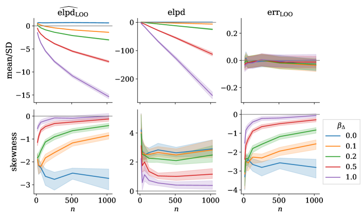
Figure 12: Illustration of the estimated mean relative to the standard deviation and skewness for ${\widehat{\mathrm{elpd}}_{\mathrm{\scriptscriptstyle LOO}}\bigr{(}{\mathrm{M}_{a},\mathrm{M}_{b}}\mid y\bigl{)}}$, ${\mathrm{elpd}\bigr{(}{\mathrm{M}_{a},\mathrm{M}_{b}}\mid y\bigl{)}}$, and for the error ${\mathrm{err}_{\mathrm{\scriptscriptstyle LOO}}\bigr{(}{\mathrm{M}_{a},\mathrm{M}_{b}}\mid y\bigl{)}}$ as a function of the data size $n$ for various non-shared covariate effects $\beta_{\Delta}$. The solid lines corresponds to the median and the shaded area to the 95 % confidence interval from Bayesian bootstrap (BB) sample of size 2000 using the weighted moment estimators presented by Rimoldini (2014). As the effect of $\beta_{\Delta}$ is symmetric, the problem is simulated only with positive $\beta_{\Delta}$.Similar behaviour can be observed in Figure 4 for analogous experiment conditional for the design matrix $X$ and model variance $\tau^{2}$. In this case, however, while not greatly affecting the skewness of the error ${\mathrm{err}_{\mathrm{\scriptscriptstyle LOO}}\bigr{(}{\mathrm{M}_{a},\mathrm{M}_{b}}\mid y\bigl{)}}$, the skewness of the ${\mathrm{elpd}\bigr{(}{\mathrm{M}_{a},\mathrm{M}_{b}}\mid y\bigl{)}}$ decreases, when $\beta_{\Delta}$ grows.

Figure 12 illustrates the relative mean and skewness for the sampling distribution ${\widehat{\mathrm{elpd}}_{\mathrm{\scriptscriptstyle LOO}}\bigr{(}{\mathrm{M}_{a},\mathrm{M}_{b}}\mid y\bigl{)}}$, for the distribution of the estimand ${\mathrm{elpd}\bigr{(}{\mathrm{M}_{a},\mathrm{M}_{b}}\mid y\bigl{)}}$, and for the error distribution ${\mathrm{err}_{\mathrm{\scriptscriptstyle LOO}}\bigr{(}{\mathrm{M}_{a},\mathrm{M}_{b}}\mid y\bigl{)}}$ estimated from the simulated experiments as a function of the data size $n$ for different non-shared covariates’ effects $\beta_{\Delta}$.These results indicate, that the moments behave quite similarly as in the analysis conditional on the design matrix $X$ and model variance $\tau$ in Section 3. Similar to the situation with conditionalised design matrix $X$ and model variance $\tau$, it can be seen from the figure that the when the non-shared covariate effect $\beta_{\Delta}$ grows, the difference in the predictive performance grows and the LOO-CV method becomes more likely to pick the correct model. Similar behaviour can be observed, when the data size $n$ grows and $|\beta_{\Delta}|>0$. However, when $\beta_{\Delta}=0$, the difference in the predictive performance stays zero and the LOO-CV method is slightly more likely to pick the simpler model regardless of $n$. The relative mean of the error confirms that the bias of the LOO-CV estimator is relatively small with all applied $n$ and $\beta_{\Delta}$.

By analysing the estimated skewness in Figure 12, it can be seen that the absolute skewness of ${\widehat{\mathrm{elpd}}_{\mathrm{\scriptscriptstyle LOO}}\bigr{(}{\mathrm{M}_{a},\mathrm{M}_{b}}\mid y\bigl{)}}$ and ${\mathrm{err}_{\mathrm{\scriptscriptstyle LOO}}\bigr{(}{\mathrm{M}_{a},\mathrm{M}_{b}}\mid y\bigl{)}}$ is bigger when $\beta_{\Delta}$ is closer to zero and the models are more similar in predictive performance. While in the case of conditionalised design matrix $X$ and model variance $\tau$ in Section 3, the skewness of ${\mathrm{elpd}\bigr{(}{\mathrm{M}_{a},\mathrm{M}_{b}}\mid y\bigl{)}}$ is similar with all $\beta_{\Delta}$, in the simulated experiment this skewness decreases when $\beta_{\Delta}$ grows. When $|\beta_{\Delta}|>0$, the absolute skewness of ${\widehat{\mathrm{elpd}}_{\mathrm{\scriptscriptstyle LOO}}\bigr{(}{\mathrm{M}_{a},\mathrm{M}_{b}}\mid y\bigl{)}}$ and ${\mathrm{err}_{\mathrm{\scriptscriptstyle LOO}}\bigr{(}{\mathrm{M}_{a},\mathrm{M}_{b}}\mid y\bigl{)}}$ decreases towards zero when $n$ grows. Otherwise, when $\beta_{\Delta}=0$, similar to the problem setting in the analytic case study in Section 3, the skewness does not fade off when $n$ grows. These results show that the problematic skewness can occur when the models are close in predictive performance and with smaller sample sizes.

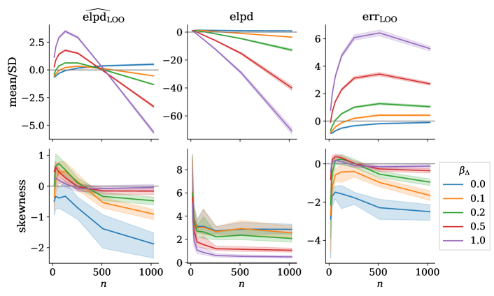
Figure 13: Illustration of the estimated mean relative to the standard deviation and skewness for ${\widehat{\mathrm{elpd}}_{\mathrm{\scriptscriptstyle LOO}}\bigr{(}{\mathrm{M}_{a},\mathrm{M}_{b}}\mid y\bigl{)}}$, ${\mathrm{elpd}\bigr{(}{\mathrm{M}_{a},\mathrm{M}_{b}}\mid y\bigl{)}}$, and for the error ${\mathrm{err}_{\mathrm{\scriptscriptstyle LOO}}\bigr{(}{\mathrm{M}_{a},\mathrm{M}_{b}}\mid y\bigl{)}}$ as a function of the data size $n$ for various non-shared covariate effects $\beta_{\Delta}$, when there are an outlier observation in the data. The solid lines corresponds to the median and the shaded area to the 95 % confidence interval from Bayesian bootstrap (BB) sample of size 2000 using the weighted moment estimators presented by Rimoldini (2014). As the effect of $\beta_{\Delta}$ is symmetric, the problem is simulated only with positive $\beta_{\Delta}$.

Figure 13 illustrates the relative mean and skewness for the sampling distribution ${\widehat{\mathrm{elpd}}_{\mathrm{\scriptscriptstyle LOO}}\bigr{(}{\mathrm{M}_{a},\mathrm{M}_{b}}\mid y\bigl{)}}$, for the distribution of the estimand ${\mathrm{elpd}\bigr{(}{\mathrm{M}_{a},\mathrm{M}_{b}}\mid y\bigl{)}}$, and for the error distribution ${\mathrm{err}_{\mathrm{\scriptscriptstyle LOO}}\bigr{(}{\mathrm{M}_{a},\mathrm{M}_{b}}\mid y\bigl{)}}$ estimated from the simulated experiments as a function of the data size $n$ for different non-shared covariates’ effects $\beta_{\Delta}$ when there is an outlier observation in the data. Compared to the analogous plot without the outlier in Figure 12, introducing the outlier affects the distribution of ${\widehat{\mathrm{elpd}}_{\mathrm{\scriptscriptstyle LOO}}\bigr{(}{\mathrm{M}_{a},\mathrm{M}_{b}}\mid y\bigl{)}}$ more than of the distribution of ${\mathrm{elpd}\bigr{(}{\mathrm{M}_{a},\mathrm{M}_{b}}\mid y\bigl{)}}$. This is plausible considering the leave-one-out technique used in the estimator. Due to the difference in the distribution of ${\widehat{\mathrm{elpd}}_{\mathrm{\scriptscriptstyle LOO}}\bigr{(}{\mathrm{M}_{a},\mathrm{M}_{b}}\mid y\bigl{)}}$, the error ${\mathrm{err}_{\mathrm{\scriptscriptstyle LOO}}\bigr{(}{\mathrm{M}_{a},\mathrm{M}_{b}}\mid y\bigl{)}}$ is also affected. The effect is greater when the non-shared covariates effect $\beta_{\Delta}$ is bigger.

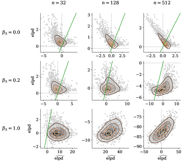
Figure 14: Illustration of joint distribution of ${\widehat{\mathrm{elpd}}_{\mathrm{\scriptscriptstyle LOO}}\bigr{(}{\mathrm{M}_{a},\mathrm{M}_{b}}\mid y\bigl{)}}$ and ${\mathrm{elpd}\bigr{(}{\mathrm{M}_{a},\mathrm{M}_{b}}\mid y\bigl{)}}$ for various data sizes $n$, non-shared covariate effects $\beta_{\Delta}$, and an outlier in the data. The outlier scaling coefficient is set to $\mu_{\star\mathrm{r}}=20$. Green diagonal line indicates where ${\widehat{\mathrm{elpd}}_{\mathrm{\scriptscriptstyle LOO}}\bigr{(}{\mathrm{M}_{a},\mathrm{M}_{b}}\mid y\bigl{)}}={\mathrm{elpd}\bigr{(}{\mathrm{M}_{a},\mathrm{M}_{b}}\mid y\bigl{)}}$.

Figure 14 illustrates the joint distribution of the estimator ${\widehat{\mathrm{elpd}}_{\mathrm{\scriptscriptstyle LOO}}\bigr{(}{\mathrm{M}_{a},\mathrm{M}_{b}}\mid y\bigl{)}}$ and the estimand ${\mathrm{elpd}\bigr{(}{\mathrm{M}_{a},\mathrm{M}_{b}}\mid y\bigl{)}}$ when there is an outlier observation present. Similar to the case without an outlier illustrated in Figure 6, although in a slightly lesser degree, the estimator and the estimand get negatively correlated when the models’ predictive performances get more similar. In the outlier-case, however, the estimator is clearly biased and using the LOO-CV method is problematic. For example, in the case where $n=128$ and $\beta_{\Delta}=1.0$, the distributions of ${\widehat{\mathrm{elpd}}_{\mathrm{\scriptscriptstyle LOO}}\bigr{(}{\mathrm{M}_{a},\mathrm{M}_{b}}\mid y\bigl{)}}$ and ${\mathrm{elpd}\bigr{(}{\mathrm{M}_{a},\mathrm{M}_{b}}\mid y\bigl{)}}$ lies in the opposite sides of sign and LOO-CV method will almost surely pick the wrong model.

Figure 15 illustrates the behaviour of the error relative to the standard deviation ${\mathrm{err}_{\mathrm{\scriptscriptstyle LOO}}\bigr{(}{\mathrm{M}_{a},\mathrm{M}_{b}}\mid y\bigl{)}}\big{/}\allowbreak\operatorname{SD}\bigl{(}{\mathrm{elpd}\bigr{(}{\mathrm{M}_{a},\mathrm{M}_{b}}\mid y\bigl{)}}\bigr{)}$ for various non-shared covariate effects $\beta_{\Delta}$ and data sizes $n$ with and without an outlier observation. It can be seen from the figure that without outliers, the mean of the relative error is near zero in all settings, so the bias in the LOO-CV estimator is small. When there is an outlier present in the data (Scenario 2), the relative error’s mean usually clearly deviates from zero, and the estimator is biased. Whether LOO-CV estimates the difference in the predictive performance to be further away or closer to zero or of a different sign depends on the situation. Figure 16 illustrates the behaviour of

$$\operatorname{sign}\Bigl{(}{\mathrm{elpd}\bigr{(}{\mathrm{M}_{a},\mathrm{M}_{b}}\mid y\bigl{)}}\Bigr{)}\frac{{\mathrm{err}_{\mathrm{\scriptscriptstyle LOO}}\bigr{(}{\mathrm{M}_{a},\mathrm{M}_{b}}\mid y\bigl{)}}}{\operatorname{SD}\Bigl{(}{\mathrm{elpd}\bigr{(}{\mathrm{M}_{a},\mathrm{M}_{b}}\mid y\bigl{)}}\Bigr{)}}\,,$$

the relative error directed towards ${\mathrm{elpd}\bigr{(}{\mathrm{M}_{a},\mathrm{M}_{b}}\mid y\bigl{)}}=0$, for various non-shared covariate effects $\beta_{\Delta}$ and data sizes $n$ with and without an outlier observation. It can be seen from the figure, that with an outlier observation, LOO-CV often estimates the difference in the predictive performance to be smaller or of the opposite sign than the estimand ${\mathrm{elpd}\bigr{(}{\mathrm{M}_{a},\mathrm{M}_{b}}\mid y\bigl{)}}$.

Figure 15: Distribution of the relative error ${\mathrm{err}_{\mathrm{\scriptscriptstyle LOO}}\bigr{(}{\mathrm{M}_{a},\mathrm{M}_{b}}\mid y\bigl{)}}\big{/}\operatorname{SD}\mathopen{}\mathclose{{}\left({\mathrm{elpd}\bigr{(}{\mathrm{M}_{a},\mathrm{M}_{b}}\mid y\bigl{)}}}\right)$ for different data sizes $n$ and non-shared covariate effects $\beta_{\Delta}$. In the left column, there are no outliers in the data, and in the right column, there is one extreme outlier with deviated mean of 20 times the standard deviation of $y_{i}$. The distributions are visualised using letter-value plots or boxenplots (Hofmann et al., 2017). The black lines correspond to the median of the distribution, and yellow lines indicate the mean. With an extreme outlier in the data (Scenario 2), the bias can be considerable. Whether LOO-CV estimates the difference in the predictive performance to be further away or closer to zero or of different sign, depends on the situation.

Figure 16: Distribution of $\operatorname{sign}\mathopen{}\mathclose{{}\left({}^{\mathrm{sv}}{\mathrm{elpd}}}\right){}^{\mathrm{sv}}{\mathrm{err}_{\mathrm{\scriptscriptstyle LOO}}}\big{/}\operatorname{SD}\mathopen{}\mathclose{{}\left({}^{\mathrm{sv}}{\mathrm{elpd}}}\right)$, the relative error directed towards ${}^{\mathrm{sv}}{\mathrm{elpd}}=0$, in a model comparison setting (omitting arguments $({\mathrm{M}_{a},\mathrm{M}_{b}}\mid y)$ for clarity) for different data sizes $n$ and non-shared covariate effects $\beta_{\Delta}$. Negative values indicate that LOO-CV estimates the difference in the predictive performance being smaller or of the opposite sign and positive values indicate the difference is larger. In the left column, there is no outliers in the data, and in the right column, there is one outlier with deviated mean of 20 times the standard deviation of $y_{i}$. The distributions are visualised using letter-value plots or boxenplots (Hofmann et al., 2017). The black lines correspond to the median of the distribution and yellow lines indicate the mean. With an outlier observation, the directed relative error is typically negative.

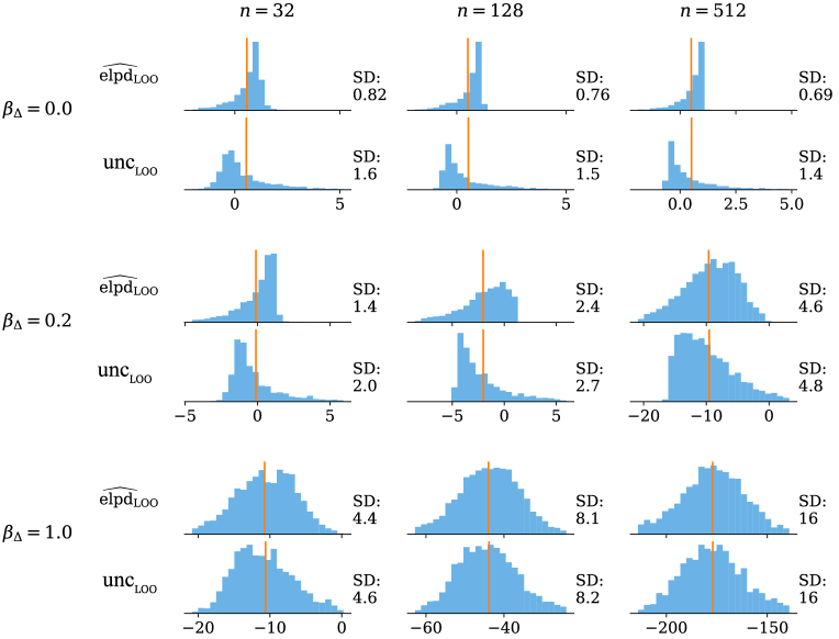
Figure 17: Illustration of the distributions of ${\widehat{\mathrm{elpd}}_{\mathrm{\scriptscriptstyle LOO}}\bigr{(}{\mathrm{M}_{a},\mathrm{M}_{b}}\mid y\bigl{)}}$ and ${\mathrm{unc}_{\mathrm{\scriptscriptstyle LOO}}\bigr{(}{\mathrm{M}_{a},\mathrm{M}_{b}}\mid y\bigl{)}}$, where $y$ is such that ${\widehat{\mathrm{elpd}}_{\mathrm{\scriptscriptstyle LOO}}\bigr{(}{\mathrm{M}_{a},\mathrm{M}_{b}}\mid y\bigl{)}}=\operatorname{E}\mathopen{}\mathclose{{}\left[{\widehat{\mathrm{elpd}}_{\mathrm{\scriptscriptstyle LOO}}\bigr{(}{\mathrm{M}_{a},\mathrm{M}_{b}}\mid y\bigl{)}}}\right]$, for various data sizes $n$ and non-shared covariate effects $\beta_{\Delta}$. The yellow lines show the means of the distributions and the corresponding sample standard deviation is displayed next to each histogram. In the problematic cases with small $n$ and $\beta_{\Delta}$, there is a weak connection in the skewness of the sampling and the error distributions. Thus, even with better estimator for the sampling distribution, the estimation of the uncertainty is badly calibrated. For brevity, model labels are omitted in the notation in the figure.

Figure 17 illustrates the difference between the sampling distribution ${\widehat{\mathrm{elpd}}_{\mathrm{\scriptscriptstyle LOO}}\bigr{(}{\mathrm{M}_{a},\mathrm{M}_{b}}\mid y\bigl{)}}$ and the uncertainty distribution

$${\mathrm{unc}_{\mathrm{\scriptscriptstyle LOO}}\bigr{(}{\mathrm{M}_{a},\mathrm{M}_{b}}\mid y\bigl{)}}={\widehat{\mathrm{elpd}}_{\mathrm{\scriptscriptstyle LOO}}\bigr{(}{\mathrm{M}_{a},\mathrm{M}_{b}}\mid y\bigl{)}}-{\mathrm{err}_{\mathrm{\scriptscriptstyle LOO}}\bigr{(}{\mathrm{M}_{a},\mathrm{M}_{b}}\mid y\bigl{)}}\,.$$ (411)

Here $y$ is selected such that ${\widehat{\mathrm{elpd}}_{\mathrm{\scriptscriptstyle LOO}}\bigr{(}{\mathrm{M}_{a},\mathrm{M}_{b}}\mid y\bigl{)}}=\operatorname{E}\mathopen{}\mathclose{{}\left[{\widehat{\mathrm{elpd}}_{\mathrm{\scriptscriptstyle LOO}}\bigr{(}{\mathrm{M}_{a},\mathrm{M}_{b}}\mid y\bigl{)}}}\right]$ so that, in addition to the shape, the location of the former distribution can be directly compared to the location of the latter one. It can be seen from the figure, that the distributions match when one model is clearly better than the other. When the models are more similar in predictive performance, however, the distribution of ${\widehat{\mathrm{elpd}}_{\mathrm{\scriptscriptstyle LOO}}\bigr{(}{\mathrm{M}_{a},\mathrm{M}_{b}}\mid y\bigl{)}}$ has smaller variability than in the distribution of the uncertainty ${\mathrm{unc}_{\mathrm{\scriptscriptstyle LOO}}\bigr{(}{\mathrm{M}_{a},\mathrm{M}_{b}}\mid y\bigl{)}}$ and the distribution is skewed to the wrong direction. Nevertheless, as the bias of the approximation is small, the means of the distributions are close in all problem settings.

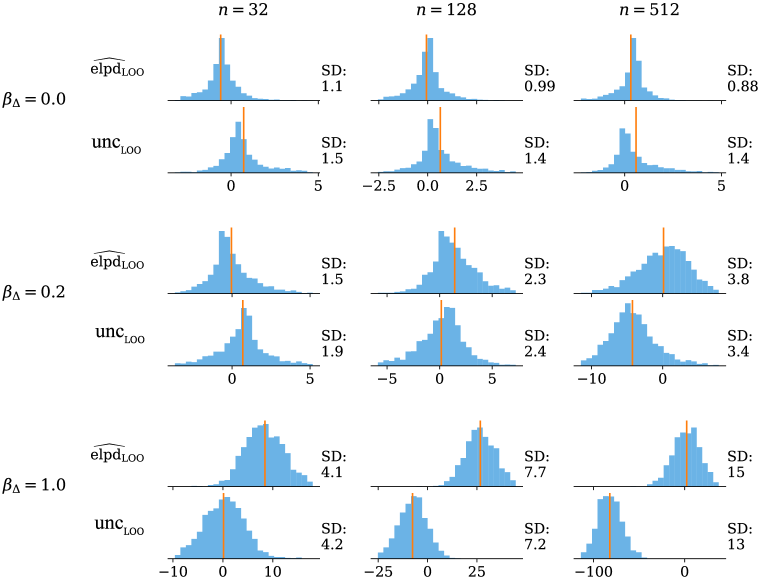
Figure 18: Illustration of the distributions of ${\widehat{\mathrm{elpd}}_{\mathrm{\scriptscriptstyle LOO}}\bigr{(}{\mathrm{M}_{a},\mathrm{M}_{b}}\mid y\bigl{)}}$ and ${\mathrm{unc}_{\mathrm{\scriptscriptstyle LOO}}\bigr{(}{\mathrm{M}_{a},\mathrm{M}_{b}}\mid y\bigl{)}}$, where $y$ is such that ${\widehat{\mathrm{elpd}}_{\mathrm{\scriptscriptstyle LOO}}\bigr{(}{\mathrm{M}_{a},\mathrm{M}_{b}}\mid y\bigl{)}}=\operatorname{E}\mathopen{}\mathclose{{}\left[{\widehat{\mathrm{elpd}}_{\mathrm{\scriptscriptstyle LOO}}\bigr{(}{\mathrm{M}_{a},\mathrm{M}_{b}}\mid y\bigl{)}}}\right]$, for various data sizes $n$, non-shared covariate effects $\beta_{\Delta}$, and an outlier in the data. The yellow lines show the means of the distributions and the corresponding sample standard deviation is displayed next to each histogram. For brevity, model labels are omitted in the notatin in the figure.

Figure 18 illustrates the difference of the sampling distribution ${\widehat{\mathrm{elpd}}_{\mathrm{\scriptscriptstyle LOO}}\bigr{(}{\mathrm{M}_{a},\mathrm{M}_{b}}\mid y\bigl{)}}$ and the uncertainty distribution ${\mathrm{unc}_{\mathrm{\scriptscriptstyle LOO}}\bigr{(}{\mathrm{M}_{a},\mathrm{M}_{b}}\mid y\bigl{)}}$ when there is an outlier observation present. Compared to the non-outlier case shown in Figure 17, in this model misspecification setting, the distributions are not notably skewed to the opposite directions anymore but, as the approximations are significantly biased, the means are clearly different.

Figure 19 illustrates the problem of underestimation of the variance with small data sizes $n$ (Scenario 3) and models with more similar predictive performances (Scenario 1).

Figure 19: Distribution of the ratio ${\widehat{\mathrm{SE}}_{\mathrm{\scriptscriptstyle LOO}}\bigr{(}{\mathrm{M}_{a},\mathrm{M}_{b}}\mid y\bigl{)}}\,\Big{/}\,\operatorname{SE}\Bigl{(}{\mathrm{err}_{\mathrm{\scriptscriptstyle LOO}}\bigr{(}{\mathrm{M}_{a},\mathrm{M}_{b}}\mid y\bigl{)}}\Bigr{)}$ for different data sizes $n$ and non-shared covariate effects $\beta_{\Delta}$. The red line highlights the target ration of 1. The distributions are visualised using letter-value plots or boxenplots (Hofmann et al., 2017). The black lines correspond to the median of the distribution. The variability is predominantly underestimated, with small $\beta_{\Delta}$ (Scenario 1) and small $n$ (Scenario 3).

Figure 20: Distribution of the ratio ${\widehat{\mathrm{SE}}_{\mathrm{\scriptscriptstyle LOO}}\bigr{(}{\mathrm{M}_{a},\mathrm{M}_{b}}\mid y\bigl{)}}\,\Big{/}\,\operatorname{SE}\Bigl{(}{\mathrm{err}_{\mathrm{\scriptscriptstyle LOO}}\bigr{(}{\mathrm{M}_{a},\mathrm{M}_{b}}\mid y\bigl{)}}\Bigr{)}$ for different data sizes $n$ and non-shared covariate effects $\beta_{\Delta}$, when there is an outlier observation in the data. The red line highlights the target ration of 1. The distributions are visualised using letter-value plots or boxenplots (Hofmann et al., 2017). The black lines corresponds to the median of the distribution.

Figure 20 illustrates the problem of underestimation of the variance with small data sizes $n$ and models with more similar predictive performances, when there is an outlier observation in the data. Compared to the non-outlier case shown in Figure 19, in this model misspecification setting, the ratio is situationally also significantly larger than one so that the uncertainty is overestimated. In these situations, as demonstrated for example in Figure 14 the estimator is biased so that the overestimation is understandable and acceptable.

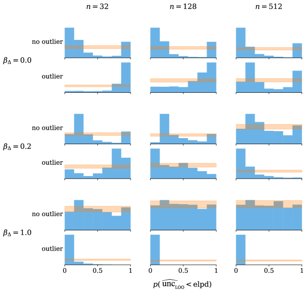
Figure 21: Calibration of the theoretical approximation based on ${\widehat{\mathrm{elpd}}_{\mathrm{\scriptscriptstyle LOO}}\bigr{(}{\mathrm{M}_{a},\mathrm{M}_{b}}\mid y\bigl{)}}$ centred around ${\widehat{\mathrm{elpd}}_{\mathrm{\scriptscriptstyle LOO}}\bigr{(}{\mathrm{M}_{a},\mathrm{M}_{b}}\mid y\bigl{)}}$ for various data sizes $n$ and non-shared covariate effects $\beta_{\Delta}$, when there is an outlier observation in the data. The histograms show the distribution of $p\Bigl{(}{\widehat{\mathrm{unc}}_{\mathrm{\scriptscriptstyle LOO}}\bigr{(}{\mathrm{M}_{a},\mathrm{M}_{b}}\mid y\bigl{)}}<{\mathrm{elpd}\bigr{(}{\mathrm{M}_{a},\mathrm{M}_{b}}\mid y\bigl{)}}\Bigr{)}$, which would be uniform in a case of optimal calibration.

Figure 21 illustrates the calibration of the theoretical estimate based on the true distribution of ${\widehat{\mathrm{elpd}}_{\mathrm{\scriptscriptstyle LOO}}\bigr{(}{\mathrm{M}_{a},\mathrm{M}_{b}}\mid y\bigl{)}}$ centred around ${\widehat{\mathrm{elpd}}_{\mathrm{\scriptscriptstyle LOO}}\bigr{(}{\mathrm{M}_{a},\mathrm{M}_{b}}\mid y\bigl{)}}$ in various problem settings, when there is an outlier observation in the data. It can be seen that the sampling distribution provides a good calibration only in the case of no outlier and large $\beta_{\Delta}$ or, to some degree, large $n$.

Figures 22 and 23 provide additional information related to the experiments discussed in Section 4.5. Figure 22 shows the relative error ${\mathrm{err}_{\mathrm{\scriptscriptstyle LOO}}\bigr{(}{\mathrm{M}_{a},\mathrm{M}_{b}}\mid y\bigl{)}}\big{/}\operatorname{SD}\mathopen{}\mathclose{{}\left({\mathrm{elpd}\bigr{(}{\mathrm{M}_{a},\mathrm{M}_{b}}\mid y\bigl{)}}}\right)$ for different data sizes, the non-shared coefficient is equal to 0.5, and without outlier observations. The relative errors are symmetrical, and mean and median close to zero; confirming that also in the extended examples, the bias goes asymptotically to zero (Section 3 of this paper;Arlot and Celisse, 2010, Section 5.1; Watanabe, 2010).

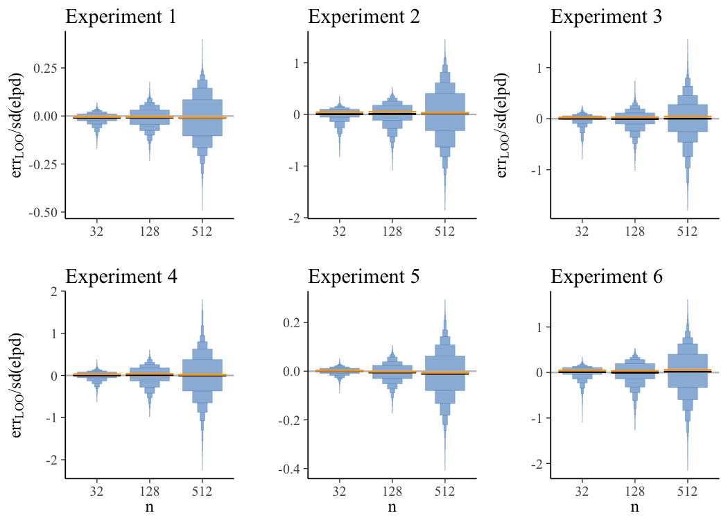
Figure 22: Distribution of the relative error for different data sizes $n=32,128,512$ and for the non-shared covariate effect 0.5. The distributions are visualised using letter-value plots or boxenplots, the black lines correspond to the median of the distribution, yellow lines indicate the mean, and the x-axis indicate the different data sizes n

Figure 23 compares the normal uncertainty approximation for data size $n=128$, with a non-shared covariate effect $\beta_{\Delta}=0.5$. The results show that when models differ in their predictive performance slightly, the normal approximation provides a good fit for the LOO-CV uncertainty even in problematic scenarios where the number of observations is relatively small (Scenario 3).

Figure 23: Approximated uncertainty using a normal distribution. The histogram represents the calculated uncertainty defined in equation (8) shifted by its mean, the orange line represents the normal approximation defined in Section 2.2, and the vertical line corresponds to the ${\mathrm{elpd}\bigr{(}{\mathrm{M}_{a},\mathrm{M}_{b}}\mid y\bigl{)}}$

Appendix F Study case: Analysing Radon data set

Radon is a radioactive gas that enters homes through contact points with the ground. It is a carcinogen that is the primary cause of lung cancer in non-smokers. Radon levels vary significantly from household to household. The EPA studied radon levels in 80,000 houses, of which $n=12,777$ records are available. A significant predictor is a measurement in the basement or first floor (radon higher in basements), and the hierarchy in this study is households within the county. The two proposed models are:

• $M_{a}:\mathrm{logRadon}=\beta_{0}+\beta_{1}\mathrm{floor}+\varepsilon,$

• $M_{b}:\mathrm{logRadon}_{j}=\beta_{0}+\beta_{1}\mathrm{floor}+\alpha_{j}+\varepsilon,$ and $\alpha_{j}\sim n(\alpha_{0},\sigma_{\alpha}),\text{ for }j=1,2,\ldots,k.$

Where $\varepsilon$ is a random variable normally distributed with unknown variance ($\varepsilon\sim n(0,\sigma)$), $\beta_{0},\beta_{1}\in\mathbb{R}$ are unknown parameters with weak prior distributions, floor is the covariate that represents the measurement in the basement or first floor, $\alpha_{j}\in\mathbb{R}$ are the group effects for the $k=386$ counties, $\alpha_{0}\in\mathbb{R}$ and $\sigma_{\alpha}>0$ are the location and scale parameters for the group effects respectively. The experiment consists on evaluating the performance of ${\widehat{\mathrm{elpd}}_{\mathrm{\scriptscriptstyle LOO}}\bigr{(}{\mathrm{M}_{a},\mathrm{M}_{b}}\mid\mathrm{Radon}\bigl{)}}$, and ${\widehat{\mathrm{SE}}_{\mathrm{\scriptscriptstyle LOO}}\bigr{(}{\mathrm{M}_{a},\mathrm{M}_{b}}\mid\mathrm{Radon}\bigl{)}}$ for estimating the real ${\mathrm{elpd}\bigr{(}{\mathrm{M}_{a},\mathrm{M}_{b}}\mid\mathrm{Radon}\bigl{)}}$.

Estimating the elpd

First, split the data set into two equal parts (train and test sets), randomly selecting the observations for the train set using a random stratified sampling, where the groups represent the different counties. Second, fit the two models using the train set, estimate the ${\widehat{\mathrm{elpd}}_{\mathrm{\scriptscriptstyle LOO}}\bigr{(}{\mathrm{M}_{a},\mathrm{M}_{b}}\mid\mathrm{Train}\bigl{)}}$ and ${\widehat{\mathrm{SE}}_{\mathrm{\scriptscriptstyle LOO}}\bigr{(}{\mathrm{M}_{a},\mathrm{M}_{b}}\mid\mathrm{Train}\bigl{)}}$ values. Finally, calculate the ${\mathrm{elpd}\bigr{(}{\mathrm{M}_{a},\mathrm{M}_{b}}\mid Test\bigl{)}}$ estimate utilising the test set.

The estimated LOO value is ${\widehat{\mathrm{elpd}}_{\mathrm{\scriptscriptstyle LOO}}\bigr{(}{\mathrm{M}_{a},\mathrm{M}_{b}}\mid\mathrm{Train}\bigl{)}}=-749.3$ and standard error ${\widehat{\mathrm{SE}}_{\mathrm{\scriptscriptstyle LOO}}\bigr{(}{\mathrm{M}_{a},\mathrm{M}_{b}}\mid\mathrm{Train}\bigl{)}}=38.5$. For the test set, the calculated is

$${\mathrm{elpd}\bigr{(}{\mathrm{M}_{a},\mathrm{M}_{b}}\mid Test\bigl{)}}=-731.7.$$

Both estimator and elpd favour the Hierarchical (${\mathrm{M}_{b}}$) over the linear model (${\mathrm{M}_{a}}$), and due to the big sample size and the difference in prediction in both models, we are certain in select model ${\mathrm{M}_{b}}$. Although the LOO estimator and the elpd are not so different for this data set, the estimated uncertainty is helpful for a proper evaluation of the performance of LOO.

Evaluating the uncertainty of the LOO estimator

In this experiment, we use a Bootstrap re-sample procedure for evaluating the uncertainty of the LOO estimator. For this experiment we obtain $500$ bootstrap replicates, and the process for each iteration is as follow:

1. Generate a bootstrap sample $B_{l},$ $l=1,2,\ldots,500$ using a random stratified sample, where the counties represent the groups.

2. Fit both models and calculate the ${\widehat{\mathrm{elpd}}_{\mathrm{\scriptscriptstyle LOO}}\bigr{(}{\mathrm{M}_{a},\mathrm{M}_{b}}\mid B_{l}\bigl{)}}$, and ${\widehat{\mathrm{SE}}_{\mathrm{\scriptscriptstyle LOO}}\bigr{(}{\mathrm{M}_{a},\mathrm{M}_{b}}\mid B_{l}\bigl{)}}$.

3. Extract a random sample using the remaining data $B_{l}^{{}^{\prime}}\subseteq B_{l}^{c}$ and calculate the real ${\mathrm{elpd}\bigr{(}{\mathrm{M}_{a},\mathrm{M}_{b}}\mid B_{l}^{{}^{\prime}}\bigl{)}}$.

   Notice that $\{B_{l}^{{}^{\prime}}\}_{l=1}^{500}$ is also a Bootstrap sample, where every $B_{l}^{{}^{\prime}}$ is an independent sample of $B_{l}$.

4. Obtain a Bootstrap sample for the error using Equation (8)

   $${\mathrm{err}_{\mathrm{\scriptscriptstyle LOO}}\bigr{(}{\mathrm{M}_{a},\mathrm{M}_{b}}\mid B_{l}\bigl{)}}={\widehat{\mathrm{elpd}}_{\mathrm{\scriptscriptstyle LOO}}\bigr{(}{\mathrm{M}_{a},\mathrm{M}_{b}}\mid B_{l}\bigl{)}}-{\mathrm{elpd}\bigr{(}{\mathrm{M}_{a},\mathrm{M}_{b}}\mid B_{l}^{{}^{\prime}}\bigl{)}}.$$

5. A sample for the uncertainty is

   $${\mathrm{elpd}\bigr{(}{\mathrm{M}_{a},\mathrm{M}_{b}}\mid B_{l}\bigl{)}}={\widehat{\mathrm{elpd}}_{\mathrm{\scriptscriptstyle LOO}}\bigr{(}{\mathrm{M}_{a},\mathrm{M}_{b}}\mid\mathrm{Train}\bigl{)}}+{\mathrm{err}_{\mathrm{\scriptscriptstyle LOO}}\bigr{(}{\mathrm{M}_{a},\mathrm{M}_{b}}\mid B_{l}\bigl{)}},$$

where ${\widehat{\mathrm{elpd}}_{\mathrm{\scriptscriptstyle LOO}}\bigr{(}{\mathrm{M}_{a},\mathrm{M}_{b}}\mid\mathrm{Train}\bigl{)}}$ represents the LOO estimate using the original train set, and $\{{\mathrm{elpd}\bigr{(}{\mathrm{M}_{a},\mathrm{M}_{b}}\mid B_{l}\bigl{)}}\}_{l=1}^{500}$ represents the obtained bootstrap sample for the uncertainty. The primary purpose of this procedure is to obtain a well-calibrated sample of the LOO estimators uncertainty that validates our previous LOO estimates for model selection in the Radon data analysis.

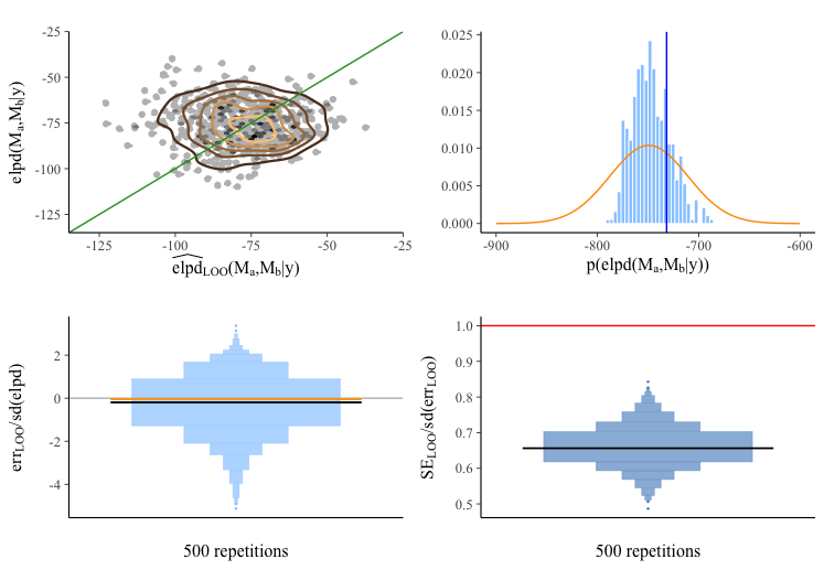
Figure 24: The top-left plot illustrates the joint distribution of elpd and its estimator. The top right plot demonstrates the normal approximation of the uncertainty of the LOO estimator for approximating the elpd, the light blue bars represent the distribution of the uncertainty calculated using equation (10), the vertical blue line represents the elpd calculated using the test set, and the orange line represents the normal approximation for the uncertainty using estimate and SE of the train set. The bottom-left plot shows the distribution of the relative errors. The bottom-right plot illustrates the distribution of the ratio LOO estandar error. The red line highlights the target ratio of 1. The distributions are visualised using boxenplots, and the black lines correspond to the median of the distribution.

The top-right plot in Figure 24 does not show a negative correlation or bias, indicating that the LOO estimate explains the $elpd$. The top-left plot shows that the uncertainty and its approximation captures the $elpd$ calculated with the test set, indicating a good calibration of the uncertainty for the Radon data set. Notice the difference in scales between the top-left and top-right plots is due to the used sample size in every bootstrap approximation being smaller than the sample size in the train set, therefore the estimates ${\widehat{\mathrm{elpd}}_{\mathrm{\scriptscriptstyle LOO}}\bigr{(}{\mathrm{M}_{a},\mathrm{M}_{b}}\mid B_{l}\bigl{)}}$ and ${\widehat{\mathrm{elpd}}_{\mathrm{\scriptscriptstyle LOO}}\bigr{(}{\mathrm{M}_{a},\mathrm{M}_{b}}\mid B_{l}\bigl{)}}$ are different in magnitude from ${\widehat{\mathrm{elpd}}_{\mathrm{\scriptscriptstyle LOO}}\bigr{(}{\mathrm{M}_{a},\mathrm{M}_{b}}\mid train\bigl{)}}$ and ${\mathrm{unc}_{\mathrm{\scriptscriptstyle LOO}}\bigr{(}{\mathrm{M}_{a},\mathrm{M}_{b}}\mid B_{l}\bigl{)}}$. The standard errors in the top-left plot are symmetric and located at zero, validating the possible good calibration of the uncertainty observed at the top-right plot. Finally, in the bottom-right plot, the ratio is not centred at one, which shows that our bootstrap estimate of the $SE_{LOO}$ underestimates the actual dispersion for the uncertainty of the LOO estimator.