Edge-Induced Excitations in Bi₂Te₃ from Spatially-Resolved Electron Energy-Gain Spectroscopy

Abstract

Among the many potential applications of topological insulator materials, their broad potential for the development of novel tunable plasmonics at THz and mid-infrared frequencies for quantum computing, terahertz detectors, and spintronic devices is particularly attractive. The required understanding of the intricate relationship between nanoscale crystal structure and the properties of the resulting plasmonic resonances remains, however, elusive for these materials. Specifically, edge- and surface-induced plasmonic resonances, and other collective excitations, are often buried beneath the continuum of electronic transitions, making it difficult to isolate and interpret these signals using techniques such as electron energy-loss spectroscopy (EELS). Here we focus on the experimentally clean energy-gain EELS region to characterise collective excitations in the topologically insulating material Bi₂Te₃ and correlate them with the underlying crystalline structure with nanoscale resolution. We identify with high significance the presence of a distinct energy-gain peak around $-0.8$ eV, with spatially-resolved maps revealing that its intensity is markedly enhanced at the edge regions of the specimen. Our findings illustrate the reach of energy-gain EELS analyses to accurately map collective excitations in quantum materials, a key asset in the quest towards new tunable plasmonic devices.

Introduction

Topological insulator (TI) materials, such as $\text{Bi}_{2}\text{Te}_{3}$ [1, 2, 3] and Bi₂Se₃, possess unique properties that make them well suited for the design of nanoplasmonic devices operating in the THz and mid-infrared frequency ranges. [4, 5, 6, 7, 8] Topological insulators can also support plasmonic excitations, collective oscillations of electrons that interact strongly with light or other electrons and lead to enhanced light-matter interactions such as strong scattering, absorption, and emission. In particular, low-energy plasmons [9] have been reported in $\text{Bi}_{2}\text{Te}_{3}$ below $3$ eV while correlated plasmons at energies $\sim 1$ eV have been identified for Bi₂Se₃ [10]. In this context, advancing our understanding of how to optimally deploy TIs for the development of tunable plasmonic devices that operate efficiently in optical frequencies has the potential to benefit a wide range of applications, including quantum computing [11, 12], terahertz detectors [13], and spintronic devices [14].

In recent years, significant progress has been achieved in resolving plasmon resonances at the nanoscale, providing valuable information about the spatial and spectral distribution of plasmonic modes. To this end, electron-based spectroscopic techniques such as electron energy-loss spectroscopy (EELS) have demonstrated their suitability to investigate the electronic and optical properties of a wide range of materials, including the study of their plasmonic resonances. [15, 16, 17, 18, 19, 20, 21] In parallel, advances in transmission electron microscopy (TEM) have resulted in novel opportunities for scrutinizing the functionalities of nanostructured materials. For instance, the incorporation of monochromators and aberration correctors makes it possible to resolve collective lattice oscillations (phonons) and study them with nanometer spatial resolution. [22, 23, 24, 25, 26, 27] Furthermore, the incorporation of machine learning (ML) algorithms for EELS data analysis and interpretation has further enhanced the reach of spectroscopic techniques to pin down the properties of nanomaterials. As recently demonstrated [28, 29], ML methods enable the spatially-resolved determination of local electronic properties such as the band gap and the dielectric function with nanometer resolution from EELS spectral images

Here we investigate low-energy collective excitations in the TI material Bi₂Te₃ by means of EELS spectral images focusing on the energy-gain ($\Delta E<0$) region. [30, 31, 20, 32] As compared to traditional EELS, this strategy offers the key advantage that gain peaks are not obscured by the multiple scatterings continuum and other electronic transitions taking place in the energy-loss region ($\Delta E>0$), enabling the clean identification of narrow collective excitations with enhanced spectral resolution. The resulting characterisation of Bi₂Te₃ specimens makes it possible to search for collective resonances in the low-gain region, and correlate their spatial distribution with distinct structural features such as surfaces, edges, and regions with sharp thickness variations.

Our analysis reveals the presence of a narrow energy-gain peak around $-0.8$ eV whose intensity is the largest in regions of the specimen associated with exposed edges and surfaces. We demonstrate the robustness of our energy-gain peak identification algorithm with respect to the strategy adopted for the modelling and subtraction of the dominant zero-loss peak (ZLP) background, quantify the statistical significance of this signal, and estimate procedural uncertainties by means of the Monte Carlo method widely used in high-energy physics. Our work represents a significant step forward in exploiting the information contained in the energy-gain region of EELS spectral images to achieve an improved understanding of localised collective resonances in TI materials.

Results and Discussion

Fig. 1a displays a high-angle annular dark-field (HAADF) Scanning Transmission Electron Microscopy (STEM) image of a representative $\text{Bi}_{2}\text{Te}_{3}$ specimen. For closer examination, Fig. 1b shows the magnified top right corner of the same specimen. Further characterisation of the atomic structure of this specimen is provided in SI-1 of the Supplementary Material. By means of electron energy-loss spectroscopy (EELS), we acquire a spectral image (Fig. 1c) of the specimen in the same region, indicated with a white square in Fig. 1a. The color map corresponds to the total integrated intensity in each pixel. The black line indicates the edge of the $\text{Bi}_{2}\text{Te}_{3}$ specimen, which is automatically determined from the spatially-resolved thickness map associated to the spectral image [28], specifically from its local rate of change.

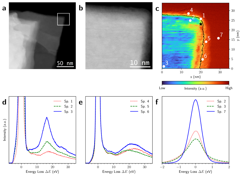
Figure 1: Spatially-resolved EELS analysis of $\text{Bi}_{2}\text{Te}_{3}$. (a) HAADF-STEM image of a representative $\text{Bi}_{2}\text{Te}_{3}$ flake. (b) Magnified region of the top right corner of the specimen around the white square in (a). (c) EELS spectral image corresponding to the white square region in (a). The color map corresponds to the total integrated intensity in each pixel. The black line indicates the edge of the $\text{Bi}_{2}\text{Te}_{3}$ specimen, determined from the thickness map as described in the text. (d) EELS spectra corresponding to the different regions of the specimen indicated in (c): between the vacuum and the edge (sp. $1$); the vicinity of the edge towards the inner region (sp. $2$); and the innermost, thicker part (sp. $3$). Spectra sp. $1$, sp. $2$ and sp. $3$ display the bulk plasmon peak of $\text{Bi}_{2}\text{Te}_{3}$ at around $16$ eV. Additionally, sp. $3$ also shows the Bi $\text{O}_{4,5}$ edges excited from Bi 5$d$ electrons at $25.6$ eV and $27.9$ eV. (e) Same as (d) for EELS spectra in the immediate vicinity of the $\text{Bi}_{2}\text{Te}_{3}$ edge, displaying characteristic features of $\text{Bi}_{2}\text{O}_{3}$. (f) A comparison of sp. 2, sp. 3, and sp. 7 in the low loss and gain regions ($|\Delta E|\leq 2$ eV).

Fig. 1d displays EELS spectra taken at three different locations within the spectral image, labelled as spectra sp$1$, sp$2$, and sp$3$ in the following. Spectra sp$1$, sp$2$, and sp$3$ are acquired in the region between the vacuum and the edge of the specimen, in the vicinity of the specimen edge towards the inner region, and in the innermost part of the specimen, respectively. The three spectra reveal the presence of distinct spectral features located at approximately energy losses of $8.6$ eV and $16.6$ eV, where the latter corresponds to the bulk plasmon peak in accordance with previous studies. [33] Furthermore, the peaks at $25.6$ eV and $27.9$ eV observed in sp$3$ can be identified with the Bi O_4,5 edges excited from Bi 5$d$ electrons, also reported in the literature. [34] Fig. 1e compares three other EEL spectra (labelled as sp$4$, sp$5$, and sp$6$) acquired in the immediate vicinity of the specimen edge. The three spectra exhibit a broad peak located around $21$ eV, which can be identified with the bulk plasmon of $\text{Bi}_{2}\text{O}_{3}$. [35, 36] It is worth nothing that the presence of $\text{Bi}_{2}\text{O}_{3}$ in the surfaces of the specimen is is not visible from the HAADF images. The reason is that HAADF intensity scales with $Z^{n}$, with $Z$ being the atomic number, which is much smaller in O as compared to Te.

Fig. 1f compares the EELS intensities in the region of energy losses $\Delta E$ restricted to the window $\left[-2\leavevmode\nobreak\ {\rm eV},2\leavevmode\nobreak\ {\rm eV}\right]$ for spectra sp$2$, sp$3$, and sp$7$. This comparison illustrates the dependence of the dominant Zero-Loss Peak (ZLP) background with respect to the location in the specimen: bulk (sp$3$), close to edge (sp$2$), and vacuum (sp$7$). On the one hand, as one moves from the vacuum towards the bulk region, the ZLP intensity gradually decreases. This effect can be ascribed to the greater number of inelastic scattering events that occur in the bulk (thicker) regions, compared to the vacuum where the beam electrons do not experience inelastic scatterings. On the other hand, we also observe an enhanced intensity in the specimen regions as compared to the vacuum for $|\Delta E|\geq 0.6$ eV, highlighting material-sensitive contributions to the spectra which contain direct information on its local electronic properties.

Removing this ZLP background is instrumental in order to identify the presence of localised collective excitations such as phonons [24] and plasmon peaks [21] in the low energy-loss region. The same considerations apply to the cleaner energy-gain region [32], where the continuum of inelastic scattering contributions is absent. Here we model the ZLP in terms of a Gaussian distribution following the procedure described in SI-2, with the fitting region restricted to $[-0.4,0.4]$ eV to remove the overlap with $\Delta E$ values at which plasmonic modes of $\text{Bi}_{2}\text{Te}_{3}{}$ have been reported. [9] Subsequently, the ZLP is removed pixel by pixel in the EELS spectral image and the resulting spectra are inspected to identify peaks and other well-defined features in an automated manner. We note that the small band gap [14, 3] of $\text{Bi}_{2}\text{Te}_{3}{}$, $E_{\rm bg}\sim 0.15$ eV, prevents reliably training deep learning models for the ZLP parametrisation and subtraction as done in previous studies from our group. [28, 29, 37] Furthermore, although here we focus on a $\text{Bi}_{2}\text{Te}_{3}{}$ specimen, the procedure is fully general and applicable to other materials which can be inspected with EELS.

Fig. 2 summarises the adopted strategy for the spatially-resolved identification of energy-gain peaks. First, Fig. 2a shows the EEL spectrum for the pixel indicated with a star in Fig. 1c together with the corresponding ZLP fit. Closing up on the energy-gain region, Fig. 2b displays the resulting subtracted spectrum, to which a Lorentzian function is fitted (see SI-2 for details) to extract the position $E_{g}$ and intensity of the dominant energy-gain peak. The procedure is repeated for the complete EELS spectral image, making it possible to construct the spatially-resolved map of $E_{g}$ shown in Fig. 2c across the inspected region of the $\text{Bi}_{2}\text{Te}_{3}{}$ specimen. As in Fig. 1c, the black line indicates the boundary of the $\text{Bi}_{2}\text{Te}_{3}{}$ sample. Fig. 2c reveals the presence of an energy-gain peak in the specimen with $E_{g}$ values between $-1.1$ eV and $-0.85$ eV. We demonstrate in SI-2 that results for the ZLP removal and energy-gain peak identification are robust with respect to the choice of ZLP model function. Then Fig. 2d displays the $\text{Bi}_{2}\text{Te}_{3}{}$ thickness map as obtained from the deconvolution of the single-scattering EELS distribution [28]. The dark blue region beyond the specimen corresponds to either the vacuum or the $\text{Bi}_{2}\text{O}_{3}$ regions. In the edge region there is a sharp increase in thickness, while in the bulk region the thickness exhibits an approximately constant value of 70 nm.

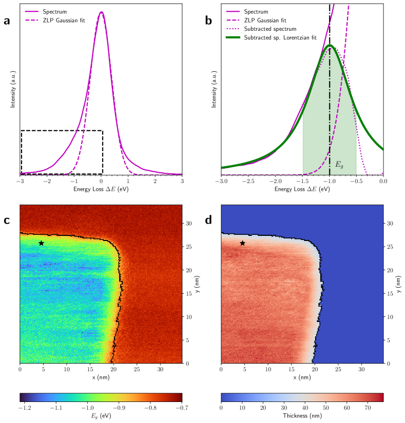
Figure 2: Energy-gain peak identification in $\text{Bi}_{2}\text{Te}_{3}$. (a) The EEL spectrum (solid) in the pixel indicated with a star in Fig. 1c together with the corresponding fit to the ZLP (dashed curve). (b) Close-up of the dashed rectangle in (a), now adding the Lorentzian fit (thick solid line) to the subtracted spectrum (dotted line). The vertical line indicates the mean of the Lorentzian energy-gain peak $E_{g}$, while the filled region indicates the corresponding FWHM. (c) Spatially-resolved map displaying the location of the energy-gain peak $E_{g}$, determined following the procedure of (b) across the whole spectral image of Fig. 1c. (d) Same as (c) now for the local specimen thickness. The dark blue region beyond the specimen edge corresponds to the vacuum region of the spectral image.

In order to further characterise the energy-gain peak identified in Fig. 2c and to correlate its properties with local structural features of the specimen, Figs. 3a and b display the intensity of the ZLP-subtracted EEL spectra integrated in the energy windows $\left[-1.1,-0.6\right]$ eV and $\left[0.6,1.1\right]$ eV for the gain and loss regions respectively. These $\Delta E$ intervals are chosen to contain the range of $E_{g}$ values displayed in Fig. 2c and then mirrored to the energy-loss region. In the latter case, the EEL spectra receive additional contributions to the inelastic scattering distribution beyond those considered here. The most notable feature of Fig. 3a is an enhancement of the integrated intensity in the edge region of the specimen characterised by a sharp variation of the local thickness (Fig. 2d).

Figure 3: Spatially-resolved characterisation of energy-gain peaks. (a) Same as Fig. 1c, now with the intensity of the EEL spectra (after ZLP subtraction) integrated in the window $[-1.1,-0.6]$ eV where the gain peak identified in Fig. 2c is located. (b) Same as (a) for the mirrored energy-loss window, $[0.6,1.1]$ eV. (c) Spatially-resolved map of the ratio $s_{g}$, Eq. (1), defined as the area under the FWHM of the Lorentzian fit to the energy-gain peak, filled region in Fig. 2b, to the area under the ZLP in the same $\Delta E$ window. (d) Ratio of the area $A_{g}$ under the FWHM of the Lorentzian fit to the energy-gain peak to its counterpart $A_{\ell}$ in the loss region, where the vacuum region is masked out for clarity.

To quantify the statistical significance of the identified energy-gain peak, it is convenient to evaluate the ratio

$$s_{g}\equiv\left(A_{g}/A_{\rm zlp}\right)_{\rm g-fwhm}\,,$$ (1)

where $A_{g}$ and $A_{\rm zlp}$ are defined as the areas under the full width at half-maximum (FWMH) of the Lorentzian fit signal, filled region in Fig. 2b, and under the ZLP in the same $\Delta E$ region, respectively. In other words, $s_{g}$ measures the significance of the energy-gain peak in units of the ZLP background. Fig. 3c displays a spatially-resolved map of $s_{g}$ across the specimen. The region of enhanced intensity reported in Fig. 3a and associated to the specimen edge corresponds to the highest values of $s_{g}$ in Fig. 3c, reaching up to a factor two. This high significance confirms that the observe intensity enhancement in the gain region is a genuine feature of the data rather than an artifact of the ZLP removal procedure.

It is also interesting to compare the features of the approximately symmetric peaks appearing in the energy-gain and energy-loss regions, whose values $E_{g}$ and $E_{\ell}$ respectively are mapped across the specimen in Fig. 7 of the Supplementary Material. One observes in general a stronger intensity of the energy-gain peak as compared to its energy-loss counterpart. To quantify this observation and to compare their relative intensities, we display in Fig. 3d the ratio $A_{g}/A_{\ell}$ of the areas under the FWHM of the energy-gain Lorentzian fit to that of the energy-loss peak. The vacuum region is masked out to facilitate readability. As can be seen, in the bulk of the sample the ratio $A_{g}/A_{\ell}$ is of the order unity, whereas in the edge region of the specimen the ratio reaches a factor of around 4. The latter result indicates that surface and edge effects enhance the relative intensity of the energy-gain peak. The combination pf Figs. 2 and 3 demonstrates the presence of a well-defined, significant energy-gain peak in $\text{Bi}_{2}\text{Te}_{3}{}$ located around $E_{g}\simeq-0.9$ eV whose intensity is enhanced in the edge regions of the specimen close to the boundary.

A potential limitation of this analysis concerns the lack of a systematic estimate of the functional uncertainties associated to the ZLP modelling and its subsequent subtraction from the EELS spectral image. To this purpose, we deploy the Monte Carlo replica method for error propagation, originally developed for proton structure studies in high-energy physics [38, 39, 40, 41, 42] and then extended to deep learning models of the ZLP within the EELSfitter framework. [28, 29] First, one applies $K$-means clustering to the EELS spectral image with the similarity measure being the area under the three bins of the EELS intensity around $\Delta E=0$, which operates as a proxy for the local thickness map of Fig. 2d. This procedure results in the 20 clusters shown in Fig. 4a, each of them composed by pixels with similar thickness. Within each cluster, the EELS intensities are assumed to be sampled from the same underlying distribution, and $N_{\mathrm{rep}}$ spectra (“replicas”) are randomly selected from each cluster. By fitting a separate ZLP model to each replica, one ends up with a sampling of $N_{\mathrm{rep}}$ models of the ZLP which can be used to estimate uncertainties and propagate them to the subtracted spectra and the subsequent Lorentzian fits.

Fig. 4b displays the same ZLP-substracted spectrum as in Fig. 2b now with the Monte Carlo replica method used to estimate ZLP model uncertainties. For the ZLP fit, the subtracted spectrum, and the Lorentzian fit to the latter the bands indicate the 68% confidence level (CL) intervals evaluated over the $N_{\rm rep}$ replicas. By repeating this approach in all clusters, we calculate the area ratio $s_{g}$ defined in Eq. (1) for all pixels in the spectral image using the replicas to propagate uncertainties. This results in lower and upper bounds of the 68% confidence interval of the area ratio shown in Fig. 4c and d respectively. The corresponding map of the median of $s_{g}$ is consistent with that reported in Fig. 3c and shown in Fig. 8 in the Supplementary Material. Given that a good significance (above unity) of the energy-gain peak is still observed in the map of the lower limit of the 68% CL interval for the relevant edge region, one can conclude that the results of this work are not distorted by unaccounted-for methodological or procedural uncertainties.

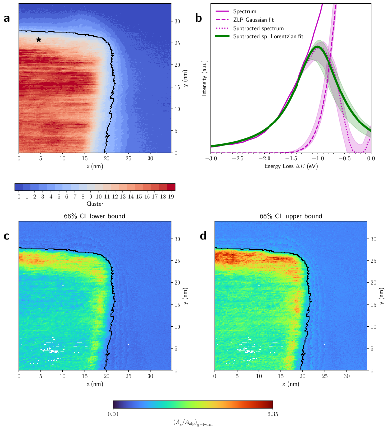
Figure 4: Energy-gain peak characterisation with the Monte Carlo replica method. (a) The EELS spectral image of Fig. 1c classified into 20 clusters, each of them composed by pixels with similar thickness. (b) Same as Fig. 2b now using the Monte Carlo replica method to estimate and propagate the ZLP fitting model uncertainties. For the ZLP Gaussian fit, the subtracted spectrum, and the Lorentzian fit to the latter we display both the median over replicas and the 68% CL intervals. (c,d) Same as Fig. 3c now the lower and upper ranges, respectively, of the 68% CL interval for the area ratio evaluated over the Monte Carlo replicas. See Fig. 8 in the Supplementary Material for the corresponding median map.

To confirm the reproducibility of our findings, we have performed additional measurements on a different $\text{Bi}_{2}\text{Te}_{3}$ specimen characterised by the same crystal structure and with comparable features as the one discussed here. The resulting analysis is summarised in SI-5 of the Supplementary Material and reveals the same qualitative features in the energy-gain region, namely a well-defined, narrow peak at energy gains around $-0.7$ eV whose intensity is enhanced in edge and surface regions and whose significance reaches values of $s_{g}\sim 4$. This independent analysis further confirms the robustness of our results, in particular the strong correlation between the enhanced intensity of the energy-gain peak located around $[-0.9,-0.7]$ eV and specimen regions displayed sharp thickness variations including edges and surfaces.

It is beyond our scope to identify the underlying physical phenomena leading to the observed edge- and surface-induced energy-gain peaks in $\text{Bi}_{2}\text{Te}_{3}{}$. Several mechanisms have been explored leading to resonance signatures in the $\Delta E$ region relevant for our results, such as wedge Dyakonov waves [43] and edge- and surface-located Dirac-plasmons in the closely related TI material Bi₂Se₃. One can in any case exclude thermal effects associated to a Bose-Einstein distribution, given that states with $\sim 1$ eV have a very low occupation probability at room temperatures. Disentangling the specific mechanisms explaining our observations requires dedicated theoretical simulations mapping the EELS response of $\text{Bi}_{2}\text{Te}_{3}{}$ with different structural and geometric configurations and is left for future work.

Summary and Outlook

In this work we have presented a systematic, spatially-resolved investigation of the energy-gain region of EELS spectral images acquired on Bi₂Te₃ specimens. The main motivation was to avoid the inelastic continuum that pollutes the energy-loss region, which may prevent identifying exotic phenomena appearing at $\Delta E$ values below a few eV. An automated peak-identification procedure identifies a narrow feature located around $\Delta E\sim-0.8$ eV whose intensity and significance are strongly enhanced in regions characterised by sharp thickness variations, such as surfaces and edges. We assess the role of methodological uncertainties associated to e.g. the ZLP subtraction procedure and find that our results are robust against them. The observed resonance could be the signature of edge- and surface-plasmons such as those reported in Bi₂Se₃, thought dedicated simulations would be required to unambiguously ascertain its origin.

While here we focus in $\text{Bi}_{2}\text{Te}_{3}{}$ as a proof-of-concept, our approach for ZLP substraction and energy-gain peak tracking is fully general and can be deployed to any specimen for which EELS-SI measurements are acquired, and in particular it is amenable to atomically thin materials of the van der Waals family. Our approach is made available in the new release of the EELSfitter framework and hence can be straightforwardly used by other researchers aiming to explore the information contained in the energy-gain region of EELS-SI to identify, model, and correlate localised collective excitations in nanostructured materials. Possible future improvements include the extension to multiple gain-peaks deconvolution and the improved modelling of the loss region describing the inelastic continuum background. All in all, our findings illustrate the powerful reach of energy-gain EELS to accurately map and characterise the signatures of collective excitations and other exotic resonances arising in quantum materials.

Methods

Specimen preparation. The specimen used in this study were $\text{Bi}_{2}\text{Te}_{3}$ flakes that were mechanically exfoliated from bulk crystals through sonication in isopropanol (IPA) at a ratio of $2$ mg of $\text{Bi}_{2}\text{Te}_{3}$ per $1$ ml of IPA. The exfoliated flakes were then transferred onto holey carbon grids for EELS investigations.

STEM-EELS settings. The scanning transmission electron microscopy (STEM) images and electron energy-loss/gain spectra were obtained using a JEOL200F monochromated equipped with aberration corrector and a Gatan Imaging Filter (GIF) continuum spectrometer. The instrument was operated at $200$ kV and the convergence semi-angle was $14$ mrad. The collection semi-angle for EELS acquisition was $18.3$ mrad obtained by inserting a $5$ mm EELS entrance aperture. The EELS dispersion was $50$ meV per channel.

Data processing and interpretation. The spatially-resolved maps of the energy-gain peaks and the associated peak identification, fitting, and data analysis techniques were performed using the open-source Python package EELSfitter. All features presented in this work are available in its latest public release together with the accompanying input EELS spectral images via its GitHub repository.

Declaration of Competing Interest

The authors declare that they have no known competing financial interests or personal relationships that could have appeared to influence the work reported in this paper.

Funding

H. L., A. B., and S.C.-B. acknowledge financial support from ERC through the Starting Grant “TESLA” grant agreement no. 805021. The work of J. R. is partially supported by NWO (Dutch Research Council) and by an ASDI (Accelerating Scientific Discoveries) grant from the Netherlands eScience Center. The work of J. t. H is supported by NWO (Dutch Research Council).

Supplementary Material

The supplementary material of this manuscript provides technical details on the atomic structure characterisation of $\text{Bi}_{2}\text{Te}_{3}{}$, the energy-gain peak identification procedure, the uncertainty estimate using the Monte Carlo replica method, and the analysis of the energy-gain peaks in different $\text{Bi}_{2}\text{Te}_{3}{}$ specimens.

1 Atomic structure characterisation of $\text{Bi}_{2}\text{Te}_{3}{}$

Fig. 5 presents the STEM analysis of the $\text{Bi}_{2}\text{Te}_{3}{}$ specimen considered in the main manuscript. Fig. 5a shows a low-magnification high-angle annular dark-field (HAADF) STEM image taken on the same $\text{Bi}_{2}\text{Te}_{3}{}$ crystal inspected by EELS. The corresponding atomic-resolution HAADF-STEM image of the region indicated with a blue square in Fig. 5a is displayed in Fig. 5b. As well known, $\text{Bi}_{2}\text{Te}_{3}{}$ is characterised by a hexagonal primitive cell. From the corresponding fast Fourier transform (FFT), Fig. 5c, it is found that this $\text{Bi}_{2}\text{Te}_{3}{}$ crystal is oriented along the $[-1\leavevmode\nobreak\ 1\leavevmode\nobreak\ 1]$ direction. Fig. 5d shows an atomic model of the $\text{Bi}_{2}\text{Te}_{3}{}$ crystal viewed along the same $[-1\leavevmode\nobreak\ 1\leavevmode\nobreak\ 1]$ direction, displaying the characteristic hexagonal crystal structure of $\text{Bi}_{2}\text{Te}_{3}{}$.

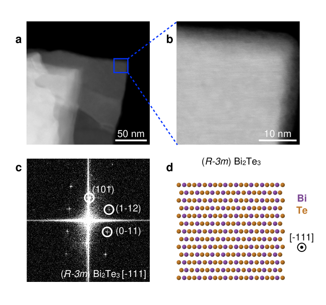
Figure 5: STEM analysis of the $\text{Bi}_{2}\text{Te}_{3}{}$ crystal analysed. (a) Low-magnification HAADF-STEM image of the $\text{Bi}_{2}\text{Te}_{3}{}$ specimen considered in this work. (b) Atomic-resolution HAADF-STEM image of the region indicated with a blue squared in (a). The $\text{Bi}_{2}\text{Te}_{3}{}$ crystal is oriented along the $[-1\leavevmode\nobreak\ 1\leavevmode\nobreak\ 1]$ direction, as shown in the corresponding Fast Fourier transform (FFT) in (c). (d) Atomic model of the $\text{Bi}_{2}\text{Te}_{3}{}$ crystal viewed along the $[-1\leavevmode\nobreak\ 1\leavevmode\nobreak\ 1]$ direction.

2 Peak identification procedure

Here we describe the procedure used to identify and characterise energy-gain peaks in $\text{Bi}_{2}\text{Te}_{3}{}$. We demonstrate how our approach is robust with respect to the model adopted for the ZLP. As mentioned in the main manuscript, while here we focus on a $\text{Bi}_{2}\text{Te}_{3}{}$ specimen, our energy-gain peak identification algorithm is general and could be applied to other materials.

The results presented in the main manuscript are based on a Gaussian model for the ZLP,

$$I_{\rm ZLP}(\Delta E)=I_{\rm ZLP}^{(\rm max)}\exp{\left(-\frac{(\Delta E-\Delta E_{0})^{2}}{2\sigma^{2}}\right)}\,,$$ (2)

with $\Delta E$ being the energy loss (and hence $\Delta E<0$ implies energy gains), $\Delta E_{0}$ and $\sigma^{2}$ being the mean and variance of the distribution, and $I^{(\rm max)}_{\rm ZLP}$ is the maximal intensity of the ZLP. This Gaussian model for the ZLP, Eq. (2), is fitted independently to each individual spectra composing the spectral image. The fit region is restricted to $[-0.4,0.4]$ eV in order to remove the possible overlap with those values of $\Delta E$ at which plasmonic modes of $\text{Bi}_{2}\text{Te}_{3}{}$ have been previously reported. Subsequently, the ZLP Gaussian model Eq. (2) is removed from the measured spectral image and the resulting subtracted spectra are inspected to identify peaks or other relevant features in a fully automated manner.

In this work we identify energy-gain peaks by fitting the subtracted spectra in the energy region $[-3.5,-0.4]$ eV with a Lorentzian function given by

$$I_{\text{peak}}(\Delta E)=I_{\max}\,\frac{\Gamma^{2}}{\Gamma^{2}+(\Delta E-E_{g})^{2}}$$ (3)

where $I_{\max}$ is the height of the peak, $\Gamma$ its width, and $E_{g}$ its median, the latter corresponding to the most likely location of the peak being identified. Once one has determined the parameters of the Lorentzian model Eq. (3) for each of the pixels composing the spectral image, we can determine relevant estimators such as the FWHM and the area underneath it. This way, it is possible to determine the statistical significance of the observed features. Although in this work we consider only single-peak identification, in the presence of multiple features in the energy-gain region Eq. (3) could be extended to a sum of a series of independent Lorentzian resonances.

The robustness of the results presented in this work upon variations of the model assumed for the ZLP is demonstrated by repeating the analysis using other functional forms for the ZLP model. Specifically, in addition to the Gaussian model Eq. (2) we consider a split Gaussian function, a Pearson VII function, and a Pseudo-Voigt function to parameterise the ZLP, all other aspects of the fitting procedure unchanged. These three models are described below and have been considered in the EELS literature in the context of the ZLP subtraction.

Split Gaussian function.

This model is the same as the Gaussian function of Eq. (2) with the difference that the variance is different at the left side and at the right side of the peak. An asymmetric model such a split Gaussian may be more adequate to describe the ZLP in the presence of an intrinsic asymmetry in the energy loss $\Delta E$.

Pearson VII function.

This function is often used to describe peak shapes from $X$-ray powder diffraction patterns [44] and is defined as

$$I(\Delta E)=I_{\max}\frac{w^{2m}}{\left[w^{2}+\left(2^{1/m}-1\right)\left(\Delta E-\Delta E_{0}\right)^{2}\right]^{m}}\,,$$ (4)

with $w$ defining the peak width. The model parameter $m$ can be adjusted and here we find that $m=4$ provides the best description of the ZLP.

The pseudo-Voigt function.

The Voigt function is defined as the convolution of two broadening functions, one a Gaussian and the other a Lorentzian function. The pseudo-Voigt function is also a popular choice in describing peak shapes in diffraction patterns [45] and approximates the exact convolution by a linear combination of a Gaussian and a Lorentzian. Their mixing can be adjusted by a model parameter $\eta$ as follows:

$$I(\Delta E)=I_{\max}\left[\eta G\left(\Delta E,\sigma^{2}\right)+\left(1-\eta\right)L\left(\Delta E,\sigma^{2}\right)\right],$$ (5)

where $G\left(\Delta E,\sigma^{2}\right)$ and $L\left(\Delta E,\sigma^{2}\right)$ are normalised Gaussian and Lorentzian functions with a common variance $\sigma^{2}$ respectively.

Stability upon choice of ZLP model.

Fig. 6 displays, as done in Fig. 3a of the main manuscript, the ZLP-subtracted EELS intensity integrated in the region $[-1.1,-0.6]$ eV around the identified energy-gain peak. We compare the outcome of our baseline choice, a Gaussian model for the ZLP (a), with the corresponding results based on (b) split Gaussian, (c) Pearson VII, and (d) pseudo-Voigt functions for the ZLP parametrisation. Each panel adopts its own intensity range, and similar colors in the different panels in general do not correspond to similar intensity values. Irrespective of the choice of ZLP model function, the highest integrated intensity is found in the edge region of the specimen. We have verified that other relevant properties of the energy-gain peak at $\Delta E\simeq-1$ eV, such as its mean and width, are also stable with respect to this choice. We conclude that our energy-gain peak identification algorithm is robust with respect to the modelling of the ZLP.

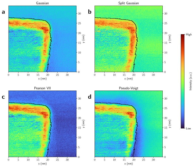
Figure 6: Same as Fig. 3a in the main manuscript, displaying the ZLP-subtracted EELS intensity integrated in the region $[-1.1,-0.6]$ eV around the identified energy-gain peak. We compare the outcome of our baseline choice, a Gaussian model for the ZLP (a), with the corresponding results based on (b) split Gaussian, (c) Pearson VII, and (d) pseudo-Voigt functions for the ZLP parametrisation. Each panel adopts its own intensity range, and similar colors in the different panels in general do not correspond to similar intensity values. Irrespective of the choice of ZLP model function, the highest integrated intensities are found near the edge region indicated by a black curve.

3 Peak location in the energy-loss region

Fig. 2c in the main manuscript displays a spatially-resolved map with the value of $E_{g}$, the median of the Lorentzian peak fitted to the ZLP-subtracted energy-gain region. For completeness, we show in Fig. 7b the same map now for $E_{\ell}$, the median of the Lorentzian peak fitted to the ZLP-subtracted energy-loss region. We emphasize that our model for the energy-loss region is incomplete, given that the data contains additional contributions beyond this dominant peak.

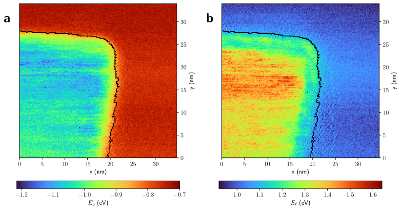
Figure 7: (a) Same as Fig. 2c. (b) Same as Fig. 2c now displaying the value of $E_{\ell}$, the median of the Lorentzian peak fitted to the ZLP-subtracted energy-loss region.

In the region of the specimen where the energy-gain peak exhibits the highest significance, namely close to the edge, the value of the fitted energy-loss peak is $E_{\ell}\sim$1 eV, corresponding to approximately the energy-mirrored value of its energy-gain counterpart. However, the significance of this energy-loss feature is weaker, see Fig. 3d, and only with a complete model of the energy-loss region would it be possible to robustly disentangle the different energy-loss features present in the considered specimen.

4 Uncertainty estimate using the Monte Carlo replica method

The lower and upper 68% confidence level intervals computed on the ratio between the area within the FWHM of the gain peak and that of the ZLP in the same $\Delta E$ region, estimated from the spread of the Monte Carlo replicas, were already showed in the bottom panels of Fig. 4. In Fig. 8, for completeness, we also report on the corresponding spatially-resolved map for the median of this 68% CL interval. The qualitative agreement between panels a,b,c of Fig. 8 indicate that uncertainties associated to the ZLP modelling and substraction procedure are moderate and do not distort the main results obtained in this work.

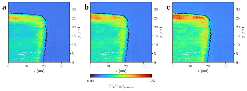
Figure 8: Spatially-resolved map of the lower 68% CL bound (a), median (b), and upper 68% CL bound (c) of the ratio between the area within the FWHM of the gain peak and that of the ZLP in the same $\Delta E$ region, estimated from the spread of the Monte Carlo replicas. The lower and upper bounds were already showed in the bottom panels of Fig. 4 and are repeated here for completeness.

5 Energy-gain peaks in different $\text{Bi}_{2}\text{Te}_{3}{}$ specimens

While the results presented in the main manuscript consider the EELS analysis of a specific $\text{Bi}_{2}\text{Te}_{3}{}$ specimen, we found that consistent results are obtained in other comparable specimens. In the following, the microscope parameters that were used are the same as the ones mentioned in the Methods section of the main manuscript.

Fig. 9a shows an HAADF image of another $\text{Bi}_{2}\text{Te}_{3}{}$ specimen, different from the one in the main manuscript, and characterised by the presence of a channel, indicated by the darker contrast. Fig. 9b focuses on the region above the channel which is subsequently analysed with electron energy-gain spectroscopy. This region is composed by a flat layer alongside some edges. The channel region is characterised by sharp variations of the specimen thickness, which motivate the inspection of the specimen for edge- and surface-induced excitations.

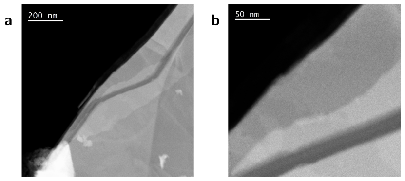
Figure 9: (a) HAADF image of another $\text{Bi}_{2}\text{Te}_{3}{}$ specimen, characterised by the presence of a channel (darker contrast). (b) A zoomed-in image of the same specimen, focusing on the region above the channel which is analysed by means of EELS.

Figs. 10 and 11 present the same spatially-resolved electron energy-gain analyses of Figs. 2 and 3 in the main manuscript respectively, now corresponding to the $\text{Bi}_{2}\text{Te}_{3}{}$ specimen displayed in Fig. 9. The black line indicates the specimen boundary, and pixels in which the fitting procedure is numerically unstable are masked out. An enhancement of the intensity in the $\Delta E$ gain region located around $-0.7$ eV is observed in specific regions of the sample, as illustrated by the representative spectrum in Fig. 10b corresponding to the location marked with a star in Fig. 10a. This feature is most prominent in the region above the channel identified in Fig. 9 and close to the specimen surface. No equivalent enhancement is observed in the loss region, where it could be confounded by other mechanisms contributing to energy-loss inelastic scatterings.

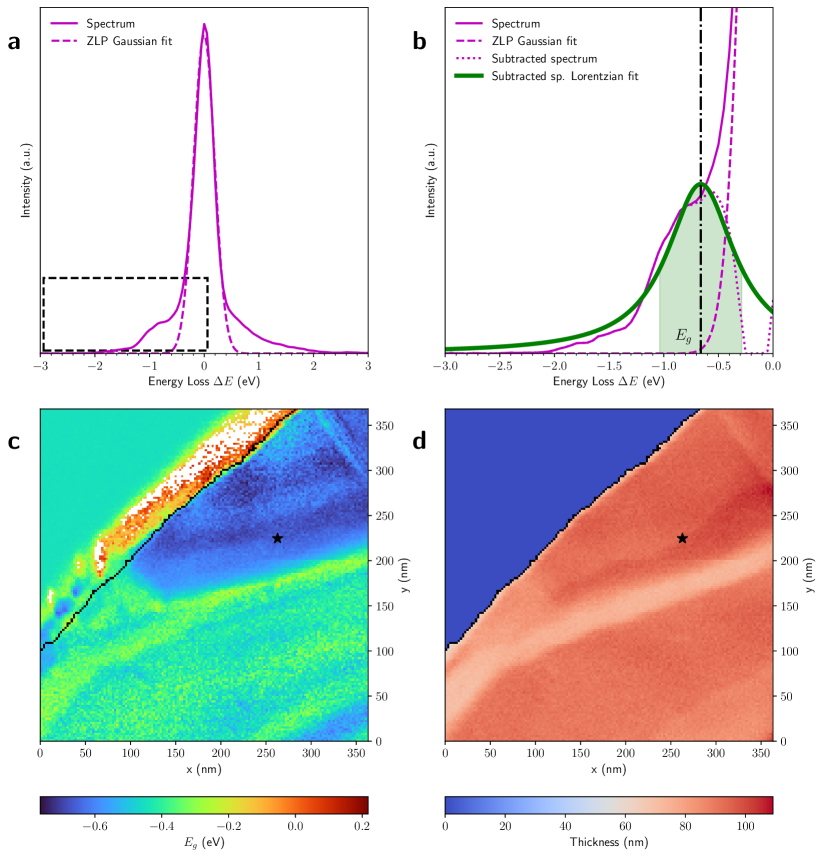
Figure 10: Same as Fig. 2 in the main manuscript for a different $\text{Bi}_{2}\text{Te}_{3}{}$ crystal. The star indicates the location in the specimen in which the individual EEL spectrum of (a) and (b) is extracted.

Applying the same peak identification procedure used for the specimen in the main manuscript and further detailed in Sect. 2, we find that in the region where the energy gain peak is more marked the center of the Lorentzian is located around $\Delta E=-0.7$ eV, see Fig. 10d for the associated spatially-resolved map. Integrating in the energy gain region defined by the window $[-1.1,-0.6]$ eV the intensity is highest in the region just above the channel, Fig. 11a. The ratio of the area under the FWHM of the Lorentzian peak over that under the ZLP, Fig. 11c, is also enhanced in the same region, where it takes values between $2$ and $3.5$. In the region of the specimen with the highest signal-to-noise significance, the position of the Lorentzian median is approximately constant and takes value $E_{g}\sim-0.7$ eV. We verify, by means of the same procedure adopted for Fig. 6, that our results are independent of the specific choice of functional form model for the ZLP.

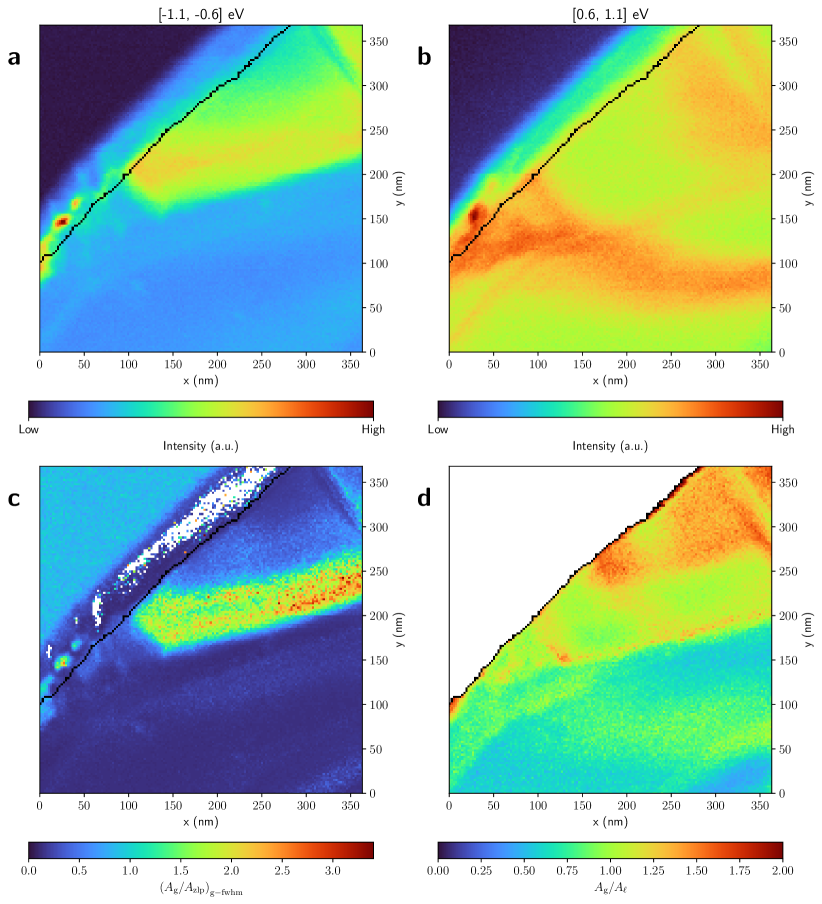
Figure 11: Same as Fig. 3 in the main manuscript for the same $\text{Bi}_{2}\text{Te}_{3}{}$ crystal analysed in Fig. 10.

The analysis presented here, performed on a different $\text{Bi}_{2}\text{Te}_{3}{}$ specimen but with the same crystal structure and comparable features as that of the main manuscript, confirms the robustness of our characterisation of the energy gain region of $\text{Bi}_{2}\text{Te}_{3}{}$, establishing the presence of a distinctive gain peak located in the region around $\Delta E=-0.7$ eV. This feature can be disentangled from the dominant ZLP emission with high significance and is also found to be enhanced in the regions of the specimen displaying sharp thickness variations with the associated exposed surfaces and edges.

References

- [1] Zhang, H. et al. Topological insulators in Bi2Se3, Bi2Te3 and Sb2Te3 with a single Dirac cone on the surface. \JournalTitleNat. Phys. 5, 438–442, DOI: 10.1038/nphys1270 (2009).
- [2] Xia, Y. et al. Observation of a large-gap topological-insulator class with a single Dirac cone on the surface. \JournalTitleNat. Phys. 5, 398–402, DOI: 10.1038/nphys1274 (2009).
- [3] Hsieh, D. et al. Observation of Time-Reversal-Protected Single-Dirac-Cone Topological-Insulator States in and . \JournalTitlePhys. Rev. Lett. 103, 146401, DOI: 10.1103/PhysRevLett.103.146401 (2009).
- [4] Grigorenko, A. N., Polini, M. & Novoselov, K. S. Graphene plasmonics. \JournalTitleNature Photonics 6, 749–758, DOI: 10.1038/nphoton.2012.262 (2012).
- [5] Di Pietro, P. et al. Observation of Dirac plasmons in a topological insulator. \JournalTitleNature Nanotechnology 8, 556–560, DOI: 10.1038/nnano.2013.134 (2013).
- [6] Autore, M. et al. Plasmon–phonon interactions in topological insulator microrings. \JournalTitleAdvanced Optical Materials 3, 1257–1263, DOI: https://doi.org/10.1002/adom.201400513 (2015). https://onlinelibrary.wiley.com/doi/pdf/10.1002/adom.201400513.
- [7] Yin, J. et al. Plasmonics of topological insulators at optical frequencies. \JournalTitleNPG Asia Materials 9, e425–e425, DOI: 10.1038/am.2017.149 (2017).
- [8] Giorgianni, F. et al. Strong nonlinear terahertz response induced by dirac surface states in bi2se3 topological insulator. \JournalTitleNature communications 7, 11421, DOI: https://doi.org/10.1038/ncomms11421 (2016).
- [9] Zhao, M. et al. Visible Surface Plasmon Modes in Single Bi2Te3 Nanoplate. \JournalTitleNano Letters 15, 8331–8335, DOI: 10.1021/acs.nanolett.5b03966 (2015).
- [10] Whitcher, T. J. et al. Correlated plasmons in the topological insulator bi2se3 induced by long-range electron correlations. \JournalTitleNPG Asia Materials 12, 37, DOI: 10.1038/s41427-020-0218-7 (2020).
- [11] Kitaev, A. & Preskill, J. Topological Entanglement Entropy. \JournalTitlePhys. Rev. Lett. 96, 110404, DOI: 10.1103/PhysRevLett.96.110404 (2006).
- [12] Fu, L. & Kane, C. L. Superconducting Proximity Effect and Majorana Fermions at the Surface of a Topological Insulator. \JournalTitlePhys. Rev. Lett. 100, 096407, DOI: 10.1103/PhysRevLett.100.096407 (2008).
- [13] Zhang, X., Wang, J. & Zhang, S.-C. Topological insulators for high-performance terahertz to infrared applications. \JournalTitlePhys. Rev. B 82, 245107, DOI: 10.1103/PhysRevB.82.245107 (2010).
- [14] Chen, Y. L. et al. Experimental Realization of a Three-Dimensional Topological Insulator, Bi2Te3. \JournalTitleScience 325, 178–181, DOI: 10.1126/science.1173034 (2009). https://www.science.org/doi/pdf/10.1126/science.1173034.
- [15] Chu, M.-W. et al. Probing bright and dark surface-plasmon modes in individual and coupled noble metal nanoparticles using an electron beam. \JournalTitleNano Letters 9, 399–404, DOI: 10.1021/nl803270x (2009).
- [16] García de Abajo, F. J. Optical excitations in electron microscopy. \JournalTitleRev. Mod. Phys. 82, 209–275, DOI: 10.1103/RevModPhys.82.209 (2010).
- [17] Myroshnychenko, V. et al. Plasmon spectroscopy and imaging of individual gold nanodecahedra: A combined optical microscopy, cathodoluminescence, and electron energy-loss spectroscopy study. \JournalTitleNano Letters 12, 4172–4180, DOI: 10.1021/nl301742h (2012).
- [18] Coenen, T. et al. Nanoscale spatial coherent control over the modal excitation of a coupled plasmonic resonator system. \JournalTitleNano Letters 15, 7666–7670, DOI: 10.1021/acs.nanolett.5b03614 (2015).
- [19] Nerl, H. C. et al. Probing the local nature of excitons and plasmons in few-layer mos2. \JournalTitlenpj 2D Materials and Applications 1, 2, DOI: 10.1038/s41699-017-0003-9 (2017).
- [20] Lagos, M. J., Trügler, A., Hohenester, U. & Batson, P. E. Mapping vibrational surface and bulk modes in a single nanocube. \JournalTitleNature 543, 529–532, DOI: 10.1038/nature21699 (2017).
- [21] Yankovich, A. B. et al. Visualizing spatial variations of plasmon–exciton polaritons at the nanoscale using electron microscopy. \JournalTitleNano Letters 19, 8171–8181, DOI: 10.1021/acs.nanolett.9b03534 (2019).
- [22] Krivanek, O. L. et al. Vibrational spectroscopy in the electron microscope. \JournalTitleNature 514, 209–212, DOI: 10.1038/nature13870 (2014).
- [23] Egoavil, R. et al. Atomic resolution mapping of phonon excitations in stem-eels experiments. \JournalTitleUltramicroscopy 147, 1–7, DOI: https://doi.org/10.1016/j.ultramic.2014.04.011 (2014).
- [24] Govyadinov, A. A. et al. Probing low-energy hyperbolic polaritons in van der waals crystals with an electron microscope. \JournalTitleNature Communications 8, 95, DOI: 10.1038/s41467-017-00056-y (2017).
- [25] Venkatraman, K., Levin, B. D. A., March, K., Rez, P. & Crozier, P. A. Vibrational spectroscopy at atomic resolution with electron impact scattering. \JournalTitleNature Physics 15, 1237–1241, DOI: 10.1038/s41567-019-0675-5 (2019).
- [26] Hage, F. S., Radtke, G., Kepaptsoglou, D. M., Lazzeri, M. & Ramasse, Q. M. Single-atom vibrational spectroscopy in the scanning transmission electron microscope. \JournalTitleScience 367, 1124–1127, DOI: 10.1126/science.aba1136 (2020).
- [27] Qi, R. et al. Four-dimensional vibrational spectroscopy for nanoscale mapping of phonon dispersion in bn nanotubes. \JournalTitleNature Communications 12, 1179, DOI: 10.1038/s41467-021-21452-5 (2021).
- [28] Brokkelkamp, A. et al. Spatially Resolved Band Gap and Dielectric Function in Two-Dimensional Materials from Electron Energy Loss Spectroscopy. \JournalTitleThe Journal of Physical Chemistry A 126, 1255–1262, DOI: 10.1021/acs.jpca.1c09566 (2022).
- [29] Roest, L. I., van Heijst, S. E., Maduro, L., Rojo, J. & Conesa-Boj, S. Charting the low-loss region in electron energy loss spectroscopy with machine learning. \JournalTitleUltramicroscopy 222, 113202, DOI: https://doi.org/10.1016/j.ultramic.2021.113202 (2021).
- [30] Boersch, H., Geiger, J. & Stickel, W. Interaction of 25-kev electrons with lattice vibrations in lif. experimental evidence for surface modes of lattice vibration. \JournalTitlePhys. Rev. Lett. 17, 379–381, DOI: 10.1103/PhysRevLett.17.379 (1966).
- [31] Asenjo-Garcia, A. & de Abajo, F. J. G. Plasmon electron energy-gain spectroscopy. \JournalTitleNew Journal of Physics 15, 103021, DOI: 10.1088/1367-2630/15/10/103021 (2013).
- [32] Idrobo, J. C. et al. Temperature measurement by a nanoscale electron probe using energy gain and loss spectroscopy. \JournalTitlePhys. Rev. Lett. 120, 095901, DOI: 10.1103/PhysRevLett.120.095901 (2018).
- [33] Peranio, N. et al. Low loss eels and eftem study of bi2te3 based bulk and nanomaterials. \JournalTitleMRS Online Proceedings Library (OPL) 1329, mrss11–1329–i10–21, DOI: 10.1557/opl.2011.1238 (2011).
- [34] Nascimento, V. et al. Xps and eels study of the bismuth selenide. \JournalTitleJournal of Electron Spectroscopy and Related Phenomena 104, 99–107, DOI: https://doi.org/10.1016/S0368-2048(99)00012-2 (1999).
- [35] Torruella, P. et al. Assessing oxygen vacancies in bismuth oxide through eels measurements and dft simulations. \JournalTitleThe Journal of Physical Chemistry C 121, 24809–24815, DOI: 10.1021/acs.jpcc.7b06310 (2017).
- [36] Li, Y. et al. Plasmonic hot electrons from oxygen vacancies for infrared light-driven catalytic co2 reduction on bi2o3-x. \JournalTitleAngewandte Chemie International Edition 60, 910–916, DOI: https://doi.org/10.1002/anie.202010156 (2021). https://onlinelibrary.wiley.com/doi/pdf/10.1002/anie.202010156.
- [37] van Heijst, S. E. et al. Illuminating the electronic properties of ws2 polytypism with electron microscopy. \JournalTitleAnnalen der Physik 533, 2000499, DOI: https://doi.org/10.1002/andp.202000499 (2021). https://onlinelibrary.wiley.com/doi/pdf/10.1002/andp.202000499.
- [38] Watt, G. & Thorne, R. S. Study of Monte Carlo approach to experimental uncertainty propagation with MSTW 2008 PDFs. \JournalTitleJ. High Energy Phys. 2012, 52–38, DOI: 10.1007/JHEP08(2012)052 (2012).
- [39] The NNPDF Collaboration et al. Neural network determination of parton distributions: the nonsinglet case. \JournalTitleJournal of High Energy Physics 2007, 039, DOI: 10.1088/1126-6708/2007/03/039 (2007).
- [40] Ball, R. D. et al. Parton distributions for the LHC Run II. \JournalTitleJHEP 04, 040, DOI: 10.1007/JHEP04(2015)040 (2015). 1410.8849.
- [41] Hartland, N. P. et al. A Monte Carlo global analysis of the Standard Model Effective Field Theory: the top quark sector. \JournalTitleJHEP 04, 100, DOI: 10.1007/JHEP04(2019)100 (2019). 1901.05965.
- [42] Candido, A. et al. Neutrino Structure Functions from GeV to EeV Energies. \JournalTitleJHEP 2302.08527.
- [43] Talebi,, N. et al. Wedge Dyakonov Waves and Dyakonov Plasmons in Topological Insulator Bi2Se3 Probed by Electron Beams. \JournalTitleACS nano 10, 6988, DOI: https://doi.org/10.1021/acsnano.6b02968 (2016).
- [44] “Peak Shape Functions: Pearson VII.” Birkbeck College, University of London, http://pd.chem.ucl.ac.uk/pdnn/peaks/pvii.htm, 2006.
- [45] “Peak Shape Functions: Pseudo-Voigt and Other Functions.” Birkbeck College, University of London, http://pd.chem.ucl.ac.uk/pdnn/peaks/others.htm, 2006.
Supporting Information: