The interpretation of present and future neutrino experiments requires accurate theoretical predictions for neutrino-nucleus scattering rates. Neutrino structure functions can be reliably evaluated in the deep-inelastic scattering regime within the perturbative QCD (pQCD) framework. At low momentum transfers ($Q^{2}\mathrel{\hbox to0.0pt{\lower 4.0pt\hbox{\hskip 1.0pt$\sim$}\hss}\raise 1.0pt\hbox{$<$}}{\rm few}$ GeV²), inelastic structure functions are however affected by large uncertainties which distort event rate predictions for neutrino energies $E_{\nu}$ up to the TeV scale. Here we present a determination of neutrino inelastic structure functions valid for the complete range of energies relevant for phenomenology, from the GeV region entering oscillation analyses to the multi-EeV region accessible at neutrino telescopes. Our NNSF$\nu$ approach combines a machine-learning parametrisation of experimental data with pQCD calculations based on state-of-the-art analyses of proton and nuclear parton distributions (PDFs). We compare our determination to other calculations, in particular to the popular Bodek-Yang model. We provide updated predictions for inclusive cross sections for a range of energies and target nuclei, including those relevant for LHC far-forward neutrino experiments such as FASER$\nu$, SND@LHC, and the Forward Physics Facility. The NNSF$\nu$ determination is made available as fast interpolation LHAPDF grids, and it can be accessed both through an independent driver code and directly interfaced to neutrino event generators such as GENIE.

1 Introduction

Precise and reliable theoretical predictions for the scattering rates of (anti-)neutrinos on proton and nuclear targets [1, 2] constitute a central ingredient for the interpretation of a wide variety of ongoing and future neutrino experiments. These include, first of all, oscillation measurements carried out with reactor, accelerator, and atmospheric neutrinos at facilities such as KamLAND [3], DUNE [4], and DeepCore/IceCube-Upgrade [5, 6] and KM3NET-ORCA [7] respectively. Second, neutrino scattering experiments taking place at the CERN complex, from FASER$\nu$ [8, 9], SND@LHC [10], and the Forward Physics Facility (FPF) [11, 12] using LHC neutrinos to SPS beam dump experiments such as SHiP [13]. And third, astroparticle physics analyses involving high- and ultra-high-energy energies [14] at neutrino telescopes such as IceCube [15], KM3NET-ARCA [16], GRAND [17], and POEMMA [18].

Depending on the neutrino energies $E_{\nu}$ involved, different regimes are relevant in the corresponding theoretical calculations. In the sub-GeV region, the dominant interaction process is charged current quasielastic scattering (e.g. $\bar{\nu}_{\mu}p\to\mu^{+}n$), and then as $E_{\nu}$ is increased resonance scattering processes (e.g. $\bar{\nu}_{\mu}n\to\mu^{+}\Lambda^{-}\to\mu^{+}n\pi^{-}$) become the leading contribution. At higher energies and above the resonance region, starting at $E_{\nu}=\mathcal{O}(10)$ GeV and final state invariant masses of $W\mathrel{\hbox to0.0pt{\lower 4.0pt\hbox{\hskip 1.0pt$\sim$}\hss}\raise 1.0pt\hbox{$>$}}2$ GeV, inelastic scattering dominates (e.g. $\bar{\nu}_{\mu}p\to\mu^{+}X$, with $X$ being the hadronic final state). Inelastic neutrino scattering is further divided into shallow inelastic scattering (SIS) and deep-inelastic scattering (DIS) involving momentum transfers $Q^{2}$ below and above the threshold $Q^{2}\simeq{\rm few}$ GeV² which separates the non-perturbative and perturbative regions, respectively. Other interaction processes, typically subdominant but relevant in specific phase space regions, include (in)elastic scattering off the photon field of nucleons, coherent scattering off the photon field of nuclei, and scattering on atomic electrons via the Glashow resonance. Theoretical models of neutrino scattering are implemented in various neutrinos event generators [19], such as GENIE [20, 21] and its high-energy module HEDIS [22], GiBUU [23], and NuWro [24]. Most of these generators are tailored to specific energies and setups and cannot be straightforwardly applied to the whole range of experiments listed above.

Differential cross sections in inelastic neutrino-nucleon scattering are decomposed [25, 26] in terms of structure functions, $F^{\nu A}_{i}(x,Q^{2})$, with $x$ being the Bjorken variable and $Q^{2}$ the momentum transfer squared between the neutrino and the target nucleon. In the DIS regime, these structure functions can be expressed in the framework of perturbative QCD as the factorised convolution of parton distribution functions (PDFs) [27, 28, 29] and hard-scattering partonic cross sections. Their state-of-the-art calculation is based on PDFs and hard-scattering coefficient functions evaluated at next-to-next-to-leading order (NNLO) in the strong coupling $\alpha_{s}$ expansion, with partial and exact [30, 31, 32] results also available one perturbative order higher (N³LO) and used in [33] to extract the proton PDFs. Furthermore, heavy quark (charm, bottom, and top) mass effects can be accounted for by means of general-mass variable-flavour-number (GM-VFN) schemes [34, 35, 36, 37]. In addition, the applicability of fixed-order perturbative QCD calculations can be extended to the large (small) $x$ kinematic region by means of all-order threshold [38] (BFKL[39, 40]) resummation.

While DIS dominates inclusive neutrino-nucleon event rates for energies $E_{\nu}\mathrel{\hbox to0.0pt{\lower 4.0pt\hbox{\hskip 1.0pt$\sim$}\hss}\raise 1.0pt\hbox{$>$}}{\rm few}$ TeV, at lower energies these rates receive a significant contribution from the SIS region. For instance, at $E_{\nu}\sim 100$ GeV up to 20% of the inclusive cross section can arise from the $Q\mathrel{\hbox to0.0pt{\lower 4.0pt\hbox{\hskip 1.0pt$\sim$}\hss}\raise 1.0pt\hbox{$<$}}2$ GeV region [41]. Theoretical predictions of neutrino structure functions in the SIS region are therefore affected by much larger uncertainties than their DIS counterparts, given that they are sensitive to low momentum transfers, $Q^{2}\mathrel{\hbox to0.0pt{\lower 4.0pt\hbox{\hskip 1.0pt$\sim$}\hss}\raise 1.0pt\hbox{$<$}}{\rm few\leavevmode\nobreak\ GeV}^{2}$ [42], where the QCD perturbative and twist expansions break down and the factorisation theorems stop being applicable.

In order to bypass the limitations of perturbative QCD in the SIS region, phenomenological models of low-$Q^{2}$ neutrino structure functions have been developed and implemented in various neutrino event generators. One of the most popular is the Bodek-Yang (BY) model [43, 44, 45, 46, 47, 48], based on structure functions with effective leading-order (LO) PDFs from the GRV98 analysis [49] with modified scaling variables and $K$-factors to approximate mass and higher-order QCD corrections. Drawbacks of the Bodek-Yang approach include the reliance on an obsolete set of PDFs that neglects constraints on the proton and nuclear structure obtained in the last 25 years, ignoring available higher-order QCD calculations, and the lack of a systematic estimate of the uncertainties associated to their predictions. Another restriction of the BY structure functions is that they cannot be consistently matched to calculations of high-energy neutrino scattering based on modern PDFs and higher-order QCD calculations [50, 41, 51, 52, 53], introducing an unnecessary separation between the modelling of neutrino interactions for experiments sensitive to different energy regions.

Here we present the first determination of inelastic neutrino-nucleon structure functions which is valid for the full range of momentum transfers $Q^{2}$ relevant for phenomenology, from oscillation measurements involving multi-GeV neutrinos to ultra-high energy scattering experiments at EeV energies. This determination is based on the NNSF$\nu$ approach, which combines a data-driven machine-learning parametrisation of inelastic structure functions at low and intermediate $Q^{2}$ matched to perturbative QCD calculations at larger $Q^{2}$ values. Following the NNPDF methodology [54, 55, 56, 57, 58, 59, 60, 61], already applied to neutral-current structure functions in [62, 63], neural networks are adopted as universal unbiased interpolants and trained on available accelerator data on neutrino structure functions and differential cross sections, with the Monte Carlo replica method to estimate and propagate uncertainties. The perturbative QCD calculations are provided by YADISM, a new framework for the evaluation of DIS structure functions from the EKO [64] family. Their input is the nNNPDF3.0 determination of nuclear PDFs [65], which reduces in the $A=1$ limit to the proton NNPDF3.1 fit [55], specifically to the variant with LHCb $D$-meson data included [41]. This YADISM perturbative calculation is applicable up to EeV neutrino energies and accounts for exact top mass effects in charged-current scattering.

The NNSF$\nu$ determination hence provides a parametrisation of the structure functions $F_{i}^{\nu A}(x,Q^{2},A)$ ($i=2,3,L$) reliable for arbitrary values of the three inputs $x$, $Q^{2}$, and $A$ together with a comprehensive uncertainty estimate. Our strategy provides a robust estimate of all relevant sources of uncertainty, including those related to experimental errors, functional forms, (nuclear) PDFs, and missing higher order (MHO) uncertainties in the perturbative QCD calculation. We demonstrate the stability of NNSF$\nu$ with respect to variations of both the input data and methodological settings, and show how it correctly inter- and extrapolates for $A$ values not directly constrained in the fit. Upon integration of the structure functions over the kinematically allowed ranges in $x$ and $Q^{2}$, we obtain predictions for inclusive inelastic cross sections, together with the associated uncertainties, without restrictions on the values of the neutrino energy $E_{\nu}$ and mass number $A$ of the target nuclei.

We compare the NNSF$\nu$ structure functions and inclusive cross sections to related calculations available in the literature, in particular to the Bodek-Yang (as implemented in GENIE), BGR18 [41], and CSMS11 [52] predictions. We assess the dependence of our results with respect to the values of $E_{\nu}$ and $A$ and provide dedicated predictions for the energy ranges and target materials relevant for the LHC far-forward neutrino scattering experiments, namely FASER$\nu$, SND@LHC, and the FPF, quantifying in each case the role played by the various sources of uncertainty. The NNSF$\nu$ determination is made available as stand-alone fast interpolation grids in the LHAPDF [66] format which can be accessed either through an independent driver code and or directly interfaced to neutrino event generators such as GENIE. We also provide look-up tables for the inclusive cross sections and their uncertainties as a function of $E_{\nu}$ and $A$.

The outline of this paper is the following. In Sect. 2 we review the theoretical formalism underlying neutrino-nucleus inelastic scattering on proton and nuclear targets, assess the perturbative stability of the QCD calculation, and compare different existing predictions among them. Sect. 3 describes the NNSF$\nu$ approach to construct a data-driven parametrisation of the neutrino structure functions matched to pQCD calculations. Sect. 4 presents the NNSF$\nu$ determination, verifies that it reproduces the input data and theory calculations, studies its robustness and stability, compares it with existing analyses, and evaluates the Gross-Llewellyn Smith sum rule. Predictions for inclusive neutrino cross sections are provided in Sect. 5, in particular we study their $E_{\nu}$ and $A$ dependence, the agreement with experimental data, and the sensitivity to kinematic cuts, and we conclude by outlining some possible future developments in Sect. 6.

Technical details are collected in three appendices. App. A describes the software framework underlying the NNSF$\nu$ determination and how to access and use its results for the inelastic structure functions and cross sections. App. B outlines the main features of the YADISM code used to calculate neutrino structure functions in perturbative QCD and reports the outcome of representative benchmark comparison with APFEL. App. C summarises the impact of nuclear effects in neutrino inelastic scattering at the level of the parton distributions provided by nNNPDF3.0.

2 Neutrino inelastic structure functions

In this section we summarise the theoretical formalism underpinning the evaluation of neutrino-nucleon inelastic scattering cross sections in terms of structure functions and the calculation of the latter in the framework of perturbative QCD. We then present results neutrino structure functions evaluated with YADISM, quantify their perturbative stability and their dependence of the input PDFs, and compare them with the Bodek-Yang and BGR18 predictions.

2.1 DIS structure functions in perturbative QCD

The double-differential cross section for neutrino-nucleus scattering can be decomposed in terms of three independent structure functions $F_{i}^{\nu A}(x,Q^{2})$ with $i=1,2,3$. Focusing on the charged-current (CC) scattering case mediated by the exchange of a $W^{+}$ weak boson, this differential cross section reads

$${{d^{2}\sigma^{\nu A}(x,Q^{2},y)}\over{dxdy}}={{G_{F}^{2}s/2\pi}\over{\left(1+Q^{2}/m_{W}^{2}\right)^{2}}}\left[(1-y)F^{\nu A}_{2}(x,Q^{2})+y^{2}xF^{\nu A}_{1}(x,Q^{2})+y\left(1-{{y}\over{2}}\right)xF^{\nu A}_{3}(x,Q^{2})\right]\,,$$ (2.1)

where $s=2m_{n}E_{\nu}$ is the neutrino-nucleon center of mass energy squared, $m_{n}$ the nucleon mass, $A$ the atomic mass number of the target nucleus, $E_{\nu}$ the incoming neutrino energy, and the inelasticity $y$ is defined as

$$y={{Q^{2}}\over{2xm_{n}E_{\nu}}}={{Q^{2}}\over{xs}}\,.$$ (2.2)

An analogous expression holds for antineutrino scattering, mediated now by the exchange of a $W^{-}$ weak boson, with the only difference being a sign change in front of the parity-violating structure function $xF_{3}$,

$${{d^{2}\sigma^{\bar{\nu}A}(x,Q^{2},y)}\over{dxdy}}={{G_{F}^{2}s/2\pi}\over{\left(1+Q^{2}/m_{W}^{2}\right)^{2}}}\left[(1-y)F^{\bar{\nu}A}_{2}(x,Q^{2})+y^{2}xF^{\bar{\nu}A}_{1}(x,Q^{2})-y\left(1-{{y}\over{2}}\right)xF^{\bar{\nu}A}_{3}(x,Q^{2})\right]\,.$$ (2.3)

While the differential cross sections are a function of three kinematic variables, $(x,Q^{2},y)$, the structure functions themselves depend only on $x$ and $Q^{2}$. Furthermore, both the cross sections and the structure functions depend on the atomic mass number $A$ of the target nucleus only through the nuclear modifications of the free-nucleon structure functions. Kinematic considerations indicate that inelastic structure functions vanish in the elastic limit $x\to 1$, that is,

$$F_{i}^{\nu A}(x=1,Q^{2})=F_{i}^{\bar{\nu}A}(x=1,Q^{2})=0\,,\qquad\forall\,\,i\,.$$ (2.4)

Alternatively, Eq. (2.1) can be expressed in terms of the longitudinal structure function $F_{L}^{\nu A}(x,Q^{2})$ defined by $F_{L}=F_{2}-2xF_{1}$, leading to

$${{d^{2}\sigma^{\nu A}(x,Q^{2},y)}\over{dxdy}}={{G_{F}^{2}s/4\pi}\over{\left(1+Q^{2}/m_{W}^{2}\right)^{2}}}\left[Y_{+}F^{\nu A}_{2}(x,Q^{2})-y^{2}F^{\nu A}_{L}(x,Q^{2})+Y_{-}xF^{\nu A}_{3}(x,Q^{2})\right]\,,$$ (2.5)

where $Y_{\pm}=1\pm(1-y)^{2}$ and with the counterpart expression for anti-neutrino scattering,

$${{d^{2}\sigma^{\bar{\nu}A}(x,Q^{2},y)}\over{dxdy}}={{G_{F}^{2}s/4\pi}\over{\left(1+Q^{2}/m_{W}^{2}\right)^{2}}}\left[Y_{+}F^{\bar{\nu}A}_{2}(x,Q^{2})-y^{2}F^{\bar{\nu}A}_{L}(x,Q^{2})-Y_{-}xF^{\bar{\nu}A}_{3}(x,Q^{2})\right]\,,$$ (2.6)

Expressing the differential cross section as in Eqns. (2.5)-(2.6) is advantageous because in the parton model (and in perturbative QCD at leading order) the longitudinal structure function vanishes, and hence $F_{L}^{\nu A}(x,Q^{2})\neq 0$ starting only at NLO. The combination of neutrino and antineutrino measurements makes it possible to disentangle the different structure functions, for example the cross-section difference

$${{d^{2}\sigma^{\nu A}(x,Q^{2},y)}\over{dxdy}}-{{d^{2}\sigma^{\bar{\nu}A}(x,Q^{2},y)}\over{dxdy}}={{G_{F}^{2}sY_{-}}\over{4\pi\left(1+Q^{2}/m_{W}^{2}\right)^{2}}}\left[xF^{\nu A}_{3}(x,Q^{2})+xF^{\bar{\nu}A}_{3}(x,Q^{2})\right]\,,$$ (2.7)

is proportional to the parity-violating structure function $xF_{3}$ averaged over neutrinos and antineutrinos.

As discussed in the introduction, depending on the values of the momentum transfer squared $Q^{2}$ and of the hadronic final-state invariant mass $W$,

$$W^{2}=m_{N}^{2}+Q^{2}{{(1-x)}\over{x}}\,,$$ (2.8)

different processes contribute to these neutrino structure functions. In this work we consider only inelastic scattering, defined by the condition that the hadronic state invariant mass satisfies $W^{2}\mathrel{\hbox to0.0pt{\lower 4.0pt\hbox{\hskip 1.0pt$\sim$}\hss}\raise 1.0pt\hbox{$>$}}3.5\leavevmode\nobreak\ \rm{GeV}^{2}$ to avoid the resonance region. In the DIS regime, where $Q^{2}\mathrel{\hbox to0.0pt{\lower 4.0pt\hbox{\hskip 1.0pt$\sim$}\hss}\raise 1.0pt\hbox{$>$}}{\rm few\leavevmode\nobreak\ GeV}^{2}$, neutrino structure functions can be evaluated in perturbative QCD in terms of a factorised convolution of process-dependent partonic scattering cross sections and of process-independent parton distribution functions,

$$F^{\nu A}_{i}(x,Q^{2})=\sum_{j=q,\bar{q},g}\int_{x}^{1}{{dz}\over{z}}\,C_{i,j}^{\nu N}(z,\alpha_{s}(Q^{2}))f^{(A)}_{j}\left({{x}\over{z}},Q^{2}\right)\,,\quad i=2,3,L\,,$$ (2.9)

where $j$ is an index that runs over all possible partonic initial states, $C_{i,j}^{\nu N}$ is the process-dependent (but target-independent) coefficient function, and $f_{j}^{(A)}$ indicates the PDFs of the average nucleon bounded into a nucleus with mass number $A$.

DIS coefficient functions can be expressed as a series expansion in powers of the strong coupling $\alpha_{s}(Q^{2})$,

$$C_{i,j}^{\nu N}(z,\alpha_{s}(Q^{2}))=\sum_{k=0}^{m}\left(\alpha_{s}(Q^{2})\right)^{k}C_{i,j}^{\nu N(k)}(z)\,.$$ (2.10)

The leading-order ($k=0$) term in the coefficient function expansion Eq. (2.10) is independent of $\alpha_{s}$ for $i=2,3$ since the Born scattering is mediated by the weak interaction. For massless quarks, charged-current neutrino DIS coefficient functions have been evaluated up to N3LO (third-order, $m=3$) in [30, 31]. For massive quarks, the calculation of strange-to-charm transitions with charm mass effects has been performed at NNLO (second-order, $m=2$) in [67]. Mass effects can be incorporated in the massless calculation by means of a general-mass variable-flavour-number scheme [34, 35, 36, 37]. For neutrino structure functions the expansion Eq. (2.10) displays good perturbative converge unless either $Q^{2}$ approaches the boundary of the non-perturbative region, $Q^{2}\simeq 1$ GeV², or the Bjorken-$x$ variable becomes small enough to be sensitive to BFKL corrections. As well know, both PDFs and coefficient function are scheme-dependent objects and only their combination Eq. (2.9) is scheme-independent (up to higher orders).

Each of the neutrino and anti-neutrino structure functions in Eq. (2.9) depends on a different combination of quark and antiquark PDFs, bringing in unique sensitivity to quark flavour separation in nucleons and nuclei. To illustrate this, if we consider a LO calculation on a proton target with $n_{f}=4$ active quark flavours, neglect heavy quark mass effects, and assume a diagonal CKM matrix, one can express the $F_{2}^{\nu p}$ and $xF_{3}^{\nu p}$ structure functions as

$$F_{2}^{\nu p}(x,Q^{2}) = 2x\left(f_{\bar{u}}+f_{d}+f_{s}+f_{\bar{c}}\right)(x,Q^{2})\,,$$

$$F_{2}^{\bar{\nu}p}(x,Q^{2}) = 2x\left(f_{u}+f_{\bar{d}}+f_{\bar{s}}+f_{c}\right)(x,Q^{2})\,,$$ (2.11)

$$xF_{3}^{\nu p}(x,Q^{2}) = 2x\left(-f_{\bar{u}}+f_{d}+f_{s}-f_{\bar{c}}\right)(x,Q^{2})\,,$$

$$xF_{3}^{\bar{\nu}p}(x,Q^{2}) = 2x\left(f_{u}-f_{\bar{d}}-f_{\bar{s}}+f_{c}\right)(x,Q^{2})\,,$$

where $f_{q}$ indicates the proton PDFs. The corresponding expressions for a neutron target and or isoscalar target are obtained from isospin symmetry, for instance the neutrino-neutron structure functions are expressed in terms of the proton PDFs as

$$F_{2}^{\nu n}(x,Q^{2}) = 2x\left(f_{\bar{d}}+f_{u}+f_{s}+f_{\bar{c}}\right)(x,Q^{2})\,,$$

$$F_{2}^{\bar{\nu}n}(x,Q^{2}) = 2x\left(f_{d}+f_{\bar{u}}+f_{\bar{s}}+f_{c}\right)(x,Q^{2})\,,$$ (2.12)

$$xF_{3}^{\nu n}(x,Q^{2}) = 2x\left(-f_{\bar{d}}+f_{u}+f_{s}-f_{\bar{c}}\right)(x,Q^{2})\,,$$

$$xF_{3}^{\bar{\nu}n}(x,Q^{2}) = 2x\left(f_{d}-f_{\bar{u}}-f_{\bar{s}}+f_{c}\right)(x,Q^{2})\,.$$

Different combinations of the neutrino structure functions in Eqns. (2.11) and (2.12) are sensitive to different PDF combinations. For instance, assume an isoscalar target and neglect nuclear corrections. In such scenario one has that

$$xF_{3}^{\nu A} = \left(xF_{3}^{\nu p}+xF_{3}^{\nu n}\right)/2=x\left(f_{u_{V}}+f_{d_{V}}+f_{s_{V}}+f_{c_{V}}\right)\,,$$ (2.13)

$$xF_{3}^{\bar{\nu}A} = \left(xF_{3}^{\bar{\nu}p}+xF_{3}^{\bar{\nu}n}\right)/2=x\left(f_{u_{V}}+f_{d_{V}}+f_{s_{V}}+f_{c_{V}}\right)\,,$$

expressed in terms of the valence PDF combinations, e.g. $f_{u_{V}}=f_{u}-f_{\bar{u}}$, and hence the cross-section difference Eq. (2.7) yields

$${{d^{2}\sigma^{\nu A}(x,Q^{2},y)}\over{dxdy}}-{{d^{2}\sigma^{\bar{\nu}A}(x,Q^{2},y)}\over{dxdy}}={{G_{F}^{2}sY_{-}}\over{2\pi\left(1+Q^{2}/m_{W}^{2}\right)^{2}}}\left[xf_{u_{V}}+xf_{d_{V}}+xf_{s_{V}}+xf_{c_{V}}\right]\,.$$ (2.14)

The same result is obtained if the target is not isoscalar but rather a purely hydrogen target,

$${{d^{2}\sigma^{\nu p}(x,Q^{2},y)}\over{dxdy}}-{{d^{2}\sigma^{\bar{\nu}p}(x,Q^{2},y)}\over{dxdy}}={{G_{F}^{2}sY_{-}}\over{2\pi\left(1+Q^{2}/m_{W}^{2}\right)^{2}}}\left[xf_{u_{V}}+xf_{d_{V}}+xf_{s_{V}}+xf_{c_{V}}\right]\,,$$ (2.15)

indicating how the difference between neutrino and antineutrino parity-violating structure functions $xF_{3}$ in Eq. (2.7) is a sensitive probe of the valence quark content in protons and nuclei.

The neutrino structure function $xF_{3}^{\nu A}$ must also satisfy the Gross-Llewellyn Smith (GLS) sum rule [68] calculable in perturbative QCD. For an isoscalar target the GLS sum rule is given by

$$\int_{0}^{1}{{dx}\over{x}}xF_{3}^{\nu A}(x,Q^{2})=3\left(1+\sum_{k=1}^{3}\left({{\alpha_{s}(Q^{2})}\over{\pi}}\right)^{k}c_{k}(n_{f})\right)\,,$$ (2.16)

where $n_{f}$ is the number of active flavours at the scale $Q^{2}$ and the coefficients $c_{k}$ have been computed. The same expression holds for the anti-neutrino counterpart. The leading-order contribution to Eq. (2.16) follows from the partonic decomposition of the isoscalar $xF_{3}^{\nu A}$ in terms of the valence quark PDFs, Eq. (2.13).

In this work we do not impose the GLS sum rule in the data-driven fit and instead verify a posteriori that it is satisfied within uncertainties in the region of applicability of perturbative QCD. We note that experimentally one cannot access the $x\to 0$ region, and hence the evaluation of Eq. (2.16) depends on the modelling of the small-$x$ extrapolation region for the neutrino structure functions.

2.2 PDF dependence and perturbative stability

Here we study the PDF dependence and perturbative stability of neutrino DIS structure functions. We focus on the $x$ region relevant for scatterings involving neutrino energies of $E_{\nu}\mathrel{\hbox to0.0pt{\lower 4.0pt\hbox{\hskip 1.0pt$\sim$}\hss}\raise 1.0pt\hbox{$<$}}1$ TeV and momentum transfers of $Q\mathrel{\hbox to0.0pt{\lower 4.0pt\hbox{\hskip 1.0pt$\sim$}\hss}\raise 1.0pt\hbox{$>$}}2$ GeV. Recall that from DIS kinematics, for given values of $Q^{2}$ and $E_{\nu}$ the Bjorken-$x$ variable satisfies

$$x\geq{{Q^{2}}\over{2m_{n}E_{\nu}}}\,,$$ (2.17)

and hence it suffices to consider $x\mathrel{\hbox to0.0pt{\lower 4.0pt\hbox{\hskip 1.0pt$\sim$}\hss}\raise 1.0pt\hbox{$>$}}10^{-3}$. We compare the following structure function calculations:

• YADISM. The YADISM package described in App. B evaluates DIS charged-lepton and neutrino inclusive and heavy quark structure functions up to NNLO, and up to N³LO whenever available. YADISM has been benchmarked with APFEL [69] finding good agreement. Heavy quark mass effects are implemented in various schemes, including the zero-mass variable-flavour-number (ZM-VFN) scheme, the fixed-flavour-number (FFN) scheme, and the FONLL general-mass variable-flavour-number scheme [34, 70].

  For the purpose of the benchmarking comparisons shown in this section, YADISM inclusive neutrino structure functions are evaluated using either LO, NLO, and NNLO coefficient functions and in all cases NNPDF4.0 NNLO as input PDF set, with FONLL to account for heavy quark mass effects at NLO accuracy. We denote these calculations as YADISM-LO, YADISM-NLO, and YADISM-NNLO respectively in the following.

  As will be discussed in Sect. 3, for the NNSF$\nu$ determination of neutrino structure functions the perturbative QCD baseline calculation from YADISM will instead use NLO coefficient functions, nNNPDF3.0 NLO as input PDF sets for all targets including hydrogen, and a 5FNS where top quark mass effects are accounted for exactly while charm and bottom mass effects are neglected.

• BGR18. This is the calculation of neutrino DIS structure functions first presented in [41] in the context of predictions for UHE neutrino-nucleus cross sections and then updated in [22] when evaluating attenuation rates for UHE neutrinos propagating within Earth matter. BGR18 is based on APFEL with either NNPDF3.1 [55] or NNPDF3.1+LHCb [71] as input PDF sets. Nuclear corrections from the nNNPDF2.0 determination [72] were used in [22] to account for deviations with respect to the free-nucleon calculation. Several variants of the BGR18 calculation are available, both at fixed-order QCD (NLO and NNLO) and with BFKL resummation (NLO+NLL$x$ and NNLO+NLL$x$).

  In this work we consider the variant of BGR18 based on NLO coefficient functions and NNPDF3.1 NLO as input PDF, as implemented in the HEDIS module of GENIE. Since NNPDF3.1 and NNPDF4.0 are consistent within PDF uncertainties, one expects agreement between BGR18 and YADISM-NLO.

• Bodek-Yang. The BY calculation [43, 44, 45, 46, 47, 48] is a phenomenological model for inelastic neutrino- and electron-nucleon scattering cross sections based on effective leading order PDFs which can be applied from intermediate-$Q^{2}$ in the DIS region down to the photo-production region $Q^{2}\simeq 0$. The starting point is the GRV98 LO PDF set [49] evaluated at a modified scaling variable $\xi_{w}$ replacing the standard Bjorken-$x$, which allows BY to be extended to the low-$Q^{2}$ non-perturbative region. Several phenomenological corrections are applied to approximate NLO QCD and nuclear effects. In the following, we display the BY structure functions as implemented in the GENIE event generator.

• LO-SF. This calculation is defined by the LO expression of neutrino DIS structure functions on a proton target, Eq. (2.11), with PDFs accessed directly from the LHAPDF interface [66]. We consider two variants. First, LO-SF-NNPDF4.0, which uses NNPDF4.0 NNLO as input and that should coincide with the YADISM-LO calculation. Second, LO-SF-GRV98, which adopts GRV98LO as input PDF set and that should reproduce the Bodek-Yang calculation in the large $Q^{2}$ limit where its scaling variable $\xi_{w}$ reduces to $x$. The LO-SF-NNPDF4.0 and LO-SF-GRV98 calculations are only meant for benchmarking purposes and will not be used beyond this section.

The settings of the inelastic structure functions calculations that we just described are summarised in Table 2.1. In each case we indicate the input PDF set used, the perturbative accuracy of the DIS coefficient functions, the software tool used for its evaluation, the treatment of heavy quark mass effects and its region of applicability. Mass effects and higher-order QCD corrections are approximated in the Bodek-Yang calculation by means of phenomenological model parameters.

Calculation	PDF set	QCD Accuracy	Code	Mass effects	Validity
YADISM-LO	NNPDF4.0 NNLO	LO	YADISM	FONLL	$Q\geq 1.65$ GeV
YADISM-NLO	NNPDF4.0 NNLO	NLO	YADISM	FONLL	$Q\geq 1.65$ GeV
YADISM-NNLO	NNPDF4.0 NNLO	NNLO	YADISM	FONLL	$Q\geq 1.65$ GeV
BGR18	NNPDF3.1 NLO	NLO	APFEL (GENIE)	FONLL	$Q\geq 1.65$ GeV
Bodek-Yang	GRV98 LO	LO	GENIE	pheno model	$Q\mathrel{\hbox to0.0pt{\lower 4.0pt\hbox{\hskip 1.0pt$\sim$}\hss}\raise 1.0pt\hbox{$>$}}0$
LO-SF-NNPDF4.0	NNPDF4.0 NNLO	LO	LHAPDF	no	$Q\geq 1.65$ GeV
LO-SF-GRV98	GRV98 LO	LO	LHAPDF	no	$Q\geq 0.9$ GeV

Table 2.1: Settings of the calculations of inelastic neutrino structure functions on a proton target considered in this section. We indicate the input PDF set used, the perturbative accuracy of the DIS coefficient functions, the software tools used for its evaluation, the treatment of heavy quark mass effects, and its region of applicability. The Bodek-Yang and BGR18 calculations are obtained from their implementation in GENIE.

Perturbative stability.

Figs. 2.1 and 2.2 display the YADISM-LO, YADISM-NLO, and YADISM-NNLO calculations of $F_{2}^{\nu p}$, $xF_{3}^{\nu p}$, and $F_{L}^{\nu p}$ and their antineutrino counterparts as a function of $x$ for $Q=2$ GeV and 10 GeV respectively. As indicated in Table 2.1, in all cases the common PDF set NNPDF4.0 NNLO is used. We display both the absolute structure functions and their ratios to the NLO calculation, and focus on the $x$ region relevant for DIS structure functions with $E_{\nu}\mathrel{\hbox to0.0pt{\lower 4.0pt\hbox{\hskip 1.0pt$\sim$}\hss}\raise 1.0pt\hbox{$<$}}1$ TeV.

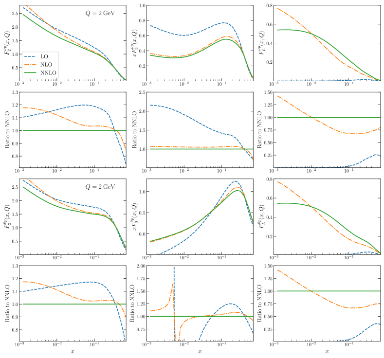
Figure 2.1: Comparison of YADISM-LO, YADISM-NLO, and YADISM-NNLO calculations of the $F_{2}^{\nu p}$, $xF_{3}^{\nu p}$, and $F_{L}^{\nu p}$ structure functions and their antineutrino counterparts as a function of $x$ for $Q=2$ GeV. The three calculations use the central set of NNPDF4.0 NNLO as input and do not display the PDF uncertainties. We show both the absolute structure functions and their ratios to the NNLO calculation.

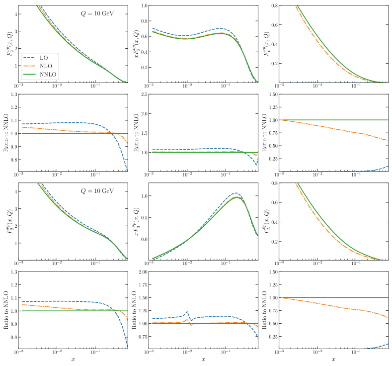
Figure 2.2: Same as Fig. 2.1 for $Q=10$ GeV.

It is found that for $Q=2$ GeV higher-order QCD corrections are in general significant and exhibit a similar pattern both for neutrinos and for antineutrinos. For the dominant $F_{2}$ structure function, the LO calculation underestimates at large-$x$ the NNLO result for up to 25%, while for $x\mathrel{\hbox to0.0pt{\lower 4.0pt\hbox{\hskip 1.0pt$\sim$}\hss}\raise 1.0pt\hbox{$<$}}0.2$ it overestimates it by more than 20%. NLO corrections reduce these differences at medium and large-$x$, but for $x\simeq 10^{-3}$ the NLO structure functions still overshoot the NNLO result by 20%. Since PDF uncertainties in $F_{2}$ are at the few percent level at most (see below), at $Q=2$ GeV missing higher order uncertainties (MHOU) are the main source of theory errors. Concerning the parity-violating structure function $xF_{3}$, for neutrino beams the LO calculation overestimates the NNLO result by 50% at $x=0.1$ and by a factor 2 for $x=10^{-2}$. A similar pattern is observed for antineutrinos, with now LO becoming more negative at small-$x$ while NLO is similar to NNLO. The longitudinal structure function $F_{L}$ vanishes at LO and displays large NNLO corrections, up to $+40\%$ as compared to the NLO result.

Once we increase the scale to $Q=10$ GeV, the perturbative expansion exhibits an improved convergence, and in particular differences between NLO and NNLO structure functions (for a fixed common PDF set) are moderate in all cases. The only exception is $F_{L}$ at large-$x$, a region anyway not relevant for phenomenology since $F_{2}$ is much larger there. Nevertheless, neglecting NLO and NNLO coefficients functions still leads to sizable differences, specially for $F_{2}$, of up to 10% at small-$x$ and $-20\%$ at large-$x$.

Benchmarking.

Fig. 2.3 compares the neutrino structure functions on a proton target in the YADISM-LO, Bodek-Yang, LO-SF-NNPDF4.0, and LO-SF-GRV98 calculations as a function of $x$ for $Q=2$ GeV and $Q=10$ GeV and then as a function of $Q$ (in the perturbative region) for $x=0.0126$ and $x=0.25$. In the case of LO-SF-NNPDF4.0, we show the 68% CL uncertainties, evaluated over $N_{\rm rep}=100$ Monte Carlo replicas.

As expected, YADISM-LO coincides with the central value of LO-SF-NNPDF4.0 for all values of $Q$. Residual differences are found only at large-$x$ and small-$Q$ and are explained in terms of the target mass corrections (TMCs) accounted for in the YADISM calculation. Likewise, Bodek-Yang reduces to LO-SF-GRV98 at large-$Q$, and in particular at $Q\simeq 10$ GeV the two calculations are almost identical. This agreement indicates that the phenomenological corrections to the GRV98 LO PDFs in the Bodek-Yang model have a negligible effect for $Q\mathrel{\hbox to0.0pt{\lower 4.0pt\hbox{\hskip 1.0pt$\sim$}\hss}\raise 1.0pt\hbox{$>$}}10$ GeV, while they become instead important at low-$Q$. For instance, at $Q=2$ GeV, the differences between Bodek-Yang and LO-SF-GRV98 range between 10% and 30% depending on the structure function and the value of $x$.

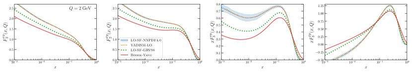
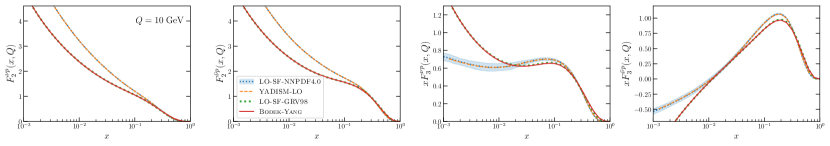
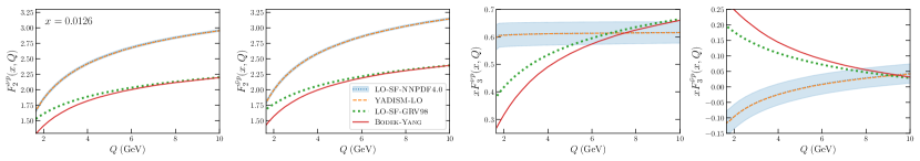
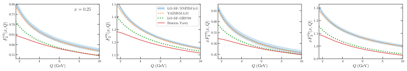
Figure 2.3: Neutrino structure functions on a proton target, comparing the YADISM-LO, Bodek-Yang, LO-SF-NNPDF4.0, and LO-SF-GRV98 predictions. We display, from top to bottom, $F_{2}^{\nu p}$, $F_{2}^{\bar{\nu}p}$, $xF_{3}^{\nu p}$, and $xF_{3}^{\bar{\nu}p}$ first as a function of $x$ for $Q=2$ GeV and $Q=10$ GeV and then as a function of $Q$ for $x=0.0126$ and $x=0.25$. For LO-SF-NNPDF4.0 we also show the 68% CL PDF uncertainties.

The comparisons of Fig. 2.3 also highlight the typical behaviours of the neutrino structure functions in different regions of the $(x,Q^{2})$ plane. Concerning the $x$ dependence, that of $F_{2}^{\nu p}$ and $F_{2}^{\bar{\nu}p}$ is similar and displays the valence peak at $x\simeq 0.3$ followed by the rise at small-$x$ driven by DGLAP evolution, which is more marked the higher the value of $Q$. In the case of $xF_{3}$, being a non-singlet structure function, the valence peak is followed by a small-$x$ behaviour that depends on the value of $Q$ and of whether the beam is composed by neutrinos or anti-neutrinos, since in each case the quark flavour combinations, Eq. (2.11), are different. In terms of the $Q$ dependence, whether higher $Q$ values lead to an increase or a decrease of the structure function depends on the value of $x$. For $F_{2}^{\nu p}$ and $F_{2}^{\bar{\nu}p}$ the structure functions grow (decrease) with $Q$ for $x=0.0126$ ($x=0.25$). For $xF_{3}$ also for $x=0.25$ there is a similar decrease with $Q$, while for $x=0.0126$ the $Q$ dependence varies strongly with the choice of input PDF set.

Given that in Fig. 2.3 all calculations shown are based on LO coefficient functions, the significant differences between Bodek-Yang and YADISM-LO as $Q$ is increased can only be attributed to those at the input PDFs level, GRV98LO and NNPDF4.0 NNLO respectively. For instance, for $F_{2}^{\nu p}$ the GRV98LO calculation undershoots the YADISM-LO one based on NNPDF4.0 by 40% at $x\simeq 10^{-2}$ and $Q=10$ GeV and by 10% at $x=0.25$ and $Q=6$ GeV. In the case of $xF_{3}$, the small-$x$ behaviour is qualitatively different between GRV98 and NNPDF4.0, for example at $Q=10$ GeV for $xF_{3}^{\nu p}$ the former predicts a steep rise while a flat extrapolation is preferred by the latter. This indicates that predictions based on the Bodek-Yang model, and thus on the obsolete GRV98LO PDF set, will in general disagree with those based on modern PDF determinations.

PDF dependence.

We compare in Fig. 2.4 the YADISM-NLO predictions with those from the Bodek-Yang and BGR18 calculations. The YADISM-NLO and BGR18 predictions are very similar, consistent with the agreement within uncertainties of the underlying NNPDF4.0 and NNPDF3.1 PDF fits respectively. Differences between YADISM-NNLO and Bodek-Yang are significant, specially for $F_{2}$ in the $x\mathrel{\hbox to0.0pt{\lower 4.0pt\hbox{\hskip 1.0pt$\sim$}\hss}\raise 1.0pt\hbox{$<$}}0.1$ region and for $xF_{3}$ at small-$x$. These differences are explained by the reliance of BY on the obsolete GRV98LO PDF set (cfr Fig. 2.3) and due to neglecting higher-order QCD corrections (cfr Figs. 2.1 and 2.2).

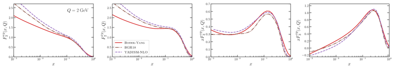
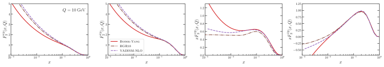
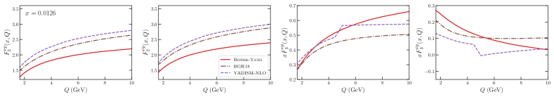
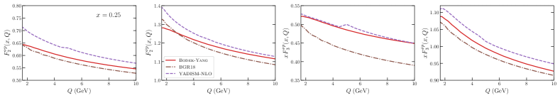
Figure 2.4: Same as Fig. 2.3 comparing the Bodek-Yang, BGR18, and YADISM-NLO structure functions.

The longitudinal structure function.

In Fig. 2.3 we display the $F_{2}$ and $xF_{3}$ structure functions which provide the dominant contribution to the double-differential cross section Eq. (2.5). While the longitudinal structure function $F_{L}$ vanishes at LO, it becomes non-zero at NLO and in specific kinematic regions can lead to non-negligible contributions to the scattering cross sections. To illustrate this hierarchy in the relative magnitude of the different structure functions, Fig. 2.5 displays their ratio to $F_{2}$ for neutrinos and antineutrinos for $Q=2$ GeV and $Q=10$ GeV in the YADISM-NNLO calculation.

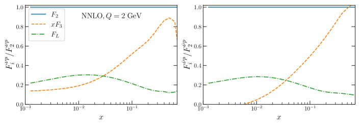
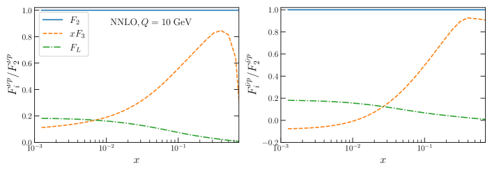
Figure 2.5: The ratio of the neutrino structure functions to $F_{2}$ for neutrinos (left) and antineutrinos (right) for $Q=2$ GeV (top) and $Q=10$ GeV (bottom panels) in YADISM-NNLO.

From Fig. 2.5 we observe how in the large-$x$ valence region the $F_{2}$ and $xF_{3}$ structure functions are of comparable magnitude, with $F_{L}$ being much smaller. Since $xF_{3}$ is a valence structure function, it is suppressed as $x$ decreases and indeed for $x=10^{-2}$ it becomes at most 20% of the value of the dominant $F_{2}$. The relative contribution from $F_{L}$ is similar for neutrinos and neutrinos, since it is dominated by the gluon contribution, and becomes more important as both $x$ and $Q^{2}$ decrease. In particular, for $x\mathrel{\hbox to0.0pt{\lower 4.0pt\hbox{\hskip 1.0pt$\sim$}\hss}\raise 1.0pt\hbox{$<$}}10^{-2}$ the magnitude of $F_{L}$ becomes larger than that of $xF_{3}$. At $Q=2$ GeV, $F_{L}$ can be up to 30% the value of $F_{2}$, indicating a contribution to the double differential cross section larger than the typical experimental uncertainties and that hence must be accounted for.

Whenever possible, we fit data for the double-differential cross section rather than for the individual $F_{2}$ and $xF_{3}$ structure functions separately, since the former provides also sensitivity to $F_{L}$.

3 The NNSF$\nu$ approach

Here we describe the NNSF$\nu$ approach used to determine neutrino-nucleon inelastic structure functions and their associated uncertainties across the whole range of $Q$ relevant for neutrino phenomenology. We first describe the general strategy, based on the combination of a machine-learning parametrisation of experimental data with state-of-the-art QCD calculations. We then review the available measurements on neutrino structure functions and cross sections used to constrain this parametrisation. Subsequently, we discuss the neural network parametrisation of neutrino structure functions, how it is trained on both the data and the QCD predictions, and the uncertainty estimate based on the Monte Carlo replica method.

3.1 General strategy

An schematic representation of the NNSF$\nu$ strategy to determine neutrino structure functions is displayed in Fig. 3.1 with the Bodek-Yang predictions at $x=0.0126$ for illustration. The $(x,Q)$ plane is divided into three disjoint regions, with complementary methods to evaluate the structure functions in each of them:

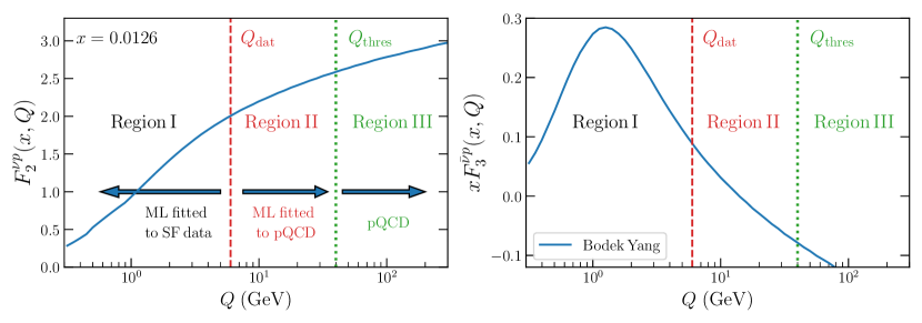
Figure 3.1: Schematic representation of the NNSF$\nu$ strategy. In the region with $Q\leq Q_{\rm dat}$ (Region I), we adopt a data-driven approach where a neural network parametrisation is fitted to neutrino inelastic structure function data. In the intermediate region with $Q_{\rm dat}\leq Q\leq Q_{\rm thr}$ (Region II), the same parametrisation is fitted instead to the QCD calculations provided by YADISM with nNNPDF3.0 as input. In the high-$Q$ region, $Q>Q_{\rm thr}$ (Region III), the neural network predictions are replaced by the outcome of the same YADISM calculation. For small-$x$ values relevant for UHE neutrino scattering ($x\leq 10^{-5}$), Region III is extended to cover $Q_{\rm min}\leq Q\leq Q_{\rm thr}$ with $Q_{\rm min}=2$ GeV, see App. A for more details and Fig. A.1 in particular for the analogous division into regions at the level of the $(x,Q^{2})$ plane.

• Region I. At low momentum transfers $Q\mathrel{\hbox to0.0pt{\lower 4.0pt\hbox{\hskip 1.0pt$\sim$}\hss}\raise 1.0pt\hbox{$<$}}Q_{\rm dat}$, with $Q_{\rm dat}\simeq 5$ GeV, the perturbative calculation of neutrino structure functions in Eq. (2.9) is either invalid or affected by significant theory uncertainties related to higher twists, missing higher perturbative orders, and large-$x$ resummation effects.

  In this region we parametrise the structure functions in terms of the information provided by the available experimental data on neutrino-nucleus inelastic scattering summarised in Sect. 3.2. Following the NNPDF fitting methodology, this parametrisation combines neural networks as universal unbiased interpolants with the Monte Carlo replica method for the uncertainty estimate.

• Region II. The region of intermediate momentum transfers, $Q_{\rm dat}\mathrel{\hbox to0.0pt{\lower 4.0pt\hbox{\hskip 1.0pt$\sim$}\hss}\raise 1.0pt\hbox{$<$}}Q\mathrel{\hbox to0.0pt{\lower 4.0pt\hbox{\hskip 1.0pt$\sim$}\hss}\raise 1.0pt\hbox{$<$}}Q_{\rm thr}$ with $Q_{\rm thr}\simeq 25$ GeV, is well described by the perturbative QCD formalism. DIS structure functions are computed at NLO by YADISM with nNNPDF3.0 as input for all targets. In this region the neural network parametrisation is fitted to these QCD predictions rather than to the data as in Region I. The figure of merit is given in terms of the theory covariance matrix with PDF and the MHO uncertainties, see Sect. 3.4.

  The nNNPDF3.0 determination already includes information from neutrino measurements, in particular from CHORUS (inclusive) and NuTeV (charm) structure functions, and therefore in Region II no neutrino data needs to be explicitely used to further constrain the parametrisation.

• Region III. For large momentum transfers, $Q\mathrel{\hbox to0.0pt{\lower 4.0pt\hbox{\hskip 1.0pt$\sim$}\hss}\raise 1.0pt\hbox{$>$}}Q_{\rm thr}$, the neural network predictions are replaced by the direct outcome of the same YADISM calculation used to constrain the fit in Region II. Hence, in Region III the central prediction and uncertainties of NNSF$\nu$ coincide with the YADISM ones, which extend up to $Q=10$ TeV and down to $x=10^{-9}$ to cover the entire kinematic region relevant for neutrino phenomenology including the UHE scattering.

  Furthermore, Region III is extended in the small-$x$ region with $x\leq 10^{-5}$ to cover also momentum transfers of $Q_{\rm min}\leq Q\leq Q_{\rm thr}$, with $Q_{\rm min}=2$ GeV. The reason for this choice is that for $x\leq 10^{-5}$ the neural network extrapolation trained in Regions I and II exhibits large uncertainties and using the QCD calculation is preferred on theoretical grounds [73].

As we will show in the subsequent sections, such a strategy allows us to consistently extend the state-of-the-art perturbative QCD computations into the non-perturbative region and provide predictions that are valid across a wide range of energy relevant for neutrino phenomenology.

We have verified that the NNSF$\nu$ determination is stable with respect to moderate variations of the values of the $Q_{\rm dat}$ and $Q_{\rm thr}$ hyperparameters. App. A provides additional details on the implementation of the NNSF$\nu$ procedure including the prescriptions to evaluate and match inelastic structure functions in the various regions of the $(x,Q^{2})$ kinematic plane.

3.2 Experimental data

The parametrisation of neutrino structure functions applicable in Regions I and II defined in Fig. 3.1 requires two different inputs: experimental data in Region I and the corresponding QCD calculations for Region II. For the former, we consider all available data on inelastic neutrino structure functions and double differential cross sections. We restrict our analysis to those measurements where the incoming neutrino energy $E_{\nu}$ is sufficiently large to ensure that the contribution from the inelastic region dominates. For this reason, we do not consider neutrino measurements from experiments such as ArgoNeuT [74], MicroBooNE [75], T2K [76], or MINER$\nu$A [77], where $E_{\nu}$ is too low to cleanly access inelastic scattering.

Two kinematic cuts are applied to the data used as input to the NNSF$\nu$ fit. First, a cut in the invariant mass of the final hadronic state $W^{2}\geq 3.5\leavevmode\nobreak\ \rm{GeV}^{2}$ filters away points in the quasi-elastic and resonant scattering regions. Second, data points with $Q\geq Q_{\rm dat}$ are excluded according to the definition of Region I in Fig. 3.1. This cut does not result on a net information loss in the fit, since as mentioned above nNNPDF3.0 already includes the constraints from neutrino DIS data present in the $Q\geq Q_{\rm dat}$ region.

Table 3.1 lists the datasets used to constrain neutrino structure functions in Region I. For each dataset, we indicate the publication reference, the range of $x$ and $Q^{2}$ covered, the observables included, the scattering target, the final state measured, and the number of available data points $n_{\rm dat}$ before and after applying kinematic cuts. In total we have 6224 (4184) data points in the fit before (after) cuts. The corresponding kinematic coverage of these datasets in the $(x,Q^{2})$ plane is displayed in Fig. 3.2, which also indicates the regions excluded by cuts. Some of the datasets from Table 3.1 provide additional observables on top of those indicated there, which however need to be excluded from the fit to prevent double counting. In particular, the same measurement is often presented in terms of both the differential cross section $d^{2}\sigma/dxdQ^{2}$ and of the individual structure functions $F_{2}$ and $xF_{3}$. We always select observables that are closer to the actual measurements, in this case the double differential cross-sections as they also constrain the longitudinal structure function $F_{L}$.

Dataset	Ref.	$\left[x_{\text{min}},\leavevmode\nobreak\ x_{\text{max}}\right]$	$\left[Q_{\text{min}}^{2},Q^{2}_{\text{max}}\right]\leavevmode\nobreak\ (\rm{GeV}^{2})$	Observables	Target	Final state	$n_{\rm dat}\,\left(n_{\rm dat}^{(\rm fit)}\right)$
BEBCWA59	[78]	$[0.028,0.65]$	$[0.2,44]$	$F_{2},xF_{3}$	Ne	$\nu+\bar{\nu}$	114 (71)
CCFR	[79]	$[0.015,0.65]$	$[1.3,126]$	$F_{2},xF_{3}$	Fe	$\nu+\bar{\nu}$	256 (164)
CHARM	[80]	$[0.015,0.80]$	$[0.2,78]$	$F_{2},xF_{3}$	CaCO3	$\nu+\bar{\nu}$	320 (144)
CHORUS	[81]	$[0.020,0.65]$	$[0.3,101]$	$d^{2}\sigma/dxdQ^{2}$	Pb	$\nu$, $\bar{\nu}$	1212 (966)
CDHSW	[82]	$[0.015,0.65]$	$[0.2,196]$	$d^{2}\sigma/dxdQ^{2}$	Fe	$\nu$, $\bar{\nu}$	1551 (1259)
NuTeV	[83]	$[0.015,0.75]$	$[1.1,279]$	$d^{2}\sigma/dxdQ^{2}$	Fe	$\nu$, $\bar{\nu}$	2874 (1580)
Total							6224 (4184)

Table 3.1: Datasets included in the NNSF$\nu$ fit for Region I of Fig. 3.1. We indicate the publication reference, the range of $x$ and $Q^{2}$, the observables included, the scattering target, the final state measured, and the number of data points before (after) applying kinematic cuts. The coverage of these datasets in the $(x,Q^{2})$ plane is displayed in Fig. 3.2. Some of experiments provide additional observables, which are excluded to prevent double counting.

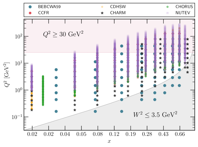
Figure 3.2: The kinematic coverage in the $(x,Q^{2})$ plane of the neutrino scattering cross-section data listed in Table 3.1. The region covered in grey is excluded from the fit from $W^{2}\geq 3.5\leavevmode\nobreak\ \rm{GeV}^{2}$ cut required to isolate inelastic scattering, while the one in light red is excluded from the $Q\leq Q_{\rm dat}$ condition that defines Region I in Fig. 3.1.

Table 3.1 and Fig. 3.2 indicate that the NNSF$\nu$ fit is sensitive to inelastic neutrino structure functions for momentum transfers down to $Q\simeq 400$ MeV, well in the non-perturbative region. The range of $x$ covered reaches $x_{\rm min}=0.015$, and as a consequence of the DIS kinematics the values of $Q$ being probed increase with $x$. Measurements in the non-perturbative region with $Q\mathrel{\hbox to0.0pt{\lower 4.0pt\hbox{\hskip 1.0pt$\sim$}\hss}\raise 1.0pt\hbox{$<$}}1$ GeV are provided by several experiments and cover momentum fractions up to $x\mathrel{\hbox to0.0pt{\lower 4.0pt\hbox{\hskip 1.0pt$\sim$}\hss}\raise 1.0pt\hbox{$<$}}0.3$. The datasets with the largest number of points (CHORUS, NuTeV, and CDHSW) present their measurements in terms of the double differential cross section $d^{2}\sigma/dxdy$, while BEBCWA59, CCFR, and CHARM only provide data for separate structure functions $F_{2}$ and $xF_{3}$.

Concerning nuclear effects, Table 3.1 shows that available data have sensitivity to neutrino scattering on Ne ($A=20$), Fe $(A=56)$, and Pb ($A=208$) targets. For CaCO3, the target used in the CHARM experiment, we assume $A=20$ as the average atomic mass number of the nuclei that form this compound. Neutrino structure function measurements are not available on hydrogen or deuteron targets, and hence in Region I the low-$A$ behaviour is extrapolated from the measurements with $A\geq 20$. The inter- and extrapolation to $A$ values not included in the fit is provided by the smoothness of the neural network output, as we validate in Sect. 4.

For momentum transfers $Q>Q_{\rm dat}$ (Regions II and III) the dependence with the atomic mass number $A$ of NNSF$\nu$ follows that provided by nNNPDF3.0, and is hence constrained by other types of processes beyond neutrino DIS, such as charged-lepton fixed-target nuclear DIS and weak boson, dijet, and $D$-meson production cross sections in proton-lead collisions at the LHC.

3.3 Structure function parametrisation

The NNSF$\nu$ parametrisation of neutrino structure functions in Regions I and II is obtained by training a machine learning model to experimental data and to the QCD predictions, respectively. It follows the NNPDF fitting methodology based on the combination of neural networks as universal unbiased interpolator with the Monte Carlo replica method for error estimate and propagation. This methodology was originally developed for DIS neutral-current structure functions [63, 62] and subsequently extended to proton PDFs [54, 56, 84, 59, 61, 60], helicity PDFs [85, 86], nuclear PDFs [87, 72, 65], and fragmentation functions [88, 89].

Here we apply for the first time the NNPDF approach to i) the determination of neutrino (charged-current) structure functions and to ii) the parametrisation of a three-dimensional function, with neural networks receiving $(x,Q^{2},A)$ as inputs. This is achieved by means of a stand-alone open-source NNSF$\nu$ framework described in App. A. This framework shares many similarities with the NNPDF4.0 codebase, in particular it is also built upon TensorFlow [90] and uses adaptative stochastic gradient descent (SGD) methods for the minimisation such as Adam [91].

The double-differential neutrino-nucleus cross sections, Eqns. (2.1) and (2.3), are expressed in terms of three independent structure functions and hence one needs to parametrise six independent quantities which we choose to be

$$F_{2}^{\nu}(x,Q^{2},A)\,,\quad xF_{3}^{\nu}(x,Q^{2},A)\,,\quad F_{L}^{\nu}(x,Q^{2},A)\,,$$

$$F_{2}^{\bar{\nu}}(x,Q^{2},A)\,,\quad xF_{3}^{\bar{\nu}}(x,Q^{2},A)\,,\quad F_{L}^{\bar{\nu}}(x,Q^{2},A)\,,\quad$$ (3.1)

each of them function of the three inputs $(x,Q^{2},A)$. In Eq. (3.1) the limit $A=1$ is to be understood as that of the structure functions on an isoscalar, free-nucleon target, rather than those for a proton target. That is, $F_{2}^{\nu}(x,Q^{2},A=1)$ coincides with $\left(F_{2}^{\nu p}(x,Q^{2})+F_{2}^{\nu n}(x,Q^{2})\right)/2$, and likewise for the other structure functions.

The mapping between the inputs $(x,Q^{2},A)$ and the outputs $F_{i}^{\nu},F_{i}^{\bar{\nu}}$ with $i=2,3,L$ in Eq. (3.1) is provided by a deep neural network as illustrated in Fig. 3.3. The free parameters of this neural network, its weights and thresholds, are determined by training the parametrisation to the experimental data (in Region I) and to the QCD predictions (in Region II) for neutrino structure functions and differential cross sections. Hyperparameters like the network architecture are determined by means of a dedicated optimisation procedure. The best choice for the architecture of this network is found to be 3–70–55–40–20–20–6, hence composed by five hidden layers with 70, 55, 40, 20, and 20 neurons in each of them.

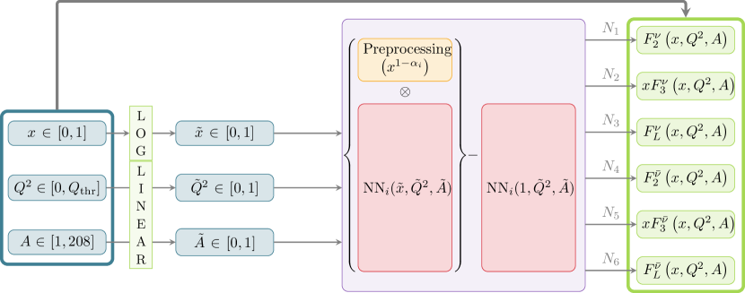
Figure 3.3: Flowchart summarizing the NNSF$\nu$ fitting framework. The three inputs are the momentum fraction $x$, the momentum transfer squared $Q^{2}$, and the atomic mass number $A$, suitably preprocessed to lie in a common range. The network output is supplemented by a power-like term to facilitate the learning of the small-$x$ region and the endpoint behaviour at $x=1$ is subtracted to reproduce the elastic limit. The architecture of this neural network is 3-70-55-40-20-20-6 and hence composed by five hidden layers. The parameters of the neural network are optimised to reproduce the experimental data in Region I and the QCD predictions in Region II.

As indicated by Fig. 3.3, two corrections are applied to the network output before it can be identified with the neutrino structure functions. First, we supplement the network output with a preprocessing factor $x^{1-\alpha_{i}}$ that facilitates the learning and extrapolation of structure functions in the small-$x$ region [73]. Second, we subtract the endpoint behaviour at $x=1$ to reproduce the elastic limit where structure functions vanish due to kinematic constraints. With these considerations, the relation between the network output and the structure functions is given by

$$F_{i}^{\nu}(x,Q^{2},A) = x^{1-\alpha_{i}}{\rm NN}_{i}(x,Q^{2},A)-{\rm NN}_{i}(x=1,Q^{2},A)\,,$$ (3.2)

$$F_{i}^{\bar{\nu}}(x,Q^{2},A) = x^{1-\bar{\alpha}_{i}}{\rm NN}_{3+i}(x,Q^{2},A)-{\rm NN}_{3+i}(x=1,Q^{2},A)\,,$$

for $i=1,2,3$ corresponding to $F_{2},xF_{3},F_{L}$, and where ${\rm NN}_{j}$ indicates the activation state of the $j$-th neuron in the output layer of the network.

By construction, structure functions parametrised this way vanish in the elastic limit $x=1$ for all values of $Q^{2}$ and $A$ without restricting the behaviour in the $x<1$ region. The small-$x$ preprocessing exponents $\left(\alpha_{i},\alpha_{i}\right)$ in Eq. (3.2) are constrained from the data as part of the training procedure at the same time as the neural network parameters. Furthermore, the neural network inputs are rescaled to a common range, logarithmically in $x$ and linearly in $Q^{2}$ and $A$ to ensure that no specific kinematic region is arbitrarily privileged by the training. We do not enforce the positivity of the $F_{2}$ and $F_{L}$ structure functions, since it is found that the data together with the QCD constraints included are sufficient to avoid the unphysical negative region.

3.4 Fitting and error propagation

The neural network parametrisation of neutrino structure functions from Fig. 3.3 is constrained by the experimental data from Table 3.1 in Region I and by the QCD predictions in Region II. Here we discuss the figures of merit used in the minimisation, the error propagation strategy based on the Monte Carlo replica method, and the settings and performance of the training procedure.

Fig. 3.4 provides a diagrammatic representation illustrating the evaluation of the figure of merit in the fit, $\chi^{2}$, as a function of the kinematic inputs ${\bm{z}}_{i}=\left\{x_{i},Q^{2}_{i},A_{i}\right\}$ with $i$ labelling the fitted data points. The structure functions parametrised by neural networks according to Eq. (3.2) and Fig. 3.3 are combined to construct the observables that input the fit e.g. by means of Eqns. (2.5) and (2.6). These fit inputs are classified into experimental data and QCD calculations depending on the range of $Q^{2}$ being considered. The predicted observables from the neural network parametrisation are then compared to the corresponding input data points to evaluate the $\chi^{2}$ entering both the optimisation process and the cross-validation stopping.

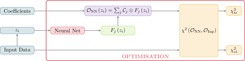
Figure 3.4: Diagrammatic representation of the evaluation of the figure of merit in the fit, $\chi^{2}$, as a function of the kinematic inputs ${\bm{z}}_{i}=\left\{x_{i},Q^{2}_{i},A_{i}\right\}$ with $i=1,\ldots,n_{\rm dat}^{(\rm fit)}$. The structure functions parametrised by neural networks according to Eq. (3.2) and Fig. 3.3 are combined to construct the observables that input $(\mathcal{O}_{\rm Inp})$ the fit (and composed by either experimental data or QCD calculations) e.g. by means of Eqns. (2.5) and (2.6). The predicted observables are compared to the corresponding data points to evaluate the $\chi^{2}$ entering the optimisation process and the cross-validation stopping. $\chi^{2}_{\rm tr}$ and $\chi^{2}_{\rm vl}$ represent the training and validation losses, respectively.

Constraints from experimental data.

In the Monte Carlo replica method one first generates a sample of $N_{\rm rep}$ artificial replicas of the experimental data as follows. Given $n_{\rm dat}$ experimental measurements of neutrino structure functions or differential cross sections characterised by central value $\mathcal{F}^{{\rm(dat)}}_{i}$, uncorrelated uncertainty $\sigma_{i}^{\rm(stat)}$, $n_{\rm sys}$ correlated systematic uncertainties $\sigma^{\rm(sys)}_{i,\alpha}$, and $n_{\rm norm}$ normalisation uncertainties $\sigma^{\rm(norm)}_{i,n}$, artificial replicas of these measurements are generated by

$$\mathcal{F}_{i}^{(\mathrm{art})(k)}=\left[\prod_{n=1}^{n_{\rm norm}}\left(1+r_{i,n}^{(k)}\sigma^{\rm(norm)}_{i,n}\right)\right]\mathcal{F}_{i}^{\rm(dat)}\left(1+r_{i}^{(k)}\sigma_{n}^{\rm(stat)}+\sum_{\alpha=1}^{n_{\rm sys}}r_{i,\alpha}^{(k)}\sigma^{\rm(sys)}_{i,\alpha}\right)\ ,\quad k=1,\ldots,N_{\mathrm{rep}}\,,$$ (3.3)

for $i=1,\ldots,n_{\rm dat}$, where $r_{i}^{(k)}$, $r_{i,\alpha}^{(k)}$, and $r_{i,n}^{(k)}$ indicate univariate Gaussian random numbers generated such that experimental correlations between systematic and normalisation errors are accounted for. This procedure is formally equivalent to generating data replicas according to the statistical model provided by the experimental covariance matrix, which is reproduced by averaging over replicas,

$$\left\langle\mathcal{F}_{i}^{(\mathrm{art})}\mathcal{F}_{j}^{(\mathrm{art})}\right\rangle_{\rm rep}-\left\langle\mathcal{F}_{i}^{(\mathrm{art})}\right\rangle_{\mathrm{rep}}\left\langle\mathcal{F}_{j}^{(\mathrm{art})}\right\rangle_{\rm rep}=\qquad\qquad\qquad\qquad$$ (3.4)

$${{1}\over{N_{\rm rep}}}\sum_{k=1}^{N_{\rm rep}}\mathcal{F}^{{(\rm art)}(k)}_{i}\mathcal{F}^{{(\rm art)}(k)}_{j}-{{1}\over{N_{\rm rep}^{2}}}\sum_{k=1}^{N_{\rm rep}}\mathcal{F}^{{\rm{(art)}}(k)}_{i}\sum_{k^{\prime}=1}^{N_{\rm rep}}\mathcal{F}^{{\rm{(art)}}(k^{\prime})}_{j}=\left({\rm cov}_{\rm exp}\right)_{ij}\,,$$

in the large replica limit, $N_{\rm rep}\to\infty$. For the neutrino structure function data considered in NNSF$\nu$, ${\rm cov}_{\rm exp}$ contains only additive systematic uncertainties and hence it is not affected by the D’Agostini bias which would require introducing a $t_{0}$ covariance matrix [92] based on a previous iteration of the fit.

Subsequently, for each of the $N_{\rm rep}$ replicas generated according to Eq. (3.3), a separate neural network with the structure of Fig. 3.3 is trained by minimising the error function defined as

$$E_{\rm exp}^{(k)}={{1}\over{n_{\rm dat}}}\sum_{i,j=1}^{n_{\mathrm{dat}}}\left(\mathcal{F}^{{\rm(net)}(k)}_{i}-\mathcal{F}^{{\rm(art)}(k)}_{i}\right)\left(\operatorname{cov}_{\rm exp}^{-1}\right)_{ij}\left(\mathcal{F}^{{\rm(net)}(k)}_{j}-\mathcal{F}^{{\rm(art)}(k)}_{j}\right)\,,\quad k=1,\ldots,N_{\mathrm{rep}}\ ,$$ (3.5)

in terms of the experimental covariance matrix. For each replica, the training is stopped once the cross-validation stopping criterion described below is satisfied. The overall goodness-of-fit between the model predictions and the experimental data is then quantified by the $\chi^{2}$ defined in a similar manner as Eq. (3.5) now in terms of the average neural network prediction,

$$\chi^{2}_{\rm exp}={{1}\over{n_{\rm dat}}}\sum_{i,j=1}^{n_{\mathrm{dat}}}\left(\left\langle\mathcal{F}^{\rm(net)}_{i}\right\rangle_{\rm rep}-\mathcal{F}^{\rm(dat)}_{i}\right)\left(\operatorname{cov}_{\rm exp}^{-1}\right)_{ij}\left(\left\langle\mathcal{F}^{\rm(net)}_{j}\right\rangle_{\rm rep}-\mathcal{F}^{\rm(dat)}_{j}\right)\,,$$ (3.6)

with averages over replica sample are evaluated as

$$\left\langle\mathcal{F}^{\rm(net)}_{i}\right\rangle_{\rm rep}={{1}\over{N_{\rm rep}}}\sum_{k=1}^{N_{\rm rep}}\mathcal{F}^{{{\rm(net)}}(k)}_{i}\,.$$ (3.7)

The $N_{\rm rep}$ trained neutral network parametrisations provide a representation of the probability density in the space of neutrino structure functions, from which expectation values and other statistical estimators can be computed. For instance, the $1\sigma$ uncertainty $\delta\mathcal{F}$ in a structure function at generic $(x,Q^{2},A)$ values can be computed by evaluating the standard deviation over the replica ensemble,

$$\delta\mathcal{F}(x,Q^{2},A)=\left[{{1}\over{N_{\rm rep}}}\sum_{k=1}^{N_{\rm rep}}\left(\mathcal{F}^{{\rm{(net)}}(k)}(x,Q^{2},A)\right)^{2}-\left(\left\langle\mathcal{F}^{\rm(net)}(x,Q^{2},A)\right\rangle_{\rm rep}\right)^{2}\right]^{1/2}\,,$$ (3.8)

where $\mathcal{F}$ represents any of the three structure functions $F_{2},xF_{3}$, and $F_{L}$. Similar considerations apply to other statistical estimators such as correlations coefficients, higher moments, and confidence level intervals.

Both the experimental covariance matrix and the associated correlation matrix given by

$$\left(\rho_{\mathrm{exp}}\right)_{ij}={{\left(\operatorname{cov}_{\rm exp}\right)_{ij}}\over{\sqrt{\left(\operatorname{cov}_{\rm exp}\right)_{ii}}\sqrt{\left(\operatorname{cov}_{\rm exp}\right)_{jj}}}}\,,$$ (3.9)

are displayed in the left panels of Fig. 3.5 for the data points listed in Table 3.1 after cuts. The matrices are block-diagonal since the different experiments are uncorrelated among them. In most cases, neutrino inelastic scattering experiments are limited by the correlated systematic uncertainties rather than by the statistical errors.

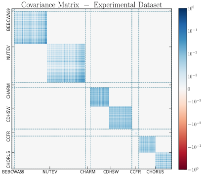
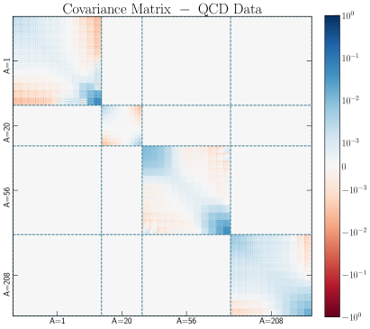
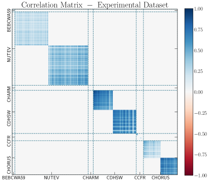
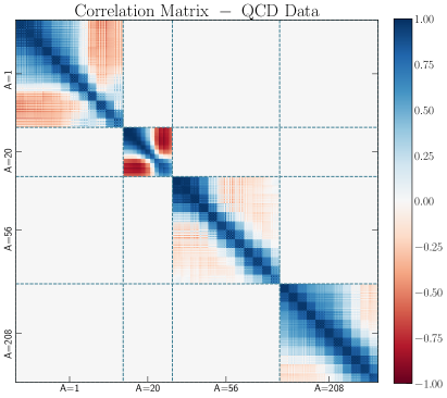
Figure 3.5: Left panels: the experimental covariance (top) and correlation (bottom) matrices relevant for the fit in Region I. Right panels: same for the theory covariance matrix associated to the QCD data entering the fit in Region II, with data points ordered in increasing order of $x$, $Q^{2}$, and $A$. There is no kinematic overlap between the entries of the experimental and theoretical matrices.

QCD constraints.

In Region II, the same neural network parameterisation is trained now on QCD predictions based on YADISM and nNNPDF3.0 rather than to the experimental data. Taking the central nNNPDF3.0 set as baseline, we generate $n_{\rm th}=100\times n_{\rm sf}$ structure function QCD predictions distributed in $x$, $Q^{2}$, and $A$ covering Region II,

$$10^{-3}\leq x\leq 1\,,\qquad Q^{2}_{\rm dat}\leq Q^{2}\leq Q^{2}_{\rm thr}\,,\qquad 1\leq A\leq 208\,,$$ (3.10)

with $n_{\rm sf}=6$ denoting the number of independent structure functions being parametrised. As indicated in Eq. (3.10) we include a QCD boundary condition for $A=1$, understood as an isoscalar free-nucleon target.

By analogy with Eq. (3.3), also in Region II one generates $N_{\rm rep}$ (independent) Monte Carlo replicas, this time starting from the central QCD predictions rather than from the experimental data. If we denote these central QCD structure functions by $\mathcal{F}_{i}^{(\rm qcd)(0)}$, we generate $N_{\rm rep}$ replicas as follows

$$\mathcal{F}^{\rm(qcd)}_{i} = \mathcal{F}^{\rm(qcd)(0)}_{i}+\sum_{j=1}^{n_{\rm th}}\left(\operatorname{cov}_{\rm th}^{\star}\right)_{ij}r_{j}^{{(\rm th)}}\,,\quad i=1,\ldots,n_{\rm th}\,,$$

$$\mathcal{F}^{{\rm(qcd)}(k)}_{i} = \mathcal{F}^{\rm(qcd)}_{i}+\sum_{j=1}^{n_{\rm th}}\left(\operatorname{cov}_{\rm th}^{\star}\right)_{ij}r_{j}^{{(\rm th})(k)}\,,\quad k=1,\ldots,N_{\rm rep}\,,\quad i=1,\ldots,n_{\rm th}\,,$$ (3.11)

where $\operatorname{cov}_{\rm th}^{\star}$ indicates the transpose of the Cholesky decomposition of the theory covariance matrix and $r_{j}^{{(\rm th})}$, $r_{j}^{{(\rm th})(k)}$ represent stochastic noise sampled from a standard normal distribution. In order to treat the QCD data on the same footing as the experimental data, it is necessary to add two levels of stochastic noise to the central predictions $\mathcal{F}_{i}^{(\rm qcd)(0)}$: first to account the statistical fluctuations around the true underlying law, and second to generate the Monte Carlo replicas themselves. In the language of the closure test formalism [59], the first and second lines of Eq. (3.4) correspond to level-1 and level-2 pseudodata generation, while $\mathcal{F}_{i}^{(\rm qcd)(0)}$ is the level-0 underlying law.

The theory covariance matrix entering Eq. (3.4) is constructed [93, 94] as the sum in quadrature of the contributions from the MHO and PDF uncertainties,

$$\left(\operatorname{cov}_{\rm th}\right)_{ij}=\left(\operatorname{cov}_{\rm mho}\right)_{ij}+\left(\operatorname{cov}_{\rm pdf}\right)_{ij}\,,$$ (3.12)

where the MHOU contribution is evaluated using the NLO scheme-B with the 9-point scale variation prescription as implemented in YADISM, and the PDF contribution is evaluated from the $\widetilde{N}_{\rm rep}=200$ replicas of the nNNPDF3.0 determination. In constructing the theory covariance matrix Eq. (3.12), the correlations between different nuclear targets are neglected.

In Region II the figure of merit used for the neural network training should be, instead of Eq. (3.13),

$$E_{\rm th}^{(k)}={{1}\over{n_{\rm th}}}\sum_{i,j=1}^{n_{\mathrm{th}}}\left(\mathcal{F}^{{\rm(net)}(k)}_{i}-\mathcal{F}^{{\rm(qcd)}(k)}_{i}\right)\left(\operatorname{cov}_{\rm th}^{-1}\right)_{ij}\left(\mathcal{F}^{{\rm(net)}(k)}_{j}-\mathcal{F}^{{\rm(qcd)}(k)}_{j}\right)\,,\quad k=1,\ldots,N_{\mathrm{rep}}\ ,$$ (3.13)

with goodness-of-fit after the training of all replicas quantified now by the counterpart of Eq. (3.6),

$$\chi^{2}_{\rm th}={{1}\over{n_{\rm th}}}\sum_{i,j=1}^{n_{\mathrm{th}}}\left(\left\langle\mathcal{F}^{\rm(net)}_{i}\right\rangle_{\rm rep}-\mathcal{F}^{\rm(qcd)}_{i}\right)\left(\operatorname{cov}_{\rm th}^{-1}\right)_{ij}\left(\left\langle\mathcal{F}^{\rm(net)}_{j}\right\rangle_{\rm rep}-\mathcal{F}^{\rm(qcd)}_{j}\right)\,.$$ (3.14)

Analogously to the experimental case, we can define the theoretical correlation matrix as

$$\rho^{(\rm th)}_{ij}={{\left(\operatorname{cov}_{\rm th}\right)_{ij}}\over{\sqrt{\left(\operatorname{cov}_{\rm th}\right)_{ii}}\sqrt{\left(\operatorname{cov}_{\rm th}\right)_{jj}}}}$$ (3.15)

which is displayed, together with the corresponding theory covariance matrix, in the right panels of Fig. 3.5, where QCD data points are sorted in increasing order of $x$, $Q^{2}$, and $A$. Recall that there is no kinematic overlap between the entries of the experimental (Region I) and the theoretical (Region II) correlation matrices. One difference between $\rho^{(\rm th)}$ and $\rho^{(\rm exp)}$ is that in the former case QCD induces correlations between all data points (for a given value of $A$), arising because the same underlying nPDF determination is used as well as due to the correlation of factorisation scale variations entering DGLAP evolution.

Minimisation.

Adding up the contributions from the experimental data in Region I and from the QCD predictions in Region II, the total figure of merit used for the training of the neural network parametrisation of neutrino structure functions is given by

$$E_{\rm tot}^{(k)}={{1}\over{\left(n_{\rm dat}+n_{\rm th}\right)}}\left(n_{\rm dat}E_{\rm exp}^{(k)}+n_{\rm th}E_{\rm th}^{(k)}\right)\,,\quad k=1,\ldots,N_{\mathrm{rep}}\,.$$ (3.16)

In minimising Eq. (3.16), it is paramount to achieve a balanced description of the two regions, that is, the average error function in both regions should be similar. Furthermore, one expects $\left\langle E_{\rm exp}\right\rangle_{\rm rep}\sim\left\langle E_{\rm th}\right\rangle_{\rm rep}\sim 2$ in the absence of tensions or inconsistencies in the data [63]. A consequence of this requirement is that the fit quality to the data should not be distorted by the inclusion of the QCD constraints, and hence in a fit variant using $E_{\rm tot}^{(k)}=E_{\rm exp}^{(k)}$ as figure or merit the description of the experimental data should be comparable to that in the fits based on Eq. (3.16). We will demonstrate this stability of the NNSF$\nu$ procedure in Sect. 4.

For the overall goodness-of-fit the total $\chi^{2}$ is evaluated as

$$\chi^{2}_{\rm tot}={{1}\over{\left(n_{\rm dat}+n_{\rm th}\right)}}\left(n_{\rm dat}\chi^{2}_{\rm exp}+n_{\rm th}\chi^{2}_{\rm th}\right)\,,$$ (3.17)

which again for a balanced fit should satisfy $\chi^{2}_{\rm exp}\sim\chi^{2}_{\rm th}\sim 1$. In the following we will only quote the values of the experimental contribution $\chi^{2}_{\rm exp}$, since we verify that a comparable fit quality is obtained for the QCD component of the error function.

Eqns. (3.16) and (3.17) can also be understood as adding to the experimental $\chi^{2}$ an extra contribution in the form of a Lagrange multiplier that enforces an external theory constraint, in this case that the neural network extrapolation in $Q^{2}$ reproduces the QCD prediction. Such Lagrange multiplier method is commonly used in the NNPDF framework to account for theory constraints, such as positivity and integrability in NNPDF4.0 and the $A=1$ free-nucleon boundary condition in nNNPDF3.0. One benefit of the approach adopted here is that the theory covariance matrix Eq. (3.12) provides automatically the appropriate normalisation for the Lagrange multiplier contribution.

The minimisation of Eq. (3.16) is carried out by means of the adaptive SGD methods available in TensorFlow, specifically by Adam. The choice of optimisation algorithm, as well as that of other hyperparameters defining the methodology, has been determined by inspection of the fit results and performance. Table 3.2 lists the values of the hyperparameter configuration used in the baseline NNSF$\nu$ determination, from the network architecture to the learning rate and the settings of the cross-validation stopping described below. A gradient clipping procedure is used to normalize gradient tensors such that their $L_{2}$-norm is less than or equal to the clipnorm value.

Hyperparameter	Value
Architecture	3-70-55-40-20-20-6
Activation function (hidden layers)	hyperbolic tangent
Activation function (output layer)	Scaled Exponential Linear Unit (SELU)
Optimizer	Adam
Clipnorm	$10^{-5}$
Learning rate	$10^{-3}$
Stopping patience	$4.0\cdot 10^{4}$
Maximum epochs	$5.0\cdot 10^{5}$
Training fraction	0.75

Table 3.2: The values of the hyperparameter configuration used in the baseline NNSF$\nu$ determination.

Once all $N_{\rm rep}$ neural network replicas have been trained, a post-fit selection procedure is carried out to filter out eventual outliers associated to e.g. minimisation inefficiencies. Specifically, we define (and remove) an outlier replica as that exhibiting $E_{\rm tr}^{(k)}$ or $E_{\rm val}^{(k)}$ values 4$\sigma$ away from the mean of the associated distributions. We also filter out replicas for which $E_{\rm val}^{(k)}$ never reaches below a threshold of 3.

Stopping criterion.

To avoid overfitting, the same early-stopping cross-validation algorithm as used in NNDPF4.0 determination is adopted. For each dataset, 75% of the datapoints are randomly sampled to generate a training dataset while the other 25% of datapoints constitute the validation set. The SGD minimisation algorithm is trained of $E_{\rm tr}$ while simultaneously monitoring $E_{\rm val}$. The optimal state of the neural network corresponds to the training iteration at which the value of $E_{\rm val}$ has the lowest value, and once training has ended the state of the model is reverted to this point before producing the final outputs. Training can end when one of two conditions is met, whichever comes earliest; either the validation $\chi^{2}$ has not improved for a given number of steps (known as stopping patience), or a threshold number of training epochs is reached. See Table 3.2 for the values of the associated hyperparameters.

Performance.

For the baseline hyperparameter configuration summarised in Table 3.2, the training of a NNSF$\nu$ replica takes on average around 10 hours. While the number of fitted data points $n_{\rm dat}$ is of the same order to that of the NNPDF4.0 analysis, the fit takes a factor 25 more to converge, see Table 3.4 of [60], despite the network output being directly compared to the data without the intermediate requirement of the FK-table convolution present in PDF fits. This behaviour has a two-fold explanation. First of all, one is now exploring a three-dimensional parameter space in $(x,Q^{2},A)$, as compared to the one-dimensional space relevant for a PDF determination where only the $x$ dependence is constrained by the data. Second, the fit needs to reproduce not only the experimental data but also the QCD constraints which impose boundary conditions also in a three-dimensional $(x,Q^{2},A)$ space.

4 NNSF$\nu$ structure functions

Here we present the main results of this work, the NNSF$\nu$ determination of inelastic neutrino structure functions valid for momentum transfers $Q^{2}$ in Regions I and II as defined in Fig. 3.1. The corresponding implications for inclusive neutrino scattering cross-sections are then presented in Sect. 5, while the matching procedure of the NNSF$\nu$ outcome with the YADISM QCD calculations appropriate for Region III is described in App. A.

First of all we assess the quality of the fit to the experimental data on neutrino structure functions and compare NNSF$\nu$ with representative measurements. Then we study the dependence with $x$ and $Q^{2}$ of the NNSF$\nu$ determination, and in particular demonstrate that in Region II it correctly reproduces the QCD predictions defining the theoretical boundary condition of the fit. We also compare the NNSF$\nu$ determination with the Bodek-Yang and BGR18 calculations. We present a number of alternative NNSF$\nu$ fits with dataset or methodology variations in order to assess the stability of our results. Finally, we study the implications of our analysis for the Gross-Llewellyn Smith sum rule and verify the agreement with the perturbative QCD expectations.

4.1 Fit quality and performance

Here we assess the fit quality to the experimental data and the QCD boundary conditions, quantify the fit performance including the small-$x$ preprocessing, and provide representative comparisons between the NNSF$\nu$ predictions and some of the fitted observables.

Dataset	Target	Observable	$n_{\rm dat}$ (cuts)	$\chi^{2}_{\rm exp}$ (wo QCD)	$\chi^{2}_{\rm exp}$ (baseline)
BEBCWA59	Ne	$F_{2}$	57 (39)	1.673	2.088
		$xF_{3}$	57 (32)	0.842	0.771
CCFR	Fe	$F_{2}$	128 (82)	1.902	2.292
		$xF_{3}$	128 (82)	0.857	0.946
CDHSW	Fe	$\left[F_{2}\right]$	143 (92)	[6.17]	[5.32]
		$\left[xF_{3}\right]$	143 (100)	[22.9]	[11.7]
		$\left[F_{W}\right]$	130 (95)	[15.9]	[16.4]
		$d\sigma^{\nu}/dxdQ^{2}$	847 (676)	1.298	1.351
		$d\sigma^{\bar{\nu}}/dxdQ^{2}$	704 (583)	1.139	1.237
CHARM	CaCO3	$F_{2}$	160 (83)	1.368	1.324
		$xF_{3}$	160 (61)	0.721	0.850
CHORUS	Pb	$\left[F_{2}\right]$	67 (53)	[63.8]	[38.3]
		$\left[xF_{3}\right]$	67 (53)	[6.881]	[2.904]
		$d\sigma^{\nu}/dxdQ^{2}$	606 (483)	0.986	1.185
		$d\sigma^{\bar{\nu}}/dxdQ^{2}$	606 (483)	0.709	0.797
NuTeV	Fe	$\left[F_{2}\right]$	78 (50)	[9.854]	[10.41]
		$\left[xF_{3}\right]$	75 (47)	[6.24]	[3.810]
		$d\sigma^{\nu}/dxdQ^{2}$	1530 (805)	1.436	1.542
		$d\sigma^{\bar{\nu}}/dxdQ^{2}$	1344 (775)	1.254	1.311
Total			6197 (4089)	1.187	1.287

Table 4.1: The values of the experimental $\chi^{2}_{\rm exp}$ per data point, Eq. (3.6), for the individual datasets entering the NNSF$\nu$ determination in Region I as well as for the total dataset. The datasets in brackets are not included in the baseline to avoid double counting, and their $\chi^{2}$ values are evaluated a posteriori using the outcome of the NNSF$\nu$ fit. For each dataset we indicate the nuclear target, type of observable, number of data points before and after kinematic cuts, and the resulting values of $\chi^{2}_{\rm exp}$. The latter are also provided by the fit variant where only the experimental data (Region I), but not the QCD predictions (Region II), are included in the fit and labelled as “wo QCD”.

Fit quality.

Table 4.1 we display the values of the experimental $\chi^{2}_{\rm exp}$ per data point, defined by Eq. (3.6), for the individual datasets entering the NNSF$\nu$ determination as well as for the total dataset. For each dataset we indicate the nuclear target, the fitted observables, the number of data points before and after kinematic cuts, and the values of the $\chi^{2}_{\rm exp}$. The latter are also provided by a fit variant (labelled as “wo QCD”) where only the experimental data (in Region I), but not the QCD predictions (in Region II), are included in the fitted error function. The datasets in brackets are not included in the baseline fit to avoid double counting. The quoted $\chi^{2}_{\rm exp}$ values are instead evaluated a posteriori using the outcome of the baseline NNSF$\nu$ fit.

From Table 4.1 one finds that in the baseline fit a good description of the experimental data is obtained, with a total of $\chi^{2}_{\rm exp}=1.287$ per data point for the 4089 points of considered. The fit quality is in general similar among the input datasets, without major outliers. This feature holds specially true for the three datasets that contribute the most in terms of statistical weight in the fit, namely CDHSW, CHORUS, and NuTeV, which are also the ones provided in terms of the cleaner double-differential cross-sections. In addition, a balanced descriptions of neutrino and antineutrino data is obtained whenever measurements for the two initial states are provided. A somewhat worse fit quality is obtained for the $F_{2}$ data from BEBCWA59 and CCFR, which in any case carry less weight in the fit and are potentially affected by the model-dependent separation from the measured cross-section. For the CHORUS observables, we find $\chi^{2}_{\rm exp}=1.185$ and $0.797$ per data point for the neutrino and antineutrino data respectively in the baseline fit. These values can be compared with the corresponding ones of 1.12 and 1.06 obtained in the NNPDF4.0 NNLO fit, where more stringent kinematic cuts are applied resulting in $n_{\rm dat}=832$ data points as compared to 1580 in the NNSF$\nu$ analysis.

As discussed in Sect. 3, in the context of a matched analysis such as NNSF$\nu$ it is crucial to achieve a balanced description of the experimental data (in Region I) and the QCD predictions (Region II) during the fit. In this respect, we have verified that in the baseline fit the contribution to the total $\chi^{2}_{\rm tot}$ arising from the QCD constraints, $\chi^{2}_{\rm th}$ in Eq. (3.17), is of similar size as that for the experimental component $\chi^{2}_{\rm exp}$ as expected for a balanced training.

Furthermore, by comparing the last two columns of Table 4.1, one can assess the impact of accounting for the QCD structure function constraints in the fit quality to the experimental data. As expected, the total fit quality is improved, $\chi^{2}_{\rm exp}=1.187$ down from $\chi^{2}_{\rm exp}=1.287$ in the baseline, in the fit where only the experimental data enters the figure of merit, $E_{\rm tot}=E_{\rm th}$ instead of Eq. (3.16). Indeed, a better (or comparable) description of the data is generically expected once theoretical constraints are removed from the figure of merit, given that the functional form space available for $F_{i}(x,Q^{2},A)$ becomes less restricted. Nevertheless, this improvement remains moderate confirming that the addition of the QCD constraints in Region II does not significantly distort the description of the experimental data in Region I. Furthermore, this improvement in the $\chi^{2}$ is homogeneously spread among the input datasets, rather than being associated to specific ones. We hereby conclude that the NNSF$\nu$ fit is dominated in Region I by the experimental data constraints, with QCD boundary conditions providing a smooth transition to Region II.

Table 4.1 also indicates the values of the $\chi^{2}_{\rm exp}$ corresponding to datasets not included in the baseline fit, but rather evaluated a posteriori using the NNSF$\nu$ predictions. Specifically, we list the values of the $\chi^{2}_{\rm exp}$ for the individual structure functions from CDHSW, CHORUS, NuTeV experiments. These structure function datasets are not considered in the baseline fit since they would overlap with the corresponding reduced cross-sections. The NNSF$\nu$ predictions for the separate $F_{2}$ and $xF_{3}$ data excluded from the fit lead to a poor $\chi^{2}$, indicating a potential internal inconsistency between the reduced cross-section and separate structure function data. In Sect. 4.3 we investigate this issue by assessing the stability of the NNSF$\nu$ fit results when the differential cross-section data is actually replaced by these separate structure function measurements.

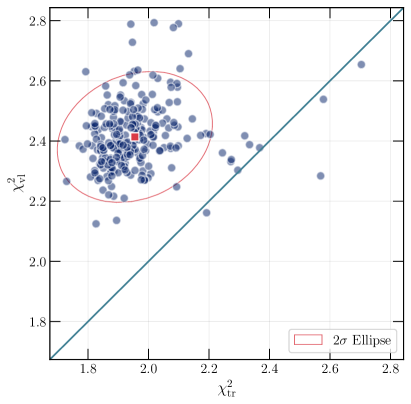
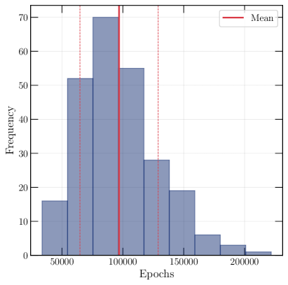
Figure 4.1: Left: distribution of the training $(\chi^{2}_{\rm tr})$ and validation $(\chi^{2}_{\rm vl})$ values for the fit error function $E_{\rm exp}^{(k)}$ over the $N_{\rm rep}=200$ replicas entering the NNSF$\nu$ data-driven parametrisation. We consider only the contribution from the experimental data in this comparison. The red square indicates the mean value over the replicas, while the red ellipse represents the $2\sigma$-contour. Right: the corresponding distribution of training lengths. The solid red line indicates the mean value while the dashed red lines indicate the $1\sigma$ standard deviation.

Fit performance.

Fig. 4.1 displays the distribution of the experimental training and validation error functions, $E^{(k)}_{\rm tr}$ and $E^{(k)}_{\rm val}$, evaluated over the $N_{\rm rep}=200$ Monte Carlo replicas used in the fit. The red square indicates the mean value over the replicas, while the red ellipse represents the $2\sigma$-contour. Since the validation datasets are not used for the optimisation, in general one expects the values of $E^{(k)}_{\rm val}$ to be somewhat higher than those of $E^{(k)}_{\rm tr}$, and indeed $\left\langle E_{\rm tr}\right\rangle\sim 2.0$ while $\left\langle E_{\rm val}\right\rangle\sim 2.4$. The replicas are clustered around the mean value and only a few outliers are present. Specifically, around 18 replicas fall outside the $2\sigma$-ellipse, to be compared with the 10 that would be expected to lie outside the 95% CL interval of a purely Gaussian distribution. As explained in Sect. 3.4, the post-fit procedure removes outlier replicas exhibiting $E_{\rm tr}^{(k)}$ or $E_{\rm val}^{(k)}$ values 4$\sigma$ away from the corresponding mean value.

The right panel of Fig. 4.1 shows the distribution of training lengths, defined as the number of epochs at which the optimal stopping conditions are reached, over the $N_{\rm rep}=200$ replicas. None of the replicas reach the maximum number of iterations (see Table 3.2), demonstrating that in all cases convergence is reached in a way that satisfies the cross-validation stopping criterion. Furthermore, the distribution is approximately Gaussian, with a mean of $N_{\rm ep}\sim 10^{5}$ epochs, and does not present any significant long tails. These two considerations point to a stable training which is evenly distributed among the replica distribution.

Fig. 4.2 displays the posterior probability distributions associated to the preprocessing exponents $\alpha_{i},\bar{\alpha}_{i}$ as defined in Eq. (3.2) for each of the fitted neutrino and antineutrino structure functions. Recall that these exponents are part of the fitted parameters and their values are restricted to the interval $\alpha_{i}\in\left[0,2\right]$. As in Fig. 4.1, the distribution is sampled from the $N_{\rm rep}=200$ replicas entering NNSF$\nu$. For each structure function, the distributions for the small-$x$ neutrino and antineutrino exponents, $\alpha_{i}$ and $\bar{\alpha}_{i}$ respectively, turn out to be similar, indicating that the small-$x$ behaviour of NNSF$\nu$ depends only mildly on the neutrino flavour. The fact that despite $\alpha_{i}$ and $\bar{\alpha}_{i}$ being fitted separately, the same distributions are obtained, is another indication of the fit stability, given that QCD predicts that asymmetries between neutrino and antineutrino structure functions are washed out in the small-$x$ region. The three structure functions also prefer similar small-$x$ preprocessing exponents, with median values of $\alpha_{1}\sim 1.25$, $\alpha_{2}\sim 1.1$, and $\alpha_{3}\sim 1.05$ for $F_{2}$, $xF_{3}$, and $F_{L}$ respectively, and in agreement within uncertainties. The distributions of $\alpha_{i},\bar{\alpha}_{i}$ are non Gaussian and exhibit a skewed tail towards smaller values of the exponents.

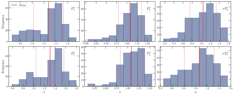
Figure 4.2: Posterior probability distributions for the preprocessing exponents $\alpha_{i},\bar{\alpha}_{i}$ as defined in Eq. (3.2) for each of the fitted neutrino and antineutrino structure functions. As in Fig. 4.1, the distribution is sampled from the $N_{\rm rep}=200$ replicas entering NNSF$\nu$. The vertical solid (dashed) lines indicate the mean values ($1\sigma$ ranges).

4.2 Comparison with data and previous calculations

Here we compare the NNSF$\nu$ results with other calculations of neutrino structure functions, in particular with BGR18 and Bodek-Yang, as well as with the YADISM predictions based on nNNPDF3.0 which enter the fit as the QCD boundary condition. We then show the agreement between NNSF$\nu$ and representative datasets used in the fit. Subsequently, we study the NNSF$\nu$ uncertainties and their dependence with respect to variations in the $x$, $Q^{2}$ and $A$ inputs of the parametrisation.

Comparison with Bodek-Yang and BGR18.

First, we compare the NNSF$\nu$ predictions with those from the Bodek-Yang and BGR18 calculations described in Sect. 2.2. In both cases, we access their predictions by means of their implementation in the GENIE event generator. For BGR18, we consider the variant based on NLO coefficient functions and NNPDF3.1 NLO as input PDF. We also display the YADISM predictions based on nNNPDF3.0 which enter the fit as the QCD boundary condition in Region II. The corresponding comparisons at the inclusive neutrino cross-section level will be presented in Sect. 5. We consider predictions for an isoscalar free-nucleon target, and also in Sect. 5 we will compare results for other nuclear targets for inclusive cross-sections.

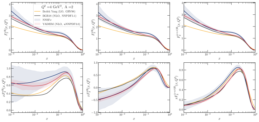
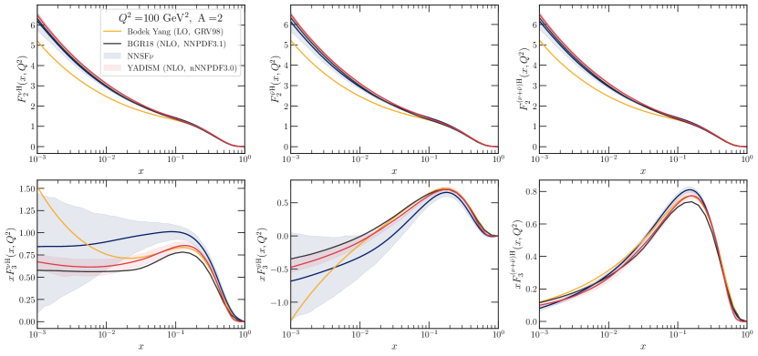
Figure 4.3: The NNSF$\nu$ predictions, together with the corresponding 68% CL uncertainties, as function of $x$ at $Q^{2}=4\leavevmode\nobreak\ \rm{GeV^{2}}$ (Region I, top panels) and $Q^{2}=100^{2}\leavevmode\nobreak\ \rm{GeV^{2}}$ (Region II, bottom panels). We display the $F_{2}$ and $xF_{3}$ structure functions for neutrinos, antineutrinos, and their sum on an isoscalar free-nucleon target (²H). The NNSF$\nu$ results are compared with the central values of the Bodek-Yang and BGR18 calculations, as well as with the YADISM calculation based on nNNPDF3.0 (with the red band indicating the PDF uncertainties).

Figs. 4.3 and 4.4 display the NNSF$\nu$ predictions as function of $x$ for $Q^{2}=4\leavevmode\nobreak\ \rm{GeV^{2}}$ (Region I) and $Q^{2}=100\leavevmode\nobreak\ \rm{GeV^{2}}$ (Region II) and then as a function of $Q$ for $x=0.0126$ and $x=0.25$, respectively. We display the $F_{2}$ and $xF_{3}$ structure functions for neutrinos, antineutrinos, and for their sum for an isoscalar free-nucleon target (²H). The error band on the NNSF$\nu$ predictions indicates the 68% confidence level intervals evaluated over the $N_{\rm rep}=200$ Monte Carlo replicas. We also consider the central values of the Bodek-Yang and BGR18 calculations, as well as the YADISM prediction including PDF uncertainties. For the BGR18 and YADISM calculations we only display results corresponding to the perturbative region with $Q^{2}>3.5\leavevmode\nobreak\ \rm{GeV^{2}}$. In Fig. 4.4, the area covered in light gray indicates the $Q^{2}$ coverage of Region II, where the NNSF$\nu$ parametrisation is constrained to reproduce the YADISM QCD boundary condition.

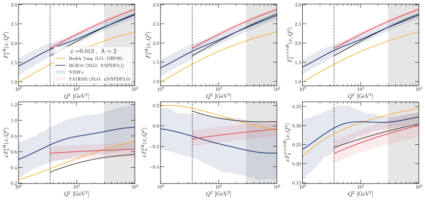
Figure 4.4: Same as Fig. 4.3 now as a function of $Q^{2}$ for $x=0.0125$ (upper) and $x=0.25$ (lower panels). The BGR18 and YADISM calculations are restricted to the region $Q^{2}\geq 3.5\leavevmode\nobreak\ \rm{GeV^{2}}$ (indicated by a dashed grey vertical line) to ensure the validity of perturbative QCD. The area covered in light gray indicates Region II, where the NNSF$\nu$ parametrisation is constrained by the YADISM boundary condition rather than by the experimental data.

From the comparisons in Figs. 4.3 and 4.4 one can observe how the NNSF$\nu$ predictions reproduce the YADISM boundary conditions at $Q^{2}=100\leavevmode\nobreak\ \rm{GeV^{2}}$ in the relevant region of $x$. We verify that within the whole Region II there is agreement within uncertainties between NNSF$\nu$ and YADISM, demonstrating that as required the QCD boundary condition is being reproduced by the structure function parametrisation. At medium and small-$x$, there is a good agreement between the BGR18 calculation and the NNSF$\nu$ predictions in the region of validity of the former (for $Q^{2}\geq 4\leavevmode\nobreak\ \rm{GeV^{2}}$), with some differences in the large-$x$ region. It is interesting to note that the agreement found between NNSF$\nu$ and YADISM in Region II is not automatic: for instance at $Q=2$ GeV (Region I), we find that for $x\in\left[0.05,0.3\right]$ the two results disagree within uncertainties, showing that the experimental neutrino data (rather than the QCD boundary condition) is driving the fit results there.

Furthermore, one observes from these comparisons how the Bodek-Yang calculation falls outside the $1\sigma$ error band of the NNSF$\nu$ prediction for a significant region of the relevant $x$ and $Q^{2}$ values, in particular for $F_{2}$ at small- and large-$x$. For instance, for $x\simeq 0.25$ in the low-$Q$ region, the Bodek-Yang prediction is around 25% smaller than the NNSF$\nu$ one. The agreement between the NNSF$\nu$ and Bodek-Yang structure functions improves for heavier nuclei, as we will demonstrate in Sect. 5 when evaluating the inclusive neutrino cross-sections on iron, tungsten, and lead targets.

Another interesting feature of Figs. 4.3 and 4.4 is the behaviour of NNSF$\nu$ in the extrapolation regions. Concerning the $x$ dependence, the NNSF$\nu$ uncertainties increase at small-$x$ specially at low-$Q$ due to the lack of direct experimental data, while in the same $x$ region at higher values of $Q$ these uncertainties are reduced due to the information provided by the QCD boundary condition. Note that in the case of the $xF_{3}$ structure function, the small-$x$ behaviour is fixed in the case of the $\nu+\bar{\nu}$ combination, rather than for the individual $\nu$ and $\bar{\nu}$ structure functions. Concerning the extrapolation in $Q^{2}$, the NNSF$\nu$ uncertainties increase as $Q^{2}$ decreases due to the lack of data, and decrease as $Q^{2}$ increases as a consequence of the constraints from the QCD boundary condition.

Comparisons with experimental data.

The values of the $\chi^{2}_{\rm exp}$ reported in Table 4.1 indicate good agreement between the experimental data and the NNSF$\nu$ parametrisation. This agreement can be further illustrated by comparing the NNSF$\nu$ predictions with representative datasets entering the fit in Region I in selected kinematic regions as a function of $Q^{2}$, as done in Fig. 4.5. For each dataset we also indicate the values of $x$ and $A$ for the bin shown. For the experimental data points, the error band corresponds to the diagonal entry of the associated covariance matrix. Specifically, we show the $F_{2}$ and $xF_{3}$ structure functions (averaged over $\nu$ and $\bar{\nu}$) for the BEBCWA59, CHARM, and CCFR experiments. A similar level of agreement is obtained for the various regions of $x$, $Q^{2}$, or $A$ considered in this analysis, again indicating a well-balanced fit where the different kinematic regions are satisfactorily described.

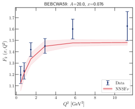
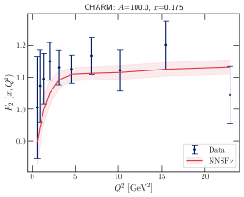
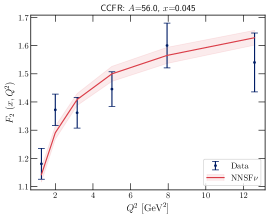
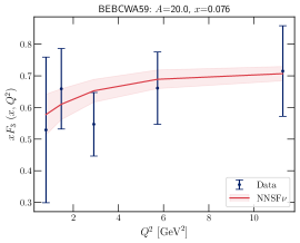
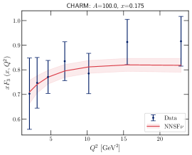
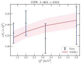
Figure 4.5: Comparison between a representative subset of the experimental data entering the fit in Region I and the corresponding NNSF$\nu$ predictions as a function of $Q^{2}$. For each dataset we also indicate the values of $x$ and $A$ corresponding to the bin shown. The uncertainty band in NNSF$\nu$ is the standard deviation over the $N_{\rm rep}=200$ Monte Carlo replicas. For the experimental data, the error band corresponds to the diagonal entry of the covariance matrix. From top to bottom we show the $F_{2}$ and $xF_{3}$ structure functions (averaged over $\nu$ and $\bar{\nu}$) for the BEBCWA59, CHARM, and CCFR experiments.

Uncertainty estimate and kinematic dependence.

Concerning the uncertainty estimate of the NNSF$\nu$ determination, in general its $1\sigma$ errors are found to be rather smaller as compared those of the corresponding experimental measurements, see also Fig. 4.5. This behaviour is expected, since effectively the neural network parametrisation is averaging over the input data [63] which displays partly overlapping kinematic coverage. In addition, one has to account for the effects of the QCD boundary conditions, and indeed one can verify that as the lower boundary of Region II ($Q_{\rm dat}$) is approached, the NNSF$\nu$ uncertainties decrease as a consequence of these constraints. These effect are illustrated in Figs. 4.6 and 4.7, which display the absolute 68% CL relative uncertainties in the NNSF$\nu$ structure functions as $Q^{2}$ is varied for $x=0.25$ and as $x$ is varied for $Q^{2}=2$ GeV², respectively. We compare the uncertainties for the isoscalar free nucleon ²H target with those for Ne, Fe, and Pb targets, for the three structure functions and different initial states.

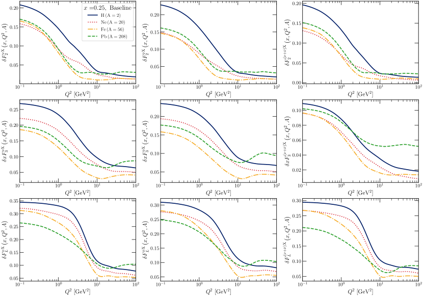
Figure 4.6: The 68% CL (absolute) uncertainties in the NNSF$\nu$ baseline fit as a function of $Q^{2}$ in the region between 1 GeV² and 100 GeV² for $x=0.25$. We compare the results of an isoscalar nucleus ${}^{2}\mathrm{H}$ with those corresponding to various nuclear targets entering the fit, namely ${}^{20}\mathrm{Ne}$, ${}^{56}\mathrm{Fe}$, and ${}^{208}\mathrm{Pb}$. We display results for the three structure functions $F_{2},xF_{3},$ and $F_{L}$, separately for the $\nu$, $\bar{\nu}$ and $\nu+\bar{\nu}$ initial states.

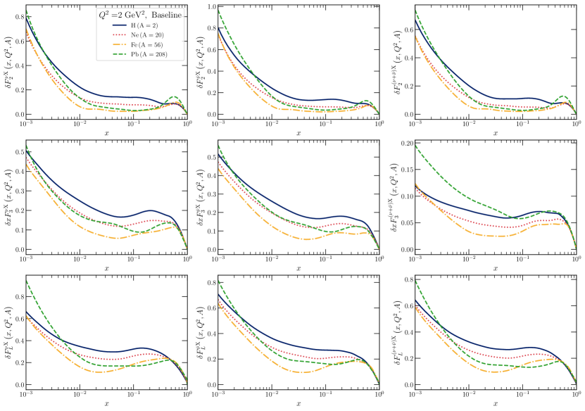
Figure 4.7: Same as Fig. 4.6 now as a function $x$ for $Q^{2}=2\leavevmode\nobreak\ \rm{GeV^{2}}$

The uncertainties of the NNSF$\nu$ determination stabilize in Region II, where they approach those of the QCD boundary condition based on YADISM and nNNPDF3.0. In Region II, the $Q^{2}$ dependence of the absolute uncertainties is moderate and arising from scaling violations. In the low-$Q^{2}$ extrapolation region, the NNSF$\nu$ uncertainties increase as a consequence of the limited experimental constraints, as also mentioned above. Uncertainties also increase as $x$ decreases, both for $F_{2}$ (which rises at small-$x$) as for $xF_{3}$ (which being a non-singlet does not). Lastly, the NNSF$\nu$ uncertainties become small in the large-$x$ region where structure functions vanish due to the elastic limit.

Another noticeable feature from Figs. 4.6 and 4.7 is the dependence of the NNSF$\nu$ uncertainties with respect to the atomic mass number $A$. At low $Q$ values (Region I), uncertainties are the largest for ²H, consistent with the fact that there is no experimental information in this region. As $Q$ is increased, the NNSF$\nu$ uncertainties for all nuclei become similar, specially for the $F_{2}$ and $F_{L}$ structure functions. In general, the most precise NNSF$\nu$ prediction is obtained for an iron target, at least in the region of $x$ and $Q^{2}$ being shown, which is consistent with the fact that Fe is the most abundant target in the input dataset. However, we point out that this is not the case in the small-$x$ region with $x\mathrel{\hbox to0.0pt{\lower 4.0pt\hbox{\hskip 1.0pt$\sim$}\hss}\raise 1.0pt\hbox{$<$}}10^{-5}$, since there are no constraints from $D$-meson production on an Fe target, and hence for the UHE neutrino cross-sections the uncertainties on a Fe target are higher than those of either a ²H or a Pb target as shown in Sect. 5.2.

4.3 Stability and validation

We now study the stability of the NNSF$\nu$ determination by comparing the baseline fit with variants where either the input dataset or some aspect of the fitting methodology are modified. In particular, we assess the dependence of the fit on the value of the threshold scale $Q^{2}_{\rm dat}$ separating Regions I and II; quantify its stability when double-differential cross-section data is replaced with their structure functions $(F_{2},xF_{3})$ counterparts; and assess the quality of the NNSF$\nu$ interpolation to values of the atomic mass number $A$ not considered in the fit.

Dependence on the matching scale.

Fig. 4.8 compares the NNSF$\nu$ baseline results with a fit variant in which the matching scale between Regions I and II has been increased from $Q^{2}_{\rm dat}=30\leavevmode\nobreak\ \rm{GeV^{2}}$ (just above the bottom mass) to $Q^{2}_{\rm dat}=50\leavevmode\nobreak\ \rm{GeV^{2}}$ . Results are shown at $Q^{2}=40$ GeV² as a function of $x$ for both Fe and Pb targets, and are normalised to the central NNSF$\nu$ baseline. We display results for the three structure functions separately for neutrinos, antineutrinos, and for their sum. One finds that, in all cases considered, this NNSF$\nu$ variant is in agreement with the baseline fit within uncertainties, demonstrating the fit stability with respect to variations of the $Q^{2}_{\rm dat}$ threshold value.

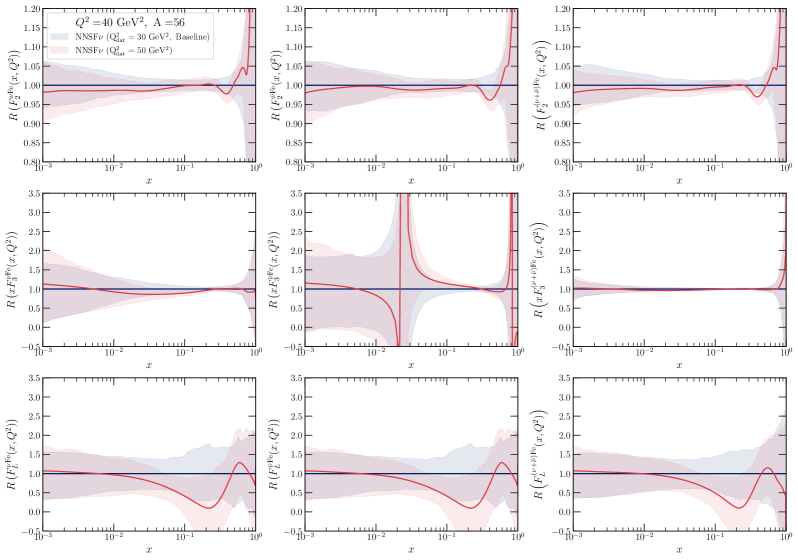
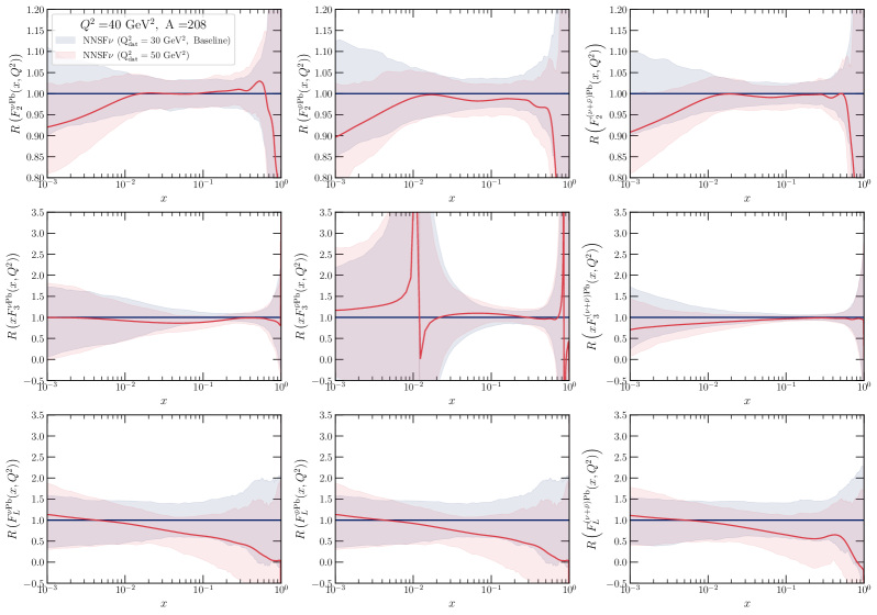
Figure 4.8: Comparison of the neutrino structure functions at $Q^{2}=40$ GeV² as a function of $x$ in the NNSF$\nu$ baseline fit, where $Q^{2}_{\rm dat}=30\leavevmode\nobreak\ \rm{GeV^{2}}$, with a variant in which Region I is extended up to $Q^{2}_{\rm dat}=50\leavevmode\nobreak\ \rm{GeV^{2}}$, normalised to the central value of the baseline. We show results for Fe (top) and Pb (bottom panels) targets for the three structure functions $F_{2},xF_{3},$ and $F_{L}$ separately for the $\nu$, $\bar{\nu}$ and $\nu+\bar{\nu}$ initial states.

This stability is particularly visible for $F_{2}$ and $xF_{3}$, while somewhat larger effects are observed for $F_{L}$ in the large-$x$ region. The likely explanation of this effect is that experimental constraints on $F_{L}$ are limited and hence this structure function is more sensitive to the settings of the matching to the QCD predictions. Some differences are also observed for the lead structure function $F_{2}$ for $x\mathrel{\hbox to0.0pt{\lower 4.0pt\hbox{\hskip 1.0pt$\sim$}\hss}\raise 1.0pt\hbox{$<$}}0.01$. In the case of this target the direct experimental constraints end at $x\approx 0.025$, so again the matching scale has some influence on the results. Nevertheless, agreement within uncertainties is preserved in all cases, demonstrating that the NNSF$\nu$ analysis is robust with respect to moderate variations of the hyperparameter $Q^{2}_{\rm dat}$. This said, as discussed in Sect. 3.1, $Q^{2}_{\rm dat}$ can neither be arbitrarily reduced, which would cut away most of the neutrino data, nor increased, since a gap would arise between the data region and the region where QCD boundary conditions are imposed.

Reduced cross-sections vs structure functions.

Fig. 4.9 presents the same comparison as that in Fig. 4.8 now for a NNSF$\nu$ fit variant in which the data on the double-differential cross-sections for the CDHSW, CHORUS, and NuTeV experiments has been replaced by the corresponding measurements at the level of the individual structure function $F_{2}$ and $xF_{3}$, see also the discussion in Sect. 3.2. We note that since in these experiments the separate structure functions are extracted from the differential cross-sections by means of a theory-assisted averaging procedure, this replacement entails removing 3805 cross-section data points and replace them by a much smaller number, 490, of structure functions data points.

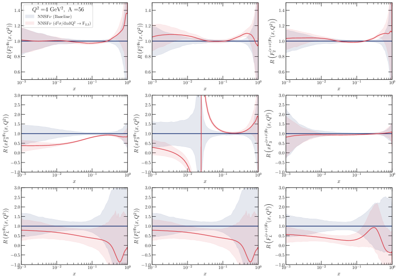
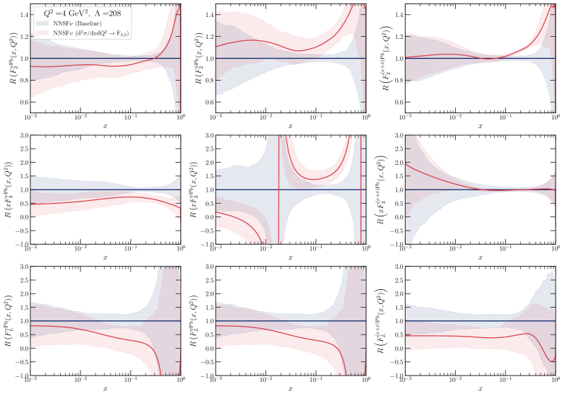
Figure 4.9: Same as Fig. 4.8 for the NNSF$\nu$ fit variant in which the data on double-differential cross-sections for the CDHSW, CHORUS, and NuTeV experiments has been replaced by the corresponding measurements at the $\left(F_{2},xF_{3}\right)$ structure function level.

In terms of the fit quality, from the outcome of this fit variant we find a marked deterioration of the $\chi^{2}_{\rm exp}$, which increases to $1.450$ as compared to the value of 1.287 for the baseline (see Table 4.1). This fit quality worsening can be traced back to the effect of the CHORUS and NuTeV experiments in particular, where for instance the $F_{2}$ structure function data has $\chi^{2}_{\rm exp}=2.073$ and 2.445 per data point respectively. We note that the poor fit quality to the NuTeV $F_{2}$ and $xF_{3}$ structure function data has already been reported and studied in the literature (see [95, 96, 97] and references therein), and concerns about the internal consistency of this dataset have been raised. While our choice of reduced cross-sections $d^{2}\sigma/dxdQ^{2}$ for the baseline dataset is motivated by a priori considerations based on it being a more robust, less theory-dependent observable, the poor description of the $F_{2}$ data from CHORUS and NuTeV provides a further argument in favour of the choice adopted here.

Concerning the impact that this dataset variation has at the level of the NNSF$\nu$ output, from Fig. 4.9 we find that in general results are compatible at the one-sigma level, specially when considering structure functions averaged over neutrinos and antineutrinos. Nevertheless, non-negligible differences, not covered by the respective uncertainties, are observed for instance for $F_{2}^{\bar{\nu}}$ at large-$x$ both for Fe and Pb, for $xF_{3}$ for $A=56$ (the NuTeV target) when separated into neutrino and antineutrino predictions, and for $F_{L}$ for intermediate $x$ and also for $A=56$. We note that in the latter case, this fit variant does not include direct experimental constraints on $F_{L}$ and hence the only information provided by the fit comes from the QCD boundary conditions in Region II.

Taking into account both the deterioration at the fitted $\chi^{2}_{\rm exp}$ level, the lack of agreement in the fitted structure functions for specific regions of $(x,Q^{2},A)$, and their poor description when the baseline NNSF$\nu$ predictions are used, one concludes the separate $F_{2}$ and $xF_{3}$ structure functions are not equivalent, and may be inconsistent, as compared with their differential cross-sections counterparts which is our default choice. Even so, we note that at the level of $F_{2}$ and $xF_{3}$ averaged over neutrinos and antineutrinos, except for $F_{2}$ at $x\mathrel{\hbox to0.0pt{\lower 4.0pt\hbox{\hskip 1.0pt$\sim$}\hss}\raise 1.0pt\hbox{$>$}}0.2$, the baseline and the variant fits are in agreement at the 68% CL and hence predictions obtained from them, for instance for inclusive cross-sections, are also likely to be in agreement, the only possible exception being low $E_{\nu}$ values where the large-$x$ region dominates.

Interpolation in atomic number $A$.

One of the key advantages of the NNSF$\nu$ strategy is the ability to interpolate the predictions for neutrino structure functions to other targets, with different atomic mass numbers, beyond those directly considered in the fit and that may be relevant for neutrino phenomenology, such as oxygen ($A=16$), argon ($A=39$), calcium ($A=40$), and tungsten ($A=184$) among others.

Here we validate the NNSF$\nu$ interpolation in $A$ by comparing the baseline fit with two variants. First, we compare the baseline fit results with those of a variant in which the datasets with atomic mass number $A\simeq 20$, namely BEBCWA59 (Ne) and CHARM (CaCO₃), are excluded. In such case, the predictions for $A=20$ of the fit variant in Region I will be obtained from a extrapolation of the constraints provided by the fitted data with $A\geq 56$ for iron and lead targets. Second, we compare the NNSF$\nu$ predictions from the baseline fit in Region II with the YADISM+nNNPDF3.0 calculations for calcium $(A=40)$, a nuclear species which is not contained in the baseline analysis. These two tests make possible validating the interpolation (and extrapolation) of the NNSF$\nu$ predictions to new values of $A$ not used in the fit neither in Region I nor in Region II.

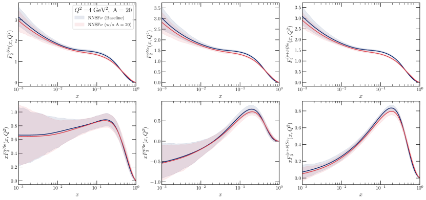
Figure 4.10: Comparison between the results of the NNSF$\nu$ baseline fit and those of a fit variant in which the data from the $A\simeq 20$ datasets, BEBCWA59 (Ne) and CHARM (CaCO₃), are excluded. We display the $F_{2}$ and $xF_{3}$ structure functions for $A=20$ for $Q^{2}=4$ GeV² as a function of $x$, separately for the neutrino, antineutrino, and their sum initial states. In this kinematic region, the predictions for $A=20$ of the fit variant are obtained from extrapolating the constraints provided by the fitted data with $A\geq 56$ (for iron and lead targets).

First, Fig. 4.10 displays the results comparing the baseline fit with the variant in which the $A\simeq 20$ datasets, namely BEBCWA59 (Ne) and CHARM (CaCO₃), are excluded. We display the $F_{2}$ and $xF_{3}$ structure functions for $A=20$ for $Q^{2}=4$ GeV² as a function of $x$, separately for the neutrino, antineutrino, and their sum initial states. In this kinematic region, the predictions for $A=20$ of the NNSF$\nu$ variant arise entirely from extrapolating the constraints provided by the fitted data with $A\geq 56$ for iron and lead targets. As one can observe from the comparison, the two fits are compatible within the respective uncertainties, with the possible exception of $F_{2}^{\nu A}$ for $x\simeq 0.2$ where the baseline and its variant overlap at the $2\sigma$ level. The good agreement between the baseline fit and its variant, specially for $F_{2}$ for $x\mathrel{\hbox to0.0pt{\lower 4.0pt\hbox{\hskip 1.0pt$\sim$}\hss}\raise 1.0pt\hbox{$<$}}0.1$ and for $xF_{3}$, confirms that the methodology extrapolates in the atomic mass number $A$ in a way that is consistent with the available experimental constraints in Region I, and that the predicted structure functions are stable upon removal of a subset of the fitted datasets.

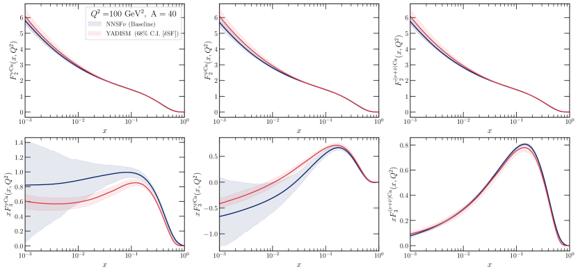
Figure 4.11: Same as Fig. 4.10, now for the structure functions of an $A=40$ target comparing the outcome of NNSF$\nu$ with that of YADISM (with nNNPDF3.0 as input). We display results at $Q^{2}=100\leavevmode\nobreak\ \rm{GeV^{2}}$ as a function of $x$. Since neither the fitted data (in Region I) nor the QCD boundary conditions (in Region II) include information on $A=40$, this comparison tests the interpolation of NNSF$\nu$ to $A$ values not considered in the fit. The error band in the YADISM predictions contains the PDF uncertainties, but not the MHOU ones.

Fig. 4.11 then compares the NNSF$\nu$ predictions for $A=40$ with the corresponding YADISM calculations, with nNNPDF3.0 as input, for a calcium $\left({}^{40}\mathrm{Ca}\right)$ target. As in Fig. 4.10, we compare the $F_{2}$ and $xF_{3}$ neutrino structure functions but this time at $Q^{2}=100\leavevmode\nobreak\ \rm{GeV^{2}}$, which corresponds to Region II. Since neither the fitted data (in Region I) nor the QCD boundary conditions (in Region II) include information on $A=40$, this comparison assesses the interpolation capabilities of NNSF$\nu$ to atomic mass numbers not considered in the fit. The error band in the YADISM predictions of Fig. 4.11 contains the PDF uncertainties but not the MHOU ones.

One finds that the interpolated predictions of NNSF$\nu$ for $A=40$ are in very good agreement with the YADISM calculation, which do not enter the fit. While excellent agreement can be seen at the averaged level, some differences are noticed when looking at large-$x$ of the separate $\nu$- and $\bar{\nu}$-results for $xF_{3}$. These discrepancies could however be attributed to the small constraints on the sea-quark distributions that cancel out when taking the average. This result implies that the NNSF$\nu$ parametrisation interpolates in $A$ in a manner consistent with the underlying behaviour of the QCD prediction in Region II, and furthermore that the fit results would not be affected in the case that QCD data with $A=40$ is added to the NNSF$\nu$ fit. These results demonstrate that NNSF$\nu$ is able to reliably interpolate between nuclear targets and therefore capable of providing predictions for $A$ values for which no direct experimental measurements are available. We use this feature to provide LHAPDF sets for all values of $A$ relevant for neutrino phenomenology as listed in App. A.

4.4 The Gross-Llewellyn Smith sum rule

Finally, we use the NNSF$\nu$ determination to evaluate the Gross-Llewellyn-Smith sum rule of neutrino structure functions, Eq. (2.16), and assess its agreement with respect to the perturbative QCD calculation. The latter prediction indicates that for an isoscalar target $A$ one expects to find

$$\int_{0}^{1}{{dx}\over{x}}xF_{3}^{\nu A}(x,Q^{2})=3\left(1+\sum_{k=1}^{3}\left({{\alpha_{s}(Q^{2})}\over{\pi}}\right)^{k}c_{k}(n_{f})\right)\,,$$ (4.1)

with $n_{f}$ being the number of active flavours at the scale $Q^{2}$ and the coefficients $c_{k}$ known up to third order in perturbation theory. Evaluating Eq. (4.1) requires extrapolating down to the $x\to 0$ region which is not accessible experimentally, and hence instead we compute a truncated variant of the GLS sum rule,

$${\rm GLS}\left(Q^{2},A,x_{\rm min}\right)\equiv\int_{x_{\rm min}}^{1}{{dx}\over{x}}xF_{3}^{\nu A}(x,Q^{2})\,,$$ (4.2)

for different values of the lower integration limit $x_{\rm min}$ and the atomic mass number $A$. The truncated sum rule Eq. (4.2) should converge to the QCD prediction in Eq. (4.1) in the $x_{\rm min}\to 0$ limit. Furthermore, the GLS sum rule should hold true irrespective of the value of the mass number $A$ entering the calculation.

Fig. 4.12 displays the outcome of the calculation of the (truncated) Gross-Llewellyn-Smith sum rule, Eq. (4.2), evaluated with the NNSF$\nu$ baseline fit as a function of $Q^{2}$. We display results corresponding to lower integration limits of $x_{\rm min}=10^{-3}$ and of $10^{-4}$ for $A=1$, $A=40$, and $A=56$ nuclei. We compare the NNSF$\nu$ baseline truncated results with the corresponding QCD predictions for the exact GLS sum rule. Note that the latter is the same in all panels, since it is independent of both $x_{\rm min}$ and $A$, and that its $Q^{2}$ dependence is entirely dictated by that of the running of the strong coupling $\alpha_{s}(Q^{2})$. As in the rest of this section, the uncertainty in the NNSF$\nu$ results is computed as the 68% CL intervals from the $N_{\rm rep}=200$ replicas that constitute the representation of its probability density.

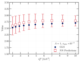
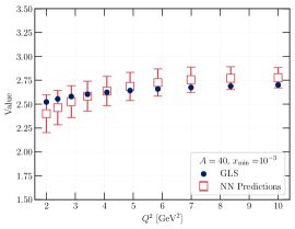
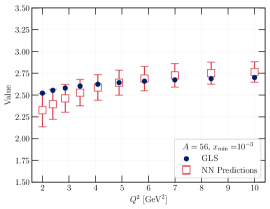
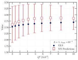
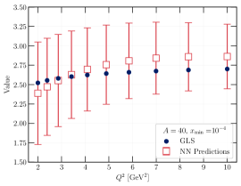
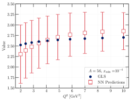
Figure 4.12: The Gross-Llewellyn-Smith sum rule evaluated as a function of $Q^{2}$. The predictions of NNSF$\nu$ are compared with the perturbative QCD calculation evaluated at N³LO. We display results corresponding to a lower integration limit of $x_{\rm min}=10^{-3}$ (top) and of $x_{\rm min}=10^{-4}$ (bottom panels) for $A=1$ (left), $A=40$ (middle), and for $A=56$ (right panel). Note that the QCD prediction for the GLS sum rule is the same in all panels, since it is independent of both $x_{\rm min}$ and $A$.

From this comparison, one can conclude that there is agreement within uncertainties between the (truncated) calculation of the GLS sum rule from the phenomenological NNSF$\nu$ determination of the $xF_{3}$ neutrino structure function and the corresponding perturbative QCD prediction. The agreement in central values, especially in the large-$Q^{2}$ region, slightly deteriorates once $x_{\rm min}$ is reduced from $10^{-3}$ to $10^{-4}$. But at the same time, the uncertainties in the truncated sum rule calculation increase as $x_{\rm min}$ decreases, as expected since NNSF$\nu$ does not have direct experimental constraints below $x\simeq 0.01$, see also Table 3.1. Even more remarkably, not only the value but also the slope with $Q^{2}$, which in the QCD calculation is dictated by the $\alpha_{s}(Q)$ running, is correctly reproduced by the data-driven NNSF$\nu$ analysis. The analysis of Fig. 4.12 hence indicates that the NNSF$\nu$ data-driven determination of $xF_{3}$ is consistent with the QCD expectations, and in particular that extrapolates to the small-$x$, low-$Q^{2}$ region in a manner which improves the agreement with the N³LO result given by Eq. (4.1).

The agreement between the truncated GLS sum rule computed with NNSF$\nu$ and the QCD calculation holds true for the three values of $A$ considered, namely $A=1,40$, and $56$. The main effect of the $A$ dependence appears to be the increase in the uncertainties in the $A=1$ case as compared to the heavier nuclei, due to the lack of direct experimental constraints on light nuclear targets. This insensitivity of the results of the truncated GLS sum rule with respect to the value of $A$ is consistent with the expectation that this sum rule is related to the nucleon valence sum rules, which are satisfied and take the same values irrespective of the value of $A$ entering the calculation of the neutrino structure functions.

5 Inclusive neutrino cross sections

Here we deploy the NNSF$\nu$ determination of neutrino structure functions to evaluate inclusive neutrino scattering cross sections as a function of $E_{\nu}$ for different projectiles and targets. Specifically, we provide predictions for the complete range of energies relevant for neutrino phenomenology, from the GeV region entering accelerator experiments up to the multi-EeV energies of cosmic neutrinos. Our predictions come accompanied with an estimate of the dominant uncertainties relevant in each energy region.

First, we compare the NNSF$\nu$ determination with previous results in the literature, in particular with the Bodek-Yang, BGR18, and CSMS11 calculations. We evaluate the mean inelasticity $\left\langle y\right\rangle$ for different neutrino energies, compare with experimental measurements of the inclusive cross-section from NuTeV, assess the sensitivity of our calculation to the low-$Q$ region, and quantify the impact of nuclear corrections for the most relevant target materials. Furthermore, we provide dedicated predictions for the energy range and target materials required for the interpretation of far-forward neutrino scattering experiments at the LHC.

5.1 The NNSF$\nu$ cross sections

Starting from the double-differential neutrino-nucleus scattering cross sections of Eqns. (2.5) and (2.6), the inclusive cross section is obtained [41] by integrating over the kinematically allowed range in $x$ and $Q^{2}$,

$$\sigma^{\nu N}(E_{\nu})=\int_{Q^{2}_{\rm min}}^{Q^{2}_{\rm max}}{\rm d}Q^{2}\left[\int_{x_{0}(Q^{2})}^{1}{\rm d}x{{{\rm d}^{2}\sigma^{\nu N}}\over{{\rm d}x{\rm d}Q^{2}}}(x,Q^{2},y)\right]\,,$$ (5.1)

where the integration limits are given by

$$Q^{2}_{\rm max}=2m_{N}E_{\nu}\,,\qquad x_{0}(Q^{2})={{Q^{2}}\over{2m_{N}E_{\nu}}}\,,$$ (5.2)

and with the inelasticity related to the neutrino energy by $y=Q^{2}/(2m_{N}xE_{\nu})$. In an inclusive calculation, the lower integration limit $Q^{2}_{\rm min}$ should go all the way down to $Q^{2}_{\rm min}=0$. While most previous studies impose a cut in $Q^{2}_{\rm min}$ to restrict the integration in Eq. (5.1) to the perturbative region, this is not required within the NNSF$\nu$ approach since our structure function predictions are valid for all $Q^{2}$ values.

For the calculations presented in this section we take $Q_{\rm min}=0.03$ GeV and study the dependence of the predictions with respect to variations of this choice. A kinematic cut in the final-state invariant mass of $W\geq 2$ GeV is applied to restrict the calculation to the inelastic scattering region. See App. A for technical details about the implementation of Eq. (5.1) and the estimate of the associated uncertainties.

Comparison with Bodek-Yang, BGR18, and CSMS11.

Fig. 5.1 displays the ratio of the inclusive neutrino-nucleus inelastic cross section, Eq. (5.1), over the neutrino energy $E_{\nu}$ as a function of the latter. The NNSF$\nu$ prediction for the ratio $\sigma^{\nu N}/E_{\nu}$, together with the associated 68% CL uncertainty band is compared with the central values of the Bodek-Yang, BGR18, and CSMS11 calculations. The top panels display the absolute predictions for neutrinos and antineutrinos scattering on deuterium (understood here as isoscalar ²H without nuclear effects), iron, and lead targets. The bottom panels show the corresponding ratios for neutrinos, antineutrinos, and their sum with respect to the central NNSF$\nu$ baseline. The ratio $\sigma^{\nu N}/E_{\nu}$ is provided in units of $10^{-38}$ cm²/GeV per nucleon, hence assuming the proton and neutron content of the average nucleon in the target nuclei. We display neutrino energies from $E_{\nu}\simeq 10$ GeV up to $E_{\nu}\simeq 10^{11}\leavevmode\nobreak\ {\rm GeV}=100\leavevmode\nobreak\ {\rm EeV}$.

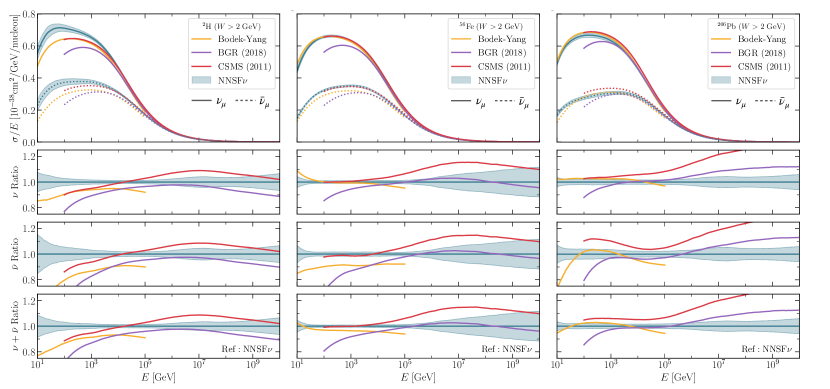
Figure 5.1: The inclusive neutrino-nucleus inelastic cross section, Eq. (5.1), divided by the neutrino energy $E_{\nu}$ as a function of the latter. The NNSF$\nu$ prediction, together with the associated 68% CL uncertainty band, is compared with the central values of the Bodek-Yang, BGR18, and CSMS11 calculations. The top panels displays the results for neutrinos and antineutrinos scattering on deuterium (left), iron (middle), and lead (right panel) targets. The bottom panels display the corresponding ratios for neutrino, antineutrino, and their sum with respect to the central value of the NNSF$\nu$ baseline calculation. We display the energy region covering from $E_{\nu}=10$ GeV up to $E_{\nu}=10^{11}\leavevmode\nobreak\ {\rm GeV}$.

The NNSF$\nu$ determination is the only available theory prediction applicable in the complete range of $E_{\nu}$ relevant for neutrino phenomenology. The region of formal applicability of the BY calculation is $E_{\nu}\leq 10^{5}$ GeV, while CMS11 and BGR18 are restricted to $E_{\nu}>100$ GeV. Furthermore, BGR18 was optimised to high-energy scattering and does not provide a good description of the energy region sensitive to low-$Q$ values. In the comparisons of Fig. 5.1, the CMS11 and BGR18 predictions are provided for a free isoscalar target and hence do not account for nuclear modification effects. The latter could be included by means of an external nuclear PDF analysis within a factorised approach, but only in the perturbative QCD region. Nuclear corrections are data-driven and model-independent in NNSF$\nu$, while they are model-dependent and neglect the constraints from proton-ion collisions at the LHC in the Bodek-Yang case. These nuclear effects are specially significant for heavy nuclei such as lead, as we discuss below.

The uncertainty band of the NNSF$\nu$ prediction varies from a few percent up to a maximum of 15%, depending on $E_{\nu}$ and the nuclear target. At low energies, it is the largest for ²H, given the lack of direct experimental constraints on low-$Q$ neutrino-hydrogen structure functions. At very high energies, it is the largest in iron since both for a free nucleon and for a lead target the nNNPDF3.0-based calculation accounts for the constraints on small-$x$ PDFs provided by charm production at LHCb. On the intermediate energy region with 100 GeV $\mathrel{\hbox to0.0pt{\lower 4.0pt\hbox{\hskip 1.0pt$\sim$}\hss}\raise 1.0pt\hbox{$<$}}E_{\nu}\mathrel{\hbox to0.0pt{\lower 4.0pt\hbox{\hskip 1.0pt$\sim$}\hss}\raise 1.0pt\hbox{$<$}}100$ TeV, uncertainties in the NNSF$\nu$ calculation of the inclusive cross-sections are at the few percent level at most.

Concerning the comparison between NNSF$\nu$ and the theory predictions from other groups, starting with the case of lead nuclei one observes agreement within uncertainties with the Bodek-Yang calculation for $E_{\nu}\mathrel{\hbox to0.0pt{\lower 4.0pt\hbox{\hskip 1.0pt$\sim$}\hss}\raise 1.0pt\hbox{$<$}}10$ TeV, except for antineutrinos with very low energies. For higher energies, NNSF$\nu$ agrees with BGR18 for energies above 1 TeV up to $10^{6}$ TeV, with the latter overshooting the former for $E_{\nu}\geq 10^{6}$ TeV due to the missing nuclear corrections related to the strong small-$x$ quark and gluon shadowing in lead nuclei found in nNNPDF3.0. The differences with CSMS11 at high energies are explained from the absence of nuclear effects, the choice of proton PDFs and the corresponding small-$x$ behaviour, and the treatment of top quark mass effects, see the discussion of [41, 22].

In the case of an iron target, there is also good agreement between NNSF$\nu$ and the Bodek-Yang predictions for neutrinos, while for antineutrinos the latter is suppressed by a factor around 10%. As demonstrated below in Fig. 5.2, the NNSF$\nu$ antineutrino predictions on Fe are preferred by the NuTev measurements of the inclusive cross-sections. In the case of the $\nu+\bar{\nu}$ sum, the differences between NNSF$\nu$ and BY are relatively moderate. The NNSF$\nu$ predictions are consistent with BGR18 for $E_{\nu}\mathrel{\hbox to0.0pt{\lower 4.0pt\hbox{\hskip 1.0pt$\sim$}\hss}\raise 1.0pt\hbox{$>$}}100$ TeV, as expected from the use of common settings for the QCD structure functions and the similarities in the input (n)PDFs, given that no strong nuclear small-$x$ shadowing effects have been identified in the case of lead. The CSMS11 calculation agrees with NNSF$\nu$ until around 10 TeV, and then overshoots it for the reasons discussed in the case of lead [41, 22].

Finally, concerning the isoscalar free-nucleon target ²H, NNSF$\nu$ predicts a larger cross-section as compared to Bodek-Yang by a factor between 10% and 20%, depending on the $E_{\nu}$ value. For this target, there exist no direct experimental constraints on neutrino-nucleon scattering, and hence in NNSF$\nu$ the $A=1$, low-$Q$ behaviour arises from the extrapolation from the data with $A\mathrel{\hbox to0.0pt{\lower 4.0pt\hbox{\hskip 1.0pt$\sim$}\hss}\raise 1.0pt\hbox{$>$}}20$ included in the fit and from the QCD constraints in Region II for $Q\geq Q_{\rm thr}$ with $A=1$. Despite the absence of direct constraints, thanks to the NNSF$\nu$ matching procedure for energies within $E_{\nu}\mathrel{\hbox to0.0pt{\lower 4.0pt\hbox{\hskip 1.0pt$\sim$}\hss}\raise 1.0pt\hbox{$>$}}1$ TeV a reliable prediction can be obtained by means of the perturbative QCD calculation using the reasonably accurate proton PDFs. In this high-energy region, the NNSF$\nu$ prediction is bracketed by the CSMS11 from above and BGR18 from below. The differences with BGR18 are explained by a combination of the input PDFs and the treatment of top quark mass effects [22], since NNSF$\nu$ uses FFNS5 and BGR18 is based on FONLL instead, see also Sect. 2.

Nevertheless, neutrino cross-sections on a free-nucleon target are of limited phenomenological interest due to the absence of data for this target material. This said, the large spread in the theory predictions for a free-nucleon target motivates future experimental analyses of neutrino scattering in the region $E_{\nu}\mathrel{\hbox to0.0pt{\lower 4.0pt\hbox{\hskip 1.0pt$\sim$}\hss}\raise 1.0pt\hbox{$<$}}1$ TeV with data taken on hydrogen, deuterium, or other light nuclei as targets.

Comparison with experimental data.

Several experiments have measured the inclusive neutrino-nucleus interaction cross section for different nuclear targets and energy ranges. To further validate the NNSF$\nu$ predictions on neutrino cross-section measurements, Fig. 5.2 compares NNSF$\nu$ with the NuTeV [83] experimental data on inclusive neutrino cross sections an iron target, separately for neutrinos and antineutrinos. We focus on the energy region (between 20 GeV and 380 GeV) relevant for the interpretation of the NuTeV data. In addition to NNSF$\nu$, we also include the predictions from the Bodek-Yang, CSMS11 and BGR18 calculations.

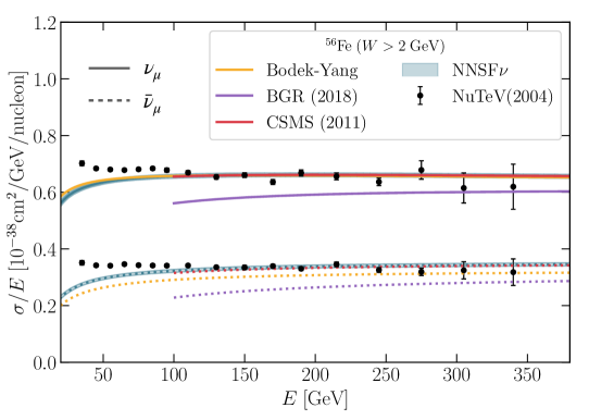
Figure 5.2: Same as the upper panel of Fig. 5.1, restricted to an iron target and focusing on the region between 20 GeV and 380 GeV. The predictions of NNSF$\nu$, Bodek-Yang, CSMS11 and BGR18 are compared with the experimental data from NuTeV [83] separately for neutrinos and antineutrinos. The invariant mass cut $W\geq 2$ GeV is applied to the theoretical calculations but not to the NuTeV measurement, explaining the disagreement for $E_{\nu}\mathrel{\hbox to0.0pt{\lower 4.0pt\hbox{\hskip 1.0pt$\sim$}\hss}\raise 1.0pt\hbox{$<$}}100$ GeV where other contributions in addition to inelastic scattering become significant.

For the energy region in which inelastic scattering dominates, $E_{\nu}\mathrel{\hbox to0.0pt{\lower 4.0pt\hbox{\hskip 1.0pt$\sim$}\hss}\raise 1.0pt\hbox{$>$}}100$ GeV, we find excellent agreement between the NuTeV data and the NNSF$\nu$ predictions, separately for neutrinos and antineutrinos. The Bodek-Yang calculation undershoots the NuTeV measurements on antineutrinos by up to 10%. CSMS11 is in good agreement with NNSF$\nu$ and the NuTeV data, while the BGR18 calculation, optimized for high-energy scattering, undershoots it for both neutrinos and antineutrinos. We note that the invariant mass cut $W\geq 2$ GeV is applied only to the theoretical calculations but not to the NuTeV measurement. This difference explains the disagreement for $E_{\nu}\mathrel{\hbox to0.0pt{\lower 4.0pt\hbox{\hskip 1.0pt$\sim$}\hss}\raise 1.0pt\hbox{$<$}}100$ GeV where other contributions in addition to inelastic scattering become significant, in particular resonant scattering. In this low-energy region, NNSF$\nu$ and Bodek-Yang exhibit the same qualitative behaviour.

Inelasticity.

In neutrino-hadron scattering, the inelasticity variable $y=Q^{2}/(2m_{N}xE_{\nu})$ represents the fraction of the incoming neutrino energy which is transferred to the hadronic final state and hence to the associated hadronic shower. The higher the value of $y$, the more energy that is transferred to the hadronic shower, facilitating the experimental measurement and characterisation of the latter. At intermediate energies, with $E_{\nu}\mathrel{\hbox to0.0pt{\lower 4.0pt\hbox{\hskip 1.0pt$\sim$}\hss}\raise 1.0pt\hbox{$<$}}100$ TeV, neutrino interactions are expected to produce on average more energetic hadronic showers than their antineutrino counterparts. Therefore, a measurement of the event-by-event inelasticity provides a useful handle in order to statistically separate $\nu$- from $\bar{\nu}$-bar initiated interactions, a feature exploited in the by IceCube analysis of [98]. The expected mean value of the inelasticity as a function of the neutrino energy can be computed as

$$\left\langle y\right\rangle(E_{\nu})=\left(\int_{Q^{2}_{\rm min}}^{Q^{2}_{\rm max}}{\rm d}Q^{2}\left[\int_{x_{0}(Q^{2})}^{1}{\rm d}x\,y\,{{{\rm d}^{2}\sigma^{\nu N}}\over{{\rm d}x{\rm d}Q^{2}}}(x,Q^{2},y)\right]\right)\Bigg{/}\sigma^{\nu N}(E_{\nu})\,,$$ (5.3)

using as input a given prediction for the double-differential scattering cross-section.

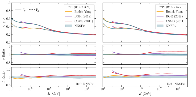
Figure 5.3: The mean value of the inelasticity, $\left\langle y\right\rangle$, relevant for inelastic neutrino scattering as a function of the neutrino energy $E_{\nu}$. The NNSF$\nu$ prediction, together with the associated 68% CL uncertainty band, is compared with the central values of the Bodek-Yang, BGR18, and CSMS11 calculations. The top panels displays the results for neutrinos and antineutrinos for both iron (left) and lead (right panel) targets, while the bottom ones display the ratios to the NNSF$\nu$ baseline separately for neutrino and antineutrino.

Fig. 5.3 displays the mean value of the inelasticity, Eq. (5.3), as a function of the neutrino energy for both iron and lead targets. The NNSF$\nu$ prediction for $\left\langle y\right\rangle$, together with the associated 68% CL uncertainty band, is compared with the central values of the Bodek-Yang, BGR18, and CSMS11 calculations. The bottom panels display the ratio of the different calculations with respect to the NNSF$\nu$ central value. As mentioned above, for $E_{\nu}\mathrel{\hbox to0.0pt{\lower 4.0pt\hbox{\hskip 1.0pt$\sim$}\hss}\raise 1.0pt\hbox{$<$}}100$ TeV the average inelasticity is markedly larger for neutrino-initiated scattering, while at higher energies the prediction for $\left\langle y\right\rangle$ becomes projectile-independent. An overall good agreement is observed between the different predictions, with differences up to the 10% level depending on the target and $E_{\nu}$ ranges. Specifically, at high neutrino energies, the NNSF$\nu$ prediction for $\left\langle y\right\rangle$ in a lead target is around 10% smaller as compared to CSMS11, partially explained by the nuclear corrections accounted for in the former but not in the latter. Good agreement between the Bodek-Yang and the NNSF$\nu$ calculations of $\left\langle y\right\rangle$ is obtained in the region of applicability of the former, with residual differences at the few percent level.

Sensitivity to the low-$Q$ region.

Fig. 5.4 displays the NNSF$\nu$ inclusive neutrino scattering cross-sections on an iron target for energies between 10 GeV and $10^{7}$ GeV, for different values of he lower integration limit $Q_{\rm min}$ in Eq. (5.1). Specifically, the default value of $Q_{\rm min}=0.03$ GeV is compared to calculations based on $Q_{\rm min}=$ 1, 1.41, and 2 GeV respectively. This comparison allows one to determine the relative contribution of the low-$Q$ region to the inclusive cross-sections as a function of $E_{\nu}$, an effect which is similar for neutrinos and antineutrinos.

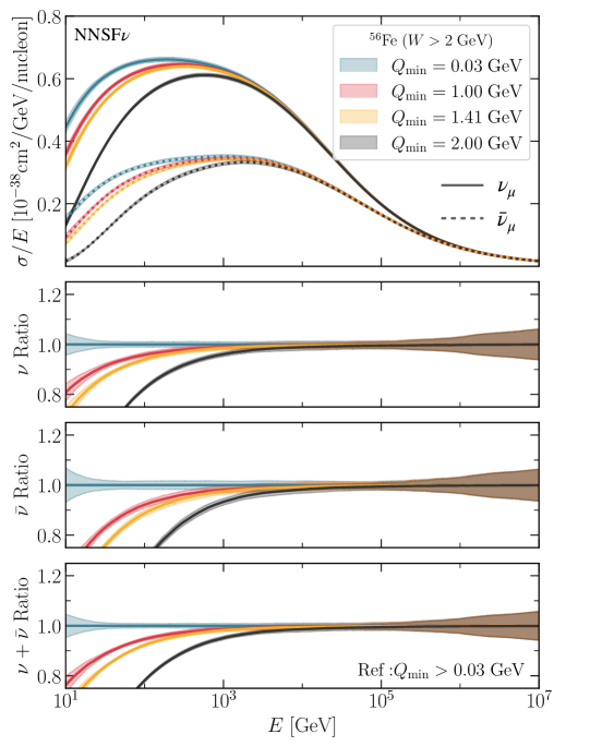
Figure 5.4: Same as Fig. 5.5 for an iron target and restricted to the energy region with $E_{\nu}\leq 10^{7}$ GeV. We assess the dependence of the inclusive cross-section with respect to variations in the lower integration limit $Q_{\rm min}$ in Eq. (5.1). The default value of $Q_{\rm min}=0.03$ GeV is compared to calculations based on $Q_{\rm min}=$ 1, 1.41, and 2 GeV.

From the analysis of Fig. 5.4 one determines that neutrinos with energies around $E_{\nu}\simeq 100$ GeV receive a contribution of up to 10% from the region with $Q\leq 1.41$ GeV and up to 25% from the region with $Q\leq 2$ GeV. As the neutrino energy is increased, the contribution from the low-$Q$ region decreases, but even for $E_{\nu}\approx 1$ TeV neutrinos, up to 10% of the inclusive cross-section can arise from momentum transfers of $Q\leq 2$ GeV. As discussed in Sect. 2, this low-$Q$ region is affected by sizable theory uncertainties (MHOUs, higher twists, mass effects, factorisation breakdown, ….), and hence Fig. 5.4 illustrates how the NNSF$\nu$ data-driven method makes it possible bypassing the limitations of the perturbative QCD calculation of neutrino inclusive cross-sections in the region $E_{\nu}\leq$ few TeV. It is interesting to highlight that for neutrino energies between 300 GeV and a few TeV, relevant for the interpretation of LHC far-forward neutrino scattering experiments, neither a data-driven, theory-agnostic calculation nor a purely QCD calculation can accurately predict the inclusive cross-sections. For higher neutrino energies, $E_{\nu}\mathrel{\hbox to0.0pt{\lower 4.0pt\hbox{\hskip 1.0pt$\sim$}\hss}\raise 1.0pt\hbox{$>$}}10$ TeV, the NNSF$\nu$ prediction becomes independent of structure functions in the $Q\leq 2$ GeV region and hence a perturbative QCD calculation of the cross-section such as that provided by YADISM can be reliably deployed.

5.2 Impact of nuclear effects

As illustrated by Fig. 5.1, the NNSF$\nu$ scattering cross section (per nucleon) on targets such as iron or lead is in general different to that evaluated on a isoscalar free-nucleon target. To further scrutinise the role that nuclear effects have on the inclusive neutrino cross-sections, Fig. 5.5 displays the NNSF$\nu$ predictions for the inelastic cross-section (divided by $E_{\nu}$) comparing the results of neutrino and antineutrino projectiles on deuterium (isoscalar free-nucleon), iron, and lead targets. The top panel displays the absolute cross-sections while the bottom ones show the ratio to the iron target baseline, sequentially for neutrinos, antineutrinos, and their sum. As in previous comparisons, the band in the NNSF$\nu$ predictions indicates the associated 68% CL uncertainties.

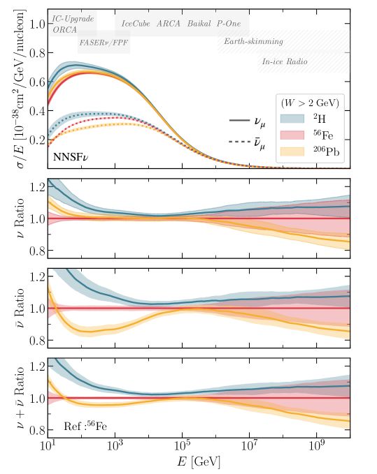
Figure 5.5: The NNSF$\nu$ predictions for the inclusive inelastic scattering cross-sections comparing the results of neutrino and antineutrino projectiles on deuterium, iron, and lead targets. The grey bands indicate the $E_{\nu}$ regions relevant for different experiments and detection techniques. The top panel displays the absolute cross-sections while the bottom ones the ratio to the iron target baseline sequentially for neutrinos, antineutrinos, and their sum.

To facilitate the identification of the different energy regions of interest for neutrino phenomenology, Fig. 5.5 also displays grey bands indicating the $E_{\nu}$ regions relevant for different experiments and detection techniques. Specifically, from low to high energies, we indicate the coverage of:

• $10\leavevmode\nobreak\ {\rm GeV}\mathrel{\hbox to0.0pt{\lower 4.0pt\hbox{\hskip 1.0pt$\sim$}\hss}\raise 1.0pt\hbox{$<$}}E_{\nu}\mathrel{\hbox to0.0pt{\lower 4.0pt\hbox{\hskip 1.0pt$\sim$}\hss}\raise 1.0pt\hbox{$<$}}300$ GeV: KM3NET-ORCA and DeepCore/IceCube-upgrade.

• $100\leavevmode\nobreak\ {\rm GeV}\mathrel{\hbox to0.0pt{\lower 4.0pt\hbox{\hskip 1.0pt$\sim$}\hss}\raise 1.0pt\hbox{$<$}}E_{\nu}\mathrel{\hbox to0.0pt{\lower 4.0pt\hbox{\hskip 1.0pt$\sim$}\hss}\raise 1.0pt\hbox{$<$}}4$ TeV: FASER$\nu$, SND@LHC, Forward Physics Facility (LHC far-forward neutrinos).

• $1\leavevmode\nobreak\ {\rm TeV}\mathrel{\hbox to0.0pt{\lower 4.0pt\hbox{\hskip 1.0pt$\sim$}\hss}\raise 1.0pt\hbox{$<$}}E_{\nu}\mathrel{\hbox to0.0pt{\lower 4.0pt\hbox{\hskip 1.0pt$\sim$}\hss}\raise 1.0pt\hbox{$<$}}10$ PeV: IceCube, KM3NET-ARCA, Baikal, P-One.

• $1\leavevmode\nobreak\ {\rm PeV}\mathrel{\hbox to0.0pt{\lower 4.0pt\hbox{\hskip 1.0pt$\sim$}\hss}\raise 1.0pt\hbox{$<$}}E_{\nu}\mathrel{\hbox to0.0pt{\lower 4.0pt\hbox{\hskip 1.0pt$\sim$}\hss}\raise 1.0pt\hbox{$<$}}10$ EeV: Earth-skimming neutrinos detection.

• $10\leavevmode\nobreak\ {\rm PeV}\mathrel{\hbox to0.0pt{\lower 4.0pt\hbox{\hskip 1.0pt$\sim$}\hss}\raise 1.0pt\hbox{$<$}}E_{\nu}\mathrel{\hbox to0.0pt{\lower 4.0pt\hbox{\hskip 1.0pt$\sim$}\hss}\raise 1.0pt\hbox{$<$}}10$ EeV: In-ice radio neutrino detection.

This list is not exhaustive, and has been added to the plot for illustrative purposes only.

As further discussed in App. C, two different types of nuclear effects are responsible for differences between scattering rates on a heavy nucleus and on a free proton (hydrogen target). The first is related to the different content in protons and neutrons, with iron (lead) containing $Z=26$ ($Z=82$) protons and $A-Z=30$ (126) neutrons. Therefore, as compared to a hydrogen target, the heavy nuclear targets display an enhanced (suppressed) content of down (up) valence quarks which leads in turn to an enhancement (suppression) of the associated structure functions for neutrino (antineutrino) scattering. This effect is most relevant in the valence structure function region, while as $E_{\nu}$ increases the cross section becomes dominated by small-$x$ scattering involving isospin-symmetric sea quarks and gluons. In the comparisons in Fig. 5.5 this effect is partially factored out since we normalise to an isoscalar ²H target, though the non-isoscalarity of heavy nuclei, specially in lead, still plays a role.

The second type of nuclear effect is the modifications of the structure of bound nucleons as compared to their free-nucleon counterparts. In the perturbative QCD region, these modifications are encoded by the nuclear PDFs, here taken from the nNNPDF3.0 determination. The corrections, quantified in App. C, are similar for neutrinos and antineutrinos and become most important in the shadowing region at medium and small-$x$, where a strong suppression in heavy nuclei is preferred. Nuclear structure modification effects are also present for $E_{\nu}\mathrel{\hbox to0.0pt{\lower 4.0pt\hbox{\hskip 1.0pt$\sim$}\hss}\raise 1.0pt\hbox{$<$}}1$ TeV, a region where they are partially described by the DIS calculations but which also receives contributions from the SIS region which cannot be expressed in terms of factorised nuclear PDFs. Within the NNSF$\nu$ framework, one estimates the nuclear modifications in Region I by allowing a free dependence of $F_{i}(x,Q^{2},A)$ to be directly constrained from the data, and then matched to the QCD calculation in Region II.

From the comparisons in Fig. 5.5, one observes that differences between inclusive cross-sections on Fe and Pb targets and those on ²H targets are moderate (a few percent at most) for energies in the intermediate region between 10 TeV and a few PeV. In the high energy region, for $E_{\nu}\mathrel{\hbox to0.0pt{\lower 4.0pt\hbox{\hskip 1.0pt$\sim$}\hss}\raise 1.0pt\hbox{$>$}}10$ TeV, the most marked effect is the strong suppression of the cross-sections in lead as compared to those in a free-nucleon target, reaching up to 20% at 100 EeV. This suppression is a consequence of the small-$x$ shadowing of quark and gluons in nNNPDF3.0. Given the large nPDF uncertainties associated to an iron target, high-energy cross-sections for Fe are compatible within errors with those for both ²H and Pb.

In the region where the non-DIS contribution is sizable, $E_{\nu}\mathrel{\hbox to0.0pt{\lower 4.0pt\hbox{\hskip 1.0pt$\sim$}\hss}\raise 1.0pt\hbox{$<$}}1$ TeV, differences between Fe and Pb targets for the $\nu+\bar{\nu}$ cross-section remain at the few percent level, with again the latter being suppressed in comparison to the former. The cross-sections on a ²H target are enhanced at low energies, with the difference being up to 20% in the $E_{\nu}=10$ GeV where the inelastic component is very small. In the same energy region, differences between the three nuclear targets appear to be less (more) significant once we consider separately the predictions for neutrinos (antineutrinos).

While in this section we discuss explicitely nuclear effects only for Pb and Fe targets, NNSF$\nu$ structure functions and inclusive cross-section predictions are provided for all targets relevant for neutrino phenomenology and summarised in Table A.1. In addition, below we provide dedicated predictions for the energy ranges and target materials relevant for far-forward neutrino experiments at the LHC.

5.3 Far-forward neutrino scattering at the LHC

Precise predictions for neutrino scattering rates are a key ingredient for the interpretation of data from experiments aiming to detect and study the far-forward neutrinos produced in LHC collisions. These include the current SND@LHC and FASER$\nu$ experiments as well as the proposed AdvSND@LHC, FLArE, and FASER$\nu$2, which would be installed in the Forward Physics Facility operating concurrently with the HL-LHC. The dominant component of these far-forward LHC neutrino fluxes lies in the region between a few hundreds of GeV and a few TeV [99, 100], with the high-energy component most sensitive to neutrinos produced from charm meson decays. Here we provide dedicated predictions for the inclusive neutrino scattering cross-sections in the FPF energy range, specifically between $E_{\nu}=100$ GeV and 10 TeV, assuming a tungsten (W) nuclear target with $A=184$, which is the current target of FASER$\nu$ and the intended target for the FASER$\nu$2 experiment. For completeness, we also provide predictions for neutrino scattering on an oxygen (O) target, which are relevant for the intepretation of ongoing and future neutrino oscillation measurements taking place at the DeepCore/IceCube and KM3NET-ORCA experiments in a partially overlapping energy range as the FPF.

With this motivation, Fig. 5.6 (left) presents the same comparison as in Fig. 5.1 now on a tungsten target and restricted to the energy region relevant for the FPF experiments. In this energy region and for this specific nuclear target, one observes excellent agreement between the NNSF$\nu$ determination and the Bodek-Yang model predictions, except perhaps for antineutrinos with $E_{\nu}$ of several TeV. Given that the two calculations are completely different in terms of both data and QCD input as well as in methodological assumptions, such agreement at the $1\%$ level is remarkable. The CSMS11 (BGR18) predictions tend to overestimate (underestimate) the FPF neutrino scattering rates in comparison to the NNSF$\nu$ baseline, specially for BGR18 at low energies where the calculation falls outside its regime of applicability.

Figure 5.6: Left: same as Fig. 5.1 on a tungsten (W) target and restricted to the energy region relevant for the FPF experiments. Right: same as Fig. 5.5 comparing the NNSF$\nu$ predictions for W and O targets, again in the range covered by neutrino scattering at the FPF.

All in all, Fig. 5.6 demonstrates that the uncertainties on the inclusive neutrino cross-section predictions for a W target at FPF energies are estimated to be at most at the 5% level, and even less for the combined $\nu+\bar{\nu}$ cross-section. We conclude that state-of-the-art calculations of neutrino scattering in the SM at the FPF energies can achieve a precision of a few percent, thus providing an excellent starting point for further investigations of neutrino interactions in this unexplored energy range, for instance in terms of anomalous couplings or of EFT effects.

The right panel of Fig. 5.6 displays a similar comparison as that of Fig. 5.5, now for the NNSF$\nu$ predictions for tungsten and oxygen targets. While neutrino cross-sections display almost no differences between the two targets, for the antineutrino case we observe sizable nuclear effects, of up to 20% and specially for energies below 1 TeV. As the energy is increased, the differences related to nuclear corrections wash away but even at 10 TeV they can represent a 10% effect. The predictions for the combined $\nu+\bar{\nu}$ cross-section, averaged over the two projectiles, lead to more moderate differences but still up to the 10% level at energies of few hundreds of GeV. Fig. 5.6 indicates that properly accounting for nuclear effects associated to the target material is required in order to translate constraints on neutrino interactions obtained from the FPF experiments to those from KM3NET and IceCube analyses and vice-versa, specially in those cases where one is sensitive to the separation between neutrinos and antineutrinos in the initial state.

6 Summary and outlook

We have presented a novel approach to the determination of neutrino inelastic structure functions based on the combination of a data-driven parametrisation at low and moderates values of $Q^{2}$ matched to perturbative QCD calculations at high $Q^{2}$. The resulting structure functions, dubbed NNSF$\nu$, enable the evaluation of inclusive neutrino scattering cross sections over 12 orders of magnitude in energy $E_{\nu}$ from a few GeV up to the multi-EeV region. In particular, it makes possible the accurate evaluation of scattering event rates for neutrinos with energies between 100 GeV and a few TeV, relevant for both far-forward neutrino detection at the LHC and for atmospheric neutrino oscillation experiments, without the need to impose acceptance cuts in $Q^{2}$. The NNSF$\nu$ determination comes accompanied with a faithful estimate of the associated uncertainties and accounts for the constraints provided by state-of-the-art determinations of nucleon and nuclear structure.

We have compared the NNSF$\nu$ determination with existing calculations in the literature, such as the popular Bodek-Yang model, both at the level of structure functions and of inclusive cross sections. We have demonstrated the agreement between our parametrisation and the experimental data, highlighted the smooth matching between the data-driven extraction and the QCD boundary conditions, and assessed the behaviour of NNSF$\nu$ in the extrapolation regions. We have quantified the impact of nuclear PDF modifications, finding that these are most significant for heavy nuclei such as tungsten and lead. We have also studied the implications of the NNSF$\nu$ analysis for key observables in neutrino DIS, such as the Gross-Llewellyn-Smith sum rule.

The NNSF$\nu$ determination is made available in terms of LHAPDF interpolation tables [66] for neutrino structure functions corresponding to the relevant nuclear targets, as described in App. A. Two different sets of grids are provided, one associated to the neural network determination and the other to the YADISM calculation, and a Python script showcasing how to use and combine these two grids is provided. We also provide a script that takes as input these LHAPDF structure function grids and integrates them to evaluate the inclusive cross section and the corresponding uncertainties. For completeness, we also make available look-up tables with the NNSF$\nu$ predictions for inclusive cross sections $\sigma^{\nu A}(E_{\nu})$ in the relevant range of $E_{\nu}$ and target nuclei. The LHAPDF grids, Python driver scripts, and look-up tables are available from the project GitHub repository

https://nnpdf.github.io/nnusf

together with the data, code, and theory tables that enter the structure function determination. The NNSF$\nu$ structure functions have also been implemented in the GENIE [20] event generator, where it can be accessed in a similar manner as the BGR18 and Bodek-Yang calculations. It is hence readily available in a software framework already integrated in the analysis pipeline of many neutrino experiments.

The results presented in this work could be expanded in different directions. First, far-forward neutrino measurements taking place at LHC experiments such as FASER$\nu$ and SND@LHC, and in the longer term the Forward Physics Facility, will provide further constraints on the modelling of neutrino scattering at low and moderate $Q^{2}$. Second, the NNSF$\nu$ calculation could be integrated into other neutrino event generators to streamline its usage, also for neutrino experiments where inelastic scattering, without dominating, still represents a sizable contribution to the total event rates. Third, by incorporating updated determinations of proton and nuclear PDFs benefitting from new experimental constraints and higher-order theory calculations, such as the information provided by charm production at LHCb combined with small-$x$ BFKL resummation to improve predictions of neutrino structure functions at UHE energies [71, 40, 41]. Fourth, by considering the information provided by lattice QCD calculations [101] to constrain structure functions in the non-perturbative low $Q^{2}$ region.

All in all, the NNSF$\nu$ analysis bridges a significant gap in current neutrino phenomenology by providing a consistent determination of structure functions enabling the calculation of cross sections in the full range of $E_{\nu}$ relevant for inelastic scattering. For the first time, a determination of structure functions can be used for predictions involving accelerator neutrinos with $E_{\nu}\sim{\rm few\leavevmode\nobreak\ GeV}$, atmospheric and collider neutrinos with energies between $\sim{\rm 100\leavevmode\nobreak\ GeV}$ and ${\rm few\leavevmode\nobreak\ TeV}$, and ultra-high energy neutrino scattering at EeV energies. The availability of NNSF$\nu$ allows bypassing a major limitation of current analyses where different cross-section calculations, inconsistent among them, have to be adopted depending on the range of energies involved.

Acknowledgments

We thank Jonathan Feng, Felix Klein, Hallsie Reno, and Dennis Soldin for productive discussions concerning neutrino scattering in the context of the Forward Physics Facility working group. We are grateful to Nusch Mortazavi for collaborations in an early stage of the project. A. C. and partially R. S. are supported by the European Research Council under the European Union’s Horizon 2020 research and innovation Programme (grant agreement n.740006). R. S. is partially supported by the U.K. Science and Technology Facility Council (STFC) grant ST/P000630/1. J. R. and G. M. are partially supported by NWO (Dutch Research Council). J. R. and T. R. are supported by an ASDI (Accelerating Scientific Discoveries) grant from the Netherlands eScience Center. A. G. acknowledges support from the European Union’s H2020-MSCA Grant Agreement No.101025085 and the Faculty of Arts and Sciences of Harvard University.

Appendix A Usage and delivery of the NNSF$\nu$ determination

The software framework used to produce the NNSF$\nu$ determination of neutrino inelastic structure functions, together with the results obtained from it, can be obtained from the project website:

https://nnpdf.github.io/nnusf

Specifically, there one can find the following:

• Installation instructions, code documentation, and user-friendly examples of the NNSF$\nu$ software framework, including the data and theory runcards that allow reproducing the results of this paper.

• Fast interpolation grids in $x$ and $Q^{2}$ for the inelastic structure functions $F_{2}$, $xF_{3}$, and $F_{L}$ for neutrinos, antineutrinos, and their sum. These structure function grids can be accessed by means of the LHAPDF interface and are provided for all nuclear targets of phenomenological relevance for neutrino scattering experiments.

• A driver code that evaluates, taking these structure functions grids as inputs, the corresponding central values, uncertainties, and correlations. As explained below, two structure function parametrisations with a different coverage in the $(x,Q^{2})$ plane are provided and the driver code takes care of their combination.

• A second Python driver code that evaluates the inclusive neutrino cross section Eq. (5.1) as a function of $E_{\nu}$ from the LHAPDF grids and provides the corresponding uncertainty estimate.

• Look-up tables compiling the NNSF$\nu$ predictions for the inclusive cross sections $\sigma^{\nu A}$ and $\sigma^{\bar{\nu}A}$ for phenomenologically relevant nuclei as a function of $E_{\nu}$, together with their uncertainty estimates.

In this appendix we provide details on these deliveries associated to the NNSF$\nu$ determination, from the code and documentation to the inclusive cross-section look-up tables. In particular, we describe the prescriptions required to evaluate central values and uncertainties for the structure functions and inclusive cross sections from the LHAPDF grids provided.

The NNSF$\nu$ framework.

The framework developed in this work provides a stand-alone code to parametrise structure functions from experimental data in the presence of general theory constraints. It provides an independent implementation of the NNPDF fitting methodology, and shares the main methodological aspects with the NNPDF4.0 and nNNPDF3.0 proton and nuclear PDF determination such as the use of Stochastic Gradient Descent for the minimisation. For the first time in this context, neural networks with three independent inputs $(x,Q^{2},A)$ are used to parametrise unknown functions from experimental data.

Structure functions.

Table A.1 lists the NNSF$\nu$ structure function grids released in the LHAPDF format. We indicate the values of $(Z,A)$ for each nuclear target and the names of the corresponding low-$Q$ and high-$Q$ grids. Each grid provides, as a function of $x$ and $Q^{2}$, as outputs the neutrino and antineutrino structure functions as well as their sum, namely

$$F_{2}^{\nu A}(x,Q^{2})\,,F_{L}^{\nu A}(x,Q^{2})\,,xF_{3}^{\nu A}(x,Q^{2})\,,$$

$$F_{2}^{\bar{\nu}A}(x,Q^{2})\,,F_{L}^{\bar{\nu}A}(x,Q^{2})\,,xF_{3}^{\bar{\nu}A}(x,Q^{2})\,,$$ (A.1)

$$F_{2}^{(\nu+\bar{\nu})A}(x,Q^{2})\,,F_{L}^{(\nu+\bar{\nu})A}(x,Q^{2})\,,xF_{3}^{(\nu+\bar{\nu})A}(x,Q^{2})\,,$$

with the PDG ID codes being respectively [1001, 1002, 1003, 2001, 2002, 2003, 3001, 3002, 3003]. We emphasize that the number of replicas, coverage on $x$ and $Q^{2}$, and statistical interpretation of the low- and high-$Q$ grids is different, as discussed below. The nuclear targets listed in Table A.1 are selected for their relevance in the interpretation of past and present experimental data as well for theoretical predictions for upcoming experiments. For instance, tungsten (W) is relevant for the event rate predictions at FASER$\nu$ and its eventual successor FASER$\nu$2, while oxygen (O) enters scattering rates for neutrinos on air, water, or ice targets. We also provide a grid for $(A,Z)=(15,31)$, which correspond to the average nuclear numbers for Earth matter relevant for calculations of UHE neutrino attenuation when crossing the Earth [22].

$(Z,A)$ [target]	low-$Q$ grid	high-$Q$ grid
$(1,2)$ [D]	NNSFnu_D_lowQ	NNSFnu_D_highQ
$(2,4)$ [He]	NNSFnu_He_lowQ	NNSFnu_He_highQ
$(3,6)$ [Li]	NNSFnu_Li_lowQ	NNSFnu_Li_highQ
$(4,9)$ [Be]	NNSFnu_Be_lowQ	NNSFnu_Be_highQ
$(6,12)$ [C]	NNSFnu_C_lowQ	NNSFnu_C_highQ
$(7,14)$ [N]	NNSFnu_N_lowQ	NNSFnu_N_highQ
$(8,16)$ [O]	NNSFnu_O_lowQ	NNSFnu_O_highQ
$(13,27)$ [Al]	NNSFnu_Al_lowQ	NNSFnu_Al_highQ
$(15,31)$ [Ea]	NNSFnu_Ea_lowQ	NNSFnu_Ea_highQ
$(18,39)$ [Ar]	NNSFnu_Ar_lowQ	NNSFnu_Ar_highQ
$(20,40)$ [Ca]	NNSFnu_Ca_lowQ	NNSFnu_Ca_highQ
$(26,56)$ [Fe]	NNSFnu_Fe_lowQ	NNSFnu_Fe_highQ
$(29,64)$ [Cu]	NNSFnu_Cu_lowQ	NNSFnu_Cu_highQ
$(47,108)$ [Ag]	NNSFnu_Ag_lowQ	NNSFnu_Ag_highQ
$(50,119)$ [Sn]	NNSFnu_Sn_lowQ	NNSFnu_Sn_highQ
$(54,131)$ [Xe]	NNSFnu_Xe_lowQ	NNSFnu_Xe_highQ
$(74,184)$ [W]	NNSFnu_W_lowQ	NNSFnu_W_highQ
$(79,197)$ [Au]	NNSFnu_Au_lowQ	NNSFnu_Au_highQ
$(82,208)$ [Pb]	NNSFnu_Pb_lowQ	NNSFnu_Pb_highQ

Table A.1: The NNSF$\nu$ structure function grids released in the LHAPDF format. We indicate the values of $(Z,A)$ for each nuclear target and the names of the corresponding low-$Q$ and high-$Q$ grids. Each grid provides, as a function of $x$ and $Q^{2}$, as outputs the neutrino and antineutrino structure functions $F_{2}$, $xF_{3}$, and $F_{L}$ as well as their sum. We note that both the number of replicas and the statistical interpretation thereof is different in the low- and high-$Q$ grids, see text for more details.

The low-$Q$ and high-$Q$ NNSF$\nu$ structure function grids are defined as follows:

• low-$Q$ grid. This grid encapsulates the direct output of the NNSF$\nu$ neural networks trained on the neutrino structure function data and supplemented by the theoretical constraints from the QCD calculation based on nNNPDF3.0.

  The LHAPDF grid is constituted by a central set and $N_{\rm rep}=200$ Monte Carlo replicas, which represent the probability density in the space of fitted structure functions and from which statistical estimators such CL intervals can are evaluated with the usual NNPDF prescription. The central set is defined as the average over the $N_{\rm rep}$ replicas. The uncertainty band associated with these replicas receives two contributions: the experimental uncertainties associated to the input fitted neutrino data and those associated to the methodology such as the functional uncertainty, in both cases subject to the constraints provided by the QCD boundary conditions imposed during the fit.

  This low-$Q$ grid can be used in the kinematic region

  $$0.01\leavevmode\nobreak\ {\rm GeV}\leq Q\leq 22\leavevmode\nobreak\ {\rm GeV}\,\quad{\rm and}\quad 10^{-5}\leq x\leq 1\,.$$ (A.2)

  We note that extending this coverage could be achieved by enlarging the $(x,Q^{2})$ coverage of the QCD constraints added to the fit, but this may distort the fit quality by decreasing the weight given to the experimental data. If values of $(x,Q^{2})$ outside the region defined by Eq. (A.2) are requested, the output will be determined by the LHAPDF extrapolation algorithm.

• high-$Q$ grid. This grid tabulates the direct output of the YADISM calculation of neutrino structure functions at NLO in QCD with nNNPDF3.0 together with the corresponding uncertainties. This calculation is independent of the output of the neural network parametrisation used for the low-$Q$ grid, though the respective central values are matched due to their use of the same QCD calculation.

  The LHAPDF grid is constituted by a central set, $\widetilde{N}_{\rm rep}=200$ replicas that correspond to the nNNPDF3.0 replicas and structure functions obtained with central factorisation and renormalisation scales, $\mu_{F}=\mu_{R}=1$, and 9 additional “replicas” computed with the central nNNPDF3.0 set and with nine $\mu_{R}$ and $\mu_{F}$ scale variations following the procedure outlined in Sect. 3. The central set in this grid is evaluated as the average of the $\widetilde{N}_{\rm rep}=200$ replicas. Therefore this grid is constituted by 210 members (including the central predictions). PDF uncertainties and MHOUs can be obtained and combined by means of the procedure from [93], where the latter are obtained with the 9-point prescription and then added in quadrature with the PDF uncertainties. The scripts delivered with the grids illustrate how the uncertainty calculation is carried out.

  This high-$Q$ grid can be used in the kinematic region

  $$2\leavevmode\nobreak\ {\rm GeV}\leq Q\leq 10\leavevmode\nobreak\ {\rm TeV}\,\quad{\rm and}\quad 10^{-9}\leq x\leq 1\,,$$ (A.3)

  and again outside this region the grid output is obtained from LHAPDF extrapolation. Restricting the YADISM calculation to this region ensures the validity of the pQCD calculation.

  We note that Eqns. (A.2) and (A.3) overlap in the region of $(x,Q^{2})$ where both the data-driven and pQCD approaches can be reliably applied. In this overlap region, we recommend using the outcome of the low-$Q$ grid as baseline.

• Grid matching. Within their respective regions of applicability, one can evaluate the neutrino structure functions and the associated uncertainties using the appropriate prescription. If we denote by $F^{\nu A}_{i,lQ}(x,Q^{2})$ and $F^{\nu A}_{i,hQ}(x,Q^{2})$ the outcome of the $F_{i}$ structure function obtained from the low-$Q$ and high-$Q$ grids respectively, to evaluate the neutrino structure function one should use the prescription:

  $$F_{i}^{\nu A}(x,Q^{2})=\begin{cases}F^{\nu A}_{i,lQ}(x,Q^{2}),&\text{if}\ Q\leq Q_{\rm thr}\,\,\&\,\,x\geq 10^{-3}\,,\\[8.5359pt] F^{\nu A}_{i,hQ}(x,Q^{2}),&\text{otherwise}\,,\end{cases}$$ (A.4)

  with $Q_{\rm thr}=22$ GeV, and the same holds for the corresponding uncertainties. We emphasize that the replicas of the low-$Q$ grids can be treated as correlated among them, and the same holds for those of the low-$Q$ grids, but that replicas of the low-$Q$ grid are uncorrelated with those of the high-$Q$ grid. The user can vary the matching parameters in Eq. (A.4), for instance by choosing a lower $Q^{2}$ threshold $Q_{\rm thr}$ to switch to the high-$Q$ grid calculation.

  Since the same pQCD calculation that is tabulated in $F^{\nu A}_{i,hQ}$ enters the data-driven fit of $F^{\nu A}_{l,hQ}$ as theoretical constraint, central values obtained from the prescription of Eq. (A.4) should match within uncertainties as one crosses the threshold value $Q_{\rm thr}$. This does not necessarily hold for the structure function uncertainties, since these are typically larger in the data-driven fit than in the pQCD calculation. If required, the user may implement the matching of the structure function uncertainty across the threshold $Q_{\rm thr}$ by means of a sliding window prescription.

As mentioned above, in the project website we provide a Python code that evaluates neutrino structure functions and their uncertainties for any value of $x$ and $Q^{2}$ following the prescription outlined above.

Neutrino inclusive cross sections.

Inclusive neutrino structure functions are evaluated by integrating the output of the structure function grids described above using Eq. (5.1). As highlighted by the analysis of Sect. 5.1, for neutrino energies of $E_{\nu}\mathrel{\hbox to0.0pt{\lower 4.0pt\hbox{\hskip 1.0pt$\sim$}\hss}\raise 1.0pt\hbox{$>$}}10$ TeV the contribution from the kinematic region involving $Q\mathrel{\hbox to0.0pt{\lower 4.0pt\hbox{\hskip 1.0pt$\sim$}\hss}\raise 1.0pt\hbox{$<$}}2$ GeV is negligible, and in such case one can evaluate the cross section in terms of only the high-$Q$ structure function grid. Conversely, for lower neutrino energies, say $E_{\nu}\mathrel{\hbox to0.0pt{\lower 4.0pt\hbox{\hskip 1.0pt$\sim$}\hss}\raise 1.0pt\hbox{$<$}}100$ GeV, the integral in Eq. (5.1) will be dominated by momentum transfers with $Q\mathrel{\hbox to0.0pt{\lower 4.0pt\hbox{\hskip 1.0pt$\sim$}\hss}\raise 1.0pt\hbox{$<$}}20$ GeV and hence it can be evaluated in terms of entirely the output of the low-$Q$ structure function grid. For intermediate values of the neutrino energy, one can combines the low- and high-$Q$ structure function grid.

To further illustrate the kinematic coverage of the integrated neutrino cross-section calculation, Fig. A.1 displays the coverage in the $(x,Q^{2})$ plane of the inclusive cross section Eq. (5.1) in muon-neutrino inelastic scattering. We consider three values of the neutrino energy: from left to right, $E_{\nu}=11$ GeV, 90 TeV, and 1 EeV. The blue bins indicate the regions in $(x,Q^{2})$ that contribute to the inclusive cross-section (normalised to the maximum value of the integrand), with darker bins dominating the integral. The region covered by red (green) indicates that the output of low-$Q$ (high-$Q$) structure function grid is being used to evaluate the inclusive cross section. For $E_{\nu}=11$ GeV, the cross section is determined entirely by the output of the low-$Q$ grid. For $E_{\nu}=90$ TeV, the output of the two grids are required, carrying a similar weight in the calculation. For $E_{\nu}=1$ EeV, the cross section depends only on perturbative structure functions and the bulk of the contribution is associated to the region around $x\simeq 10^{-5}$ and $Q\simeq 100$ GeV. From this last case, one can see how at high neutrino energies it is important to also account for the region with $x\mathrel{\hbox to0.0pt{\lower 4.0pt\hbox{\hskip 1.0pt$\sim$}\hss}\raise 1.0pt\hbox{$<$}}10^{-5}$ and $Q\mathrel{\hbox to0.0pt{\lower 4.0pt\hbox{\hskip 1.0pt$\sim$}\hss}\raise 1.0pt\hbox{$<$}}Q_{\rm thr}$, which is covered by the high-$Q$ grid but not by the low-$Q$ one.

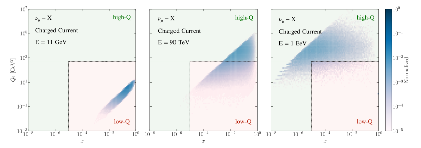
Figure A.1: The coverage in the $(x,Q^{2})$ plane of the inclusive neutrino cross section, Eq. (5.1), in muon-neutrino inelastic scattering. We consider three values of the neutrino energy: from left to right, $E_{\nu}=11$ GeV, 90 TeV, and 1 EeV. The blue bins indicate the regions in $(x,Q^{2})$ that contribute to the inclusive cross-section (normalised to the maximum value of the integrand), with darker bins dominating the integral. The region covered by red (green) indicates that the output of low-$Q$ (high-$Q$) structure function grid is being used to evaluate the inclusive cross section, see text for more details.

Taking into account the contribution from the relevant kinematics, the integration is Eq. (5.1) is separated into three disjoint regions

$$\sigma^{\nu N}(E_{\nu})=\int_{0}^{Q^{2}_{\rm max}}{\rm d}Q^{2}\left[\int_{x_{0}(Q^{2})}^{1}{\rm d}x{{{\rm d}^{2}\sigma^{\nu N}}\over{{\rm d}x{\rm d}Q^{2}}}(x,Q^{2},y)\right]=\sigma^{\nu N}_{lQ}(E_{\nu})+\sigma^{\nu N}_{hQ}(E_{\nu})\equiv\qquad$$

$$\int_{0}^{Q^{2}_{\rm thr}}{\rm d}Q^{2}\left[\int_{{\rm max}\left(x_{0}(Q^{2}),10^{-5}\right)}^{1}{\rm d}x{{{\rm d}^{2}\sigma_{lQ}^{\nu N}}\over{{\rm d}x{\rm d}Q^{2}}}(x,Q^{2},y)\right]+\int_{Q^{2}_{\rm thr}}^{Q^{2}_{\rm max}}{\rm d}Q^{2}\left[\int_{x_{0}(Q^{2})}^{1}{\rm d}x{{{\rm d}^{2}\sigma_{hQ}^{\nu N}}\over{{\rm d}x{\rm d}Q^{2}}}(x,Q^{2},y)\right]$$ (A.5)

$$+\int_{Q^{2}_{\rm min}}^{Q^{2}_{\rm thr}}{\rm d}Q^{2}\left[\int_{{\rm min}\left(x_{0}(Q^{2}),10^{-5}\right)}^{1}{\rm d}x{{{\rm d}^{2}\sigma_{hQ}^{\nu N}}\over{{\rm d}x{\rm d}Q^{2}}}(x,Q^{2},y)\right]\,,\qquad\qquad\qquad$$

separated by the threshold $Q^{2}_{\rm thr}$, in terms of structure functions computed with low- and high-$Q$ grids, in analogy with Eq. (A.4), and with $Q^{2}_{\rm min}=1.65$ GeV to ensure that the high-$Q$ grid is not extrapolated to the non-perturbative region. Depending on the $E_{\nu}$ value, one we can simplify Eq. (A) to

$$\sigma^{\nu N}(E_{\nu})=\begin{cases}\simeq\sigma^{\nu N}_{lQ}(E_{\nu})&\text{if}\,E_{\nu}\mathrel{\hbox to0.0pt{\lower 4.0pt\hbox{\hskip 1.0pt$\sim$}\hss}\raise 1.0pt\hbox{$<$}}1\leavevmode\nobreak\ {\rm TeV}\,,\\[8.5359pt] \simeq\sigma^{\nu N}_{hQ}(E_{\nu})&\text{if}\,E_{\nu}\mathrel{\hbox to0.0pt{\lower 4.0pt\hbox{\hskip 1.0pt$\sim$}\hss}\raise 1.0pt\hbox{$>$}}100\leavevmode\nobreak\ {\rm PeV}\,,\\[8.5359pt] \sigma^{\nu N}_{lQ}(E_{\nu})+\sigma^{\nu N}_{hQ}(E_{\nu})\quad&\text{otherwise}\,,\end{cases}$$ (A.6)

since at low and high energies only the low-$Q$ and high-$Q$ structure function grids are required respectively, with the other term leading to a negligible contribution. We note that, as also indicated by Fig. A.1, at high neutrino energies the high-$Q$ grid is also used for $Q\mathrel{\hbox to0.0pt{\lower 4.0pt\hbox{\hskip 1.0pt$\sim$}\hss}\raise 1.0pt\hbox{$<$}}Q_{\rm thr}$ to determine the contribution for $x\leq 10^{-5}$ which is not covered by the low-$Q$ grid.

Given the different statistical interpretation of the uncertainties associated to the low- and high-$Q$ structure function grids, the total uncertainty in Eq. (A) is evaluated by adding in quadrature the uncertainties associated to the low- and high-$Q$ contributions, namely

$$\delta\sigma^{\nu N}(E_{\nu})=\left(\left(\delta\sigma^{\nu N}_{lQ}(E_{\nu})\right)^{2}+\left(\delta\sigma^{\nu N}_{hQ}(E_{\nu})\right)^{2}\right)^{1/2}\,,$$ (A.7)

with $\delta\sigma^{\nu N}_{lQ}$ and $\delta\sigma^{\nu N}_{hQ}$ evaluated using the uncertainty prescription for the low- and high-$Q$ structure function grids respectively. As opposed to the structure function case, the prescriptions Eq. (A), for central values, and (A.7), for the total uncertainties, lead to smooth predictions for neutrino energies $E_{\nu}$ sensitive both to low- and high-$Q$ structure functions. Furthermore, the outcome of the cross-section calculation is stable upon moderate variations of the threshold value $Q^{2}_{\rm thr}$.

The matching procedure described in this appendix to evaluate inclusive neutrino cross sections in terms of the NNSF$\nu$ structure functions by means of the prescriptions of Eq. (A), for central values, and Eq. (A.7), for the total uncertainties, is illustrated in Fig. A.2. The NNSF$\nu$ predictions of the inclusive cross sections for neutrino and antineutrino scattering off an iron target are compared to the corresponding individual contributions from the low-$Q$ and high-$Q$ structure function grids, denoted by $\sigma^{\nu N}_{lQ}(E_{\nu})$ and $\sigma^{\nu N}_{hQ}(E_{\nu})$ respectively in Eq. (A). For low ($E_{\nu}\mathrel{\hbox to0.0pt{\lower 4.0pt\hbox{\hskip 1.0pt$\sim$}\hss}\raise 1.0pt\hbox{$<$}}1$ TeV) and high ($E_{\nu}\mathrel{\hbox to0.0pt{\lower 4.0pt\hbox{\hskip 1.0pt$\sim$}\hss}\raise 1.0pt\hbox{$>$}}100$ PeV) values of the neutrino energy, the calculation is fully dominated by the contributions from the low- and high-$Q$ structure function grids respectively, as indicated by Eq. (A.6), while for intermediate $E_{\nu}$ values between 1 TeV and 100 PeV one must account for both contributions. It is worthwhile noting that the contribution from the low-$Q$ grid remains relevant up to rather high neutrino energies. The smooth dependence in $E_{\nu}$ both for central values and uncertainties further validates the NNSF$\nu$ matching which connects the various energy regions.

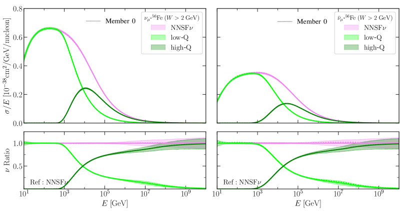
Figure A.2: The NNSF$\nu$ predictions for inclusive cross sections for neutrino (left) and antineutrino (right panel) scattering off an iron target. We indicate the individual contributions from the low-$Q$ and high-$Q$ structure function grids, denoted by $\sigma^{\nu N}_{lQ}(E_{\nu})$ and $\sigma^{\nu N}_{hQ}(E_{\nu})$ respectively in Eq. (A), as well as their sum that defines the NNSF$\nu$ prediction. The NNSF$\nu$ uncertainty is evaluated by adding in quadrature the (uncorrelated) contribution from the two grids as indicated by Eq. (A.7). The bottom panels display the results normalised to the central value of NNSF$\nu$.

Appendix B YADISM: DIS structure functions made easy

Deep-inelastic structure functions can be evaluated with several public codes such as APFEL [69] and QCDNUM [102]. Available DIS codes differ in the accuracy with which structure functions can be computed, whether they are based on the $x$-space or the $N$-space formalism, the treatment of heavy quark mass effects and of target mass corrections, the availability of polarised and time-like coefficient functions, and the possible inclusion of QED corrections among other considerations.

This appendix introduces YADISM, a new framework for the evaluation of DIS structure functions from the same family as the EKO [64] DGLAP evolution code. The open source YADISM code can be obtained from its GitHub repository

https://github.com/NNPDF/yadism/

together with an detailed documentation, tutorials, and user-friendly examples

https://yadism.readthedocs.io/

One of the main advantages of YADISM is that it is integrated with the fast interpolation grid toolbox PineAPPL [103], and hence DIS structure functions can be treated on the same footing as hadronic observables from the point of view of PDF fitting and related applications. PineAPPL provides a unique grid format, with application programming interfaces (APIs) for different programming languages and a command-line interface to manage the grid files. Furthermore, YADISM implements the available N³LO DIS coefficient functions, which combined with (approximate) N³LO evolution and heavy quark matching conditions available in EKO provide theoretical calculations required to carry out a N³LO PDF determination. YADISM will be described in an upcoming publication [104], here we summarise its main features, in particular those relevant to the present study, and highlight benchmarking studies carried out.

Grid formalism.

As indicated by Eq. (2.9), in the perturbative regime DIS structure functions are given by the factorised convolution of process-dependent partonic scattering cross sections and of process-independent parton distribution functions,

$$F_{i}(x,Q^{2})=\sum_{j}\int_{x}^{1}{{dz}\over{z}}\,C_{i,j}(z,\alpha_{s}(Q^{2}))f_{j}\left({{x}\over{z}},Q^{2}\right)\equiv C_{j;i}\otimes f_{j}\,,$$ (B.1)

where $j$ is an index that runs over all possible partonic initial states and $C_{i,j}$ is the process-dependent, but target-independent, coefficient function, given by an expansion in the QCD coupling $\alpha_{s}(Q^{2})$. In the third term of Eq. (B.1) and in the following, sum over repeated indices is implicit.

As standard for fast interpolation techniques developed in the context of PDF fits [105, 103, 106, 107], the PDFs can be expanded over an interpolation basis

$$f_{j}(\xi)=\sum_{\alpha}p_{\alpha}(\xi)f(\xi_{\alpha})\equiv p_{\alpha}(\xi)f_{\alpha}\,,\qquad\xi={{x}\over{z}}\,,$$ (B.2)

with $p_{\alpha}(x)$ some suitable polynomial basis. This way the convolution in Eq. (B.1) can be replaced by a simple contraction

$$F_{i}=C_{j;i}\otimes f_{j}=C_{j\alpha;i}\cdot f_{\alpha}\,,\qquad C_{j\alpha;i}=C_{j;i}\otimes p_{\alpha}\,,$$ (B.3)

in terms of PDFs evaluated at fixed grid points $\xi_{\alpha}$ and precomputed coefficients $C_{j\alpha;i}$. In YADISM the polynomial interpolation basis is provided by the EKO modules. The same grid structure can be generalised to accommodate extensions of the basic structure function calculation in Eq. (B.1) such as heavy quark mass effects, renormalisation and factorisation scale variations [94, 93], and target mass corrections, among other effects. Isospin modifications, required to evaluate the neutron, deuteron, or heavy nuclear structure functions, can be accounted for either at the coefficient function level or at the input PDF level.

The grid formalism summarised schematically in Eq. (B.3) requires as input the corresponding DIS coefficient functions. Table B.1 provides an overview of the different types and accuracy of the DIS coefficient functions currently implemented in YADISM. For each perturbative order (NLO, NLO, and N3LO) we indicate the neutral-current and charged-current light-to-light (“light”), light-to-heavy (“heavy”), heavy-to-light and heavy-to-heavy (“intrinsic”) and “asymptotic” ($Q^{2}\gg m_{h}^{2}$ limit) coefficients functions which have been implemented and benchmarked. The NNLO heavy quark coefficient functions for CC scattering are currently available in a $K$-factor format, and their implementation into the YADISM grid formalism is work in progress. We note that the full calculation of the N³LO NC heavy coefficient functions is not available, but that an approximated expression can be constructed from known partial results [108, 109]. Heavy quark structure functions can be evaluated in the FONLL general-mass variable flavour number scheme (GM-VFN) [34], as well as in the fixed-flavour number (FFN) and zero-mass variable-flavour number (ZM-VFN) schemes. We point out that the list in Table B.1 is going to be updated as new features are added, and therefore the interested user is encouraged to consult the online documentation for an up-to-date states of available coefficient functions.

NLO	light	heavy	intrinsic	asymptotic
NC	✓	✓	✓	✓
CC	✓	✓	✓	✓
NNLO
NC	✓	✓	✗	✓
CC	✓	tabulated	✗	✓
N3LO
NC	✓	✗	✗	✗
CC	✓	✗	✗	✗

∗	Already available as $K$-factors [67], now being integrated in the grid format.
†	Full calculation not available but an approximated expression can be constructed from partial results [108, 109].
‡	Calculation available, to be implemented.

Table B.1: Overview of the different types and accuracy of the DIS coefficient functions currently implemented in YADISM. For each perturbative order (NLO, NLO, and N3LO) we indicate the light-to-light (“light”), light-to-heavy (“heavy”), heavy-to-light and heavy-to-heavy (“intrinsic”) and “asymptotic” ($Q^{2}\gg m_{h}^{2}$ limit) coefficients functions which have been implemented and benchmarked. The NNLO heavy quark coefficient functions for CC scattering are available in $K$-factor format and are being implemented into the YADISM grid formalism.

Scale variations.

As done by other public DIS tools, YADISM also provides the option of varying the renormalisation and factorisation scales in the calculation. The code follows the definitions of scale variations from [110, 111], which are consistent with the broader picture of scale variations relevant for PDF fits from [93] where they also affect the DGLAP evolution. There are two kinds of scale variations: renormalization scale $Q_{R}$ dependence, related to the ultraviolet renormalization scheme, and factorization scale $Q_{F}$ dependence, related to the subtraction of collinear logarithms in the adopted factorization scheme. The factorization scale $Q_{F}$ sets the boundary between the coefficient functions and the DGLAP-evolved PDFs. Scale variations at a given perturbative order can be constructed from combining ingredients already present at the previous perturbative order, and hence for this reason they represent a suitable predictor of potentially unknown missing higher orders. Within YADISM, the scale variation contributions to the DIS structure functions are stored in separate grids such that the values of the scale ratios $\mu_{F}^{2}=Q_{F}^{2}/Q^{2}$ and $\mu_{R}^{2}=Q_{R}^{2}/Q^{2}$ can be evaluated a posteriori.

As described in Sect. 3, in the NNSF$\nu$ analysis the YADISM structure functions enter the fit to constrain the neural network parametrisation in Region II, with an error function defined in terms of a theory covariance matrix. This covariance matrix accounts both for the PDF and MHO theory uncertainties, the latter evaluated from scale variations using the 9-point prescription. The calculation of scale variations provided by YADISM and the subsequent determination of the MHOU theory covariance matrix has been benchmarked with the results of [93].

Benchmarking with APFEL.

The calculations of DIS structure functions and reduced cross-sections provided by YADISM have been thoroughly benchmarked with those provided by APFEL and QCDNUM. Specifically, we have verified that YADISM reproduces the APFEL predictions for those of the DIS coefficient functions listed in Table B.1 which are also available in the latter. Excellent agreement is found in all cases considered, with some residual differences understood as will be discussed in more detail in [104].

To illustrate this agreement, Fig. B.1 displays the ratio between the YADISM and APFEL calculations of the neutrino-initiated structure function $F_{2}^{\nu A}(x,Q^{2})$ and of the corresponding double-differential cross-sections at NNLO on a proton target for the same choice of input PDFs and theory settings. Specifically, we use in both cases the central replica of NNPDF4.0 NNLO with $\alpha_{s}(m_{Z})=0.118$ and FONLL-C for heavy quark mass effects. The benchmark comparison is presented both for fixed $Q=100$ GeV and for fixed $x=0.01$. The benchmark shows agreement at the ‰ level between the two calculations for the whole kinematic region in $(x,Q^{2})$ relevant for this study. A similar level of agreement is obtained for other DIS observables.

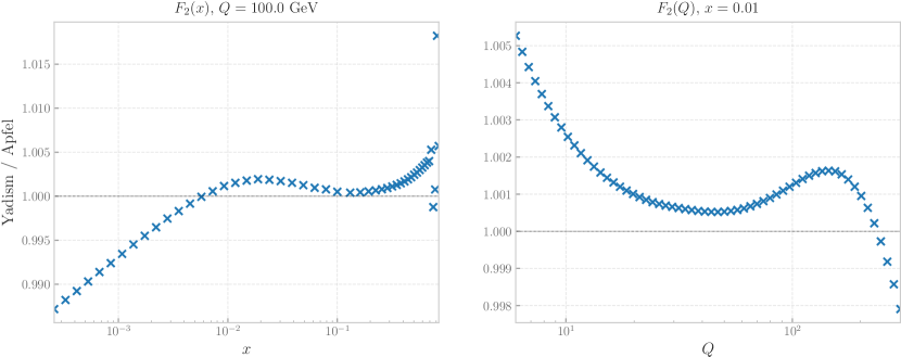
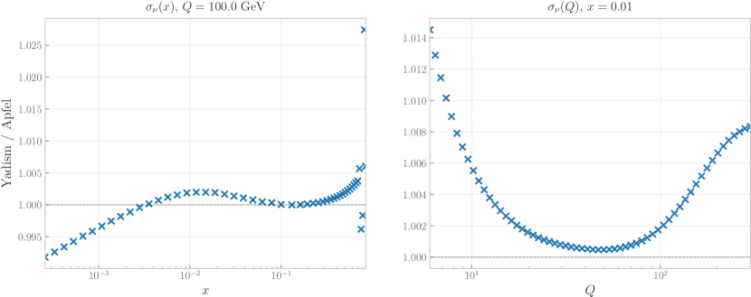
Figure B.1: The ratio between the YADISM and APFEL calculations of the neutrino-initiated structure function $F_{2}^{\nu A}(x,Q^{2})$ (top) and of the corresponding double-differential cross-sections (bottom panels) at NNLO for the same choice of input PDFs and theory settings. The benchmark comparison is presented both for fixed $Q=100$ GeV (left) and for fixed $x=0.01$ (right panels). A similar level of agreement is obtained for other DIS observables as well as for other regions of $(x,Q^{2})$ relevant for phenomenology.

Appendix C Nuclear effects in neutrino scattering

As compared to baseline predictions on a proton target, there are two effects that modify the neutrino scattering rates on nuclear targets. The first is related to the different content of up and down quarks, since for an isoscalar nuclear target the average nucleon has on 25% less (more) up (down) valence quarks than in a proton target, an effect which is more marked for non-isoscalar nuclei where $(A/2)>Z$. The second is associated to the modifications of the bound nucleon structure that take place in heavy nuclei when compared with their free-nucleon counterparts, and in the DIS region is quantified by the nuclear PDFs. In this appendix we illustrate the impact of these two effects on neutrino inelastic structure functions.

For a general nuclear target, the $F_{2}$ structure functions per nucleon at LO in terms of nPDFs are

$$F_{2}^{\nu A}(x,Q^{2}) = 2x\left(f^{(A)}_{\bar{u}}+f^{(A)}_{d}+f^{(A)}_{s}+f^{(A)}_{\bar{c}}\right)(x,Q^{2})\,,$$

$$F_{2}^{\bar{\nu}A}(x,Q^{2}) = 2x\left(f^{(A)}_{u}+f^{(A)}_{\bar{d}}+f^{(A)}_{\bar{s}}+f^{(A)}_{c}\right)(x,Q^{2})\,,$$ (C.1)

with similar expressions for $xF_{3}^{\nu A}$, and we assume that $Q^{2}$ is large enough so that QCD factorisation holds. For an isoscalar nucleus ($Z=A/2$) and neglecting nPDF effects, we can write

$$F_{2}^{\nu A}(x,Q^{2}) = 2x\left(\left(f^{(p)}_{\bar{u}}+f^{(p)}_{d}+f^{(p)}_{\bar{d}}+f^{(p)}_{u}\right)/2+f^{(p)}_{s}+f^{(p)}_{\bar{c}}\right)(x,Q^{2})\,,$$

$$F_{2}^{\bar{\nu}A}(x,Q^{2}) = 2x\left(\left(f^{(p)}_{u}+f^{(p)}_{\bar{d}}+f^{(p)}_{d}+f^{(p)}_{\bar{u}}\right)/2+f^{(p)}_{\bar{s}}+f^{(p)}_{c}\right)(x,Q^{2})\simeq F_{2}^{\nu A}(x,Q^{2})\,,$$ (C.2)

in terms of the free proton PDFs, and there the equality in the second equation holds neglecting the small charm and strange asymmetries. Comparing Eqns. (C.1) with (2.11), in the valence region $F_{2}^{\nu A}>F_{2}^{\nu p}$ and conversely for antineutrino scattering as a consequence of $f^{(p)}_{u}>f^{(p)}_{d}$. These differences cancel out when taking the sum of neutrino and antineutrino structure functions

$$F_{2}^{(\nu+\bar{\nu})A}(x,Q^{2})=2x\left(f^{(p)}_{\bar{u}}+f^{(p)}_{d}+f^{(p)}_{\bar{d}}+f^{(p)}_{u}+f^{(p)}_{s}+f^{(p)}_{\bar{c}}+f^{(p)}_{\bar{s}}+f^{(p)}_{c}\right)=F_{2}^{(\nu+\bar{\nu})p}(x,Q^{2})\,,$$ (C.3)

which coincides with the result for scattering on a free proton target.

Once isospin effects are corrected for, neutrino structure functions on nuclear targets can still differ from those associated to free nucleons due to genuine nuclear modifications. These are typically quantified by nuclear modification ratios of the form

$$R_{F_{i}}^{(A)}(x,Q^{2})={{AF_{i}^{\nu A}(x,Q^{2})}\over{\left(ZF_{i}^{\nu p}(x,Q^{2})+(A-Z)F_{i}^{\nu n}(x,Q^{2})\right)}}\,,$$ (C.4)

which are equal to unity if the bound-nucleon structure functions equal the free-nucleon ones. In the DIS region we can express these nuclear modification ratios in terms of the nPDFs

$$R_{f_{q}}^{(A)}(x,Q^{2})={{Af_{q}^{(N/A)}(x,Q^{2})}\over{\left(Zf_{q}^{(p)}(x,Q^{2})+(A-Z)f_{q}^{(n)}(x,Q^{2})\right)}}\,,$$ (C.5)

where $f^{(N/A)}$ indicates the PDFs of the average nucleon $N$ bound within a nuclei with $Z$ protons and $(A-Z)$ neutrons. Alternatively one can define

$$\widetilde{R}_{f_{q}}^{(A)}(x,Q^{2})={{f_{q}^{(N/A)}(x,Q^{2})}\over{f_{q}^{(p)}(x,Q^{2})}}\,,\qquad\widetilde{R}_{F_{i}}^{(A)}(x,Q^{2})={{F_{i}^{\nu A}(x,Q^{2})}\over{F_{i}^{\nu p}(x,Q^{2})}}\,,$$ (C.6)

which differ from unity due to both bound-nucleon modifications and due to the different valence quark content between the numerator and the denominator.

Fig. C.1 displays the nuclear structure function ratio Eq. (C.6) for $F_{2}$ and $xF_{3}$ at $Q=10$ GeV, where we show separately the ratios for the neutrino and antineutrino scattering as well as for their sum. Results are shown for two recent global nPDF determinations, nNNPDF3.0 (baseline in this work) and EPPS21 [112], which are in good agreement within uncertainties. In the case of nNNPDF3.0, we also display the nuclear modification ratio defined as in Eq. (C.4) where isospin effects are subtracted. The bands indicate the 90% CL intervals evaluated using the corresponding prescription for each nPDF set.

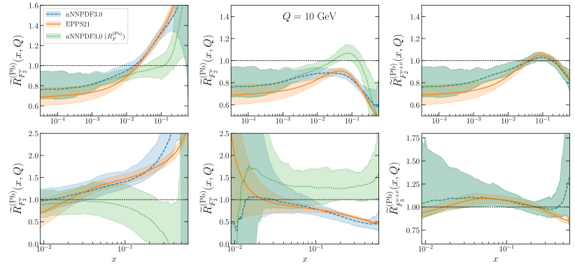
Figure C.1: The nuclear structure function ratio Eq. (C.6) for $F_{2}$ (upper) and $xF_{3}$ (lower panels) evaluated at LO on a lead target for nNNPDF3.0 and EPPS21 at $Q=10$ GeV. We display separately the ratios for the neutrino and antineutrino scattering, as well as for their sum. In the case of nNNPDF3.0, we also display the nuclear modification ratio defined as in Eq. (C.4) where isospin effects are subtracted. The bands indicate the 90% CL intervals.

As compared to a proton target, in the valence region ($x\mathrel{\hbox to0.0pt{\lower 4.0pt\hbox{\hskip 1.0pt$\sim$}\hss}\raise 1.0pt\hbox{$>$}}0.01$) one finds that the $F_{2}$ and $xF_{3}$ structure functions in lead are enhanced (suppressed) for neutrino (antineutrino scattering), mostly as a consequence of the increased content of down quarks in lead as compared to the proton. These differences cancel out in the sum of neutrino and antineutrino structure functions due to Eq. (C.3), and there the ratio Eq. (C.6) reduces to Eq. (C.4), namely the genuine nuclear modifications of bound nucleons and compared to free nucleons. Bound-nucleon modification ratios, Eq. (C.4), are small in the valence peak region, except at rather large-$x$ where structure functions are suppressed, and become more significant for $F_{2}$ in the sea quark region, $x\mathrel{\hbox to0.0pt{\lower 4.0pt\hbox{\hskip 1.0pt$\sim$}\hss}\raise 1.0pt\hbox{$<$}}0.01$, leading to a suppression of up to 25% as compared to the free-nucleon baseline. Therefore, from Fig. C.1 one concludes that in the valence region the dominant nuclear effects are the isospin-related ones, while in the sea region instead bound-nucleon modifications are important and need to be accounted for. These nuclear effects propagate to the inclusive cross section via Eq. (5.1), e.g. for neutrino scattering on lead one has an enhancement as compared to proton targets at low and intermediate energies and a suppression at high and ultra-high energies.

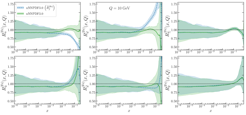
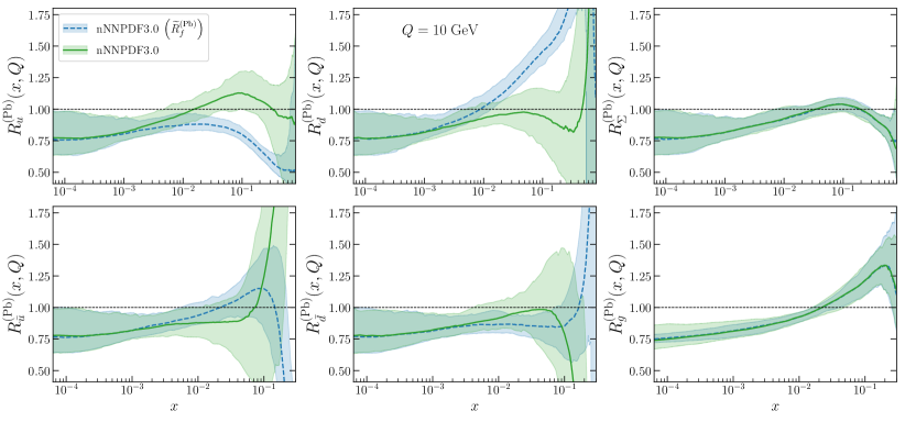
Figure C.2: The nuclear modification ratios in nNNPDF3.0 at $Q=10$ GeV for iron (upper) and lead (lower panels) targets. The bands indicate the 90% CL intervals. From left to right and from top to bottom we show the nuclear ratios corresponding to the up, down, singlet, antiup, antidown quark and the gluon nPDFs.

For completeness, we display in Fig. C.2 the corresponding nuclear modification ratios at the nPDF level in the case of the nNNPDF3.0 determination for both iron (Fe) and lead (Pb) targets. We compare the two definitions, Eqns. (C.5) and (C.6), differing in that isospin effects are accounted for in the former but not in the latter. As in Fig. C.1, the bands indicate the 90% CL intervals. In the valence region, one observes the expected suppression (enhancement) for up (down) quark nPDFs when using the ratio defined in Eq. (C.6). For isoscalar nPDF combinations such as the total quark singlet $\Sigma$ and the gluon the two nuclear ratio definitions coincide. From Fig. C.2 we observe the quark shadowing in the sea region also reported by the structure function ratios in the case of lead target, while for iron targets in this region the nuclear ratios are consistent with unity within uncertainties.

References

- [1] NuSTEC Collaboration, L. Alvarez-Ruso et al., “NuSTEC White Paper: Status and challenges of neutrino–nucleus scattering,” Prog. Part. Nucl. Phys. 100 (2018) 1–68, arXiv:1706.03621 [hep-ph].
- [2] A. B. Balantekin et al., “Snowmass Neutrino Frontier: Neutrino Interaction Cross Sections (NF06) Topical Group Report,” arXiv:2209.06872 [hep-ex].
- [3] KamLAND Collaboration, S. Abe et al., “Precision Measurement of Neutrino Oscillation Parameters with KamLAND,” Phys. Rev. Lett. 100 (2008) 221803, arXiv:0801.4589 [hep-ex].
- [4] DUNE Collaboration, R. Acciarri et al., “Long-Baseline Neutrino Facility (LBNF) and Deep Underground Neutrino Experiment (DUNE): Conceptual Design Report, Volume 2: The Physics Program for DUNE at LBNF,” arXiv:1512.06148 [physics.ins-det].
- [5] IceCube Collaboration, M. G. Aartsen et al., “Determining neutrino oscillation parameters from atmospheric muon neutrino disappearance with three years of IceCube DeepCore data,” Phys. Rev. D 91 no. 7, (2015) 072004, arXiv:1410.7227 [hep-ex].
- [6] IceCube-Gen2 Collaboration, M. G. Aartsen et al., “Combined sensitivity to the neutrino mass ordering with JUNO, the IceCube Upgrade, and PINGU,” Phys. Rev. D 101 no. 3, (2020) 032006, arXiv:1911.06745 [hep-ex].
- [7] KM3NeT Collaboration, S. Aiello et al., “Determining the neutrino mass ordering and oscillation parameters with KM3NeT/ORCA,” Eur. Phys. J. C 82 no. 1, (2022) 26, arXiv:2103.09885 [hep-ex].
- [8] J. L. Feng, I. Galon, F. Kling, and S. Trojanowski, “ForwArd Search ExpeRiment at the LHC,” Phys. Rev. D 97 no. 3, (2018) 035001, arXiv:1708.09389 [hep-ph].
- [9] FASER Collaboration, H. Abreu et al., “First Direct Observation of Collider Neutrinos with FASER at the LHC,” arXiv:2303.14185 [hep-ex].
- [10] SHiP Collaboration, C. Ahdida et al., “SND@LHC,” arXiv:2002.08722 [physics.ins-det].
- [11] L. A. Anchordoqui et al., “The Forward Physics Facility: Sites, experiments, and physics potential,” Phys. Rept. 968 (2022) 1–50, arXiv:2109.10905 [hep-ph].
- [12] J. L. Feng et al., “The Forward Physics Facility at the High-Luminosity LHC,” J. Phys. G 50 no. 3, (2023) 030501, arXiv:2203.05090 [hep-ex].
- [13] S. Alekhin et al., “A facility to Search for Hidden Particles at the CERN SPS: the SHiP physics case,” Rept. Prog. Phys. 79 no. 12, (2016) 124201, arXiv:1504.04855 [hep-ph].
- [14] M. Ackermann et al., “High-energy and ultra-high-energy neutrinos: A Snowmass white paper,” JHEAp 36 (2022) 55–110, arXiv:2203.08096 [hep-ph].
- [15] IceCube Collaboration, M. G. Aartsen et al., “Evidence for High-Energy Extraterrestrial Neutrinos at the IceCube Detector,” Science 342 (2013) 1242856, arXiv:1311.5238 [astro-ph.HE].
- [16] KM3Net Collaboration, S. Adrian-Martinez et al., “Letter of intent for KM3NeT 2.0” J. Phys. G 43 no. 8, (2016) 084001, arXiv:1601.07459 [astro-ph.IM].
- [17] GRAND Collaboration, J. Álvarez-Muñiz et al., “The Giant Radio Array for Neutrino Detection (GRAND): Science and Design,” Sci. China Phys. Mech. Astron. 63 no. 1, (2020) 219501, arXiv:1810.09994 [astro-ph.HE].
- [18] POEMMA Collaboration, A. V. Olinto et al., “The POEMMA (Probe of Extreme Multi-Messenger Astrophysics) observatory,” JCAP 06 (2021) 007, arXiv:2012.07945 [astro-ph.IM].
- [19] U. Mosel, “Neutrino event generators: foundation, status and future,” J. Phys. G 46 no. 11, (2019) 113001, arXiv:1904.11506 [hep-ex].
- [20] C. Andreopoulos et al., “The GENIE Neutrino Monte Carlo Generator,” Nucl. Instrum. Meth. A 614 (2010) 87–104, arXiv:0905.2517 [hep-ph].
- [21] C. Andreopoulos, C. Barry, S. Dytman, H. Gallagher, T. Golan, R. Hatcher, G. Perdue, and J. Yarba, “The GENIE Neutrino Monte Carlo Generator: Physics and User Manual,” arXiv:1510.05494 [hep-ph].
- [22] A. Garcia, R. Gauld, A. Heijboer, and J. Rojo, “Complete predictions for high-energy neutrino propagation in matter,” JCAP 09 (2020) 025, arXiv:2004.04756 [hep-ph].
- [23] O. Buss, T. Gaitanos, K. Gallmeister, H. van Hees, M. Kaskulov, O. Lalakulich, A. B. Larionov, T. Leitner, J. Weil, and U. Mosel, “Transport-theoretical Description of Nuclear Reactions,” Phys. Rept. 512 (2012) 1–124, arXiv:1106.1344 [hep-ph].
- [24] C. Juszczak, J. A. Nowak, and J. T. Sobczyk, “Simulations from a new neutrino event generator,” Nucl. Phys. B Proc. Suppl. 159 (2006) 211–216, arXiv:hep-ph/0512365.
- [25] M. L. Mangano et al., “Physics at the front end of a neutrino factory: A Quantitative appraisal,” arXiv:hep-ph/0105155.
- [26] J. M. Conrad, M. H. Shaevitz, and T. Bolton, “Precision measurements with high-energy neutrino beams,” Rev. Mod. Phys. 70 (1998) 1341–1392, arXiv:hep-ex/9707015.
- [27] J. Gao, L. Harland-Lang, and J. Rojo, “The Structure of the Proton in the LHC Precision Era,” Phys. Rept. 742 (2018) 1–121, arXiv:1709.04922 [hep-ph].
- [28] J. J. Ethier and E. R. Nocera, “Parton Distributions in Nucleons and Nuclei,” Ann. Rev. Nucl. Part. Sci. 70 (2020) 43–76, arXiv:2001.07722 [hep-ph].
- [29] K. Kovařík, P. M. Nadolsky, and D. E. Soper, “Hadronic structure in high-energy collisions,” Rev. Mod. Phys. 92 no. 4, (2020) 045003, arXiv:1905.06957 [hep-ph].
- [30] S. Moch, M. Rogal, and A. Vogt, “Differences between charged-current coefficient functions,” Nucl. Phys. B 790 (2008) 317–335, arXiv:0708.3731 [hep-ph].
- [31] S. Moch, J. A. M. Vermaseren, and A. Vogt, “Third-order QCD corrections to the charged-current structure function F(3),” Nucl. Phys. B 813 (2009) 220–258, arXiv:0812.4168 [hep-ph].
- [32] S. Moch, B. Ruijl, T. Ueda, J. A. M. Vermaseren, and A. Vogt, “Low moments of the four-loop splitting functions in QCD,” Phys. Lett. B 825 (2022) 136853, arXiv:2111.15561 [hep-ph].
- [33] J. McGowan, T. Cridge, L. A. Harland-Lang, and R. S. Thorne, “Approximate N3LO Parton Distribution Functions with Theoretical Uncertainties: MSHT20aN3LO PDFs,” arXiv:2207.04739 [hep-ph].
- [34] S. Forte, E. Laenen, P. Nason, and J. Rojo, “Heavy quarks in deep-inelastic scattering,” Nucl. Phys. B 834 (2010) 116–162, arXiv:1001.2312 [hep-ph].
- [35] M. Guzzi, P. M. Nadolsky, H.-L. Lai, and C. P. Yuan, “General-Mass Treatment for Deep Inelastic Scattering at Two-Loop Accuracy,” Phys. Rev. D 86 (2012) 053005, arXiv:1108.5112 [hep-ph].
- [36] R. S. Thorne and R. G. Roberts, “An Ordered analysis of heavy flavor production in deep inelastic scattering,” Phys. Rev. D 57 (1998) 6871–6898, arXiv:hep-ph/9709442.
- [37] R. D. Ball, V. Bertone, M. Bonvini, S. Forte, P. Groth Merrild, J. Rojo, and L. Rottoli, “Intrinsic charm in a matched general-mass scheme,” Phys. Lett. B 754 (2016) 49–58, arXiv:1510.00009 [hep-ph].
- [38] M. Bonvini, S. Marzani, J. Rojo, L. Rottoli, M. Ubiali, R. D. Ball, V. Bertone, S. Carrazza, and N. P. Hartland, “Parton distributions with threshold resummation,” JHEP 09 (2015) 191, arXiv:1507.01006 [hep-ph].
- [39] M. Bonvini, S. Marzani, and T. Peraro, “Small- resummation from HELL,” Eur. Phys. J. C 76 no. 11, (2016) 597, arXiv:1607.02153 [hep-ph].
- [40] R. D. Ball, V. Bertone, M. Bonvini, S. Marzani, J. Rojo, and L. Rottoli, “Parton distributions with small-x resummation: evidence for BFKL dynamics in HERA data,” Eur. Phys. J. C 78 no. 4, (2018) 321, arXiv:1710.05935 [hep-ph].
- [41] V. Bertone, R. Gauld, and J. Rojo, “Neutrino Telescopes as QCD Microscopes,” JHEP 01 (2019) 217, arXiv:1808.02034 [hep-ph].
- [42] M. H. Reno, “Electromagnetic structure functions and neutrino nucleon scattering,” Phys. Rev. D 74 (2006) 033001, arXiv:hep-ph/0605295.
- [43] U.-K. Yang and A. Bodek, “Parton distributions, , and higher twist effects at high x,” Phys. Rev. Lett. 82 (1999) 2467–2470, arXiv:hep-ph/9809480.
- [44] A. Bodek and U. K. Yang, “Modeling deep inelastic cross-sections in the few GeV region,” Nucl. Phys. B Proc. Suppl. 112 (2002) 70–76, arXiv:hep-ex/0203009.
- [45] A. Bodek and U. K. Yang, “Modeling neutrino and electron scattering inelastic cross- sections in the few GeV region with effective LO PDFs TV Leading Order,” in 2nd International Workshop on Neutrino-Nucleus Interactions in the Few GeV Region. 8, 2003. arXiv:hep-ex/0308007.
- [46] A. Bodek, I. Park, and U.-k. Yang, “Improved low Q**2 model for neutrino and electron nucleon cross sections in few GeV region,” Nucl. Phys. B Proc. Suppl. 139 (2005) 113–118, arXiv:hep-ph/0411202.
- [47] A. Bodek and U.-k. Yang, “Axial and Vector Structure Functions for Electron- and Neutrino- Nucleon Scattering Cross Sections at all using Effective Leading order Parton Distribution Functions,” arXiv:1011.6592 [hep-ph].
- [48] A. Bodek, U. K. Yang, and Y. Xu, “Inelastic Axial and Vector Structure Functions for Lepton-Nucleon Scattering 2021 Update,” arXiv:2108.09240 [hep-ph].
- [49] M. Glück, E. Reya, and A. Vogt, “Dynamical parton distributions revisited,” Eur. Phys. J. C 5 (1998) 461–470, arXiv:hep-ph/9806404.
- [50] A. Connolly, R. S. Thorne, and D. Waters, “Calculation of High Energy Neutrino-Nucleon Cross Sections and Uncertainties Using the MSTW Parton Distribution Functions and Implications for Future Experiments,” Phys. Rev. D 83 (2011) 113009, arXiv:1102.0691 [hep-ph].
- [51] A. Cooper-Sarkar and S. Sarkar, “Predictions for high energy neutrino cross-sections from the ZEUS global PDF fits,” JHEP 01 (2008) 075, arXiv:0710.5303 [hep-ph].
- [52] A. Cooper-Sarkar, P. Mertsch, and S. Sarkar, “The high energy neutrino cross-section in the Standard Model and its uncertainty,” JHEP 08 (2011) 042, arXiv:1106.3723 [hep-ph].
- [53] K. Xie, J. Gao, T. J. Hobbs, D. R. Stump, and C. P. Yuan, “High-energy neutrino deeply inelastic scattering cross sections from 100 GeV to 1000 EeV,” arXiv:2303.13607 [hep-ph].
- [54] NNPDF Collaboration, L. Del Debbio, S. Forte, J. I. Latorre, A. Piccione, and J. Rojo, “Neural network determination of parton distributions: The Nonsinglet case,” JHEP 03 (2007) 039, arXiv:hep-ph/0701127.
- [55] NNPDF Collaboration, R. D. Ball et al., “Parton distributions from high-precision collider data,” Eur. Phys. J. C 77 no. 10, (2017) 663, arXiv:1706.00428 [hep-ph].
- [56] NNPDF Collaboration, R. D. Ball, L. Del Debbio, S. Forte, A. Guffanti, J. I. Latorre, A. Piccione, J. Rojo, and M. Ubiali, “A Determination of parton distributions with faithful uncertainty estimation,” Nucl. Phys. B 809 (2009) 1–63, arXiv:0808.1231 [hep-ph]. [Erratum: Nucl.Phys.B 816, 293 (2009)].
- [57] R. D. Ball, L. Del Debbio, S. Forte, A. Guffanti, J. I. Latorre, J. Rojo, and M. Ubiali, “A first unbiased global NLO determination of parton distributions and their uncertainties,” Nucl. Phys. B 838 (2010) 136–206, arXiv:1002.4407 [hep-ph].
- [58] R. D. Ball et al., “Parton Distribution Benchmarking with LHC Data,” JHEP 04 (2013) 125, arXiv:1211.5142 [hep-ph].
- [59] NNPDF Collaboration, R. D. Ball et al., “Parton distributions for the LHC Run II,” JHEP 04 (2015) 040, arXiv:1410.8849 [hep-ph].
- [60] NNPDF Collaboration, R. D. Ball et al., “The path to proton structure at 1% accuracy,” Eur. Phys. J. C 82 no. 5, (2022) 428, arXiv:2109.02653 [hep-ph].
- [61] NNPDF Collaboration, R. D. Ball et al., “An open-source machine learning framework for global analyses of parton distributions,” Eur. Phys. J. C 81 no. 10, (2021) 958, arXiv:2109.02671 [hep-ph].
- [62] NNPDF Collaboration, L. Del Debbio, S. Forte, J. I. Latorre, A. Piccione, and J. Rojo, “Unbiased determination of the proton structure function F(2)**p with faithful uncertainty estimation,” JHEP 03 (2005) 080, arXiv:hep-ph/0501067.
- [63] S. Forte, L. Garrido, J. I. Latorre, and A. Piccione, “Neural network parametrization of deep inelastic structure functions,” JHEP 05 (2002) 062, arXiv:hep-ph/0204232.
- [64] A. Candido, F. Hekhorn, and G. Magni, “EKO: Evolution Kernel Operators,” arXiv:2202.02338 [hep-ph].
- [65] R. Abdul Khalek, R. Gauld, T. Giani, E. R. Nocera, T. R. Rabemananjara, and J. Rojo, “nNNPDF3.0: evidence for a modified partonic structure in heavy nuclei,” Eur. Phys. J. C 82 no. 6, (2022) 507, arXiv:2201.12363 [hep-ph].
- [66] A. Buckley, J. Ferrando, S. Lloyd, K. Nordström, B. Page, M. Rüfenacht, M. Schönherr, and G. Watt, “LHAPDF6: parton density access in the LHC precision era,” Eur. Phys. J. C 75 (2015) 132, arXiv:1412.7420 [hep-ph].
- [67] J. Gao, “Massive charged-current coefficient functions in deep-inelastic scattering at NNLO and impact on strange-quark distributions,” JHEP 02 (2018) 026, arXiv:1710.04258 [hep-ph].
- [68] D. J. Gross and C. H. Llewellyn Smith, “High-energy neutrino - nucleon scattering, current algebra and partons,” Nucl. Phys. B 14 (1969) 337–347.
- [69] V. Bertone, S. Carrazza, and J. Rojo, “APFEL: A PDF Evolution Library with QED corrections,” Comput. Phys. Commun. 185 (2014) 1647–1668, arXiv:1310.1394 [hep-ph].
- [70] R. D. Ball, V. Bertone, F. Cerutti, L. Del Debbio, S. Forte, A. Guffanti, J. I. Latorre, J. Rojo, and M. Ubiali, “Impact of Heavy Quark Masses on Parton Distributions and LHC Phenomenology,” Nucl. Phys. B 849 (2011) 296–363, arXiv:1101.1300 [hep-ph].
- [71] R. Gauld and J. Rojo, “Precision determination of the small- gluon from charm production at LHCb,” Phys. Rev. Lett. 118 no. 7, (2017) 072001, arXiv:1610.09373 [hep-ph].
- [72] R. Abdul Khalek, J. J. Ethier, J. Rojo, and G. van Weelden, “nNNPDF2.0: quark flavor separation in nuclei from LHC data,” JHEP 09 (2020) 183, arXiv:2006.14629 [hep-ph].
- [73] R. D. Ball, E. R. Nocera, and J. Rojo, “The asymptotic behaviour of parton distributions at small and large ,” Eur. Phys. J. C 76 no. 7, (2016) 383, arXiv:1604.00024 [hep-ph].
- [74] ArgoNeuT Collaboration, C. Anderson et al., “First Measurements of Inclusive Muon Neutrino Charged Current Differential Cross Sections on Argon,” Phys. Rev. Lett. 108 (2012) 161802, arXiv:1111.0103 [hep-ex].
- [75] MicroBooNE Collaboration, P. Abratenko et al., “First Measurement of Inclusive Muon Neutrino Charged Current Differential Cross Sections on Argon at 0.8 GeV with the MicroBooNE Detector,” Phys. Rev. Lett. 123 no. 13, (2019) 131801, arXiv:1905.09694 [hep-ex].
- [76] T2K Collaboration, K. Abe et al., “First measurement of the charged-current cross section on a water target without pions in the final state,” Phys. Rev. D 97 no. 1, (2018) 012001, arXiv:1708.06771 [hep-ex].
- [77] MINERvA Collaboration, J. Mousseau et al., “Measurement of Partonic Nuclear Effects in Deep-Inelastic Neutrino Scattering using MINERvA,” Phys. Rev. D 93 no. 7, (2016) 071101, arXiv:1601.06313 [hep-ex].
- [78] BEBC WA59 Collaboration, K. Varvell et al., “Measurement of the Structure Functions F2 and Xf3 and Comparison With QCD Predictions Including Kinematical and Dynamical Higher Twist Effects,” Z. Phys. C 36 (1987) 1.
- [79] E. Oltman et al., “Nucleon structure functions from high energy neutrino interactions,” Z. Phys. C 53 (1992) 51–71.
- [80] CHARM Collaboration, F. Bergsma et al., “Experimental Study of the Nucleon Structure Functions and of the Gluon Distribution from Charged Current Neutrino and anti-neutrinos Interactions,” Phys. Lett. B 123 (1983) 269.
- [81] CHORUS Collaboration, G. Onengut et al., “Measurement of nucleon structure functions in neutrino scattering,” Phys. Lett. B 632 (2006) 65–75.
- [82] J. P. Berge et al., “A Measurement of Differential Cross-Sections and Nucleon Structure Functions in Charged Current Neutrino Interactions on Iron,” Z. Phys. C49 (1991) 187–224.
- [83] NuTeV Collaboration, M. Tzanov et al., “Precise measurement of neutrino and anti-neutrino differential cross sections,” Phys. Rev. D 74 (2006) 012008, arXiv:hep-ex/0509010.
- [84] R. D. Ball et al., “Parton distributions with LHC data,” Nucl. Phys. B 867 (2013) 244–289, arXiv:1207.1303 [hep-ph].
- [85] NNPDF Collaboration, E. R. Nocera, R. D. Ball, S. Forte, G. Ridolfi, and J. Rojo, “A first unbiased global determination of polarized PDFs and their uncertainties,” Nucl. Phys. B 887 (2014) 276–308, arXiv:1406.5539 [hep-ph].
- [86] NNPDF Collaboration, R. D. Ball, S. Forte, A. Guffanti, E. R. Nocera, G. Ridolfi, and J. Rojo, “Unbiased determination of polarized parton distributions and their uncertainties,” Nucl. Phys. B 874 (2013) 36–84, arXiv:1303.7236 [hep-ph].
- [87] NNPDF Collaboration, R. Abdul Khalek, J. J. Ethier, and J. Rojo, “Nuclear parton distributions from lepton-nucleus scattering and the impact of an electron-ion collider,” Eur. Phys. J. C 79 no. 6, (2019) 471, arXiv:1904.00018 [hep-ph].
- [88] NNPDF Collaboration, V. Bertone, N. P. Hartland, E. R. Nocera, J. Rojo, and L. Rottoli, “Charged hadron fragmentation functions from collider data,” Eur. Phys. J. C 78 no. 8, (2018) 651, arXiv:1807.03310 [hep-ph].
- [89] NNPDF Collaboration, V. Bertone, S. Carrazza, N. P. Hartland, E. R. Nocera, and J. Rojo, “A determination of the fragmentation functions of pions, kaons, and protons with faithful uncertainties,” Eur. Phys. J. C 77 no. 8, (2017) 516, arXiv:1706.07049 [hep-ph].
- [90] M. Abadi, A. Agarwal, P. Barham, E. Brevdo, Z. Chen, C. Citro, G. S. Corrado, A. Davis, J. Dean, M. Devin, S. Ghemawat, I. Goodfellow, A. Harp, G. Irving, M. Isard, Y. Jia, R. Jozefowicz, L. Kaiser, M. Kudlur, J. Levenberg, D. Mané, R. Monga, S. Moore, D. Murray, C. Olah, M. Schuster, J. Shlens, B. Steiner, I. Sutskever, K. Talwar, P. Tucker, V. Vanhoucke, V. Vasudevan, F. Viégas, O. Vinyals, P. Warden, M. Wattenberg, M. Wicke, Y. Yu, and X. Zheng, “TensorFlow: Large-scale machine learning on heterogeneous systems,” 2015. https://www.tensorflow.org/. Software available from tensorflow.org.
- [91] D. P. Kingma and J. Ba, “Adam: A method for stochastic optimization,” in 3rd International Conference on Learning Representations, ICLR 2015, San Diego, CA, USA, May 7-9, 2015, Conference Track Proceedings, Y. Bengio and Y. LeCun, eds. 2015. http://arxiv.org/abs/1412.6980.
- [92] NNPDF Collaboration, R. D. Ball, L. Del Debbio, S. Forte, A. Guffanti, J. I. Latorre, J. Rojo, and M. Ubiali, “Fitting Parton Distribution Data with Multiplicative Normalization Uncertainties,” JHEP 05 (2010) 075, arXiv:0912.2276 [hep-ph].
- [93] NNPDF Collaboration, R. Abdul Khalek et al., “Parton Distributions with Theory Uncertainties: General Formalism and First Phenomenological Studies,” Eur. Phys. J. C 79 no. 11, (2019) 931, arXiv:1906.10698 [hep-ph].
- [94] NNPDF Collaboration, R. Abdul Khalek et al., “A first determination of parton distributions with theoretical uncertainties,” Eur. Phys. J. C (2019) 79:838, arXiv:1905.04311 [hep-ph].
- [95] K. F. Muzakka et al., “Compatibility of neutrino DIS data and its impact on nuclear parton distribution functions,” Phys. Rev. D 106 no. 7, (2022) 074004, arXiv:2204.13157 [hep-ph].
- [96] K. Kovarik, I. Schienbein, F. I. Olness, J. Y. Yu, C. Keppel, J. G. Morfin, J. F. Owens, and T. Stavreva, “Nuclear Corrections in Neutrino-Nucleus DIS and Their Compatibility with Global NPDF Analyses,” Phys. Rev. Lett. 106 (2011) 122301, arXiv:1012.0286 [hep-ph].
- [97] H. Paukkunen and C. A. Salgado, “Compatibility of neutrino DIS data and global analyses of parton distribution functions,” JHEP 07 (2010) 032, arXiv:1004.3140 [hep-ph].
- [98] IceCube Collaboration, M. G. Aartsen et al., “Measurements using the inelasticity distribution of multi-TeV neutrino interactions in IceCube,” Phys. Rev. D 99 no. 3, (2019) 032004, arXiv:1808.07629 [hep-ex].
- [99] F. Kling and L. J. Nevay, “Forward neutrino fluxes at the LHC,” Phys. Rev. D 104 no. 11, (2021) 113008, arXiv:2105.08270 [hep-ph].
- [100] W. Bai, M. Diwan, M. V. Garzelli, Y. S. Jeong, and M. H. Reno, “Far-forward neutrinos at the Large Hadron Collider,” JHEP 06 (2020) 032, arXiv:2002.03012 [hep-ph].
- [101] M. Constantinou et al., “Parton distributions and lattice-QCD calculations: Toward 3D structure,” Prog. Part. Nucl. Phys. 121 (2021) 103908, arXiv:2006.08636 [hep-ph].
- [102] M. Botje, “QCDNUM: Fast QCD Evolution and Convolution,” Comput. Phys. Commun. 182 (2011) 490–532, arXiv:1005.1481 [hep-ph].
- [103] S. Carrazza, E. R. Nocera, C. Schwan, and M. Zaro, “PineAPPL: combining EW and QCD corrections for fast evaluation of LHC processes,” JHEP 12 (2020) 108, arXiv:2008.12789 [hep-ph].
- [104] A. Candido and F. Hekhorn, “YADISM: Yet Another DIS Module,”. in preparation.
- [105] T. Carli, D. Clements, A. Cooper-Sarkar, C. Gwenlan, G. P. Salam, F. Siegert, P. Starovoitov, and M. Sutton, “A posteriori inclusion of parton density functions in NLO QCD final-state calculations at hadron colliders: The APPLGRID Project,” Eur. Phys. J. C 66 (2010) 503–524, arXiv:0911.2985 [hep-ph].
- [106] fastNLO Collaboration, M. Wobisch, D. Britzger, T. Kluge, K. Rabbertz, and F. Stober, “Theory-Data Comparisons for Jet Measurements in Hadron-Induced Processes,” arXiv:1109.1310 [hep-ph].
- [107] V. Bertone, R. Frederix, S. Frixione, J. Rojo, and M. Sutton, “aMCfast: automation of fast NLO computations for PDF fits,” JHEP 08 (2014) 166, arXiv:1406.7693 [hep-ph].
- [108] N. Laurenti, “Construction of a next to next to next to leading order approximation for heavy flavour production in deep inelastic scattering with quark masses,”. MSc thesis, Universita Roma I, 2021.
- [109] H. Kawamura, N. A. Lo Presti, S. Moch, and A. Vogt, “On the next-to-next-to-leading order QCD corrections to heavy-quark production in deep-inelastic scattering,” Nucl. Phys. B 864 (2012) 399–468, arXiv:1205.5727 [hep-ph].
- [110] W. L. van Neerven and A. Vogt, “NNLO evolution of deep inelastic structure functions: The Singlet case,” Nucl. Phys. B 588 (2000) 345–373, arXiv:hep-ph/0006154.
- [111] W. L. van Neerven and A. Vogt, “Nonsinglet structure functions beyond the next-to-next-to-leading order,” Nucl. Phys. B 603 (2001) 42–68, arXiv:hep-ph/0103123.
- [112] K. J. Eskola, P. Paakkinen, H. Paukkunen, and C. A. Salgado, “EPPS21: a global QCD analysis of nuclear PDFs,” Eur. Phys. J. C 82 no. 5, (2022) 413, arXiv:2112.12462 [hep-ph].