Virgo Detector Characterization and Data Quality during the O3 run

Abstract

The Advanced Virgo detector has contributed with its data to the rapid growth of the number of detected gravitational-wave signals in the past few years, alongside the two LIGO instruments. First, during the last month of the Observation Run 2 (O2) in August 2017 (with, most notably, the compact binary mergers GW170814 and GW170817) and then during the full Observation Run 3 (O3): an 11 months data taking period, between April 2019 and March 2020, that led to the addition of about 80 events to the catalog of transient gravitational-wave sources maintained by LIGO, Virgo and KAGRA. These discoveries and the manifold exploitation of the detected waveforms require an accurate characterization of the quality of the data, such as continuous study and monitoring of the detector noise. These activities, collectively named detector characterization or DetChar, span the whole workflow of the Virgo data, from the instrument front-end to the final analysis. They are described in details in the following article, with a focus on the associated tools, the results achieved by the Virgo DetChar group during the O3 run and the main prospects for future data-taking periods with an improved detector.

1 Introduction

A century after being predicted by Albert Einstein in the framework of general relativity, gw have been detected by a global network of ground-based interferometric detectors [1]. The LIGO [2] and Virgo [3] collaborations, now joined by the KAGRA [4] collaboration, have observed in the past six years dozens of gw signals coming from merging compact binary systems. Compact binaries composed of two bh, two ns, or both kinds of compact object have all been observed so far. GW150914 [1], the first gw signal ever detected (at that time by the two Advanced LIGO detectors) was a binary bh merger. Two years later, shortly after the adv detector had started operating, the 3-interferometer network detected the signal GW170817 [5], emitted by the fusion of two ns and associated with counterparts in the entire electromagnetic spectrum, leading to the birth of multi-messenger astronomy with gw. More recently, LIGO, Virgo and KAGRA (“LVK”) have announced the first detections of ns-bh mergers in data taken in January 2020 [6].

All events add up in a gw Transient Catalog whose first four versions— GWTC-1 [7], GWTC-2 [8], GWTC-2.1 [9] and GWTC-3 [10]— have been released. Such a catalog allows scientists to go beyond the detections themselves and probe the populations of compact stars, estimate the merger rate of binary systems, test general relativity in the strong-field regime, and perform searches for counterparts using archival data from other observatories. The reconstructed gw strain data—the so-called $h(t)$ streams—are regularly released in chunks of several months on the gwosc website [11].

Producing these results requires a thorough characterization of the data quality, a large part of which involves studying and monitoring the noise of gw detectors. This activity, often referred to as detector characterization or DetChar, is an expertise which has been constructed over many years, starting with the initial detectors [12, 13]. Analysis methods and tools have been developed and implemented to characterize the Virgo data both with low latency and offline. They cover a physics-driven chain that starts from the raw data recorded by the instrument and extends all the way to the final set of gw events and the related analysis. The results of DetChar analyses are used to improve the detector performance during commissioning periods and to maximize the sensitivity to gw signals during an Observing Run, when science-quality data is recorded.

This paper reports the work of the Virgo DetChar group over the past few years, with an emphasis on the preparation for the third LIGO-Virgo observing run, O3 (April 2019— March 2020), on the activities during O3, as well as on the final results achieved after the run and the experience accumulated in view of the future runs of the LVK network. These achievements stem from the developments made before and during the O2 run (for Virgo: 25 days of data taking in August 2017) and those will also be described here when appropriate.

Section 2 provides an overview of the adv detector configuration during the O3 run, preceded by a short summary of the path that led to this data taking period. The same section also introduces notions and concepts that will be extensively used in the rest of the article, and defines a few related abbreviations. Then, Section 3 summarizes the O3 run from a Virgo perspective: how the data taking was organized, what the performance of the detector and the final O3 dataset were. Section 4 describes the main DetChar tools, classified by categories: monitoring tools; generic multi-purpose tools; tools to study noise transients; tools to investigate the noise spectrum; and finally, common LIGO-Virgo tools. The description of each tool has been kept short in the main text; additional information regarding those that are not referenced in the literature is provided in A. Section 5 presents the Virgo online data quality framework built for the O3 run. Section 6 deals with the framework developed to vet signals candidate to be released as public alerts to the astronomical community. Section 7 presents the main DetChar analyses done on the O3 dataset to study noise transients; their impact on gw searches; the noise spectrum; and the final validation of events. Finally, Section 8 provides some information about the ongoing preparation of the future O4 run, that is scheduled to start at the end of 2022.

A list of the main abbreviations used throughout the article is provided as well, for reference.

2 The Advanced Virgo Detector

This section focuses on the Virgo detector during the O3 run. First, we briefly review the main steps of the adv project up to the beginning of O3. In particular, we emphasize its participation to the last four weeks of the O2 run in August 2017 that were rich of discoveries. Then, we summarize the activities during the 1.5 year-long shutdown between O2 and O3 that allowed the Virgo Collaboration to improve the instrument significantly. Finally, we describe the detector configuration during O3 and present the main features of the data it has collected.

2.1 The path to the O3 run

Virgo [14] is an interferometric detector of gw located at the European Gravitational Observatory (EGO) in Cascina, Italy. The adv project [3] allowed to upgrade the original instrument to a second-generation detector, similarly to what LIGO has done with its two interferometers [2], located in Hanford (WA, USA) and Livingston (LA, USA). The funding of adv was approved in December 2009 by CNRS (France) and INFN (Italy), with an in-kind contribution from Nikhef (The Netherlands). The decommissioning of the first-generation Virgo detector started in Fall 2011, after the completion of the science run VSR4 [15], pursued together with the GEO600 detector [16] (the Advanced LIGO upgrade project had already started). The installation of the Avanced Virgo equipment started mid-2012 and was completed in 2016. The upgraded interferometer was robustly controlled in March 2017 and the next few months were dedicated to commissioning activities: noise hunting and sensitivity improvement. At the end of July, the detector was very stable and had a sensitivity corresponding to a bns range of ${\sim}30$ Mpc, that is more than a factor two above the performance of the Virgo+ detector during the VSR4 run.

Therefore, adv started taking data on August 1 2017, joining the second Observing Run, O2, which had started on November 30, 2016 for the two LIGO interferometers [17]. On August 14, 2017, the adv detector made its first detection of a gw. That event, labelled GW170814, was also recorded by the two LIGO interferometers. It was the first ever triple detection of a binary black hole coalescence, allowing an unprecedented accuracy in the localization of the source in the sky [18]. A few days later, on August 17, the three interferometers jointly detected, for the first time, a gw emitted by the coalescence of two neutron stars [19]. This event, known as GW170817, was accompanied by the almost simultaneous detection of a gamma-ray burst by the Fermi Gamma-ray and Integral space telescopes [20]. The accuracy in the localization of the gw source (approx. 30$\deg^{2}$) allowed to identify the optical counterpart in the galaxy NGC4993 [21]. The O2 run ended on August 25, 2017.

The LIGO-Virgo shutdown between O2 and the third Observing Run, O3, lasted 19 months. On the Virgo side, it was divided into four periods.

• A post-O2 commissioning phase, until early December 2017.
  The goal was twofold: to make a series of measurements on the O2 detector configuration that would have been too invasive during the run and to perform some tests to try to further improve the instrument.

• Hardware upgrades until mid-March 2018. Four main projects were pursued:

  • The re-installation of the monolithic suspensions and various vacuum upgrades.
    The steel wires, with which the adv arm cavity mirrors had been suspended for the O2 run, were replaced with quartz fibers. Monolithic suspensions, successfully tested in the Virgo+ configuration [22, 23], had been foreseen in the adv Technical Design Report [24]. Yet, multiple breakings of fused silica fibers when installed in vacuum were observed in Fall 2016, forcing the recourse of steel wires to preserve the participation of Virgo to the O2 run. The fiber breaking issue was eventually demonstrated to be caused by a spurious dust contamination generated by some vacuum pumps [25]. Therefore, the Virgo vacuum system was improved in order to avoid contamination with dust particles while the suspension fibers were shielded.

  • A higher laser power.
    The laser power injected into the interferometer was increased, in order to reduce the photon shot noise, limiting the high-frequency sensitivity: 10 W (19 W) were injected in Virgo during the O2 run (at the beginning of the O3 run).

  • The installation of a squeezed light source.
    This allows to further reduce the shot noise limit at high frequencies by modifying the quantum properties of the light coming out of the interferometer [26].

  • The test installation of an array of seismic sensors.
    An in-depth characterization of the seismic noise field at the test mass locations was performed in order to prepare for the subtraction of the Newtonian noise contribution that may limit the low-frequency sensitivity in the future [27].

• A commissioning period, until Fall 2018, to improve the sensitivity and the duty cycle of the detector.

• Finally, the transition phase to the O3 run, that officially started on April 1st, 2019 at 15:00 UTC.

2.2 The O3 configuration

The adv detector has been designed to achieve a sensitivity about one order of magnitude better than that of the initial Virgo, corresponding to an increase in the detection rate by about three orders of magnitude. The adv design choices were made on the basis of the outcome of the different research and development activities carried out within the gw community and the experience gained with Virgo, while also taking into account budget and schedule constraints.

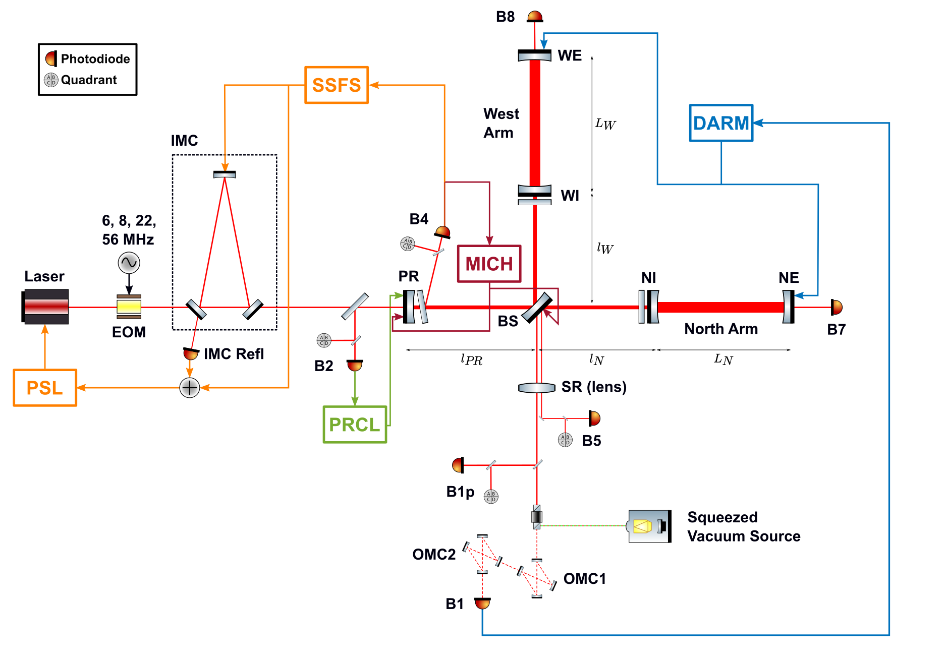
Figure 1: Schematics of the adv configuration during the O3 run (not to scale), showing optics, photodiodes and quadrant photodiodes, such as the main components of the global feedback system used to steer the detector. The suspended optical benches introduced in the text are not represented here. This figure is taken from [28].

The simplified optical schematic of adv during the O2 and O3 runs is shown in Figure 1. In the following, we briefly outline the different parts of the detector layout and define the main abbreviations that are labelled on the schematic or used later in the article. Further information about the O3 configuration and control system of the Virgo detector can be found in [28].

The Virgo power-stabilized infrared laser beam (PSL, wavelength: 1.064 $\mu$m) is filtered at the interferometer input by a 144 m triangular cavity called the imc; the two flat mirrors of the imc are located on the first suspended injection bench (SIB1), that also hosts various optics for beam matching. Then, the beam goes through the partially reflective pr mirror before being split into two perpendicular beams at the bs mirror. The two 3 km-long arms hosting Fabry-Perot cavities are called "North" and "West" as they are roughly oriented along these geographical directions. The cavity mirrors closest (furthest away) from the bs are called "input" ("end") mirrors. So, following these conventions, the test masses (the four mirrors forming the two 3-km long Fabry-Perot cavities) are labelled ni, ne, wi and we. Both arms end with a suspended terminal bench—called sneb or sweb—hosting a photodiode (B7 or B8) receiving the cavity transmitted beam. After propagation and storage in the kilometric cavities, the arm beams recombine on the bs and the beam resulting from this interference goes to the interferometer output port. As indicated in Figure 1, the location of the foreseen sr mirror was occupied by the first lens of the detection system during the O3 run (and during O2 as well). The installation of that additional mirror only took place during the shutdown period that followed the end of O3. Further downstream is the place where the beam from the frequency-indepedent squeezed light source enters the detector. Finally, prior to being detected on the dark fringe port B1 photodiode located on the suspended detection bench 2 (SDB2), the output port beam is filtered in sequence by two omc cavities, omc1 and omc2, located on the suspended detection bench 1 (SDB1).

A complex active feedback system, made of several automated control feedback loops, is necessary to bring the detector to its global working point and maintain it there. In particular, it aims at controlling the four main longitudinal dof of the adv detector in its O2-O3 configuration that are defined below. This global control relies on radio-frequency sidebands for the carrier beam that are generated by the eom located in between the laser source and the IMC on Figure 1. The 6, 8 and 56 Mhz sidebands are used to control the interferometer, while the 22 MHz one is used to control the injection system.

• The mich, $l_{N}-l_{W}$, sets the destructive interference (‘dark fringe’) optimal condition.

• Theprcl, $l_{PR}+(l_{N}+l_{W})/2$, that must be resonant.

• The lengths of the kilometric Fabry-Perot cavities, $L_{N}$ and $L_{W}$, that must be resonant as well, or rather their sum and difference that are more physical.

  • The carm, $(L_{N}+L_{W})/2$, used as a length etalon by the ssfs to stabilize further the frequency of the input laser.

  • The darm, $L_{N}-L_{W}$, the quantity sensitive to a passing gw.

2.3 Virgo data and DetChar products

The GW strain data stream reconstructed at the Virgo detector is dominated by noise with, up-to-now, rare and weak gw signals. That noise results from several contributions that can be roughly classified into two main categories.

• Fundamental noises, that are inherent to the instrument and represent the ultimate limit of its sensitivity. Their combination is usually Gaussian and stationary, meaning that their properties do not change in time.

• Various varying noise artifacts, whose origins are manifold (hardware components of the detector, feedback control loops, interaction with the external environment, etc.) and that represent potential issues, not only because they may impact the running of the instrument but also—and above all—because they show up in the background of searches for gw, limiting thus their sensitivity. Noise transients, called glitches, can either look like real signals or overlap in time with one, either imparing its detection or confusing the inference of its source parameters. They are monitored and studied using time-frequency representations that are used to classify their numerous signatures into families and separate them from real gw events. In addition, long-lasting noise excesses, also called spectral noises, are also seen around particular frequencies (power main frequency and its harmonics, suspension resonating modes, etc.): the narrow ones, (nearly) monochromatic, are called lines and the wider ones bumps. Both can manifest themselves in several “flavours”. For instance, lines can exist individually, but sometimes appear as combs, that is families of lines separated by a constant frequency interval. They are typically due to processes with a strict time periodicity, like electronic clock signals. Bumps may have some specific structure, depending on the source. Both lines and bumps can exhibit structures symmetric around their main frequency, called sidebands, that are due to non-linear interactions among different disturbances. Moreover, spectral noises can be persistent across a full run, be present only in a portion of it, or evolve in time.

  Both the glitch rate in a particular frequency band and the properties (amplitude, peak frequency and bandwidth) of spectral noises can vary in time to reflect changes occuring at the level of the detector or its environment.

To allow investigating these variations, hundreds of auxiliary channels are acquired by the Virgo daq, providing both a detailed status of the detector control systems and a complete monitoring of the local environment [29, 30]. When characterizing the detector or studying the quality of some data, the Virgo DetChar group often singles out integer GPS ranges of interest, that are called segments in the following.

2.4 Noise Budget

The noise budget compares the measured detector sensitivity with the incoherent sum of all known noise contributions. Each noise projection depends on the noise level, as measured by external probes, and of its coupling to the strain channel $h(t)$, that is estimated by dedicated measurements called noise injections [31].

The adv noise budget is based on the SimulinkNb [32] software package. It includes a complete model of the four main longitudinal dof of the interferometer (darm, carm, mich, prcl), with the interferometer optical response simulated using Optickle [33], the mirror suspension approximated with a double pendulum state space model of the mirror and marionette (the steel body to which the mirror is suspended, a component of the Virgo suspension’s last stage, called payload [34]), and the feedback response measured from the transfer function between the photodiode signal and the mirror and marionette corrections. This approach allows to simply add different noise sources at their physical entry into the interferometer control loop, and also includes the expected cross couplings between the longitudinal dof.

This model has been verified to match the measured open loop transfer functions of the four modeled dof, and to reproduce the interferometer strain data calibration with errors smaller than 10%. In total more than 100 noise sources are taken into account, and the total of those noises is summarized in Figure 2. The noise is summed in log spaced frequency bins, which allows resolving narrow lines at low frequency and a precise representation of broadband noise at high frequency. The noises taken into account are as follows:

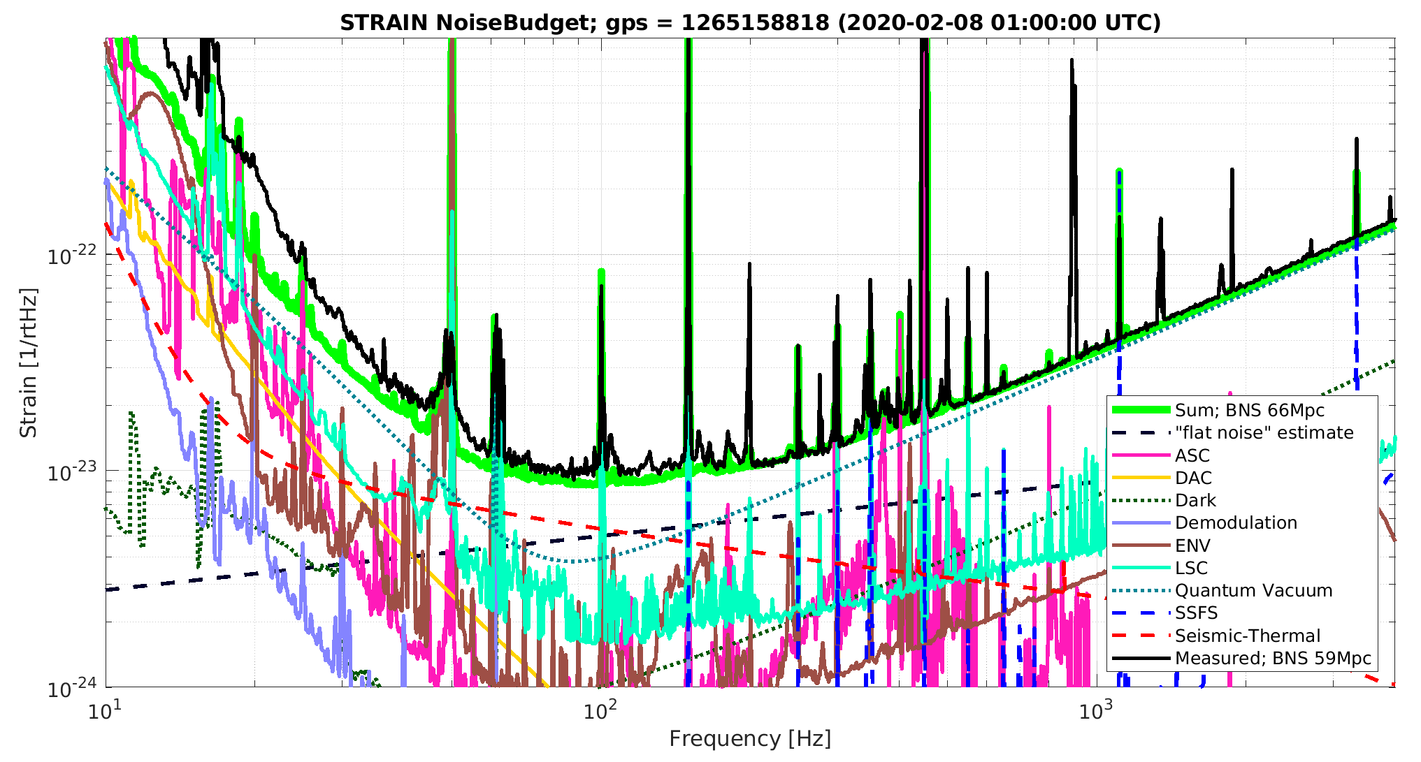
Figure 2: Snapshot of the adv O3 noise budget generated at a time of near best sensitivity of the detector (February 8th, 2020). The different noise sources shown are described in the text, the green line (bns range: 66 Mpc) represents the sum of these noises and it can be compared to the measured total noise shown in black (bns range: 59 Mpc).

ASC

– Angular Sensing and Control. This represents the control noise of 12 angular dof of the interferometer (two per mirror) and four dof of the beam injected into the interferometer. The coupling of these noises has been measured by injecting broadband noise into each dof [35].

DAC

– Digital Analog Converter. This is the electronic noise of the digital to analog converters used to drive the six main mirrors and marionettes of the interferometer. This electronic noise has been measured in the laboratory before installation, and the noise coupling is modeled using SimulinkNb.

Dark.

This is the electronic and dark noise of the photodiodes used in the four longitudinal dof control. The noise is measured by closing shutters of each photodiode, and the noise coupling is modeled.

Demodulation.

This is the phase noise of the demodulation of radio frequency signal from photodiodes to control carm, mich and prcl. That phase noise mixes the two demodulation quadratures. This bi-linear noise source is measured, and the noise coupling is modeled using SimulinkNb.

ENV

– Environment. This is the sum of three contributions: acoustic, magnetic and scattered light. The acoustic and magnetic noises are measured with four microphones and three 3-axis magnetometers, located in the experimental buildings near the interferometer components (see [29, 30] for details). Their couplings are measured by broadband and sweeping sine noise injections. Scattered light is measured in two ways: i) using the signal from auxiliary photodiodes which have a linear coupling that is modeled; ii) using position sensors of suspended benches that couple in a non-linear way modeled with a measured scaling factor [36].

LSC

– Length Sensing and Control. This represents the control noise of four dof: mich, prcl, omc length, and residual intensity noise. The noise is measured in all cases, the coupling is measured for all except for the omc length where it is modeled. Note that this results in double counting the dark and quantum noise of the sensors used for mich and prcl control, however these double counted contributions are negligible.

Quantum.

Quantum noise of the detector and shot noise of the sensors used for mich, prcl and carm control. The noise and the coupling are modeled using SimulinkNb.

ssfs.

This represents the control noise of the relative error between carm and the laser wavelength. The noise is measured, the frequency dependent coupling is modeled using SimulinkNb and a time dependent scaling factor is measured.

Seismic-Thermal.

This is the sum of the negligible seismic noise and three thermal noise contributions: suspension, mirror coatings and residual gas pressure in the arm vacuum tubes. The noise sources and the couplings are modeled using analytical functions in separate dedicated codes.

“flat noise”.

It is a noise source of not yet understood physical origin. Its level has been measured proportional to the square root of the darm offset used to obtain the interferometer DC readout [37, 38].

The sum of the noises described above correspond to a bns range of 66 Mpc, while the actual bns range in the corresponding data was measured at 59 Mpc. Hence, about 10% of the noise limiting bns detections is unaccounted for.

More in details, at frequencies above 1 kHz the sensitivity is mostly limited by quantum shot noise. The measured level is about 5% higher than expected. This is due to a slow degradation of the frequency independent light squeezing during O3, from 3 dB at the beginning of the run to about 2.5 dB at the end of it.

In the most sensitive frequency range, between 80 Hz and 200 Hz, there are significant contributions from three sources: quantum shot noise, mirror coating thermal noise and the “flat noise” of unknown physical origin. Assuming that the “flat noise” estimate is correct, removing completely this unknown noise source would have resulted in 10 Mpc improvement in the bns range.

At low frequencies between 20 Hz and 50 Hz, the dominant noise sources are quantum radiation pressure noise that is increased by the frequency independent light squeezing and the laser intensity noise. However 30% of the noise remains not understood in that frequency range, so other significant noise sources are yet to be identified.

3 The O3 run

The joint LIGO-Virgo Observing Run 3— "O3"— has been divided into two consecutive sub-data-taking periods, separated by a one-month commissioning break in October 2019.

• O3a: from April 1, 2019 at 15:00 UTC (GPS: 1238166018), to October 1, 2019 at 15:00 UTC (GPS: 1253977218).

• O3b: from November 1, 2019 at 15:00 UTC (GPS: 1256655618), to March 27, 2020 at 17:00 UTC (GPS: 1269363618).

All three detectors have participated to the whole run. The O3b end date has been anticipated by about a month, due to the worldwide covid-19 pandemic.

This section presents the LIGO-Virgo O3 run, seen from a Virgo perspective. First, we describe the main activities into which the data taking was divided, before summarizing how the detector was steered from the EGO control room. Then, we focus on actions taken to maximize the amount of data collected and to ensure their good quality. In particular, we highlight the main DetChar activities during O3, explaining how they fit and complement each other, following the flow of data from the detector to the final analysis. Key to achieve this level of performance and to maintain it over almost a year, were the 24/7 on-call duty service and the rapid response team: both are briefly described as well.

Then, we review the performance of the Virgo detector during O3, mainly from the point of view of the duty cycle. A high duty cycle requires not only a stable and robust detector against external disturbances (see [30] for a comprehensive study of that topic) but also a quick and reliable procedure to bring the instrument to its working point (the lock acquisition), starting from an uncontrolled global state. The main statistics of the Virgo O3 global control acquisition are thus provided, before studying the actual duty cycle. We also present the evolution of the adv detector sensitivity, from the O2 run to the end of O3.

This section ends with a brief overview of the final Virgo O3 dataset, describing how it was constructed offline, building upon the preliminary dataset estabilished by the live monitoring and data quality checks.

3.1 Data taking

While data acquisition was the highest priority during the O3 run, a limited fraction of the time had to be dedicated to other activities. The two main recurring ones were:

• the maintenance periods, held every Tuesday morning, staggered with respect to the similar times in LIGO, in order to maximize the two-detector network coverage. Maintenance, limited to about 4 hours per week, was used to look after the detector components, to perform various cleaning activities, and to host noisy activities incompatible with data taking— for instance the refilling of liquid nitrogen tanks located nearby the ceb, neb and web, delivered by heavy trucks.

• the calibration shifts, held almost every week on Wednesday afternoons or evenings. These campaigns allowed to check the accuracy of the reconstruction of the $h(t)$ strain stream [39], to monitor its stability over time and to test new, complimentary calibration methods, like the use of a Newtonian calibration [40] in addition to the usual photon calibrators [41].

In addition, commissioning time was allocated irregularly to tune or optimize some aspects of the detector, depending on the needs and opportunities. Finally, some time was spent studying and fixing problems impacting the data taking.

3.2 Detector steering

The Virgo data taking is largely automated and usually only requires a single operator on duty in the control room. Operators are present 24/7 during a run and take shifts every 8 hours.

The adv detector automation, called Metatron, relies on the Guardian [42, 43] framework, developed by LIGO and based on hierarchical finite state machines. The Virgo implementation links this framework to the daq: automation nodes become daq nodes that get data directly from shared memories and are synchronized with the one-second data availability period. A generic mechanism to read and write daq channels has been introduced and can be used within user codes via dedicated functions.

The full Virgo control acquisition procedure has been implemented in Metatron, initially prior to the O2 run and then updated for the O3 configuration—the main difference being the addition of the frequency-independent squeezing [26]. The scheme adopted, depicted in Figure 3, strictly follows a bottom-up approach, with the lower-level nodes being automatically managed by higher-level ones.

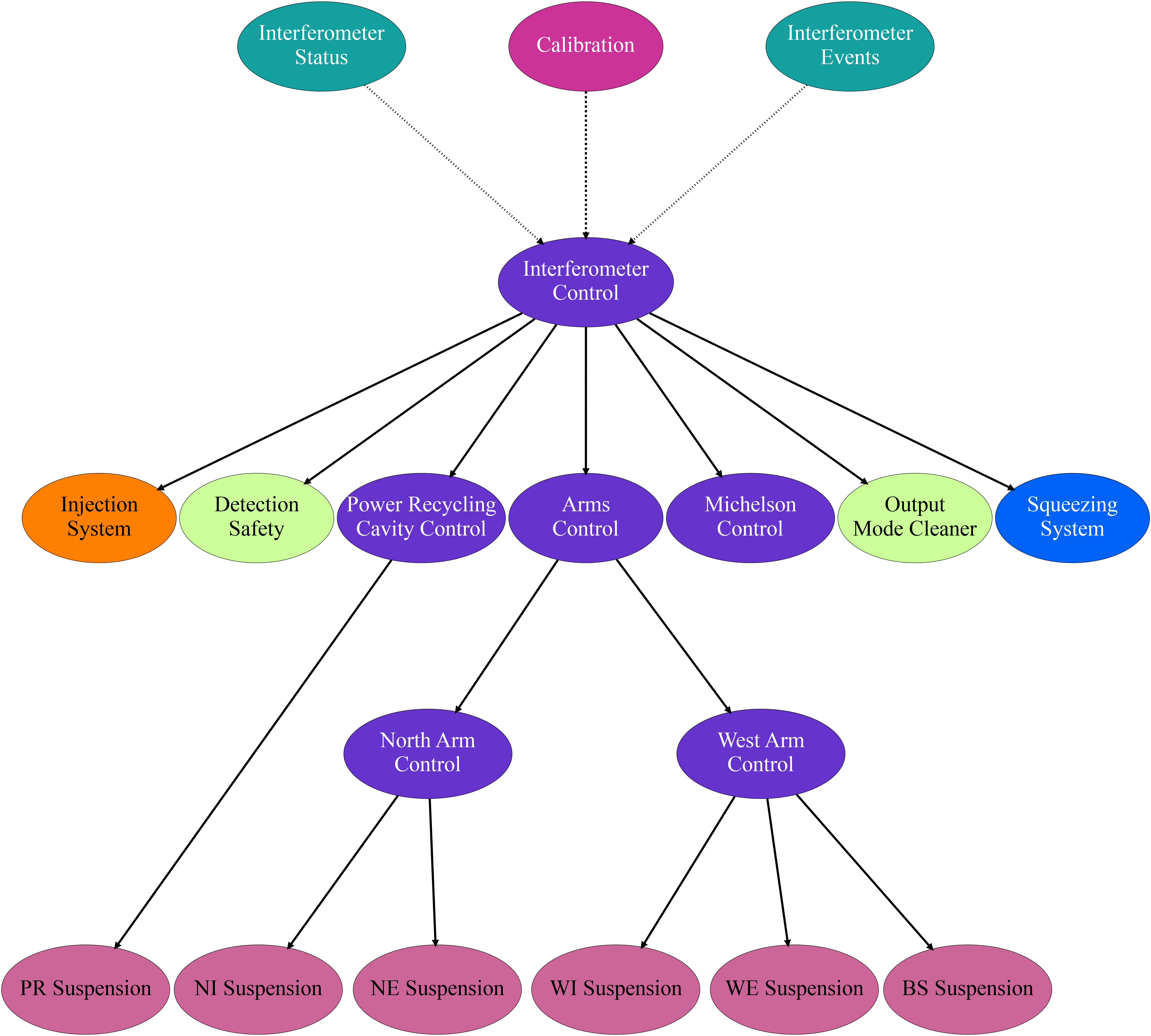
Figure 3: Metatron nodes hierarchy used during the O3 run.

The suspension nodes (violet background in the graph) are tasked to align/misalign the Virgo optics; each of them is managed by the most appropriate control nodes (dark blue background), divided on the basis of the degrees of freedom to be controlled. The main node—Interferometer Control— is usually the only one operated manually to steer the detector. It defines the control paths such as for instance the main global control procedure that allows reaching the Science mode (the nominal data taking state), plus other procedures to control various configurations of the optics or to perform automated calibrations, etc. It relies on the underlying managed nodes to perform these actions on the instrument. During the final steps of the control procedure, each single part of the interferometer is ultimately entangled with the others, and the interferometer is naturally treated as a single system; for these reasons, the last part of the procedure is directly managed by the upper level node, which sets the control parameters to the whole system, while the lower level nodes are only used as watchdogs for the correct functioning of their own sub-systems.

Additionally, the Metatron main node manages:

• the laser Injection System, from the laser source to the imc (orange background);

• the two Output Mode Cleaners that are controlled in sequence in the final steps of the nominal control acquisition procedure (pale green background);

• the Detection System at the interferometer output port (pale green background);

• the frequency-independent Squeezing System (light blue background), whose control proceeds in parallel to the main detector control procedure. As Virgo can take valid Science data with or without this system being in its nominal state, the corresponding Metatron node is a bit apart from the others logic-wise.

Only during the calibration measurements, the Interferometer Control node is automatically managed by the Calibration node (magenta background).

The Metatron framework also takes care of generating high-level flags that provide the overall status of the interferometer: this is done within the Interferometer Status node (dark green background). Finally, the Interferometer Events node (dark green background) records all state transitions of the detector. The Interferometer Status and Interferometer Events information is passed onto the Virgo live monitoring system, documented in Section 4.1.

3.3 DetChar organization

Figure 4 shows the flow of data, from the interferometers (IFOs, on the left), to the physics analyses (on the right). While focusing on the gw candidates, this schematic highlights the three main pillars of DetChar activities during a run.

• The first timescale on which DetChar activities take place is online (latency: $\mathcal{O}(\textrm{s})$). Quick automated checks are run on live data to mark out (good or bad quality) the data stream used as input by the “pipelines”—that is the algorithms that scan the network data in real time, as soon as they become available. Initial data quality information is indeed shipped alongside the reconstructed gw stream, as explained in Section 5.

• The second timescale is near real-time (latency: $\mathcal{O}(\textrm{min})$), crucial to assess the quality of the gw candidate public alerts. Thanks to a dedicated framework that is described in Section 6, the data around a significant candidate are vet for each detector and a global decision is then taken: either to confirm the public alert sent to the telescopes or to retract it (see Section 3.4 below for a description of the procedure).

• Finally, the last timescale is offline (high latency: up to months after the data taking). The goals of these studies are twofold: first, to finalize the dataset that all offline analyses will use, regardless of whether they look for transient or continuous signals; then, to validate the events that will be included in the final publications and whose parameters will be used to extract astrophysical information.

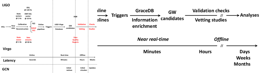
Figure 4: Dataflow from the interferometers (labelled "IFOs" on the left) to the offline validation of gw candidates and the completion of the final dataset (right). It focuses on the generation and the vetting of the public alerts that are a key product of the LIGO-Virgo observing runs. It shows the three main timescales at which the Virgo DetChar group operates: online, near real-time and offline (see text for details).

To ensure a continuous monitoring of the data quality, DetChar shifts were organized during the entire O3 run on a weekly basis, with two people (working onsite or remotely) on duty. The shifter crew changed every Tuesday morning, during the weekly maintenance of the Virgo detector. In addition to attend all relevant meetings. DetChar shifters usually reported their findings at the weekly DetChar meeting on Fridays and at the weekly detector meeting on Tuesdays (thus at the end of their weekly shift).

3.4 On call duty service and rapid response team meetings

An on-call service was organized during the O3 run to ensure a 24/7 expert coverage for all the Virgo detector components, from hardware systems to online computing and DetChar. In case of a problem, the operator on duty would contact the relevant experts from the control room, plus the data taking coordinators if needed.

In addition, a joint LIGO-Virgo low-latency automated alert system was setup to contact the rrt experts—specialists of data taking, data quality or gw transient searches—that would meet remotely on short notice each time a public alert candidate had been identified in real time. They would vet that candidate, using all raw information available, plus the output of several data quality checks, triggered automatically by the generation of the signal candidate: the dqr, see Section 6.1 for details. The outcome of an rrt meeting could be twofold: either to confirm the public alert, or to retract it when the astrophysical origin of the candidate was questionable.

3.5 Virgo O3 duty cycle

Table 1 summarizes the performance of the global control acquisition procedure for the Virgo detector during O3. This performance has been stable over the whole run, showing the robustness of that procedure. As not all control acquisition attempts are successful, a global control acquisition procedure is defined as a set of successive control attempts that leads to the global control of the instrument.

The median duration of a successful global control acquisition attempt is 18 minutes: about 30% of this time is spent reaching the detector working point (Michelson interferometer at the dark fringe, power recycling cavity and arm cavities resonant, ssfs enabled); 50% is spent to control the two omc at the Virgo output port; the final 20% are used to reach the lowest noise configuration at the level of the suspension actuation.The median number of attempts needed to complete a global control sequence is 2 and the median duration of a successful global control acquisition sequence is 25 min, during O3 the quickest sequence took about 13 min.

Table 1: Summary of the Virgo global control acquisition performance during O3: the control is acquired after a successful control acquisition sequence that counts one or more control acquisition attempts.

Global control acquisition attempt
	Median duration	18 minutes
	Distribution of this time
	Reaching the detector working point	${\sim}$30%
	Controlling the two omc	${\sim}50$%
	Acquiring the lowest noise configuration	${\sim}20$%
Global control acquisition sequence
	Median number of attempts	2
	Median duration	25 min

Table 2: Summary of the O3 data taking performance of the Virgo detector. The last three rows of the table provide duty cycles for different configurations of the 3-detector LIGO-Virgo global network: the fraction of the time during which at least one the three instruments is taking data, at least two are and finally all three are.

		O3a	O3b	O3
Virgo global control segments	Mean [hr]	6.1	6.4	6.3
	Median [hr]	2.7	1.8	2.2
Virgo Science segments	Mean [hr]	5.0	4.0	4.5
	Median [hr]	2.6	1.4	1.9
Duty cycles	Virgo [%]	76.3	75.6	76.0
	Network—at least 1/3 [%]	96.8	96.6	96.7
	Network—at least 2/3 [%]	81.9	85.4	83.4
	Network—3/3 [%]	44.5	51.0	47.4

Table 2 details the control stability of the Virgo detector, separately for the sub-runs O3a and O3b, and averaged over the whole O3 run. The “global control segments” are stretches of data during which Virgo is controlled in its nominal low-noise configuration, while the “Science segments” are the subset of the global control segments during which Virgo is taking data of good, science-compatible, quality. The difference of duration between the global control and Science segments is dominated by limited disruptions of the data taking, that usually stop the Science mode for a short time. The dominant source of these breaks is the frequency-independent squeezer that lost its nominal configuration about 240 times during the O3 run; the median time to restore it and switch back to Science data taking was about 140 seconds.

We note that the Virgo segment duration summary numbers listed here are lower than those reported by LIGO [44, 45]. Yet, this difference has no significant impact on the duty cycle that is very similar for the three detectors of the global LIGO-Virgo network. The comparison between the O3a and O3b sub-runs shows that the impact of the winter season (larger sea seismic activity, wind, and more generally bad weather), although real, has been limited. Overall, the global network duty cycle has improved during O3, mainly due to the increase of the LIGO detectors duty cycle, while the Virgo one has been very stable. With an average of 76%, the Virgo O3 duty cycle is lower than that measured during August 2017, the final weeks of the O2 run Virgo took part of: ${\sim}$85%. Yet, the O3 performance has been achieved over 11 months spanning a whole calendar year and cannot be directly compared to the duty cycle of a 25-day run in Summer time, the most favorable period to operate an instrument like Virgo. Running one full year instead of one month is also more complex person-power wise, and the Virgo organization implemented during O3, although perfectible, held on during the whole run. This experience represents a good base on which to build upon in order to improve the Virgo performance for the O4 run and beyond.

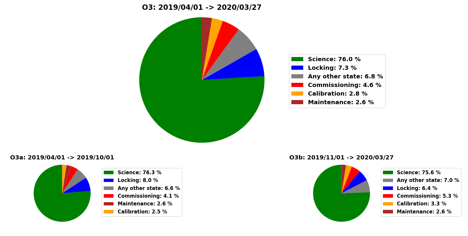
Figure 5: Breakdown of the time spent in different modes by the Virgo detector during the O3 run (larger, top-middle pie chart) and separately during the O3a and O3b sub-runs (pie charts at the bottom). The Locking mode corresponds to periods when the control of the detector is being acquired. The regular maintenance and calibration periods have been described in Section 3.1. Finally, the Any other state category includes all the other situations encountered during the whole run: troubleshooting periods, various kinds of tuning, etc. These results exclude the 1 month-long commissioning break that took place in October 2019, in between the O3a and O3b sub-runs. In each pie chart, the modes are sorted by decreasing percentage.

Figure 5 shows the breakdown of the time spent in different modes by Virgo during O3. Overall, the O3a and O3b distributions are quite consistent. Breaking these 11 month-averaged duty cycle figures down to a 24-hour period, Virgo took data during about 18 hours, with the remaining six hours roughly divided into three blocks of the same duration: ${\sim}2$ hours for controlling the detector (Locking), ${\sim}2$ hours for recurring activities (Calibration, Commissioning and Maintenance) and ${\sim}2$ hours for solving issues (Any other state).

The analysis of these pie charts shows that increasing the duty cycle during future runs will not be straightforward. The room for improvement is limited in each area and so any significant duty cycle gain will likely stem from a combination of various small progresses, each made possible by the redesign or the optimization of a particular process.

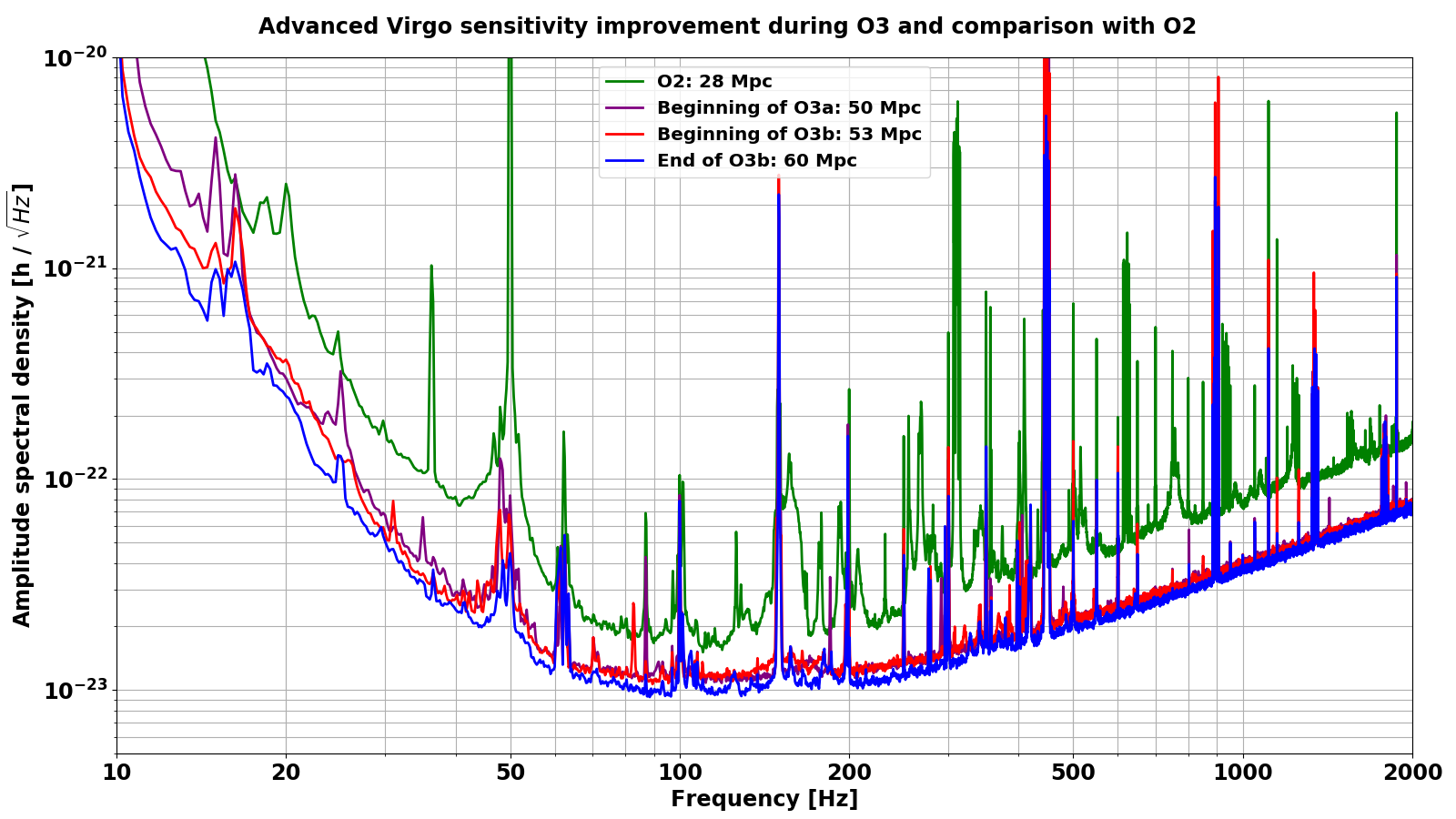
Figure 6: Comparison between four sensitivity curves of the adv detector: during O2 (green trace), at the beginning of O3a (purple), at the beginning of O3b (red) and at the end of O3b (blue). The caption provides the corresponding estimated bns ranges.

To conclude this overview, Figure 6 summarizes the improvement of the sensitivity of the adv detector. The bns range associated to each curve is given in the legend. From O2 to O3b, the bns range has more than doubled from 28 to 60 Mpc, with a continuous improvement of the sensitivity in the whole bandwidth of the detector. Many spectral features of the residual noise structures have either been removed or significantly reduced over time.

3.6 The Virgo O3 dataset

The final Virgo O3 dataset consists of more than 250 days of data recorded during the O3a and O3b sub-runs and whose quality has been checked and validated (described in Section 7.4.1). It is built upon and supersedes the online good-quality Science dataset that was used as input by the analysis pipelines that looked for gw in real time (see Section 5). Dedicated studies have been performed offline to refine the quality assessment of the data. In addition to running more in-depth analyses, new checks have been added during the run, as potentiel flaws got discovered in the existing analyses, or new problems identified at the detector level. Moreover, small sets of good data that had not been automatically included in the dataset (either because they were incorrectly labeled or because part of their data quality information was missing) were added by hand.

The main categories of checks applied to assess the quality of the Virgo data are the following.

• Are key components of the Virgo hardware (suspensions and photodiodes) having transient problems?
  These checks, described in Section 5.1.2, were fast enough to be performed online on live data.

• Is the reconstruction of the gw strain time series $h(t)$ nominal?
  This is a prerequisite for any further use of the Virgo data. The online reconstruction of the Virgo data was satisfactory: only about three weeks at the end of O3a were reprocessed offline to increase the sensitivity by a few percents [39]. Yet, during periods of high seismic activities (bad weather, high wind or the passing of seismic waves from strong and distant earthquakes), it could be replaced [30]) by a more robust control configuration— the so-called "earthquake (EQ)-mode" [39]. Although that procedure saved some lock losses whose recovery would have costed time, it could not be validated against the nominal reconstruction of the $h(t)$ strain stream until the final two months of O3b. Therefore, during most of the O3 run, data taken in these peculiar conditions had to be excluded from the final dataset.

• Do the data suffer from known problems?
  Tailored checks were run offline to identify and isolate periods during which the detector was not behaving nominally, although it was still controlled.One example of such studies is the fact that the North Input mirror suspension was randomly suffering from a transient (a few second-long) loss of data. This was usually enough to lose the control of the entire detector, and hence to lose at least about 20-30 minutes of data: the time to reacquire the locked state and to restore Science data taking. Therefore, a patch was developed by experts to detect the data loss and switch to a less robust—but still available—control until the missing data were back. This saved hours of running time for Virgo overall, but a dedicated scan of the data had to be performed offline to identify the occurrences of these control switches (potentially inducing transients and artifacts of instrumental origin in the data) and to remove them from the final dataset.

• Are the data consistent?
  For instance it was decided to remove offline the last few seconds of a segment preceeding a control loss of the detector as those data could be corrupted— see Sec. 7.4.1 for details

• Is the dataset complete?
  For example there could be segments with missing or corrupted $h(t)$ channel that would require a limited reprocessing. Or there could be segments with missing missing data segments due to problems in the DAQ, etc..

Data segments that fail one of the checks defined above are classified as "Category 1" (CAT1) vetoes and must be excluded from all analyses. Overall, only about 0.2% of the Virgo O3 Science dataset have been CAT1-vetoed.

To conclude this overview of the Virgo performance during the O3 run, Figure 7 compares the Virgo bns range distributions before (red) and after (blue) applying data quality cuts to determine the final O3 dataset. As expected, data quality requirements remove periods of low bns range, i.e. when the sensitivity was poor. Yet, about 1% of the data have a bns range lower than 35 Mpc, that is significantly below the typical values achieved during O3 for that sensitivity estimator. While these data have not been flagged as bad by the various checks run on the dataset, they correspond to periods during which the detector was less accurately controlled, in particular due to bad weather.

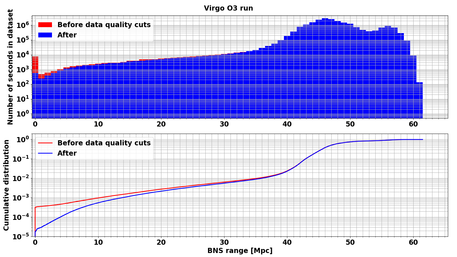
Figure 7: Distributions of the Virgo bns range during O3 for the online (red histogram and trace) and offline (blue) dataset. The top (bottom) plot compares the histograms (cumulative distributions).

4 Tools for detector characterization and data taking monitoring

All DetChar analyses rely on dedicated software frameworks, called generically tools in the following. Most of these have been developed within Virgo. In addition, thanks to the long-lasting collaborations among the Virgo, LIGO and now KAGRA DetChar groups, we benefit from additional tools or methods that have been developed partly or totally by colleagues.

More than 100 servers have been running in real-time during O3 to monitor the Virgo detector, run various data quality checks and perform specific DetChar tasks. Data are processed by the tools described in the following subsections and whose outputs are included in the live data streams or stored on disk. Finally, the end products of these analyses are converted into information for the control room and summary plots that are updated with a latency of a few minutes at most and regularly archived for offline analyses.

All these processes are steered using the vpm software interface, that allows to configure, start/stop and monitor processes running on Virgo online servers. These include detector control, data transfer to and from Virgo, and the analysis of the reconstructed $h(t)$ stream by the online gw searches running in the EGO computing center. All actions performed using the vpm interface are logged and recorded, in order to reconstruct as accurately as possible the software running at any given time, should this need arise.

The most important DetChar tools used during the O3 run are described in the following. They have been classified in a few categories depending on their usage or target: monitoring, generic data analysis, glitches, spectral noise or databases. Yet, they are not independent: they are often combined to characterize some features of the detector, or to provide a complete overview of the quality of the Virgo data. The flowchart in Figure 9 represents the main analyses carried out by the DetChar group with the tools presented in this section. The arrows follow the data-flow, which starts from the detector raw data that is analyzed by the various tools, whose data products are then saved to disk and used to generate DQ flags and reports. The latter are used by both GW search pipelines and by commissioners and operators that control the status of the detector.

Figure 8 describes a specific example of joint application of various analysis tools and monitors to the study of transient noise.

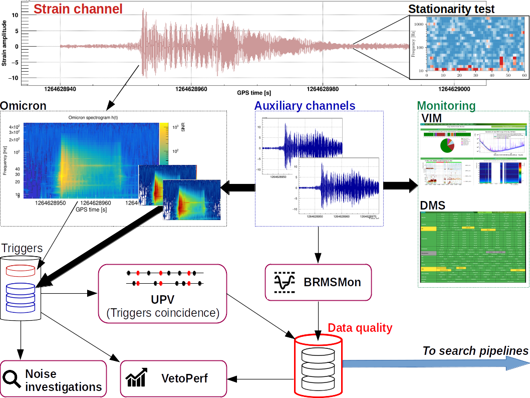
Figure 8: The Virgo strain data and auxiliary channels are analysed by DetChar tools to monitor and investigate transient noise. The noise stationarity is monitored with dedicated tools (Section 4.2.3). The data is analysed with Omicron (Section 4.3.1) and transient triggers are saved to disk for further noise investigation. In particular, the UPV algorithm (Section 4.3.2) isolates coincidences between triggers from the strain and auxiliary channels. BRMSMon (Section 4.2.2) detects transient noise excesses in axiliary channels. Both UPV and BRMSMon generate data quality segments used to reject transient noise found by GW searches. The performance of these data quality segments is evaludated by a tool called VetoPerf (Section 4.3.3). The transient noise is also monitors with web tools like VIM (Section 4.1.3) and the DMS (Section 4.1.2).

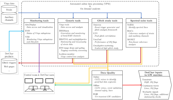
Figure 9: Flowchart of the various tools and monitors used for detector characterization that are presented in Section 4. The data-flow starts from the raw data acquired from the detector, which is analyzed by the various tools and used to produce processed data and data visualizations used for monitoring purposes. Some of the outputs of the various tools are used to generate DQ products, to be used by GW search pipelines and commissioners to control the interferometer.

4.1 Monitoring tools

4.1.1 dataDisplay

The dataDisplay software [46] allows the user to read (online or offline) Virgo data and to visualize various types of plots for all the channels available from the DAQ. For instance, it helps to investigate quickly the time evolution of a noise artifact, the coherence between two control signals or the time-frequency characteristics of a transient noise. It has been used extensively during the O2 and O3 runs and all over the adv detector commissioning in between. Figure 10 shows an example of the dataDisplay interface and output.

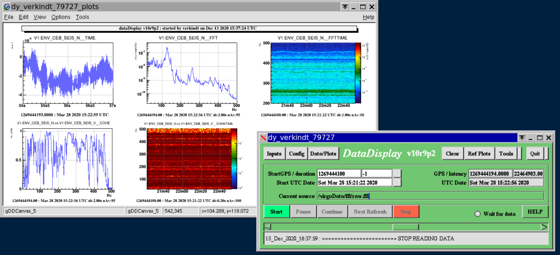
Figure 10: Example of the plots produced by the dataDisplay (left) and main panel of the dataDisplay graphical user interface (right).

4.1.2 DMS: the Detector Monitoring System

The dms [47, 48] provides a detailed live status of all the components that make the Virgo detector operate, from the hardware parts to the online software used to control the instrument and take data. It also includes the monitoring of environmental data from around the experimental areas. Each of the many dms monitors uses a set of daq channels, combines them by performing mathematical and logical operations on their outputs and produces a flag whose value can take four severity levels, each associated with a color for visual display. A web interface is used to display and browse the dms monitor flags with a few second-latency, both in the Virgo control room and remotely.

In addition, a new dms archival system has been set up for the O3 run: complete dms snapshots are taken every ${\sim}10$ seconds and archived. They can be retrieved later at any time, by running a playback application that uses the same interface as the live dms. This functionality is particularly convenient to check the status of the detector a posteriori, when a gw candidate or a particular feature in the data have been identified. For instance, Figure 11 shows the Virgo detector status about four seconds after the detection of the gw event GW190412 [49].

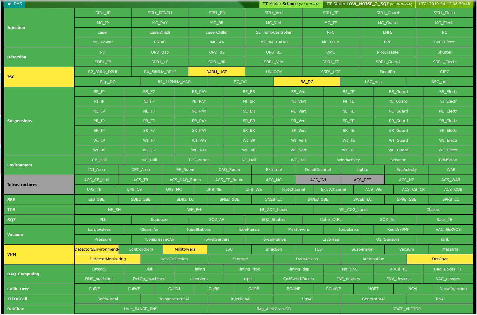
Figure 11: DMS snapshot closest in time to the GW190412 gw event, showing the detailed status of the Virgo detector about four seconds after the arrival of that signal. The DMS web interface looks like a checkerboard. Each row, labelled in the most-left column, corresponds to a different part of the instrument (mirror suspensions, vacuum system, etc.). That part is broken down in smaller sets that are each associated with a cell on the web interface. Each cell can contain many DMS flags and its color reflects the highest severity among all these flags (green $\leftrightarrow$ no alarm; yellow $\leftrightarrow$ warning; red $\leftrightarrow$ alarm (not present on that particular snapshot); grey $\leftrightarrow$ some information is missing). Clicking on a cell gives access to the flag individual information: their values and associated severities.

4.1.3 VIM: the Virgo Interferometer Monitor

The vim [50, 51] manages a collection of automated scripts that update every few minutes a wide set of plots and tables; all these monitoring products are archived on a daily basis. A web interface allows users to browse that database, both for live monitoring of the experiment and for offline investigations. vim is an essential tool that provides a direct access to a detailed status of the various Virgo detector components and of related frameworks, such as calibration and online data processing, data transfer or online data analyses. A snapshot of the vim web interface is shown in Figure 12.

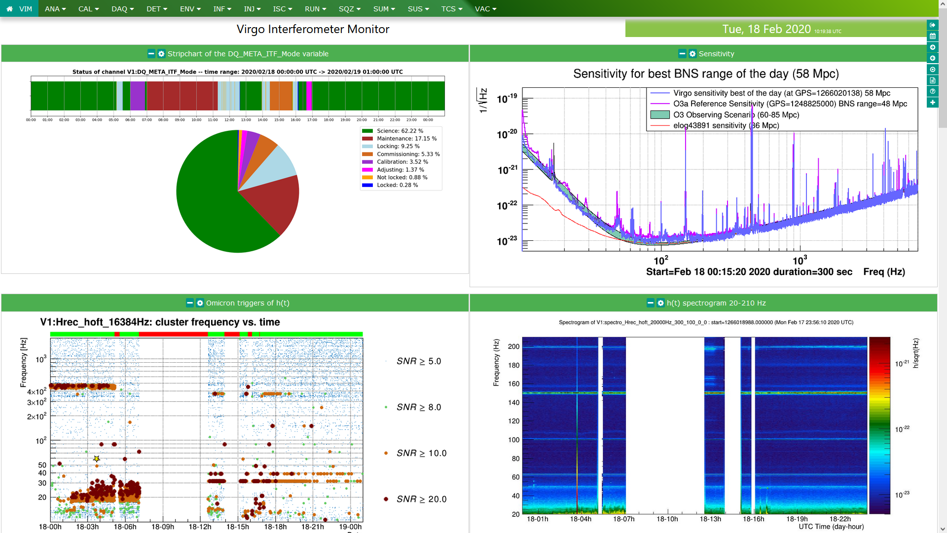
Figure 12: Screenshot of a vim webpage displaying information about the Virgo detector on Tuesday February 18, 2020. Top left plot, stripchart of the detector status: the weekly maintenance, preceded by a planned calibration and followed by a short commissioning period, interrupts the data taking that restarts in the evening. Top right plot: daily sensitivity compared with references. Bottom left plot: glitch monitoring provided by the Omicron analysis described in Section 4.3.1. Bottom right plot: spectrogram of the gw strain $h(t)$ in the 20-210 Hz frequency range.

4.2 Generic tools

4.2.1 The VirgoTools utilities

In-depth studies of a particular feature observed in the data or analyses scanning a significant fraction of the dataset require the use of dedicated software. Common and key building blocks of these codes are access to the daq channels and to the detector component configurations. Thus, dedicated packages have been developed over the years to provide simplified and generic interfaces to these data: they rely on low-level core packages like the FrameLib software library [52] but calls to these functions are hidden to the users. These packages interact with the software, hardware and data of the Virgo interferometer: they are widely used within the collaboration, from daily use in the control room to DetChar studies. The two main collections of such functions are PythonVirgoTools [53] and MatlabVirgoTools, targeting Python and Matlab developers respectively.

4.2.2 Computing Band-limited RMS

brms of daq channels in specific frequency ranges are useful indicators for transient disturbances or new features in the data. For instance, low-frequency brms of seismometer data allow to separate different contributions to the seismic noise at EGO [30]. Going from low to high frequencies, one can isolate successively: distant and potentially strong earthquakes; sea activity on the Tuscany coastline; anthropogenic contributions with day/night and weekly periodicities; finally, on-site activities. In addition, brms are used to monitor the excitation of the violin modes, the resonances of the mirror suspensions.

In Virgo, various software frameworks can compute brms. One worth-mentioning is BRMSMon, a dedicated software that is widely used by the environmental monitoring team and in data quality studies. In addition to generating brms, BRMSMon can compare their values to thresholds (either fixed or adaptive) and logically combine the outputs of these comparisons into binary channels called flags. For instance, assuming a collection of 9 sensors installed in different EGO buildings, one can create a flag that is active (value equal to 1) if at least 5 of these 9 sensors exceed their own threshold and inactive (value 0) otherwise. The BRMSMon output channels, sampled at 1 Hz, are included in the DAQ.

4.2.3 Testing stationary and Gaussianity

Several analysis tools have been implemented to perform statistical tests to verify the stationarity and Gaussianity of the data. These properties are indeed the typical assumptions at the base of most of the statistical analyses, and in particular of the matched filter technique [54, 55], which modeled gw searches such as MBTA [56], PyCBC [57] and GstLAL [58] are based on. Moreover, the onset of a non-stationary behavior of the detector can be the symptom of some hardware malfunction or some contamination from environmental noises. In any case, it requires prompt investigations of the causes and, possibly, the actuation of adequate mitigation strategies.

bristol provides a multi-band stationarity test based on the empirical distribution of the signal brms [59]. Stationarity is tested dividing these brms’ into chunks and verifying the compatibility of their empirical distribution functions by means of a two-sample Kolmogorov–Smirnov test [60]. This provides $p$-values that, compared to a previously decided significance level, indicates where in a time–frequency map the hypothesis of stationary should be rejected. The resolution of this map is given by the duration of each chunk and that of the brms estimates, typically one minute and one second respectively; that in frequency is determined by the band division of the spectrum for computing the brms’, which is conveniently done choosing exponentially spaced frequency intervals. The typical output of this tool is reported in Figure 13, while further details about the definition of the test statistic are discussed in A.1.

bristol mainly targets slow non-stationarities, that is, changes in the statistical properties of the data over time scales longer than a second; for faster transients, namely glitches, other strategies are typically used and will be described in Section 4.3.

This tool has been developed in the commissioning phase preceding O3, and has been used during the run to assess the quality of the data as part of the event validation procedure (refer to Section 7.4.2 for more details).

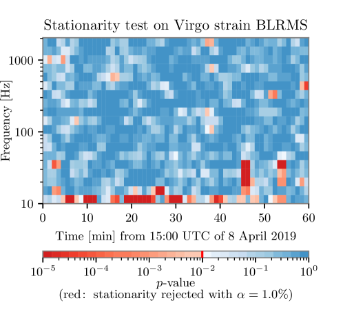
Figure 13: Example of stationarity time–frequency map obtained with bristol, where a significance $\alpha=1\%$ has been chosen and regions rejecting the stationarity hypothesis are colored in shades of red.

rayleighSpectro [61] is a tool to test the hypothesis of Gaussianity of the data at each frequency of its spectrum. This is based on the Rayleigh test [62], which is a consistency test of the asd estimates on various data intervals.

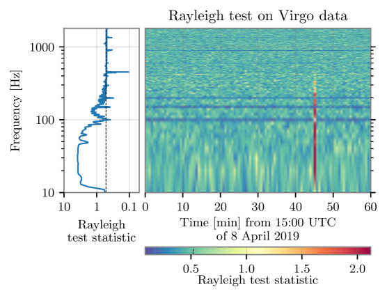
Figure 14: Example of application of the Rayleigh test, where the blue line in the left panel is the test statistic estimated over the entire hour of data, while the colormap corresponds to asd estimates over $10$ seconds of data. The vertical black line on the left plot indicates the limit value 0.52. See text for details.

If the data is stationary and Gaussian, the asd estimate is drawn from a Rayleigh distribution at every frequency, and the ratio of its standard deviation and mean should be asymptotically equal to

$$\frac{\sqrt{4-\pi}}{\sqrt{\pi}}\simeq 0.52$$ (1)

That constitutes the test statistic. Deviations from this value can be both a symptom of asd misestimation, due for example to non-stationary data, or to regions of the spectrum where the data is not compatible with a Gaussian distribution, as for example regions corresponding to spectral lines. More details about this test are presented in A.2.

This tool can be used complementary to bristol to independently test stationarity and Gaussianity. It is included in vim and also used in the dqr for event validation (see Sections 4.1.3 and 6).

Figures 13 and 14 show examples of application of these two tools to one hour of data at the beginning of O3a. In the former, bristol highlights many slow non-stationarities at frequencies up to about $20~{}\mathrm{Hz}$, most likely due to high microseismic activity, as well as a loud glitch at about 15:45 UTC. The latter is clearly identified by the Rayleigh test with values of the test statistic larger than what is expected for stationary and Gaussian noise. Moreover, in the colormap of Figure 14, spectral lines, in particular those associated with the $100$, $150$ and $200~{}\mathrm{Hz}$ harmonics of the mains (the European power grid frequency is 50 Hz), are highlighted in blue, corresponding to values of the test statistic smaller than the reference one of Equation (1). In the left-hand side panel of the same image, the $450~{}\mathrm{Hz}$ frequency of the main test masses violin modes, and its first harmonic at about $900~{}\mathrm{Hz}$, are highlighted as well.

Figure 15 shows another example of a Rayleigh spectrum around an O3b time where transient noise was present for several minutes between 10 Hz and 20 Hz.

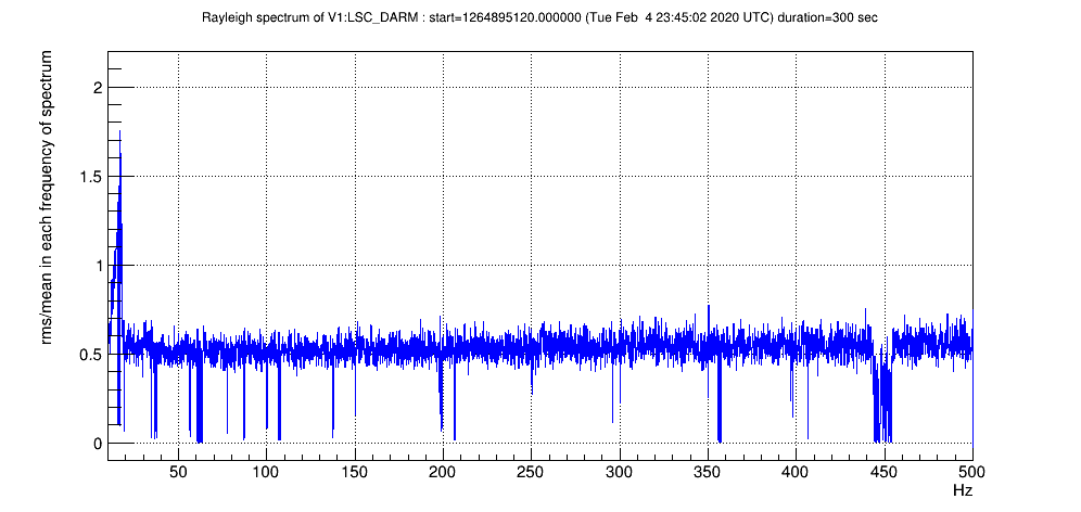
Figure 15: Example of Rayleigh spectrum averaged over 300 s, where any bin above 0.52 is a potential non-stationary or non-Gaussian noise present during those 300 s. Values well below 0.52 correspond to persistent frequency lines.

4.2.4 Monitoring BNS range drops and gating data

Two useful high-level data quality monitors are based on bns range downwards excursions: one tags bns range drops, that are significant dips in that quantity, while the other automatically generates (logical) gates that are applied on the gw strain channel to smooth out to zero the data that are affected by a strong noise transient.

bns range drops

A bns range drop means that the live sensitivity of the detector is degrading significantly, at least in a given frequency band, possibly in the entire bandwidth of the instrument. Therefore, it is important to identify transient sensitivity worsenings and investigate their causes. bns range drops are very diverse: the decrease goes from a few percents to almost the full range, while the drops can last from a few seconds to minutes.

During O3, bns range drops were detected using an absolute threshold on the live value of that quantity. After the end of the run, adaptative methods able to follow the natural evolution of the bns range and to locate all significant drops have been developed. Figure 16 shows examples of the output of the adaptative bns range drop locator running on O3 data.

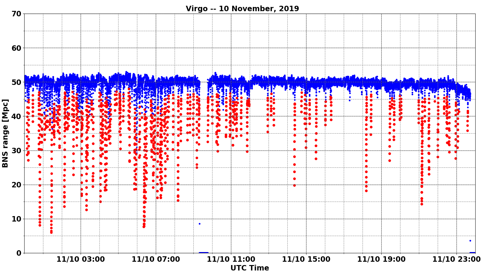
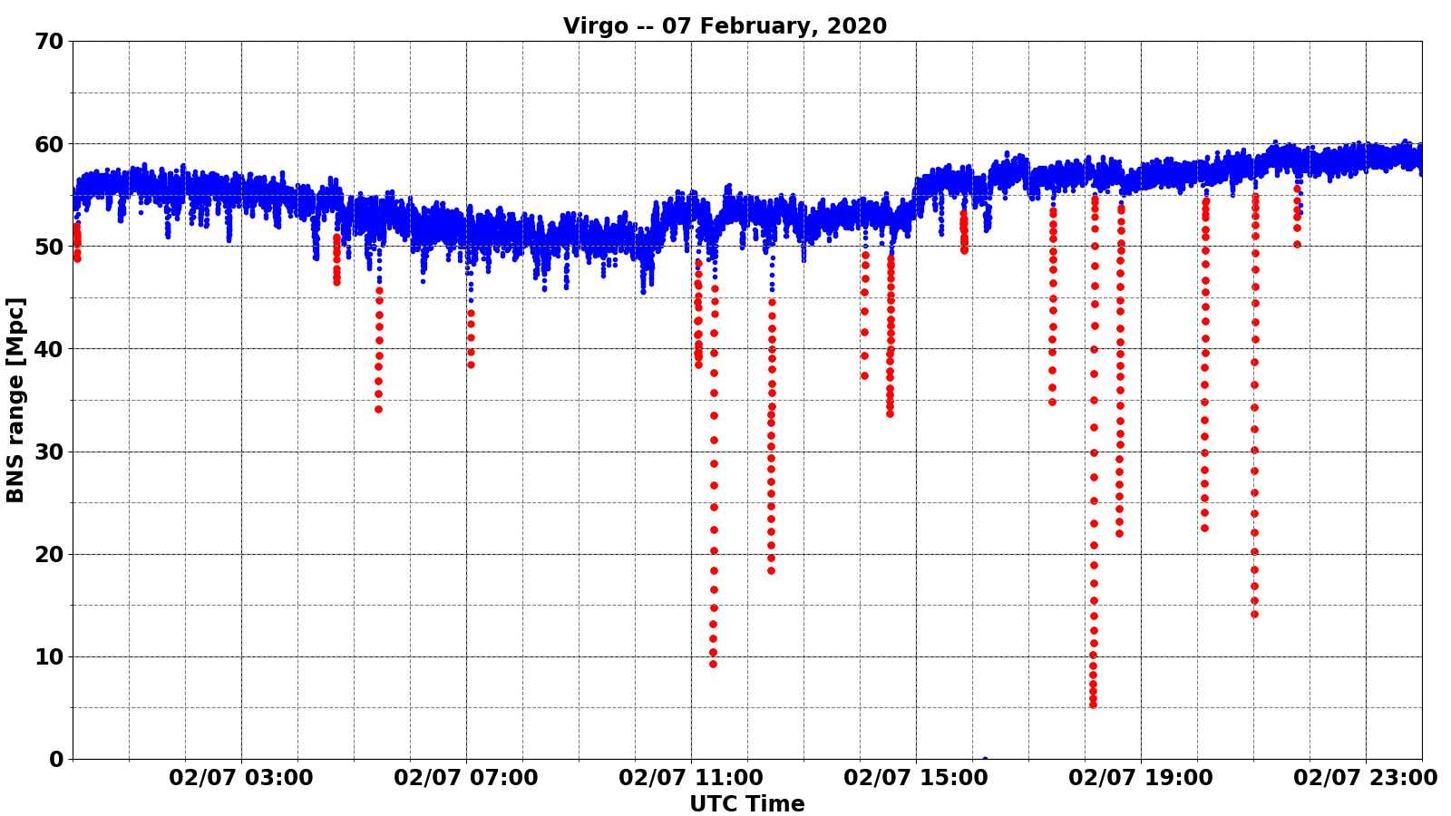
Figure 16: Performance of the bns range drop locator during two days of O3. Top plot: November 10, 2019, a day during which the duty cycle was quite high but the data taking conditions were not stable; many glitches and consequently bns range drops were observed, mostly due to the laser power stabilization system in the morning and to a worsening of the weather conditions starting from the afternoon. Bottom plot: February 7, 2020, a day with no global control loss but a bns range baseline varying over time; actions took place during the afternoon to improve the Virgo performance, leading to visible improvements of the bns range in steps. The blue traces show the range vs. time, while the red dots show the drops that have been identified. In both cases the bns range drop locator is able to identify most, if not all, significant drops.

Gates

If not removed from data, noise bursts can pollute the estimation of the noise spectrum for several seconds, hence limiting the sensitivity of the gw search algorithms during that period. In Virgo, this problem is mitigated online by gating out (meaning zeroing) glitchy chunks of data. The gating algorithm triggers on significant bns range drops: at least 40% below its median value, computed over the last 10 seconds. On both sides of the gate, a weight is applied on the $h(t)$ strain channel during 10/32^th of a second, varying smoothly from 1 to 0 (0 to 1) before (after) the gate. The online gated $h(t)$ strain channel is included in the DAQ alongside the ungated one and GW searches are free to use one or the other stream as input.

As gating is based on $h(t)$ variations, gated data cannot simply be removed from the physics-analysis dataset as this procedure could flag real gw, for instance loud high-mass binary black hole mergers. On the other hand, gating information can be used in a statistical way to help identify potential periods of bad data quality characterized by frequent gating usage. This can be measured using both the density of gates (number per time unit) and the fraction of the wall-clock time that is gated out.

During O3, the gating algorithm has produced more than 13,000 gates (corresponding to a few tens per day in average), adding up to about 4 hours of gated data in total. The gate mean duration is around 1.1 s while the median is around 0.8 s, meaning that most gated glitches are very short as 20/32^th s are always added to the measured glitch duration to transition from non-gated data to the gate itself and back. The longest gate is about 10 s.

Excluding from this online Science dataset the segments that have been vetoed for offline data analyses (see Section 3.6) leads to a removal of about 20% of the gates and of about 30% of their total duration—although this procedure only removes about 0.2% of the Virgo O3 dataset. As expected, gates are most likely when the data are bad. Going one step further by requesting in addition that the baseline bns range be greater than 35 Mpc, one excludes more than 50% of the remaining gates and more than 60% of the gated times while that cut would remove about 1% of the data from the final dataset. Gates are generated more often when the data taking conditions are sub-optimal.

Finally, one can associate all gates with a glitch detected by Omicron (see Section 4.3.1) whereas the opposite is not true: there are many glitches that have no impact on the bns range. These glitches have a frequency range that is outside of the Virgo bandwidth for bns gw waveforms: either because there is no significant signal contribution expected in this frequency range, or because the noise level is high enough to make that range contribute little if anything at all to the bns range.

4.2.5 Monitoring global Control losses

Losses of the global control of the Virgo interferometer do not just interrupt the data taking: they decrease the overall duty cycle as few tens of minutes are needed after each such event to restore the conditions for taking good-quality data sensitive to the passing of gw (see discussion in Section 3.5). Therefore, categorizing control losses is important to understand their main causes and to get alerted when a new family appears, or when a known category becomes more frequent.

An extensive offline study of the global control losses in science data-taking mode during the O3 run has lead to the identification of the root cause of the control losses in most cases [30]. The experience gained with this work will be useful for the pre-O4 commissioning phase (noise hunting) and the subsequent data taking periods in two ways. First, the categories identified during O3 will be reused as a starting point to investigate new control losses. Then, an online monitor will analyze these global control losses within minutes of their occurrence; it will automatically provide a set of automated plots for further human diagnosis and possibly point out their probable cause. This framework is currently under development and will reuse the approach (if not the proper software infrastructure) of the dqr— see Section 6.1.

4.3 Glitch identification and characterization tools

4.3.1 Omicron

To detect and characterize transient noises, we use a search algorithm called Omicron [63]. The data is processed using the $Q$ transform [64] which consists in decomposing a time series $x(t)$ onto a generic basis of complex-valued sinusoidal Gaussian functions centered on time $\tau$ and frequency $\phi$:

$$X(\tau,\phi,\sigma_{t})=\int_{-\infty}^{+\infty}{x(t)\frac{W}{\sigma_{t}\sqrt{2\pi}}\exp{\left[-\frac{(t-\tau)^{2}}{2\sigma_{t}^{2}}\right]}e^{-2i\pi\phi t}dt}.$$ (2)

This transformation is a modification of the standard short Fourier transform in which the analysis window size $\sigma_{t}$ varies inversely with the frequency and is characterized by a quality factor $Q$: $\sigma_{t}=Q/(\sqrt{8}\pi\phi)$. The parameter space $(\tau,\phi,Q)$ is tiled to guarantee both a high detection efficiency and an optimized processing speed. The noise of the input signal $x$ is whitened prior to the $Q$ transform such that all noise frequencies have the same weight. This is done through the normalization factor $W$ which includes an estimate of the local stationary noise such that the $Q$ transform coefficient $X$ directly measures the snr associated to each individual tile $(\tau,\phi,Q)$. A glitch in the data is detected by Omicron as a collection of tiles with high-snr values. An Omicron glitch is characterized by a set of parameters $(\tau,\phi,Q)$ given by the tile with the highest snr value. Omicron offers a two-dimensional representation of glitches where the snr distribution of tiles is plotted in one or several $Q$ planes. Examples of spectrograms are given in Figure 8 and Figure 24

4.3.2 Use-percentage veto

The upv algorithm [65] was developed to detect and characterize noise correlations between two glitch data samples; one derived from the gravitiational-wave strain channel $h(t)$ and the other derived from an auxiliary channel. The algorithm tunes, considering Omicron triggers of a given auxiliary channel, a signal-to-noise ratio threshold such that, when a trigger is above threshold, there is a high probability to find a coincident glitch in $h(t)$ data. In O3, the Vigo data were processed with the upv algorithm on a daily basis to support the noise characterization effort; some auxiliary channels were identified by upv as exhibiting glitches correlated with $h(t)$ glitches, providing hints about the noise coupling in the detector.

4.3.3 VetoPerf

The VetoPerf analysis tool measures the performance of a data quality flag. A data quality flag is defined as a list of time segments targeting transient noise events. VetoPerf counts the number of $h(t)$ triggers detected by Omicron which are coincident with the data quality flag time segments. From this, it derives performance numbers and produces diagnostic plots characterizing that data quality flag.

4.3.4 Scattered light monitor

Scattered light is a non-linear, non-stationary noise affecting the sensitivity of the interferometer in the gw detection frequency band. As adaptive algorithms such as Empirical Mode Decomposition (EMD) [66, 67, 68] are suitable for the analysis of non-linear, non-stationary data, they can be used to quickly identify optical components which are sources i.e., culprits, of scattered light  [69]. As part of the detector characterisation effort, a tool was developed and applied to Virgo O3 data with the aim of identifying culprits of scattered light in the darm dof of the detector [70]. The tool employs the recently developed time varying filter EMD algorithm (tvf-EMD) [71] as it was found to give more accurate results compared to EMD  [70]. When scattered light is affecting the detector, arches show up in darm spectrograms. The arches frequency and their time of occurrence is given by the so called predictor (measured in Hz)

$$f_{arch}(t)=2\frac{|v(t)|}{\lambda},$$ (3)

where $v(t)$ is the velocity at which the optical component is moving and $\lambda$ is the laser wavelength. Equation (3) is computed using the position data of several optics of the detector, such as for example the sweb. Having obtained predictors for several optical components the tool computes the instantaneous amplitudes $IA(t)$ i.e., the envelope of darm’s oscillatory modes which are extracted by tvf-EMD. $IA(t)$ can be correlated with the list of predictors. The optical component with the highest correlation among its predictor and the $IA(t)$ of darm is considered to be the culprit of the scattered light noise witnessed in darm. Visual counterproof can be performed (see Figure 6 of [70]) overlapping the culprit’s predictor on the darm spectrogram [72]. The methodology of [69, 70] was extended and integrated in the gwadaptive-scattering pipeline, an automated Python code which allowed to characterise the origin of scattered light glitches in LIGO during the O3 run [73]. Furthermore, adaptive analysis can be used to daily monitor the onset and time evolution of scattered light noise in connection with microseismic noise variability  [74]. So called daily analysis have been integrated in the gwadaptive-scattering pipeline as well.

4.4 Spectral noise identification and characterization tools

4.4.1 Spectrograms and injected lines identification

Within the vim (see Section 4.1.3), spectrograms spanning periods from one day to a week are regularly updated using the custom Spectro software [61]. This framework is based on a set of ROOT [75, 76] scripts that provide various indicators (brms, Rayleigh spectra, etc.), useful to help the investigation of non-stationary spectral lines or intermittent noises. The Spectro tool has also been used during O3 to probe the time-frequency pattern of the glitches associated with bns range drops. An example of time-frequency plot provided by this tool during O3 and discussed in section 7.3.2 is shown in Figure 17.

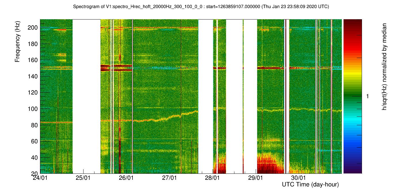
Figure 17: A typical 7-day spectrogram of the $h(t)$ channel, generated by the Spectro tool and allowing the monitoring of a wandering spectral line whose main frequency was first stable around 83 Hz before increasing up to around 100 Hz in about a day.

4.4.2 NoEMi and the (known) lines database

The noemi tool [77, 78] tracks on a daily basis spectral lines, both stationary and wandering ones, and searches for coincidences between the lines found in a main channel—typically the GW channel $h(t)$—and in a list of auxiliary channels. The noemi configuration defines several parameters and thresholds, like for instance: the threshold on the critical ratio for peak selection in the spectra, the frequency resolution (linked to the time length of the data segments over which the fft is computed), the name of the main channel, the list of auxiliary channels to search for coincidences. During O2, the noemi software produced daily results and looked for peaks in the spectra using a frequency resolution of 1 mHz. With this configuration noemi looked for coincident spectral peaks between the darm channel and approximately 40 auxiliary channels.

During the break between the O2 and O3 runs, the noemi software has been intensively modified, resolving the main issues identified in the old version. The original code was not well-structured (and hence difficult to modify) and also not fully-efficient CPU-wise. Furthermore, the original version produced several static files which were unessential for the final output. As a further improvement, the MySQL database which stores all parameters of each spectral line found during the run has been normalized, meaning that useless or redundant data have been removed and that the data storage is now more coherent. The database scalability has been improved as well, in order to allow storing more data and handling a higher load of requests. Additionally, a more dynamic interaction with the web interface used to browse the results has been introduced. The new version of the code has been used for the first time in O3.

During O3, noemi used the same set of ${\sim}$40 auxiliary channels as in O2, plus an additional set of ${\sim}$140 environmental channels, e.g. seismic, magnetic, and acoustic probes. The coincidence between a line in the GW strain signal and the signal of one of the environmental monitor, suggests that the noise line originates from a physical source such as a vacuum pump, a cooling fan, an electronic device, etc. This information helps to identify the instrumental origin of detected lines in the GW signal, and it has been included in the official Virgo-O3 line list publicly released by the gwosc [79]. Figure 18 illustrates the lines identified in the Virgo GW strain signal during O3.

Internally, lines that have been identified are stored in a dedicated database that includes detailed informations about them: most notably their times of appearance, and links pointing to the associated documentation (logbook entries, studies, mitigation actions, etc.). The contents of the database can be compared with a new noemi processing, to find out quickly which lines identified by noemi are already known and which ones are not.

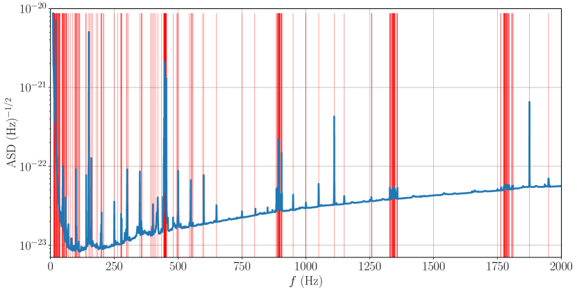
Figure 18: Virgo spectral lines identified during O3. The blue curve is the estimated asd of the Virgo strain signal during O3. Red vertical bars mark the frequency of the identified spectral lines. Lines parameters are listed in [79]. Most of the lines have been found by noemi.

4.4.3 Bruco

The bruco [80, 81] is a python-based tool designed to search for correlated noise by computing the magnitude-squared coherence between a main channel (typically, but not necessarily, the strain signal $h(t)$) and all other non-redundant auxiliary channels (about 3,000 channels in O3). Implementation details of the bruco software at EGO during O3 are described in A.3.

bruco main output is a table that contains, for each frequency bin, the ordered list of the auxiliary channels that are most coherent with the main channel. For each auxiliary channel in that list, the projected coherence (defined in A.3) is plotted and linked from the table. Assuming linear coupling, the projected coherence estimates the contribution of the noise witnessed by that auxiliary channel to the main one. Figure 19 shows bruco daily plots illustrating one example of noise contamination spotted during O3, which triggered a more in-depth investigation [31, 82].

bruco jobs were run regularly and automatically during the whole O3 run, with daily results displayed on a dedicated vim web page (see Section 4.1.3). In addition, bruco has often been used as an on-demand analysis tool to examine specific time periods.

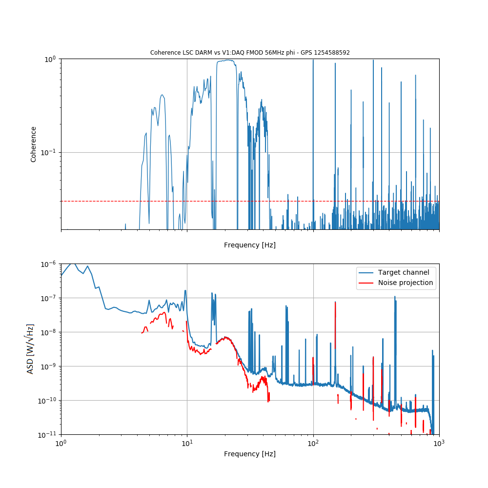
Figure 19: Selection of bruco vim daily plots evidencing noise contaminating the Virgo strain signal during O3. The top plot shows the coherence between the darm and the laser eom that produces the 56 MHz signals used for the arms length control. The bottom plot shows the asd of the darm signal (blue line) and the corresponding projected coherence (red line) in the frequency ranges where it was found significant enough. The noise was then found to originate from back-reflected light onto the laser bench, most likely due to a damage on the eom that component has been removed after O3.

4.4.4 MONET

The interferometer noise spectrum sometimes present some peculiar structures as a consequence of the non-linear couplings between different noise processes; these structures constitute two pairs of sidebands around known lines (see Sec. 2.3), which are not explained by means of the previously described linear coherence methods. One example of this kind of noise is bi-linear noise, generated by the coupling of two noise sources that jointly affect a third signal. In GW detectors, the main cause of this bi-linear noise is due to the upconversion of the low frequency seismic noise, that can affect the mirrors angular controls, which couples with some narrow-band noise processes, like power lines and calibration lines (see, e.g., [83, 59]).

The monet, [84], is a python-coded tool designed to investigate these sidebands. The main hypothesis at the basis of this tool is that the sidebands are due to some coupling of a carrier signal with the low-frequency (up to a few Hz) part of an auxiliary channel. Under this hypothesis, monet searches for coherence between a main channel (typically, but not necessarily, the detector strain signal) and a new signal, created as the product in the time domain of the chosen carrier signal and a modulator signal. The modulator signal is constructed by applying a low-pass filter to the signal of an auxiliary channel. More details are reported in A.4, including a typical monet output plot.

monet has been successfully used during the commissioning phase between O2 and O3 and during O3, allowing to spot the auxiliary channels contributing to the observed sidebands; for instance, it allowed to investigate the sidebands observed around the 1111 Hz line (injected for the purpose of the laser frequency stabilization control loop) [85] and the 50 Hz harmonics [86, 87, 88, 89].

4.5 Common LIGO-Virgo tools

4.5.1 DQSEGDB

For each data quality flag, the dqsegdb [90] stores the segments (integer GPS ranges) during which that particular flag is active, meaning that the set of conditions it is based on is fulfilled. For instance one such flag tags the GPS segments during which the Virgo detector is taking data in science mode, meaning that the data acquired live is expected to meet the quality criteria for physics analysis. There are two ways to fill this database with Virgo flags:

• online, during the data taking, through the SegOnline server that is compiling information provided by various data streams;

• offline, by completing or fixing existing segment sets, or adding new data quality flags to monitor additional conditions.

A versioning system is used to keep track of changes in segment lists that can modify a particular flag, i.e. that impact offline analyses, by changing the contents of the dataset they are processing. By convention, the highest version number corresponds to the best (most recent) segment list and is the one queried by default.

4.5.2 GraceDB

During O3, the gracedb [91] has been the central place where informations about transient gw candidates was uploaded and stored: online search triggers, source localisation estimates in the sky, data quality information, other metadata, etc. In particular, gracedb triggered automatically frameworks like the dqr through the lvalert [92] when candidate events of interest were identified; and, consequently, dqr results (see Section 6.1) got uploaded back to gracedb as soon as they became available. gracedb has a public-faced portal that provides information about the public alerts shared with the astronomer community, while most of its data are private and reserved to the LIGO, Virgo and KAGRA collaborations.

5 Real-time data quality

Online data quality was a key challenge to tackle for DetChar during the O3 run. The availability and the reliability of that information, supporting the data taking, had to be high in order to allow the real-time transient gw searches to make the best use of the Virgo data. Significant candidates identified by those analyses— usually found in data from at least two of the three detectors of the global network, but sometimes significant in a single instrument— would then lead to public alerts, used by telescopes to search for counterparts of potential gw signals.

In this section, we first describe the different blocks of the Virgo online data quality architecture, in use at EGO during the O3 run. This framework matches the dataflow shown in Figure 4 and is complemented by the vetting of the most significant triggers identified in low latency, described in the following Section 6. In summary, real-time information about the detector status was combined with fast data quality estimators to produce a single integer channel sampled at 1 Hz, the Virgo state vector. That state vector was shipped alongside the gw strain channel $h(t)$ to computing centers where data were analysed in real time. Its integer value was constructed by gathering several binary information (schematically: good vs. bad) encoded as bits; that bit pattern would later be decoded by the analysis frameworks to discard any bad data. Parallel to this data analysis stream, this information—the detector status plus the real-time assessment of the data quality—was automatically uploaded by a dedicated online process (called SegOnline) to dqsegdb.

Finally, we present the experience gained during O3 with additional data-quality inputs, called veto streams whose aim is to help searches to reduce their false alarm rate by identifying triggers that are very unlikely to be of astrophysical origin.

5.1 The Virgo O3 online data quality framework

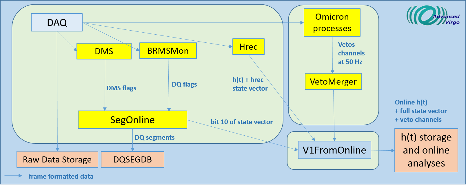
Figure 20: Online architecture to produce data quality products during the O3 run. The status of the interferometer is monitored by a dedicated Metatron server (see Section 3.2). Data quality flags are generated by dedicated servers: the dms, the BRMSMon process (environment), the VetoMerger process (large deviations in auxiliary signals), the Hrec process ($h(t)$ reconstruction), and the Omicron algorithm (glitches in $h(t)$ and auxiliary signals). Data quality segments are then generated by the SegOnline process and saved in the LIGO-Virgo segment database, while the online $h(t)$ stream, the state vector and the veto channels are sent to online data analysis pipelines through the V1FromOnline server. See text for additional informations.

The online data quality architecture is designed to deliver data quality products to online transient searches. It is based on a set of servers connected to the DAQ and providing relevant information about the quality of the data (raw data plus the reconstructed $h(t)$ stream). In the following, the main elements of this architecture, summarized in Figure 20, are presented.

5.1.1 State vector

Table 3 defines the 16 bits of the Virgo state vector integer channel in use during the O3 run. A bit is said to be active when its value is 1, meaning that the corresponding check is passed. A value at 0 means instead that a problem, or a non-nominal state, has been detected. The information provided by these bits is on purpose partially redundant, in the sense that several bits can be at 0 when proper data taking conditions are not met. During O3, the bits 0, 1 and 10 were required to be active to have the 1 s data frame processed by real-time analyses.

Table 3: Definition of the bits of the Virgo state vector during the O3 run (see text for details).

Bit number	Active when
0	$h(t)$ successfully computed.
1-2	Science mode enabled.
3	$h(t)$ successfully produced by the calibration pipeline.
4-7	Bits irrelevant for the present discussion:
	either redundant with other bits or unused during O3.
8	No DetChar-related hardware injection
	(see Section 7.2 for more details).
9	No continuous wave hardware injection
	(the only type of non calibration-related injections
	performed for a short period during O3, while taking nominal data).
10	Online data quality is good (no CAT1-type veto).
11	Virgo interferometer fully controlled,
	with a nominal working point or close to it.
12-15	Not used.

5.1.2 Online CAT1 vetoes

During the O3 run, the problems detected online and leading to CAT1 vetoes are listed below. These saturation checks were combined using a logical OR to produce CAT1 vetoes with a 1 s granularity. Section 7.4.1 describes the corresponding set of offline CAT1 vetoes, used by all analyses processing the final O3 Virgo dataset— and obviously including these online CAT1 vetoes.

• No saturation of any of the 4 dark fringe photodiodes, using the ‘DC’ (from 0 to a few Hz) and ‘Audio’ (from a few Hz to 10-50 kHz) demodulated signals.

• No saturation of the correction signal of any of the 16 suspension stages monitored.

• No saturation of the rate of glitches reported by the online Omicron framework for the darm correction channel.

5.1.3 SegOnline

Any channel provided by the daq or by the online processing (for instance dms monitors or BRMSMon process) can be used by the SegOnline process to build segments of data quality flags which are sent online to dqsegdb.

SegOnline writes down segments into XML files with a latency of about 10 s and those XML files are then read by a rsync process to upload the segments into dqsegdb every 5 min. Such data quality segments can be then used by any analysis or can be viewed and downloaded through a dedicated web interface [93].

5.2 Veto streams

Low-latency transient searches are limited by glitches in the $h(t)$ data. Each search pipeline is sensitive to specific families of glitches. The online data quality architecture is designed to deliver a channel to flag glitches relevant to a given low-latency pipeline. These channels are called veto streams. A veto stream is a time series which can only take two values: 0 means good quality and 1 means bad quality. A veto stream is generated by the VetoMerger process which combines information from many online data quality processes, which must be carefully selected to target the glitches limiting the search of interest.

Some Omicron processes (Section 4.3.1) are configured to select triggers detected in auxiliary channels with a signal-to-noise ratio above a threshold tuned with the upv algorithm (Section 4.3.2). These triggers are known to witness glitches in the $h(t)$ channel. When this is the case, the veto channel is set to 1. VetoMerger also ingests the data quality flags generated by BRMSMon (Section 4.2.2) to veto environmental disturbances.

In O3, the veto stream system was experimented as an input to one of the low-latency searches for compact binary mergers, PyCBC Live [94, 57]. The veto stream, named DQ_VETO_PYCBC, combined two elements: a veto channel delivered by Omicron to target scattered-light glitches, and a data quality flag produced by BRMSMon to tag occasional glitches associated to lightning strikes. A conservative approach was adopted to tune the vetoes: their thresholds were set at high values to reliably flag really limiting glitches, while keeping the rejected time low. As a result, only 0.05% of the O3 science time was flagged by the DQ_VETO_PYCBC veto stream. PyCBC Live used the veto stream to simply prevent the generation of a candidate event from Virgo data, or remove Virgo’s contribution from a LIGO-Virgo candidate, during periods of active veto. In future runs, the veto streams may be integrated in a more general framework based on auxiliary channels to discard or down-weight transient noise events.

The effect of the veto streams has also been evaluated on the PyCBC offline analysis, using Virgo single-detector triggers generated by the broad-space PyCBC search [95] during the period from April 1 to May 11, 2019. The triggers used for this study are ranked by the reweighted snr, the signal-to-noise ratio returned by the matched filtering technique, weighted by the result of $\chi^{2}$ tests that quantify how well the time-frequency distribution of power observed in the data is consistent with the one expected from the matching template. For practical reasons, only triggers with reweighted snr higher than 6 are considered. To evaluate the impact of the vetoes on the offline search, triggers with a merger time belonging to a vetoed segment are removed. The study is performed separately for vetoes targeting scattered-light glitches and glitches from lightning. The fraction of vetoed triggers is shown by the red points in Figure 21, and in both cases is found to be of the order of $10^{-4}$, mainly affecting low reweighted snr.

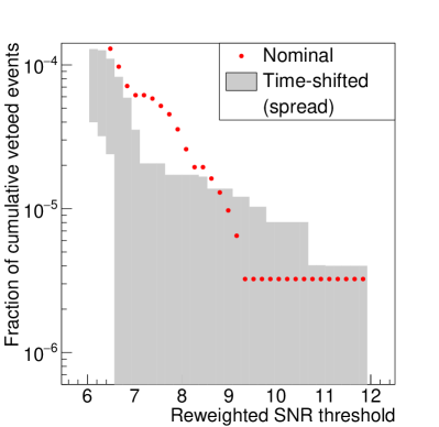
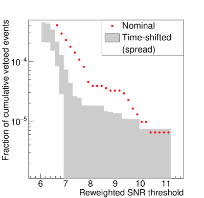
Figure 21: Cumulative fraction of vetoed PyCBC triggers with reweighted snr higher than a threshold, as a function of the threshold value. The grey band shows the envelope of the fraction of rejected triggers from 1,000 time-shifted trials (covering from the minimum to the maximum obtained value), while the red points show the results obtained using the unshifted veto segments. The fractions are relative to the overall number of triggers generated by the offline PyCBC broad-space search. The left plot considers vetoes targeting scattered-light glitches, and the right plot considers vetoes associated with glitches from lightning.

The statistical significance of the impact of the vetoes on the offline PyCBC triggers is assessed by performing a time-shifted analysis, and using it to calculate the probability that the fraction of vetoed triggers obtained from the unshifted analysis corresponds to triggers that have no correlation with the veto segments. To this end, we shift the veto segments by a constant time offset and recompute the fraction of vetoed triggers, obtaining a “null sample” that we can compare to the fraction obtained using the unshifted segments. Note that the null fraction is rescaled to account for the overlap between the science mode segments and the time-shifted veto segments. We construct 1000 such null samples by repeating the time-shifted analysis with time offsets covering the range $[-50000,+50000]$ s in steps of 100 s. The spread (range between minimum and maximum) of the obtained fractions of rejected triggers is shown in gray in Figure 21. At a reweighted-snr threshold of 6, the unshifted fraction is higher than any time-shifted fraction, for both scattered-light and lightning vetoes. We conclude that the probability for the observed effect of the vetoes on the PyCBC offline triggers to be a statistical fluctuation is less than $10^{-3}$. For higher reweighted-snr thresholds of 8.5 (10.5), this probability is $2\times 10^{-3}$ ($2\times 10^{-2}$) for vetoes targeting scattered-light glitches, and less than $10^{-3}$ ($6\times 10^{-3}$) for vetoes associated with lightning glitches. It does therefore appear that scattered light and lightning strikes are correlated with a small population of PyCBC triggers, and that the veto streams can in principle be used to remove or down-weight these triggers.

6 Public alerts

As demonstrated with the extraordinary GW170817 [5] event from the O2 run, public alerts sent by the LIGO-Virgo network are key deliverables targeting the astronomy community. Yet, how successful these are depends on the accuracy of the information provided and of the latency at which they are delivered. For O3, the main contribution of the DetChar group to this effort has been the design and the implementation of the dqr framework. A dqr is a set of data quality checks, automatically triggered by the finding of a new gw candidate. Its output allowed the rrt team to vet the associated data in a timely way. Moreover, its usage extended way beyond the data taking period, as it was the main tool used to assess the data quality of all gw candidates identified by analyses, in some cases with a latency longer than a year (compared to when the corresponding data were acquired).

The implementation and the performance of the Virgo O3 dqr are described below, before summarizing how Virgo contributed to the LIGO-Virgo public alerts during the O3 run.

6.1 Data Quality Reports

6.1.1 Introduction

The dqr is a framework developed by LIGO and Virgo for the O3 run, in order to quickly gather enough information to vet the significant triggers found by the online transient gw searches. The goal is to either confirm the associated public alert, or have it retracted at once. All 80 public alerts delivered during O3 [96] (of which 24 retracted) have used this input.

A dqr runs on a computing cluster where the $h(t)$ strain channel and the associated raw data auxiliary channels are available in low latency. Therefore, each collaboration (Virgo at EGO and LIGO for its two detectors) was responsible for the implementation, the operation, the monitoring and the upgrade of its own dqr framework. There was however an agreement on a common format for the check outputs, originally developed by LIGO [97].

The dqr framework is triggered by gracedb through the lvalert protocol. A JSON payload received from gracedb allows for the generation and the configuration of a new dqr. The checks are then processed and their results are uploaded back to gracedb, alongside all the records associated with that particular gw candidate. In order for the dqr to be triggered, a candidate event is required to have a false-alarm rate below 1/day. This is a conservative threshold, much higher than that required to release the candidate as a public alert, but still low enough to keep the computational cost of generating the dqr under control. Therefore, in average, only a handful of dqr were automatically processed on a daily basis during the ${\approx}330$ days of the O3 run: not a high CPU load overall, but still about 20 times more dqr than the number of public alerts that had to be vetted.

6.1.2 Virgo implementation and contents

Figure 22 summarizes the Virgo dqr architecture used during the O3 run. When a trigger with a low-enough false alarm rate is received, a new dqr is created and configured, using information from gracedb. Then, the data quality checks are run in parallel on the EGO HTCondor [98] farm. As soon as a given check is complete, its results are uploaded back to gracedb. In parallel, the dqr progress and results are immediately available for Virgo DetChar experts and on-duty people, through an EGO-internal web server. The dqr format [97], originally developed by LIGO, is lighter and more versatile than the gracedb user interface: it ensures a direct access to the Virgo dqr outputs. The dqr webpage URL is automatically sent to the relevant internal mailing list as soon as the newly-created dqr processing starts.

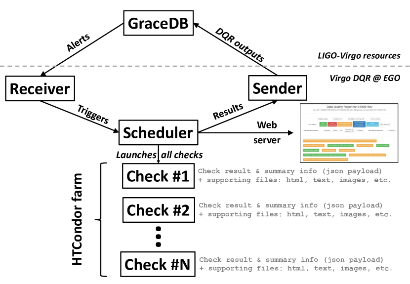
Figure 22: Schematics of the Virgo O3 dqr architecture. See text for a description of this workflow.

The Virgo dqr framework has evolved quite significantly over the course of O3. Partly to tune and improve the workflow based on the experience accumulated when stressing the system during an actual run, but mainly to extend the scope of the dqr by adding additional data quality checks. These new checks were either tests that had been foreseen but could not have been implemented by the start of O3, or new procedures that brought additional information that was found missing or useful when starting vetting real triggers.

Therefore, at the end of O3, the Virgo dqr included 34 checks, for a total of 99 jobs. There are roughly three jobs per check: the first, to run the code and process the data; the second, to post-process the check results and convert them to the LIGO-Virgo common dqr format; finally, the third to upload the results back to gracedb. Some checks included a fourth job as an initial configuration phase while others, developed specifically for the dqr, produced directly check outputs in the required dqr output format, meaning that those checks required one job less.

The Virgo dqr checks have been categorized in the following way.

• Key checks
  They bring information mandatory to properly vet a candidate event. This includes: the top-level status of the detector at the time of the trigger; some time-frequency spectrograms of the gw strain data at different timescales around that time; finally, the scan of the main data quality flags available online, in order to look for any obvious problem in the data.

• Characterization of the Virgo detector noise around the time of the trigger
  The noise transients (glitches) are inventoried and their potential overlap with the time-frequency extent expected for the candidate is probed— if applicable. In addition, searches for noise correlations in the time domain and noise coherences in the frequency domain are run, such as tests of noise Gaussianity and stationarity.

• Detailed Virgo status
  Several different analysis contribute to this global picture of the instrument. All data quality flags available are checked. In addition, the dms database is scanned to extract the snapshots closest in time to the trigger, to see what warnings or alarms were on— if any. Also, the logfiles of all the online servers running in the daq are scanned to spot errors that could be coincident with the trigger or impact it. Finally, various live data/reference comparison plots are generated to check the time series and distributions of a subset of the DAQ channels..

• Digest of the environment status
  This includes checking the seismic noise at EGO in various frequency bands corresponding to different sources (microseim related to sea activity on the Tuscany shoreline or local anthropogenic activities: see [30] for details), the sea activity and the weather.

6.1.3 Performance of the Virgo O3 dqr framework

This section briefly summarizes the performance of the Virgo dqr, via a statistical analysis using data from O3b that correspond to the final, most complete, version of that framework during the O3 run. As time distributions can include outliers due to occasional technical problems impacting the dqr dataflow somewhere along its way, from gracedb to the EGO HTCondor farm and back, the results presented in the following two tables include the $50^{\rm th}$ and $95^{\rm th}$ percentiles in addition to the mean values.

Table 4 provides the measured latencies for the processing steps that occur upstream of the dqr. The meaning of each row is reported below.

• The first figure is the difference between the time when the trigger is recorded in gracedb and the time when the corresponding data were acquired.

• The second measures the time needed for gracedb to send the lvalert and to have this message trigger the Virgo dqr framework upon reception.

• The third number reports the time needed to create and configure a new dqr instance, until it is ready for processing. One should note that this duration includes a 300 s wait time, imposed in order to allow gracedb to receive, process and gather all triggers found by the different online searches that analyse strain data in parallel and independently. The assumption is that, after these five minutes, the low-latency information available in gracedb should be optimal and stable in the vast majority of cases. Therefore, the actual dqr configuration phase only takes a few tens of seconds: the needed data are located in the low-latency streams just made available by the daq and the 30+ check scripts are generated one after the other.

• Finally, the last reported duration accounts for the time needed to start processing the dqr on the EGO HTCondor farm. This depends on the occupancy of the farm and of the EGO internal network performance.

Table 4: Summary of the performance of the low-latency + Virgo dqr dataflow during O3b, from the GPS time of a trigger to the start of the Virgo dqr on the EGO HTCondor farm: see text for details.

Operation	Time taken [s]
	Median	Mean	$95^{\rm th}$ percentile
Data acquired $\to$ Candidate on gracedb	52	166	331
Candidate on gracedb $\to$ lvalert trigger	4	4	11
lvalert trigger $\to$ Virgo dqr configured	331	339	383
Virgo dqr configured $\to$ Virgo dqr started	8	10	21

We can see that the mean time elapsed between the recording of the data by the different detectors and the creation of a new record in gracedb is under three minutes; the median time is even under one minute while the tail of the time distribution extends beyond five minutes. This includes the reconstruction of the gw strain channels; the transfer of these data alongside the associated online data quality information to computing centers; the processing of these data by real-time gw searches; the automated analysis of the results and the final transfer of trigger information to gracedb. Then, the new alert is received at EGO a few seconds later, triggering the creation and the configuration of a new dqr instance. Removing the compulsory wait time of 300 s, the dqr configuration takes a few tens of seconds only. Finally, about 10 additional seconds are needed on average to have the first dqr jobs processed on the EGO HTCondor farm.

Table 5 summarizes the performance of the Virgo O3 dqr framework in terms of running time. Each row corresponds to a category of checks. The quoted durations increase from one row to the next as each new set of checks includes the previous ones.

• The quick checks whose outputs are mandatory to vet a trigger take about 6 minutes to be all available, with a few minutes spread.

• Adding information about the Omicron triggers around the candidate takes about 10 more minutes. During O3, this latency was dominated by the fact that Omicron triggers were computed in real time and stored internally by the online server: they were only written to disk every 600 s, in order to allow the framework to cope with the incoming data flow. Work will be done prior to O4 to optimize this latency and to make the dqr aware of when the needed data have been written to disk, so that their processing can start immediately after.

• Omicron-scanning all the available channels (more than 2,000 in total, with the vast majority of them sampled at 10 kHz) around the trigger time requires 15-20 additional minutes.

• Finally, the full dqr took from 1.5 to 2 h to complete. The longest checks were bruco and upv, plus the scan of all online logfiles described above.

Table 5: Summary performance of the Virgo dqr processing during the last $\sim$100 days of the O3b run. The quoted durations include the time to upload dqr check results back to gracedb that usually takes from $\sim$5 to $\sim$20 s.

Operation	Time from start [s]
	Median	Mean	$95^{th}$ percentile
Quick key checks	374	383	619
Adding Omicron trigger distributions	868	816	935
Adding full Omicron scans	1740	2159	4690
End	5185	4954	6330

Another key figure of merit of the dqr framework is the number of (software) check failures per dqr instance. Table 6 shows the results of a statistical analysis based on the subset of the dqr that were automatically processed in real time during O3b because the candidate false-alarm rate was below the 1/day threshold. Only 13% (2%) of the dqr had 1 (2) failed checks. No exhaustive analysis of these failures has been performed, as most of these dqr were never checked by hand because the associated trigger was not significant enough. The two main causes of problems were, however, incomplete handling of edge-cases with the input data and actual bugs in processing algorithms. These issues did not affect the rapid vetting of any public alert during O3, and this framework worked smoothly as well for the validation of the offline events found later by the archival gw searches. Both issues are being addressed as part of the upgrade of the dqr framework for the O4 run.

Table 6: Percentages of the O3b Virgo dqr with 0, 1 and 2 unsuccessful checks respectively.

Number of unsuccessful checks	0	1	2
Percentage of O3b automatically processed dqr	85%	13%	2%

6.2 O3 public alerts

6.2.1 Public alerts retracted because of an issue with Virgo data

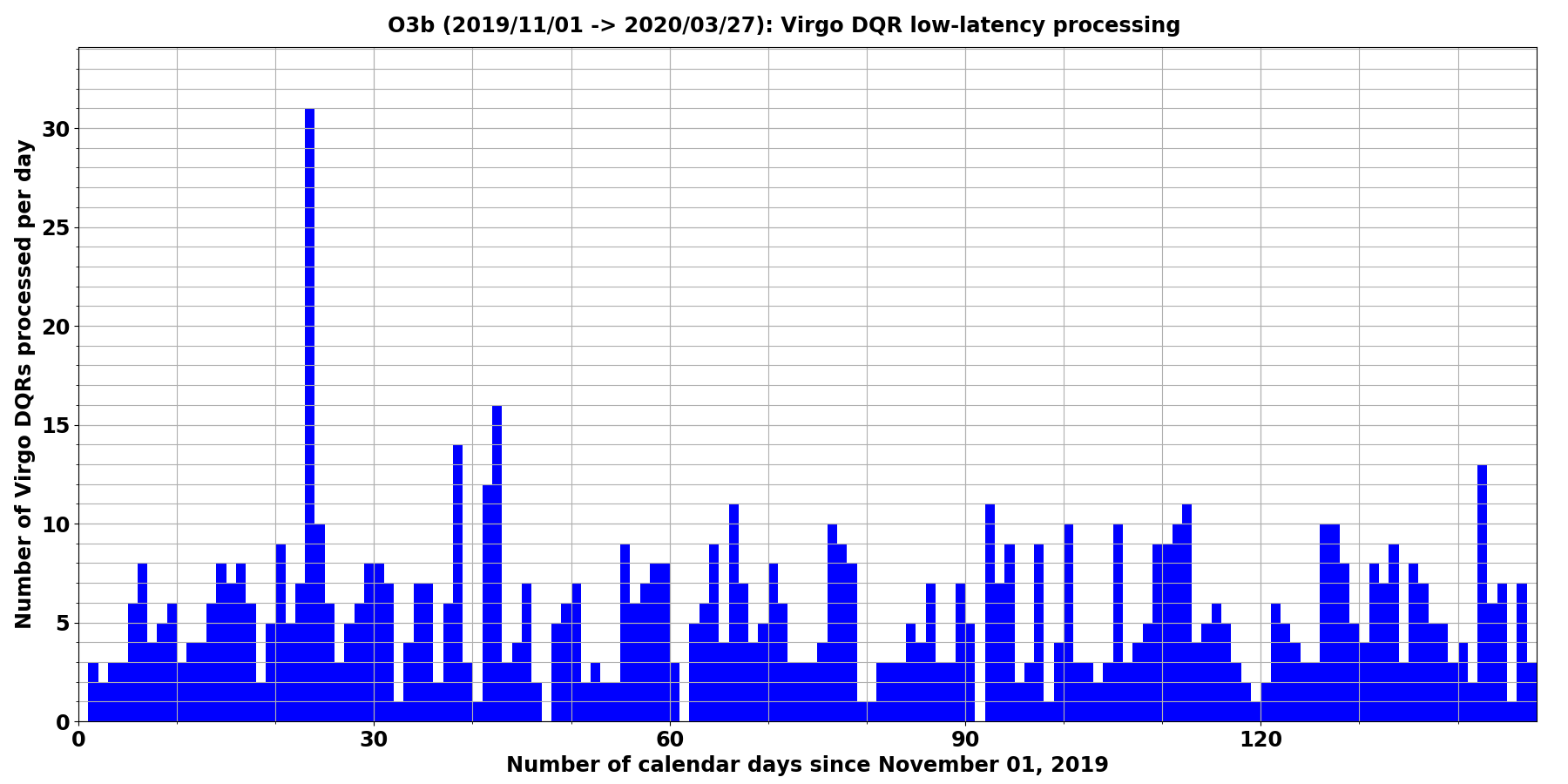
Figure 23: Number of Virgo dqr automatically processed per day during the O3b run. The peak of 31 entries corresponds to November 24, 2019 when there was a transient problem with the Virgo $h(t)$ reconstruction: that generated several online triggers, finally including S191124be that passed the public alert threshold and was promptly retracted.

During O3, 24 public alerts out of 80 have been retracted: 8 during O3a and 16 during O3b. Out of these retractions, only two were due to Virgo data:

• S191124be [99] was due to a problem in the noise removal procedure included in the reconstruction of the $h(t)$ GW stream [39]. Two such cleaning algorithms running in sequence started interfering, leading to a noise increase over time. An online pipeline started triggering on that excess noise, creating several non-astrophysical gw candidates in rapid succession (Figure 23) until one of them had a false alarm rate lower than the public alert threshold. That led to the generation of an automated alert that was then quickly retracted.
  A similar problem should not happen again in future runs for three reasons: i) improved noise cleaning procedures are being developed within the Virgo $h(t)$ reconstruction; ii) an online monitoring dedicated to such noise removal interferences will be in place during O4; iii) a monitoring of the pipeline trigger rates in gracedb will be running as well during future data taking periods, in order to spot quickly any misbehavior, like an excess trigger rate (thee case of S191124be) or the opposite: a too long data-taking time period without any trigger, even of low significance.

• S200303ba [100] was a single-pipeline trigger with most of its snr concentrated in Virgo. At that time, Virgo data were quite noisy due to bad weather. An Omicron-scan around the trigger time (Figure 24) showed evidence of scattering light noise at low frequency. The unusually-long delay to send out the retraction circular (about 80 min) was partly due to an issue with the Gamma-ray Coordinates Network broker connection.

  

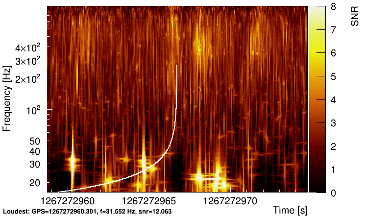
  Figure 24: Omicron spectrogram around the time of the S200303ba trigger. The search template time-frequency track (solid line) overlaps with low-frequency scattering-light glitches (yellow color) caused by bad weather.

6.2.2 Virgo contribution to O3 public alerts

Out of the 56 non-retracted O3 public alerts, 42 involved the Virgo detector. For 10 out of the 14 LIGO-only alerts, Virgo was not controlled in its nominal configuration at the GPS time of the trigger. This fraction is consistent with the average duty cycle of Virgo during O3 (see Section 3.5). For the four remaining alerts, described in detail next, Virgo was fully controlled at the time of the trigger and had a bns range consistent with its typical performance at that moment.

S190720a occurred during a $\sim 1$ min segment between lock acquisition and beginning of nominal observing mode, so Virgo data were not used for low-latency analyses. Offline analyses later confirmed S190720a as a significant detection and were able to use the low-noise Virgo data, finding a non-negligible amount of signal power in them. S190720a was published as GW190720_000836 in GWTC-2 [8].

S190910d occurred during nominal observing mode in Virgo. It was a marginal candidate, only reported by a subset of the low-latency searches. These searches did not find a significant amount of signal power in Virgo data, and did not report Virgo as being used for the candidate. S190910d was not confirmed by offline analyses.

S190923y occurred while Virgo was undergoing commissioning activity. It was not confirmed by offline analyses.

S200225q occurred while Virgo was undergoing a calibration run. Offline analyses confirmed S200225q as a significant detection and were able to include the low-noise Virgo data, although no significant signal power was found there. S200225q was published as GW200225_060421 in GWTC-3 [10].

7 Global data quality studies

This final section presents examples of global data quality studies made during or after the O3 run: noise transients, spectral analyses, classification of auxiliary channels based on their potential sensitivity to gw signals and offline data quality studies leading to the final Virgo O3 dataset.

7.1 Glitches and pipeline triggers

7.1.1 Glitch rates during the O3 run

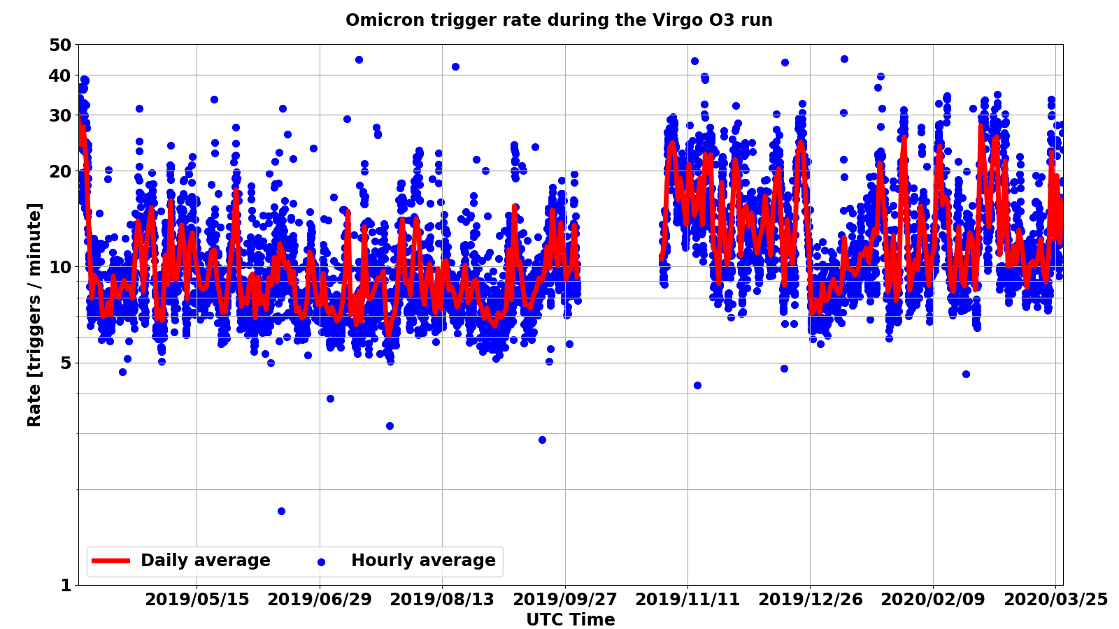
Figure 25: Virgo glitch rate, using Omicron triggers, for the final O3 dataset (Science segments that have not been CAT1-vetoed). The blue dots are averages over one hour while the red curve shows the corresponding weekly moving average. The gap in between O3a and O3b corresponds to the 1-month commissioning break.

During data taking, Omicron runs online on a few hundred channels, including the gw strain $h(t)$, and monitors glitches in real time: these triggers are stored on disk with a few minutes latency. Figure 25 displays the evolution of the glitch rate during the O3 run. Figure 26 provides more details by breaking the global Omicron glitch rate into snr (top plot) and peak frequencies (bottom plot). In these plots, the glitch rates have been smoothed by computing their weekly moving average to ease the reading.

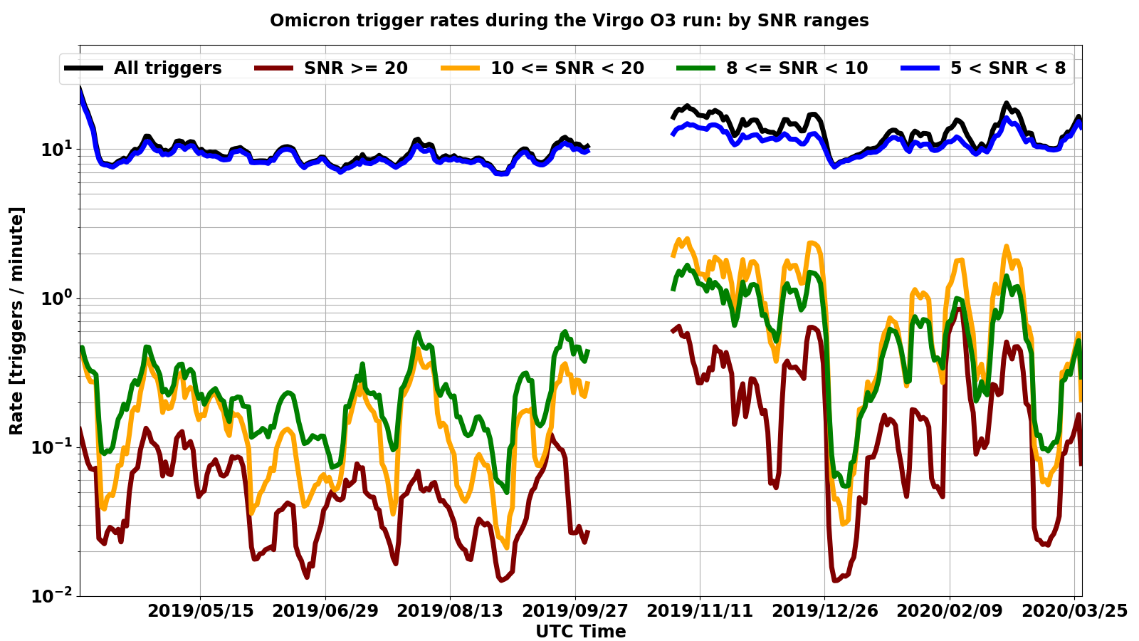
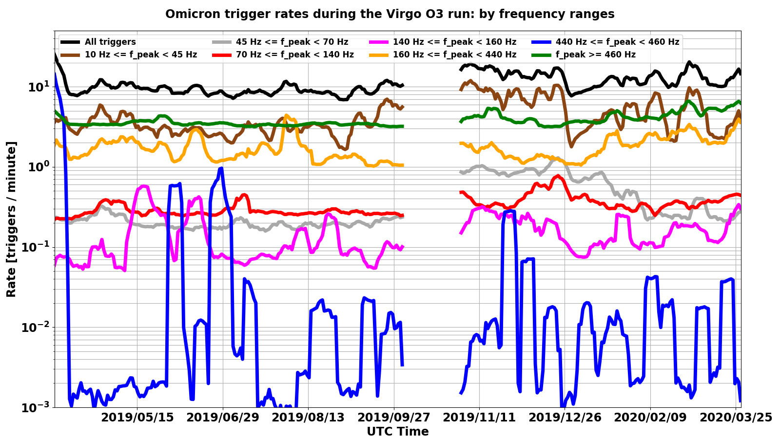
Figure 26: Glitch rates (weekly moving average) using Omicron triggers during the O3 run for Virgo— the gap in between O3a and O3b corresponds to the 1-month commissioning break. The top plot breaks the glitch rate into snr ranges, while the bottom one categorizes it in terms of frequency ranges for the glitch peak frequency. The choice of the frequency bands has been mainly driven by the need to isolate some frequencies: 50 Hz (mains fundamental power in Europe), 150 Hz (second harmonics of the mains) and the range around 450 Hz (another harmonics of the mains, plus the range in which the frequencies of the suspension wire violin modes are located).

The large majority of glitches identified by Omicron have a moderate snr: between 5 (the minimum value from which the Omicron trigger is kept) and 8. The highest trigger rate at the very beginning of O3a corresponding to glitches with a peak frequency between 440 and 460 Hz is an artefact due to a mis-configuration of the Omicron online server that was quickly fixed. The significant increase of the trigger rate in O3b with respect to O3a is mainly due to the bad weather conditions during the fall and winter seasons (see [30] for more details). The weather was actually very quiet in January 2020 and the associated drop in glitch rate is quite strong.

7.1.2 Offline searches

Non-stationary instrumental noise can potentially impact searches for transient gw, which must include methods to robustly separate astrophysical candidates from noise fluctuations. Despite the power of such methods, inspecting the candidates produced by a search remains a sensitive way to identify problematic operating conditions of gw detectors.

In this section, we focus on candidates produced from Virgo O3 archival data by one of the pipelines used by the LIGO and Virgo collaborations to detect compact binary mergers, namely PyCBC [95]. This analysis performs a broad-space search for compact binary mergers involving neutron stars, black holes, or a mix of both. It uses a bank of model waveforms and matched filtering to generate candidates from LIGO and Virgo data. Each single-detector candidate is ranked by a combination of its matched-filter snr and various statistics designed to reject candidates produced by non-stationary noise.

Figure 27 shows the rate of candidate events recorded by PyCBC from Virgo data. The horizontal axis shows either the matched-filter snr of the candidate (left plot) or a ranking statistic which combines the snr of the candidate and two $\chi^{2}$ signal-based discriminators [101, 102] (right plot). The vertical axis shows the rate of candidates that are ranked higher than the value in the horizontal axis .

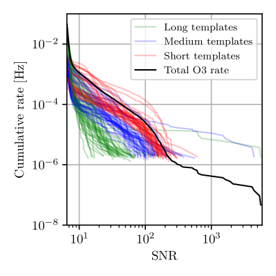
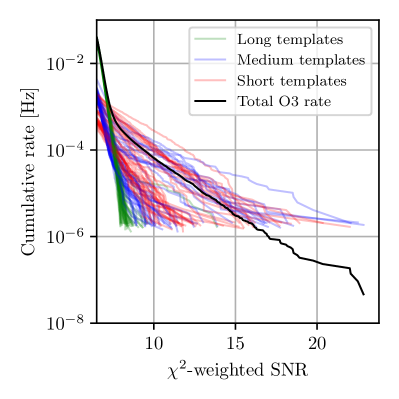
Figure 27: Rate of compact binary merger candidates produced from Virgo O3 data using a broad-space search based on PyCBC. Left: rate as a function of the matched-filter snr. Right: rate as a function of the reweighted snr, which combines the snr and two $\chi^{2}$ discriminators. Red, blue and green curves correspond respectively to templates lasting less than $0.6$ s, $0.6$–$4$ s, and more than $4$ s. Curves of the same color represent different chunks of Virgo data, each lasting $\sim 5$ days. The black curves show the rate over the entire run and search space. They extend to lower rates than the individual chunks due to the much longer duration of the entire run.

If the Virgo noise had been Gaussian and stationary throughout O3, we would expect the rate to decrease exponentially for larger and larger values of the ranking, and be independent on the template parameters and particular chunks of data. Instead, the rate-vs-snr curves show a more complicated behavior, with a large variation across the search space and particular data chunks. We observe a non-negligible rate at snr as high as 100, while astrophysical signals are typically expected to have snr between ${\sim}$5 and ${\sim}$10. After the application of the $\chi^{2}$ discriminators, the behavior changes drastically, and the exponential behavior of the rate is recovered, at least as long as we restrict to a subset of the search space. We still observe a large variation of the exponential slope and amplitude across the search space and data chunks, except for the longest templates (green curves of Figure 27), which are more robust to instrumental artifacts due to their particular time-frequency signature. However, the same variation is also seen with candidates from the LIGO detectors, and it is taken into account by the analysis when ranking the multidetector candidates [103].

A detailed inspection of the candidates in the tails of these plots shows that the highest snr can be attributed to a single segment of ${\sim}$15 min of data on November 11, 2019. These data contain narrowband, loud and rapidly-varying excesses of power (coming from transient problems with the noise subtraction algorithms used to reconstruct the gw strain channel $h(t)$) which temporarily affected the data conditioning algorithm used by PyCBC. Most of these high-snr triggers were removed by the $\chi^{2}$ discriminators, effectively vetoing the entire problematic segment. On the other hand, most top candidates by $\chi^{2}$-weighted snr are clearly associated with scattered-light glitches. We conclude that the $\chi^{2}$ discriminators used by PyCBC, which were designed for and tuned on LIGO data, are also reasonably effective in Virgo, and should be further developed to more effectively reduce the impact of scattered light.

7.2 Channel safety: channel (in)sensitivity to gravitational waves

Many Virgo data quality analyses aim at ensuring that gw candidates are of astrophysical origin and not caused by terrestrial noise. Typically, searches for correlations between auxiliary channels (monitoring the environment, the detector status, the accuracy of its control, etc.) and the $h(t)$ strain channel are run to produce vetoes, that reject times when such correlations are identified. This strategy can lead to a loss of interesting signals if any of the auxiliary channels is sensitive to gw, which means that it picks up disturbances induced in the detector by these. Hence, a good knowledge of the couplings of auxiliary channels to $h(t)$ is essential. To gather such information, a statistical analysis of all auxiliary channels is performed, using the approach proposed in [104].

This method relies on hardware injections that mimick the effects of gw on the detector, by moving in a deterministic way one of its test masses. They are used to workaround the fact that the transfer functions between $h(t)$ and most auxiliary channels are not well-known, nor understood. The injected signals are 0.6 s long sinusoidal Gaussian functions of various frequencies (between 19 Hz and 811 Hz) and amplitudes (SNR between ${\sim}$20 and ${\sim}$500). The frequencies injected are chosen to scan the entire detection band while avoiding any known resonant frequency (like violin modes). Each waveform is injected three times, spaced by 15 s.

This safety analysis assumes that glitches in a given auxiliary channel are distributed according to a stationary Poisson process, whose rate and $p$-value time series are measured using stretches of data during which no hardware injection is performed. These $p$-value time series are used to define a classification threshold. Then, a null test is applied to see whether the $p$-value distribution changes significantly in the presence of hardware injections. Auxiliary channels that exhibit anomalously small $p$-values (i.e. lower than the defined threshold) are classified as unsafe, meaning that they are likely to mirror excess power coming from the strain channel. The other channels, called safe are the only ones used to produce vetoes.

Virgo DetChar hardware injections were organized at short notice, in the few days between the anticipated end of the O3b run (because of the pandemic) and the moment when the detector was switched off. Among the ${\sim}$2500 auxiliary channels analysed, 69 are found to be unsafe. The safety analysis of these data allowed to validate the existing sets of safe and unsafe channels determined by a previous study. These results matched as well the a priori safe status one could infer based on the definition of the auxiliary channels, i.e. which measurements they perform and how they do them.

7.3 Spectral noise

The term spectral noise, introduced in Section 2.3, identifies the class of detector disturbances appearing as an persistent excess in the noise power spectrum estimation of the data.

Spectral noise has a negative impact especially on searches for persistent gw, which aim at detecting astrophysical or cosmological signals mainly through the identification of their spectral features. Two typical signal categories of persistent waves are cw [105] and a sgwb [106]. The signals are very weak with respect to the already detected coalescing binary emission. Due to their persistent nature, they can be looked for in the frequency domain where the accumulated power over long observation times can show up at a detectable level, after applying effective signal processing techniques. Moreover, some spectral features of the signals can help in discriminating them from detector noise. On the other hand, spectral noise can mask signals, or produce false candidates, in both cases reducing the search sensitivity.

Searches for persistent signals are typically run off-line, once long stretches of data have been collected. An early identification of spectral disturbances and of their instrumental source would allow to remove, or at least reduce, the source of noise, thus improving the quality of the data.

Different actions can be accomplished at the detector characterization level in support of data analysis. A first action is to identify, and possibly remove, the instrumental source of spectral noises as soon as possible during a data taking period. This is a non trivial task that typically requires a significant amount of work to nail down which detector component is responsible for a given disturbance and to eliminate the noise source, which may imply to replace the noisy component (for instance a cooling fan, an electric motor, etc.) [31], to shut it down (if not needed) or to modify it properly. This could consist, for instance, in shifting the frequency of a calibration line which non-linearly couples to another noise source, in order to move the noise line frequency into a less relevant band for the GW search [12, 107].

A second action is the use of additional techniques to differentiate between possible signals and other spectral features. These methods strongly depend on the analysis and on the type of gw signals searched An example of such techniques relies on the Doppler effect. An astrophysical cw signal is expected to be modulated in frequency by the Doppler effect, due to the Earth rotation, which induces a shift $\Delta f(t)\simeq f_{0}\frac{\vec{v}(t)\cdot\hat{n}}{c}$, where $f_{0}$ is the source frequency, $\vec{v}$ the detector velocity, $\hat{n}$ the unit vector identifying the sky direction and $c$ the speed of light. cw searches correct this Doppler effect, thus any monochromatic line present in the h(t) signal is spread by a maximum amount of $\Delta f_{max}\simeq 10^{-4}f_{0}\cdot cos{\beta}$— where $\beta$ is the ecliptic declination. This shift corresponds to up of hundreds or even thousands of frequency bins for typical cw searches.

Potential candidates found in the analysis lead to follow-up investigations to identify a possible instrumental source. This follow-up is also based on a combination of DetChar activity, to spot the source of the disturbances, and application of CW or SGWB algorithms to build confidence in the astrophysical nature of the candidate, see e.g. [108].

Although spectral noises cannot always be removed, it is still useful to characterize them by constructing a list of noisy lines. This list can be used to exclude those disturbing frequency bands from the analysis, or to veto candidates with frequency too close to those of these noisy lines

The identification of lines is typically done by automated pipelines (see Sections. 4.4.1, 4.4.2 and 4.4.3), based on

1. user-defined thresholds set on data power spectrum or on line persistency, defined as the fraction of fft, compared to the total number covering the full observation time, in which the “normalized” power content of a given frequency bin was above such a threshold (typically set to six times the average value);

2. by highlighting coincidences or significant coherence among different channels;

3. by highlighting a pattern in time-frequency maps of the data.

Candidates found in gw searches are subject to verification steps, in which the identification of possible noise counterparts is done by processing the data in the relevant frequency band and period of time and/or running manually one or more of the previously mentioned line identification pipelines, described in Sections. 4.4.1, 4.4.2, 4.4.3. In the following we report and discuss a few examples of lines identified in Virgo O3 data. Readers can refer to the LIGO-Virgo gwosc [79] for the full official list of lines.

7.3.1 Combs

Combs are families of lines separated by a constant frequency interval. Typically, noise combs are electromagnetic disturbances generated by digital devices (e.g. microprocessors, programmable communication devices like logical controllers, ethernet cables, wireless repeaters) that leak into the strain signal. Comb lines can have an impact on searches for persistent gw due to their large number and usually high strength. This makes the identification of combs an important task. There are several combs present in Virgo O3 data, which we describe in the following.

A 1 Hz spaced comb with 0 Hz offset was already present during previous runs. A new 1 Hz comb discovered during O3 has a 0.333 Hz offset with respect to integer frequencies. This comb was discovered following investigations of a line at 22.333 Hz that falls within a region of interest for the Vela pulsar cw search. The instrumental origin of the comb has been confirmed by finding lines at the same frequency in the magnetometers deployed at EGO.

Figure 28 shows the line persistency computed over the frequency range 21.8-23.5 Hz on O3 Virgo data. Both 1 Hz combs are clearly visible. Furthermore, there is a comb with 0.2 Hz spacing, whose origin is unknown. The grey area indicates the frequency region explored by a narrow-band cw search targeting the Vela pulsar. The strong line at 22.333 Hz produced an outlier in the search, which was discarded after its instrumental origin was identified.

Finally, two more combs which have been identified by DetChar studies, have both $\sim$9.99 Hz spacing, one with 0 Hz offset and the other with 0.5 Hz offset.

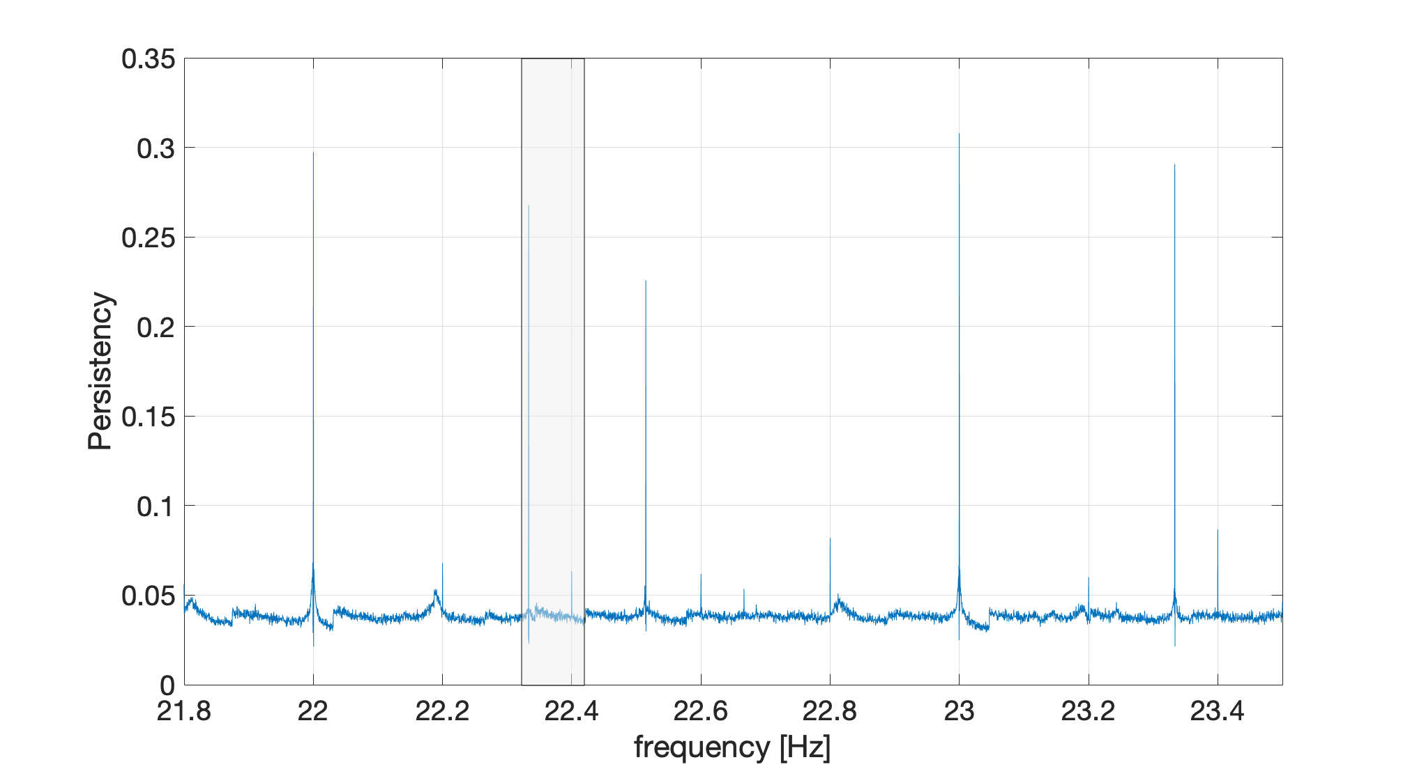
Figure 28: Plot of line persistency over the frequency band 20-30 Hz. The grey box identifies the frequency range covered by a narrow-band search of cw signals from the Vela pulsar in O3a data. The line at 23.333 Hz, which contributed to produce a candidate in the search is clearly visible. In fact, several other lines belonging to the 1 Hz comb, both at integer frequencies and shifted by 0.333 Hz, and to a weaker 0.2 Hz comb, are present.

7.3.2 Wandering line around 83 Hz – 84 Hz

A wandering line is a peculiar kind of spectral noise where the frequency of a spectral line changes with time, with no apparent reason. This is also called a drifting line once the mechanism driving the frequency change is at least partially identified, making its variations not entirely random anymore.

An example that triggered lots of DetChar investigations during O3 is the line, normally located between 83 and 84 Hz, as shown in Figure 17, that reached about 110 Hz at the maximum of its excursion and had variations of a few Hertz over about one hour [109, 110]. Its origin dates back to the Virgo commissioning run 10 (C10) of August 2018 [59], and possibly even earlier, in the preparatory phase preceding O2 [111]. Neither of the mechanism that make the line to depart from its typical frequency of about 83 Hz or what produces its variations with time have ever been understood, although several data analysis techniques have been applied and newer ones developed for line tracking [59]. An analysis with Bruco (see 4.4.3) revealed no witness channel coherent with $h(t)$ around that line. Moreover, we tracked the frequency evolution of this line, and we correlated the corresponding time series with the auxiliary channels monitoring Virgo [109]. This technique has proven successful in the past, in the case of drifting lines driven by the temperature of some optical components [112], but has produced no convincing correlation in the case of this line, whose origin has remained unknown.

7.3.3 Spectral noise bump around 55 Hz

Figure 29a) shows the power spectrum of the Virgo gw strain channel $h(t)$ computed at two different dates, February 26 and March 2, 2019 (before the start of the O3 run), showing that a wide bump around 55 Hz had been cured in the meantime. Indeed, a detailed study had shown that this disturbance was present most of the time and was observed also in the prcl channel. This allowed to remove most of this noise excess when producing the reconstructed strain $h(t)$, by accurately subtracting the remaining prcl contribution [39]. Note that this 55 Hz bump affected the frequencies around 55.6 Hz, where the cw signal possibly emitted by pulsar PSR J1913+1011 is expected. Furthermore, this bump was located within the most sensitive region of the Virgo spectrum for an (isotropic) stochastic background search.

7.3.4 Spectral noise around the 50 Hz power line frequency

The GW strain signal in the frequency region between 45 Hz and 55 Hz was significantly affected by ambient electromagnetic fields originating from the interferometer infrastructure. This noise was studied and mitigated in subsequent steps during the run [31].

The intense 50 Hz line, corresponding to the frequency of the electricity mains, was mitigated and substantially eliminated from $h(t)$ (see Figure 29b), by implementing a feed-forward noise cancellation scheme using as sensor a voltage monitor of the detector uninterruptible power supply system [31]. This operation did not reduce the 50 Hz harmonics also present in the $h(t)$ spectrum (see Figure 6) because they are not due to a non-linear response of the interferometer. They are present in the global environmental disturbances and enter the GW strain channel through different coupling paths.

Sidebands of the mains frequency, at approximately 49.5 Hz and 50.5 Hz, were generated by the pulse width modulation of the electric heater controller of the imc building. The noise was mitigated by decoupling the electric ground of the building from the central experimental area with an isolation transformer.

Figure 29c) illustrates a wide-band noise affecting the same region. The origin of this noise was eventually found to be a noisy static voltage accidentally applied to the signal wires of the motors used for positioning and balancing the WE mirror suspension, then coupling capacitively to the mirror coil actuator wires. The noise was mitigated by un-plugging the drivers of the motors, which are not used in science mode.

Finally, Figure 29d) illustrates a family of lines between 47 Hz and 49 Hz which have been identified as vertical mechanical modes of the last stage of the test mass suspension system. These modes are excited by ambient magnetic fields coupling to the magnetic actuators along the suspension chain. This noise was suppressed by an active mechanical damping of the modes.

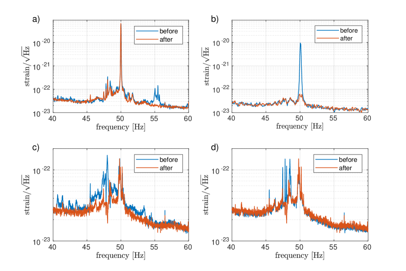
Figure 29: Four steps of the reduction process of the strain spectral noise between 40 Hz and 60 Hz during O3. In all sub-figures the blue curve is before the mitigation, and the red curve is after the mitigation. a) Cancellation of the spectral noise structure around 55 Hz which was common to the prcl signal. b) Subtraction of the 50 Hz line associated to the power grid. c) Mitigation of a wide-band noise associated to the motor driver crate of the WE suspension. d) Suppression of a few noise lines associated to mechanical modes of the test masses payload.

7.4 Offline data quality

7.4.1 Offline studies and checks

While Section 5.1.2 describes the online CAT1 vetoes, we focus here on the final set of offline CAT1 vetoes. They supersede online vetoes and have been used by all analyses processing the final O3 Virgo dataset. These include analyses using the O3 LIGO-Virgo public dataset: that is why the gwosc website [113] includes detailed public information about these vetoes [114].

Like the online CAT1 vetoes, all these veto flag segments of bad data that are unusable. They are defined with a 1 s granularity and the figure-of-merit used to quantify their impact is their dead time, that is the fraction of Science time that is removed by applying them individually. Yet, the vetoes are not independent and they may overlap. Therefore, they are meant to be applied globally on the dataset, by taking the logical OR of all of them.

The offline vetoes defined during the O3 run can be classified into three main categories.

• The duplication—after crosscheck and potential additions or fixes—of online CAT1 vetoes: this includes the saturations of dark fringe photodiodes or mirror suspensions, and the monitoring of the reconstructed gw strain $h(t)$.

• The upgrade of existing online vetoes: the excess rate of glitches is monitored offline using $h(t)$ whereas only the darm channel could be used online due to latency constraints.

• The addition of new vetoes, based on information that was not available in low latency, or that was not known at the time online flags were generated. These categories are described below.

  • Checks of the consistency and of the completeness of the files storing the $h(t)$ GW stream: these vetoes flag segments in which $h(t)$ is missing or contains missing samples.

  • The $h(t)$ stream is reconstructed by blocks of eight consecutive seconds of data. Therefore, a control loss can possibly impact up to the eight seconds of data that predate it. As the exact time of a control loss is not easy to define, the last ten seconds preceding each recorded control loss have been removed.

  • The Science dataset has been scanned accurately to identify segments during which the detector was not taking good quality data, contrary to what its status was indicating. These segments were removed from the final dataset.

  • Finally, a workaround was applied to the detector control system during some weeks in O3b in order to mitigate transient data losses due the failure of an hardware component. That patch allowed to maintain the working point of the instrument, thus sparing a ${\sim}$20 min control acquisition procedure each time it prevented a global control loss. Yet, the application of that workaround could degrade the quality of the data. Thus, the impacted segments were removed from the final dataset, with some safety margin on both ends (the last 10 seconds before having the control patch be applied automatically, and the first 110 seconds following the end of the transition back to the nominal control system).

Table 7 summarizes the impact of CAT1 vetoes on the final O3 Science dataset: overall, only 0.2% of the Science data have had to be removed due to various problems.

Table 7: Virgo O3 offline Science dataset and CAT1 vetoes.

	O3a	O3b	O3a + O3b
Science dataset	12,057,731 s	9,611,843 s	21,669,574 s
Logical OR	18,802 s	20,636 s	39,438 s
of all offline CAT1 vetoes	(0.16%)	(0.22%)	(0.18%)

Conversely, a few minutes of good quality data that had not been included in the online Science dataset for various and clearly understood reasons (software issue, human error, etc.) were added to the offline, final, dataset.

7.4.2 Event validation

To assess whether the detection alerts produced by transient searches [57, 94, 115, 116] should be considered as “candidate events”, a procedure of validation is implemented after each generated trigger [10, 45]. This task has the role to verify if data quality issues, such as instrumental artifacts, environmental disturbances, etc., can impact the analysis results and decrease the confidence of a detection, or even foster a rejection [117].

The validation of the online triggers found by gw transient searches includes two separate stages. A prompt evaluation is typically completed within few tens of minutes after an event trigger has been generated, as represented by the data flow in Figure 4. Its goal is to determine a preliminary detection confidence and sky localization, in order to deliver public alerts to the astronomy community and support for multi-messenger follow up observations [117], as described in Section 6, or to vet that trigger if evidence of severe contamination from non-astrophysical artifacts is present. A team of DetChar shifters is in charge of this task as part of the rapid-response team (Section 3.4). The decision about the event is primarily based on the quick results provided by the dqr within a few minutes from the trigger. This decision takes into account the evaluation of the operational status of the detector and its subsystems, the environmental conditions, as well as preliminary checks on the strain data. In particular, the shifters are asked to verify the presence of excess noise, namely glitches, around the time of the trigger and the validity of the hypotheses of stationarity and Gaussianity of the data, as discussed in Sections 4.2.3 and 4.3. Moreover, it is examined the possible presence of correlations between the strain data and the auxiliary sensors, which may advise a non-astrophysical origin of the trigger.

With higher latency, a second stage of validation is performed by a validation team to finally check candidate events before publications, including those found by offline analyses [56, 95]. Besides of (double-)checking the astrophysical origin of the event trigger, the main purpose of this process is to carefully assess whether the parameter estimation of the source properties can be affected by noise artifacts. This procedure takes advantage of dedicated reruns of the dqr, as well as from additional tools and metrics, including, for example, signal consistency checks [45, 118].

For those events where non-stationary noise, such as glitches, are found in the vicinity of the putative gw signal, or even overlapping with it, a procedure of noise mitigation is implemented [119, 120]. During O3b, such process has involved 12 events, including one with Virgo data, GW191105e [10, 121], where the process of mitigation and validation of the data quality has improved the parameter estimation results and credibility. Various O3a events have undertaken a preliminary version of this procedure [8].

8 Preparation of the O4 run

The LIGO-Virgo O3 run has lead to the discovery of dozens of new gw signals from compact binary mergers, which have boosted our knowledge of these populations in our local Universe and allowed further, more stringent, tests of general relativity. The O3 run has also been the first long data-taking period for the adv detector. Thus, it represents a full-scale, extended and non-stop stress test of the organization and work methods of the Virgo DetChar group. The experience accumulated during these 11 months will form the base of the DetChar activities, both to prepare and operate for O4 and the following runs.

Although the Virgo DetChar group has fulfilled all its main requirements during the O3 run, work has been going on since then to improve its performance and extend its activities. In particular, the anticipated differences between the O3 and O4 runs lead to new challenges that the group should tackle. The adv detector will have evolved significantly, with the completion of the Phase I of the adv+ project. The main changes on the instrument side are the addition of the signal-recycling mirror in between the beam splitter and the output port of the Virgo interferometer, a higher input laser power and the implementation of frequency-dependent squeezing. This new configuration will require dedicated instrument characterization activities, while many new data quality features will have to be discovered, understood and later mitigated or solved. On the data analysis side, progress in terms of sensitivity while keeping the network duty cycle high will lead to more gw detections. On the one hand, more work will be required to validate this excess of signal candidates compared to O3; on the other hand, the triggers passing a given false alarm rate threshold will remain dominated by noises, meaning that the bulk of computing resources used by the Virgo DetChar group will not change significantly.

Gathering experience from the past and predictions for the future, a few top priorities have emerged for the DetChar group. A first and obvious one is to broaden the scope of the DetChar monitoring, to make sure that no relevant area remains uncovered, from raw data to the final analyses. Then, the latency of the various DetChar products should be decreased when it is relevant and possible: either by making the corresponding software framework more efficient, or by processing new data more regularly. Finally, some emphasis should be put on increasing the automation of the DetChar analyses and the reporting of their results. In that respect, the dqr is a good example of the realization of these plans. Parallel to common LIGO-Virgo-KAGRA developments on the framework architecture to make dqr more uniform among the three collaborations and to improve its performance, additional data quality checks will be implemented. They will provide combined results that should give a partial digest of the global vetting of a given gw signal candidate.

The increase of the information available and the help to identify quickly its most relevant points should allow maintaining, if not improving, the high and steady level of Virgo performances observed during O3.

Appendix A Additional tool information

In this Appendix, we describe in more detail some of the data analysis techniques presented in Section 4, and their implementations into tools. A.1 and A.2 provide additional information on the statistics adopted to test the hypotheses of stationarity and Gaussianity with the bristol and rayleighSpectro tools, and their interplay. A.3 and A.4 are devoted to the tools for spectral noise investigations BruCo and MONET. The former uses the coherence as a figure of merit to study the linear transfer of power between a set of auxiliary channels and a main channel, usually the GW strain $h(t)$. The latter investigates non-linear couplings between channels, by studying the coherence of the main channel (usually $h(t)$) with a synthetic one, created by modulating a carrier signal (either an existing DAQ channel or a sinusoid with a fixed frequency) with the low-frequency part of an auxiliary channel.

A.1 BRiSTOL - a Band-limited RMS Stationarity Test Tool

This statistical test aims at verifying the hypothesis of wide (or weak) sense stationarity of the data, i.e. that the covariance function is left unchanged by shifts in time. We test this by verifying that subsequent psd estimates, in predefined frequency bands, are compatible with the same probability distribution. The corresponding test statistics are based on a set of brms time series, estimated on an equal number of bands:

$$\mathit{BRMS}_{t}(b)=\sqrt{\int_{f\in b}\hat{S}_{t}(f)\,df},\qquad\mathrm{for}\quad b\in\left\{[f_{1}^{\max},f_{1}^{\min}],\ldots,[f_{K}^{\max},f_{K}^{\min}]\right\}$$ (4)

for data $x_{t_{n}}$ recorded at Nyquist rate $f_{S}$, $t_{n}=t+n/f_{S}$, where $\hat{S}_{t}(f)$ is a psd estimate referred to time $t$, and obtained with the periodogram method [122]:

$$\hat{S}_{t}(f_{k})=\frac{1}{N}\bigg{|}\sum_{n=0}^{N-1}x_{t_{n}}e^{-2\pi i\,nf_{k}/f_{S}}\bigg{|}^{2},\qquad f_{k}=\frac{k\,f_{S}}{N},\quad\text{for}\quad k=0,\ldots,N-1$$ (5)

Two modifications have been implemented to make (4) more suitable for the study of transient noise, in particular to highlight slow non-stationarity. Firstly, spectral lines (refer to Section 4.4.2 for more details) have been removed from the integral. These are narrow features in the psd of the data, originating from resonances in various parts of the interferometer and their harmonics. Their intensities can be orders of magnitude larger than the neighboring noise floor. Hence, if a line is present in a band where we are about to compute the brms, it is likely to dominate the final estimate, and also the corresponding fluctuations, preventing us from probing the features of the underlying noise floor. To remove these lines, we identify them with an algorithm similar to the one developed for the noemi pipeline [77], and based on the prominence of their psd [123].

Second, glitches are also typically removed from the brms time series. These fast transients can manifest at a rate of about 10 per minute, as shown in Figure 25, which means that every data segment longer than a few seconds is likely to contain one of them. To focus on slower noise transients, which typically are not targeted by tools specifically devoted to excess power identification, such as those presented in Section 5, we must exclude the data segments affected by glitches from the stationarity test. This is done by means of an algorithm based on a rolling median absolute deviation, defined as the median absolute difference from the median, to identify outliers in the brms data.

Then, the time series corresponding to the resulting modified brms are divided into “chunks” where estimate their empirical distribution function. The stationarity hypothesis is tested by means of a two-sample Kolmogorov–Smirnov test [60] for each pair of consecutive chunks, whose $p$-values are compared to a test significance $\alpha$ (to be decided in advance), and the (null) hypothesis of stationarity rejected when the latter is exceeded.

There are two advantages in using the brms. First, averaging over the frequencies of each band has a similar variance reduction effect than the means in Welch’s psd estimation method [124]. This in turn allows a finer time resolution while maintaining a moderate variance for our test statistics, that is, the empirical distribution of the brms. Second, the various non-stationarities typically manifest in specific frequency bands, closely related to the noise source that generated them. For example, the main harmonic of scattered light is usually visible below 30 Hz; non-linear and non-stationary couplings of the angular controls with the 150 Hz harmonic line are characteristic of a tight region around it, etc. So, without losing much of resolution, we can perform the noise characterization directly on these bands instead of on each frequency bin comprising the spectrum of the signal.

A.2 rayleighSpectro - Gaussianity test

Similarly to what was discussed for the stationarity hypothesis, Gaussianity is likewise important to be tested separately in the different regions of the spectrum where noise sources can show up. rayleighSpectro does this by means of a consistency check on the psd estimated from the data with what is expected for stationary Gaussian noise. Indeed, if the data is compatible with the hypothesis od Gaussianity, the periodogram estimator in Equation (5) is asymptotically (with $N$) described by an exponential distribution of parameter $S(f_{k})^{-1}$ [125], where $S(f_{k})$ is the process psd. The corresponding asd estimator, obtained as the square root of Equation (5), is described by a Rayleigh distribution with parameter $\sqrt{S(f_{k})/2}$. The scaling property of this distribution can be used to construct consistency tests. For example, the standard deviation of the asd estimates obtained on non-overlapping segments provides an estimator of the standard deviation of this variable, which equals $\sqrt{(4-\pi)\,S(f_{k})}/2$. Similarly, the mean of these estimates provides an estimator of the mean: $\sqrt{\pi S(f_{k})}/2$. The ratio of these two quantities gives a statistic that, at each frequency $f_{k}$, is asymptotically equal to a constant whose numerical value is given in Equation (1), in the null hypothesis that the data is described by a stationary and Gaussian distribution. The actual value of the previous quantity for a finite number of averages and the corresponding critical values for performing statistical tests have been computed in [126, 61].

By dividing the data into chunks of duration $\Delta t$, one can obtain a time–frequency map, similar to a spectrogram, showing with time resolution $\Delta t$ the frequencies and times where the data significantly depart from the expected value of Equation (1). Smaller values of this statistic are associated with data having smaller fluctuations than those expected for a Gaussian process; spectral lines usually behave in this way. Larger values are instead typical of non-stationary noises, such as glitches, that produce a larger variance of the asd estimates.

The interplay between this tool and bristol for the assessment of the stationarity and Gaussianity of the data is the following. The latter assesses where the data is compatible with the hypothesis of wide sense stationarity, that is, the second order moments (i.e. the covariance or the RMS) are left unchanged by shifts in time. This corresponds also to strong sense stationarity if the data is also Gaussian, that is, completely characterized by its mean and covariance functions, as tested by rayleighSpectro. Conversely, deviations from these assumptions can be tested independently.

A.3 BruCo

The bruco python code (version 2017-01-23) [80], is publicly available from the git repository [81], which also provides a description of the argument list. An instance of the repository is kept with Virgo-specific data access features.

bruco computes the magnitude-squared coherence between a main channel (typically, but not necessarily, the detector strain channel $h(t)$) and all auxiliary channels that, at the time of interest, are recorded by the daq system. Optionally, a set of redundant channels which are known a priori to be correlated with the main one, can be excluded. In Virgo, during the O3 run, there were approximately 3,000 non-redundant channels with a sampling frequency $\geq$1 kHz. To deal with the high computational load required by this analysis, bruco implements the option of multi-core parallel processing in up to $10$ threads.

In the bruco implementation adopted for Virgo during O3, a continuous Science data segment of length $T=800$ s is selected for the main channel $h(t)$ and, in turn, for each auxiliary channel $n(t)$. Each data segment is resampled to a targeted output frequency of 2 kHz with the Fourier resampler scipy.signal.resample, divided into $N_{ave}=100$ sub-segments (8 s long) and the averaged magnitude-squared coherence is computed, as:

$$C_{h,n}(f_{i})=\frac{\mid<FFT_{n}(f_{i})^{*}FFT_{h}(f_{i})>\mid^{2}}{<\mid FFT_{h}(f_{i})\mid^{2}><\mid FFT_{n}(f_{i})\mid^{2}>}$$ (6)

where $FFT$ denotes the windowed fast Fourier transform, "$<>$" denotes the averaging operation, $f_{i}$ is the $i^{\textrm{th}}$ frequency bin, and "^∗" the complex conjugate operation. With these parameters, the frequency resolution is $df=N_{ave}/T=0.125$ Hz. Coherence is examined up to 1 kHz, and its value is deemed significant if it exceeds a threshold set to 0.03, a value corresponding to the 95% confidence level of the distribution of averaged coherence between random data [127], given the selected parameters.

Daily bruco results are html-formatted and made accessible in a dedicated vim web page (see Section 4.1.3). The bruco vim summary page allows to quickly spot noise paths contributing to the gw strain $h(t)$ in specific frequency bands. A summary table is generated: each row corresponds to a given frequency bin and contains the list of the most coherent channels in descending order. The cell background is color coded in shades of red from full red (maximum coherence: 1) to white (no coherence) as shown in Figure 30. For each auxiliary channel, a plot (see Figure 19) of the projected coherence quantity, $h_{n}(f)=<FFT_{h}(f)>\sqrt{C_{h,n}(f)}$, is produced and linked to the table. In the hypothesis of linear coupling, this quantity estimates the contribution to the strain channel of the noise witnessed by the $n^{\textrm{th}}$ auxiliary channel [127]. Additionally, the vim daily summary page contains the list of the top ranked channels in the frequency bins with coherence greater than 0.3 (Table 8), and a plot of the combined projected coherence greater than 0.5 (Figure 31).

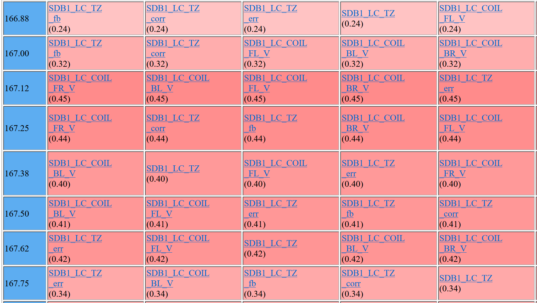
Figure 30: An example of bruco result webpage displaying, for each frequency bin (leftmost column), the most coherent channels sorted by decreasing coherence value, also represented by the red shade intensity. These data are from November 11, 2019. The large coherence detected at frequencies $155-170$ Hz triggered some further investigations of the noise [128].

Table 8: An excerpt (15 top lines) from top ranked channels’ summary with coherence greater than 0.3 for GPS time 1264319383 (2020/01/29 at 07:49:25 UTC).

Frequency [Hz]	Coherence	Type of channel
9.375	0.348	West arm transmitted power measurement
9.500	0.371	Angular correction of the last stage
		of wi payload suspension
13.375	0.308	Sensing signal measured at the dark fringe port,
		used to control optical cavity alignment
13.625	0.349	Same sensing signal
13.750	0.347	Same sensing signal
14.125	0.311	Same sensing signal
14.250	0.310	Same sensing signal
14.375	0.335	Same sensing signal
14.625	0.309	Same sensing signal
15.375	0.323	Same sensing signal
16.250	0.589	Longitudinal correction of the last stage
		of bs payload suspension
16.375	0.532	Same longitudinal correction
16.750	0.303	Same sensing signal
60.375	0.403	Calibration signal applied
		to the we test mass actuators

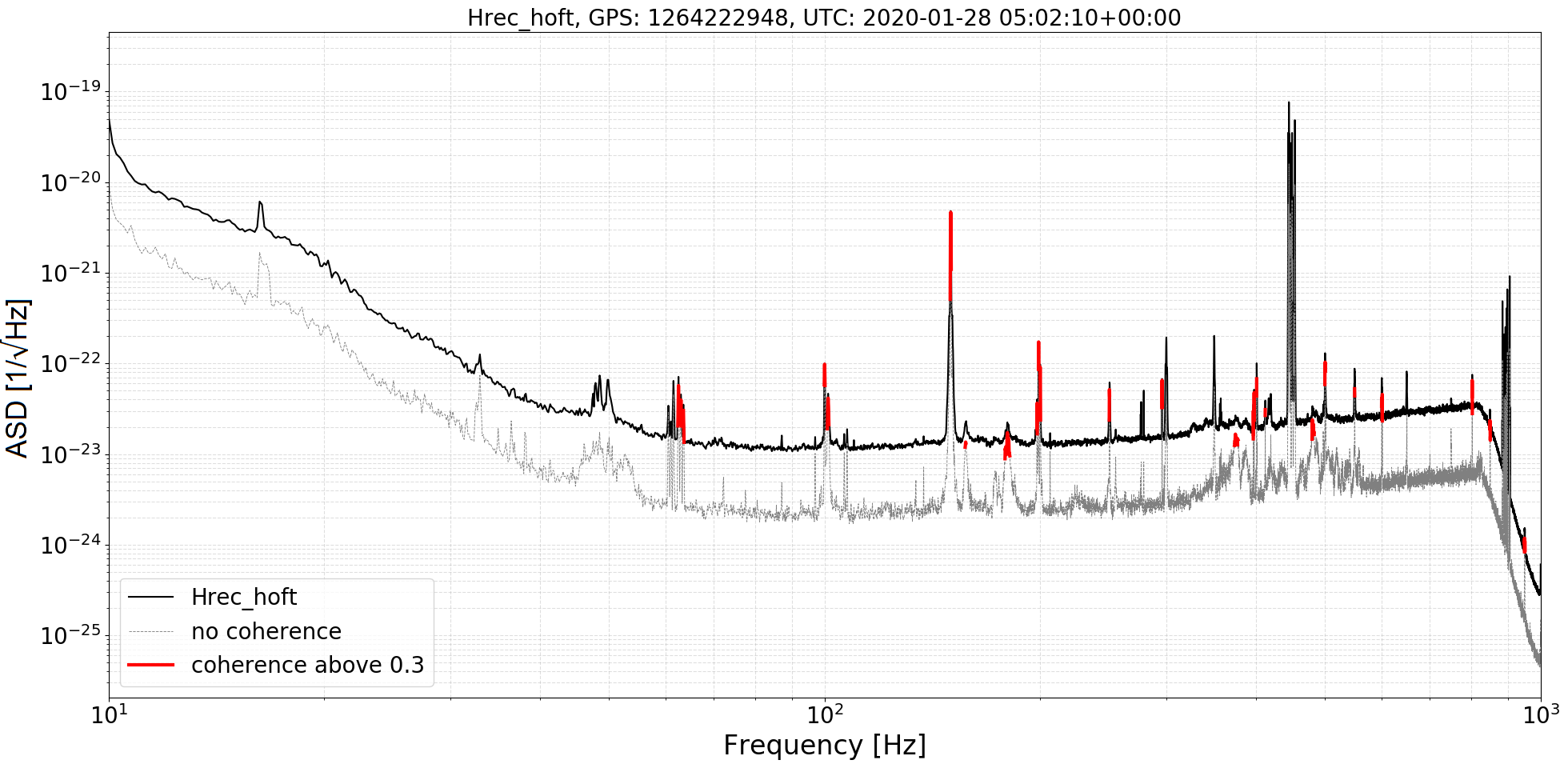
Figure 31: A bruco vim daily combined projection of the GW strain channel $h(t)$, showing coherences greater than 0.3 for the same GPS time 1264319383 (2020/01/29 at 07:49:25 UTC) as the previous plot.

A.4 MONET

monet computes the magnitude-squared coherence between a main channel (typically the DARM channel) and a list of other signals, that are constructed multiplying in the time domain a carrier signal and a set of modulating auxiliary channels to which a low-pass filter (with a typical cutoff frequency of a few Hz) is applied; the carrier signal can be a real channel or a simulated signal (e.g. a sinusoidal signal). Similarly to what is done with bruco, also with monet continuous science data segments of a specific time length $T$ are selected for all the channels to be investigated; then each data segment is resampled to a targeted output frequency ($f^{\rm out}$) and, finally, the magnitude-squared coherence is computed with Equation 6. For the analysis of O3 Virgo data we typically used a cutoff frequency of 5 Hz, $T=1200$ s and $f^{\rm out}$=1 kHz.

monet can be executed on demand, investigating dozens of auxiliary channels and spectral lines every single run. The outputs are organized in a directory structure:

• A main directory, whose name indicates the main channel, the initial gps time and the time length of the segment of data to be analysed.

• A secondary directory, named after the carrier signal used.

• Several sub-directories, one for each modulator channel.

The secondary directory contains an ascii table and a summary figure. The ascii table contains three columns: the frequency bins, the computed above-theshold coherence values for each bin (ordered from the lowest to the highest) and the corresponding modulator channels name. Figure 32 shows the MONET summary plot for the DARM channel during O3. Superimposed to the main channel’s asd there are red points marking the frequencies at which coherence above threshold is found with at least one auxiliary channel.

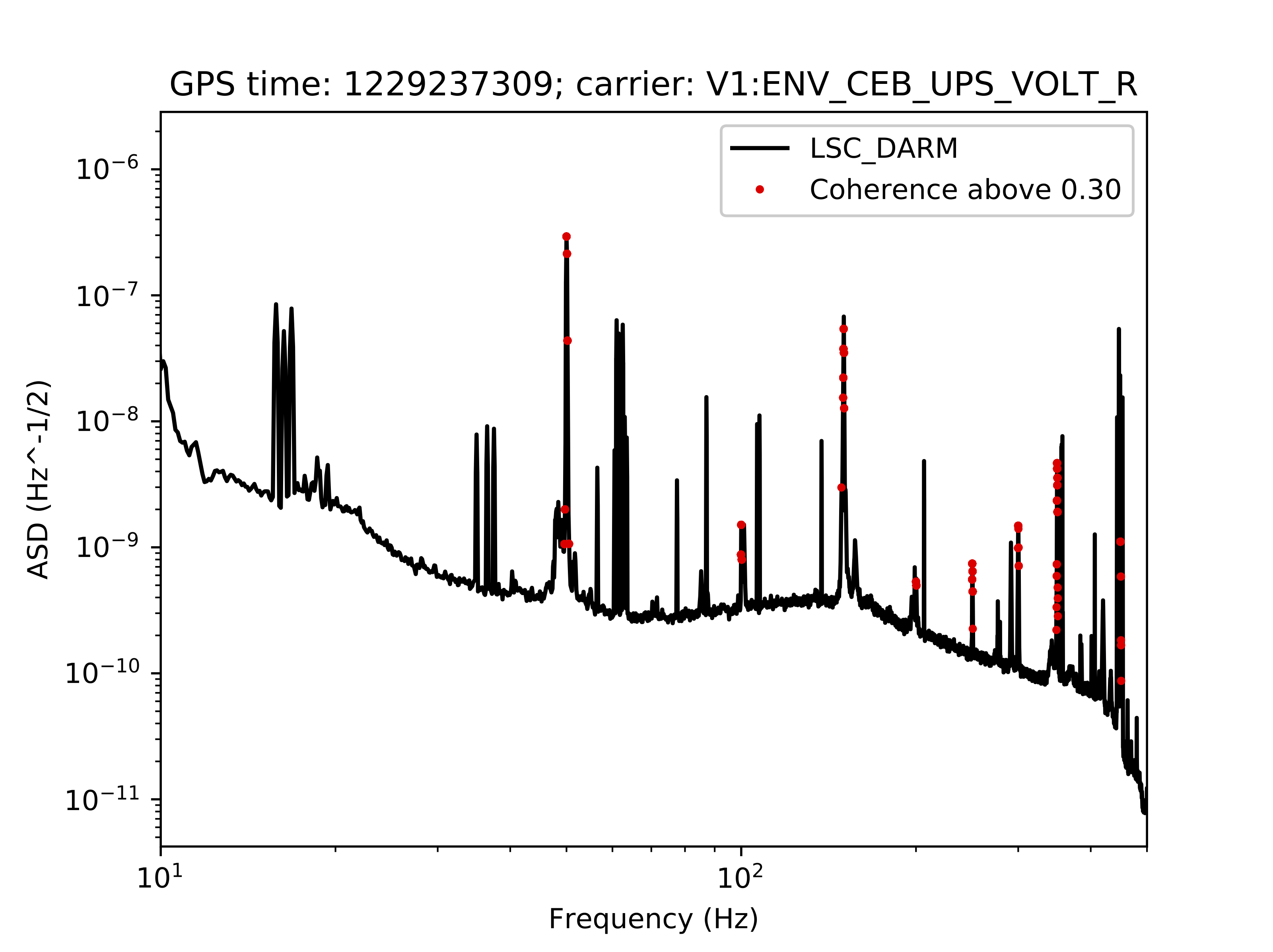
Figure 32: asd of the darm channel (in black), together with red points that mark the frequencies at which the coherence is above the threshold, fixed in this case at 0.3; the initial GPS time of the analysed data and the chosen carrier signal are indicated on the top of the figure.

In each sub-directory, a table and a plot are generated, in which the coherence values associated with the specific modulator channel for each frequency bin are reported; several other plots are also produced, in which the asd of the main channel is reported, together with the noise projection based on the coherence values, around the specific spectral lines to be investigated (see Figure 33).

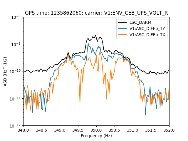
Figure 33: asd of the main channel (DARM) around the 350 Hz spectral line (in black), together with the noise projection, based on the coherence values obtained with the modulator channels ASC$\_$Diffp$\_$TY and ASC$\_$Diffp$\_$TX, in blue and orange respectively (these two channels are used to control the angular movement of the mirrors in the detector arms, to guarantee the proper ricombination of the laser beams at the beam splitter); the initial gps time of the analysed data and the chosen carrier signal are indicated on the top of the figure.

References

References

- [1] Abbott B et al. (LIGO Scientific Collaboration, Virgo Collaboration) 2016 Phys. Rev. Lett. 116 061102 (Preprint 1602.03837)
- [2] Aasi J et al. (LIGO Scientific Collaboration) 2015 Class. Quant. Grav. 32 074001 (Preprint 1411.4547)
- [3] Acernese F et al. (VIRGO) 2015 Class. Quant. Grav. 32 024001 (Preprint 1408.3978)
- [4] Akutsu T et al. 2021 Progress of Theoretical and Experimental Physics 2021 ISSN 2050-3911 05A102 (Preprint https://academic.oup.com/ptep/article-pdf/2021/5/05A102/38109702/ptab018.pdf) URL https://doi.org/10.1093/ptep/ptab018
- [5] Abbott B et al. (LIGO Scientific Collaboration, Virgo Collaboration) 2017 Phys. Rev. Lett. 119 161101 (Preprint 1710.05832)
- [6] Abbott R, Abbott T D, Abraham S, Acernese F, Ackley K et al. 2021 The Astrophysical Journal Letters 915 L5 URL https://doi.org/10.3847/2041-8213/ac082e
- [7] Abbott B et al. (LIGO Scientific Collaboration, Virgo Collaboration) 2019 Phys. Rev. X 9 031040 (Preprint 1811.12907)
- [8] Abbott R et al. (LIGO Scientific Collaboration, Virgo Collaboration) 2021 Phys. Rev. X 11 021053 (Preprint 2010.14527)
- [9] Abbott R et al. (LIGO Scientific, Virgo) 2021 (Preprint 2108.01045)
- [10] Abbott R et al. (The LIGO Scientific Collaboration, the Virgo Collaboration and the KAGRA Collaboration) 2021 arXiv e-prints (Preprint 2111.03606)
- [11] The LIGO Scientific Collaboration and The Virgo Collaboration 2021 Gravitational Wave Open Science Center (GWOSC) https://www.gw-openscience.org
- [12] Aasi J et al. (VIRGO) 2012 Class. Quant. Grav. 29 155002 (Preprint 1203.5613)
- [13] Aasi J et al. (LIGO Scientific, VIRGO) 2015 Class. Quant. Grav. 32 115012 (Preprint 1410.7764)
- [14] Accadia T, Acernese F, Alshourbagy M, Amico P, Antonucci F, Aoudia S, Arnaud N, Arnault C, Arun K G, Astone P and et al 2012 Journal of Instrumentation 7 3012
- [15] Aasi J et al. (LIGO Scientific Collaboration and Virgo Collaboration) 2015 Phys. Rev. D 91(2) 022004 URL https://link.aps.org/doi/10.1103/PhysRevD.91.022004
- [16] Dooley K L, Leong J R, Adams T, Affeldt C, Bisht A, Bogan C, Degallaix J, Gräf C, Hild S, Hough J, Khalaidovski A, Lastzka N, Lough J, Lück H, Macleod D, Nuttall L, Prijatelj M, Schnabel R, Schreiber E, Slutsky J, Sorazu B, Strain K A, Vahlbruch H, W?s M, Willke B, Wittel H, Danzmann K and Grote H 2016 Classical and Quantum Gravity 33 075009 URL http://stacks.iop.org/0264-9381/33/i=7/a=075009
- [17] The LIGO Scientific Collaboration 2015 Classical and Quantum Gravity 32 074001 URL http://stacks.iop.org/0264-9381/32/i=7/a=074001
- [18] Abbott B P, Abbott R, Abbott T D, Acernese F, Ackley K, Adams C, Adams T, Addesso P, Adhikari R X, Adya V B and et al 2017 Physical Review Letters 119 141101 (Preprint 1709.09660)
- [19] Abbott B P, Abbott R, Abbott T D, Acernese F, Ackley K, Adams C, Adams T, Addesso P, Adhikari R X, Adya V B and et al 2017 Physical Review Letters 119 161101 (Preprint 1710.05832)
- [20] Abbott B et al. (LIGO Scientific Collaboration and Virgo Collaboration) 2017 ApJ Lett. 848 L13
- [21] Abbott B et al. (LIGO Scientific Collaboration and Virgo Collaboration) 2017 ApJ Lett. 848 L12
- [22] Ballardin G et al. 2001 Review of Scientific Instruments 72 3643–3652 (Preprint https://doi.org/10.1063/1.1392338) URL https://doi.org/10.1063/1.1392338
- [23] Aisa D et al. 2016 Nuclear Instruments and Methods in Physics Research Section A: Accelerators, Spectrometers, Detectors and Associated Equipment 824 644 – 645 ISSN 0168-9002 frontier Detectors for Frontier Physics: Proceedings of the 13th Pisa Meeting on Advanced Detectors URL http://www.sciencedirect.com/science/article/pii/S016890021501092X
- [24] Accadia T, et al (The Virgo Collaboration) 2012 The AdV Technical Design Report Tech. Rep. VIR-0128A-12 URL https://tds.virgo-gw.eu/?call_file=VIR-0128A-12.pdf
- [25] F Travasso, on behalf of the Virgo Collaboration 2018 Journal of Physics: Conference Series 957 012012 URL https://doi.org/10.1088/1742-6596/957/1/012012
- [26] Acernese F et al. (Virgo Collaboration) 2019 Phys. Rev. Lett. 123(23) 231108 URL https://link.aps.org/doi/10.1103/PhysRevLett.123.231108
- [27] Harms J 2019 Living Reviews in Relativity 22
- [28] Allocca A, Bersanetti D, Casanueva Diaz J, De Rossi C, Mantovani M, Masserot A, Rolland L, Ruggi P, Swinkels B, Tapia San Martin E N, Vardaro M and Was M 2020 Galaxies 8 ISSN 2075-4434 URL https://www.mdpi.com/2075-4434/8/4/85
- [29] Fiori I, Paoletti F, Tringali M C, Janssens K, Karathanasis C, Menéndez-Vázquez A, Romero-Rodríguez A, Sugimoto R, Washimi T, Boschi V, Chiummo A, Cieślar M, De Rosa R, De Rossi C, Di Renzo F, Nardecchia I, Pasqualetti A, Patricelli B, Ruggi P and Singh N 2020 Galaxies 8 1–20
- [30] Acernese F et al. 2022 Submitted to Class. Quant. Grav., (Preprint 2203.04014)
- [31] Fiori I et al. 2020 Galaxies 8 ISSN 2075-4434 URL https://www.mdpi.com/2075-4434/8/4/82
- [32] Wipf, C SimulinkNb https://github.com/cwipf/SimulinkNb
- [33] Evans, M Optickle https://github.com/Optickle/Optickle/tree/Optickle2
- [34] L Naticchioni, for the Virgo Collaboration 2018 Journal of Physics: Conference Series 957 012002 URL http://stacks.iop.org/1742-6596/957/i=1/a=012002
- [35] Bader M K M 2021 Seismic and Newtonian noise modeling for Advanced Virgo and Einstein Telescope Ph.D. thesis Vrije Universiteit
- [36] Was M, Gouaty R and Bonnand R 2021 Class. Quantum Grav. 38
- [37] Hild S et al. 2009 Class. Quantum Grav. 26 055012
- [38] Fricke T et al. 2012 Class. Quantum Grav. 29 065005 (Preprint 0902.0381,)
- [39] Acernese F et al. 2022 Classical and Quantum Gravity 39 045006 (Preprint 2107.03294) URL https://doi.org/10.1088/1361-6382/ac3c8e
- [40] Estevez D, Mours B and Pradier T 2021 Classical and Quantum Gravity 38 075012 URL https://doi.org/10.1088/1361-6382/abe2da
- [41] Estevez D, Lagabbe P, Masserot A, Rolland L, Seglar-Arroyo M and Verkindt D 2021 Classical and Quantum Gravity 38 075007 URL https://doi.org/10.1088/1361-6382/abe2db
- [42] Graef Rollins J 2016 (Preprint 1604.01456)
- [43] Graef Rollins J 2014 Advanced LIGO Guardian: Overview and Coder’s Introduction Tech. Rep. G1400016 URL https://dcc.ligo.org/LIGO-G1400016/public
- [44] Buikema A et al. (aLIGO) 2020 Phys. Rev. D 102 062003 (Preprint 2008.01301)
- [45] Davis D et al. (LIGO) 2021 Class. Quant. Grav. 38 135014 (Preprint 2101.11673)
- [46] D Verkindt 2021 Advanced Virgo+ DataDisplay https://tds.virgo-gw.eu/ql/?c=16295
- [47] F Berni, F Carbognani, V Dattilo, F Gherardini, G Hemming, D Verkindt 2012 The Detector Monitoring System https://tds.virgo-gw.eu/ql/?c=9005
- [48] F Berni 2020 DMS help manual https://tds.virgo-gw.eu/ql/?c=15469
- [49] Abbott R et al. (LIGO Scientific Collaboration, Virgo Collaboration) 2020 Phys. Rev. D 102 043015 (Preprint 2004.08342)
- [50] Hemming G and Verkindt D 2016 Virgo interferometer monitor (vim) web user interface (wui) user guide Tech. Rep. VIR-0546A-16 URL https://tds.virgo-gw.eu/ql/?c=11869.
- [51] Verkindt D 2019 Proceedings of 54th Rencontres de Moriond, La Thuile URL http://moriond.in2p3.fr/download/proceedings-moriond-gravitation-2019.pdf
- [52] Frame Library https://git.ligo.org/virgo/virgoapp/Fr/-/tree/master/doc
- [53] The Virgo Collaboration 2021 PythonVirgoTools https://anaconda.org/conda-forge/pythonvirgotools
- [54] Davis M H A 1989 A Review of the Statistical Theory of Signal Detection (Dordrecht: Springer Netherlands) pp 73–94 ISBN 978-94-009-1185-7 URL https://doi.org/10.1007/978-94-009-1185-7_6
- [55] Abbott B P et al. 2020 Classical and Quantum Gravity 37 055002 URL https://doi.org/10.1088/1361-6382/ab685e
- [56] Aubin F et al. 2021 Class. Quant. Grav. 38 095004 (Preprint 2012.11512)
- [57] Dal Canton T, Nitz A H, Gadre B, Cabourn Davies G S, Villa-Ortega V, Dent T, Harry I and Xiao L 2021 Astrophys. J. 923 254 (Preprint 2008.07494)
- [58] Messick C, Blackburn K, Brady P, Brockill P, Cannon K, Cariou R, Caudill S, Chamberlin S J, Creighton J D, Everett R et al. 2017 Physical Review D 95 042001
- [59] Di Renzo F 2020 Characterisation and Mitigation of Non-Stationary Noise in Advance Gravitational Wave Detectors Ph.D. thesis Università di Pisa (Pisa, Italy) URL https://etd.adm.unipi.it/theses/available/etd-06192020-081853/
- [60] Kolmogoroff A 1941 The annals of mathematical statistics 12 461–463
- [61] Verkindt D 2019 Virgo spectrogram tools Tech. Rep. VIR-012A-19 URL https://tds.virgo-gw.eu/ql/?c=13835
- [62] Finn L S Gonzalez G and Sutton P J Rayleigh monitor (gaussianity test for ligo data) URL http://gallatin.physics.lsa.umich.edu/~keithr/lscdc/sutton_may01.html
- [63] Robinet F, Arnaud N, Leroy N, Lundgren A, Macleod D and McIver J 2020 SoftwareX 100620 ISSN 2352-7110 URL http://www.sciencedirect.com/science/article/pii/S2352711020303332
- [64] Brown J C 1991 The Journal of the Acoustical Society of America 89 425–434
- [65] Isogai T (Virgo, LIGO Scientific) 2010 J. Phys. Conf. Ser. 243 012005
- [66] Huang N E, Shen Z, Long S R, Wu M C, Shih H H, Zheng Q, Yen N C, Tung C C and Liu H H 1998 Proceedings of the Royal Society of London. Series A: mathematical, physical and engineering sciences 454 903–995
- [67] Huang N E, Shen Z and Long S R 1999 Annual review of fluid mechanics 31 417–457
- [68] Yang Y, Deng J and Wu C 2009 Analysis of mode mixing phenomenon in the empirical mode decomposition method 2009 Second International Symposium on Information Science and Engineering (IEEE) pp 553–556
- [69] Valdes G, O’Reilly B and Diaz M 2017 Classical and Quantum Gravity 34 235009
- [70] Longo A, Bianchi S, Plastino W, Arnaud N, Chiummo A, Fiori I, Swinkels B and Was M 2020 Classical and Quantum Gravity 37 145011
- [71] Li H, Li Z and Mo W 2017 Signal Processing 138 146–158
- [72] Chatterji S K 2005 The search for gravitational wave bursts in data from the second LIGO science run Ph.D. thesis Massachusetts Institute of Technology
- [73] Bianchi S, Longo A, Valdes G, González G and Plastino W 2021 arXiv preprint arXiv:2107.07565
- [74] Longo A, Bianchi S, Valdes G, Arnaud N and Plastino W 2022 Class. Quant. Grav. 39 035001 (Preprint 2112.06046)
- [75] Brun R and Rademakers F 1997 Nuclear Instruments and Methods in Physics Research Section A: Accelerators, Spectrometers, Detectors and Associated Equipment 389 81–86 ISSN 0168-9002 new Computing Techniques in Physics Research V URL https://www.sciencedirect.com/science/article/pii/S016890029700048X
- [76] Brun R et al. root-project/root: v6.18/02 URL https://doi.org/10.5281/zenodo.848818
- [77] Accadia T et al. 2012 Journal of Physics: Conference Series 363 012037 URL https://doi.org/10.1088/1742-6596/363/1/012037
- [78] Hemming, G and Piccinni, OJ NoEMi https://apps-online.virgo-gw.eu/noemi/docs/
- [79] The LIGO Scientific Collaboration and The Virgo Collaboration 2021 O3a Instrumental Lines https://www.gw-openscience.org/O3/o3aspeclines
- [80] Vajente G 2008 Analysis of sensitivity and noise sources for the Virgo gravitational wave interferometer Ph.D. thesis Scuola Normale Superiore (Pisa, Italy) chapter 8
- [81] Vajente, G BRUte force COherence https://github.com/gw-pem/bruco
- [82] Wąs, M 2019 PRCL bumps at 20 Hz and 40 Hz https://logbook.virgo-gw.eu/virgo/?r=44994
- [83] Aasi J et al. 2012 Classical and Quantum Gravity 29 155002 (Preprint 1203.5613)
- [84] Patricelli B & Cella G 2020 Tools for modulated noise study Tech. Rep. VIR-0575B-19 URL https://tds.virgo-gw.eu/?content=3&r=17154
- [85] Was, M & Patricelli, B 2019 Comment to Range variations and subtraction efficiency https://logbook.virgo-gw.eu/virgo/?r=47852
- [86] Di Renzo, F & Patricelli, B 2019 150 Hz side-bands https://logbook.virgo-gw.eu/virgo/?r=45974
- [87] Fiori, I, Paoletti, F, Singh, N & Patricelli, B 2018 Coherence analysis of 50Hz harmonics and calibration lines https://logbook.virgo-gw.eu/virgo/?r=42880
- [88] Fiori, I, Patricelli, B & Paoletti 2018 Comment to 1.5Hz sidebands https://logbook.virgo-gw.eu/virgo/?r=42630
- [89] Fiori, I, Was, M, Patricelli, B & Paoletti 2018 Demodulation noise at mains lines https://logbook.virgo-gw.eu/virgo/?r=42158
- [90] Fisher R P et al. 2021 SoftwareX 14 100677 URL https://www.sciencedirect.com/science/article/pii/S2352711021000224
- [91] The Gravitational-Wave Candidate Event Database (GraceDB) https://gracedb.ligo.org
- [92] The LIGO-Virgo Alert system (LVAlert) https://gracedb.ligo.org/documentation/lvalert.html
- [93] DQSEGDB web (protected) https://segments-web.ligo.org
- [94] Nitz A H, Dal Canton T, Davis D and Reyes S 2018 Phys. Rev. D98 024050 (Preprint 1805.11174)
- [95] Davies G S, Dent T, Tápai M, Harry I, McIsaac C and Nitz A H 2020 Phys. Rev. D 102 022004 (Preprint 2002.08291)
- [96] The LIGO-Virgo O3 public alerts https://gracedb.ligo.org/superevents/public/O3
- [97] The LIGO Scientific Collaboration and The Virgo Collaboration 2018 Data Quality Report User Documentation https://docs.ligo.org/detchar/data-quality-report
- [98] Litzkow M, Livny M and Mutka M 1988 Condor - a hunter of idle workstations Proceedings of the 8th International Conference of Distributed Computing Systems
- [99] S191124be GCN https://gcn.gsfc.nasa.gov/other/S191124be.gcn3
- [100] S200303ba GCN https://gcn.gsfc.nasa.gov/other/S200303ba.gcn3
- [101] Allen B 2005 Phys. Rev. D 71 062001 (Preprint gr-qc/0405045)
- [102] Nitz A H 2018 Class. Quant. Grav. 35 035016 (Preprint 1709.08974)
- [103] Nitz A H, Dent T, Dal Canton T, Fairhurst S and Brown D A 2017 Astrophys. J. 849 118 (Preprint 1705.01513)
- [104] Essick R, Mo G and Katsavounidis E 2021 Physical Review D 103 042003 (Preprint 2011.13787)
- [105] Riles K 2017 Modern Physics Letters A 32 1730035
- [106] Christensen N 2019 Reports on Progress in Physics 82 016903 (Preprint 1811.08797)
- [107] Aasi J, Abbott B P and Abbott T e a 2015 Physical Review D 91 022004 (Preprint 1410.8310)
- [108] The LIGO Scientific Collaboration, the Virgo Collaboration, the KAGRA Collaboration, Abbott R, Abe H, Acernese and et al 2022 arXiv e-prints arXiv:2201.00697 (Preprint 2201.00697)
- [109] Di Renzo F 2019 Wandering line jumping from 83.5 Hz to 108 Hz https://logbook.virgo-gw.eu/virgo/?r=46952
- [110] Fiori I, Swinkels B and Di Renzo F 2018 Line at 85 Hz now at 88 Hz and moving https://logbook.virgo-gw.eu/virgo/?r=43906
- [111] Mantovani, M et al 2017 84 Hz noise solved https://logbook.virgo-gw.eu/virgo/?r=38901
- [112] Fiori I and et al 2017 Comment to correlation of noise lines drifting in frequency with Env channels https://logbook.virgo-gw.eu/virgo/?r=38327
- [113] Rich Abbott et al. 2021 SoftwareX 13 100658 ISSN 2352-7110 URL https://www.sciencedirect.com/science/article/pii/S2352711021000030
- [114] The Virgo DetChar team 2021 ’Category 1’ (CAT1) data quality vetoes applied to the analysis of the O3 run Virgo data https://tds.virgo-gw.eu/ql/?c=16808
- [115] Adams T, Buskulic D, Germain V, Guidi G M, Marion F, Montani M, Mours B, Piergiovanni F and Wang G 2016 Class. Quant. Grav. 33 175012 (Preprint 1512.02864)
- [116] Klimenko S, Vedovato G, Drago M, Salemi F, Tiwari V, Prodi G A, Lazzaro C, Ackley K, Tiwari S, Da Silva C F and Mitselmakher G 2016 Phys. Rev. D 93(4) 042004 URL https://link.aps.org/doi/10.1103/PhysRevD.93.042004
- [117] Abbott B P, Abbott R, Abbott T D, Abraham S, Acernese F, Ackley K, Adams C, Adhikari R X, Adya V B, Affeldt C and et al 2019 Astrophysical Journal 875 161 (Preprint 1901.03310)
- [118] Mozzon S, Nuttall L K, Lundgren A, Dent T, Kumar S and Nitz A H 2020 Class. Quant. Grav. 37 215014 (Preprint 2002.09407)
- [119] Davis D and Walker M 2022 Galaxies 10 12
- [120] Cornish N J and Littenberg T B 2015 Class. Quant. Grav. 32 135012 (Preprint 1410.3835)
- [121] LIGO Scientific Collaboration and Virgo Collaboration 2019 GCN 26182 URL https://gcn.gsfc.nasa.gov/other/S191105e.gcn3
- [122] Schuster A 1898 Terrestrial Magnetism (Journal of Geophysical Research) 3 13
- [123] Acernese F, Amico P, Al-Shourbagy M, Aoudia S, Avino S, Babusci D, Ballardin G, Barillé R, Barone F, Barsotti L et al. 2005 Classical and Quantum Gravity 22 S1189
- [124] Welch P 1967 IEEE Transactions on Audio and Electroacoustics 15 70–73
- [125] Kokoszka P and Mikosch T 2000 Stochastic Processes and their Applications 86 49–79 ISSN 0304-4149 URL https://www.sciencedirect.com/science/article/pii/S0304414999000861
- [126] Di Renzo F and Sorrentino N 2020 BRiSTOL and RAGoUT: two tools for investigating noise stationarity and Gaussianity, for Detchar studies and Data Analysis Tech. Rep. VIR-0089A-20 URL https://tds.virgo-gw.eu/ql/?c=15203
- [127] Bendat JS and Piersol AG 2010 Random Data: Analysis and Measurement Procedures Wiley Series in Probability and Statistics (Hoboken, New Jersey, USA: Wiley) ISBN 978-0-470-24877-5
- [128] Di Renzo, F and Cieślar M 2019 Noise bumps between 155 and 170 Hz https://logbook.virgo-gw.eu/virgo/?r=47602