Realtime search for compact binary mergers in Advanced LIGO and Virgo’s third observing run using PyCBC Live

Abstract

The third observing run of Advanced LIGO and Advanced Virgo took place between April 2019 and March 2020 and resulted in dozens of gravitational-wave candidates, many of which are now published as confident detections. A crucial requirement of the third observing run has been the rapid identification and public reporting of compact binary mergers, which enabled massive followup observation campaigns with electromagnetic and neutrino observatories. PyCBC Live is a low-latency search for compact binary mergers based on frequency-domain matched filtering, which has been used during the second and third observing runs, together with other low-latency analyses, to generate these rapid alerts from the data acquired by LIGO and Virgo. This paper describes and evaluates the improvements made to PyCBC Live after the second observing run, which defined its operation and performance during the third observing run.

1 Introduction

The Advanced LIGO and Advanced Virgo gravitational-wave (GW) observatories conducted their first two observing runs, O1 and O2, between 2015 and 2017 (Aasi et al., 2015; Acernese et al., 2015; Abbott et al., 2018). From these two runs, over a dozen confident observations of binary black hole (BBH) mergers and one binary neutron star (BNS) merger were made (Abbott et al., 2017a, 2019a; Nitz et al., 2019a, b; Venumadhav et al., 2019; Zackay et al., 2021a; Venumadhav et al., 2020; Nitz et al., 2020b). The BNS merger, GW170817, was observed within a minute of the data being recorded, was associated with a gamma ray burst (Abbott et al., 2017b) and was subsequently followed up by a large number of observatories spanning the whole electromagnetic (EM) spectrum (Abbott et al., 2017c). Without the realtime identification and localization of GW170817 as a merging pair of neutron stars, these observations would not have been possible.

The third observing run of Advanced LIGO and Advanced Virgo, O3, began in April 2019 and ended in March 2020. Thanks to hardware improvements in the detectors, the ranges for compact binary mergers were expected to increase by 6–85% with respect to O2, depending on the source type and detector, with the largest improvement expected for Virgo (Abbott et al., 2018). The sensitive volume of the run was then predicted to be $3.3\times 10^{6}$ Mpc³ yr for BNS mergers, and $3.4\times 10^{8}$ Mpc³ yr for BBH mergers. With this unprecedented sensitivity, we expected to observe up to $\approx 40$ BBH mergers, up to $\approx 10$ BNS mergers, and potentially make the first observation of a neutron-star-black-hole (NSBH) merger. Indeed, dozens of candidates from O3 have been uploaded to GraceDB and announced on the Gamma-ray Coordinates Network (GCN). Four such candidates have been published as notable compact binary mergers so far (Abbott et al., 2020a, b, c, d). Many more confident detections from the first half of O3 have also been presented in the GWTC-2 (Abbott et al., 2021a) and 3-OGC (Nitz et al., 2021) catalogs. O3 was the first observing run in which three observatories operated for the full duration of the run, increasing the observing duty cycle of the network, reducing the uncertainty in the sky location of observed events and therefore maximizing the chance of making a multi-messenger observation (Abbott et al., 2018). Rapid processing of data from all three observatories was therefore a crucial requirement.

PyCBC Live, first introduced by Nitz et al. (2018), is one of several search codes analysing the data in realtime to observe compact binary mergers, other analyses being GstLAL (Messick et al., 2017; Sachdev et al., 2019), MBTA (Adams et al., 2016; Aubin et al., 2021), SPIIR (Hooper et al., 2012; Chu, 2017; Chu et al., 2020) and the generic-transient search cWB (Klimenko et al., 2016). Having multiple analyses provides for redundancy, both in terms of the possibility that one of the analysis fails for any reason, and in terms of the independent methodology that each of these analyses applies to identify compact binary mergers. PyCBC Live is based on the more general PyCBC software package (Nitz et al., 2020a) and uses a precalculated bank of compact binary merger waveform models combined with matched filtering in the frequency domain (Allen et al., 2012; Babak et al., 2013). PyCBC Live has been instrumental in many of the GW observations to date, both in O2 (Abbott et al., 2017d, e, f, a) and O3 (Abbott et al., 2020b, a, d).

In this paper we describe the improvements that have been made to PyCBC Live in preparation for, and during, O3. Specifically, we discuss the new techniques that (i) enabled the simultaneous and symmetric analysis of data from three observatories, and the reliable assessment of the statistical significance of observed candidates, (ii) improvements in the handling of instrumental transients, (iii) an updated technique to detect signals in data from a single detector and (iv) a method to rapidly infer the nature of the compact objects involved in a candidate merger. We then evaluate the effect of these improvements in terms of search sensitivity by simulating compact binary signals in Gaussian data at the design sensitivity of advanced GW detectors, as well as in real O3 data from Advanced LIGO and Advanced Virgo. We also evaluate the accuracy of the source classification method and the effect of these improvements on the latency of the produced candidates using O2 data.

2 New methods for the third observing run

This section describes the new methodology that was used or developed in PyCBC Live during O3. Each subsection describes changes to a specific aspect of the analysis, and subsections are ordered so as to follow the data flow through the pipeline as much as possible.

2.1 Search space and template bank

Although it is an improvement to the configuration of PyCBC Live rather than the code itself, we begin by describing the search space and template bank adopted during O3, as a reference for future work.

The bank covers the same mass, spin and waveform duration space as that proposed by Dal Canton & Harry (2017) and previously adopted during O2. The same waveform models are also employed: TaylorF2 (Buonanno et al., 2009; Bohé et al., 2013) for BNS and low-mass NSBH templates, and a reduced-order frequency-domain version of SEOBNRv4 (Bohé et al., 2017; Pürrer, 2014) for BBH and heavy NSBH templates.

However, the O3 bank utilises a template placement method based on an optimized hybrid geometric-random approach (Roy et al., 2017, 2019, 2018) which is more efficient than the “manual” combination of geometric and stochastic methods used for the O2 bank (Dal Canton & Harry, 2017) in the sense that the obtained bank is $\sim 25$% smaller and can be produced much faster. As a result, the O3 bank is only 13% larger than the O2 bank, despite the increased sensitivity of the detectors.

2.2 Improved rejection of instrumental transients

Loud instrumental transients in GW data (glitches) which last much less than a second can corrupt the results of transient searches on a time scale much longer than the glitch itself (Dal Canton et al., 2014). In particular, due to the relatively long-lasting impulse response of the various filters involved in the SNR calculation, loud glitches can cause the SNR time series for a given template to cross the trigger-generation threshold many times over several seconds. The resulting high-SNR triggers then dominate over quieter triggers from the underlying stationary noise and possible astrophysical signals, effectively blinding the search for the entire duration of the impulse response of the filters. In early O3, this issue appeared prominently in the results of PyCBC Live as occasional gaps in the production of triggers from a given detector, lasting from a few seconds to several tens of seconds, depending on the glitch.

A simple and widely-used solution to this problem, called gating, consists of windowing out the GW strain data for a short window centered on the glitch prior to matched filtering (Abbott et al., 2016; Usman et al., 2016; Sachdev et al., 2019). PyCBC offline searches already implement this method by detecting glitches as loud excursions in the whitened strain, and then multiplying the data with the complement of a Tukey window centered on the glitch time. We adopted the same algorithm in PyCBC Live during O3. We used a threshold of $50\sigma$ on the absolute value of the whitened strain time series as a glitch detector. Each detected glitch was gated with a symmetric complemented Tukey window, configured to have 0.5 s of central zeroes and 0.25 s of smooth taper on both sides. This approach significantly reduced the impact of high-SNR non-Gaussian transient noise with no visible impact on the latency of the analysis. The chosen gating duration is justified because many high-SNR glitches tend to be shorter than 1 s (Davis et al., 2021) and significantly longer gates might cause more damage to downstream stages of the analysis than the glitch itself. A fixed duration also removes the need to estimate the duration of the glitch, which is nontrivial due to the impulse response of the whitening filter, often longer than the glitch itself. Nevertheless, a fast gating procedure which more accurately identifies the time-frequency extent of a glitch could be beneficial in the future.

Another improvement inherited from PyCBC’s offline search during O3 was the inclusion of the high-frequency sine-Gaussian discriminator in the ranking of single-detector triggers. The discriminator, described in Nitz (2018), exploits the fact that most compact binary mergers induce a negligible amount of signal power at frequencies higher than the ringdown of the dominant quadrupole mode. By measuring the excess power at the time of peak signal amplitude, and at various frequencies above the ringdown, a $\chi^{2}$ statistic is constructed and used to reweight the single-detector trigger ranking statistic. The discriminator is most effective at preventing glitches from triggering high-mass templates with final frequencies of $\approx 100$ Hz or less, hence it increases the search sensitivity to high-mass black hole mergers. We adopted the same implementation of the discriminator used by PyCBC’s offline search with a negligible impact on PyCBC Live’s latency.

2.3 Inclusion of Virgo in the coincident search

Advanced Virgo began operating in conjunction with the LIGO observatories in the last few months of O2, when its sensitivity was typically $1/4$ to $1/3$ that of the LIGO instruments. Despite the smaller sensitivity, the inclusion of Virgo markedly improved the localization of important candidates, such as GW170817 (Abbott et al., 2017a). However, Virgo’s contribution to the overall network sensitivity was limited, as quantified by its integrated BNS observed time-volume of $4\times 10^{3}$ Mpc³ yr compared to $5\times 10^{5}$ Mpc³ yr for LIGO-Hanford. Hence, in order to produce candidate events, the PyCBC Live analysis introduced in Nitz et al. (2018) relied on a simple coincident detection between the two LIGO observatories only. Additional detectors were analyzed by PyCBC Live for the purpose of improving the rapid spatial localization, but they did not contribute to the significance of candidates, and they could not produce candidates in coincidence with one of the LIGO detectors.

However, as the relative sensitivities of the instruments within the global GW network become comparable, each instrument’s contribution to the overall sensitivity also increases. In the coming years, the Virgo observatory may approach $60$–$80\%$ of the LIGO detector sensitivities, limited primarily by its shorter arm length (Abbott et al., 2018). In addition, new instruments will be joining the global network: KAGRA (Somiya, 2012; Aso et al., 2013; Akutsu et al., 2020), which conducted its first observing period shortly after the end of O3, and LIGO-India (Iyer et al., 2011), scheduled to begin operation in the mid 2020’s (Abbott et al., 2018). The higher network sensitivity comes about from two sources: (1) improvement in overall network uptime due to overlap between instruments live time, and (2) improvement in detection confidence (reduction of the false-alarm rate) from additional detectors. Hence, in order to start exploiting the benefits of a larger and more symmetric network, the PyCBC Live analysis has been modified for the O3 run.

In its O3 configuration, PyCBC Live correlates the full bank of template waveforms with data from all operating detectors. Then for each detector pair, we independently perform the same double-coincident analysis used for LIGO-Hanford and LIGO-Livingston during O2. When a pair of detectors labelled $A$ and $B$ observe a coincident candidate, a false-alarm rate $\mathcal{F}_{AB}$ is computed using time-shifted analysis of these two detectors’s data, as done in O2. The $\mathcal{F}_{AB}$ estimate is local, using only the last $5$ hr of data, and therefore tracks possible slow changes in the properties of the detector noise. At times when $A$ and $B$ are the only operating detectors, any candidate events are then submitted directly to GraceDB with false-alarm rate $\mathcal{F}_{AB}$, the analysis being effectively identical to O2. However, if additional detectors are observing at the time of the candidate ($C$, $D$…), a combined false-alarm rate is computed as follows.

First, we correct the double-coincident false-alarm rate to include the trials factor associated with the choice between possible detector pairs,

$$\mathcal{F}^{\rm tf}_{AB}={N\choose 2}\mathcal{F}_{AB}$$ (1)

where $N$ is the number of detectors that can generate double coincidences at the time of the candidate. If multiple instrument pairs generate coincident candidates from the same transient, we select the candidate having the lowest false-alarm rate. If tied, we select the candidate with the largest ranking statistic value.

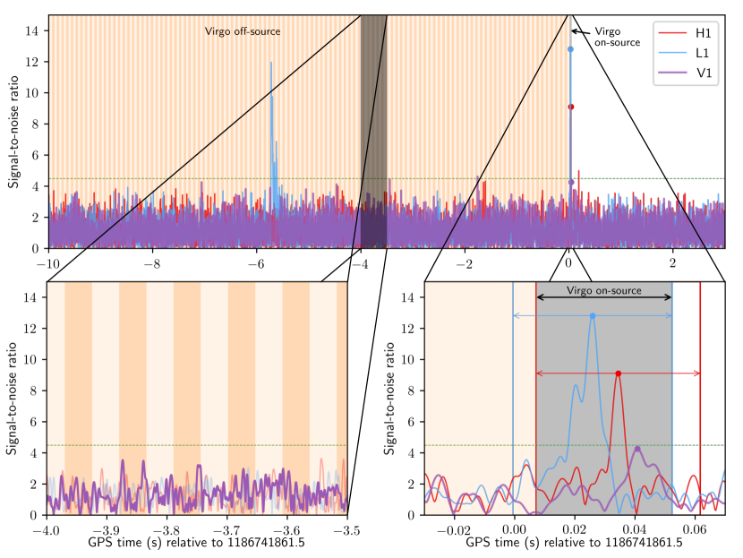
Figure 1: Visualization of the process used by PyCBC Live to generate a three-detector coincident candidate. In this example, the LIGO-Hanford and LIGO-Livingston SNR time series (red and blue curves) have two nearby peaks above the trigger-generation threshold (dashed horizontal line). The coincident peaks then produce a Hanford-Livingston coincident candidate. The window of possible signal arrival times at Virgo (on-source region, dark gray in the bottom-right panel) is calculated using the Hanford and Livingston triggers, as indicated by the horizontal arrows. The Virgo SNR time series is calculated (violet, thick curve) and searched for its maximum within the on-source region. Once the maximum is identified, its statistical significance is determined by comparing it to the maxima occurring in the off-source intervals (vertical stripes of alternating color in the top and bottom-left panels).

Then, using the template of the selected candidate, we calculate the signal-to-noise ratio (SNR) time series for the remaining detectors, which we call followup detectors, and then use this time series to obtain a p-value for each followup detector. Assuming a plane GW traveling at the speed of light, and using the arrival times estimated at detectors $A$ and $B$, an on-source time interval of possible arrival times is determined at each followup detector. The maximum SNR within the on-source interval is identified. Next, $150$ s of data immediately before the on-source window, called off-source data, are segmented into $N_{\rm off}$ intervals of the same duration as the on-source data (Figure 1). The maximum SNR in each off-source interval is calculated, and the number $M_{\rm off}$ of off-source intervals having a SNR larger than the on-source SNR is used to compute the p-value,

$$p_{C}=\frac{1+M_{{\rm off,}C}}{1+N_{\rm off}},$$ (2)

where $C$ labels the followup detector(s). This is the probability of producing a SNR as large as the one observed under the assumption that detector $C$’s data contains only noise. Such a p-value is produced for each followup detector ($p_{C}$, $p_{D}$…). In addition, we obtain the p-value for the original double-coincident candidate as

$$p_{AB}=1-\exp\left[-T_{\rm live}\mathcal{F}^{\rm tf}_{AB}\right]$$ (3)

where $T_{\rm live}=4.38$ hr (0.005 yr) is a fiducial livetime used to convert false-alarm rates to p-values. Its value is close to the amount of single-detector data stored for background computation, and also close to the minimum inverse false-alarm rate required for uploading a candidate to GraceDB. The two-detector p-value $p_{AB}$ is then combined with the followup detector p-value $p_{C}$ using an adaptation of Fisher’s method (Fisher, 1970):

$$p_{ABC} = \mathcal{P}\left(2,-\ln(p_{AB}p_{C})\right)=$$ (4)

$$= p_{AB}p_{C}\ \left[1-\ln(p_{AB}p_{C})\right]$$ (5)

where $\mathcal{P}(\cdot,\cdot)$ is the regularized gamma function. (For more than one followup detector, our algorithm performs this combination iteratively.) Next, we convert back to a false-alarm rate,

$$\mathcal{F}_{ABC}=-T^{-1}_{\rm live}\ln(1-p_{ABC}).$$ (6)

For the final significance, we additionally select the minimum of the original two-detector and multi-detector false-alarm rates,

$$\mathcal{F}=2\min\{\mathcal{F}^{\rm tf}_{AB},\mathcal{F}_{ABC}\},$$ (7)

where the trials factor of 2 accounts for this additional choice. This procedure produces a self-consistent rate of false alarms under the null hypothesis, and assuming time-invariance of the noise for the collected background. The latter assumption may be violated if one or more detectors rapidly change to a new operating state, hence the desire is to use as short a background collection time as possible to track these changes.

We now apply the above equations to two limiting examples to illustrate possible results in practice. We first consider the case of a nearby source and $3$ detectors with similar sensitivities. The source produces a very loud coincidence in detectors $A$ and $B$ as well as a very high SNR in detector $C$, where by “very loud” we mean that the SNR is higher than any background it is compared to. In this case we obtain the lower bound $(\mathcal{F}_{AB})^{-1}>100$ yr, determined by the amount of data chosen to estimate the double-coincident background. Assuming an on-source window of $40$ ms for detector $C$, we also have the upper bound $p_{C}\lesssim 2.7\times 10^{-4}$. Then, using the above formalism, we obtain $\mathcal{F}^{-1}\gtrsim 3500$ yr. Consider now a similar situation, but the sensitivity of detector $C$ is so low that the signal is completely undetectable in its data, leading to $p_{C}\approx 0.5$. This results in the bound $\mathcal{F}^{-1}\gtrsim 17$ yr, weaker than the original bound on $\mathcal{F}_{AB}$ due to the combined effect of the trials factors and a detector with low sensitivity. Nevertheless, the limit is still well below the threshold required for a public alert and for considering the candidate worthwile of additional astronomical observations. In these examples, we emphasized that the resulting false-alarm rates are to be understood as upper limits, as they are limited by the amound of data chosen to estimate the background, and not by the SNR of the candidate. The limits can be lowered by using more data, but this comes at the risk of increasing our sensitivity to sudden changes in the noise properties of the detectors.

Note that the on-source SNR in the followup detectors is not required to cross any threshold. Hence, this method naturally allows even weak signals in the followup detectors to increase the significance of the original coincident candidates. However, a potential limitation of the method is represented by the implicit assumption that all detector pairs are equally likely to produce an initial double coincidence in response to a signal. This leads to the trials factor in Eq. 1 being potentially very large: for a network of 3 detectors, such as during O3, the total trials factor can be as high as 6. As additional observatories join the network, the trials factor will grow rapidly and this method may not offer a sensitivity close to optimal. One way to reduce the trials factor would be to use the local sensitivity of each instrument to predict the instrument pair(s) most likely to produce a detection, and only consider those pair(s) in the calculation of the combined false-alarm rate. An alternative strategy for a heterogeneous network could be modifying Eq. 1 to weight each detector pair in a way that accounts for different sensitivities. Finally, the iterative application of Fisher’s method described above could be replaced by a single application of the method to all available p-values. Although the two approaches produce p-values well within a factor of 2 in the case of 2 followup detectors (i.e. a LIGO-Virgo-KAGRA network), a single combination may lead to a higher sensitivity in the case of a 5-detector network.

2.4 Identification of signals in a single detector

During an observation run, there will undoubtedly be times during which a detector cannot operate, or is affected by severe nonstationary or transient noise. Moreover, all detectors are blind to signals coming from certain positions in the sky, and these positions are detector-dependent. Therefore, a non-negligible fraction of signals are unable to produce coincident triggers in two or more detectors (Callister et al., 2017; Nitz et al., 2020b). By chance, two events that were very promising targets for EM followup observation were first identified as single-detector triggers: GW170817, initially seen as a single-detector trigger in LIGO Hanford due to a large glitch affecting LIGO Livingston (Abbott et al., 2017a) and GW190425, observed by LIGO Livingston and Virgo, but too weak to be detectable in Virgo (Abbott et al., 2020a). In cases like these, we have a single-detector trigger and no coincidence. We cannot rely on the usual robust time-slide approach to establish the false-alarm rate of the trigger, and an alternate method is required. We note and caution that formally, the false alarm rate can only be assigned with confidence to be less than once per livetime for single-detector candidates. Beyond this point, extrapolation is used in order to generate low-latency alerts. If the detector noise changes in unexpected ways, the extrapolation may become invalid and the rate of false positives for single-detector candidates may no longer match an extrapolated false alarm rate.

During O2, PyCBC Live relied on a simple algorithm to identify single-detector candidates based on a pre-determined ranking statistic threshold, and a set of signal-consistency cuts, which were chosen based on early detector data. The algorithm was only active when a single detector was observing. We improve on this method by implementing a complete ranking statistic and procedure for extrapolating the false-alarm rate. We further increase the coverage of our single-detector search by allowing it to operate during times when multiple detectors are observing, as the relative sensitivities of two detectors may imply that a signal can only be seen in one of them.

Our single-detector trigger ranking statistic is the usual reweighted SNR (Usman et al., 2016),

$$\hat{\rho}=\left\{\begin{array}[]{lR}\rho\left[(1+(\chi^{2}_{r})^{p/2})/2\right]^{-1/p}&if $\chi^{2}_{r}>1$\\ \rho&if $\chi^{2}_{r}\leq 1$\end{array}\right.,$$ (8)

where $\rho$ is the matched-filter SNR, $\chi_{r}^{2}$ is the time-frequency discriminator described by Allen (2005), and $p$ is an index set to the usual value of $6$. Note that the same $\hat{\rho}$, calculated for each detector and complemented by other terms, also defines the ranking statistic of coincident triggers.

As we do not have a coincident trigger to corroborate the evidence of a signal, we must apply strict cuts in order to remove triggers which are likely to be glitches. Therefore we remove any trigger with $\hat{\rho}<9$ or $\chi_{r}^{2}>2$, which comes at the cost of possibly removing some signals that are not particularly well matched by the templates. We further restrict the calculation to triggers coming from a template describing a system with a non-negligible mass remaining outside of the final black hole. By doing so, we ignore many of the templates which match best to common types of glitch in the LIGO detectors, as well as focus on the templates corresponding to sources which are most interesting for potential generation of EM counterpart emission. Applying the remnant mass equation from Foucart et al. (2018) to all templates in our bank, we find that this mass is negligible for templates with duration shorter than $\sim 7$ s. Therefore, we prevent triggers associated with shorter templates from generating single-detector candidates.

The probability distribution of $\hat{\rho}$ for triggers associated with detector noise is expected to follow a falling exponential, as described in Davies et al. (2020),

$$\mathrm{p}(\hat{\rho}|\textrm{noise})=\left\{\begin{array}[]{lR}\alpha\exp\left[-\alpha(\hat{\rho}-\hat{\rho}_{th})\right]&if $\hat{\rho}>\hat{\rho}_{th}$\\ 0&if $\hat{\rho}\leq\hat{\rho}_{th}$\end{array}\right.,$$ (9)

where $\hat{\rho}_{th}$ is a threshold on the reweighted SNR, and $\alpha$ is the fit coefficient. Given the selection cuts defined above, we find empirically that this model describes the detector noise very well.

For each detector, we fit Eq. 9 to the triggers from a day’s worth of data and record the fit coefficient, combining these over a longer period of time. Then, during PyCBC Live’s operation, we can use this coefficient to estimate the false-alarm rate for each single-detector trigger that passes the selection cuts described above. In general, this fit could be performed separately for each template, but we instead choose to perform the fitting in five bins which are spaced logarithmically in template duration. This choice allows us to group many templates which behave similarly in the presence of noise, and hence increase the number of triggers available for the fit.

Noise in ground-based GW detectors is affected by slowly-varying environmental processes, like weather, and by commissioning activities that change the detector properties over time. Therefore, the statistical properties of the noise are time-dependent, and the fit coefficients for each bin will also vary over time. To account for this variation, we combine the daily fit values in one of two ways. The maximum likelihood choice of $\alpha$ is proportional to the inverse of the mean $\hat{\rho}$ for each template (Davies et al., 2020), and so we can take the mean of $\alpha^{-1}$ over the different days, weighted by the number of triggers from each day in order to combine these fits. Alternatively, we could take a low percentile of the $\alpha$ distribution over different days. This would lead to a much more conservative estimate of the false alarm rate. In our case we use the $5^{\mathrm{th}}$ percentile value, and call this the conservative fit coefficient. This conservative choice would be used for issuing alerts during future observing runs, as it would reduce the number of false alarms compared to the use of the mean coefficient.

We see the variation and combination of the trigger fit coefficient in Figure 2, where the fit coefficient in each template duration bin is plotted for each day of July 2017, along with the mean and conservative combinations.

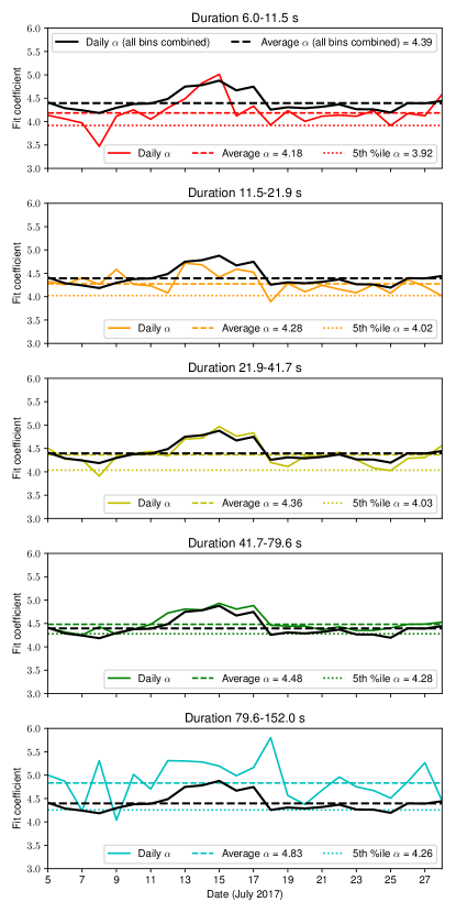
Figure 2: Fit coefficients $\alpha$ calculated daily for triggers from a month of O2 LIGO Hanford data which meet the $\hat{\rho}$, $\chi^{2}_{r}$ and template duration cuts as described in the text. One plot is given for each template duration bin, and longer templates generally have fewer triggers at high $\hat{\rho}$, so the fit coefficients are larger. The dashed and dotted lines show the mean and conservative combinations of the fit coefficients, used to estimate the false-alarm rates of future single-detector candidates, and the black lines are for comparison to the fit values if they were not separated into different duration bins.

To calculate the expected rate of louder triggers, as well as the trigger distribution of Eq. 9, we must estimate the overall rate of triggers. This is done by simply counting the triggers which pass the specified thresholds in the daily fits, and for the mean fit, this is simply an addition of the daily trigger counts. For the conservative fit choice, we choose the $95^{\mathrm{th}}$ percentile daily trigger count and multiply by the number of days over which the fit smoothing is performed.

Using the originally recorded trigger from LIGO Hanford, and the conservative fit values calculated from the O2 data from July 2017, we estimate the single-detector trigger false alarm rate in LIGO Hanford of GW170817 to be 1 per $\mathcal{O}(10^{9})$ yr. If we choose the mean fit combination, then the estimated false alarm rate would be 1 per $\mathcal{O}(10^{11})$ yr.

2.5 Source classification

Source classification between different possible types of coalescing compact binary is an important element in generating followup alerts for EM or other counterpart signals. For the O3 run, four astrophysical source types: BNS, BBH, NSBH and MassGap, were considered (LIGO Scientific and Virgo Collaborations, 2019). The desired classification designated every object with a mass below $3\,M_{\odot}$ as a neutron star, every object with mass above $5\,M_{\odot}$ as a black hole, and every object between these two thresholds as a MassGap object; any binary containing one or more MassGap components was then considered as MassGap. Accurate classification in low latency is a considerable challenge: in general for lower-mass binaries, only the chirp mass

$$\mathcal{M}=\frac{(m_{1}m_{2})^{3/5}}{(m_{1}+m_{2})^{1/5}}$$ (10)

can be precisely measured, while the mass ratio has large uncertainty. In addition, typically search pipelines report only a point estimate of redshifted component masses, and these template masses may be subject to systematic biases relative to the true source-frame component masses (see e.g. Biscoveanu et al., 2019). During O3, astrophysical source classification for PyCBC Live candidates was performed by the LIGO/Virgo rapid alert infrastructure using a “hard cuts” method, which assigns Boolean weights (either $1$ or $0$) to the different source types based on component mass cuts applied to the reported search template. The fact that this method neglects uncertainties in component masses and does not account for any systematic error in mass recovery suggests the potential for improvement (compare Kapadia et al., 2020).

A new approach developed during the later part of the O3 run, which will be described in detail in Villa-Ortega et al. (2022, in preparation), uses the chirp mass recovered by the search pipeline as input, and implicitly assumes a uniform density of candidate signals over the plane of component masses $m_{1}$, $m_{2}$. These source-frame masses are constrained to the interval $1\,M_{\odot}<m<45\,M_{\odot}$, where the lower bound is the lower limit on the template bank mass space described in the Section 2.1, and the upper bound is chosen based on BBH population studies up to the first half of the third observing run, O3a (Abbott et al., 2019b, 2021b). Constraining the chirp mass to be within a confidence interval around a point estimate derived from the search template determines an allowed region in the $m_{1}$–$m_{2}$ plane; we then estimate the probability that a candidate belongs to each source category to be directly proportional to the area of the allowed region satisfying the criteria for the given category. The output of the method for a given event is a list of probabilities $\left\{P_{\rm BNS},P_{\rm NSBH},P_{\rm MG},P_{\rm BBH}\right\}$ summing to unity.

To compute these areas we require accurate estimates of the candidate chirp mass in the source frame, thus we apply a correction for the bias caused by cosmological redshift. For this correction we use estimates of the luminosity distance and its uncertainty derived from the effective distances (Allen et al., 2012) of the trigger(s) comprising the event:

$$\tilde{D}_{\rm L} = \mathrm{const}\cdot\min(D_{\rm eff}),$$ (11)

$$\tilde{\sigma}_{{D}_{\rm L}} = \tilde{D}_{\rm L}\cdot\mathrm{const}\cdot\rho_{\rm coinc}^{-p},$$ (12)

where $\min(D_{\rm eff})$ is the minimum effective distance over all triggers obtained for a given coincident or single-detector event, and the constants of proportionality and power law exponent $p$ may be derived from a fit to previously obtained three-dimensional localizations produced by the BAYESTAR pipeline (Singer & Price, 2016) for PyCBC Live events. Although in most cases the uncertainty in the source chirp mass is expected to be dominated by the redshift (distance) uncertainty, we combine this with a nominal, small uncertainty of 1% in the detector-frame chirp mass relative to the value recovered by the search pipeline.

Our approach may be compared to the ‘ellipsoid-based’ method outlined in Chatterjee et al. (2020). The ellipsoidal error region considered there accounts for expected uncertainties in the recovered masses and spins in the limit of Gaussian detector noise and high SNR (though without attempting to correct for the source redshift). It was also noted there that the actual recovery of parameters other than $\mathcal{M}$ by search pipelines was subject to significantly larger systematic error, motivating an alternative machine learning based method. Our approach is simpler in that we effectively consider the uncertainties in such parameters to be infinitely large: we leave improvements to this approximation to future work.

2.6 Search for maximum-SNR template

The rapid spatial localization of GW alerts performed by BAYESTAR (Singer & Price, 2016) relies on the knowledge of the template that maximizes the likelihood assuming stationary Gaussian noise (or equivalently, the template that maximizes the network matched-filter SNR) for a given candidate. The template is usually taken directly from the candidate produced by the low-latency search. However, when a search like PyCBC Live generates a candidate in response to an astrophysical signal, it includes both astrophysical priors and the presence of nonstationary and non-Gaussian noise features into the significance of the candidate. Hence, the template immediately associated with a candidate will not necessarily maximize the network SNR under the assumption of stationary Gaussian noise. The sparseness of the template bank will generally also drive the reported template parameters away from the maximum SNR. This could in principle introduce biases in the rapid spatial localization, and more generally affect any low-latency result which uses the mass and/or spin parameters of the search template, such as the source classification we described above in Section 2.5. See Biscoveanu et al. (2019); Chatterjee et al. (2020) for investigations of such possible biases.

In order to remove some of the sources of these biases, we developed a followup process that starts after PyCBC Live reports a candidate to GraceDB. The process reanalyzes a short amount of strain data around the candidate, and uses differential evolution (Storn & Price, 1997) to find the template parameters that maximize the network SNR. The maximization explores the mass and spin parameter space in a continuous fashion, regardless of the placement of the search templates. Once the optimization converges, or a predefined timeout of $400$ s is reached (whichever comes first) a new candidate is uploaded to GraceDB using the best template found by the optimization. The new candidate can then be used to generate new spatial localization and source classification results, free of potential biases from the initially-reported template.

3 Evaluating the improved search technique

In this section we evaluate the impact and performance of the techniques described in Section 2 using both simulated and real data.

3.1 Sensitivity in simulated data

We first characterize the search sensitivity by simulating a population of astrophysical signals, adding the signals to a portion of simulated Gaussian noise, analyzing the data with PyCBC Live and counting how many signals are recovered at a given false-alarm rate. The noise models correspond to final design sensitivities of Advanced LIGO and Advanced Virgo (Abbott et al., 2018). We focus on evaluating the significance calculations described in Sections 2.3 and 2.4. To this end, we compare the sensitivity of the search under different network configurations: HL, HLV, H, L and V, where H, L and V indicate respectively LIGO-Hanford, LIGO-Livingston and Virgo. In the HL and HLV configurations, all observatories are assumed to be observing at the same time.

We construct a population of BNS signals with component masses distributed uniformly between $1.35\,M_{\odot}$ and $1.45\,M_{\odot}$. Spins are assumed to be aligned with the orbital angular momenta, and spin magnitudes are distributed uniformly between $0$ and $0.05$. The signals are simulated using a waveform model based on post-Newtonian theory. The sources have isotropic orientation and sky location. In order to increase the number of detected signals, we distribute the sources uniformly in chirp distance (Allen et al., 2012) up to a maximum value. When computing the sensitive volume, we then weight each source such that the effective population has a uniform spatial distribution, as described in Usman et al. (2016).

The result of the simulation is shown in Figure 3 in terms of sensitivity distance as well as relative search volume between the HLV and HL configurations. We can see that adding Virgo to the LIGO network increases the detection rate of BNS systems by a few tens of percent under ideal noise conditions. The single-detector distances are approximately half of what is achieved by a multidetector network.

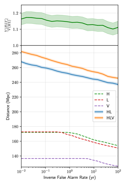
Figure 3: Sensitivity of PyCBC Live, with the O3 configuration, for a population of simulated BNS signals added to simulated Gaussian noise at design sensitivity. The “HL” configuration corresponds to a detector network formed by LIGO-Hanford and LIGO-Livingston only. The “HLV” configuration includes Virgo. The top panel shows the relative search volume of the HLV and HL configurations. The bottom panel shows sensitivity distances for the multidetector coincidence in the HL and HLV configurations (solid lines), and for the single-detector triggering (dashed lines). The lighter bands represent the $1\sigma$ uncertainties from the Monte Carlo sampling.

3.2 Sensitivity in real data

Here we repeat a similar test as presented in Subsection 3.1, with the difference that we consider broader ranges of masses and spins (therefore effectively including BBH and NSBH systems) and we add their signals to real data from the third observing run of Advanced LIGO and Advanced Virgo, as opposed to simulated stationary Gaussian detector noise. We use $\sim 8$ days of O3 data starting from 2019-05-04 13:15:32 UTC. In the simulated binaries, neutron stars have masses distributed uniformly between $1\,M_{\odot}$ and $3\,M_{\odot}$, and spin magnitudes distributed uniformly between 0 and 0.05. Black holes have masses distributed uniformly between $3\,M_{\odot}$ and $100\,M_{\odot}$, and spin magnitudes distributed uniformly between 0 and 0.985. Spins are aligned with the orbital angular momenta in all cases. BNS signals are simulated using a post-Newtonian waveform model, while NSBH and BBH signals use the SEOBNRv4_opt inspiral-merger-ringdown model (Devine et al., 2016; Bohé et al., 2017).

The resulting sensitivity for BNS mergers is shown in Figure 4. We can see that the improvement in detection rate is around 10% at false-alarm rate thresholds relevant for public alerts. This estimate is consistent with the earlier estimate from simulated data at design sensitivities. NSBH and BBH mergers, albeit arguably less interesting for rapid alerts, show similar relative improvements at the same false-alarm rate threshold, and are not shown here.

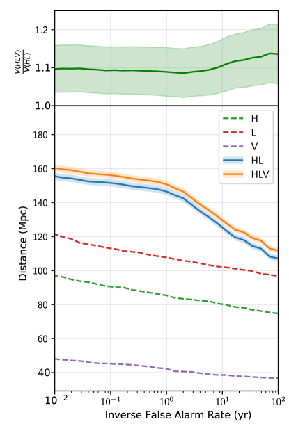
Figure 4: Comparison of PyCBC Live’s sensitivity to BNS mergers using an O2-like (“HL”) and the final-O3 (“HLV”) search configurations. The simulated signals are added to real data from Advanced LIGO and Advanced Virgo’s third run. The lighter bands represent the $1\sigma$ uncertainties from the Monte Carlo sampling.

3.3 Redetection of GW170814 and GW170817

PyCBC Live in the O3 configuration detects GW170814 in O2 data as a coincidence between the two LIGO detectors, with a LIGO-Virgo network SNR of $\approx 15$. With the method described in Section 2.3, and using 5 hours of lookback background, the candidate is assigned a false-alarm rate of 1 in $\approx 200$ yr.

The case of GW170817 is more interesting because of the glitch affecting the LIGO-Livingston data seconds before merger (Abbott et al., 2017a). Although the glitch is automatically gated by PyCBC Live, the surrounding data are still flagged as affected by a glitch by the low-latency data-quality flags, preventing a LIGO double coincidence from taking place. In addition, the small Virgo SNR also prevents a double coincidence between LIGO-Hanford and Virgo. Nevertheless, using the method described in Section 2.4, GW170817 is reported as a LIGO-Hanford single-detector candidate with false-alarm rate of 1 in $\approx 10^{9}$ yr.

PyCBC Live can also be configured to ignore data-quality flags. Under this configuration, GW170817 is detected instead as a LIGO double coincidence and is assigned a false-alarm rate lower than $1$ in $\approx 17$ yr by the method of Section 2.3. The much higher value with respect to the single-detector candidate is due to the upper limit on the double-coincident false-alarm rate imposed by the duration of the lookback background ($1$ in $100$ yr), combined with a trials factor of 6 caused by having 3 observing detectors at the time of the candidate. The absence of a detectable signal in Virgo produces a relatively large followup p-value (see Eq. 2), which cannot overcome the penalty of the trials factor. In fact, this situation matches our second numerical example in Section 2.3. Hence, when comparing these GW170817 false-alarm rates, one has to bear in mind that the LIGO-Hanford-only rate is an extrapolation from months of data, while the Hanford-Livingston-Virgo rate is an upper limit based on just $5$ hr of data.

In both configurations, however, GW170817 is reported with a false-alarm rate well beyond what is required to issue a public alert on the GCN and to consider the candidate worthwhile of followup observations.

3.4 Latency

We measure the latency of the analysis by repeatedly replaying a week of O2 data and analyzing it with PyCBC Live, thus simulating an actual observing run with a realistic computing configuration. The test amounts to a total wall-clock time of approximately $50$ days. For each candidate uploaded to GraceDB, we calculate the latency as the difference between the upload time recorded by GraceDB, and the merger time estimated by PyCBC Live. This quantity includes the processing time in PyCBC Live, as well as the latency due to the generation and distribution of the replayed O2 data. We expect the former to be the dominant contribution.

The cumulative latency distribution is shown in Figure 5. Most candidates are available in GraceDB within a few tens of seconds after coalescence, as expected. The tail extending to $\approx 100$ s is due to occasional and temporary issues with the computing infrastructure running the test, typically starvation of the available computational resources or interruptions of network connections. A similar tail is also found in a typical production analysis.

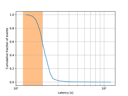
Figure 5: Cumulative distribution of PyCBC Live’s latency, for a period of replayed O2 data analyzed using the O3 configuration. The latency is defined here as the time elapsed between the estimated coalescence time of a candidate and the time of creation of the corresponding GraceDB event. The shaded region is the range of expected latency due to PyCBC Live alone, as described in Nitz et al. (2018).

3.5 Astrophysical classification

In order to test the chirp-mass-based classification of Section 2.5 we used the same population of simulated signals described in Section 3.2, with an additional constraint. Given the $1\,M_{\odot}<m<45\,M_{\odot}$ limits imposed on component masses, the results for asymmetric high-mass NSBH systems outside these limits are not representative of its accuracy of the method: here, we restrict the black hole components of simulated NSBH events to be below $50\,M_{\odot}$. For each simulation recovered by the search, we find the estimated source probabilities $\left\{P_{\rm BNS},P_{\rm NSBH},P_{\rm MG},P_{\rm BBH}\right\}$. We then consider the figures of merit shown in Figure 6.

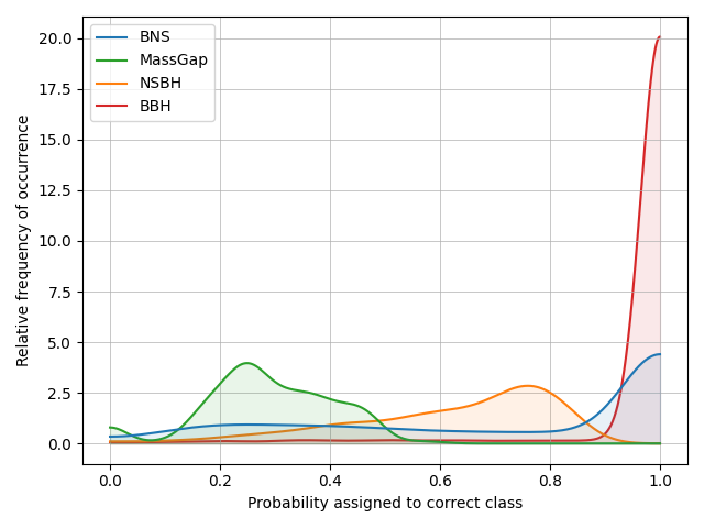
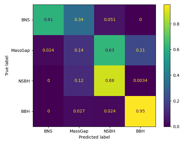
Figure 6: Left: For simulated signals of each source type, we show the probability density distribution of assigned probabilities for the recovered event to be of the same (i.e. correct) type. Right: Confusion matrix for the source classification assigned the highest probability for each simulated signal.

The first figure of merit is the distribution of probabilities for correct classification, plotted for each category as determined by the true source masses. The great majority of BNS and BBH simulations are assigned high or very high correct class probabilities, as expected given the positions of the target classes in the $m_{1}$–$m_{2}$ plane. No NSBH simulations are assigned very high probabilities of NSBH origin, since their contours of constant chirp mass always overlap other source target regions to some extent, but the majority are assigned $P_{\rm NSBH}>0.5$. In contrast, the majority of MassGap simulations are assigned $P_{\rm MG}\lesssim 0.5$; this again is expected due to the narrow extent of the MassGap region and its very high overlap with other source target regions.

The second figure of merit is the correctness of the highest estimated probability for each simulation, i.e. the most likely source category as assigned by our method. Comparing this highest probability to the true (target) classification determined by the simulated source masses, we construct the confusion matrix shown in the right panel of Figure 6. Simulations of all source types except MassGap are assigned most likely classifications that are correct in a large majority of cases; MassGap simulations are, though, preferentially assigned as most likely to be NSBH. Given the very high uncertainties on the rates and masses of actual NSBH and MassGap sources (e.g. Abbott et al. 2020c), this bias can be argued to be acceptable, and will also yield a conservative outcome as the method will err on the side of recommending EM followup for signals consistent with NSBH origin even if the true source class is MassGap.

4 Discussion

We described how the PyCBC Live analysis was improved with respect to the O2 configuration between the end of O2 and the end of O3. The most significant changes are the inclusion of more than two detectors in the significance calculation, which allowed Virgo to play a prominent role in the generation of O3 candidates, and the ability to assign significances based on data from a single detector. The single-detector significance calculation and source classification methods were not used during O3 due to its premature end, but they are ready to be utilised in future runs. We evaluated these improvements in multiple ways: first by recovering simulated signals added into ideal detector noise, then by recovering simulated signals added into real O3 data, and finally by reanalyzing a segment of O2 data containing the GW170814 and GW170817 events, and discussing how these events are detected by the new analysis. The improvements we introduced do not impact the latency.

During O3, $56$ alerts were issued on the GCN without retraction. PyCBC Live contributed to $34$ of them. Only $1$ of the $24$ retracted alerts was produced by PyCBC Live.

The next observing run will include a brand new detector, KAGRA. Unless Virgo and KAGRA reach a sensitivity comparable to LIGO, the larger resulting detector network will probably warrant further development of the multidetector significance calculation in order to limit the impact of trials factors, as discussed earlier.

In preparation for the next observing run, we plan to investigate further improvements in the handling of instrumental transients. In particular, the inpainting method presented by Zackay et al. (2021b) could potentially broaden the applicability of gating to a wider class of glitches, if it is compatible with the latency requirements of PyCBC Live. We also plan to study the impact of applying data-quality flags to the online analysis, and to characterize the effect of the SNR maximization implemented during O3.

Our proposed rapid source classification method could also be extended to consider template parameters other than the chirp mass, although these are subject to higher statistical and systematic errors (e.g. Biscoveanu et al., 2019). A possible implementation using a larger set of triggers associated with a given astrophysical event to quantify parameter errors was shown in Stachie et al. (2021).

Finally, as the latency of the entire LIGO-Virgo public alert system keeps being reduced, further development is also under way to reduce the latency of PyCBC Live. In particular, the so-called “early-warning” detection of BNS mergers (Cannon et al., 2012; Sachdev et al., 2020; Magee et al., 2021) has been implemented in PyCBC Live as well (Nitz et al., 2020c), and will be optimized and characterized in a future study.

References

- Aasi et al. (2015) Aasi, J., et al. 2015, Class. Quant. Grav., 32, 074001, doi: 10.1088/0264-9381/32/7/074001
- Abbott et al. (2016) Abbott, B., et al. 2016, Phys. Rev. D, 93, 122003, doi: 10.1103/PhysRevD.93.122003
- Abbott et al. (2017a) —. 2017a, Phys. Rev. Lett., 119, 161101, doi: 10.1103/PhysRevLett.119.161101
- Abbott et al. (2019a) —. 2019a, Phys. Rev. X, 9, 031040, doi: 10.1103/PhysRevX.9.031040
- Abbott et al. (2020a) —. 2020a, Astrophys. J. Lett., 892, L3, doi: 10.3847/2041-8213/ab75f5
- Abbott et al. (2017b) Abbott, B. P., et al. 2017b, Astrophys. J., 848, L13, doi: 10.3847/2041-8213/aa920c
- Abbott et al. (2017c) —. 2017c, Astrophys. J., 848, L12, doi: 10.3847/2041-8213/aa91c9
- Abbott et al. (2017d) —. 2017d, Phys. Rev. Lett., 118, 221101, doi: 10.1103/PhysRevLett.118.221101
- Abbott et al. (2017e) —. 2017e, The Astrophysical Journal, 851, L35, doi: 10.3847/2041-8213/aa9f0c
- Abbott et al. (2017f) —. 2017f, Phys. Rev. Lett., 119, 141101, doi: 10.1103/PhysRevLett.119.141101
- Abbott et al. (2018) —. 2018, Living Rev. Rel., 21, 3, doi: 10.1007/s41114-018-0012-9, 10.1007/lrr-2016-1
- Abbott et al. (2019b) —. 2019b, Astrophys. J. Lett., 882, L24, doi: 10.3847/2041-8213/ab3800
- Abbott et al. (2020b) Abbott, R., et al. 2020b, Phys. Rev. D, 102, 043015, doi: 10.1103/PhysRevD.102.043015
- Abbott et al. (2020c) —. 2020c, The Astrophysical Journal, 896, L44, doi: 10.3847/2041-8213/ab960f
- Abbott et al. (2020d) —. 2020d, Phys. Rev. Lett., 125, 101102, doi: 10.1103/PhysRevLett.125.101102
- Abbott et al. (2021a) —. 2021a, Phys. Rev. X, 11, 021053, doi: 10.1103/PhysRevX.11.021053
- Abbott et al. (2021b) —. 2021b, Astrophys. J. Lett., 913, L7, doi: 10.3847/2041-8213/abe949
- Acernese et al. (2015) Acernese, F., et al. 2015, Class. Quant. Grav., 32, 024001, doi: 10.1088/0264-9381/32/2/024001
- Adams et al. (2016) Adams, T., Buskulic, D., Germain, V., et al. 2016, Class. Quant. Grav., 33, 175012, doi: 10.1088/0264-9381/33/17/175012
- Akutsu et al. (2020) Akutsu, T., Ando, M., Arai, K., et al. 2020, Progress of Theoretical and Experimental Physics, 2021, doi: 10.1093/ptep/ptaa125
- Allen (2005) Allen, B. 2005, Phys. Rev. D, 71, 062001, doi: 10.1103/PhysRevD.71.062001
- Allen et al. (2012) Allen, B., Anderson, W. G., Brady, P. R., Brown, D. A., & Creighton, J. D. E. 2012, Phys. Rev. D, 85, 122006, doi: 10.1103/PhysRevD.85.122006
- Aso et al. (2013) Aso, Y., Michimura, Y., Somiya, K., et al. 2013, Phys. Rev. D, 88, 043007, doi: 10.1103/PhysRevD.88.043007
- Aubin et al. (2021) Aubin, F., et al. 2021, Class. Quant. Grav., 38, 095004, doi: 10.1088/1361-6382/abe913
- Babak et al. (2013) Babak, S., et al. 2013, Phys. Rev. D, 87, 024033, doi: 10.1103/PhysRevD.87.024033
- Biscoveanu et al. (2019) Biscoveanu, S., Vitale, S., & Haster, C.-J. 2019, Astrophys. J. Lett., 884, L32, doi: 10.3847/2041-8213/ab479e
- Bohé et al. (2013) Bohé, A., Marsat, S., & Blanchet, L. 2013, Class. Quant. Grav., 30, 135009, doi: 10.1088/0264-9381/30/13/135009
- Bohé et al. (2017) Bohé, A., Shao, L., Taracchini, A., et al. 2017, Phys. Rev. D, 95, 044028, doi: 10.1103/PhysRevD.95.044028
- Buonanno et al. (2009) Buonanno, A., Iyer, B., Ochsner, E., Pan, Y., & Sathyaprakash, B. 2009, Phys. Rev. D, 80, 084043, doi: 10.1103/PhysRevD.80.084043
- Callister et al. (2017) Callister, T., Kanner, J., Massinger, T., Dhurandhar, S., & Weinstein, A. 2017, Class. Quant. Grav., 34, 155007, doi: 10.1088/1361-6382/aa7a76
- Cannon et al. (2012) Cannon, K., et al. 2012, Astrophys. J., 748, 136, doi: 10.1088/0004-637X/748/2/136
- Chatterjee et al. (2020) Chatterjee, D., Ghosh, S., Brady, P. R., et al. 2020, Astrophys. J., 896, 54, doi: 10.3847/1538-4357/ab8dbe
- Chu (2017) Chu, Q. 2017, PhD thesis, The University of Western Australia
- Chu et al. (2020) Chu, Q., et al. 2020. https://arxiv.org/abs/2011.06787
- Dal Canton et al. (2014) Dal Canton, T., Bhagwat, S., Dhurandhar, S., & Lundgren, A. 2014, Class. Quant. Grav., 31, 015016, doi: 10.1088/0264-9381/31/1/015016
- Dal Canton & Harry (2017) Dal Canton, T., & Harry, I. W. 2017. https://arxiv.org/abs/1705.01845
- Davies et al. (2020) Davies, G. S., Dent, T., Tápai, M., et al. 2020, Phys. Rev. D, 102, 022004, doi: 10.1103/PhysRevD.102.022004
- Davis et al. (2021) Davis, D., et al. 2021, Class. Quant. Grav., 38, 135014, doi: 10.1088/1361-6382/abfd85
- Devine et al. (2016) Devine, C., Etienne, Z. B., & McWilliams, S. T. 2016, Class. Quant. Grav., 33, 125025, doi: 10.1088/0264-9381/33/12/125025
- Fisher (1970) Fisher, R. A. 1970, Statistical methods for research workers, 14th edn. (Edinburgh: Oliver and Boyd)
- Foucart et al. (2018) Foucart, F., Hinderer, T., & Nissanke, S. 2018, Physical Review D, 98, doi: 10.1103/physrevd.98.081501
- Hooper et al. (2012) Hooper, S., Chung, S. K., Luan, J., et al. 2012, Phys. Rev. D, 86, 024012, doi: 10.1103/PhysRevD.86.024012
- Iyer et al. (2011) Iyer, B., et al. 2011, LIGO-India. https://dcc.ligo.org/ligo-M1100296/public
- Kapadia et al. (2020) Kapadia, S. J., et al. 2020, Class. Quant. Grav., 37, 045007, doi: 10.1088/1361-6382/ab5f2d
- Klimenko et al. (2016) Klimenko, S., et al. 2016, Phys. Rev. D, 93, 042004, doi: 10.1103/PhysRevD.93.042004
- LIGO Scientific and Virgo Collaborations (2019) LIGO Scientific and Virgo Collaborations. 2019, Public Alerts User Guide, https://emfollow.docs.ligo.org/userguide/. https://emfollow.docs.ligo.org/userguide/
- Magee et al. (2021) Magee, R., et al. 2021, Astrophys. J. Lett., 910, L21, doi: 10.3847/2041-8213/abed54
- Messick et al. (2017) Messick, C., et al. 2017, Phys. Rev., D95, 042001, doi: 10.1103/PhysRevD.95.042001
- Nitz et al. (2020a) Nitz, A., Harry, I., Brown, D., et al. 2020a, gwastro/pycbc: PyCBC, Zenodo, doi: 10.5281/zenodo.596388
- Nitz (2018) Nitz, A. H. 2018, Class. Quant. Grav., 35, 035016, doi: 10.1088/1361-6382/aaa13d
- Nitz et al. (2019a) Nitz, A. H., Capano, C., Nielsen, A. B., et al. 2019a, Astrophys. J., 872, 195, doi: 10.3847/1538-4357/ab0108
- Nitz et al. (2021) Nitz, A. H., Capano, C. D., Kumar, S., et al. 2021. https://arxiv.org/abs/2105.09151
- Nitz et al. (2018) Nitz, A. H., Dal Canton, T., Davis, D., & Reyes, S. 2018, Phys. Rev., D98, 024050, doi: 10.1103/PhysRevD.98.024050
- Nitz et al. (2017) Nitz, A. H., Dent, T., Dal Canton, T., Fairhurst, S., & Brown, D. A. 2017, Astrophys. J., 849, 118, doi: 10.3847/1538-4357/aa8f50
- Nitz et al. (2020b) Nitz, A. H., Dent, T., Davies, G. S., & Harry, I. 2020b, Astrophys. J., 897, 2, doi: 10.3847/1538-4357/ab96c7
- Nitz et al. (2020c) Nitz, A. H., Schäfer, M., & Dal Canton, T. 2020c, Astrophys. J. Lett., 902, L29, doi: 10.3847/2041-8213/abbc10
- Nitz et al. (2019b) Nitz, A. H., Dent, T., Davies, G. S., et al. 2019b, Astrophys. J., 891, 123, doi: 10.3847/1538-4357/ab733f
- Pürrer (2014) Pürrer, M. 2014, Class. Quant. Grav., 31, 195010, doi: 10.1088/0264-9381/31/19/195010
- Roy et al. (2018) Roy, S., Sankar Sengupta, A., & Ajith, P. 2018, in 42nd COSPAR Scientific Assembly, Vol. 42, E1.15–36–18
- Roy et al. (2019) Roy, S., Sengupta, A. S., & Ajith, P. 2019, Phys. Rev. D, 99, 024048, doi: 10.1103/PhysRevD.99.024048
- Roy et al. (2017) Roy, S., Sengupta, A. S., & Thakor, N. 2017, Phys. Rev. D, 95, 104045, doi: 10.1103/PhysRevD.95.104045
- Sachdev et al. (2019) Sachdev, S., et al. 2019. https://arxiv.org/abs/1901.08580
- Sachdev et al. (2020) —. 2020, Astrophys. J. Lett., 905, L25, doi: 10.3847/2041-8213/abc753
- Singer & Price (2016) Singer, L. P., & Price, L. R. 2016, Phys. Rev. D, 93, 024013, doi: 10.1103/PhysRevD.93.024013
- Somiya (2012) Somiya, K. 2012, Class. Quant. Grav., 29, 124007, doi: 10.1088/0264-9381/29/12/124007
- Stachie et al. (2021) Stachie, C., et al. 2021, Mon. Not. Roy. Astron. Soc., 505, 4235, doi: 10.1093/mnras/stab1492
- Storn & Price (1997) Storn, R., & Price, K. 1997, Journal of Global Optimization, doi: 10.1023/A:1008202821328
- Usman et al. (2016) Usman, S. A., Nitz, A. H., Harry, I. W., et al. 2016, Class. Quant. Grav., 33, 215004, doi: 10.1088/0264-9381/33/21/215004
- Venumadhav et al. (2019) Venumadhav, T., Zackay, B., Roulet, J., Dai, L., & Zaldarriaga, M. 2019, Phys. Rev. D, 100, 023011, doi: 10.1103/PhysRevD.100.023011
- Venumadhav et al. (2020) —. 2020, Phys. Rev. D, 101, 083030, doi: 10.1103/PhysRevD.101.083030
- Zackay et al. (2021a) Zackay, B., Dai, L., Venumadhav, T., Roulet, J., & Zaldarriaga, M. 2021a, Phys. Rev. D, 104, 063030, doi: 10.1103/PhysRevD.104.063030
- Zackay et al. (2021b) Zackay, B., Venumadhav, T., Roulet, J., Dai, L., & Zaldarriaga, M. 2021b, Phys. Rev. D, 104, 063034, doi: 10.1103/PhysRevD.104.063034