Hydrodynamics of quantum entropies in Ising chains with linear dissipation

Abstract

We study the dynamics of quantum information and of quantum correlations after a quantum quench, in transverse field Ising chains subject to generic linear dissipation. As we show, in the hydrodynamic limit of long times, large system sizes, and weak dissipation, entropy-related quantities —such as the von Neumann entropy, the Rényi entropies, and the associated mutual information— admit a simple description within the so-called quasiparticle picture. Specifically, we analytically derive a hydrodynamic formula, recently conjectured for generic noninteracting systems, which allows us to demonstrate a universal feature of the dynamics of correlations in such dissipative noninteracting system. For any possible dissipation, the mutual information grows up to a time scale that is proportional to the inverse dissipation rate, and then decreases, always vanishing in the long time limit. In passing, we provide analytic formulas describing the time-dependence of arbitrary functions of the fermionic covariance matrix, in the hydrodynamic limit.

1 Introduction

Understanding the fate of entanglement and of quantum correlations in open quantum many-body systems is of paramount importance in order to assess the simulability of quantum devices with classical computers [1, 2], or to understand cold-atom experiments [3, 4, 5, 6]. However, shedding light on these aspects of dissipative many-body quantum dynamics still represents a challenging task [7].

For closed quantum many-body systems a powerful hydrodynamic picture, based on the existence of long-lived excitations, provides a thorough description of the spreading of entanglement, at least in integrable systems [8, 9, 10, 11, 12, 13, 14, 15], both free (noninteracting) and interacting ones. Unfortunately, much less is known in the presence of dissipation. Very recently, it has been shown that it is possible to extend the (hydrodynamic) quasiparticle picture in order to include the effects of dissipation in free-fermion and free-boson models [16, 17, 18] (see also Ref. [19]). In particular, building on the results discussed in Ref. [17], a formula, which allows to describe the dynamics of several entropy-related quantities, has been conjectured and thoroughly verified numerically [18] for rather general systems. However, an analytic proof of this formula is still missing, even when considering specific cases. The main contribution of this work is to analytically demonstrate the validity of the hydrodynamic picture, as described by the formula reported in Ref. [18], for the transverse field Ising chain subject to arbitrary linear dissipation.

We consider open quantum many-body dynamics of Markovian type, for which the evolution of the full system density matrix $\rho$ is given by the Lindblad equation as [20]

$$\frac{d\rho}{dt}=-i[H,\rho]+\gamma\sum_{m}\Big{(}L_{m}\rho L_{m}^{\dagger}-\frac{1}{2}\{L_{m}^{\dagger}L_{m},\rho\}\Big{)}.$$ (1)

Here, $H$ is the many-body Hamiltonian of the system, $\gamma$ represents an overall dissipation strength, and the operators $L_{m}$ encode how the presence of an environment affects the dynamics of the quantum system. We consider a bipartition of the many-body system into two complementary subsystems $A$ and $\bar{A}$, with $\bar{A}$ denoting the complement of $A$ [as illustrated in Fig. 1(a)], and study different entropy-related quantities. Namely, the Rényi entropies $S_{A}^{\scriptscriptstyle(n)}$ defined as [21, 22, 23]

$$S_{A}^{(n)}:=\frac{1}{1-n}\ln(\mathrm{Tr}\rho_{A}^{n}),\quad n\in\mathbb{R},$$ (2)

and the von Neumann entropy $S_{A}:=-\mathrm{Tr}\rho_{A}\ln(\rho_{A})$. We further consider the mutual information ${\mathcal{I}}^{\scriptscriptstyle(n)}_{A:\bar{A}}$, which is given by

$${\mathcal{I}}^{(n)}_{A:\bar{A}}:=S_{A}^{(n)}+S_{\bar{A}}^{(n)}-S_{A\cup\bar{A}}^{(n)}.$$ (3)

For a system prepared in a pure state and undergoing unitary dynamics, it is easy to show that $S_{A}^{\scriptscriptstyle(n)}=S_{\bar{A}}^{\scriptscriptstyle(n)}$ and $S_{A\cup\bar{A}}^{\scriptscriptstyle(n)}=0$. This is, however, not the case in the presence of dissipation since the total system $A\cup\bar{A}$ is, in general, in a mixed state. Furthermore, we recall here that for mixed states the Rényi entropies and the mutual information are not proper measures of quantum entanglement. In particular, the mutual information only quantifies the total (classical plus quantum) correlation between $A$ and $\bar{A}$, which bounds the quantum entanglement between them [24]. For mixed states, a proper measure of entanglement is given by the logarithmic negativity [25, 26, 27, 28, 29, 30].

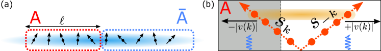
Figure 1: (a) Setup considered in this work. We focus on the quantum Ising chain subject to arbitrary linear dissipation acting on the full system. We are interested in the out-of-equilibrium dynamics of the subsystem entropies $S^{\scriptscriptstyle(n)}$ and the mutual information ${\mathcal{I}}^{\scriptscriptstyle(n)}_{A:\bar{A}}$ between a subsystem $A$ of length $\ell$ and its complement $\bar{A}$ after a generic magnetic field quench. (b) Quasiparticle (hydrodynamic) picture. Pairs of correlated quasiparticles are produced after the quench. Quasiparticles travel with opposite velocities $v(k)=v(-k)=-v(k)$, with $k$ the quasimomentum. Pairs that are shared between $A$ and $\bar{A}$ contribute with $s_{k}$ and $s_{-k}$ to the entropies. Quantum entropies also contain a contribution which is due to the system being in a mixed state [wiggly lines in (b)].

Here we consider an arbitrary magnetic field quench in an open quantum Ising chain affected by a generic linear dissipation. We rigorously show that the dynamics of the Reńyi entropy $S_{A}^{\scriptscriptstyle(n)}$ of an interval of length $\ell$ embedded in an infinite system is described by [18]

$$S_{A}^{(n)}=\int_{-\pi}^{\pi}\frac{dk}{2\pi}\Big{[}s^{(n),YY}_{k}-s^{(n),\mathrm{mix}}_{k}\Big{]}\min(\ell,2|v(k)|t)+\ell\int_{-\pi}^{\pi}\frac{dk}{2\pi}s^{(n),\mathrm{mix}}_{k}.$$ (4)

The above equation was recently conjectured in Ref. [18], and it has been verified numerically for several types of dissipation. Eq. (4) holds in what we call here the weakly-dissipative hydrodynamic limit characterized by $\ell,t\to\infty$, $\gamma\to 0$ with $\ell/t$ and $\gamma\ell$ fixed, where $\gamma$ is the overall dissipation strength [see Eq. (1)] and $\ell$ is the size of the subsystem $A$ [cf. Fig. 1]. The first term in (4) describes the spreading of correlations due to correlated pairs of quasiparticles traveling with velocities $v(k)$ and $v(-k)$. This term is similar to the one appearing in the unitary case, i.e., without dissipation. Remarkably, as we discuss, the group velocities $v(k)$ of the quasiparticles are not affected by the dissipation, and this could be attributed to the fact that the dissipation is linear and weak. The term $s^{\scriptscriptstyle(n),YY}_{k}$ in the square brackets is reminiscent of the Yang-Yang entropy in the unitary case [31]. The term $s_{k}^{\scriptscriptstyle(n),\mathrm{mix}}$ is purely dissipative. Indeed, for $\gamma=0$ and starting from a pure state, one has that $s_{k}^{\scriptscriptstyle(n),\mathrm{mix}}=0$, and $s_{k}^{\scriptscriptstyle(n),YY}$ becomes the Yang-Yang entropy. In contrast with the unitary case, in the presence of dissipation both $s_{k}^{\scriptscriptstyle(n),YY}$ and $s_{k}^{\scriptscriptstyle(n),\mathrm{mix}}$ are time-dependent. As it is clear from (4), the effect of $s_{k}^{\scriptscriptstyle(n),\mathrm{mix}}$ is twofold. Specifically, it gives a volume-law contribution associated with the mixedness of the quantum state [see second term in (4)], and it reduces the total correlation between the quasiparticle pairs (term with the minus sign in (4)). Interestingly, in the limit $t\to\infty$ the term in the square brackets vanishes for any type of dissipation. We also provide a formula for the mutual information, which, in agreement with the result of Ref. [17] and [18], depends only on the first term in (4). Surprisingly, while for most of the dissipators the Yang-Yang term $s_{k}^{\scriptscriptstyle(n),YY}$ is determined by the dynamics of the density of quasiparticles that diagonalize the Ising chain, this is not true in general. We also show that, for those dissipations for which this is not true, $s_{k}^{\scriptscriptstyle(n),YY}$ is not an even function of $k$, in stark contrast with the usually considered Hamiltonian cases, and with the dissipators of Ref. [18]. Finally, as a byproduct of our analysis we provide exact formulas describing the weakly-dissipative hydrodynamic limit of arbitrary functions of the fermionic covariance matrix of the Ising chain, generalizing the result of Ref. [32] to dissipative settings.

The manuscript is organized as follows. In section 2 we introduce the quantum Ising chain (see section 2.1), the quench protocol (section 2.2), and the Lindblad framework that we exploit to account for dissipation 2.3. In section 3 we derive the behavior of the fermionic covariance matrix in the weakly-dissipative hydrodynamic limit. In section 4 we present our main results, which are formulae (60) (63), and (68). Section 4.1 is devoted to the dynamics of the density of the quasiparticles, whereas in section (4.2) we discuss the steady-state value of the subsystem entropies. In section 5 we provide numerical results. Specifically, we discuss numerical benchmarks for the entropy and the mutual information in section 5.1, section 5.2, and section 5.3. Finally, we present our conclusions in section 6. In A we review the calculation of subsystem entropies for free-fermion systems. In B and C we report a complete derivation of the results of section 4.

2 Model, quench, and dissipation

In this paper, we are interested in the interplay between out-of-equilibrium unitary dynamics after a quantum quench [33, 34, 35, 36] in the quantum Ising chain and the presence of arbitrary linear dissipation. In this section, we start by reviewing some relevant aspects of the Ising chain and then discuss the quantum quench protocol (magnetic field quench). Finally, in section 2.3 we introduce the Lindblad framework for Markovian open quantum dynamics.

2.1 Ising (Kitaev) chain

We consider the quadratic fermionic chain defined by the Hamiltonian

$$H=-J\sum_{j=1}^{L}(c^{\dagger}_{j}c_{j+1}+c^{\dagger}_{j+1}c_{j}-\delta c_{j}c_{j+1}-\delta c^{\dagger}_{j+1}c^{\dagger}_{j}-2hc^{\dagger}_{j}c_{j})-JhL.$$ (5)

Here $c_{j}$ are standard fermionic operators acting on site $j$ of the chain, and $L$ is the length of the chain. We use periodic boundary conditions $c_{j+L}=c_{j}$. In (5) $h$ is the external magnetic field, and $J,\delta$ real parameters. In the following we are going to fix $\delta=1$, although our results could be extended to arbitrary $\delta$. We also fix $J=1$. The Hamiltonian (5) is obtained from the transverse field Ising chain after a Jordan-Wigner transformation [37]. The total number of fermions $\hat{N}:=\sum_{j}c^{\dagger}_{j}c_{j}$ is not conserved for $\delta\neq 0$, whereas the fermion parity $e^{i\pi\hat{N}}$ is a conserved quantitiy. Importantly, the Jordan-Wigner transformation is crucial in order to extract physical quantities both at equilibrium and out-of-equilibrium in the transverse field Ising chain. For instance, the Jordan-Wigner string affects the boundary conditions that have to be imposed on the fermions. Specifically, periodic boundary conditions on the spins are mapped to periodic or antiperiodic ones for the fermions, depending on the parity of the fermion number. Here, however, to avoid all these complications we work directly with the fermionic Hamiltonian (5) with periodic boundary conditions.

It is convenient to rewrite (5) in terms of Majorana fermions. Let us define two species of Majorana operators $w_{1,j}$ and $w_{2,j}$ as

$$w_{1,j}=c^{\dagger}_{j}+c_{j},\quad w_{2,j}=i(c_{j}-c^{\dagger}_{j}),$$ (6)

with standard anticommutation relations

$$\{w_{s,j},w_{s^{\prime},j^{\prime}}\}=2\delta_{j,j^{\prime}}\delta_{s,s^{\prime}}.$$ (7)

It is convenient to think of these operators as the elements of a $2L$-dimensional operator-valued vector defined as $w_{2j-1}:=w_{1,j}$ and $w_{2j}:=w_{2,j}$. We will exploit this formalism when introducing the dissipative contribution to the dynamics below. By using (6), the Hamiltonian (5) is recast as

$$H=\sum_{j,m=1}^{L}(w_{1,j},\,w_{2,j})h_{j,m}\left(\begin{array}[]{c}w_{1,m}\\ w_{2,m}\end{array}\right).$$ (8)

Here $h_{j,m}$ is the following $2\times 2$ matrix

$$h_{j,m}=\frac{i}{2}\left(\begin{array}[]{cc}0&\delta_{j,m+1}-h\delta_{j,m}\\ -\delta_{j,m-1}+h\delta_{j,m}&0\end{array}\right),$$ (9)

specifying the (quadratic) interaction between site $j$ and site $m$. By exploiting translation invariance, Eq. (9) can be rewritten as

$$h_{j,m}=\int_{-\pi}^{\pi}\frac{dk}{2\pi}e^{-i(j-m)k}\hat{h}_{k},$$ (10)

where we introduce the so-called symbol $\hat{h}_{k}$ of the Hamiltonian

$$\hat{h}_{k}=\frac{i}{2}\left(\begin{array}[]{cc}0&e^{ik}-h\\ -e^{-ik}+h&0\end{array}\right).$$ (11)

The fermionic Ising chain is diagonalized in terms of Bogoliubov modes $\alpha_{k}$. After a Bogoliubov transformation, indeed, Eq. (8) becomes

$$H=\sum_{k}\varepsilon_{h}(k)\alpha^{\dagger}_{k}\alpha_{k}.$$ (12)

Here $\alpha_{k}$ satisfy standard fermionic anticommutation relations, and $\varepsilon_{h}(k)$ is the single-particle dispersion relation

$$\varepsilon_{h}(k)=2J\sqrt{1+h^{2}-2h\cos(k)}.$$ (13)

The Bogoliubov fermions $\alpha_{k}$ are defined in terms of the Fourier transforms of original fermions $c_{k}$ and $c^{\dagger}_{-k}$ as

$$(\alpha_{k},\alpha_{-k}^{\dagger})=\left(\begin{array}[]{cc}\cos(\frac{\theta_{k}}{2})&i\sin(\frac{\theta_{k}}{2})\\ i\sin(\frac{\theta_{k}}{2})&\cos(\frac{\theta_{k}}{2})\end{array}\right)\left(\begin{array}[]{c}c_{k}\\ c^{\dagger}_{-k}\end{array}\right)$$ (14)

where $c_{k}:=L^{-1/2}\sum_{j=1}^{L}e^{ikj}c_{j}$. In (14), we introduced the Bogoliubov angle $\theta_{k}$ defined through the relation

$$e^{i\theta_{k}}=\frac{h-e^{ik}}{\sqrt{1+h^{2}-2h\cos(k)}}.$$ (15)

A crucial ingredient for the following is the Majorana covariance matrix $\Gamma$. This is defined through the $2\times 2$ blocks

$$\Gamma_{j,j^{\prime}}=\left(\begin{array}[]{cc}\langle w_{1,j}w_{1,j^{\prime}}\rangle-\delta_{j,j^{\prime}}&\langle w_{1,j}w_{2,j^{\prime}}\rangle\\ \langle w_{2,j}w_{1,j^{\prime}}\rangle&\langle w_{2,j}w_{2,j^{\prime}}\rangle-\delta_{j,j^{\prime}}\end{array}\right),\quad j,j^{\prime}=1,\dots,L,$$ (16)

where $\langle x\rangle:=\mathrm{Tr}(\rho x)$, and $\rho$ is the density matrix that describes the state of the system. In translational invariant situations, $\Gamma$ depends only on $j-j^{\prime}$ and it can be written in terms of its symbol $\hat{\Gamma}_{k}$ as

$$\Gamma_{j,j^{\prime}}(t)=\int_{-\pi}^{\pi}\frac{dk}{2\pi}e^{-ik(j-j^{\prime})}\hat{\Gamma}_{k}(t).$$ (17)

It is well-known [38] that from (16) it is possible to extract the von Neumann entropy and the Rényi entropies of a subsystem $A$ (see A).

2.2 Magnetic field quench

The protocol of the magnetic field quench is as follows: At $t=0$ the chain is prepared in the ground state of (5) at $h_{0}$. Then the magnetic field is suddenly changed to its final value $h_{0}\to h$. Since the initial state is not an eigenstate of the final Hamiltonian, in the absence of dissipation, the chain undergoes nontrivial unitary dynamics. The generic magnetic field quench is parametrized in terms of a new Bogoliubov angle [32, 39, 40] $\Delta_{k}$. This is given as $\Delta_{k}:=\theta_{k}-\theta_{k}^{0}$, where $\theta_{k}$ is defined in (15) and $\theta_{k}^{0}$ is obtained from (15) by setting $h\to h_{0}$. The angle $\Delta_{k}$ enters in the transformation between the Bogoliubov modes $\alpha_{k}$ and $\alpha_{k}^{0}$ diagonalizing the Ising Hamiltonian with magnetic field $h$ and $h_{0}$, respectively. Both modes $\alpha_{k}$ and $\alpha_{k}^{0}$ are written in terms of the same fermions $c_{k}$, implying that the angle $\Delta_{k}$ is easily obtained from (14). Specifically, one obtains that

$$\cos(\Delta_{k})=4\frac{1+h_{0}h+\cos(k)(h+h_{0})}{\varepsilon_{h_{0}}(k)\varepsilon_{h}(k)}$$ (18)

$$\sin(\Delta_{k})=4\frac{\sin(k)(h_{0}-h)}{\varepsilon_{h}(k)\varepsilon_{h_{0}}(k)}.$$ (19)

Here $\varepsilon_{h}$ is the dispersion of the Bogoliubov quasiparticles (cf. (13)).

We are interested in the dynamics of the covariance matrix $\Gamma$ (cf. (16)). First, the ground-state pre-quench matrix $\Gamma(0)$ can be derived explicitly [39]. The associated symbol $\hat{\Gamma}_{k}$ reads as

$$\hat{\Gamma}_{k}(0)=-i\left(\begin{array}[]{cc}0&-e^{i\theta_{k}+i\Delta_{k}}\\ e^{-i\theta_{k}-i\Delta_{k}}&0\end{array}\right),$$ (20)

where $\Delta_{k}$ and $\theta_{k}$ are defined in (18) (19) and (15). The evolved symbol $\Gamma_{k}(t)$ is obtained from (20) as

$$\hat{\Gamma}_{k}(t)=\hat{U}_{k}\hat{\Gamma}_{k}(0)\hat{U}_{-k}^{T}.$$ (21)

Here $T$ denotes matrix transposition, and the symbol of the evolution operator $\hat{U}_{k}$ is given as

$$\hat{U}_{k}=e^{-4i\hat{h}_{k}t},$$ (22)

with $\hat{h}_{k}$ the symbol of the Hamiltonian (11). More explicitly, by using (20)(21)(22) we obtain the compact expression for $\hat{\Gamma}_{k}(t)$ as

$$\hat{\Gamma}_{k}(t)=-\cos(\Delta_{k})\sigma_{y}^{(k)}-\sin(\Delta_{k})\sigma_{x}^{(k)}e^{2i\varepsilon_{h}(k)t\sigma_{y}^{(k)}}.$$ (23)

At $t=0$ one recovers (20). Note that only the second term in (23) depends on time and that in (23) we have introduced the rotated Pauli matrices $\sigma^{(k)}_{\alpha}$ as

$$\sigma^{(k)}_{\alpha}:=e^{i\theta_{k}\sigma_{z}/2}\sigma_{\alpha}e^{-i\theta_{k}\sigma_{z}/2},\quad\alpha=x,y,z,$$ (24)

where $\sigma_{\alpha}$ with $\alpha=x,y,z$ are the standard Pauli matrices. The definition (24) will be convenient in section 3 to derive the dynamics of $\hat{\Gamma}_{k}(t)$ in the presence of dissipation. To obtain (23) we used the commutation relations of the Pauli matrices and that $[\sigma_{y}^{\scriptscriptstyle(-k)}]^{T}=-\sigma_{y}^{\scriptscriptstyle(k)}$.

The Majorana covariance matrix $\Gamma$ is obtained as the inverse Fourier transform of (23) as

$$\Gamma=-i\left(\begin{array}[]{cc}f_{j-j^{\prime}}(t)&-g_{-(j-j^{\prime})}(t)\\ g_{j-j^{\prime}}(t)&-f_{j-j^{\prime}}(t)\end{array}\right),$$ (25)

where we defined the functions $f_{j-j^{\prime}}$ and $g_{j-j^{\prime}}$ as

$$f_{l}(t) =i\int_{-\pi}^{\pi}\frac{dk}{2\pi}e^{-ikl}\sin(\Delta_{k})\sin(2\varepsilon_{h}(k)t),$$ (26)

$$g_{l}(t) =-\int_{-\pi}^{\pi}\frac{dk}{2\pi}e^{-ikl}e^{-i\theta_{k}}\Big{[}\cos(\Delta_{k})-i\sin\Delta_{k}\cos(2\varepsilon_{h}(k)t)\Big{]}.$$ (27)

In this work we focus on the thermodynamic limit and on the long-time limit after the quench. In this limit, the reduced-density matrix of any finite subystem $A$ (see Fig. 1) reaches a steady state that is described by a Generalized Gibbs Ensemble (GGE) [34, 36, 35]. The GGE is identified by the occupations (densities) $\rho_{k}$ of the modes $\alpha_{k}$ (cf. (12)). These are obtained as the expectation value

$$\rho_{k}:=\langle h_{0}|\alpha^{\dagger}_{k}\alpha_{k}|h_{0}\rangle,$$ (28)

where $|h_{0}\rangle$ is the pre-quench initial state. The density $\rho_{k}$ is preserved during the unitary dynamics after the quench. Crucially, this is not the case in the presence of dissipation. We will derive the dynamics of $\rho_{k}$ in the presence of dissipation in section 3. By using the explicit form of the operators $\alpha_{k}$ one obtains that [32]

$$\rho_{k}=\frac{1-\cos(\Delta_{k})}{2}.$$ (29)

It is useful to stress that by using (14) it is possible to express the Bogoliubov modes $\alpha_{k}$ in terms of Majorana operators $w_{s,j}$ (cf. (6)), which allows to rewrite $\rho_{k}$ in terms of the matrix elements of $\hat{\Gamma}_{k}$. The result reads as [40]

$$\rho_{k}=\frac{1}{2}(1-\mathrm{Im}(e^{-i\theta_{k}}[\hat{\Gamma}_{k}]_{12})),$$ (30)

where $[\hat{\Gamma}_{k}]_{12}$ is the only independent off-diagonal entry of $\hat{\Gamma}_{k}(t)$ (cf. (21)). In the presence of dissipation Eq. (30) provides a way to extract how the density of modes $\alpha_{k}$ evolves under the combined action of unitary and dissipative terms.

2.3 Lindblad evolution of the covariance matrix

Here we consider a generic Liovillian dynamics (see (1)) for the Ising chain (5) subject to arbitrary one-site translation invariant linear Lindblad operators. This type of dissipation can be treated within the framework of the so-called third quantization [41]. Instead of considering the dynamics of the system density matrix (1), it is convenient to focus on a generic observables $X_{t}$. Eq. (1) can be recast in the convenient form

$$\frac{dX_{t}}{dt}=i[H,X_{t}]+\sum_{m,j=1}^{2L}K_{mj}\left(w_{m}X_{t}w_{j}-\frac{1}{2}\left\{X_{t},w_{m}w_{j}\right\}\right),$$ (31)

where $w_{j}$ are Majorana operators, $H$ is the system Hamiltonian written in the Majorana basis. Eq. (31) is written in terms of the $2L$ Majorana fermions $w_{2j-1}:=w_{1,j}$ and $w_{2j}:=w_{2,j}$ (cf. (6)). In (31) the dissipation is encoded in the so-called Kossakowski matrix [42, 43] $K_{mj}$. We make here a remark about the notation of the paper. With the writing $K_{mj}$, as in the above equation, we indicate the element of the $2L\times 2L$ matrix $K$ in the $m$th row and $j$th column. With the writing $K_{m,j}$, for instance appearing in Eq. (10) for $h$, instead, we denote the $2\times 2$ block of $K$ in the $m,j$ position.

Importantly, since the evolution implemented by Eq. (31) has to be completely positive (see [20]), the Kossakowski matrix $K_{mj}$ has to be positive semi-definite [43]. For later convenience, we can decompose $K$ as

$$K^{\mathrm{Re}}:=\frac{1}{2}(K+K^{*})=(K^{\mathrm{Re}})^{T}$$ (32)

$$K^{\mathrm{Im}}:=\frac{1}{2i}(K-K^{*})=-(K^{\mathrm{Im}})^{T},$$ (33)

where we suppressed the indices in $K_{mj}$ to lighten the notation. The superscripts $\mathrm{Re}$ and $\mathrm{Im}$ denote the real and imaginary parts of $K$, respectively. Again, for translation invariant dissipation, by going to momentum space, one defines the symbol $\hat{K}_{k}$ of $K$ through the relation

$$K_{m,j}=\int_{-\pi}^{\pi}\frac{dk}{2\pi}e^{-ik(m-j)}\hat{K}_{k},$$ (34)

where we remark one more time that $K_{m,j}$ is a $2\times 2$ block of $K$. We note that for the positivity of $K$, one has that $\hat{K}_{k}$ has to be positive. Using Eq. (31) on products of Majorana operators in order to find the dynamics of $\Gamma$, one gets the differential equation [18]

$$\frac{d}{dt}\Gamma=\Lambda\Gamma+\Gamma\Lambda^{T}+4iK^{\mathrm{Im}}.$$ (35)

Here we defined the matrix $\Lambda$ to be

$$\Lambda:=-4ih-2K^{\mathrm{Re}},$$ (36)

with $h$ the Hamiltonian matrix in the basis of Majorana defined in (9). Interestingly, as it is clear from (35), only the real part $K^{\mathrm{Re}}$ enters in the matrix $\Lambda$, whereas $K^{\mathrm{Im}}$ acts as a driving term. Eq. (35) has the formal solution

$$\Gamma(t)=\widetilde{U}(t)\Gamma(0)\widetilde{U}^{T}(t)+4i\int_{0}^{t}du\,\widetilde{U}(t-u)K^{\mathrm{Im}}\widetilde{U}^{T}(t-u)\,,$$ (37)

where the evolution operator $\widetilde{U}(t)$ is defined as $\widetilde{U}(t):=e^{\Lambda t}$. For translation invariant systems, Eq. (37) can be recast as an equation for the symbol $\hat{\Gamma}_{k}$ (cf. (17)). Specifically, one obtains that

$$\hat{\Gamma}_{k}(t)={\widetilde{U}}_{k}\hat{\Gamma}_{k}(0)\widetilde{U}^{T}_{-k}(t)+4i\int_{0}^{t}du\widetilde{U}_{k}(t-u)\hat{K}_{k}^{\mathrm{Im}}\widetilde{U}^{T}_{-k}(t-u).$$ (38)

Here $\hat{\Gamma}_{k},\hat{\Lambda}_{k},\hat{K}_{k}^{\mathrm{Im}}$ are the symbols of the matrices $\Gamma,\Lambda,K^{\mathrm{Im}}$, and are $2\times 2$ matrices. The integral in Eq. (38) can be performed explicitly, although for generic dissipation the result is quite cumbersome. Still, Eq. (38) is useful to obtain exact numerical results for $\hat{\Gamma}_{k}$. Further simplifications occur in the hydrodynamic limit $t\to\infty$ with weak dissipation, as we are going to show.

To proceed, let us consider the most general Kossakowski matrix $K$. Since its symbol $\hat{K}_{k}$ has to be hermitian (actually positive), it has to be of the form

$$\hat{K}_{k}=\gamma\left(\begin{array}[]{cc}a(k)&c(k)\\ c^{*}(k)&b(k)\end{array}\right).$$ (39)

In (39) we re-introduced the strength of the dissipation $\gamma$. The weak-dissipation limit corresponds to $\gamma\to 0$ with an appropriate scaling with $\ell$. In (39) $a(k),b(k)$ are real functions, whereas $c(k)$ is in general complex. From (39) one can obtain the symbols $\hat{K}_{k}^{\mathrm{Re}}$ and $\hat{K}_{k}^{\mathrm{Im}}$ of the real and imaginary parts of $K$ as

$$\hat{K}_{k}^{\mathrm{Re}}=\gamma\left(\begin{array}[]{cc}a_{\mathrm{e}}&c^{\mathrm{Re}}_{\mathrm{e}}+ic^{\mathrm{Im}}_{\mathrm{o}}\\ c^{\mathrm{Re}}_{\mathrm{e}}-ic^{\mathrm{Im}}_{\mathrm{o}}&b_{\mathrm{e}}\end{array}\right),\quad\hat{K}_{k}^{\mathrm{Im}}=\gamma\left(\begin{array}[]{cc}-ia_{\mathrm{o}}&-ic^{\mathrm{Re}}_{\mathrm{o}}+c^{\mathrm{Im}}_{\mathrm{e}}\\ -ic^{\mathrm{Re}}_{\mathrm{o}}-c^{\mathrm{Im}}_{\mathrm{e}}&-ib_{\mathrm{o}}\end{array}\right),$$ (40)

where $c(k)=c^{\mathrm{Re}}(k)+ic^{\mathrm{Im}}(k)$, and we introduced the odd and even functions $a_{\mathrm{e}}(k):=[a(k)+a(-k)]/2$, $a_{\mathrm{o}}:=[a(k)-a(-k)]/2$. Similar definitions hold for $b_{\mathrm{e/o}}(k)$ and $c^{\mathrm{Re/Im}}_{\mathrm{e/o}}(k)$. The decomposition (40) is obtained from (34) by using that $K^{\mathrm{Re}}=(K+K^{*})/2$ and $K^{\mathrm{Im}}=(K-K^{*})/(2i)$. We note that the fact that the symbol (39) has to be positive semi-definite for any $k$ puts some constraints on the functions $a,b,c$. Interestingly, however, the results that we derive below hold true even when $\hat{K}$ is not positive, i.e. for “unphysical” dissipation.

For the sake of concreteness, it is useful to specialize (40) to the case of gain/loss dissipation. This has been studied extensively in the literature, as it is one of the simplest yet experimentally relevant sources of dissipation [7] (see [44] for a study of the interplay between criticality and dissipation, and [45] for an application to cold-atom systems). The dynamics of the von Neumann entropy and of the mutual information in the presence of gain/loss dissipation in a simple tight-binding chain has been obtained analytically using the quasiparticle picture in Ref. [17] (see also Ref. [16] for a study in the Ising chain). The case of localized losses has been addressed in Ref. [46]. We consider gain/loss dissipation with rates $\gamma g^{\pm}$, where $\gamma$ is the strength of the dissipation, and $g^{\pm}$ real parameters. The Lindblad operators $L_{m}^{\pm}$ are given as $L_{m}^{+}=2\sqrt{\gamma g^{+}}c^{\dagger}_{m}$ and $L_{m}^{-}=2\sqrt{\gamma g^{-}}c_{m}$. These operator model the incoherent creation and loss of fermions in the chain. By using (34), one obtains that the symbol of the Kossakowski matrix $\hat{K}_{k}$ for gain/loss dissipation reads as

$$\hat{K}_{k}=\gamma\left(\begin{array}[]{cc}g^{+}+g^{-}&-i(g^{-}-g^{+})\\ +i(g^{-}-g^{+})&g^{+}+g^{-}\end{array}\right).$$ (41)

Note that $\hat{K}_{k}$ does not depend on the momentum $k$. This is a feature of dissipations which are diagonal in the lattice space. As it is clear from (41), $\hat{K}^{\mathrm{Re}}_{k}=(g^{+}+g^{-})\mathds{1}_{2}$, where $\mathds{1}_{2}$ is the $2\times 2$ identity matrix. This implies that the dynamics is determined by the model without dissipation (cf. (36)), apart from an exponential damping factor $e^{-2\gamma(g^{+}+g^{-})t}$. The driving term (cf. (38)) $\hat{K}^{\mathrm{Im}}_{k}$ is purely imaginary, $k$-independent, and antisymmetric.

3 Covariance matrix in the weakly-dissipative hydrodynamic limit

In this section we derive a compact formula for the time-dependent symbol $\hat{\Gamma}_{k}$ of the Majorana correlator after a magnetic field quench (see section 2.2) in the Ising chain in the presence of arbitrary dissipation. We focus on the dissipative hydrodynamic limit with $\gamma\to 0$ (cf. (39)), $t\to\infty$ with $\gamma t$ fixed.

First, in constructing the evolution operator $e^{\Lambda_{k}t}$, it is useful to introduce the modified dispersion relation $\tilde{\varepsilon}(k)$ as

$$\tilde{\varepsilon}(k)=2\sqrt{1+h^{2}-2h\cos(k)+2i\gamma[(h-\cos(k))c^{\mathrm{Im}}_{\mathrm{o}}+c^{\mathrm{Re}}_{\mathrm{e}}\sin(k)]},$$ (42)

where $c_{\mathrm{o}}^{\mathrm{Im}}$ and $c_{\mathrm{e}}^{\mathrm{Re}}$ are defined in (40). In (42) we are neglecting terms ${\mathcal{O}}(\gamma^{2})$ because they are irrelevant in the weak-dissipation limit. Note that due to the term proportional to $\gamma$, $\tilde{\varepsilon}(k)$ is not an even function of $k$, in contrast with the unitary case. It is useful to expand (42) in the limit $\gamma\to 0$ to obtain

$$i\tilde{\varepsilon}(k)-i\tilde{\varepsilon}(-k)=4\gamma z_{\mathrm{o}}(k)+{\mathcal{O}}(\gamma^{2}).$$ (43)

where the term ${\mathcal{O}}(\gamma^{2})$ is irrelevant in the scaling limit. In (43) we have introduced the function $z_{\mathrm{o}}(k)$, which depends on the the Bogoliubov angle $\theta_{k}$ defined in (15), as

$$z_{\mathrm{o}}(k):=\cos(\theta_{k})c_{\mathrm{o}}^{\mathrm{Im}}+\sin(\theta_{k})c_{\mathrm{e}}^{\mathrm{Re}}.$$ (44)

As it is clear from its definition, $z_{\mathrm{o}}(k)$ is an odd function of $k$ and is in general nonzero. We will show in section 4 that this has striking consequences for the dynamics of the subsystem entropies.

To proceed, we observe that the symbol of the evolution operator $\widetilde{U}_{k}$ (cf. (38)) in the weakly-dissipative scaling limit takes the quite simple form

$$\widetilde{U}_{k}=e^{-\gamma t(a_{\mathrm{e}}+b_{\mathrm{e}})}\exp\big{(}-i\tilde{\varepsilon}(k)\sigma_{y}^{(k)}t\big{)},\quad\widetilde{U}^{T}_{-k}=e^{-\gamma t(a_{\mathrm{e}}+b_{\mathrm{e}})}\exp\big{(}i\tilde{\varepsilon}(-k)\sigma_{y}^{(k)}t\big{)}.$$ (45)

In (45) the matrices $\sigma_{\alpha}^{(k)}$ are the rotated Pauli matrices introduced in (24). We are now ready to derive the time-dependent symbol (38). We decompose $\hat{\Gamma}_{k}(t)$ as

$$\hat{\Gamma}_{k}(t)=\hat{\Gamma}_{k}^{(1)}(t)+\hat{\Gamma}_{k}^{(2)}(t),$$ (46)

where $\hat{\Gamma}_{k}^{(1)}$ and $\hat{\Gamma}^{(2)}_{k}$ correspond to the first and second term in (38), respectively. Let us first focus on $\Gamma_{k}^{\scriptscriptstyle(1)}$. The symbol of the initial correlator $\hat{\Gamma}_{k}(0)$ (cf. (20)) can be written as

$$\hat{\Gamma}_{k}(0)=-\cos(\Delta_{k})\sigma_{y}^{(k)}-\sin(\Delta_{k})\sigma_{x}^{(k)},$$ (47)

where $\Delta_{k}$ is the Bogoliubov angle defined in (18)(19). $\hat{\Gamma}^{(1)}$ is obtained by applying (45) in (38). This yields

$$\hat{\Gamma}_{k}^{(1)}=-e^{-2\gamma(a^{e}+b^{e})t}(\cos(\Delta_{k})\sigma_{y}^{(k)}e^{i(\tilde{\varepsilon}(-k)-\tilde{\varepsilon}(k))t\sigma_{y}^{(k)}}+\sin(\Delta_{k})\sigma_{x}^{(k)}e^{i(\tilde{\varepsilon}(-k)+\tilde{\varepsilon}(k))t\sigma_{y}^{(k)}}),$$ (48)

where we used the identity

$$e^{-i\tilde{\varepsilon}(k)t\sigma_{y}^{(k)}}\sigma_{\alpha}^{(k)}e^{i\tilde{\varepsilon}(-k)t\sigma_{y}^{(k)}}=\sigma_{\alpha}^{(k)}e^{i(\tilde{\varepsilon}(-k)+\tilde{\varepsilon}(k))t\sigma_{y}^{(k)}},\quad\alpha=x,z.$$ (49)

In the absence of dissipation $\gamma\to 0$, one recovers (23). Interestingly, the condition $z_{\mathrm{o}}(k)=0$ (cf. (44)) implies that $\tilde{\varepsilon}(k)-\tilde{\varepsilon}(-k)=0$. Together with the fact that $\tilde{\varepsilon}(k)+\tilde{\varepsilon}(-k)=2\varepsilon_{h}(k)$, this implies that $\Gamma_{k}^{\scriptscriptstyle(1)}$ coincides with the time-evolved correlator (23) in the case without dissipation, apart from the overall damping factor. On the other hand, for nonzero $z_{\mathrm{o}}$, Eq. (48) contains a term proportional to $\sigma_{y}^{(k)}$, i.e., as in (23), and a time-dependent term proportional to the identity $\mathds{1}_{2}$. This is absent in the unitary case, and it plays an important role in the dynamics (see section 4). We can recast (48) as

$$\hat{\Gamma}_{k}^{(1)}=-e^{-2\gamma(a^{e}+b^{e})t}(\cosh(\Delta_{k})\sinh(4z_{\mathrm{o}}\gamma t)\mathds{1}_{2}\\ +\cosh(\Delta_{k})\cosh(4z_{\mathrm{o}}\gamma t)\sigma_{y}^{(k)}+\sin(\Delta_{k})\sigma_{x}^{(k)}e^{2i\varepsilon_{h}(k)t\sigma_{y}^{(k)}}),$$ (50)

where we used that $\tilde{\varepsilon}(k)+\tilde{\varepsilon}(-k)=2\varepsilon_{h}(k)$, with $\varepsilon_{h}(k)$ the dispersion of the Ising chain without dissipation (13), and $z_{\mathrm{o}}(k)$ defined in (44). Interestingly, all the terms in (50) depend on time, although in the first two the time dependence is only through the scaling variable $\gamma t$. This means that in the hydrodynamic limit they can be treated as constants. This is not the case for the last term in (50), which governs the dynamics of the correlated quasiparticles created after the quench. Interestingly, the fact that the dispersion $\varepsilon_{h}(k)$ of the Ising chain appears in (48) implies that the velocity $v(k)=d\varepsilon_{h}(k)/dk$ of the quasiparticles is not affected by the dissipation, at least in this hydrodynamic limit.

Let us now consider the term $\hat{\Gamma}_{k}^{\scriptscriptstyle(2)}$, i.e., the second term in (38). One first rewrites $\hat{K}_{k}^{\mathrm{Im}}$ as

$$\hat{K}_{k}^{\mathrm{Im}}=-i\gamma\Big{[}\frac{a_{\mathrm{o}}+b_{\mathrm{o}}}{2}\mathds{1}_{2}+\frac{a_{\mathrm{o}}-b_{\mathrm{o}}}{2}\sigma_{z}+c_{\mathrm{o}}^{\mathrm{Re}}\sigma_{x}-c_{\mathrm{e}}^{\mathrm{Im}}\sigma_{y}\Big{]},$$ (51)

where the functions $a_{\alpha},b_{\alpha},c_{\alpha}^{\mathrm{Re}},c_{\alpha}^{\mathrm{Im}}$ ($\alpha=\mathrm{e},\mathrm{o}$) are defined in (40). It is useful to rewrite $\hat{K}_{k}^{\mathrm{Im}}$ in terms of the rotated Pauli matrices $\sigma_{\alpha}^{\scriptscriptstyle(k)}$ (cf. (24)) as

$$\hat{K}_{k}^{\mathrm{Im}}=-i\gamma\Big{[}\frac{a_{\mathrm{o}}+b_{\mathrm{o}}}{2}\mathds{1}_{2}+\frac{a_{\mathrm{o}}-b_{\mathrm{o}}}{2}\sigma_{z}^{(k)}+\\ (c^{\mathrm{Re}}_{\mathrm{o}}\cos(\theta_{k})+c^{\mathrm{Im}}_{\mathrm{e}}\sin(\theta_{k}))\sigma^{(k)}_{x}+(c^{\mathrm{Re}}_{\mathrm{o}}\sin(\theta_{k})-c^{\mathrm{Im}}_{\mathrm{e}}\cos(\theta_{k}))\sigma^{(k)}_{y}\Big{]}.$$ (52)

After substituting (52) in (38), it is straightforward to verify that the second and third terms in (52) give contributions ${\mathcal{O}}(\gamma)$, which are vanishing in the hydrodynamic limit. Only the first and last term in (52) give a finite contribution. To proceed, we use the identities

$$\int_{0}^{t}due^{-4\gamma(t-u)s}e^{4z\gamma(t-u)\sigma_{y}^{(k)}}=\frac{1}{4\gamma}\frac{s\mathds{1}_{2}+z\sigma_{y}^{(k)}}{s^{2}-z^{2}}\Big{[}\mathds{1}_{2}-e^{-4\gamma st}e^{4\gamma zt\sigma_{y}^{(k)}}\Big{]}$$ (53)

$$\int_{0}^{t}due^{-4\gamma(t-u)s}\sigma_{y}^{(k)}e^{4z\gamma(t-u)\sigma_{y}^{(k)}}=\frac{1}{4\gamma}\frac{z\mathds{1}_{2}+s\sigma_{y}^{(k)}}{s^{2}-z^{2}}\Big{[}\mathds{1}_{2}-e^{-4\gamma st}e^{4\gamma zt\sigma_{y}^{(k)}}\Big{]},$$ (54)

where $s,z$ are arbitrary numbers. Eq. (53) and (54) differ from each other by an exchange $s\leftrightarrow z$ in the numerator of the multiplicative factor. Importantly, Eq. (53) and (54) are proportional to $1/\gamma$. This means that they give a finite contribution in the weakly-dissipative hydrodynamic limit because the $1/\gamma$ cancels out the factor $\gamma$ in (52). By applying (53) and (54) in (52), we obtain that

$$\Gamma^{(2)}_{k}=\frac{e^{-4\gamma s_{e}t}}{s_{\mathrm{e}}^{2}-z_{\mathrm{o}}^{2}}\Big{[}(e^{4\gamma s_{e}t}-\cosh(4\gamma z_{\mathrm{o}}t)(s_{\mathrm{e}}s_{\mathrm{o}}+z_{\mathrm{e}}z_{\mathrm{o}})-(z_{\mathrm{e}}s_{\mathrm{e}}+s_{\mathrm{o}}z_{\mathrm{o}})\sinh(4\gamma z_{\mathrm{o}}t))\mathds{1}_{2}\\ +(e^{4\gamma s_{\mathrm{e}}t}-\cosh(4\gamma z_{\mathrm{o}}t)(s_{\mathrm{e}}z_{\mathrm{e}}+s_{\mathrm{o}}z_{\mathrm{o}})-(z_{\mathrm{e}}z_{\mathrm{o}}+s_{\mathrm{e}}s_{\mathrm{o}})\sinh(4\gamma z_{\mathrm{o}}t))\sigma_{y}^{(k)}\Big{]}.$$ (55)

Here we redefined

$$s_{\mathrm{e}}:=\frac{a_{\mathrm{e}}+b_{\mathrm{e}}}{2}$$ (56)

$$s_{\mathrm{o}}:=\frac{a_{\mathrm{o}}+b_{\mathrm{o}}}{2}$$ (57)

$$z_{\mathrm{e}}:=c^{\mathrm{Re}}_{\mathrm{o}}\sin(\theta_{k})-c^{\mathrm{Im}}_{\mathrm{e}}\cos(\theta_{k}),$$ (58)

and $z_{\mathrm{o}}$ is defined in (44). Putting together (50) and (55) one obtains the symbol $\hat{\Gamma}_{k}$ for the most general linear translation-invariant dissipation as

$$\hat{\Gamma}_{k}=C_{k}\mathds{1}_{2}+A_{k}\sigma_{y}^{(k)}+B_{k}\sigma_{x}^{(k)}e^{2i\varepsilon_{h}(k)t\sigma_{y}^{(k)}},$$ (59)

where the functions $A_{k},B_{k},C_{k}$ are obtained from (50) and (55). Clearly, $C_{k},B_{k}$ are odd functions of $k$, whereas $A_{k}$ is an even one. This is in accord with $\mathrm{Tr}(\Gamma)=\int dk\mathrm{Tr}(\hat{\Gamma}_{k})=0$, which holds by definition for $\Gamma$.

4 Quantum entropies in the weakly-dissipative hydrodynamic limit

We now discuss our main result showing that it is possible to describe analytically the dynamics of the von Neumann and the Rényi entropies, in the discussed hydrodynamic limit, for any given subsystem $A$ of length $\ell$ (see Fig. 1). Again, the limit is defined as $t,\ell\to\infty$, $\gamma\to 0$ and $t/\ell$ and $\gamma t$ fixed.

Let us start by introducing the $2\ell\times 2\ell$ matrix $\Gamma_{\ell}$ of the Majorana correlations restricted to $A$. As we already discussed in section 3, the symbol $\hat{\Gamma}_{k}$ is of the form (59). The subscript $\ell$ in $\Gamma_{\ell}$ is to stress that the correlator is restricted to subystem $A$ (see Fig. 1). Before discussing entropy-related quantities, we present a more general result that allows one to obtain the hydrodynamic behavior of $\mathrm{Tr}({\mathcal{F}}(\Gamma^{2}_{\ell}))$ for arbitrary functions ${\mathcal{F}}(x)$. Our main result is that for any symbol of the form (59) in the weakly-dissipative hydrodynamic limit $t,\ell\to\infty$ $\gamma\to 0$ with $\gamma t$ and $t/\ell$ fixed, one has

$$\mathrm{Tr}({\mathcal{F}}(\Gamma^{2}_{\ell}))=\int_{-\pi}^{\pi}\frac{dk}{2\pi}[2{\mathcal{F}}((A_{k}-C_{k})^{2})-\mathrm{Tr}({\mathcal{F}}(\hat{\Gamma}_{k}^{2}))]\min(\ell,|2\varepsilon^{\prime}_{h}(k)|t)\\ +\ell\int_{-\pi}^{\pi}\frac{dk}{2\pi}\mathrm{Tr}({\mathcal{F}}(\hat{\Gamma}_{k}^{2})).$$ (60)

Here $\varepsilon^{\prime}_{h}(k):=d\varepsilon_{h}(k)/dk$ (cf. (13)) is the group velocity of the Bogoliubov modes that diagonalize the Ising chain. This means that in the weak-dissipation limit the velocity of the quasiparticles is not affected by the dissipation. This is not the case for their correlation content, which can be quantified through the functions $A_{k},C_{k}$ defined in (59). Eq. (60) depends on the function $B_{k}$ via the symbol $\hat{\Gamma}_{k}$. The proof of (60) relies on the multidimensional stationary phase approximation, and it is reported in B and C. Formula (60) generalizes a result presented in Ref. [32] for $C_{k}=0$. Notice that since $C_{k}$ is an odd function and the integration domain in (60) is symmetric around $k=0$, the minus sign in the term $A_{k}-C_{k}$ is irrelevant. Also, the restriction to functions ${\mathcal{F}}(\Gamma_{\ell}^{2})$ of $\Gamma_{\ell}^{2}$ is not a severe limitation because the trace of the odd powers of $\Gamma_{\ell}$ vanishes by construction. Let us now discuss entropy-related quantities. The hydrodynamic behavior of the Rényi entropies $S^{\scriptscriptstyle(n)}$ is obtained by choosing

$${\mathcal{F}}^{(n)}(z)=\frac{1}{2}\frac{1}{1-n}\ln\Big{[}\Big{(}\frac{1+\sqrt{z}}{2}\Big{)}^{n}+\Big{(}\frac{1-\sqrt{z}}{2}\Big{)}^{n}\Big{]}.$$ (61)

The von Neumann entropy corresponds to

$${\mathcal{F}}(z)=-\frac{1}{2}\Big{[}\frac{1-\sqrt{z}}{2}\ln\Big{(}\frac{1-\sqrt{z}}{2}\Big{)}+\frac{1+\sqrt{z}}{2}\ln\Big{(}\frac{1+\sqrt{z}}{2}\Big{)}\Big{]}.$$ (62)

The correctness of (61) can be verified by checking that the Taylor series of ${\mathcal{F}}^{\scriptscriptstyle(n)}(\Gamma_{\ell}^{2})$ is consistent with (81). Thus, for a generic Rényi entropy $S_{A}^{\scriptscriptstyle(n)}$, by using (61) and (62) we can rewrite (60) as

$$S_{A}^{(n)}=\int_{-\pi}^{\pi}\frac{dk}{2\pi}\Big{[}s_{k}^{(n),YY}-s_{k}^{(n),\mathrm{mix}}\Big{]}\min(\ell,|2\varepsilon^{\prime}_{h}(k)|t)+\ell\int_{-\pi}^{\pi}\frac{dk}{2\pi}s^{(n),\mathrm{mix}}_{k}.$$ (63)

Formula (63) has been conjectured recently in Ref. [18], and it has been shown to be valid for both free fermionic and free bosonic systems. In (63) the Yang-Yang entropies $s_{k}^{\scriptscriptstyle(n),YY}$ are given as

$$s_{k}^{(n),YY}:=\frac{1}{1-n}\ln\Big{[}\rho_{k}^{n}+(1-\rho_{k})^{n}\Big{]}.$$ (64)

In the limit $n\to 1$ one obtains

$$s^{YY}_{k}:=-\rho_{k}\ln(\rho_{k})-(1-\rho_{k})\ln(1-\rho_{k}).$$ (65)

Here, in analogy with the case without dissipation (see, for instance, Ref. [31]), we defined a quasiparticle density $\rho_{k}$ as

$$\rho_{k}:=\frac{1-C_{k}+A_{k}}{2}.$$ (66)

Unlike the case without dissipation, now $\rho_{k}$ is time-dependent. Also, for $C_{k}\neq 0$, $\rho_{k}$ is not even as a function of $k$, in contrast with the unitary case. The contribution $s^{\scriptscriptstyle(n),\mathrm{mix}}$ is defined as

$$s_{k}^{(n),\mathrm{mix}}=\frac{1}{2}\frac{1}{1-n}\mathrm{Tr}\ln\Big{[}\Big{(}\frac{\mathds{1}_{2}+\hat{\Gamma}_{k}}{2}\Big{)}^{n}+\Big{(}\frac{\mathds{1}_{2}-\hat{\Gamma}_{k}}{2}\Big{)}^{n}\Big{]},$$ (67)

where $\hat{\Gamma}_{k}$ is the symbol of the Majorana correlator (17). Notice that (67) represents the contribution of the quasiparticle with quasimomentum $k$ to the Rényi entropy of the full system, which is zero in the case without dissipation.

Eq. (63) admits a simple physical interpretation. The first term in (63) describes the contribution of correlated quasiparticles to the entropies. A similar term appears in the quasiparticle picture in the absence of dissipation [17]. The term $s_{k}^{\scriptscriptstyle(n),\mathrm{mix}}$ (note the minus sign) in the square brackets encodes the fact that the dynamics is non unitary, and diminishes the total correlation between quasiparticles. In particular at $t\to\infty$ one has (see section 4.2) $s_{k}^{\scriptscriptstyle(n),\mathrm{mix}}\to s_{k}^{\scriptscriptstyle(n),\mathrm{YY}}$. The same contribution appears in the last term in (63), which reflects the incoherent action of the environment. It is enlightening to consider the Rényi mutual information ${\mathcal{I}}_{A:\bar{A}}^{\scriptscriptstyle(n)}$ between $A$ and $\bar{A}$. Due to the underlying quasiparticle picture that we have derived, the mutual information is expected to solely depend on the first term in (63), i.e., the one describing the propagation of correlations through the dynamics of quasiparticles. One thus expects

$${\mathcal{I}}^{(n)}_{A:\bar{A}}=2\int\frac{dk}{2\pi}\Big{[}s_{k}^{(n),YY}-s_{k}^{(n),\mathrm{mix}}\Big{]}\min(\ell,2|\varepsilon_{h}^{\prime}(k)|t),$$ (68)

which assumes that the mutual information is only sensitive to the contribution of the correlated quasiparticles shared by the bipartition. The validity of such assumption has been thoroughly verified numerically. Interestingly, this suggests that although ${\mathcal{I}}^{\scriptscriptstyle(n)}_{A:\bar{A}}$ is not a proper entanglement measure for mixed states, it shares some expected features of a proper entanglement measure. An important remark is that in deriving (68) we assumed $\ell\ll L$, and $t\ll L-\ell$ to avoid the effect of revivals at long times. Within the quasiparticle picture these are due to quasiparticles reentering the subsystem. These effects can, in principle, be incorporated in (63), similarly to the case without dissipation [47].

4.1 Quasiparticle densities and the case of even dissipation

The quasiparticle density $\rho_{k}$ (cf. (66)) is a key ingredient in (63) and (68). From (48), (55) and (66) one obtains that

$$\rho_{k}=\frac{1}{2}-\frac{1}{2}e^{-4\gamma(s_{\mathrm{e}}+z_{\mathrm{o}})t}\cos(\Delta_{k})-\frac{1}{2}\frac{s_{\mathrm{o}}-z_{\mathrm{e}}}{s_{\mathrm{e}}+z_{\mathrm{o}}}(1-e^{-4\gamma(s_{\mathrm{e}}+z_{\mathrm{o}})t}).$$ (69)

Clearly, $\rho_{k}$ is time-dependent, as anticipated in the previous sections. From (69), it is straightforward to verify that $\rho_{k}$ satisfies the simple rate equation as

$$\frac{d\rho_{k}}{dt}=-4\gamma(s_{\mathrm{e}}+z_{\mathrm{o}})\rho_{k}+2\gamma(s_{\mathrm{e}}-s_{\mathrm{o}}+z_{\mathrm{o}}+z_{\mathrm{e}}).$$ (70)

For $z_{\mathrm{o}}=s_{\mathrm{o}}=0$, Eq. (70) has been discussed in Ref. [18]. In the absence of dissipation, one has $z_{\mathrm{e}}=z_{\mathrm{o}}=s_{\mathrm{e}}=s_{\mathrm{o}}=0$ and $\rho_{k}$ becomes $\rho_{k}=(1-\cos(\Delta_{k}))/2$, i.e., it is conserved during the dynamics. Interestingly, due to the terms $z_{\mathrm{o}}$ and $s_{\mathrm{o}}$, $\rho_{k}$ is not an even function of $k$. The condition $z_{\mathrm{o}}=s_{\mathrm{o}}=0$ implies that $C_{k}=0$ (cf. (59)). For this reason, here we define this dissipation as even dissipation. This type of dissipation has been considered recently in Ref. [18]. Remarkably, for even dissipation, $\rho_{k}$ coincides with the density of the Bogoliubov modes $\alpha_{k}$ that diagonalize the Ising chain (see section 2). This can be verified by comparing (69) and (30) after using that the symbol $\hat{\Gamma}_{k}$ for even dissipation reads as

$$\hat{\Gamma}_{k}=-e^{-4\gamma s_{\mathrm{e}}t}(\cosh(\Delta_{k})\sigma_{y}^{(k)}+\sinh(\Delta_{k})\sigma_{x}^{(k)}e^{2i\varepsilon_{h}(k)t\sigma_{y}^{(k)}})+\frac{z_{\mathrm{e}}}{s_{\mathrm{e}}}(1-e^{-4\gamma s_{\mathrm{e}}t})\sigma_{y}^{(k)}.$$ (71)

Interestingly, Eq. (71) has the same structure as for the quench without dissipation [32], although there the functions $A_{k},B_{k}$ are different and do not depend on time. It is also worth remarking that the dissipation with gain/loss processes discussed in section 2.3 is a simple example of even dissipation, and it corresponds to the choice $s_{\mathrm{e}}=g^{+}+g^{-}$ and $z_{\mathrm{e}}=(g^{-}-g^{+})\cos(\theta_{k})$.

On the other hand, for generic dissipation, $\rho_{k}$ is not the density of the Bogoliubov modes $\alpha_{k}$ (cf. (12)) of the quantum Ising chain. Indeed, the dynamics of $\alpha_{k}$ (cf. (12)) is obtained by using (30), which depends only on the off-diagonal matrix elements of $\hat{\Gamma}_{k}$, whereas in general (69) depends on the full matrix $\hat{\Gamma}_{k}$.

4.2 Vanishing of the mutual information in the steady state

It is interesting to investigate the behavior of the mutual information in the long time limit $\gamma t\to\infty$. For physical choices of the functions $a(k),b(k),c(k)$, in the limit $\gamma t\to\infty$ the steady-state density $\rho_{k}(\infty)$ is obtained from (69) as

$$\rho_{k}(\infty)=\frac{1}{2}\Big{(}1-\frac{s_{o}-z_{e}}{s_{e}+z_{o}}\Big{)}.$$ (72)

Eq. (72) allows us to obtain the Yang-Yang contribution to the steady-state entropy (the term $s_{k}^{\scriptscriptstyle(n),\mathrm{YY}}$ in (63)). Let us now discuss the term $s_{k}^{\scriptscriptstyle(n),\mathrm{mix}}$ due to mixedness of the quantum state in (63). We get

$$\hat{\Gamma}_{k}^{(1)}\xrightarrow{\gamma t\to\infty}0$$ (73)

$$\hat{\Gamma}_{k}^{(2)}\xrightarrow{\gamma t\to\infty}\frac{1}{s_{\mathrm{e}}^{2}-z_{\mathrm{o}}^{2}}\Big{[}(s_{\mathrm{e}}s_{\mathrm{o}}+z_{\mathrm{e}}z_{\mathrm{o}})\mathds{1}_{2}+(s_{\mathrm{e}}z_{\mathrm{e}}+s_{\mathrm{o}}z_{\mathrm{o}})\sigma_{y}^{(k)}\Big{]}.$$ (74)

It is now straightforward to derive the eigenvalues $\nu_{\pm}$ of $\hat{\Gamma}_{k}=\hat{\Gamma}_{k}^{\scriptscriptstyle(1)}+\hat{\Gamma}_{k}^{\scriptscriptstyle(2)}$ as

$$\nu_{\pm}=\frac{s_{\mathrm{o}}\pm z_{\mathrm{e}}}{s_{\mathrm{e}}\mp z_{\mathrm{o}}}.$$ (75)

By using (75) and (72) in (68), one can verify that in the limit $\gamma t\to\infty$, $s^{YY}_{k}-s^{\mathrm{mix}}_{k}$ is an odd function of $k$, which implies that its integral vanishes in (63). We note that the fact that for $\gamma t\to\infty$ $s_{k}^{\scriptscriptstyle(n),\mathrm{YY}}-s_{k}^{\scriptscriptstyle(n),\mathrm{mix}}$ is an odd function of $k$ might sound troubling at first, since it seems to suggest that one of the quasiparticles carries a negative correlation content. However, we observe that when considering the correlation shared by pairs of quasiparticles with momenta $\pm k$, only the total correlation $s_{k}^{\scriptscriptstyle(n),\mathrm{YY}}-s_{k}^{\scriptscriptstyle(n),\mathrm{mix}}+s_{-k}^{\scriptscriptstyle(n),\mathrm{YY}}-s_{-k}^{\scriptscriptstyle(n),\mathrm{mix}}$ makes physical sense. In particular, this suggests the rewriting of Eq. (63) as follows

$$\begin{split}S_{A}^{(n)}&=\int_{0}^{\pi}\frac{dk}{2\pi}\Big{[}s_{k}^{(n),YY}+s_{-k}^{(n),YY}-s_{k}^{(n),\mathrm{mix}}-s_{-k}^{(n),\mathrm{mix}}\Big{]}\min(\ell,|2\varepsilon^{\prime}_{h}(k)|t)\\ &+\ell\int_{0}^{\pi}\frac{dk}{2\pi}\left(s^{(n),\mathrm{mix}}_{k}+s^{(n),\mathrm{mix}}_{-k}\right),\end{split}$$ (76)

which clearly shows that the total correlation between quasiparticles is actually an even function of $k$. In the stationary state this correlation content is thus zero for every quasiparticle pair. We note that similar considerations on the total correlations between pairs apply also in the absence of dissipation for quenches from inhomogeneous initial states [48, 49, 50, 51].

5 Numerical benchmarks

We now provide numerical benchmarks of the results derived in section 4. We focus on the subsystem entropy in section 5.1. In section 5.2 and section 5.3 we discuss the behavior of the mutual information for the most general linear dissipation.

5.1 Subsystem entropy

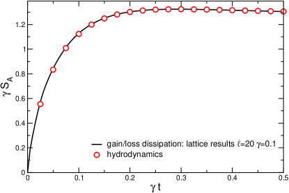
Figure 2: Dynamics of the subsystem von Neumann entropy $S_{A}$ in the Ising chain after a magnetic field quench $h_{0}\to h$ ($h_{0}=0.1,h=2$) in the presence of diagonal gain/loss dissipation. The dissipation corresponds to Kossakowski matrix with $a=b=3/2$ $c=-1/2i$ (cf. (39)), and $\gamma=0.1$. The figure shows $\gamma S_{A}$ versus $\gamma t$. The continuous line denotes exact lattice results. The circles are the theory predictions in the weakly-dissipative hydrodynamic limit $\gamma\to 0$, $t,\ell\to\infty$ with $\gamma\ell$ and $t/\ell$ fixed.

Here we consdier the entropy $S_{A}$ of a finite subsystem $A$ of length $\ell$ embedded in an infinite chain (see Fig. 1). In Fig. 2 we show numerical data for $S_{A}$. We consider the quench from the ground state of the Ising chain with initial magnetic field $h_{0}=0.1$ and final one $h=2$. We focus on gain/loss dissipation (see section 2.3) with gain rate $\gamma g^{+}$ and loss rate $\gamma g^{-}$. We fix $g^{+}=0.5$ and $g^{-}=1$. This corresponds to Kossakowski matrix (39) with $a=b=3/2$ and $c=-1/2i$ This gives $z_{\mathrm{o}}=s_{\mathrm{o}}=0$ (cf. (57) and (44)), implying that, as discussed already, gain/loss dissipation is a particular case of the even dissipation discussed in section 4.1. We should mention that dissipation with non-local losses [18] is even as well. In Fig. 2 we fix the strength of the dissipation $\gamma=0.1$. The continuous black line denotes numerical exact results obtained by using the analytic expression for the time-evolved correlation matrix $\Gamma$ (cf. (16)) and the results in A. The circles in the Figure are the analytic results in the weakly-dissipative hydrodynamic limit (cf. (63)). Although Eq. (63) is expected to hold in the limit $\gamma\to 0$ the agreement between the numerics and the analytic result is remarkable.

Notice that $\gamma S_{A}$ attains a finite value at $\gamma t\to\infty$. This is due to the second term in (63), which is sensitive only to the dissipative processes. On the other hand, the first term in (63) describes the contribution to $S_{A}$ of correlated pairs of quasiparticles, similar to the case without dissipation. As it was discussed in section 4.2 this vanishes at long times. To extract these contributions, it is convenient to focus on the mutual information, as it is clear from (68).

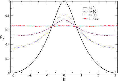
Figure 3: Evolution of quasiparticle densities in the Ising chain with linear dissipation after a magnetic field quench $h_{0}\to h$. All the results are for the $h_{0}=0.1$ and $h=2$. Here we consider diagonal gain/loss dissipation, which corresponds to Kossakowski matrix (cf. (39)) with $a=b=3/2$ and $c=-0.5i$, and $\gamma=0.0125$. $\rho_{k}$ is obtained from (66). The red dashed-dotted line is the result for $t\to\infty$.

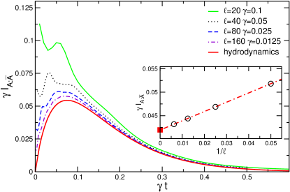
Figure 4: Dynamics of the mutual information ${\mathcal{I}}_{A:\bar{A}}$ in the Ising chain with diagonal gain/loss dissipation after the magnetic field quench $h_{0}\to h$ ($h_{0}=0.1,h=2$). The dissipation corresponds to Kossakowski matrix (cf. (39)) with $a=b=3/2$ $c=-1/2i$ and $\gamma=1/(2\ell)$. In the main figure we plot $\gamma{\mathcal{I}}_{A:\bar{A}}$ versus $\gamma t$. The different lines are exact lattice results for different $\ell$. The continuous red line is the expected result in the weakly-dissipative hydrodynamic limit $\ell,t\to\infty$ with $\gamma\ell$ $\gamma t$ fixed. Scaling corrections due to finite $t,\ell$ are present. Inset: Finite-size scaling analysis. We plot $\gamma{\mathcal{I}}_{A:\bar{A}}$ versus $1/\ell$ at fixed $\gamma t=0.15$. The circles are the same data as in the main Figure, the square symbol at $\ell\to\infty$ is the hydrodynamic limit result. The dashed-dotted line is a linear fit.

5.2 Mutual information

Here we focus on the mutual information ${\mathcal{I}}_{A:\bar{A}}$ between interval $A$ and its complement. As it is clear from (68), the mutual information is solely sensitive to the correlated pairs that are produced after the quench and shared by the bipartition. Specifically, in constructing the mutual information the second term in (63) cancels out. However, the mutual information does not represent a proper measure of entanglement since quasiparticles, in these cases, are both quantum and classically correlated.

We first consider the case of gain/loss dissipation, as in section 5.1. Before discussing the mutual information it is useful to consider the quasiparticle density $\rho_{k}$, which determines (cf. (68)) the dynamics of the mutual information. We plot $\rho_{k}$ in Fig. 3 versus the quasimomentum $k$, for several times after the quench. At $t=0$ one has $\rho_{k}=(1-\cos(\Delta_{k}))/2$. The initial $\rho_{k}$ exhibits a maximum at $k=0$ and it vanishes at $\pm\pi$. At long times $\gamma t\to\infty$, larger momenta get populated, although $\rho_{k}$ is not completely flat in momentum space. The steay-state $\rho_{k}$ is obtained from (72). For gain and loss dissipation with rates $\gamma g^{+}$ and $\gamma g^{-}$ one has $z_{\mathrm{o}}=s_{\mathrm{o}}=0$ and $z_{\mathrm{e}}=-(g^{-}-g^{+})\cos(\theta_{k})$ (cf. (44) (58) (15)), which, together with (72), imply that $\rho_{k}(\infty)=(1-z_{\mathrm{e}}/s_{\mathrm{e}})/2$. Notice that $\rho_{k}$ is an even function of $k$, as expected for even dissipation.

We show numerical results for the mutual information in Fig. 4. We consider the same parameters as in Fig. 2, plotting the rescaled von Neumann mutual information $\gamma{\mathcal{I}}_{A:\bar{A}}$ versus rescaled time $\gamma t$. The strength of the dissipation $\gamma$ is rescaled as $2/\ell$. The red continuous line is the analytic result in the weakly-dissipative hydrodynamic limit (cf. (68)). In contrast with the results for the entropy $S_{A}$ (see Fig. 2), the data for the mutual information exhibit sizeable corrections, with oscillating behavior. At large $\gamma t$ the mutual information decays, as predicted by (68). Eq. (68) is valid only in the weakly-dissipative hydrodynamic limit. Indeed, upon increasing $\ell$ and decreasing $\gamma$, the numerical data approach the theory predictions. This is checked in the inset of Fig. 4, showing $\gamma{\mathcal{I}}_{A}$ versus $1/\ell$ at fixed $\gamma t=0.15$. The dashed-dotted line is a fit to a $1/\ell$ behavior, whereas the full square symbol is the result for $\ell\to\infty$. The agreement with (68) is remarkable. We should mention that similar scaling corrections as $1/\ell$ are present in the case without dissipation [10].

To provide a more stringent check of the results of section 4 we now consider a more complicated dissipation. Specifically, we choose the Kossakowski matrix (cf. (34)) with parameters $c=\sin(k)-1/2i$, $a=b=3/2$. Although the dissipation is non-diagonal, it is still even (see section 4.1).

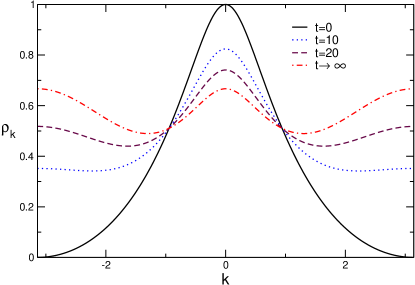
Figure 5: Evolution of quasiparticle densities $\rho_{k}$ in the Ising chain with linear dissipation after a magnetic field quench $h_{0}\to h$. All the results are for the $h_{0}=0.1$ and $h=2$. The Kossakowski matrix (cf. (34)) encoding dissipation has parameters as $a=b=3/2$, $c=\sin(k)-1/2i$, and $\gamma=0.0125$. $\rho_{k}$ is obtained from (66). As in Fig. 4 the dissipation is even. Indeed, one has $\rho_{k}=\rho_{-k}$.

We first discuss the quasiparticles densities $\rho_{k}$ in Fig. 5. The behavior is qualitatively similar to that observed in Fig. 3. The intial density is peaked around $k=0$, and it vanishes at $k=\pm\pi$, whereas at long times quasiparticles with larger $k$ are populated. At $t\to\infty$ the density exhibits oscillating beahavior as a function of $k$, as in Fig. 3.

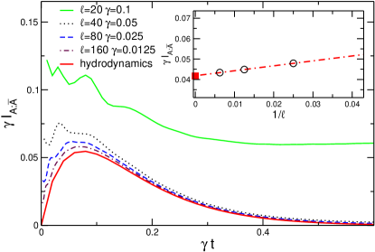
Figure 6: The same as in Figure 8 for the dissipation given by the Kossakowski matrix (cf. (39)) with $a=b=3/2$, $c=\sin(k)-1/2i$, where $k$ is the quasimomentum. The inset show the finite-size scaling analysis for fixed $\gamma t=0.15$.

The mutual information is reported in Fig. 6. The data exhibit oscillating scaling corrections for small $\ell$ and short times. These corrections decay as $1/\ell$. In the hydrodynamic scaling limit the agreement between the numerical data and the quasiparticle picture is perfect, as shown in the inset. Notice that, similar to the gain/loss dissipation (see Fig. 6), the mutual information vanishes at $t\to\infty$, in agreement with the results of section 4.2.

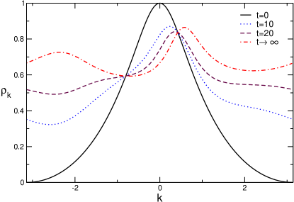
Figure 7: Evolution of the effective quasiparticle densities $\rho_{k}=(1-C_{k}+A_{k})/2$ (cf. (66)) after a quantum quench in the dissipative Ising chain. Results are for the quench with $h_{0}=0.1$ and $h=2$. The dissipation corresponds to Kossakowski matrix (cf (39)) with $a=b=3/2$, $c=5/2\cos(k)-1/2i$, and $\gamma=0.0125$. Notice that $\rho_{k}\neq\rho_{-k}$.

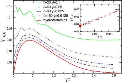
Figure 8: Dynamics of the mutual information ${\mathcal{I}}_{A:\bar{A}}$ in the Ising chain with linear dissipation after the magnetic field quench $h_{0}\to h$ ($h_{0}=0.1,h=2$). The dissipation corresponds to the Kossakowski matrix (cf. (39)) with $a=b=3/2$, $c=5/2\cos(k)-1/2i$, with $k$ the quasimomentum. The dissipation strength $\gamma$ is rescaled as $\gamma=1/(2\ell)$. In the main figure we plot $\gamma{\mathcal{I}}_{A:\bar{A}}$ versus $\gamma t$. Different lines are exact lattice results for different sizes $\ell$ of $A$. The continuous red line is the result in the weakly-dissipative hydrodynamic limit. Scaling corrections due to the finite $t,\ell$ are present. Inset: Finite-size scaling analysis. We plot $\gamma{\mathcal{I}}_{A:\bar{A}}$ versus $1/\ell$ at fixed $\gamma t=0.2$. The circles are the same data as in the main Figure, the square symbol at $\ell\to\infty$ is the hydrodynamic limit result. The dashed-dotted line is a linear fit.

5.3 Evolution under an “unphysical” dissipation

A crucial condition for the Lindblad equation (1) to be physical is that the Kossakowski matrix is positive semidefinite. This is necessary to ensure that the Lindblad evolution is a completely positive and trace-preserving map [20]. Moreover, any fermionic density matrix $\rho$ is characterized by its Majorana covariance matrix $\Gamma$ (cf. (16)). The matrix $\Gamma$ is by definition purely imaginary and antisymmetric, which implies that its eigenvalues are real and are arranged in pairs $\pm\nu_{j}$. The only condition for $\Gamma$ to correspond to a physical density matrix is that $|\nu_{j}|\leq 1$. An interesting observation is that this condition can be satisfied even if the Kossakowski matrix is not positive semidefinite. This could mean that the dynamical map is positive, even if not completely positive, or that it is not even positive but still maps the initial state considered into a well-defined state. Even in these “unphysical” situations the analytical results derived in section 4 hold true.

Here, in order to show this, we consider the Kossakowski matrix with $a=b=3/2$ and $c=5/2\cos(k)-1/2i$. First, now one has that $C_{k}\neq 0$ (cf. (59)). This implies that we are not considering even dissipation. This is shown in Fig. 7. As it is clear from the figure, $\rho_{k}$ is not an even function of $k$. One can check that the eigenvalues of $K$ are not positive. However, we verified numerically that at any time $t$, the eigenvalues of $\Gamma$ satisfy the condition $|\nu_{j}|\leq 1$. The validity of our formulae for this unphysical dissipation is verified in Fig. 8 focusing on the mutual information. Despite the fact that the dissipation is not even, and that the evolution is not a completely positive map, the qualitative behavior of ${\mathcal{I}}_{A:\bar{A}}$ is the same as for the other types of dissipation explored so far. Specifically, the mutual information exhibits a peak at intermediate times and it decays exponentially at $t\to\infty$. Notice, however, the large scaling corrections, which are discussed in the inset of Fig. 8 at fixed $\gamma t=0.2$.

6 Conclusions

We investigated the out-of-equilibrium dynamics after a generic magnetic field quench in the transverse field Ising chain in the presence of the most general linear dissipation that can be treated within the framework of Markovian master equations [41]. Our main result is formula (60), which provides an analytic expression for the dynamics of any function of the Majorana covariance matrix, in the weakly-dissipative hydrodynamic limit. By using (60) we derived exact results for the dynamics of von Neumann and Rényi entropies, and of the associated mutual information, after the quench. This allowed us to prove a conjecture presented recently in Ref. [18] for the case of the Ising chain.

Our work opens several interesting research directions. In this paper we considered fermionic Hamiltonians and Lindblad operators. An interesting direction is to investigate whether the hydrodynamic framework can be extended to spin degrees of freedom, for which the presence of the Jordan-Wigner string is expected to play an important role. Moreover, it would be interesting to consider localized dissipation, as for intstance done in Ref. [52], Ref. [46] or the combination of localized dissipation and driving [53, 54]. One important direction is to try to extend the hydrodyanamic framework to interacting integrable systems. Recent years witnessed encouraging progress in this direction [55, 56, 57, 58, 59, 60, 61, 62, 63, 64, 45, 65, 66]. It would be interesting to understand whether the structure of (63) remains the same for interacting integrable systems. Another possibility in order to assess the effect of interactions could be to use bosonization [67]. A very promising direction is to extend our results to quenches from inhomogeneous initial states. It would be useful to understand whether the approach of Ref. [68] and Ref. [49] can be generalized in the presence of dissipation. Finally, it would interesting to investigate the effects of dissipation in the dynamics of entanglement and of quantum correlations in cellular automaton models, such as the rule 54 chain [69].

7 Acknowledgements

F.C. acknowledges support from the “Wissenschaftler-Rückkehrprogramm GSO/CZS” of the Carl-Zeiss-Stiftung and the German Scholars Organization e.V., as well as through the Deutsche Forschungsgemeinsschaft (DFG, German Research Foundation) under Project No. 435696605. V.A. acknowledges support from the European Research Council under ERC Advanced grant No. 743032 DYNAMINT.

Appendix A Subsystem entropies from the covariance matrix

Entropy-related quantities and their dynamics can be obtained from the correlator $\Gamma$ (cf. (16)) (see Ref. [38]). The single-block reduced density matrix $\rho_{A}$ can be written as

$$\rho_{A}=\frac{1}{2^{\ell}}\sum_{\{\mu\}}\mathrm{Tr}\big{[}\rho w_{1}^{\mu_{1}}w_{2}^{\mu_{2}}\cdots w_{2\ell}^{\mu_{2\ell}}\big{]}w_{2\ell}^{\mu_{2\ell}}\cdots w_{1}^{\mu_{1}}.$$ (77)

Here $w_{i}$ are Majorana fermions (cf. (6)), $\mu_{j}=0,1$, and $\rho$ is the full-system density matrix. The Majorana correlation matrix $\Gamma_{ij}$ is defined as (cf. (16))

$$\Gamma_{ij}:=\mathrm{Tr}(\rho w_{i}w_{j})-\delta_{ij}.$$ (78)

Since Wick’s theorem applies, the reduced density matrix can be recast in the form

$$\rho_{A}=\frac{1}{Z}e^{\frac{1}{4}\sum_{mn}w_{m}Ww_{n}},$$ (79)

where $Z$ ensures the normalization condition $\mathrm{Tr}(\rho_{A})=1$. Here $W$ is related to $\Gamma$ as

$$\tanh\Big{(}\frac{W}{2}\Big{)}=\Gamma_{\ell},$$ (80)

where $\Gamma_{\ell}$ is obtained from $\Gamma_{ij}$ by restricting $i,j\in[1,2\ell]$.

First, by definition the $2\ell\times 2\ell$ matrix $\Gamma$ is purely imaginary and antisymmetric and its eigenvalues are organized in pairs $\pm\nu_{j}$ with $j=1,\dots,\ell$. The Rényi entropies $S^{\scriptscriptstyle(n)}$ are written as

$$S_{A}^{(n)}=\frac{1}{1-n}\sum_{j=1}^{\ell}\ln\Big{[}\Big{(}\frac{1+\nu_{j}}{2}\Big{)}^{n}+\Big{(}\frac{1-\nu_{j}}{2}\Big{)}^{n}\Big{]}.$$ (81)

Note that the sum in (81) is restricted only to half of the eigenvalues of $\Gamma$, for instance the positive ones. The von Neumann entropy is obtained as

$$S_{A}=-\sum_{j=1}^{\ell}\frac{1+\nu_{j}}{2}\ln\Big{(}\frac{1+\nu_{j}}{2}\Big{)}+\frac{1-\nu_{j}}{2}\ln\Big{(}\frac{1-\nu_{j}}{2}\Big{)}.$$ (82)

Appendix B A useful identity for the moments of the symbol of Majorana correlators

Here we provide a useful identiy for the generic $2\times 2$ matrix $\mathbb{M}$ of the form

$$\mathbb{M}(a_{j}):=C\mathds{1}_{2}+A\sigma_{x}+B\sigma_{y}e^{ia_{j}\sigma_{x}}.$$ (83)

Here $\mathds{1}_{2}$ is the $2\times 2$ identity matrix, $\sigma_{\alpha}$ with $\alpha=x,y,z$ the standard Pauli matrices, $A,B,C\in\mathbb{C}$ arbitrary complex constants, and $a_{j}\in\mathbb{R}$ real parameters. Notice that the symbol (59) of the generic Majorana correlation function is of the form (83) after a momentum-independent rotation $U=e^{i\pi\sigma_{z}/4}$. As this rotation is irrelevant for the calculation of the entropy, we are going to neglect it in the following. Let us consider the generic product

$$\Pi_{n}(\{a_{i}\}):=\prod_{j=1}^{n}\mathbb{M}(a_{j}),\quad n\in\mathbb{N}.$$ (84)

For instance, $\Pi_{2}$ is given as

$$\Pi_{2}=\mathbb{M}(a_{1})\mathbb{M}(a_{2})=(C^{2}+A^{2})\mathds{1}_{2}+2CA\sigma_{x}\\ +CB\sigma_{y}(e^{ia_{1}\sigma_{x}}+e^{ia_{2}\sigma_{x}})+B^{2}e^{i(a_{2}-a_{1})\sigma_{x}}+iAB\sigma_{z}(e^{ia_{2}\sigma_{x}}-e^{ia_{1}\sigma_{x}}).$$ (85)

For generic $n$, $\Pi_{n}$ will contain terms proportional to $\mathds{1}_{2}$ and to the Pauli matrices. Upon expanding the product in (84), one obtains the string of operators as

$$\Sigma=\Sigma_{1}\Sigma_{2}\quad\cdots\Sigma_{n},\quad\mathrm{with}\,\Sigma_{j}=\mathds{1}_{2},\sigma_{x},\sigma_{y}e^{ia_{j}\sigma_{x}}.$$ (86)

Let us first consider the situation in which there are terms $\Sigma_{j_{l}}=\sigma_{y}e^{ia_{j_{l}}\sigma_{x}}$, with $1\leq j_{1}<j_{2}<\cdots<j_{l}\in[1,n]$, and $l\in[0,n]$ is the total number of $\sigma_{y}$ terms present in the string. Notice that if $l=0$ the string is proportional either to $\mathds{1}_{2}$ or to $\sigma_{x}$. Let us also define as $z_{k}$ with $k\in[1,l+1]$ the number of $\sigma_{x}$ present between $j_{k}$ and $j_{k-1}$. Notice that $z_{1}$ is the number of $\sigma_{x}$ occurring at positions $k<j_{1}$ and $z_{l+1}$ at positions $k>j_{l}$. Now one can imagine of shifting all the terms $e^{ia_{j_{l}}\sigma_{x}}$ in $\Sigma$ to the right starting from the righmost one. In doing that one can use that

$$e^{ia_{j_{l}}\sigma_{x}}\sigma_{y}=\sigma_{y}e^{-ia_{j_{l}}\sigma_{x}}.$$ (87)

This allows to rewrite $\Sigma$ as

$$\Sigma=\Sigma^{\prime}e^{i\sum_{k=1}^{l}(-1)^{k}a_{j_{k}}}.$$ (88)

The string $\Sigma^{\prime}$ is of the form

$$\Sigma^{\prime}=\sigma_{x}^{z_{1}}\mathds{1}_{2}^{j_{1}-1-z_{1}}\sigma_{y}\sigma_{x}^{z_{2}}\mathds{1}_{2}^{j_{2}-j_{1}-1-z_{2}}\sigma_{y}\cdots\sigma_{y}\sigma_{x}^{z_{l+1}}\mathds{1}_{2}^{n-j_{l}-z_{l+1}}.$$ (89)

By multiplying the string of operators in (89) one obtains

$$\Sigma^{\prime}=(-1)^{\sum_{k}kz_{k}}\sigma_{z,l}$$ (90)

with

$$\sigma_{z,l}:=\left\{\begin{array}[]{cc}\sigma_{y}&z\,\mathrm{even},l\,\mathrm{odd}\\ -\sigma_{x}&z\,\mathrm{odd},l\,\mathrm{even}\\ -i\sigma_{z}&z=l\,\mathrm{odd}\\ \mathds{1}_{2}&z=l\,\mathrm{even}\end{array}\right.$$ (91)

where $l$ is the total number of $\sigma_{y}$ and $z=\sum_{k}z_{k}$. Notice that the operator $\sigma_{z,l}$ that one obtains by contracting the string depends only on $z,l$ and not on the ordering of the operators in the string. We now observe that each term with fixed position $j_{1},\dots,j_{l}$ of $\sigma_{y}$ and a total number $z$ of $\sigma_{x}$ comes with multiplicity ${\mathcal{D}}_{z}(\{j_{l}\})$, which is obtained by summing over all the ways of distributing the $\sigma_{x}$ and the identity matrix $\mathds{1}_{2}$. $\mathcal{D}_{z}$ is given as

$${\mathcal{D}}_{z}(\{j_{l}\}):=\sum_{z_{1},z_{2},\dots,z_{l+1}}(-1)^{\sum_{m}mz_{m}}B^{j_{1},0}_{z_{1}}B^{j_{2,1}}_{z_{2}}\cdots B^{j_{l,l-1}}_{z_{l}}B^{n-j_{l}}_{z_{l+1}}\delta_{z,\sum_{m}z_{m}},$$ (92)

where we defined

$$B^{x}_{y}:=\binom{x}{y},\quad j_{\alpha,\beta}:=j_{\alpha}-j_{\beta}-1,\quad j_{1,0}:=j_{1}-1.$$ (93)

We do not provide the proof of (92), which can be done by induction. We verified numerically for several values of $z$ and $l$ that (92) holds true.

Putting everything together, we obtain that

$$\Pi_{n}(\{a_{i}\})=\frac{1}{2}[(A-C)^{n}+(A+C)^{n}]\mathds{1}_{2}+\frac{1}{2}[(A+C)^{n}-(A-C)^{n}]\sigma_{x}\\ +\sum_{z=0}^{n}\sum_{l=1}^{n-z}\sigma_{z,l}A^{z}B^{l}C^{n-l-z}\sum_{1\leq j_{1}<j_{2}<\cdots<j_{l}\leq n}{\mathcal{D}}_{z}(\{j_{l}\})\exp\Big{(}i\sum_{m=1}^{l}(-1)^{l-m}a_{j_{m}}\sigma_{x}\Big{)},$$ (94)

where $\sigma_{s,l}$ is defined in (91) and ${\mathcal{D}}_{z}$ in (92). The first two terms in (94) arise from contracting the strings of operators $\Sigma$ (cf. (86)) that do not contain any term $e^{ia_{j_{l}}\sigma_{x}}$.

It is useful to consider the situation in which the exponent in the last term in (94) depends only on the total number $l$ of $\sigma_{y}$ but not on the order in which they are placed. This will be relevant in C. We also restrict ourselves to even $n$. Thus, one can replace $j_{l}\to l$ in (94) and perform the sum over $j_{l}$. First, one observes that for both $l,z$ odd the sum vanishes. In the other cases, one can verify that for any fixed $z$ and $l>0$ one has that

$$\sum_{1\leq j_{1}<j_{2}\cdots<j_{l}\leq n}{\mathcal{D}}_{z}(\{j_{l}\})=(-1)^{z}\binom{\lfloor(l+z)/2\rfloor}{\lfloor l/2\rfloor}\binom{n}{l+z}$$ (95)

In summary, one obtains that (94) is rewritten as

$$\Pi_{n}(\{a_{j}\})=\frac{1}{2}[(A-C)^{n}+(A+C)^{n}]\mathds{1}_{2}+\frac{1}{2}[(A+C)^{n}-(A-C)^{n}]\sigma_{x}\\ +\sum_{z=0}^{n}\sum_{l=1}^{n-z}\sigma^{\prime}_{z,l}A^{z}B^{l}C^{n-z-l}\binom{\lfloor(l+z)/2\rfloor}{\lfloor l/2\rfloor}\binom{n}{l+z}\exp\Big{(}i\sum_{m=1}^{l}(-1)^{l-m}a_{m}\sigma_{x}\Big{)},$$ (96)

where $\sigma^{\prime}_{z,l}$ is zero if both $z,l$ are odd, and equal to $\sigma_{z,l}$ (cf. (91)) otherwise. Equation (94) allows us to calculate $\mathrm{Tr}(\Pi_{2n}(a(k)))$. Only the terms with both $l$ and $z$ even survive in the last term in (94). We obtain that

$$\mathrm{Tr}(\Pi_{2n})=(A-C)^{2n}+(A+C)^{2n}\\ +2\sum_{z=0}^{n}\sum_{l=1}^{n-z}A^{2z}B^{2l}C^{2(n-z-l)}\binom{l+z}{l}\binom{2n}{2(l+z)}.$$ (97)

This is rewritten as

$$\mathrm{Tr}(\Pi_{2n})=2\sum_{p=0}^{n}\binom{2n}{2p}(A^{2}+B^{2})^{p}C^{2(n-p)}.$$ (98)

Notice that if $C=0$, which is the case considered in Ref. [32], one obtains the simpler result

$$\mathrm{Tr}(\Pi_{2n})=2(A^{2}+B^{2})^{n}.$$ (99)

Appendix C Hydrodynamic limit for the integer moments of $\Gamma$: Proof of a general formula

In this section we derive a general formula describing the dynamics of the moments of the Majorana covariance matrix $\Gamma_{\ell}$ (see A) restricted to subystem $A$. We consider the case in which the full-system correlator $\Gamma$ is obtained from a symbol $\hat{\Gamma}_{k}$ of the form (59), i.e.,

$$\hat{\Gamma}_{k}=C_{k}\mathds{1}_{2}+A_{k}\sigma^{(k)}_{x}+B_{k}\sigma^{(k)}_{y}e^{ia(k)t\sigma^{(k)}_{x}}.$$ (100)

Here $A_{k},B_{k},C_{k}$ are complex functions of $k$, $a(k)$ is a real function, and $k$ is the quasimomentum. Notice that here we are interested in the case with $C_{k}$ odd function of $k$, whereas $B_{k},A_{k}$ are even functions of $k$ (see section 3). The fact that $C_{k}$ is odd ensures that $\mathrm{Tr}(\Gamma)=0$. However, for the derivation below the functions $A_{k},B_{k},C_{k}$ can be generic. In (100) we introduced the rotated Pauli matrices $\sigma_{\alpha}^{(k)}$, which are defined as

$$\sigma_{\alpha}^{(k)}:=e^{i\boldsymbol{v}(k)\cdot\boldsymbol{\sigma}}\sigma_{\alpha}e^{-i\boldsymbol{v}(k)\cdot\boldsymbol{\sigma}},\quad\alpha=x,y,z.$$ (101)

Here $\boldsymbol{v}(k):=(v_{x},v_{y},v_{y})$ is a vector of arbitrary real functions of $k$. We anticipate that the final result will not depend on the choice of $\boldsymbol{v}$. In the following, to lighten the notation, we are going to omit the dependence on $k$ in $A_{k},B_{k},C_{k}$. Let us now consider the correlation matrix $\Gamma_{rs}$, which is obtained as

$$\Gamma_{rs}=\int_{\pi}^{\pi}\frac{dk}{2\pi}e^{ik(r-s)}\hat{\Gamma}_{k}.$$ (102)

The restricted matrix $\Gamma_{\ell}$ is obtained by considering $r,s\in[1,\ell]$. Here we are interested in the dynamics of the moments of $\Gamma_{\ell}$, which are defined as

$$M_{2n}:=\mathrm{Tr}(\Gamma^{2n}_{\ell}).$$ (103)

Notice that we only consider the even moments of $\Gamma_{\ell}$ because the odd ones are zero by definition. Here we focus on the space-time scaling limit with $t,\ell\to\infty$ with their ratio fixed. The derivation that we are going to discuss is quite similar to Ref. [32]. To proceed we use the trivial identity

$$\sum_{m=1}^{\ell}e^{imk}=\frac{\ell}{4}\int_{-1}^{1}d\xi w(k)e^{i(\ell\xi+\ell+1)k/2},\quad w(k):=\frac{k}{\sin(k/2)}.$$ (104)

From (105), we obtain that

$$\mathrm{Tr}(\Gamma^{2n}_{\ell})=\Big{(}\frac{\ell}{4}\Big{)}^{2n}\int\limits_{[-\pi,\pi]^{2n}}\frac{d^{2n}k}{(2\pi)^{2n}}\int\limits_{[-1,1]^{2n}}d^{2n}\xi D(\{k\})F(\{k\})e^{i\ell\sum_{j=0}^{2n-1}\xi_{j}(k_{j+1}-k_{j})/2},$$ (105)

where we introduced the functions

$$D(\{k\}) =\prod_{j=0}^{2n-1}w(k_{j}-k_{j-1})$$ (106)

$$F(\{k\}) =\mathrm{Tr}\prod_{j=0}^{2n-1}\hat{\Gamma}_{k_{j}}.$$ (107)

Following Ref. [32], it is convenient to change variables as

$$\zeta_{0}=\xi_{1}$$ (108)

$$\zeta_{i}=\xi_{i+1}-\xi_{i},\quad i\in[1,2n-1].$$ (109)

This allows us to rewrite (105) as

$$\mathrm{Tr}(\Gamma^{2n}_{\ell})=\Big{(}\frac{\ell}{4}\Big{)}^{2n}\int\limits_{[-\pi,\pi]^{2n}}\frac{d^{2n}k}{(2\pi)^{2n}}\int_{R_{\xi}}d^{2n}\zeta_{i}D(\{k\})F(\{k\})e^{-i\ell\sum_{j=1}^{2n-1}\zeta_{j}(k_{j}-k_{0})/2},$$ (110)

Here the integration domain for $\zeta_{i}$ is

$$R_{\xi}:-1\leq\sum_{j=0}^{p-1}\zeta_{j}\leq 1,\quad p\in[1,2n].$$ (111)

The integration over $\zeta_{0}$ is trivial because the integrand in(112) does not depend on $\zeta_{0}$. We obtain

$$\mathrm{Tr}(\Gamma^{2n}_{\ell})=\Big{(}\frac{\ell}{4}\Big{)}^{2n}\int\limits_{[-\pi,\pi]^{2n}}\frac{d^{2n}k}{(2\pi)^{2n}}\int d^{2n-1}\zeta_{i}D(\{k\})F(\{k\})e^{-i\ell\sum_{j=1}^{2n-1}\zeta_{j}(k_{j}-k_{0})/2}\mu(\{\zeta\}),$$ (112)

where we introduced the integration measure $\mu$ as

$$\mu(\{\zeta_{j}\})=\max\Big{[}0,\min\limits_{j\in[0,2n-1]}\Big{[}1-\sum_{k=1}^{j}\zeta_{k}\Big{]}+\min\limits_{j\in[0,2n-1]}\Big{[}1+\sum_{k=1}^{j}\zeta_{k}\Big{]}\Big{]}.$$ (113)

The strategy to determine the behaviour of (112) in the space-time scaling limit is to use the stationary phase approximation for the integrals over $k_{1},\dots,k_{2n-1}$ and $\zeta_{1},\dots,\zeta_{2n-1}$. Stationarity with respect to the variables $\zeta_{i}$ in (112) implies that

$$k_{j}\approx k_{0},\quad\forall j\in[1,2n-1].$$ (114)

Now we can replace $k_{j}\to k_{0}$ in the definitions (106) and (107) to obtain

$$F(\{k_{j}\})\to\mathrm{Tr}\prod_{j=0}^{2n-1}\Big{[}C_{k_{0}}\mathds{1}_{2}+A_{k_{0}}\sigma_{x}+B_{k_{0}}\sigma_{y}e^{ia(k_{j})t\sigma_{x}}\Big{]}$$ (115)

$$D(\{k_{j}\})\to 2^{n}.$$ (116)

Notice that in (115) we are not allowed to replace $k_{j}\to k_{0}$ in the phase factor $e^{ia(k_{j})t\sigma_{x}}$, which has to be treated with the stationary phase. In (115) we replaced $\sigma_{\alpha}^{(k)}\to\sigma_{\alpha}$. We now use (94), which allows us to rewrite the product in (115). From (112) we obtain that

$$\mathrm{Tr}(\Gamma^{2n}_{\ell})=\Big{(}\frac{\ell}{2}\Big{)}^{2n}\int\limits_{[-\pi,\pi]^{2n}}\frac{d^{2n}k}{(2\pi)^{2n}}\int d^{2n-1}\zeta_{i}\mu(\{\zeta_{m}\})\mathrm{Tr}\Big{\{}\frac{1}{2}[(A-C)^{2n}+(A+C)^{2n}]\mathds{1}_{2}\\ +\frac{1}{2}[(A+C)^{2n}-(A-C)^{2n}]\sigma_{x}+\sum_{z=0}^{2n}\sum_{l=1}^{2n-z}\sigma_{z,l}A^{z}B^{l}C^{2n-z-l}\\ \times\sum_{1\leq j_{1}<j_{2}<\cdots<j_{l}\leq 2n}\Big{[}{\mathcal{D}}_{z}(\{j_{m}\})\exp\Big{(}i\sum_{m=1}^{l}(-1)^{l-m}a(k_{j_{m}})t\sigma_{x}\Big{)}\Big{]}\Big{\}}e^{-i\ell\sum_{j=1}^{2n-1}\zeta_{j}(k_{j}-k_{0})/2},$$ (117)

where ${\mathcal{D}}_{z}$ and $\sigma_{z,l}$ are defined in (92) It is straightforward to perform the trace of the first two terms in the curly brackets. In the last term in (117) only the cases with both $l$ and $z$ even give a nonzero contribution. Moreover, the last integral in (117) is invariant under permutation of the momenta $k_{j}$. Thus, one can replace $a(k_{j_{m}})\to a(k_{m})$ in the exponential. After using (95) and performing the trace we obtain

$$\mathrm{Tr}(\Gamma^{2n}_{\ell})=\Big{(}\frac{\ell}{2}\Big{)}^{2n}\int\limits_{[-\pi,\pi]^{2n}}\frac{d^{2n}k}{(2\pi)^{2n}}\int d^{2n-1}\zeta_{i}\mu(\{\zeta_{m}\})e^{-i\ell\sum_{j=1}^{2n-1}\zeta_{j}(k_{j}-k_{0})/2}\Big{\{}\\ [(A-C)^{2n}+(A+C)^{2n}]+2\sum_{z=0}^{n}\sum_{l=1}^{n-z}\binom{l+z}{l}\binom{2n}{2(l+z)}A^{2z}B^{2l}C^{2(n-l-z)}\cos\Big{(}\sum_{m=0}^{2l+1}(-1)^{2l-m+1}a(k_{m})t\Big{)}\\ +2i\sum_{z=0}^{n-1}\sum_{l=1}^{n-z-1}\binom{l+z}{l}\binom{2n}{2l+2z+1}A^{2z+1}B^{2l}C^{2n-2z-2l-1}\sin\Big{(}\sum_{m=0}^{2l-1}(-1)^{2l-m+1}a(k_{m})t\Big{)}\Big{\}},$$ (118)

To proceed, we employ the stationary phase approximation to extract the leading behavior of (118) in the limit $\ell,t\to\infty$ with the ratio $t/\ell$ fixed. By rewriting the sine and cosine function in (118) in terms of exponentials, it is clear that one has integrals $\Lambda_{l}$ of the type

$$\Lambda_{l}:=\Big{(}\frac{\ell}{2}\Big{)}^{2n-1}\int\limits_{[-\pi,\pi]^{2n-1}}\frac{d^{2n-1}k}{(2\pi)^{2n-1}}\int d^{2n-1}\zeta_{i}f(k_{0})\\ \exp\Big{(}\pm i\sum_{j=0}^{2l-1}(-1)^{2l-j-1}a(k_{j})t-i\ell\sum_{j=1}^{2n-1}\zeta_{j}(k_{j}-k_{0})/2\Big{)}\mu(\{\zeta_{m}\}),$$ (119)

where $f(k_{0})$ is obtained from (118) by collecting the terms that do not contain complex exponentials. The subscript $l$ in $\Lambda_{l}$ is to stress that $l$ appears in the exponent in (118) and it affects the stationary phase result. The first term in the exponential in (119) is obtained from the cosine and sine functions in (118), whereas the second one is the phase factor in (118).

We are now ready to apply the stationary phase approximation to the integral (119). The stationary phase states that in the limit $\ell\to\infty$ one has [70]

$$\int_{D}d^{N}xp(\boldsymbol{x})e^{i\ell q(\boldsymbol{x})}\rightarrow\Big{(}\frac{2\pi}{\ell}\Big{)}^{N/2}p(\boldsymbol{x}_{0})|\mathrm{det}H|^{-1/2}\exp\Big{[}i\ell q(\boldsymbol{x}_{0})+i\pi\frac{\sigma_{A}}{4}\Big{]}.$$ (120)

Here $p(\boldsymbol{x})$ and $q(\boldsymbol{x})$ are arbitrary functions, $D$ is the integration domain and $\ell$ is a parameter. On the right hand side in (120), $\boldsymbol{x}_{0}$ is the stationary point satisfying $\boldsymbol{\nabla}q(\boldsymbol{x}_{0})=0$. In (120) $H$ is the hessian matrix $H=\partial_{x_{i}}\partial_{x_{j}}q(\boldsymbol{x})$, and $\sigma$ its signature, i.e., the difference between the number of positive and negative eigenvalues of $H$.

From (119), in the hydrodynamic limit $\ell,t\to\infty$ with their ratio fixed, the stationary phase approximation in the variables $k_{1},\dots,k_{2n-1}$ and $\zeta_{1},\dots,\zeta_{2n-1}$ is determined by the stationary points

$$\bar{k}_{j}=k_{0} j=1,\dots,2n-1$$ (121)

$$\bar{\zeta}_{j}=\pm 2\frac{t}{\ell}(-1)^{j}a^{\prime}(k_{j}) j=1,\dots,2l-1$$ (122)

$$\bar{\zeta}_{j}=0 j=2l,\dots,2n-1,$$ (123)

where the $\pm$ in (122) originates from the first term in the exponent in (119). From (113), one obtains thata at the stationary point

$$\bar{\mu}(\{\bar{\zeta}_{j}\})=\left\{\begin{array}[]{cc}\frac{2}{\ell}\max[0,\ell-|a^{\prime}(k_{0})|t]&l\neq 0\\ 2&l=0\end{array}\right.$$ (124)

Importantly, Eq. (124) does not depend on the $\pm$ sign of $\bar{\zeta}_{j}$ in (122).

To proceed, we observe that in our case $\mathrm{det}(H)=4^{1-2n}$ (cf. (120)). Moreover, the signature $\sigma$ is always zero, and the phase factor (120) does not contribute because the alternating sum in the exponent in (120) has an even number of terms. Crucially, since $\bar{\mu}(\{\bar{\zeta}_{m}\})$ does not depend on the sign in (122), the last term in (118) vanishes. Finally, we obtain that

$$\mathrm{Tr}(\Gamma^{2n}_{\ell})=\ell\int\frac{dk}{2\pi}[(A-C)^{2n}+(A+C)^{2n}]\\ +2\sum_{z=0}^{n}\sum_{l=1}^{n-z}\binom{l+z}{l}\binom{2n}{2(l+z)}\int\frac{dk}{2\pi}A^{2z}B^{2l}C^{2(n-l-z)}\max(0,\ell-|a^{\prime}|t).$$ (125)

Here we redefined $k_{0}\to k$. For $C=0$ one recovers the result of Ref. [32]. Eq. (125) can be conveniently rewritten as

$$\mathrm{Tr}(\Gamma^{2n}_{\ell})=\int\frac{dk}{2\pi}[(A-C)^{2n}+(A+C)^{2n}]\min(\ell,|a^{\prime}|t)\\ +2\sum_{z=0}^{n}\binom{2n}{2z}\int\frac{dk}{2\pi}(A^{2}+B^{2})^{z}C^{2(n-z)}\max(0,\ell-|a^{\prime}|t).$$ (126)

Equivalently, one can rewrite (126) as

$$\mathrm{Tr}(\Gamma^{2n}_{\ell})=\int\frac{dk}{2\pi}[(A-C)^{2n}+(A+C)^{2n}]\min(\ell,|a^{\prime}|t)\\ +\int\frac{dk}{2\pi}\mathrm{Tr}(\Gamma_{L}^{2n})\max(0,\ell-|a^{\prime}|t).$$ (127)

In the second row in (127) we used (98) to identify the trace of the moments of the full-system correlator $\Gamma_{L}$. Eq. (127) implies that for a generic function ${\mathcal{F}}(z)$, one has that

$$\mathrm{Tr}({\mathcal{F}}(\Gamma^{2}_{\ell}))=\int\frac{dk}{2\pi}[{\mathcal{F}}((A-C)^{2})+{\mathcal{F}}((A+C)^{2})]\min(\ell,|a^{\prime}|t)\\ +\int\frac{dk}{2\pi}\mathrm{Tr}({\mathcal{F}}(\Gamma_{L}^{2}))\max(0,\ell-|a^{\prime}|t).$$ (128)

Eq. (128) is equivalent to (60) after replacing $a(k)=2\varepsilon_{h}(k)$ (cf. (13)).

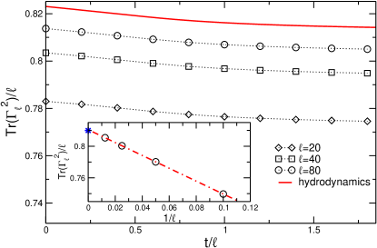
Figure 9: Numerical check of Eq. (127) for $n=1$. We plot $\mathrm{Tr}(\Gamma_{\ell}^{2n})/\ell$ versus $t/\ell$. The functions $A_{k},B_{k},C_{k}$ are defined in (129)-(131). Here we choose $a(k)=2\cos(k)$. The symbols are exact lattice results for different subsystem sizes $\ell$. The continuous red line is the result in the scaling limit $\ell,t\to\infty$ with $t/\ell$ fixed. Finite-size and finite-time corrections are visible. Scaling corrections are investigated in the inset plotting $\mathrm{Tr}(\Gamma_{\ell}^{2n})/\ell$ versus $1/\ell$ at fixed $t/\ell=0.4$. The star symbol is the result in the hydrodynamic limit $\ell\to\infty$. The dashed-dotted line is a linear fit.

It is important to check the validity of (128). In Fig. 9 we discuss some numerical checks of (128) for the second moment $\mathrm{Tr}(\Gamma_{\ell}^{2})$ of $\Gamma_{\ell}$. We consider the fermionic correlator $\Gamma$ of the form (59) with

$$A_{k}=0.87\cos(k)$$ (129)

$$B_{k}=0.1235\cos^{2}(k)$$ (130)

$$C_{k}=0.234\sin(k).$$ (131)

We also fix $a(k)=2\cos(k)$. The symbols in Fig. 9 are exact numerical data for finite $\ell$ and $t$. Since we are interested in the space-time scaling limit, in the figure we plot $\mathrm{Tr}(\Gamma_{\ell}^{2})/\ell$ versus $t/\ell$. The continuous line in Fig. 9 is the result (127) for $n=1$. As it is clear from the figure the data exhibit strong finite-size and finite-time corrections. However, upon increasing $\ell$ they approach the analytic result (127). A more systematic analysis of the scaling corrections is presented in the inset of Fig. 9, showing $\mathrm{Tr}(\Gamma_{\ell}^{2})/\ell$ versus $1/\ell$ at fixed $t/\ell=0.4$. The star symbol in the inset is the expected result in the hydrodynamic limit. The dashed-dotted line is a linear fit. The quality of the fit confirms the validity of (127) and suggests that the corrections are ${\mathcal{O}}(1/\ell)$. Similar corrections are observed also in the case without dissipation [11].

References

References

- [1] Oh C, Noh K, Fefferman B and Jiang L 2021 Classical simulation of lossy boson sampling using matrix product operators (Preprint 2101.11234)
- [2] Zhou Y, Stoudenmire E M and Waintal X 2020 Phys. Rev. X 10(4) 041038 URL https://link.aps.org/doi/10.1103/PhysRevX.10.041038
- [3] Islam R, Ma R, Preiss P M, Eric Tai M, Lukin A, Rispoli M and Greiner M 2015 Nature 528 77–83 ISSN 1476-4687 URL https://doi.org/10.1038/nature15750
- [4] Kaufman A M, Tai M E, Lukin A, Rispoli M, Schittko R, Preiss P M and Greiner M 2016 Science 353 794–800 ISSN 0036-8075 (Preprint https://science.sciencemag.org/content/353/6301/794.full.pdf) URL https://science.sciencemag.org/content/353/6301/794
- [5] Brydges T, Elben A, Jurcevic P, Vermersch B, Maier C, Lanyon B P, Zoller P, Blatt R and Roos C F 2019 Science 364 260–263 ISSN 0036-8075 (Preprint https://science.sciencemag.org/content/364/6437/260.full.pdf) URL https://science.sciencemag.org/content/364/6437/260
- [6] Elben A, Kueng R, Huang H Y R, van Bijnen R, Kokail C, Dalmonte M, Calabrese P, Kraus B, Preskill J, Zoller P and Vermersch B 2020 Phys. Rev. Lett. 125(20) 200501 URL https://link.aps.org/doi/10.1103/PhysRevLett.125.200501
- [7] Rossini D and Vicari E 2021 Coherent and dissipative dynamics at quantum phase transitions (Preprint 2103.02626)
- [8] Calabrese P and Cardy J 2005 Journal of Statistical Mechanics: Theory and Experiment 2005 P04010 URL https://doi.org/10.1088{%}2F1742-5468{%}2F2005{%}2F04{%}2Fp04010
- [9] Fagotti M and Calabrese P 2008 Phys. Rev. A 78(1) 010306 URL https://link.aps.org/doi/10.1103/PhysRevA.78.010306
- [10] Alba V and Calabrese P 2017 Proceedings of the National Academy of Sciences 114 7947–7951 ISSN 0027-8424 (Preprint https://www.pnas.org/content/114/30/7947.full.pdf) URL https://www.pnas.org/content/114/30/7947
- [11] Alba V and Calabrese P 2018 SciPost Phys. 4(3) 17 URL https://scipost.org/10.21468/SciPostPhys.4.3.017
- [12] Alba V and Calabrese P 2017 Phys. Rev. B 96(11) 115421 URL https://link.aps.org/doi/10.1103/PhysRevB.96.115421
- [13] Alba V and Calabrese P 2017 Journal of Statistical Mechanics: Theory and Experiment 2017 113105 URL https://doi.org/10.1088/1742-5468/aa934c
- [14] Mestyán M, Alba V and Calabrese P 2018 Journal of Statistical Mechanics: Theory and Experiment 2018 083104 URL https://doi.org/10.1088/1742-5468/aad6b9
- [15] Alba V and Calabrese P 2019 EPL (Europhysics Letters) 126 60001 URL https://doi.org/10.1209/0295-5075/126/60001
- [16] Maity S, Bandyopadhyay S, Bhattacharjee S and Dutta A 2020 Phys. Rev. B 101(18) 180301 URL https://link.aps.org/doi/10.1103/PhysRevB.101.180301
- [17] Alba V and Carollo F 2021 Phys. Rev. B 103(2) L020302 URL https://link.aps.org/doi/10.1103/PhysRevB.103.L020302
- [18] Carollo F and Alba V 2021 Emergent dissipative quasi-particle picture in noninteracting markovian open quantum systems (Preprint 2106.11997)
- [19] Cao X, Tilloy A and Luca A D 2019 SciPost Phys. 7(2) 24 URL https://scipost.org/10.21468/SciPostPhys.7.2.024
- [20] Breuer H P and Petruccione F 2002 The theory of open quantum systems (Great Clarendon Street: Oxford University Press)
- [21] Amico L, Fazio R, Osterloh A and Vedral V 2008 Rev. Mod. Phys. 80(2) 517–576 URL https://link.aps.org/doi/10.1103/RevModPhys.80.517
- [22] Calabrese P, Cardy J and Doyon B 2009 Journal of Physics A: Mathematical and Theoretical 42 500301 URL https://doi.org/10.1088/1751-8121/42/50/500301
- [23] Laflorencie N 2016 Physics Reports 646 1–59 ISSN 0370-1573 quantum entanglement in condensed matter systems URL https://www.sciencedirect.com/science/article/pii/S0370157316301582
- [24] Devetak I and Winter A 2005 Proceedings of the Royal Society A: Mathematical, Physical and Engineering Sciences 461 207–235 (Preprint %****␣isingdiss_v3.bbl␣Line␣125␣****https://royalsocietypublishing.org/doi/pdf/10.1098/rspa.2004.1372) URL https://royalsocietypublishing.org/doi/abs/10.1098/rspa.2004.1372
- [25] Vidal G and Werner R F 2002 Phys. Rev. A 65(3) 032314 URL https://link.aps.org/doi/10.1103/PhysRevA.65.032314
- [26] Plenio M B 2005 Phys. Rev. Lett. 95(9) 090503 URL https://link.aps.org/doi/10.1103/PhysRevLett.95.090503
- [27] Wichterich H, Molina-Vilaplana J and Bose S 2009 Phys. Rev. A 80(1) 010304 URL https://link.aps.org/doi/10.1103/PhysRevA.80.010304
- [28] Calabrese P, Cardy J and Tonni E 2012 Phys. Rev. Lett. 109(13) 130502 URL https://link.aps.org/doi/10.1103/PhysRevLett.109.130502
- [29] Eisler V and Zimborás Z 2015 New Journal of Physics 17 053048 URL https://doi.org/10.1088/1367-2630/17/5/053048
- [30] Shapourian H and Ryu S 2019 Phys. Rev. A 99(2) 022310 URL https://link.aps.org/doi/10.1103/PhysRevA.99.022310
- [31] Alba V, Bertini B, Fagotti M, Piroli L and Ruggiero P 2021 Generalized-hydrodynamic approach to inhomogeneous quenches: Correlations, entanglement and quantum effects (Preprint 2104.00656)
- [32] Calabrese P, Essler F H L and Fagotti M 2012 Journal of Statistical Mechanics: Theory and Experiment 2012 P07016 ISSN 1742-5468 URL http://dx.doi.org/10.1088/1742-5468/2012/07/P07016
- [33] Polkovnikov A, Sengupta K, Silva A and Vengalattore M 2011 Rev. Mod. Phys. 83(3) 863–883 URL https://link.aps.org/doi/10.1103/RevModPhys.83.863
- [34] Calabrese P, Essler F H L and Mussardo G 2016 Journal of Statistical Mechanics: Theory and Experiment 2016 064001 URL https://doi.org/10.1088/1742-5468/2016/06/064001
- [35] Vidmar L and Rigol M 2016 Journal of Statistical Mechanics: Theory and Experiment 2016 064007 URL https://doi.org/10.1088/1742-5468/2016/06/064007
- [36] Essler F H L and Fagotti M 2016 Journal of Statistical Mechanics: Theory and Experiment 2016 064002 URL https://doi.org/10.1088/1742-5468/2016/06/064002
- [37] Sachdev S 2011 Quantum Phase Transitions 2nd ed (Cambridge University Press)
- [38] Peschel I and Eisler V 2009 Journal of physics a: mathematical and theoretical 42 504003
- [39] Calabrese P, Essler F H L and Fagotti M 2012 Journal of Statistical Mechanics: Theory and Experiment 2012 P07022 ISSN 1742-5468 URL http://dx.doi.org/10.1088/1742-5468/2012/07/P07022
- [40] Caux J S and Essler F H L 2013 Phys. Rev. Lett. 110(25) 257203 URL https://link.aps.org/doi/10.1103/PhysRevLett.110.257203
- [41] Prosen T 2008 New Journal of Physics 10 43026 URL https://doi.org/10.1088/1367-2630/10/4/043026
- [42] Gorini V, Kossakowski A and Sudarshan E C G 1976 Journal of Mathematical Physics 17 821–825 (Preprint https://aip.scitation.org/doi/pdf/10.1063/1.522979) URL https://aip.scitation.org/doi/abs/10.1063/1.522979
- [43] Lindblad G 1976 Communications in Mathematical Physics 48 119–130 ISSN 1432-0916 URL https://doi.org/10.1007/BF01608499
- [44] Nigro D, Rossini D and Vicari E 2019 Phys. Rev. A 100(5) 052108 URL https://link.aps.org/doi/10.1103/PhysRevA.100.052108
- [45] Bouchoule I, Doyon B and Dubail J 2020 SciPost Phys. 9(4) 44 URL https://scipost.org/10.21468/SciPostPhys.9.4.044
- [46] Alba V 2021 Unbounded entanglement production via a dissipative impurity (Preprint 2104.10921)
- [47] Modak R, Alba V and Calabrese P 2020 Journal of Statistical Mechanics: Theory and Experiment 2020 083110 URL https://doi.org/10.1088/1742-5468/aba9d9
- [48] Alba V 2018 Phys. Rev. B 97(24) 245135 URL https://link.aps.org/doi/10.1103/PhysRevB.97.245135
- [49] Alba V, Bertini B and Fagotti M 2019 SciPost Phys. 7(1) 5 URL https://scipost.org/10.21468/SciPostPhys.7.1.005
- [50] Alba V 2019 Phys. Rev. B 99(4) 045150 URL https://link.aps.org/doi/10.1103/PhysRevB.99.045150
- [51] Mestyán M and Alba V 2020 SciPost Phys. 8(4) 55 URL https://scipost.org/10.21468/SciPostPhys.8.4.055
- [52] Alba V and Carollo F 2021 Noninteracting fermionic systems with localized dissipation: Exact results in the hydrodynamic limit (Preprint 2103.05671)
- [53] Turkeshi X and Schiro M 2021 Diffusion and thermalization in a boundary-driven dephasing model (Preprint 2106.13180)
- [54] Yamanaka K and Sasamoto T 2021 Exact solution for the lindbladian dynamics for the open xx spin chain with boundary dissipation (Preprint 2104.11479)
- [55] de Leeuw M, Paletta C and Pozsgay B 2021 Constructing integrable lindblad superoperators (Preprint 2101.08279)
- [56] Hutsalyuk A and Pozsgay B 2021 Integrability breaking in the one dimensional bose gas: Atomic losses and energy loss (Preprint 2012.15640)
- [57] Medvedyeva M V, Essler F H L and Prosen T 2016 Phys. Rev. Lett. 117(13) 137202 URL https://link.aps.org/doi/10.1103/PhysRevLett.117.137202
- [58] Essler F H L and Piroli L 2020 Phys. Rev. E 102(6) 062210 URL https://link.aps.org/doi/10.1103/PhysRevE.102.062210
- [59] Ziolkowska A A and Essler F H 2020 SciPost Phys. 8(3) 44 URL https://scipost.org/10.21468/SciPostPhys.8.3.044
- [60] Bastianello A, De Nardis J and De Luca A 2020 Phys. Rev. B 102(16) 161110 URL https://link.aps.org/doi/10.1103/PhysRevB.102.161110
- [61] Friedman A J, Gopalakrishnan S and Vasseur R 2020 Phys. Rev. B 101(18) 180302 URL https://link.aps.org/doi/10.1103/PhysRevB.101.180302
- [62] Vernier E 2020 SciPost Phys. 9(4) 49 URL https://scipost.org/10.21468/SciPostPhys.9.4.049
- [63] Popkov V, Prosen T and Zadnik L 2020 Phys. Rev. E 101(4) 042122 URL https://link.aps.org/doi/10.1103/PhysRevE.101.042122
- [64] Popkov V, Prosen T and Zadnik L 2020 Phys. Rev. Lett. 124(16) 160403 URL https://link.aps.org/doi/10.1103/PhysRevLett.124.160403
- [65] Buca B, Booker C, Medenjak M and Jaksch D 2020 Dissipative bethe ansatz: Exact solutions of quantum many-body dynamics under loss (Preprint 2004.05955)
- [66] Popkov V and Presilla C 2021 Phys. Rev. Lett. 126(19) 190402 URL https://link.aps.org/doi/10.1103/PhysRevLett.126.190402
- [67] Bácsi A, Moca C P, Zaránd G and Dóra B 2020 Phys. Rev. Lett. 125(26) 266803 URL https://link.aps.org/doi/10.1103/PhysRevLett.125.266803
- [68] Bertini B, Fagotti M, Piroli L and Calabrese P 2018 Journal of Physics A: Mathematical and Theoretical 51(39) 39LT01 ISSN 1751-8113 URL https://iopscience.iop.org/article/10.1088/1751-8121/aad82e
- [69] Klobas K, Bertini B and Piroli L 2021 Phys. Rev. Lett. 126(16) 160602 URL https://link.aps.org/doi/10.1103/PhysRevLett.126.160602
- [70] Wong R 2001 Asymptotic Approximations of Integrals (Society for Industrial and Applied Mathematics) URL https://epubs.siam.org/doi/abs/10.1137/1.9780898719260