Coherent and dissipative dynamics at quantum phase transitions

Abstract

The many-body physics at quantum phase transitions shows a subtle interplay between quantum and thermal fluctuations, emerging in the low-temperature limit. In this review, we first give a pedagogical introduction to the equilibrium behavior of systems in that context, whose scaling framework is essentially developed by exploiting the quantum-to-classical mapping and the renormalization-group theory of critical phenomena at continuous phase transitions. Then we specialize to protocols entailing the out-of-equilibrium quantum dynamics, such as instantaneous quenches and slow passages across quantum transitions. These are mostly discussed within dynamic scaling frameworks, obtained by appropriately extending the equilibrium scaling laws. We review phenomena at first-order quantum transitions as well, whose peculiar scaling behaviors are characterized by an extreme sensitivity to the boundary conditions, giving rise to exponentials or power laws for the same bulk system. In the last part, we cover aspects related to the effects of dissipative interactions with an environment, through suitable generalizations of the dynamic scaling at quantum transitions. The presentation is limited to issues related to, and controlled by, the quantum transition developed by closed many-body systems, treating the dissipation as a perturbation of the critical regimes, as for the temperature at the zero-temperature quantum transition. We focus on the physical conditions giving rise to a nontrivial interplay between critical modes and various dissipative mechanisms, generally realized when the involved mechanism excites only the low-energy modes of the quantum transitions.

1 Plan of the review

1.1 Introduction

The quantum evolution of many-body systems has been considered a challenging problem for long time. The recent experimental progress in the realization, control, and readout of the coherent dynamics of (quasi) isolated, strongly correlated, quantum systems has made this issue particularly relevant for experiments and realizations of physical devices for quantum computing.

Quantum phase transitions (or, more compactly, quantum transitions) separating different phases of closed systems are striking signatures of many-body collective behaviors (see [1] for an introduction to this issue). They are essentially related to the properties of the low-energy spectrum of the system, and in particular the ground state. They give rise to notable long-range quantum correlations and scaling behaviors similar to those observed at classical phase transitions. These emerging critical scenarios entail corresponding out-of-equilibrium phenomena around the quantum transition. Indeed the universal features of the quantum transitions could also be probed by out-of-equilibrium dynamic protocols, for example analyzing the effects of changes of the Hamiltonian parameters across them, which may be instantaneous or extremely slow. The out-of-equilibrium dynamics at quantum transitions can be also addressed within dynamic scaling frameworks, which allow us to identify the critical regimes controlled by the global and universal properties of the quantum transition, such as the nature of the order parameter and the associated symmetry-breaking pattern.

Phenomena related to quantum transitions are important to understand the physics behind several low-energy situations, which include fermionic and bosonic gases, atomic systems in optical lattices, high-Tc superconductivity, quantum-Hall systems, low lying magnetic and spin fluctuations of some insulators and crystals, such as heavy fermion compounds, etc. (see, e.g., Refs. [1, 2] and references therein).

We review issues related to the equilibrium and out-of-equilibrium dynamics of many-body systems at quantum transitions. They are mostly discussed within dynamic scaling frameworks, which have been essentially developed by exploiting the quantum-to-classical mapping and the renormalization-group theory of critical phenomena at continuous phase transitions. In this context, first-order quantum transitions are addressed as well, with emphasis on the dynamic scaling behaviors emerging in finite-size systems: these appear even more complex than those at continuous quantum transitions, due to their extreme sensitivity to the boundary conditions, which may give rise to exponentials or power laws for the same bulk system.

We also cover aspects related to the effects of dissipative interactions with an environment, which are unavoidable in actual experiments. The analysis of dissipative perturbations is presented within appropriate extensions of the dynamic scaling framework at quantum transitions, allowing us to identify a low-dissipation regime where the dissipative perturbations can be incorporated into an extended dynamic scaling theory controlled by the universality class of the quantum transition of the isolated system. We limit our presentation to issues related to, and controlled by, the quantum transition developed by closed many-body systems, treating dissipative mechanisms as perturbations, like the temperature at the zero-temperature quantum transition. In other words, we will not treat dynamic critical phenomena arising from the dissipative mechanism itself. The outlined dynamic scaling framework, even the one extended to allow for dissipative mechanisms, applies when the involved mechanism excites only the low-energy critical modes of the quantum transitions: hereafter we will essentially focus on the corresponding perturbed critical regimes.

To be more precise, we consider dynamical phenomena emerging in the critical regimes of quantum-many body systems, i.e., when the Hamiltonian driving the unitary dynamics is close to a quantum transition and only low-energy critical modes are effectively excited. Within this regime, dynamic scaling frameworks, similar to those developed for equilibrium quantum criticality, provide valuable insight for out-of-equilibrium quantum evolutions as well, such as when quenching the Hamiltonian parameters and/or in the presence of dissipative perturbations. A full understanding of the nonequilibrium quantum dynamics in more general conditions calls for further tools and concepts, which are currently object of intensive investigation.

1.2 Plan

This review focuses on the quantum dynamics of many-body systems close to continuous or first-order quantum transitions (CQTs and FOQTs, respectively), separating their zero-temperature quantum phases. The review can be divided into three parts: In sections 2-7, we discuss the equilibrium features of quantum transitions (QTs). Sections 8-11 deal with the out-of-equilibrium unitary dynamics, controlled by the global and universal properties of the QTs. In the last sections 12-15, we extend the analysis to quantum systems subject to dissipative interactions with an environment, discussing the effects of their perturbations when the many-body systems are close to a QT. The detailed plan of the review follows.

• In Sec. 2, we begin with a compact introduction to QTs, distinguishing between CQTs and FOQTs. We outline their main features, such as the typical universal power laws characterizing continuous transitions, and the infinite-volume discontinuities of the first-order transitions. We discuss the Landau-Ginzburg-Wilson (LGW) framework to study critical phenomena, and some examples of QTs which may depart from this scenario, such as the so-called topological transitions.

• In Sec. 3 we present a number of prototypical models undergoing CQTs and FOQTs, useful to place the quantum phenomena discussed in this review into concrete grounds. We introduce quantum Ising-like or XY systems, discussing their quantum phase diagram and the nature of their transitions; in the case of one-dimensional (1$d$) models, we comment on their relation with the Kitaev fermionic wire. We also present other physically interesting systems, such as Bose-Hubbard (BH) models, with their bosonic condensation phenomena and Mott phases, as well as quantum rotor and Heisenberg spin models.

• In Sec. 4 we outline the scaling theory describing the universal behaviors of systems at CQTs, in equilibrium conditions around the quantum critical point (QCP). For this purpose, the quantum-to-classical mapping and the renormalization-group (RG) theory of critical phenomena are employed as guiding ideas. We present a detailed analysis of the RG scaling ansatz in the thermodynamic limit and in the finite-size scaling (FSS) limit. We also extend the theory to the case the system is subject to an external inhomogeneous potential, such as for trapped particle gases in cold-atom experiments.

• In Sec. 5 we outline the appropriate scaling theory for FOQTs in equilibrium conditions. In particular, we discuss how systems at FOQTs develop a peculiar FSS, characterized by an extreme sensitivity to the boundary conditions (BC), which may give rise to exponential or power-law behaviors with respect to the system size. We provide a unified view of the FSS at QTs, including both CQTs and FOQTs, for which the main difference between CQTs and FOQTs is essentially related to their sensitivity to the BC. The latter feature of FOQTs lies at the basis of the existence of CQTs induced by localized defects, whose tuning can change the bulk phase, unlike the standard scenarios at CQTs.

• In Sec. 6 we present an overview of some concepts founded on the recently developing quantum information science, which have been proven useful to spotlight the presence of singularities at QTs in many-body systems, such as the ground-state fidelity, the Loschmidt amplitude, the quantum Fisher information, various indicators of quantum correlations (as entanglement or quantum discord), etc.

• In Sec. 7 we discuss the behaviors of the quantum-information related quantities introduced in Sec. 6 at CQTs and FOQTs, showing that they present peculiar scaling behaviors, in particular focusing on the ground-state fidelity and the bipartite entanglement.

• Sec. 8 is the first of the sections dedicated to the out-of-equilibrium quantum dynamics at QTs. We outline the dynamic scaling theory describing the out-of-equilibrium dynamics arising from soft instantaneous quantum quenches at CQTs, when only critical low-energy modes get excited by the process. For this purpose, we assume a general hypothesis of homogeneous scaling laws, which are then specialized to the thermodynamic limit and the FSS limit. Beside the standard quantum correlations of local operators, we discuss the behavior of more complex quantities such as the Loschmidt echo, the work fluctuations, the bipartite entanglement. We finally shed light on the possible signatures of QTs in hard quantum quenches, where excitations with higher energy are also involved in the process.

• Sec. 9 deals with another class of dynamic protocols, where the Hamiltonian parameters are slowly changed across CQTs, analogous to those considered to generate the so-called Kibble-Zurek (KZ) mechanism, related to the abundance of defects after crossing a CQT. Starting again from a set of dynamic homogeneous scaling laws, we outline the corresponding dynamic KZ scaling theory in the thermodynamic limit and in the FSS limit, controlled by the universality class of the underlying CQT. This describes the growth of an out-of-equilibrium dynamics even in the limit of very slow changes of the Hamiltonian parameters, because large-scale modes are unable to equilibrate as the system changes phase. We also overview the analytical and numerical evidence of the KZ scaling theory, reported in the literature.

• In Sec. 10 we extend the out-of-equilibrium dynamic scaling theory to FOQTs: analogously as at equilibrium, the dynamic behavior across a FOQT is dramatically sensitive to the BC, giving rise to nonequilibrium evolutions with exponential or power-law time scales (unlike CQTs, where the time scaling is generally independent of the type of boundaries). We address both soft quantum quenches and slow KZ protocols. We also discuss the conditions under which the system at the FOQT effectively behaves rigidly as a few-level quantum system.

• In Sec. 11 we begin considering decoherence phenomena, which generally arise when a given quantum system interacts with an environmental many-body system. We start from the simplest central spin model, describing a single qubit interacting with a many-body system. We discuss how the decoherence dynamics develops when the many-body system is close to a QT, emphasizing the qualitative changes with respect to systems in normal conditions. Again, the analysis is essentially developed within a dynamic scaling framework.

• Sec. 12 is the first of a series of sections discussing the behavior of quantum systems in the presence of dissipative interactions with an environment. We introduce the so-called Lindblad framework allowing for the dissipation through a system-bath coupling scheme that respects some assumptions (typically based on the weak coupling approximation). These lead to a well behaved Markovian master equation for the density matrix operator of the system.

• In Sec. 13 we address the effects of dissipative interactions on the out-of-equilibrium dynamics of systems at QTs, both CQTs and FOQTs. We discuss how the dynamic scaling theory of closed systems can be extended to take into account the perturbations arising from the dissipative interactions. We concentrate on the effects emerging at quantum quenches, identifying a low-dissipation regime where a dissipative dynamic scaling behavior emerges as well.

• In Sec. 14 we extend the discussion to slow KZ-like protocols. In particular, we describe the conditions under which a dynamic KZ scaling behavior can be still observed, even in the presence of dissipation, showing that this requires a particular low-dissipation limit.

• Sec. 15 deals with the effects of local measurements on systems at QTs. This issue is discussed within a dynamic scaling framework, which shows that a peculiar dynamic scaling behavior emerges even in the presence of such type of decoherence perturbations, that is controlled by the universality class of the CQT.

• The concluding Sec. 16 contains a brief summary of this review, with possible motivations that could stimulate new experimental investigations in the field of quantum many-body physics. A brief list of the envisioned platforms where such studies are possible is finally presented.

We shall emphasize that the topics covered in this review deal with phenomena that genuinely arise from the existence of a QT in closed many-body systems. On top of that, we consider general mechanisms, such as dissipative interactions or local measurements, that may destroy the critical features of the QTs, and discuss the regimes when they act as a perturbation that can only effectively excite the low-energy critical modes of the underlying quantum transition bringing them out of equilibrium. As a consequence, some interesting and flourishing issues in the realm of quantum many-body physics will not be touched. We warmly direct the interested reader to the good and recent review papers cited below.

ANNNI	anisotropic next-to-nearest neighbor Ising	LDA	local density approximation
ABC	antiperiodic boundary conditions	LOCC	local operations and classical communication
BKT	Berezinskii-Kosterlitz-Thouless	MC	Monte Carlo
BEC	Bose-Einstein condensation	MI	Mott insulator
BH	Bose-Hubbard	NPRG	nonperturbative renormalization-group
BC	boundary conditions	1$d$	one-dimensional
CFT	conformal field theory	OBC	open boundary conditions
CQT	continuous quantum transition	OFBC	opposite and fixed boundary conditions
DMRG	density-matrix renormalization group	PBC	periodic boundary conditions
ETH	eigenstate thermalization hypothesis	QCP	quantum critical point
EPR	Einstein-Podolsky-Rosen	QED	quantum electrodynamics
EFBC	equal and fixed boundary conditions	QT	quantum transition
FSS	finite-size scaling	QLRO	quasi-long-range order
FOQT	first-order quantum transition	RG	renormalization-group
FBC	fixed boundary conditions	SFT	statistical field theory
GKLS	Gorini-Kossakowski-Lindblad-Sudarshan	3$d$	three-dimensional
HI	Haldane insulator	TSS	trap-size scaling
HT	high-temperature	2$d$	two-dimensional
KZ	Kibble-Zurek	VBS	valence-bond-solid
LGW	Landau-Ginzburg-Wilson

Table 1: List of abbreviations used in this review.

We are not going to discuss QTs in the presence of disorder, which have been already addressed in Refs. [1, 3]. Other important developments, concerning the quantum dynamics of many-body systems, are not directly related to the presence of an equilibrium QT, and thus will not be covered hereafter. Among them, we mention issues related to the thermalization of closed systems [4, 5, 6, 7, 8, 9], whether it is eventually realized or some properties of the system prevent it, as in the case of many-body localization [10, 11, 12, 13, 14, 15] or integrability of the system [16, 17, 18, 19]. We also do not address dynamic transitions that may be observed after hard quenches [20, 21], and phenomena arising from periodically-driven systems [22, 23, 24] such as the time crystals [25, 26]. Moreover, it is not our purpose to deal with dynamic QTs intimately driven by the presence of dissipation [27, 28, 29] or of local measurements (see, e.g., the pioneering works in Refs. [30, 31, 32, 33]).

In Table 1 we list all the abbreviations used throughout this review.

2 Quantum transitions

2.1 General features of continuous and first-order quantum transitions

Zero-temperature QTs are phenomena of great interest in modern physics, both theoretically and experimentally. In the context of many-body systems, they are associated with an infinite-volume nonanalyticity of the ground state of their Hamiltonian with respect to one of its parameters, coupling constants, etc. At QTs, such systems usually undergo a qualitative change in the nature of the low-energy and large-distance correlations. Therefore, different quantum phases emerge, characterized by distinctive quantum properties. Below we address the most important features of QTs, which turn out to be useful in the remainder of this review. The interested reader can find an excellent and exhaustive introduction to this issue in Sachdev’s book [1], and also in Refs. [2, 34, 35, 36, 37].

Analogously to thermal (finite-temperature) transitions, it is generally possible to distinguish the nonanalytic behaviors at QTs between FOQTs and CQTs. Specifically, QTs are of the first order when the ground-state properties in the infinite-volume (thermodynamic) limit are discontinuous across the transition point. On the other hand, they are continuous when the ground-state features change continuously at the transition point, quantum correlation functions develop a divergent length scale, and the energy spectrum is gapless in the infinite-volume limit.

At low temperature and close to a CQT, the interplay between quantum and thermal fluctuations give rise to peculiar scaling behaviors, which can be described by appropriately extending the RG theory of critical phenomena (see, e.g., Refs. [38, 39, 40, 41, 42, 43, 44, 45, 46, 47, 48, 49, 50]), through the addition of a further imaginary-time direction associated with the temperature [1, 2]. Like thermal transitions, in many cases CQTs are associated with the spontaneous breaking of a symmetry, thus related to condensation phenomena.

Many-body systems at continuous classical and quantum phase transitions present notable universal critical behaviors, which are largely independent of the local details of the system. According to the RG theory of critical phenomena, their universal features are essentially determined by global properties, such as the spatial dimensionality, the nature of the order parameter, the symmetry, and the symmetry-breaking pattern. Therefore, the universal asymptotic critical behaviors are shared by a large (universality) class of models, which may include very different systems, such as particle gases and spin networks.

Systems at QTs develop equilibrium and dynamic scaling behaviors, in the thermodynamic and also FSS limits. Such scaling behaviors at CQTs are generally characterized by power laws involving universal critical exponents, such as the divergence of the correlation length, $\xi\sim|g-g_{c}|^{-\nu}$, and the corresponding suppression of the energy difference (gap) of the lowest levels, $\Delta\sim\xi^{-z}$, when a given Hamiltonian parameter $g$ approaches the critical-point value $g_{c}$. However, there are also notable CQTs characterized by exponential laws as, for example, the Berezinskii-Kosterlitz-Thouless (BKT) transition [51, 52, 53, 54]. Systems at FOQTs show equilibrium and dynamic peculiar scaling behaviors, as well. However, unlike at CQTs whose critical laws are independent of the BC, systems at FOQTs may develop power or exponential FSS laws depending on the BC [55, 56, 57]. For example one generally observes an exponentially suppressed gap when the BC do not favor any of the two phases separated by the transition, while power-law FSS behaviors may arise from other BC, in particular those giving rise to domain walls. Within FSS frameworks, the sensitivity to the BC may be considered as the main difference between CQTs and FOQTs.

2.2 The Landau-Ginzburg-Wilson approach to continuous phase transitions

The Landau paradigm [58, 59] provides an effective framework to describe phase transitions. The main idea is to identify the symmetry breaking related to an ordered phase and the corresponding order parameter, which is nonzero within the ordered phase and vanishes at the critical point and in the disordered phase. This theory can be used both for classical and for quantum phase transitions, and has been widely applied to predict the phase diagram of several systems, such as phases of water and magnetic systems. Within the Landau framework, the main ideas to describe the critical behavior at a continuous phase transition are:

• Existence of an order-parameter field which effectively describes the critical modes, whose condensation determines the symmetry-breaking pattern.

• Scaling hypothesis: singularities arise from the long-range correlations of the order-parameter field, which develop a diverging length scale.

• Universality: the critical behavior is essentially determined by a few global properties, such as the space dimensionality, the nature and the symmetry of the order parameter, the symmetry breaking, the range of the effective interactions.

The RG theory of critical phenomena [60, 61, 38, 39] provides a general framework where these features naturally arise. It considers a RG flow in a Hamiltonian space. The critical behavior is associated with a fixed point of the RG flow, where only a few perturbations are relevant. The corresponding positive eigenvalues of the linearized theory around the fixed point are related to the critical exponents $\nu$, $\eta$, etc.

In that framework, a quantitative description of many continuous phase transitions can be obtained by considering an effective LGW $\Phi^{4}$ field theory, constructed using the order-parameter field $\Phi({\bm{x}})$ and containing up to fourth-order powers of the field components. Several continuous phase transitions are associated with LGW theories realizing the same symmetry-breaking pattern. The simplest example is the O($N$)-symmetric $\Phi^{4}$ theory, defined by the Lagrangian density

$${\cal L}_{{\rm O}(N)}={1\over 2}\partial_{\mu}{\bm{\Phi}}({\bm{x}})\cdot\partial_{\mu}{\bm{\Phi}}({\bm{x}})+{1\over 2}r\,{\bm{\Phi}}({\bm{x}})\cdot{\bm{\Phi}}({\bm{x}})+{1\over 4!}u\big{[}{\bm{\Phi}}({\bm{x}})\cdot{\bm{\Phi}}({\bm{x}})\big{]}^{2}+{\bm{h}}\cdot{\bm{\Phi}}({\bm{x}})\,,$$ (1)

where ${\bm{\Phi}}$ is a $N$-component real field. They represent the so-called $N$-vector universality class. These $\Phi^{4}$ theories describe phase transitions characterized by the symmetry breaking O($N$)$\rightarrow$O($N-1$). We mention the Ising universality class for $N=1$ (which is relevant for the liquid-vapor transition in simple fluids, for the Curie transition in uniaxial magnetic systems, etc.), the $XY$ universality class for $N=2$ (which describes the superfluid transition in ⁴He, the formation of Bose-Einstein condensates in interacting bosonic gases, transitions in magnets with easy-plane anisotropy and in superconductors), the Heisenberg universality class for $N=3$ (describing the Curie transition in isotropic magnets), the hadronic finite-temperature transition with two light quarks in the chiral limit for $N=4$. Moreover, the limit $N\rightarrow 0$ describes the behavior of dilute homopolymers in a good solvent, in the limit of large polymerization.  Beside the transitions described by O($N$) models, there are also other physically interesting transitions described by more general LGW $\Phi^{4}$ field theories, characterized by complex symmetries and symmetry-breaking patterns, arising from more involved quartic terms (see, e.g., Refs. [46, 49, 62, 63]). For example, this approach has been applied to investigate the critical behavior of magnets with anisotropy [64, 65], disordered systems [66, 67], frustrated systems [68, 69, 70, 71, 72], spin and density wave models [73, 74, 75, 76, 77, 78], competing orderings giving rise to multicritical behaviors [79, 80, 81, 82], and also the finite-temperature chiral transition in hadronic matter [83, 84, 85].

In the field-theoretical LGW approach, the RG flow is determined by a set of equations for the correlation functions of the order parameter. The so-called quantum-to-classical mapping (see, e.g., Ref. [1]) allows us to extend the classical applications to QTs, so that $d$-dimensional QTs are described by $(d+1)$-dimensional statistical (quantum) field theories.

2.3 Power laws approaching the critical point at continuous transitions

To fix the ideas, consider a prototypical $d$-dimensional many-body system at a CQT, characterized by two relevant parameters $r$ and $h$, which can be defined in such a way that they vanish at the critical point. The odd parameter $h$ is generally associated with the order parameter driving the symmetry breaking, as in the Lagrangian (1). The zero-temperature QCP is thus located at $r=h=0$ and, of course, $T=0$. Also assume the presence of a parity-like ${\mathbb{Z}}_{2}$-symmetry, as it occurs, e.g., in QTs belonging to the Ising or O($N$) vector universality classes, which separate a paramagnetic phase with $r>0$ from a ferromagnetic phase with $r<0$. The parameter $r\equiv g-g_{c}$ is thus associated with a RG perturbation that is invariant under the symmetry, while $h$ is associated with the leading odd perturbation. When approaching the critical point, the length scale $\xi$ of the critical modes diverges as

$$\xi\,\sim \!\!\!|r|^{-\nu}\quad\> {\rm for}\quad h=0\,,\;T=0\,,$$ (2a)

$$\xi\,\sim \!\!\!T^{-1/z}\quad {\rm for}\quad r=0\,,\;h=0\,.$$ (2b)

These power laws are characterized by universal critical exponents, namely, the correlation-length exponent $\nu$ and the dynamic exponent $z$ associated with the time and the temperature, respectively. Moreover, the low-energy scales vanish. In particular, the ground-state gap $\Delta$ gets suppressed as

$$\Delta\,\sim\,\xi^{-z}\,\sim\,|r|^{z\nu}\qquad{\rm for}\quad h=0\,,\;T=0\,.$$ (3)

The RG dimensions of the perturbations associated with $r$ and $h$ are related to the critical exponents $\nu$ and $\eta$, as [1, 46, 49, 86]

$$y_{r}=1/\nu\,,\qquad y_{h}=(d+z+2-\eta)/2\,.$$ (4)

The critical exponent $\eta$ is traditionally introduced to characterize the space dependence of the critical two-point function of the order-parameter operator associated with $h$,

$$G(\bm{x}_{1}-\bm{x}_{2})\big{|}_{r=h=T=0}\sim|\bm{x_{1}}-\bm{x_{2}}|^{-\zeta}\,,\qquad\zeta=2(d+z-y_{h})=d+z-2+\eta\,.$$ (5)

The universal critical exponents $z$, $\nu$, and $\eta$ are shared by the given universality class of the CQTs, essentially dependent on some global properties such as the spatial dimensions and the symmetry-breaking pattern. They are generally associated with quantum (statistical) field theories in $d+1$ dimensions [1], such as those in Eq. (1). Using scaling and hyperscaling arguments (see, e.g., Refs. [40, 46, 49, 1]), the exponents associated with the critical power laws of other observables, such as those of the magnetization and the critical equation of state, can be derived in terms of the independent exponents $z$, $\nu$, and $\eta$. The corrections to the asymptotic power laws are usually controlled by irrelevant perturbations, whose leading one determines their asymptotic suppression as $\xi^{-\omega}$; the universal exponent $\omega$ is related to its RG dimension [46, 49]. We will return to this issue in Sec. 4.

2.4 Topological transitions

Within the LGW framework, the standard examples of CQTs involve a gapped disordered phase separated from a broken phase with a Landau order parameter. In this case, the critical phenomena may be described within the framework of a LGW theory sharing the same symmetry and symmetry-breaking pattern. However, there are also examples of CQTs that lie beyond the Landau paradigm. For example, one or both phases may not have a Landau order, while they may have topological order. In such case, a description based on an order-parameter field, such as the LGW approach, would fail to capture the universal features of the critical behavior. Therefore, the critical phenomenon cannot be reproduced by the standard LGW paradigm (see, e.g., Refs. [87, 88, 89, 90]).

Unconventional scenarios, departing from the conventional Landau paradigm, generally involve topological phases (see, e.g., Refs. [91, 92] for reviews) and emerging gauge fields (see, e.g., Ref. [88]).  Namely, one may have unconventional QTs [87, 88] between different topological phases [96], in particular from topologically trivial and nontrivial phases, between topological order and spin-ordered phases, between topological order and valence-bond-solid (VBS) phases [97], and direct transitions between differently ordered phases, such as the Néel-to-VBS transition of 2$d$ quantum magnets [98, 99]. Within this type of QTs, there are also transitions in the context of integer and fractional quantum Hall effect [100, 101, 102, 103]. The Wegner ${\mathbb{Z}}_{2}$ lattice gauge theory in three dimensions [104] provides a paradigmatic statistical model undergoing a topological transition without a local symmetry-breaking order parameter [88].

These unconventional phase transitions share the main properties of CQTs driven by a local order parameter, such as the divergence of the length scale $\xi$ of the corresponding critical modes, and the suppression of the gap. Critical length scales $\xi$ can be defined through extended objects, such as the area law of Wilson loops in gauge theories, or arise from surface states. One may again introduce a universal critical exponent $\nu$ associated with the divergence $\xi\sim|g-g_{c}|^{-\nu}$ of such length scale at the transition point $g_{c}$ separating the different phases. The dynamic critical exponent $z$ is still defined from the power law describing the suppression of the gap. On the other hand, due to the lack of an effectively local order-parameter field, the critical exponents associated with the order-parameter field may not be appropriate, such as $\eta$, associated with the large-distance decay of the correlation function of the order parameter, and $\beta$, associated with its power-law suppression at the critical point.

3 Some paradigmatic models

In this section we introduce a number of prototypical models undergoing CQTs and FOQTs, which will turn useful to place the quantum phenomena discussed in this review into concrete grounds.

3.1 Quantum Ising-like models

As a first paradigmatic example, we define the $d$-dimensional spin-1/2 quantum Ising model in a transverse field, through the following Hamiltonian on a $L^{d}$ cubic-like lattice:

$$\hat{H}_{\rm Is}(g,h)=-J\sum_{\langle{\bm{x}},{\bm{y}}\rangle}\hat{\sigma}^{(1)}_{\bm{x}}\hat{\sigma}^{(1)}_{\bm{y}}-g\sum_{\bm{x}}\hat{\sigma}^{(3)}_{\bm{x}}-h\sum_{\bm{x}}\hat{\sigma}^{(1)}_{\bm{x}}\,,$$ (6)

where $\hat{\sigma}^{(k)}$ are the usual spin-1/2 Pauli matrices ($k=1,2,3$), the first sum is over all bonds connecting nearest-neighbor sites $\langle{\bm{x}},{\bm{y}}\rangle$, while the other two sums are over all sites. The parameters $g$ and $h$ represent external homogeneous transverse and longitudinal fields, respectively. Without loss of generality, we can assume $J=1$, $g>0$, and a lattice spacing $a=1$. At $h=0$, the model undergoes a CQT at a critical point $g=g_{c}$, separating a disordered phase ($g>g_{c}$) from an ordered one ($g<g_{c}$), the order parameter being the longitudinal magnetization $\big{\langle}\hat{\sigma}_{\bm{x}}^{(1)}\big{\rangle}$. For example, in $1d$ the critical point is located at $g_{c}=1$. The parameters $r\equiv g-g_{c}$ and $h$ are associated with the (even and odd, respectively) relevant perturbations driving the critical behavior at the CQT. For $g<g_{c}$, the longitudinal field $h$ drives FOQTs.

It is worth mentioning that quantum Ising-like models in a transverse field are also important from a phenomenological point of view, since they describe several physical quantum many-body systems. A discussion of the experimental realizations and applications can be found in Ref. [37] and references therein.

Let us also introduce the related quantum XY extension, whose Hamiltonian for a $1d$ chain is given by

$$\hat{H}_{\rm XY}(\gamma,g)=-J\sum_{x}\left({1+\gamma\over 2}\,\hat{\sigma}^{(1)}_{x}\hat{\sigma}^{(1)}_{x+1}+{1-\gamma\over 2}\,\hat{\sigma}^{(2)}_{x}\hat{\sigma}^{(2)}_{x+1}\right)-g\sum_{x}\hat{\sigma}^{(3)}_{x}\,.$$ (7)

Once again, we set $J=1$ and assume $g>0$. For $\gamma=1$ we recover the quantum Ising chain in a transverse field ($h=0$), while for $\gamma=0$ we obtain the so-called XX chain. For $\gamma>0$ the model undergoes a quantum Ising transition at $g=g_{c}=1$ (independently of $\gamma$) and $h=0$, separating a quantum paramagnetic phase ($g>g_{c}$) from a quantum ferromagnetic phase ($g<g_{c}$). Again, for any $\gamma>0$, the presence of an additional longitudinal field $h$ drives FOQTs, for $g<g_{c}$.

The quantum XY Hamiltonian (7) can be mapped into a quadratic model of spinless fermions through a Jordan-Wigner transformation [105, 106], obtaining the so-called Kitaev quantum wire defined by [107]

$$\hat{H}_{\rm K}(\gamma,\mu)=-J\sum_{x}\big{(}\hat{c}_{x}^{\dagger}\hat{c}_{x+1}+\gamma\,\hat{c}_{x}^{\dagger}\hat{c}_{x+1}^{\dagger}+{\rm h.c.}\big{)}-\mu\sum_{x}\hat{n}_{x}\,,$$ (8)

where $\hat{c}_{x}^{(\dagger)}$ is the fermionic annihilation (creation) operator on site $x$ of the chain, $\hat{n}_{x}\equiv\hat{c}_{x}^{\dagger}\hat{c}_{x}$ is the corresponding number operator, and $\mu=-2g$. The Hamiltonian (8) can be straightforwardly diagonalized into

$$\hat{H}=\sum_{k}{E}(k)\left(\hat{a}^{\dagger}_{k}\hat{a}_{k}-\tfrac{1}{2}\right),$$ (9)

where $\hat{a}^{(\dagger)}_{k}$ are new fermionic annihilation (creation) operators, which are obtained through a suitable linear transformation of the $\hat{c}_{x}^{(\dagger)}$ operators, and

$$E(k)=2\left[g^{2}+\gamma^{2}-2g\cos k+(1-\gamma^{2})\cos^{2}k\right]^{1/2}.$$ (10)

The set of $k$ values which must be summed over and the allowed states depend on the BC [105, 106, 108, 109].

As we shall see later, the study of finite-size systems at QTs is important essentially for two reasons: (i) they are phenomenologically relevant, because actual experiments are often performed on relatively small systems; (ii) numerical studies on finite-size systems are usually most effective to determine the relevant quantities at QTs, through extrapolations guided by the appropriate ansatze that are invoked by the FSS theory [110, 111, 112, 113, 114, 115, 49, 86, 55]. Various BC are usually considered:

• Periodic boundary conditions (PBC), for which $\hat{\sigma}^{(k)}_{\bm{x}}=\hat{\sigma}^{(k)}_{{\bm{x}}+L\vec{\mu}}$ ($\vec{\mu}$ indicates a generic lattice direction).

• Antiperiodic boundary conditions (ABC), for which $\hat{\sigma}^{(k)}_{\bm{x}}=-\hat{\sigma}^{(k)}_{{\bm{x}}+L\vec{\mu}}$.

• Open boundary conditions (OBC).

• Fixed boundary conditions (FBC), where the states corresponding to the lattice boundaries are fixed, for example $x=0$ and $x=L+1$ for $1d$ systems, typically choosing one of the eigenstates of the longitudinal spin operator $\hat{\sigma}^{(1)}$ in Ising-like systems. In particular, we may have equal FBC (EFBC) when the states at the boundaries are eigenstates of $\hat{\sigma}^{(1)}$ with the same eigenvalue, or opposite FBC (OFBC) when the eigenstates at the boundaries have opposite eigenvalues.

Note that PBC and ABC give rise to systems without boundaries, where translation invariance is satisfied. On the other hand, in OBC and FBC, translation invariance is violated by the boundaries.

3.1.1 The phase diagram

The equilibrium thermodynamic behavior of the above quantum Ising systems is described by the canonical partition function

$$Z={\rm Tr}\,\big{[}e^{-\beta\,\hat{H}_{\rm Is}(g,h)}\big{]}\,,\qquad\mbox{where }\quad\beta\equiv 1/T\,.~{}$$ (11)

Their phase diagram depends on the temperature $T$ and the transverse-field parameter $g$. A sketch for $d$-dimensional quantum Ising systems (with $d>1$) at $h=0$ is shown in Fig. 1, panel $a)$. The QCP is located at a given $g=g_{c}$ and $T=0$, separating quantum disordered and ordered phases. The corresponding quantum critical region is characterized by a nontrivial interplay between quantum and thermal fluctuations. At finite temperature and for $d>1$ dimensions, the disordered and ordered phases are separated by classical phase transitions driven by thermal fluctuations only, belonging to the $d$-dimensional Ising universality class, whose main features have been extensively investigated in the literature (see, e.g., Ref. [49]). The longitudinal external field $h$ drives classical first-order transitions within the whole finite-temperature ordered phase, and FOQTs within the quantum zero-temperature ordered phase.

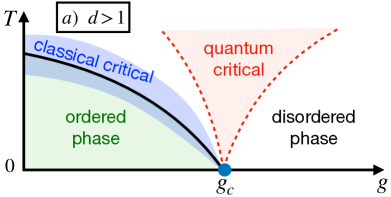
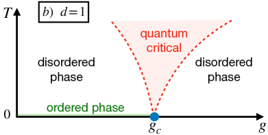
Figure 1: Sketch of the phase diagram, in the $T$-$g$ plane, for quantum Ising systems (6). Panel $a)$ is for systems in $d>1$ dimensions: at finite temperature, a line of classical transitions separates an ordered phase from a disordered phase, terminating at the QCP (for $T=0$, $g=g_{c}$). The theory of phase transitions in classical systems driven by thermal fluctuations can be applied within the shaded blue region across such transition line. Conversely, in the red region emerging from the QCP, quantum and thermal fluctuations are comparable and thus it is not possible to invoke any semiclassical description of the system behavior. Panel $b)$ shows the $1d$ case: the classical transition line disappears and the ordered phase survives only at zero temperature and for $g<g_{c}$ (with $g_{c}=1$).

In contrast, $1d$ systems such as the Ising and the XY chain, do not develop a finite-temperature transition, being always disordered for any temperature $T>0$ and value of $g$ [see Fig. 1, panel $b)$]. This is essentially related to the fact that $1d$ Ising-like systems described by the classical Gibbs ensembles do not show finite-temperature ferromagnetic transitions. However, they present a zero-temperature QCP separating quantum disordered and ordered phases.

3.1.2 Continuous quantum transitions

The critical behavior at the CQT belongs to the $(d+1)$-dimensional Ising universality class characterized by a global $\mathbb{Z}_{2}$ symmetry, associated with the $(d+1)$-dimensional quantum field theory (QFT) defined by the Lagrangian density (1) with a single-component real field [1, 37, 46, 49]. While the critical exponents $\nu$ and $\eta$ depend on $d$, the dynamic exponent $z$ is equal to

$$z=1$$ (12)

in any dimension. In particular, the critical gap $\Delta(L)$ of the 1$d$ Ising chain (6) at the CQT point $g_{c}=1$ and $h=0$ behaves as [86, 57, 109]

$$\Delta(L)_{\rm OBC}={\pi\over L}+O(L^{-2})\,,\qquad\Delta(L)_{\rm PBC}={\pi\over 2L}+O(L^{-2})\,,\qquad\Delta(L)_{\rm ABC}={3\pi\over 2L}+O(L^{-2})\,,$$ (13)

respectively for OBC, PBC, and ABC.

The CQT of quantum $1d$ systems belongs to the two-dimensional ($2d$) Ising universality class, hence its critical behavior is associated with a $2d$ conformal field theory (CFT) with central charge $c=1/2$ [116, 117]. The critical exponents assume the values

$$\nu=1\,,\quad\eta=1/4\,,\qquad{\rm for}\;\;d=1\,.$$ (14)

The structure of the scaling corrections within the $2d$ Ising universality class has been also thoroughly discussed (see, e.g., Refs. [118, 119, 120, 121, 122, 86]). The leading corrections due to irrelevant operators are generally characterized by the exponent $\omega=2$ for unitary Ising-like theories [121, 122], such as those emerging at the Ising CQTs of the XY chain. Due to the relatively large value of $\omega$, corrections from other sources may dominate for some observables, such as those arising from analytical backgrounds and/or the presence of boundaries [122, 86] (see also below). A detailed analysis of the scaling corrections at the CQT of $1d$ quantum Ising-like systems is reported in Ref. [86].

For $2d$ quantum Ising models, the critical exponents are those of the $3d$ Ising universality class, which are not known exactly, but there are very accurate estimates by various approaches, ranging from lattice techniques to statistical field theory (SFT) computations. A selection of the most recent and accurate estimates of the (classical) $3d$ Ising critical exponents is contained in Table 2, where we report the correlation-length exponent $\nu$, the exponent $\eta$ related to the space-dependence of the critical two-point function, and the scaling-correction exponent $\omega$ related to the leading irrelevant perturbation at the corresponding fixed point of the RG flow. Finally, for $3d$ quantum systems, the critical exponents assume mean-field values, i.e., $\nu=1/2$ and $\eta=0$, apart from logarithms (see, e.g., Refs. [46, 45]).

$3d$ Ising		$\nu$	$\eta$	$\omega$	Ref.year
Lattice	HT exp	0.63012(16)	0.0364(2)	0.82(4)	[123]2002
	MC	0.63020(12)	0.0372(10)	0.82(3)	[124]2003
	MC	0.63002(10)	0.03627(10)	0.832(6)	[125]2010
SFT	6-loop 3$d$ expansion	0.6304(13)	0.0335(25)	0.799(11)	[126]1998
	6-loop $\epsilon$ expansion	0.6292(5)	0.0362(6)	0.820(7)	[127]2017
	NPRG	0.63012(16)	0.0361(11)	0.832(14)	[128]2020
	CFT bootstrap	0.629971(4)	0.036298(2)	0.8297(2)	[129]2016

Table 2: Some estimates of the critical exponents of the $3d$ Ising universality class, by lattice techniques [such as high-temperature (HT) expansions [123] and Monte Carlo (MC) simulations [125, 124, 130, 131]] and statistical field theory (SFT) approaches [such as resummations of high-order SFT perturbative expansions (using 6-loop calculations within fixed-dimension [126, 132, 133, 134, 135, 136] and $\epsilon$-expansion [127, 137, 138, 139] RG schemes), nonperturbative RG (NPRG) approaches [128], and conformal field theory (CFT) bootstrap [129, 140]]. A more complete list of theoretical and experimental results can be found in Ref. [49] (at least up to 2002), however those reported here are the most accurate within the various approaches. We recall that the critical exponents controlling the asymptotic exponents of other observables, such as the magnetization, can be generally obtained from $\nu$ and $\eta$ by using scaling and hyperscaling relations (see, e.g., Refs. [46, 50]). We note that there is an overall agreement among the results obtained by the different approaches. Moreover, there is also a good agreement with experiments in various physical systems at continuous transitions such as those in liquid-vapor systems, binary systems, uniaxial magnetic systems, Coulombic systems, etc. (see, e.g., Ref. [49] for a list of experimental results).

Experimental evidence of the CQT emerging in quantum Ising-like systems has been obtained through nuclear magnetic resonance in various contexts, in particular see Refs. [141, 142, 143, 144, 145, 146].

3.1.3 First-order quantum transitions

Within the quantum Ising model of Eq. (6), the longitudinal field $h$ drives FOQTs along the line $g<g_{c}$. As already mentioned, many-body systems at FOQTs turn out to be extremely sensitive to the type of BC, whether they favor one of the phases or they are neutral, giving rise to exponential or power-law behaviors (we will return to this point later). The FOQTs of systems with BC that do not favor any of the two magnetized phases, such as PBC and OBC, are characterized by the level crossing of the two lowest states $|\!\uparrow\rangle$ and $|\!\downarrow\rangle$ for $h=0$, such that

$$\langle\uparrow\!|\hat{\sigma}_{\bm{x}}^{(1)}|\!\uparrow\rangle=m_{0}\,,\qquad\langle\downarrow\!|\hat{\sigma}_{\bm{x}}^{(1)}|\!\downarrow\rangle=-m_{0}\,,$$ (15)

with $m_{0}>0$ and independently of ${\bm{x}}$ . The degeneracy of these states is lifted by the longitudinal field $h$. Therefore $h=0$ is a FOQT point, where the (average) longitudinal magnetization $M$,

$$M\equiv L^{-d}\sum_{\bm{x}}m_{\bm{x}}\,,\qquad m_{\bm{x}}\equiv\big{\langle}\hat{\sigma}_{\bm{x}}^{(1)}\big{\rangle}\,,$$ (16)

becomes discontinuous in the infinite-volume limit. The transition separates two different phases characterized by opposite values of the magnetization $m_{0}$, i.e.,

$$\lim_{h\to 0^{\pm}}\lim_{L\to\infty}M=\pm m_{0}\,.$$ (17)

In a finite system of size $L$, the two lowest states are superpositions of magnetized states $|+\rangle$ and $|-\rangle$ such that $\langle\pm|\hat{\sigma}_{\bm{x}}^{(1)}|\pm\rangle=\pm\,m_{0}$, for all sites ${\bm{x}}$. Due to tunneling effects, the energy difference (gap) $\Delta$ of the lowest states at $h=0$ vanishes exponentially as $L$ increases [147, 55],

$$\Delta(L,h=0)\equiv E_{1}(L,h=0)-E_{0}(L,h=0)\sim e^{-cL^{d}}\,,$$ (18)

apart from powers of $L$, where $c>0$ depends on $g$. In particular, for a $1d$ quantum Ising chain with $g<1$, it is exponentially suppressed as [108, 148]

$$\Delta(L,h=0)\,= \!\!\!\!2\,(1-g^{2})\;g^{L}\,[1+O(g^{2L})] \quad\mbox{ for}\quad\mbox{OBC}\,,$$ (19a)

$$\Delta(L,h=0)\,\approx \!\!\!\!2\,\sqrt{(1-g^{2})/(\pi L)}\;g^{L}\hskip 17.07182pt \quad\mbox{ for}\quad\mbox{PBC}\,.$$ (19b)

The differences

$$\Delta_{n}(L,h)\equiv E_{n}(L,h)-E_{0}(L,h)\;,\qquad n>1\,,$$ (20)

for the higher excited states are finite for $L\to\infty$. 

The above picture based on the quasi-level crossing of the lowest states, giving rise to exponentially suppressed gaps, strongly depends on the choice of the BC. Indeed other scenarios emerge with BC forcing domain walls in the system, such as ABC and OFBC. In those two cases, the lowest-energy states are associated with domain walls (kinks), i.e., with nearest-neighbor pairs of antiparallel spins, which can be considered as one-particle states with $O(L^{-1})$ momenta. Hence, there is an infinite number of excitations with a gap of order $L^{-2}$. In particular, for $1d$ systems

$$\Delta(L,h=0)=c\,{g\over 1-g}\,{\pi^{2}\over L^{2}}+O(L^{-3})\,,$$ (21)

with $c=1$ for ABC [148] and $c=3$ for OFBC [55, 57].

3.1.4 Relation between the quantum Ising chain and the Kitaev wire

At the beginning of this section, we stated that the XY chain of Eq. (7) can be exactly mapped into a fermionic quantum wire, cf. Eq. (8), through a Jordan-Wigner transformation which maps the spin-1/2 operators into spinless fermions. However, although the bulk behaviors of the two models in the infinite-volume limit (and thus their phase diagram) are analogous, some features of finite-size systems may significantly differ. More in detail, we should stress that the BC play an important role in this mapping. As a matter of fact, the nonlocal Jordan-Wigner transformation of the XY chain (7) with PBC or ABC does not map into the fermionic model (8) with PBC or ABC. Indeed further considerations apply [106, 108], leading to a less straightforward correspondence, which also depends on the parity of the particle-number eigenvalue.

For example, the Kitaev quantum wire with ABC turns out to be gapped in both of the phases separated by the QT at $\mu_{c}=-2$. Indeed, the energy difference $\Delta$ of the two lowest states is given by

$$\Delta(L)=\sqrt{\bar{\mu}^{2}+4(2-\bar{\mu})\,[1-{\rm cos}(\pi/L)]}\,,$$ (22)

where $\bar{\mu}=\mu-\mu_{c}$, such that

$$\Delta(L)=\left\{\begin{array}[]{ll}\displaystyle|\bar{\mu}|+{\pi^{2}(2-\bar{\mu})\over|\bar{\mu}|L^{2}}+O(L^{-4})&{\rm for}\quad|\bar{\mu}|>0\,,\vspace*{2mm}\\ \displaystyle{2\pi\over L}+O(L^{-3})&{\rm for}\quad|\bar{\mu}|=0\,.\end{array}\right.$$ (23)

Therefore, the Kitaev quantum wire with ABC does not exhibit the lowest-state degeneracy of the ordered phase of the quantum Ising chain (namely, the exponential suppression of the gap with increasing $L$). The reason for such substantial difference resides in the fact that the Hilbert space of the former is restricted with respect to that of the latter, so that it is not possible to restore the competition between the two vacua belonging to the symmetric/antisymmetric sectors of the Ising model [106, 107, 86].

Note that for the simplest OBC, the XY chain can be exactly mapped into the Kitaev model with OBC. In this case, the degenerate lowest magnetized states of the XY chain for $g<1$ and $h=0$ are mapped into Majorana fermionic states localized at the boundaries [107, 149]. In finite systems, the lowest eigenstates of the Hamiltonian are combinations of the two magnetized states, corresponding to superpositions of the localized Majorana states. Indeed, in finite systems their overlap does not vanish, giving rise to the splitting $\Delta\sim e^{-L/l_{0}}$. The coherence length $l_{0}$ diverges when approaching the order-disorder transition $g\to 1^{-}$, where $l_{0}^{-1}\sim|{\rm ln}\>g|$, thus diverging as $l_{0}\sim|g-g_{c}|^{-\nu}$ with $\nu=1$ when approaching the critical point.

3.1.5 Quantum antiferromagnetic Ising chains

The quantum antiferromagnetic Ising chain, defined by the Hamiltonian (6) in $1d$ with $J<0$, shows a phase diagram analogous to that of ferromagnetic models, but with peculiar finite-size effects. Assuming $J=-1$ and $h=0$, we write its Hamiltonian as

$$\hat{H}_{\rm AIs}(g,h)=\sum_{x}\left(\hat{\sigma}^{(1)}_{x}\hat{\sigma}^{(1)}_{x+1}-g\hat{\sigma}^{(3)}_{x}\right)\,.$$ (24)

The antiferromagnetic chain (24) can be easily mapped into the ferromagnetic one (6) with $J=1$, by an appropriate transformation of the spin operators,

$$\hat{\sigma}^{(1,2)}_{x}\to(-1)^{x}\hat{\sigma}^{(1,2)}_{x}\,,\qquad\hat{\sigma}^{(3)}_{x}\to\hat{\sigma}^{(3)}_{x}\,,$$ (25)

which preserves the commutation rules. Correspondingly, we also have that the staggered magnetization $M_{\rm st}\equiv L^{-1}\sum_{x}(-1)^{x}\big{\langle}\hat{\sigma}_{x}^{(1)}\big{\rangle}$ maps into the magnetization defined in Eq. (16). Therefore the bulk properties, and the nature of the QTs, must be the same: we recover a CQT at $g_{c}=1$, and FOQTs for $g<g_{c}$ driven by a staggered external field $h_{x}=(-1)^{x}h$.

For finite-size systems of size $L$, the model (24) with OBC maps into the ferromagnetic model with OBC as well, thus they exactly share the same spectrum. However, an anomalous behavior emerges along the FOQT line when choosing PBC. Indeed, for even size $L$ the mapping (25) brings to a ferromagnetic model with PBC, thus having an exponentially suppressed energy difference of the lowest states [cf., Eq. (19b)] along the FOQT line $g<g_{c}$ and $h=0$. On the other hand, for odd $L$, the antiferromagnetic model maps into the ferromagnetic one with ABC, whose lowest states are characterized by the presence of kinks, and the gap is only power-law suppressed as in Eq. (21). This does not allow us to define a FSS limit at the FOQT of antiferromagnetic models with PBC, unless we distinguish even and odd sizes (see Sec. 5).  The frustration induced by PBC in antiferromagnetic spin chains with an odd number of sites has been also discussed in Refs. [150, 151, 152, 153].

3.2 Bose-Hubbard models

Another physically relevant system is the Bose-Hubbard (BH) model [154], which provides a realistic description of a gas of bosonic atoms loaded into an optical lattice [155]. Its Hamiltonian reads:

$$\hat{H}_{\rm BH}(U,\mu)=-t\sum_{\langle{\bm{x}},{\bm{y}}\rangle}\big{(}\hat{b}_{\bm{x}}^{\dagger}\hat{b}^{\phantom{\dagger}}_{\bm{y}}+\hat{b}_{\bm{y}}^{\dagger}\hat{b}^{\phantom{\dagger}}_{\bm{x}}\big{)}+{U\over 2}\sum_{\bm{x}}\hat{n}_{\bm{x}}(\hat{n}_{\bm{x}}-1)-\mu\sum_{\bm{x}}\hat{n}_{\bm{x}}\,,$$ (26)

where $\hat{b}_{\bm{x}}^{(\dagger)}$ annihilates (creates) a boson on site ${\bm{x}}$ of a $L^{d}$ cubic-like lattice, $\hat{n}_{\bm{x}}\equiv\hat{b}_{\bm{x}}^{\dagger}\hat{b}^{\phantom{\dagger}}_{\bm{x}}$ is the particle-density operator, the first sum runs over nearest-neighbor bonds ${\langle{\bm{x}},{\bm{y}}\rangle}$, while the two other sums run over all sites. Moreover the parameter $t$ denotes the hopping strength, $U$ the interaction strength, and $\mu$ the onsite chemical potential. In this model the total number of bosons is conserved, indeed the particle-number operator $\hat{N}\equiv\sum_{\bm{x}}\hat{n}_{\bm{x}}$ commutes with the Hamiltonian $\hat{H}_{\rm BH}$. In the following, we set $t=1$.

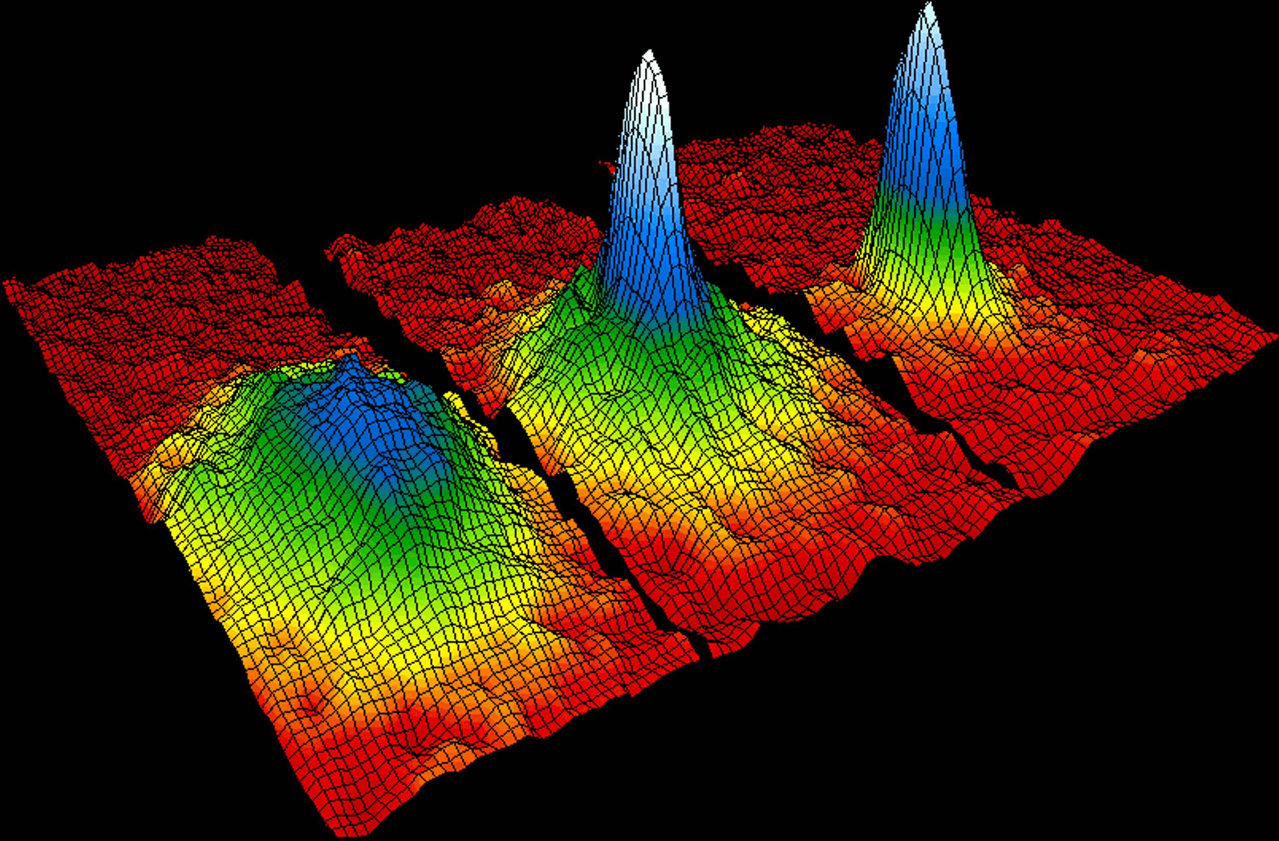
Figure 2: Three dimensional successive snapshots showing the velocity distribution data for a gas of rubidium atoms, which is progressively cooled from $200$ nK (left) down to $20$ nK (right). The coherent BEC emerges as a blue peak representing a group of atoms with the same velocity, surrounded by a field of noncondensed atoms with random velocities. Image from the National Institute of Standards and Technology (public domain).

In the infinitely repulsive (hard-core) $U\to+\infty$ limit, the particle number can only take the values $n_{\bm{x}}=0,\,1$. In such case, the BH Hamiltonian can be exactly mapped into the XX model [1]

$$\hat{H}_{\rm XX}(\mu)=-2\sum_{\langle{\bm{x}},{\bm{y}}\rangle}\left(\hat{S}^{(1)}_{\bm{x}}\hat{S}^{(1)}_{\bm{y}}+\hat{S}^{(2)}_{\bm{x}}\hat{S}^{(2)}_{\bm{y}}\right)+\mu\sum_{\bm{x}}\Big{(}\hat{S}^{(3)}_{\bm{x}}-\tfrac{1}{2}\Big{)}\,,$$ (27)

where the spin operators $\hat{S}_{\bm{x}}^{(k)}\equiv\hat{\sigma}_{\bm{x}}^{(k)}/2$ are related to the bosonic ones by: $\hat{\sigma}_{\bm{x}}^{(1)}=\hat{b}_{\bm{x}}^{\dagger}+\hat{b}^{\phantom{\dagger}}_{\bm{x}}$, $\,\hat{\sigma}^{(2)}_{\bm{x}}=i(\hat{b}_{\bm{x}}^{\dagger}-\hat{b}^{\phantom{\dagger}}_{\bm{x}})$, and $\hat{\sigma}^{(3)}_{\bm{x}}=1-2\hat{b}_{\bm{x}}^{\dagger}\hat{b}^{\phantom{\dagger}}_{\bm{x}}$. 

3.2.1 The phase diagram

The equilibrium thermodynamic behavior of the BH models is described by the partition function

$$Z={\rm Tr}\,\big{[}e^{-\beta H_{\rm BH}(U,\,\mu)}\big{]}\,,\qquad\quad\beta\equiv 1/T\,.$$ (28)

They show various phases depending on the temperature $T$, the chemical potential $\mu$, and in particular on the spatial dimension $d$.

The low-temperature behavior of $3d$ bosonic gases is characterized by the Bose-Einstein condensation (BEC) phenomenon, below a finite temperature $T_{c}$. The BEC phase transition at $T_{c}$ separates the high-temperature normal phase and the low-temperature superfluid BEC phase. This is characterized by the accumulation of a macroscopic number of atoms in a single quantum state, giving rise to a phase-coherent condensate, as shown in Fig. 2. The phase coherence properties of the BEC phase have been observed in a number of spectacular experiments with ultracold gases (see, e.g., Refs. [156, 157, 158, 159, 160, 161, 162, 163, 164, 165, 166]). Several theoretical and experimental studies have also investigated the critical properties at the BEC transition, when the condensate forms (see, e.g., Refs. [167, 168, 169, 170, 171, 172, 173, 174, 175, 176, 177, 178, 179, 180, 181, 182, 183, 184, 185, 186, 187, 188, 189, 190, 191, 192, 193, 194, 195]).

Figure 3: Sketch of the phase diagram, in the $T$-$\mu$ plane, for the BH model in the hard-core $U\to\infty$ limit (27). We adopt units of the hopping parameter $t$. Panel $a$) shows the $3d$ case: The BEC phase is restricted to a finite region for $|\mu|\leq 6$. It is bounded by a BEC transition line $T_{c}(\mu)$, which satisfies $T_{c}(\mu)=T_{c}(-\mu)$ due to a particle-hole symmetry. Its maximum occurs at $\mu=0$, where [186, 190] $T_{c}(\mu=0)=2.01599(5)$; we also know that [185] $T_{c}(\mu=\pm 4)=1.4820(2)$. At $T=0$ two further quantum phases exist, i.e., the vacuum ($\mu<-6$) and the incompressible $n=1$ Mott insulator phase ($\mu>6$). Panel $b$) shows the $2d$ case: The normal and superfluid QLRO phases are separated by a finite-temperature BKT transition line, which satisfies $T_{\rm BKT}(\mu)=T_{\rm BKT}(-\mu)$ due to a particle-hole symmetry. Its maximum occurs at $\mu=0$, where [196] $T_{\rm BKT}(\mu=0)=0.6877(2)$. The superfluid QLRO phase is restricted to a finite region for $|\mu|\leq 4$.

The phase diagram of a $3d$ BH model, and its critical behavior, have been deeply investigated (see, e.g., Refs. [154, 169, 197, 184, 185, 186, 190]). The $T$-$\mu$ phase diagram presents a finite-temperature BEC transition line, as shown in Fig. 3, panel $a$), for the hard-core $U\to\infty$ limit, where the occupation site number is limited to the cases $n_{\bm{x}}=0,\,1$. The condensate wave function provides the complex order parameter of the BEC transition, whose critical behavior belongs to the $3d$ U(1)-symmetric $XY$ universality class . This implies that the length scale $\xi$ of the critical modes diverges at $T_{c}$ as

$$\xi\sim(T-T_{c})^{-\nu},\qquad\nu\approx 0.6717\,.$$ (29)

A selection of the most recent and accurate estimates of the $3d$ $XY$ critical exponents is reported in Table 3. The power law (29) has been accurately verified by numerical studies at the BEC phase transition (see, e.g., Refs. [184, 185, 186, 190]). The BEC phase extends below the BEC transition line. In particular, in the hard-core limit $U\to\infty$ and for $\mu=0$ (corresponding to half filling), the BEC transition occurs at $T_{c}=2.01599(5)$ [186, 190].

$3d$ $XY$		$\nu$	$\eta$	$\omega$	Ref.year
Lattice	HT+MC	0.6717(1)	0.0381(2)	0.785(20)	[198]2006
	MC	0.6717(3)			[199]2006
	MC	0.67169(7)	0.03810(8)	0.789(4)	[200]2019
SFT	6-loop 3$d$ expansion	0.6703(15)	0.035(3)	0.789(11)	[126]1998
	6-loop $\epsilon$ expansion	0.6690(10)	0.0380(6)	0.804(3)	[127]2017
	NPRG	0.6716(6)	0.0380(13)	0.791(8)	[128]2020
	CFT bootstrap	0.67175(10)	0.038176(44)	0.794(8)	[201]2020
Experiment	4He	0.6709(1)			[202, 203, 204]1996

Table 3: Some estimates of the universal critical exponents for the $3d$ $XY$ universality class. We report the correlation-length exponent $\nu$, the order-parameter exponent $\eta$, and the exponent $\omega$ associated with the leading scaling corrections. They were obtained from the analysis of HT expansions supplemented by MC simulations [198], MC simulations [199, 200], QFT approaches based on the resummation of high-order series [126, 127], nonperturbative RG (NPRG) approaches [128], the conformal-bootstrap approach [201], and experiments of the ⁴He superfluid transition in microgravity environment [204, 202] (whose estimate of $\nu$ is obtained from the measurement of the specific-heat exponent $\alpha=-0.0127(3)$ and the hyperscaling relation $d\nu=2-\alpha$). See Ref. [49] for a more complete list of theoretical and experimental results. As already noted in the literature, the experimental estimate of $\nu$, reported in the table, is not consistent with the most accurate theoretical estimates, likely because its error is somehow too optimistic. In this respect, one should take into account the difficulty of extracting the specific-heat exponent $\alpha$ from the temperature dependence of the specific heat close to $T_{c}$, due to the fact that it is negative ($\alpha\approx-0.0150$). Thus, it is not associated with the leading behavior of the specific heat, which is dominated by a nonuniversal constant term [202, 49, 198], i.e., $C\approx a+b|T-T_{c}|^{-\alpha}+\ldots$, and for small $|\alpha|$ the first two leading terms are hardly distinguishable.

On the other hand, $2d$ bosonic gases do not display BEC phases, because a nonvanishing order parameter cannot appear in $2d$ (or quasi-$2d$) systems with a global U(1) symmetry [205, 206]. However, $2d$ (or quasi-$2d$) systems with a global U(1) symmetry may undergo a finite-temperature transition described by the BKT theory [53, 52, 54, 207, 208, 209]. The BKT transition separates a high-temperature normal phase and a low-temperature phase characterized by quasi-long-range order (QLRO), where correlations decay algebraically at large distances, without the emergence of a nonvanishing order parameter [205, 206]. When approaching the BKT transition point $T_{\rm BKT}$ from the high-temperature normal phase, these systems develop an exponentially divergent correlation length

$$\xi\sim\exp\left({c/\sqrt{\tau}}\right),\qquad\tau\equiv T/T_{\rm BKT}-1\,,$$ (30)

where $c$ is a nonuniversal constant. Consistently with the above picture, the $2d$ BH system undergoes a BKT transition. Figure 3, panel $b$), shows a sketch of its phase diagram in the hard-core $U\to\infty$ limit. The finite-temperature BKT transition of BH models has been numerically investigated by several studies (see, e.g., Refs. [210, 211, 212, 213, 184, 196, 193]). In particular, $T_{\rm BKT}=0.6877(2)$ for $U\to\infty$ and for $\mu=0$ [196]. Below the critical temperature $T_{\rm BKT}$, $2d$ BH systems show a QLRO phase, where the phase-coherence correlations decay algebraically. Experimental evidence of BKT transitions has been also reported for quasi-$2d$ trapped atomic gases [214, 215, 216, 217, 218, 219, 220].

3.2.2 Zero-temperature quantum transitions

The zero-temperature phase diagram can be investigated using mean-field approaches (see, e.g., Refs. [154, 1]). In the absence of the hopping term, a uniform chemical potential fixes the occupation site number to its integer part plus one. Once $\mu$ is fixed, the BH Hamiltonian (26) is characterized by the competition between the onsite repulsion $U$ and the nearest-neighbor hopping $t$. For $U\gg t$, strong local interactions force bosons to be localized into a gapped Mott insulator (MI) phase. In the opposite $U\ll t$ limit, bosons are delocalized in a gapless superfluid phase. The onset of these two phases has been observed in a clearcut way, through experiments with ultracold atoms trapped in optical lattices [221, 222]. A direct transition between the two phases occurs at a given critical value of the ratio $t/U$, which depends on the chemical potential, in such a way that a lobe structure arises [154] in the $\mu$-$(1/U)$ plane, as sketched in Fig. 4: the higher the Mott particle number, the smaller the lobe in the phase diagram. The system dimensionality can affect the form and the size of the lobes, but not this general structure .

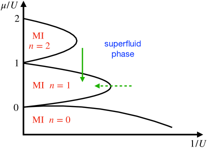
Figure 4: Sketch of the zero-temperature mean-field phase diagram, in the $\mu$-$(1/U)$ plane, of the BH model. We fix $t=1$. The lobes, surrounded by the superfluid region, correspond to MI islands with integer filling factor $n$. The green lines denote two types of parameters variations driving CQTs from a superfluid to a MI phase. The CQT along the vertical line, corresponding to varying the chemical potential, belongs to the nonrelativistic U(1)-symmetric bosonic QFT universality class. The CQT along the dashed line, at fixed integer density, belongs to the relativistic U(1)-symmetric bosonic QFT universality class.

Focusing on the hard-core limit, or equivalently on the XX model (27), one can observe the emergence of three phases associated with the ground-state properties [1]: the vacuum ($\mu<-2d$), the superfluid ($|\mu|<2d$), and the $n=1$ MI phase ($\mu>2d$). The vacuum-to-superfluid transition at $\mu_{\textrm{v-s}}=-2d$  and the $n=1$ superfluid-to-MI transition at $\mu_{\textrm{s-MI}}=2d$, when driven by the chemical potential (as in the vertical green line in Fig. 4), belong to the universality class associated with a nonrelativistic U(1)-symmetric bosonic field theory [154, 1]. Its partition function is given by

$$Z=\int[{\rm D}\phi]\,\exp\!\bigg{[}-\int_{0}^{1/T}{\rm d}t\>{\rm d}^{d}x\,\Big{(}\phi^{*}\partial_{t}\phi+\tfrac{1}{2m}|\nabla\phi|^{2}+r|\phi|^{2}+u|\phi|^{4}\Big{)}\bigg{]}\,,$$ (31)

where $r\sim\mu-\mu_{c}$. The upper critical dimension of this bosonic field theory is $d=2$. Thus its critical behavior is mean-field for $d>2$. For $d=2$ the field theory is essentially free (apart from logarithmic corrections), thus the dynamic critical exponent is $z=2$, while the RG dimension of the relevant parameter $r=\mu-\mu_{c}$ is $y_{r}=2$. In $d=1$ the theory turns out to be equivalent to a quadratic field theory of nonrelativistic spinless fermions [1], from which one infers the RG exponents $z=2$ and $y_{r}=2$.

The special transitions at fixed integer density (i.e., fixed $\mu$) (as in the horizontal dashed green line in Fig. 4) belong to a different universality class, described by a relativistic U(1)-symmetric bosonic field theory [154], given by the $(d+1)$-dimensional O(2)-symmetric $\Phi^{4}$ Lagrangian (1) with $N=2$. Therefore, the dynamic exponent is $z=1$, and $y_{r}=1/\nu$ where $\nu$ is the correlation length exponent of the $(d+1)$-$XY$ universality class. Thus $\nu=1/2$ for $d=3$ (i.e., mean-field behavior apart from logarithms), $\nu\approx 0.6717$ for $d=2$ (see Table 3), and an exponential behavior formally corresponding to $\nu=\infty$ for the BKT transition [53, 209] at $d=1$.

3.2.3 Bose-Hubbard model with extended interactions

The physics of the BH model can be considerably enriched by extending the range of interactions beyond the onsite limit. In particular, one can construct the following Hamiltonian for the extended BH model:

$$\hat{H}_{\rm EBH}(V,U,\mu)=\hat{H}_{\rm BH}(U,\mu)+V\sum_{{\bm{x}}\neq{\bm{y}}}\frac{1}{|\bm{x}-\bm{y}|^{3}}\,\hat{n}_{\bm{x}}\hat{n}_{\bm{y}}\,,$$ (32)

where $V$ denotes the nonlocal two-body interaction strength. From a physical point of view, this model faithfully describes dipolar bosons confined in optical lattices, in which repulsive interactions have a long-range character and are typically decaying with the distance as $r^{-3}$ [227, 228].

The above model has been studied in some detail in the $1d$ case, showing that it may stabilize an insulating phase, named the bosonic Haldane insulator (HI) phase. This phase is of topological kind, since it breaks a hidden $\mathbb{Z}_{2}$ symmetry related to a string order parameter. The latter is characterized by a non-trivial ordering of the fluctuations that appear in alternating order separated by strings of equally populated sites of arbitrary length, being described by the correlator [229, 230]

$$R_{\rm string}(r)=\big{\langle}\delta\hat{n}_{x}\,e^{i\pi\sum_{k=x}^{y}\delta\hat{n}_{k}}\,\delta\hat{n}_{y}\big{\rangle}\,,$$ (33)

where $\delta\hat{n}_{x}=\hat{n}_{x}-\bar{n}$ denotes the boson number fluctuations from the average filling $\bar{n}$.

When varying $U$ and $V$, the phase diagram of the extended BH model supports a wealth of different phases (see Ref. [231] for a review): at commensurate fillings, the presence of interactions between distant sites may lead to a density-modulated insulating phase with staggered order, also named density wave. In $1d$, the topological HI phase emerges in between the MI and the density wave, as verified through numerical density-matrix renormalization group (DMRG) calculations [229, 230, 232]. For incommensurate fillings, other peculiar features appear, such as the supersolid phase and phase-separation regions. It is worth pointing out that the MI and HI phases can be adiabatically connected by opening a gap at the critical point separating them, through an additional Hamiltonian term which breaks the inversion symmetry of the system (e.g., via a correlated tight-binding hopping). By suitably tuning the various Hamiltonian parameters, it is thus possible to adiabatically encircle the MI-HI critical point and therefore to enable quantized transport through adiabatic pumping [233, 234].

3.3 Quantum rotor and Heisenberg spin models

Another paradigmatic model is the so-called quantum rotor model, for which the basic orientation operator is a $N$-component unit vector $\hat{\bm{n}}_{\bm{x}}$, such that $\hat{\bm{n}}_{\bm{x}}\cdot\hat{\bm{n}}_{\bm{x}}=1$, with a corresponding momentum $\hat{\bm{p}}_{\bm{x}}$, such that $\big{[}\hat{n}^{a}_{\bm{x}},\hat{p}^{b}_{\bm{y}}\big{]}=i\delta_{{\bm{x}}{\bm{y}}}\delta^{ab}$. Introducing the angular momentum operator $\hat{L}_{\bm{x}}^{ab}\equiv\hat{n}^{a}_{\bm{x}}\,\hat{p}^{b}_{\bm{x}}-\hat{n}^{b}_{\bm{x}}\,\hat{p}^{a}_{\bm{x}}$, and in particular $\hat{L}_{\bm{x}}^{c}={1\over 2}\epsilon^{abc}\hat{L}^{ab}_{\bm{x}}$ for $N=3$, we can write the corresponding $d$-dimensional Hamiltonian as [1]

$$\hat{H}_{\rm rot}=-J\sum_{\langle{\bm{x}},{\bm{y}}\rangle}\hat{\bm{n}}_{\bm{x}}\cdot\hat{\bm{n}}_{\bm{y}}+g\sum_{\bm{x}}\hat{\bm{L}}_{\bm{x}}^{2}\,,$$ (34)

where the first sum is over all bonds connecting nearest-neighbor sites $\langle{\bm{x}},{\bm{y}}\rangle$ of a $L^{d}$ cubic-like lattice, while the other sum is over all sites. We fix $J=1$. For $d\geq 2$ the system shows a quantum paramagnet phase for large values of $g$, and a magnetized phase for small values of $g$, similarly to quantum Ising systems (6). A CQT separates the two phases at a finite coupling value $g_{c}$, which is associated with the symmetry-breaking pattern O($N$) $\to$ O($N-1$). For $d=1$ and $N\geq 3$, the rotor model only features a quantum paramagnetic phase, i.e., $g_{c}=0$ formally.

The quantum criticality of these models is thoroughly discussed in Ref. [1]. The corresponding QFT is provided by a $(d+1)$-dimensional $\Phi^{4}$ field theory (1) with $N=3$. The cases for $N=3$ are also referred to as Heisenberg spin models. Some accurate results for the universal critical exponents of the $3d$ Heisenberg universality class, providing the asymptotic behavior for $2d$ QTs, are reported in Table 4. Results for $N>3$ universality classes can be found in Refs. [49, 235] and large-$N$ computations in Ref. [236]. Phase transitions breaking the O($N$) symmetry are not expected in 1$d$ quantum Heisenberg spin models, since the corresponding 2$d$ classical models do not undergo phase transitions, indeed they only show disordered phases with an asymptotic critical behavior in the zero-temperature limit, characterized by an exponential increase of the correlation length, as $\xi\sim e^{c/T}$ (see, e.g., Refs. [46, 49]).

$3d$ Heisenberg		$\nu$	$\eta$	$\omega$	Ref.year
Lattice	HT+MC	0.7112(5)	0.0375(5)		[237]2002
	HT+MC	0.7117(5)	0.0378(5)		[235]2011
	HT+MC	0.7116(2)	0.0378(3)		[238]2020
	MC	0.71164(10)	0.03784(5)	0.759(2)	[238]2020
SFT	6-loop 3$d$ expansion	0.7073(35)	0.0355(25)	0.782(13)	[126]1998
	6-loop $\epsilon$ expansion	0.7059(20)	0.03663(12)	0.795(7)	[127]2017
	NPRG	0.7114(9)	0.0376(13)	0.769(11)	[128]2020
	CFT bootstrap	0.7117(4)	0.03787(13)		[239]2020

Table 4: Some estimates of the universal critical exponents for the $3d$ Heisenberg universality class. We report the correlation-length exponent $\nu$, the order-parameter exponent $\eta$, and the exponent $\omega$ associated with the leading scaling corrections. They were obtained from the analysis of high-order HT expansions supplemented by MC simulations [237, 235, 238], MC simulations [238] QFT approaches based on the resummation of high-order series [126, 127], nonperturbative RG (NPRG) approaches [128], the conformal-bootstrap approach [239]. See Refs. [49, 238] for a more complete list of theoretical and experimental results.

The $N=3$ quantum rotors have some connections with certain dimerized antiferromagnetic systems of Heisenberg spins $\hat{\bm{S}}_{\bm{x}}\equiv\big{(}\hat{S}_{\bm{x}}^{(1)},\hat{S}_{\bm{x}}^{(2)},\hat{S}_{\bm{x}}^{(3)}\big{)}$ located at each lattice site, belonging to the spin-$S$ representation. As argued in Ref. [1], under some conditions, quantum rotor models provide the low-energy properties of a class of quantum antiferromagnets. Heisenberg quantum antiferromagnets [240, 241] are generally defined as sum of terms associated with the bonds of the lattice,

$$\hat{H}_{\rm He}=\sum_{\langle{\bm{x}},{\bm{y}}\rangle}J_{{\bm{x}},{\bm{y}}}\,\hat{\bm{S}}_{\bm{x}}\cdot\hat{\bm{S}}_{\bm{y}}\,.$$ (35)

Various behaviors may arise from different lattice geometries and corresponding bond couplings $J_{{\bm{x}},{\bm{y}}}$.

The phase diagram and critical behaviors of quantum Heisenberg antiferromagnets with homogeneous bonds $J_{{\bm{x}},{\bm{y}}}=J>0$ have been largely discussed in the literature. The quantum fluctuations do not allow long-range order in $1d$ models: they remain always gapped for integer $S$ or may become critical for half odd-integer S [242, 243, 244, 245]. On a $2d$ square lattice, the ground state is ordered for all $S$ [246, 247, 248, 249]. For $T>0$, the order is destroyed by thermal fluctuations [205]. However, it develops an exponential critical behavior in the $T\to 0$ limit, described by the asymptotically free $2d$ O(3) nonlinear $\sigma$ model (see, e.g., Refs. [250, 251, 252, 253, 254, 255, 49]). The ground state is ordered also in $3d$ homogeneous Heisenberg antiferromagnets. However, the ordered phase generally persists at low temperature, up to a finite-temperature transition to a disordered phase, belonging to the $3d$ Heisenberg universality class characterized by the symmetry-breaking pattern O(3) $\to$ O(2) (see, e.g., Refs. [256, 257] and references therein).

QCPs separating quantum ordered and disordered phases can be observed when the bond couplings are not homogeneous, such as the $S=1/2$ Heisenberg antiferromagnet on an inhomogeneous square lattice with tunable interaction between spins belonging to different plaquettes [258], double-layer Heisenberg antiferromagnets [259], etc. (see also [1] for a more detailed discussion).

We also mention another interesting issue related to the phase transitions between Néel and VBS phases in Heisenberg antiferromagnets [97]. Since both phases break a global Hamiltonian symmetry (spin rotation and lattice rotation, respectively), and two symmetries are unrelated to each other, the conventional LGW theory of phase transitions implies that such phases must be separated by a FOQT. However, arguments in favor of a continuous phase transition have been put forward [252, 260, 98, 99, 1], based on the concept of deconfined criticality. Indeed, the Néel-to-VBS transition in $2d$ antiferromagnetic SU(2) quantum systems represent paradigmatic models for deconfined criticality, arising from the emergence of a U(1) gauge field, see also Refs. [261, 262, 263, 264, 265, 266, 267, 268, 269, 270, 271, 272, 273, 274, 275, 276, 277]. The corresponding theory at the transition is supposed to be the $3d$ Abelian-Higgs (scalar electrodynamics) theory [46] characterized by a U(1) gauge symmetry. In particular, the relevant model is expected to be the lattice Abelian-Higgs model with two-component complex scalar fields and noncompact gauge fields (in which there are no monopoles). This is of interest in several condensed-matter physics applications, since the presence of Berry phases in the quantum setting gives rise to the suppression of monopoles  (see, e.g., Ref. [269] and references therein). Note that noncompact gauge fields give rise to important differences with respect to lattice Abelian-Higgs models with compact gauge fields [279]. Theoretical and numerical investigations of classical and quantum transitions, which are expected to be in the same universality class as those occurring in noncompact scalar electrodynamics with two-component scalar fields, have provided evidence of weakly first-order or continuous transitions belonging to a new universality class (see, e.g., Refs. [98, 280, 263, 264, 265, 281, 282, 283, 284, 285, 286, 287, 288, 266, 289, 290, 271, 272, 273, 291, 270, 274, 292, 293, 275, 294, 295, 296, 297]).

4 Equilibrium scaling behavior at continuous quantum transitions

In this section we report an overview of the equilibrium scaling properties expected at generic CQTs, as inferred by the RG theory of critical phenomena specialized to QTs, i.e., taking into account the peculiar features that distinguish QTs from the classical transitions driven by thermal fluctuations. We present a detailed analysis of the RG scaling ansatz in the thermodynamic limit and in the FSS limit. The asymptotic quantum critical behaviors, and the scaling corrections characterizing the approach to the leading laws, have been thoroughly checked in various analytical and numerical studies (see in particular Ref. [86], containing a detailed study for the quantum XY chains).

4.1 Quantum-to-classical mapping

Several fundamental ideas of the RG theory of critical phenomena find their origins in the seminal works on classical systems by Kadanoff, Fisher, Wilson, among the others (see, e.g., Refs. [298, 38, 39, 40, 41, 42, 64, 44, 299, 300, 115, 112, 114, 48, 46, 45, 116, 49, 47]). Their extension to quantum systems is based on the quantum-to-classical mapping, which allows one to map the quantum system on a spatial volume $V_{s}$ onto a classical one defined in a box of volume $V_{c}=V_{s}\times L_{T}$, with $L_{T}=1/T$ (using the appropriate units) [2, 1, 86]. In fact, under the quantum-to-classical mapping, the inverse temperature corresponds to the system size in an imaginary time direction. The BC along the imaginary time are periodic or antiperiodic, respectively for bosonic and fermionic excitations. Thus, the temperature scaling at a QCP in $d$ dimensions is analogous to FSS in a corresponding $(d+1)$-dimensional classical system.

Before presenting the main ideas of the RG scaling theory at CQTs, we would like to further comment on the quantum-to-classical mapping as guiding approach. It is important to stress that such mapping does not generally lead to standard classical isotropic systems in thermal equilibrium. Indeed, while it is true that a quantum system can be mapped onto a classical one, the corresponding classical systems are generally anisotropic. In some cases, when the dynamic exponent is $z=1$ like Ising CQTs, the anisotropy is weak, as in the classical Ising model with direction-dependent couplings. In these cases, a straightforward rescaling of the imaginary time allows one to recover space-time rotationally invariant (relativistic) $\Phi^{4}$ theories such as those reported in Eq. (1). There are also interesting cases in which $z\not=1$, such as the superfluid-to-vacuum and Mott transitions of lattice particle systems described by the Hubbard and BH models, which have $z=2$ when they are driven by the chemical potential (see Sec. 3.2). For CQTs with $z\neq 1$, the anisotropy is strong, i.e., correlations have different exponents in the spatial and thermal directions. Indeed, in the case of quantum systems of size $L$, under a RG rescaling by a factor $b$ such that $\xi\to\xi/b$ and $L\to L/b$, the additional spatial dimension related to the temperature must rescale differently, as $L_{T}\to L_{T}/b^{z}$.  However, scaling and FSS is also established for classical transitions with such anisotropies [301].  Therefore, the classical FSS framework [42, 303, 112, 114, 304, 49] can be generally extended to systems at CQTs [2, 86].

We also mention another problem of the quantum-to-classical mapping: in some cases, the corresponding classical system has complex-valued Boltzmann weights, which can be hardly studied in the classical framework. The above considerations suggest that, to achieve a satisfactory understanding of the quantum dynamics in many-body systems, in particular when addressing issues related to the real-time out-of-equilibrium dynamics, a discussion of the specific problems related to the quantum nature of the phenomena is often required [1], in addition to approaches based on the quantum-to-classical mapping.

4.2 Scaling law of the free energy in the thermodynamic limit

According to the RG theory of critical phenomena, the Gibbs free energy obeys a general scaling law. Indeed, we can write it in terms of the nonlinear scaling fields associated with the RG eigenoperators at the fixed point of the RG flow [42, 49]. Guided by the quantum-to-classical mapping and the RG theory of critical phenomena, analogous scaling laws are assumed at CQTs [2, 86]. Therefore, close to a CQT the Gibbs free-energy density

$$F\equiv-{T\over V}\ln Z\,,\qquad Z={\rm Tr}\,\big{[}e^{-\hat{H}/T}\big{]}\,,$$ (36)

in the thermodynamic infinite-volume limit can be written in terms of scaling fields [42], such as [86]

$$F(T,r,h)=F_{\rm reg}(r,h^{2})+F_{\rm sing}\big{(}u_{t},u_{r},u_{h},\{v_{i}\}\big{)}\,.$$ (37)

Here $F_{\rm reg}$ is a nonuniversal function, which is analytic at the critical point and must be even with respect to the parameter $h$ related to the odd perturbation; it is also generally assumed not to depend on $T$ [86].  The other contribution, $F_{\rm sing}$, bears the nonanalyticity of the critical behavior and its universal features. The arguments of $F_{\rm sing}$ are the so-called nonlinear scaling fields [42]. They are analytic nonlinear functions of the model parameters, associated with the eigenoperators that diagonalize the RG flow close to the RG fixed point. The scaling fields $u_{r}$ and $u_{h}$ are the relevant fields related to the model parameters $r$ and $h$. The scaling field $u_{t}$ associated with the temperature, $u_{t}\sim T$, is also relevant and has a RG dimension $y_{t}=z$. Beside the relevant scaling fields, there is also an infinite number of irrelevant scaling fields $\{v_{i}\}$ with negative RG dimensions $y_{i}$, which are responsible for the scaling corrections to the asymptotic critical behavior in the infinite-volume limit. Using the standard notation (see, e.g., Ref. [49]) and assuming that they are ordered so that $|y_{1}|\leq|y_{2}|\leq\ldots$, we set

$$\omega=-y_{1}\,.$$ (38)

In general, the nonlinear scaling fields depend on the control parameters $r$, $h$, and $T$. However $u_{r}$, $u_{h}$, and $\{v_{i}\}$ are conjectured not to depend on the temperature and the system size [86].  Taking into account the assumed ${\mathbb{Z}}_{2}$ symmetry and the respectively even and odd properties of $r$ and $h$, close to the critical point the relevant scaling fields $u_{r}$ and $u_{h}$ can be generally expanded as

$$u_{r}=r+c_{r}r^{2}+O(r^{3},h^{2}r)\,,\qquad\qquad u_{h}=h+c_{h}rh+O(h^{3},r^{2}h)\,,$$ (39)

where $c_{r}$ and $c_{h}$ are nonuniversal constants. As for the irrelevant scaling fields, they are usually nonvanishing at the critical point. The thermal scaling field $u_{t}$ is expected to behave as [86]

$$u_{t}=s(r,h)\,T\,,\qquad\qquad s(r,h)=s_{0}+s_{r}r+O(r^{2},h^{2})\,,$$ (40)

where $s(r,h)$ is an appropriate nonuniversal function, while $s_{0}$ and $s_{r}$ are constant (see also Sec. 4.4.1, where this expression of $u_{t}$ is argued in the FSS context).

The singular part of the free energy (37) is expected to satisfy the homogeneous scaling law

$$F_{\rm sing}\big{(}u_{t},u_{r},u_{h},\{v_{i}\}\big{)}=b^{-(d+z)}\,F_{\rm sing}\big{(}b^{z}u_{t},b^{y_{r}}u_{r},b^{y_{h}}u_{h},\{b^{y_{i}}v_{i}\}\big{)}\,,$$ (41)

where $b$ is an arbitrary scale factor, and the critical limit is obtained in the large-$b$ limit. To obtain more explicit scaling relations, one can fix the arbitrariness of the scale parameter $b$, such as

$$b=u_{t}^{-1/z}\,,$$ (42)

which diverges in the critical limit $u_{t}\to 0$. The following asymptotic behavior of the free-energy density emerges:

$$F=F_{\rm reg}(r,h^{2})+u_{t}^{d/z+1}\,{\cal F}\big{(}u_{t}^{-y_{r}/z}u_{r},u_{t}^{-y_{h}/z}u_{h},\big{\{}{u_{t}^{-y_{i}/z}v_{i}}\big{\}}\big{)}\,.$$ (43)

For $h=0$ and $u_{t}\to 0$, since $y_{i}<0$ and $y_{1}=-\omega$, we can expand it as

$$F\approx F_{\rm reg}(r,0)+u_{t}^{d/z+1}{\cal F}_{0}\big{(}u_{t}^{-y_{r}/z}u_{r}\big{)}+u_{t}^{d/z+1+\omega/z}{\cal F}_{\omega}\big{(}u_{t}^{-y_{r}/z}u_{r}\big{)}+\ldots\,,$$ (44)

where ${\cal F}_{0}$ and ${\cal F}_{\omega}$ are scaling functions. Note that, to eventually obtain the scaling relations in terms of the external parameters $r,h$ and $T$ controlling the critical behavior, one needs to expand the scaling fields, cf. Eq. (39), whose subleading terms gives rise to analytical scaling corrections. Therefore, the scaling relation (44) predicts that the free-energy density approaches the asymptotic behavior given by the first term, with nonanalytic scaling corrections due to the irrelevant RG perturbations and analytic contributions which are due to the regular background associated with $F_{\rm reg}$ and to the expansions of the nonlinear scaling fields in terms of the Hamiltonian parameters.

Differentiating the Gibbs free energy, one can straightforwardly derive analogous scaling ansatze for the energy density

$$E(T,r,0)\equiv F-T{\partial F\over\partial T}\approx E_{\rm reg}(r,0)+T^{d/z+1}\,\big{[}{\cal E}_{0}\big{(}T^{-y_{r}/z}r\big{)}+T^{\omega/z}{\cal E}_{\omega}\big{(}T^{-y_{r}/z}r\big{)}+\ldots\big{]}\,,$$ (45)

and the specific heat

$$C_{V}\equiv{\partial E\over\partial T}\approx T^{d/z}\,\big{[}{\cal C}_{0}\big{(}T^{-y_{r}/z}r\big{)}+T^{\omega/z}{\cal C}_{\omega}\big{(}T^{-y_{r}/z}r\big{)}+\ldots\big{]}\,.$$ (46)

Notice that the specific heat does not get contributions from the regular part of the free energy, since $F_{\rm reg}$, thus $E_{\rm reg}$, is assumed to be independent of $T$. At the critical point $r=0$, Eq. (46) predicts

$$C_{V}\sim T^{d/z}\big{[}1+O(T^{\omega/z})\big{]}\,.$$ (47)

4.3 Universality of the scaling functions

As already mentioned, the critical exponents characterizing the power laws at continuous transitions are universal, i.e., they are shared by all systems belonging to the given universality class, defined by a few global features. The universality extends to scaling functions such as $\cal F$, related to the singular part of the free energy, cf. Eq. (53), and more generally to the scaling functions associated with other different quantities, which include the derivative of the free energy, the correlation functions (see also below), etc.

Since scaling fields are arbitrarily normalized, universality holds apart from a normalization of each argument and an overall constant. Therefore, given two different models, if ${\cal A}_{1}$ and ${\cal A}_{2}$ are their scaling functions associated with a generic observable, they are generally related as

$${\cal A}_{1}\big{(}x_{1},x_{2},\ldots)=c_{0}\,{\cal A}_{2}\big{(}c_{1}x_{1},c_{2}x_{2},\ldots\big{)}\,,$$ (48)

where $c_{i}$ are nonuniversal constants. The above considerations apply to generic scaling functions including those related to the scaling corrections, extending also to the cases they allow for further arguments, such as the system size and the spatial coordinates for the correlation functions.

4.4 Equilibrium finite-size scaling

The RG scaling theory developed in Sec. 4.2 holds in the thermodynamic limit, that is expected to be well defined for any $r\neq 0$ or $h\neq 0$, for which the correlation length $\xi$ is finite. Nonetheless, for practical purposes, both experimental and numerical, one typically has to face with systems of finite length. Such situations can be framed within the FSS framework, whose scaling relations are obtained by also allowing for the dependence on the size $L$.

Finite-size effects in critical phenomena have been the object of theoretical studies for a long time [110, 111, 112, 114, 115, 49]. FSS describes the critical behavior around a critical point, when the correlation length $\xi$ of the critical modes becomes comparable to the size $L$ of the system. For large sizes, this regime presents universal features, shared by all systems whose transition belongs to the same universality class. Although originally formulated in the classical framework, FSS also holds at zero-temperature QTs [2, 86] in which the critical behavior is driven by quantum fluctuations. Indeed, the RG approach [42, 112, 114, 49] to FSS at classical finite-temperature transitions (generally driven by thermal fluctuations) can be extended to QTs. This allows us to characterize the asymptotic FSS behavior at QTs, and also the nature of the corrections in systems of large, but finite, size.

The FSS limit is essentially defined as the large-$L$ limit, keeping the ratio $\xi/L$ fixed, where $\xi$ is a generic length scale of the system, which diverges at the critical point. The FSS limit definitely differs from the thermodynamic limit, which is generally obtained by taking the large-$L$ limit, keeping $\xi$ fixed; then the infinite-volume critical behavior is developed when $\xi\to\infty$. However, assuming an asymptotic matching of the FSS and the thermodynamic limit, one may straightforwardly derive the infinite-volume scaling behaviors from FSS, by taking the $\xi/L\to 0$ limit of the FSS ansatz.

The FSS approach is one of the most effective techniques for the numerical determination of the critical quantities. While infinite-volume methods require that the condition $\xi\ll L$ is satisfied, FSS applies to the less demanding regime $\xi\sim L$. More precisely, the FSS theory provides the asymptotic scaling behavior when both $L,\xi\to\infty$, keeping their ratio $\xi/L$ fixed. However, the knowledge of the asymptotic behavior may not be enough to estimate the critical parameters, because data are generally available for limited ranges of parameter values and system sizes, which are often relatively small. Under these circumstances, the asymptotic FSS predictions are affected by sizable scaling corrections. Thus, reliably accurate estimates of the critical parameters need a robust control of the corrections to the asymptotic behavior. This is also important for a conclusive identification of the universality class of the quantum critical behavior when it is a priori uncertain. Moreover, an understanding of the finite-size effects is relevant for the experiments, when relatively small systems are considered (see, e.g., Ref. [305]), or in particle systems trapped by external (usually harmonic) forces, as in cold-atom setups (see, e.g., Refs. [156, 157, 170, 166, 173, 306]).

4.4.1 The free-energy density

Within the FSS framework, the free-energy density can be written as [42, 303, 112, 114, 2, 304, 86]

$$F(L,T,r,h)=F_{\rm reg}(L,r,h^{2})+F_{\rm sing}\big{(}u_{l},u_{t},u_{r},u_{h},\{v_{i}\},\{\widetilde{v}_{i}\}\big{)}\,,$$ (49)

where $F_{\rm reg}$ is again a nonuniversal function, and $F_{\rm sing}$ bears the nonanalyticity of the critical behavior. Notice that we extended the arguments of $F_{\rm sing}$ in Eq. (37), also including the scaling field $u_{l}\sim L^{-1}$ associated with the system size $L$, and further irrelevant surface scaling fields $\{\widetilde{v}_{i}\}$ with corresponding negative RG scaling dimensions $\widetilde{y_{i}}<0$.  The latter may arise from the presence of the boundaries, while they are absent when the system of size $L$ has no boundaries, such as for PBC or ABC.

Specifically, the scaling fields $u_{l}$ and $u_{t}$ are associated with the size of the $(d+1)$-dimensional system. For classical systems in a box of size $L^{d}$ with PBC or ABC and, more generally, for translation-invariant BC, it is usually assumed that 

$$u_{l}=1/L\,.$$ (50)

This condition does not generally hold for non translation-invariant systems, such as OBC or FBC, where $u_{l}$ is generally expected to be an arbitrary function of $1/L$, which can be expanded as

$$u_{l}=L^{-1}+bL^{-2}+\ldots,\qquad\mbox{for }\;L\to\infty\,.~{}$$ (51)

At this point a comment is in order, to explain the expression (40) for the scaling field $u_{t}$ associated with the temperature. Let us assume that $z=1$, so that the quantum system is equivalent to a classical $(d+1)$-dimensional system. The classical system is, however, weakly anisotropic: couplings in the thermal direction differ from those in the spatial one. Moreover, the anisotropy depends on the model parameters. In classical weakly anisotropic systems, universality is obtained only after transforming them to an isotropic system by means of a scale transformation (see Refs. [308, 309] and references therein). Therefore, one generally obtains the nontrivial expression reported in Eq. (40), even in the case $z=1$.

The scaling equation for the singular part $F_{\rm sing}$ in (49) can be thus obtained from Eq. (41), by including the dependence on $L$:

$$F_{\rm sing}\big{(}u_{l},u_{t},u_{r},u_{h},\{v_{i}\}\big{)}=b^{-(d+z)}\,F_{\rm sing}\big{(}b\,u_{l},b^{z}u_{t},b^{y_{r}}u_{r},b^{y_{h}}u_{h},\{b^{y_{i}}v_{i}\}\big{)}\,,$$ (52)

where $b$ is again arbitrary, and we have neglected the contributions of the surface scaling $\{\widetilde{v}_{i}\}$ (see Ref. [86] for a more complete analysis including them). To derive the FSS behaviors, we fix $b=1/u_{l}$, thus getting

$$F_{\rm sing}=u_{l}^{d+z}{\cal F}\big{(}u_{l}^{-z}u_{t},u_{l}^{-y_{r}}u_{r},u_{l}^{-y_{h}}u_{h},\{u_{l}^{-y_{i}}v_{i}\}\big{)}\,.$$ (53)

The arguments $\{u_{l}^{-y_{i}}v_{i}\}$, corresponding to the irrelevant scaling fields, vanish for $L\to\infty$, since $y_{i}$ are negative. Thus, provided that $F_{\rm sing}$ is finite and nonvanishing in this limit, we can expand the singular part of the free energy as

$$F_{\rm sing}\approx u_{l}^{d+z}\,{\cal F}_{0}\big{(}u_{l}^{-z}u_{t},u_{l}^{-y_{r}}u_{r},u_{l}^{-y_{h}}u_{h}\big{)}+v_{1}u_{l}^{d+z+\omega}\,{\cal F}_{\omega}\big{(}u_{l}^{-z}u_{t},u_{l}^{-y_{r}}u_{r},u_{l}^{-y_{h}}u_{h}\big{)}+\ldots$$ (54)

where we only retain the contribution of the dominant (least) irrelevant scaling fields, of RG dimension $-\omega$. 

The dependence on $L$ of the regular function $F_{\rm reg}$ entering Eq. (49) can be generally assumed to be suppressed in the case of translation-invariant systems [86]. This extends analogous conjectures for classical systems, where in the absence of boundaries, $F_{\rm reg}$ is assumed to be independent of $L$, or, more plausibly, to depend on $L$ only through exponentially small corrections [112, 114, 304]. On the other hand, for generic spatial BC, a regular expansion in powers of $1/L$ is assumed:

$$F_{\rm reg}(L,r,h^{2})\approx F_{{\rm reg},0}(r,h^{2})+{1\over L}F_{{\rm reg},1}(r,h^{2})+\ldots\,.$$ (55)

Therefore the FSS behaviors for systems without boundaries are substantially simpler than those with boundaries. Indeed, in the former situation, the FSS behavior of Eqs. (49) and (54) simplifies to

$$F(L,T,r,h) =F_{\rm reg}(r,h^{2})+F_{\rm sing}(L,T,r,h)\,,$$

$$F_{\rm sing}(L,T,r,h) \approx L^{-(d+z)}\left[{\cal F}_{0}\big{(}L^{z}u_{t},L^{y_{r}}u_{r},L^{y_{h}}u_{h}\big{)}+L^{-\omega}{\cal F}_{\omega}\big{(}L^{z}u_{t},L^{y_{r}}u_{r},L^{y_{h}}u_{h}\big{)}+\ldots\right]\,.$$ (56)

Note that the scaling behavior in the thermodynamic limit (see Sec. 4.2) can be recovered from the FSS law (52), by choosing $b=u_{t}^{-1/z}$ and taking the limit $L/b\to\infty$.

The universality properties of the scaling function $\cal F$ discussed at the end of Sec. 4.2 extend to the FSS framework. However, the universal scaling functions depend on the shape of the finite systems that are considered and on the type of BC. On the basis of the above general analyses, the asymptotic critical behavior is subject to several different sources of scaling corrections:

• The irrelevant RG perturbations which generally give rise to $O(L^{-\omega})$ corrections, where $\omega$ is the universal exponent associated with the leading irrelevant RG perturbation.

• Corrections arising from the expansion of the scaling fields $u_{r}$, $u_{h}$, and $u_{t}$ in terms of the Hamiltonian parameters $t$, $h$, and also the temperature $T$. For example, they give rise to corrections of order $L^{-1/\nu}$, when $r\neq 0$.

• Corrections arising from the analytic background term of the free energy, i.e., from $F_{\rm reg}$ in Eqs. (37) and (49).

• The irrelevant RG perturbations associated with the BC, which are of order $L^{-\omega_{s}}$, where $\omega_{s}$ is related to leading perturbation arising from the boundaries. They are absent in finite systems without boundaries.

• The $O(1/L)$ boundary corrections arising from the nontrivial analytic $L$-dependence of the scaling field $u_{l}$, Eq. (51). The leading correction can be taken into account by simply redefining the length scale $L$, i.e., by using $L_{e}=L+c$ (where $c$ is an appropriate constant) instead of $L$ [311, 312, 313, 86]. These corrections are not present in the absence of boundaries, such as with PBC or ABC.

Equations (53) and (54) provide the generic FSS form of the free-energy density. However, in certain cases the behavior is more complex, due to the appearance of logarithmic terms [42]. They may be induced by the presence of marginal RG perturbations, as happening in BKT transitions in U(1)-symmetric systems [52, 53, 314, 315, 209], or by resonances between the RG eigenvalues, as it occurs in transitions belonging to the $2d$ Ising universality class [42, 122]  or to the $3d$ O$(N)$-vector universality class in the large-$N$ limit [313, 316, 317]. We also mention that quantum particle systems at fixed chemical potential may show further peculiar features when an infinite number of level crossings occurs as the system size increases. This emerges in the BH models (26) and XX models (27) within the zero-temperature critical superfluid phase [318, 319, 320] (see also Sec. 4.5).

Some interesting quantities can be obtained by taking derivatives of the free energy. For example, in particle systems whose relevant parameter $r$ is a linear function of the chemical potential $\mu$ (i.e., $r\sim\mu-\mu_{c}$ where $\mu_{c}$ is the critical point), the FSS of the particle density is obtained by differentiating Eq. (56) with respect to $\mu$ and therefore to $r$. For $h=0$, we obtain

$$\rho(L,r)\equiv{\partial F\over\partial r}\approx\rho_{\rm reg}(r)+{1\over L}\rho_{\rm reg,1}(r)+\ldots+L^{-(d+z-y_{r})}\,{\cal D}_{p}(L^{z}u_{t},L^{y_{r}}u_{r})+\ldots\,,$$ (57)

where ${\cal D}_{p}$ is a universal scaling function apart from trivial factors, such as a multiplicative one and the normalizations of its arguments. We note that the regular term represents the leading one when $d+z-y_{r}>0$, as in most physically interesting systems. In particular at $T=0$ and for translation-invariant systems, the above formula simplifies to

$$\rho(L,r)\approx\rho_{\rm reg}(r)+L^{-(d+z-y_{r})}\,\widetilde{\cal D}_{p}(L^{y_{r}}r)+\ldots\,.$$ (58)

The compressibility can be obtained by taking an additional derivative with respect to the chemical potential.

4.4.2 The low-energy scales

The singular part of the free energy is essentially determined by the behavior of the low-energy levels at the CQT. Therefore, the low-energy scales, and in particular the energy difference $\Delta$ of the lowest-energy levels, should show an analogous asymptotic behavior, beside the leading term $\Delta\sim L^{-z}$ [1]. Thus, at $T=0$ and $h=0$, and for translation-invariant systems, they are expected to show the asymptotic FSS behavior

$$\Delta(L,h=0)\approx L^{-z}\,\big{[}{\cal D}_{0}(L^{y_{r}}u_{r})+L^{-\omega}{\cal D}_{\omega}(L^{y_{r}}u_{r})+\ldots\big{]}\,.$$ (59)

Note that ${\cal D}_{0}(x)\sim x^{z\nu}$ for $x\to\infty$, to ensure $\Delta\sim r^{z\nu}$ for $r>0$ (paramagnetic phase) in the infinite-volume limit. A more general discussion of the behavior of $\Delta$, allowing for the existence of boundaries, can be found in Ref. [86].

4.4.3 The correlation function of the order-parameter field

We now consider the correlation function of the order-parameter field $\phi({\bm{x}},t)$, as for example, the equal-time two-point function,

$$G({\bm{x}},{\bm{y}})\equiv\langle\phi({\bm{x}},t)\,\phi({\bm{y}},t)\rangle\,.$$ (60)

For vanishing magnetic field, the leading scaling behavior for $L\to\infty$, $|{\bm{x}}-{\bm{y}}|\to\infty$ with $|{\bm{x}}-{\bm{y}}|/L$ fixed, is given by

$$G({\bm{x}},{\bm{y}};L,T,r)\approx u_{l}^{d+z-2+\eta}\,{\cal G}_{0}(u_{l}{\bm{x}},\,u_{l}{\bm{y}},\,u_{l}^{-z}u_{t},u_{l}^{-y_{r}}u_{r})\,,\qquad\qquad u_{l}=L^{-1}+O(L^{-2})\,.$$ (61)

Corrections to Eq. (61) arise from two different sources. First of all, they can be due to the scaling fields with negative RG dimensions. Moreover, there are also corrections due to field-mixing terms [86], related to the fact that the order-parameter field $\phi$ may in general be a linear combination containing other odd operators ${\cal O}_{h,i}$, i.e., $\phi=\sum_{i}a_{i}{\cal O}_{h,i}$. Equation (61) represents the contribution of the leading operator ${\cal O}_{h}$ since

$$d+z-y_{h}=\tfrac{1}{2}(d+z-2+\eta)\,.$$ (62)

One may consider the space integral of the correlation function (60), defined as

$$\chi_{\bm{y}}\equiv\sum_{{\bm{x}}}G({\bm{y}},{\bm{x}})\,.$$ (63)

In the presence of a boundary, as long as ${\bm{y}}$ is fixed in the FSS limit, the leading scaling behavior is always the same, while scaling corrections are expected to depend on ${\bm{y}}$. When translation invariance holds, $\chi\equiv\chi_{\bm{y}}$ is independent of ${\bm{y}}$. In the latter case and for $h=0$ and $T=0$, the asymptotic FSS expansion is expected to be [86]

$$\chi(L,r)\approx L^{2-z-\eta}\big{[}{\cal X}_{0}(L^{y_{r}}u_{r})+L^{-\omega}{\cal X}_{\omega}(L^{y_{r}}u_{r})+\ldots\big{]}+B_{\chi}(r),$$ (64)

where the scaling functions ${\cal X}_{\#}$ are universal, apart from multiplicative factors and a normalization of the argument. The function $B_{\chi}$ is an analytic background term which represents the contribution to the integral of points $\bm{x}$ such that $|{\bm{x}}-{\bm{y}}|\ll L$.

One can also consider the length scale $\xi$ associated with the critical modes, which diverges in the thermodynamic limit, as described by Eqs. (2a) and (2b). Various definitions of correlation lengths are usually considered. One may define a correlation length $\xi_{e}$ from the large-distance exponential decay of the two-point correlation function (60), i.e.,

$$G({\bm{x}},{\bm{y}})\sim\exp(-|{\bm{x}}-{\bm{y}}|/\xi_{e})\,,$$ (65)

provided the system is not at a critical point, or assuming that at least one of the spatial dimensions is infinite. An alternative definition, particularly useful for the analysis of finite systems, can be extracted from the second moment of the correlation function (60), i.e.,

$$\xi^{2}\equiv{1\over 2d\chi_{\bm{0}}}\sum_{\bm{x}}{\bm{x}}^{2}G({\bm{0}},{\bm{x}})$$ (66)

where the point ${\bm{y}}=0$ is at the center of the system. In the case of PBC or ABC, one may consider the more convenient definition

$$\xi^{2}\equiv{1\over 4\sin^{2}(p_{\rm min}/2)}{\widetilde{G}({\bm{0}})-\widetilde{G}({\bm{p}})\over\widetilde{G}({\bm{p}})},$$ (67)

where $p_{\rm min}\equiv 2\pi/L$, while ${\bm{p}}$ is a vector with only one nonvanishing component equal to $p_{\rm min}$, and $\widetilde{G}({\bm{p}})$ is the Fourier transform of $G({\bm{x}})$. Leading scaling corrections turn out to be analogous to those for $\chi$ [86]. Since the above length scales have RG dimension 1, their FSS behavior turns out to be

$$\xi(L,r)\approx L\,\big{[}{\cal Y}_{0}(L^{y_{r}}u_{r})+L^{-\omega}{\cal Y}_{\omega}(L^{y_{r}}u_{r})+\ldots\big{]}+B_{\xi}(L,r)\,.$$ (68)

Here $B_{\xi}$ is a background term depending on the explicit definition of the correlation length. It is absent for correlation lengths extracted from asymptotic exponential behaviors in anisotropic lattices, such as slab-like geometries where only one of the spatial directions is finite. It is present in the case of the second-moment definition (67), essentially related to the background term in the susceptibility $\chi$, cf. Eq. (64) [86].

4.4.4 Renormalization-group invariant quantities

Dimensionless RG invariant quantities are particularly useful to investigate the critical region. Examples of such quantities are the ratio

$$R_{\xi}\equiv\xi/L\,,$$ (69)

where $\xi$ is any length scale related to the critical modes, for example the one defined in Eq. (66), and the ratios of the correlation function $G$ at different distances, e.g.,

$$R_{g}({\bm{X}},{\bm{Y}})=\ln\left[\frac{G({\bm{0}},{\bm{x}})}{G({\bm{0}},{\bm{y}})}\right]\,,\qquad{\bm{X}}\equiv\frac{\bm{x}}{L}\,,\quad{\bm{Y}}\equiv\frac{\bm{y}}{L}\,,$$ (70)

where the point ${\bm{0}}$ is located at the center of the system. We denote them generically by $R$. According to FSS, for translation-invariant systems at $T=0$ and $h=0$, they must behave as

$$R(L,r)\approx{\cal R}_{0}(L^{y_{r}}u_{r})+L^{-\omega}\,{\cal R}_{\omega}(L^{y_{r}}u_{r})+\ldots\,.$$ (71)

Note that the expansion of the scaling field $u_{r}=r+c_{r}r^{2}+\ldots$ gives rise to $O(L^{-y_{r}})$ corrections. Further corrections would arise in the presence of boundaries [86].

The scaling function ${\cal R}_{0}(x)$ is universal, apart from a trivial normalization of the argument. In particular, the limit

$$\lim_{L\to\infty}R(L,0)={\cal R}_{0}(0)$$ (72)

is universal within the given universality class, i.e., it is independent of the microscopic details of the model, although it depends on the shape of the finite volume and on the BC.

The FSS behavior of the RG-invariant quantities $R$ can be exploited to determine the critical point [321, 49]. Indeed, when

$$\lim_{r\to 0^{-}}\lim_{L\to\infty}R(L,r)>\lim_{L\to\infty}R(L,0)>\lim_{r\to 0^{+}}\lim_{L\to\infty}R(L,r)$$ (73)

or viceversa, one can define $r_{\rm cross}$ by requiring

$$R(L,r_{\rm cross})=R(2L,r_{\rm cross})\,.$$ (74)

The crossing point $r_{\rm cross}$ converges to $r=0$ with corrections that are typically of order $L^{-1/\nu-\omega}$ [86].

We finally note that taking a RG invariant quantity $\widetilde{R}$ that is monotonic with respect to the relevant parameter $r$, as is generally the case of $R_{\xi}$, one may write another generic RG invariant quantity $R_{i}$ as

$$R_{i}(L,r)={\cal R}_{i}(\widetilde{R})+O(L^{-\omega})\,,$$ (75)

where ${\cal R}_{i}$ now depends on the universality class only, without any nonuniversal multiplicative factor. This is true once the BC and the shape of the lattice have been fixed, provided one uses corresponding quantities in the different models. The scaling (75) is particularly convenient to test universality-class predictions, since it permits easy comparisons between different models without any tuning of nonuniversal parameters. 

4.5 Modulated finite-size effects in some particle systems

Some peculiar finite-size behaviors are observed in quantum particle systems at fixed chemical potential, when an infinite number of level crossings occurs as the system size increases. They are characterized by modulations of the leading amplitudes of the power-law behaviors. These phenomena are observed within the zero-temperature superfluid phase of the BH and XX models [318, 320]. They arise because the particle number is conserved, i.e., the operator $\hat{N}=\sum_{\bm{x}}\hat{n}_{\bm{x}}$ commutes with the BH Hamiltonian (26) and the XX Hamiltonian (27): $[\hat{N},\hat{H}_{\rm BH}]=[\hat{N},\hat{H}_{\rm XX}]=0$. Thus the eigenvectors do not depend on $\mu$, even though the eigenvalues do. In a system of size $L$, the particle number $N\equiv\langle\hat{N}\rangle$ is generally finite and increases as $N\sim L^{d}$ with increasing the size, keeping the chemical potential $\mu$ fixed. Therefore, as $L\to\infty$, the system may generally show an infinite number of ground-state level crossings where $N$ jumps by 1 and the gap $\Delta$ vanishes.

Some simple expressions can be obtained for the $1d$ BH model in the hard-core limit, coinciding with the $1d$ XX chain, in the superfluid region $|\mu|\leq 2$. Within the superfluid phase, the system is critical, with vanishing gap in the thermodynamic limit. In the infinite-size limit $L\to\infty$, the filling $f$ is given by [1]

$$f\equiv\langle n_{i}\rangle=1-\frac{1}{\pi}\arccos\,\bigg{(}\frac{\mu}{2}\bigg{)}\,,\qquad-2\leq\mu\leq 2\,.$$ (76)

Thus, in the range $-2<\mu<2$, we have $0<f<1$. In the limit $\mu\to 2$ ($f\to 1$), Eq. (76) gives $N=L$ without vacuum degeneration, which is the expected result for $\mu\geq 2$. Analogously, for $\mu\to-2$ ($f\to 0$), one obtains $N=0$ without vacuum degeneration, which is the expected result for $\mu\leq-2$.

Let us now consider a homogeneous system of finite size $L$ with OBC, reporting some results from Ref. [318]. The excitation number $N$ for $|\mu|<2$ is exactly given by $N=\lfloor(L+1)f\rfloor$, without any finite-$L$ correction. For integer $(L+1)f$, the ground state is degenerate ($\Delta=0$); the lowest-energy simultaneous eigenvectors of the Hamiltonian and the particle number give $N=(L+1)f$ and $N=(L+1)f-1$. For $f=1/s$ with integer $s$, for every value of $N$ we have a vacuum degeneracy when $L+1=Ns$, i.e., $\Delta=0$ for $L+1\equiv 0\,(\mbox{mod }s)$. For $f=r/s$ with integer $r$ and $s$, again $\Delta=0$ for $L+1\equiv 0\,(\mbox{mod }s)$, but we can satisfy $L+1=Ns/r$ only for $N\equiv 0\,(\mbox{mod }r)$. For irrational $f$, $\Delta$ never vanishes for integer $L$.

It is useful to define

$$\varphi\equiv\{(L+1)f\}\,,\quad{\rm where}\;\;\{x\}\equiv x-\lfloor x\rfloor\,,$$ (77)

which is the fractional part of $x$ (i.e., the sawtooth function). For integer $(L+1)f$, one can label the two degenerate vacua with $\varphi=0\,,1$ according to $N+\varphi=(L+1)f$. For each value of $\mu$, we have the asymptotic behavior [318]

$$L\,\Delta=\pi\sqrt{1-\mu^{2}}\,\big{(}1/2-|\varphi-1/2|\big{)}+O(L^{-1})\,.$$ (78)

Therefore, at fixed $\mu$, the amplitude of the leading $L^{-1}$ power law turns out to be a periodic function of the size. This corresponds to an asymptotic periodicity of the $L$-dependence of $L\,\Delta$ with period $1/f$. Note that the amplitude vanishes for $\mu=\pm 2$, indeed $\Delta=O(1/L^{2})$ at $\mu=\pm 2$ without level crossings, consistently with the fact that the corresponding continuum theory has $z=2$. Instead, for $|\mu|>2$ we have $\Delta=2(|\mu|-1)+O(L^{-2})$.

At fixed chemical potential, the particle density in the middle of the chain $\langle n_{0}\rangle$ for odd $L$, behaves as

$$\langle n_{0}\rangle-f={1-\bar{\varphi}\over L+1}\,,\qquad\bar{\varphi}\equiv 2\{[(L+1)f+1]/2\}\,,$$ (79)

without any finite-$L$ correction. Note that $0\leq\bar{\varphi}<2$ (thus either $\bar{\varphi}=\varphi$ or $\bar{\varphi}=\varphi+1$). Moreover all the above formulas are invariant under the particle-hole exchange $n_{i}\to 1-n_{i}$, which implies $N\to L-N$, $f\to 1-f$, and $\mu\to-\mu$.

4.6 Critical behavior in the presence of an external inhomogeneous field

Statistical systems are generally inhomogeneous in nature, while homogeneous systems are often an ideal limit of experimental conditions. Thus, in the study of critical phenomena, an important issue is how critical behaviors develop in inhomogeneous systems. Particularly interesting situations arise when interacting particles are constrained within a limited region of space by an external force. This is a common feature of recent experiments with dilute atomic vapors [156, 157] and cold atoms in optical lattices [166], which have provided a great opportunity to investigate the interplay between quantum and statistical behaviors in particle systems. In experiments of trapped particle systems aimed at investigating their many-body critical behaviors at quantum and thermal transitions, an accurate determination of the critical parameters, such as the critical temperature, critical exponents, etc., calls for a quantitative analysis of the trap effects. This issue has been much discussed within theoretical and experimental investigations (see, e.g., Refs. [324, 325, 326, 327, 328, 329, 171, 330, 331, 172, 332, 173, 333, 174, 334, 335, 175, 306, 336, 176, 177, 337, 178, 179, 318, 180, 338, 224, 181, 339, 340, 341, 182, 342, 343, 183, 344, 345, 184, 185, 209, 346].

The critical behavior arising from the formation of BEC has been investigated experimentally in a trapped atomic system [170], observing an increasing correlation length compatible with what is expected at a continuous transition. However, the inhomogeneity due to the trapping potential drastically changes, even qualitatively, the general features of the behavior at a phase transition. For example, the correlation functions of the critical modes do not develop a diverging length scale in a trap. Nevertheless, even in the presence of a trap, and in particular when the trap is large, we may still observe a critical regime, although distorted. Around the transition point, the critical behavior is expected to show a power-law scaling with respect to the trap size [173, 306], which is called trap-size scaling (TSS), controlled by the universality class of the phase transition of the homogeneous system. TSS has some analogies with the FSS theory for homogeneous systems, with two main differences: the inhomogeneity due to the space dependence of the external field, and a nontrivial power-law dependence of the correlation length $\xi$ of the critical modes around the center of the trap, i.e., $\xi\sim\ell^{\theta}$, when increasing the trap size $\ell$ at the critical point, where $\theta$ is the universal trap exponent. See Fig. 5 for a sketch which suggests the critical behavior around the center of the trap.

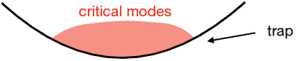
Figure 5: Sketch which highlights the emergence of the critical modes within a trap.

The above considerations apply to general systems of interacting bosonic particles trapped by an external harmonic potential. In particular, we mention bosonic cold atoms in optical lattices [166], which can be effectively described [155] by the BH model [154] defined by the Hamiltonian (26). Experiments with cold atoms [156, 157, 166, 318] are usually performed in the presence of a trapping potential, which can be taken into account by adding a corresponding term in the Hamiltonian:

$$\hat{H}_{\rm tBH}=\hat{H}_{\rm BH}+\sum_{\bm{x}}V_{\bm{x}}\hat{n}_{\bm{x}}\,,\qquad\qquad V_{\bm{x}}=v^{p}|{\bm{x}}|^{p}\,,$$ (80)

where $\hat{H}_{\rm BH}$ is given by Eq. (26), the trap is assumed to be spherical around a center located at ${\bm{x}}=0$, $v$ is a positive constant, and $p$ is a positive exponent. Far from the origin, the potential $V_{\bm{x}}$ diverges, therefore $\langle\hat{n}_{\bm{x}}\rangle$ vanishes and the particles are trapped. In the experiments, one usually has harmonic trapping potentials, that is, $p=2$.

A natural definition of trap size is provided by [166, 327, 324, 347, 318, 224]

$$\ell\equiv{t^{1/p}\over v}\,,\qquad{\rm so}\;\;{\rm that}\quad V_{\bm{x}}=t^{-1}\,\left({|{\bm{x}}|\over\ell}\right)^{p}\,,$$ (81)

where $t$ is the kinetic constant. In the following we set $t=1$. In the limit $p\to\infty$, one recovers the case of a homogeneous system within a $d$-dimensional sphere of radius $\ell$ and OBC, whose scaling behavior is described by the FSS theory discussed previously. The definition (81) of trap size naturally arises when considering the thermodynamic limit for a large number $N$ of particles, which is generally defined by the limit $N,\,\ell\to\infty$ keeping the ratio $N/\ell^{d}$ fixed [347, 166]. This limit turns out to be equivalent to introducing the chemical potential $\mu$, as in Eqs. (80) and (26), i.e., to the limit $\ell\to\infty$ keeping $\mu$ fixed.

4.6.1 Local density approximation of the particle density

The inhomogeneous confining potential gives rise to a particle density that depends on the space, in particular on the distance from the center of the trap, in the case of spherical symmetry. In such cases, theoretical and experimental results have witnessed the coexistence of MI and superfluid regions when varying the total occupancy of the lattice (see, e.g., Refs. [328, 155, 348, 349, 350, 351, 352, 326, 327, 353, 354, 355, 356, 334, 357]).

In the presence of a space-dependent external potential, the so-called local density approximation (LDA) estimates the spatial dependence of the particle density by taking the corresponding value for the homogeneous system at the effective chemical potential

$$\mu_{\rm eff}({\bm{x}})\equiv\mu-V({\bm{x}})\,.$$ (82)

The LDA has been widely used to get quantitative information on the behavior of BH models in a confining potential, and, more generally, of inhomogeneous systems (see, e.g., Refs. [358, 359, 349, 352, 326]).

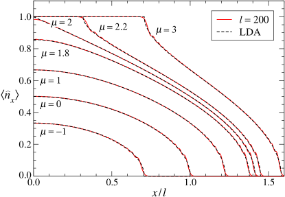
Figure 6: The particle density vs. $x/\ell$ for $p=2$ and several values of the chemical potential $\mu$, as obtained from the LDA, cf. Eq. (83), and numerical calculations on a large chain with $\ell=200$. The differences are hardly visible in the figure. Adapted from Ref. [318].

For example let us consider the $1d$ BH model in the $U\to\infty$ limit. Such model has a nonzero filling above the low-density Mott transition (i.e., for $\mu>-2$). The filling $f$ in the infinite-chain limit $L\to\infty$ is reported in Eq. (76). The corresponding Fermi momentum is $k_{F}=\pi f$. In the following, $f$ will always denote the value for the infinite homogeneous chain. The LDA of the particle density reads

$$\langle\hat{n}_{x}\rangle_{\rm lda}\equiv\rho_{\rm lda}(x/\ell)=\left\{\begin{array}[]{lll}0&\quad{\rm for}&\;\mu_{\rm eff}(x)<-2\,,\\ 1-(1/\pi)\arccos[\mu_{\rm eff}(x)/2]&\quad{\rm for}&\;|\mu_{\rm eff}(x)|\leq 2\,,\\ 1&\quad{\rm for}&\;\mu_{\rm eff}(x)>2\,.\end{array}\right.$$ (83)

This would imply the presence of a plateau at $n=1$ when $\mu_{\rm eff}\geq 2$, for

$$x/\ell\leq(-2+\mu)^{1/p}\,,$$ (84)

and a vanishing particle density when $\mu_{\rm eff}\leq-2$, for

$$x/\ell\geq(2+\mu)^{1/p}\,.$$ (85)

In Fig. 6, the LDA of the particle density is compared with numerical results for $p=2$ and the trap size $\ell=200$ [318]. Note the flat regions related to the $n=0,1$ Mott phases, have been already observed in experimental and numerical works (see, e.g., Refs. [155, 349, 328]). Analogous results are found for other powers of the confining potential. The LDA provides a good approximation of the local particle density, which improves with increasing trap size. The differences of the trap-size dependence from the LDA results are generally suppressed by powers of $\ell$ when increasing $\ell$, and show a nontrivial scaling behavior, also characterized by peculiar modulations [318] (see also below). On the other hand, critical correlation functions between different spatial points, subject to different external forces, require a different framework, which goes beyond LDA.

4.6.2 Trap-size scaling

To investigate the critical behaviors within a trap, for example when the chemical potential is closed to its Mott transition values, a different approach is called for, which allows one to treat the critical fluctuations neglected by the LDA. This issue can be studied within the so-called TSS framework.

We again assume that the zero-temperature quantum critical behavior of the homogeneous system is controlled by one relevant parameter $r\equiv\mu-\mu_{c}$, as described in Sec. 2.3. We suppose that the inhomogeneity arises from an external potential coupled to the particle density, as for the Hamiltonian (80). The presence of the external trapping field significantly affects the critical modes, introducing another length scale, the trap size $\ell$ defined in Eq. (81). Within the TSS framework [173, 306], the scaling of the singular part of the free-energy density around the center of the trap is generally written as 

$$F({\bm{x}};v,T,r)\approx\ell^{-(d+z)\theta}\,{\cal F}(\ell^{-\theta}|{\bm{x}}|,\ell^{\theta z}T,\ell^{\theta y_{r}}r)\,,$$ (86)

where $\theta$ is the trap exponent. TSS implies that at the critical point ($r=0$) the correlation length $\xi$ of the critical modes behaves as

$$\xi\sim\ell^{\theta}$$ (87)

with increasing the trap size $\ell$.

The trap exponent $\theta$ depends on the universality class of the transition, on its space dependence, and on the way it couples to the particles. Its value can be inferred by a RG analysis of the perturbation $P_{V}$ associated with the external trapping potential coupled to the particle density [173, 306]. Since the particle density corresponds to the energy operator $|\phi|^{2}$ of the corresponding field-theoretical description (see Sec. 3.2.2), we write the perturbation $P_{V}$ as

$$P_{V}=\int{\rm d}^{d}x\,{\rm d}t\,V({\bm{x}})\,|\phi({\bm{x}},t)|^{2}=\int{\rm d}^{d}x\,{\rm d}t\,v^{p}|{\bm{x}}|^{p}\,|\phi({\bm{x}},t)|^{2}\,.$$ (88)

The exponent $\theta$ is related to the RG dimension $y_{v}$ of the coupling $v$ of the external field $V=(vr)^{p}$ by $\theta=1/y_{v}$. Then, since the RG dimensions of the terms within space-time integral representing $P_{V}$ must be equal to $d+z$ (that is, the RG dimension of the space and time), we have

$$p\,y_{v}-p+y_{n}=d+z\,,$$ (89)

where $y_{n}=d+z-y_{r}$ is the RG dimension of the density/energy operator $|\phi|^{2}$. We eventually obtain [306]

$$\theta={1\over y_{v}}={p\over p+y_{r}}\,.$$ (90)

Multiplicative logarithms are typically expected at the upper dimension of the given universality class, and also at the BKT transition . Note that in the limit $p\to\infty$, when the trap tends to become equivalent to a system of size $\ell$ with OBC, the exponent $\theta\to 1$, as it should, since in this limit TSS must become equivalent to FSS. Analogous scaling ansatze for other systems in the presence of inhomogeneous external forces have been put forward in Refs. [360, 361, 362, 363, 364, 365].

TSS equations can be derived for the correlation functions of the critical modes. For example, the correlation function of the fundamental complex field $\phi({\bm{x}})$ (the quantum field $\hat{b}$ in the BH model) is expected to behave as

$$G({\bm{x}},{\bm{y}})\equiv\langle\phi({\bm{x}})\,\phi({\bm{y}})\rangle_{c}\approx\ell^{-\theta(d+z-2+\eta)}\,{\cal G}(\ell^{-\theta}{\bm{x}},\,\ell^{-\theta}{\bm{y}},\,\ell^{\theta z}T,\,\ell^{\theta y_{r}}r)\,,$$ (91)

where ${\cal G}$ is a scaling function (the subscript c denotes the connected component ).

Other interesting observables are related to the particle density. At the vacuum-to-superfluid transition, $\mu_{c}=-2d$, the spatial dependence of the particle density is described by the asymptotic TSS [318]

$$\rho_{\bm{x}}\equiv\langle\hat{n}_{\bm{x}}\rangle\approx\ell^{-y_{n}\theta}\,{\cal D}(\ell^{-\theta}{\bm{x}},\,\ell^{\theta z}T)\,,$$ (92)

where $y_{n}$ is the RG dimension of the particle density operator $\hat{n}_{\bm{x}}$, which is given by $y_{n}=d+z-y_{r}$. Its behavior behaviors turn out to be more complicated at the Mott $n\geq 1$ transitions, where modulation phenomena emerge, similar to those appearing in the finite-size behavior within the superfluid phase. The spatial dependence of the particle density turns out to be described by the following scaling behavior:

$$\rho({\bm{x}})\approx\rho_{\rm lda}({\bm{x}}/\ell)+\ell^{-y_{n}\theta}\,{\cal D}(\ell^{-\theta}{\bm{x}},\varphi)\,.$$ (93)

The dominant term in the large trap-size limit is just given by the LDA, which plays the role of an analytical contribution that must be subtracted to observe scaling in the expectation value of the density operators at phase transitions [173, 306]. As noticed in Refs. [318, 338], the scaling function is characterized by a further dependence on a phase (which somehow measures the distance from the closest level crossing), modulating the TSS, arising from periodic level crossings with increasing the system size, analogously to the phenomenon discussed in Sec. 4.5.

The above scaling relations tell us that the LDA is approached in the large trap-size limit, with $O(\ell^{-y_{n}\theta})$ corrections. However, this asymptotic behavior changes close to the boundary of the trap (i.e., when $\rho_{\rm lda}\approx 0$). In this case, the asymptotic approach is controlled by the critical point associated with the vacuum-to-superfluid transition in an effective external linear potential [318, 193].

The trap-size dependence predicted by TSS has been verified at various thermal and quantum transitions: at the Ising transition of lattice gas models [173, 180, 342], at the BKT transitions of spin models [209, 340], at QTs of Ising-like and XY systems (considering in particular their equivalent fermionic systems) [306, 338], at the finite-temperature BEC transition of bosonic particle systems such as those described by the $3d$ BH model [185, 190, 346], at the finite-temperature BKT of $2d$ BH models [196, 193], at the quantum Mott transitions of BH models [306, 318, 343, 344], in fermionic gases [366, 225, 367]. In particle gases with a definite number $N$ of particles, the TSS can be expressed in terms of $N$, being related to the scaling behavior close to the QT separating the vacuum from the superfluid phase, at $\mu_{\textrm{vs}}=-2d$ (see, e.g., Refs. [368, 224, 366, 369, 225, 226]).

5 Equilibrium scaling behavior at first-order quantum transitions

Quantum phase transitions are of the first order when ground-state properties are discontinuous across the transition point. However, singularities develop only in the infinite-volume limit. If the system size $L$ is finite, all the properties are analytic as a function of the external parameter driving the transition. Nevertheless, around the transition point, thermodynamic quantities and large-scale properties develop peculiar scaling behaviors essentially depending on the general features of the transition. Their understanding is essential to correctly interpret experimental or numerical data, which implement relatively small systems.

These issues are also important for FOQTs, essentially for two good reasons. The first one is that FOQTs are phenomenologically relevant, as they occur in a large number of quantum many-body systems, including quantum Hall samples [370], itinerant ferromagnets [371, 372], heavy fermion metals [373, 374, 375], SU($N$) magnets [376, 377], quantum spin systems [150, 55, 378, 379], etc. The second reason is that the low-energy properties at FOQTs are particularly sensitive to the BC, giving rise to a variety of possible scenarios, wider than those at CQTs. Indeed, depending on the type of BC, for example whether they are neutral or they favor one of the phases, the behavior at FOQTs may be characterized by qualitatively different dynamic properties [55, 378, 57, 380, 381, 382], associated with exponential or power-law scaling. Actually, in finite-size systems, this peculiar sensitivity of FOQTs to the BC likely represents the most striking difference with CQTs.

Classical first-order transitions, driven by thermal fluctuations, display FSS behaviors [383, 384, 147, 385, 112, 386, 113, 387, 388, 72], similarly to continuous transitions. On the basis of the general quantum-to-classical mapping of $d$-dimensional quantum systems onto classical anisotropic $(d+1)$-dimensional systems, one expects that the FSS theory of classical first-order transitions can be extended to FOQTs, as put forward in Refs. [55, 378]. However, we recall the comment reported in Sec. 4.1 on the quantum-to-classical mapping, and the intrinsic anisotropy of the resulting classical system. In this respect, FOQTs may lead to extremely anisotropic classical systems, such as for quantum Ising-like systems, characterized by an exponentially larger length scale along the imaginary time, analogously to the classical models considered in Ref. [147]. Therefore, especially at FOQTs, while the quantum-to-classical mapping remains a useful guiding idea, a direct approach using quantum settings is simpler and likely more illuminating than going through the former.

In the following we present the main features of the FSS behavior at FOQTs, describing the different scenarios emerging when various types of BC are considered. We discuss this issue within the paradigmatic quantum Ising models along their FOQT line, separating differently magnetized phases. However most results apply to generic FOQTs as well. We first focus on FSS with neutral BC, where a quasi-level-crossing scenario emerges (Sec. 5.3), and then address BC giving rise to domain walls, leading to a substantially different picture (Sec. 5.4). In Sec. 5.5 we describe the more complex situation arising from BC favoring one of the two magnetized phases. Finally, in Sec. 5.6 we discuss the possibility of observing CQTs along FOQT lines driven by defects only.

Here we only mention, without further addressing it, that peculiar scaling behaviors can be also observed in the presence of inhomogeneous conditions, such as those arising from space-dependent external fields, at both FOQTs [389] and classical first-order transitions [365].

5.1 Finite-size scaling at first-order quantum transitions

We consider a generic finite $d$-dimensional system of size $L$ (as usual, we may assume a cubic-like shape with a volume $L^{d}$), undergoing a FOQT driven by a magnetic field $h$, such as quantum Ising systems defined by the Hamiltonian (6), along the FOQT line for $|g|<g_{c}$. We assume that the BC are such to preserve the parity symmetry at $h=0$. This neutrality of BC is guaranteed by PBC, ABC, and OBC in quantum Ising systems, and also by OFBC in the Ising chains. The preservation of the parity symmetry implies that the minimum of the difference of the lowest states occurs at strictly $h=0$.

At FOQTs, the interplay between the temperature $T$, the field $h$, and the system size $L$ gives rise to an asymptotic FSS of the low-energy properties. To write down the corresponding scaling ansatz, it is necessary to identify the relevant scaling combinations associated with $h$ and $T$. The scaling variable controlling the interplay between $h$ and the size $L$ is naturally provided by the ratio $\Phi$ between the energy variation $\delta E_{h}$ arising from the longitudinal field $h$,

$$\delta E_{h}(L,h)\equiv E(L,h)-E(L,h=0)\,,$$ (94)

and the energy difference (gap) $\Delta(L)$ of the lowest states at $h=0$ [55]. Thus

$$\Phi\equiv\frac{\delta E_{h}(L,h)}{\Delta(L)}\,,\qquad\Delta(L)\equiv\Delta(L,h=0)\,.$$ (95)

At the FOQTs driven by the longitudinal field, for sufficiently small $h$ the difference (94) is given by [55]

$$\delta E_{h}(L,h)=2m_{0}hL^{d}\,,$$ (96)

where $m_{0}$ is the magnetization obtained when approaching the transition point $h\to 0$ after the infinite-volume limit, cf., Eq. (17). The scaling variable controlling the interplay between $T$ and $L$ is naturally defined by the ratio

$$\Xi\equiv{T\over\Delta(L)}\,.$$ (97)

The FSS limit corresponds to $L\to\infty$ and $h\to 0$, keeping $\Phi$ and $\Xi$ fixed. In this limit, the gap $\Delta$ is expected to behave as [55]

$$\Delta(L,h)\approx\Delta(L)\,{\cal E}(\Phi)\,.$$ (98)

By definition ${\cal E}(0)=1$, and ${\cal E}(\Phi)\sim|\Phi|$ for $\Phi\to\pm\infty$, in order to reproduce the expected linear behavior $\Delta(L,h)\sim|h|L^{d}$ for sufficiently large $|h|$. Moreover, the local and global magnetization [such as those defined in Eq. (16)], are expected to scale as

$$m_{\bm{x}}(L,T,h)\approx m_{0}\,{\cal M}_{x}({\bm{x}}/L,\Xi,\Phi)\,,\qquad M(L,T,h)\approx m_{0}\,{\cal M}(\Xi,\Phi)\,.$$ (99)

Because of the definition of $m_{0}$, cf. Eq. (17), we have ${\cal M}(0,\Phi)\to\pm 1$ for $\Phi\to\pm\infty$. Moreover ${\cal M}(T,0)=0$ by parity symmetry. For systems without boundaries, $m_{\bm{x}}(L,T,h)=M(L,T,h)$ by translation invariance, thus ${\cal M}_{x}({\bm{x}}/L,\Xi,\Phi)={\cal M}(\Xi,\Phi)$. The above FSS ansatze represent the simplest scaling behaviors compatible with the discontinuities arising in the thermodynamic limit. The scaling variables $\Phi$ and $\Xi$, associated with $h$ and $T$ respectively, are related to the finite-size energy gap at the transition, whose size behavior depends crucially on the BC considered, disclosing exponential and power-law behaviors, as stated in Sec. 3.1.3. Hence, once they are expressed in terms of the size and of the parameter driving the transition, their $L$-dependence changes according to the chosen BC. As a consequence, the FSS behaviors may be characterized by power laws, as in CQTs, or exponential laws, which are peculiar to FOQTs only.

5.2 Unified scaling picture at first-order and continuous quantum transitions

It is worth noticing that the definitions of $\Phi$ and $\Xi$ in Eqs. (95) and (97) also apply to CQTs, for example at the end point of the FOQT line for quantum Ising models at $g=g_{c}$. Indeed, as discussed in the previous section, the CQT scaling variable associated with the external field $h$ is given by

$$\Phi=L^{y_{h}}h\,,$$ (100)

which can be obtained using the more general definition (95). Indeed, at CQTs the energy variation $\delta E$ arising from the perturbation

$$\hat{H}_{h}=-h\sum_{\bm{x}}\hat{P}_{\bm{x}}\,,\qquad\hat{P}_{\bm{x}}=\hat{\sigma}^{(1)}_{\bm{x}}\,,$$ (101)

behaves as

$$\delta E_{h}(L,h)\sim h\,L^{d-y_{p}}\,,$$ (102)

where $y_{p}$ is the RG critical dimension of the local operators $\hat{P}_{\bm{x}}$ at the fixed point describing the quantum critical behavior. Moreover, at $g=g_{c}$, we have $\Delta(L,h=0)\sim L^{-z}$ where $z$ is the universal dynamic exponent. Then, using the scaling relation among the critical exponents [86, 1]

$$y_{h}+y_{p}=d+z\,,$$ (103)

where $y_{h}$ is the RG dimension of the perturbation $h$, we end up with the expression for $\Phi$ reported in Eq. (100). Analogously, using Eq. (97) and $\Delta\sim L^{-z}$, we recover the CQT scaling variable $\Xi=L^{z}\,T$. Therefore, the definitions (95) and (97) for the scaling variables provide a unified FSS framework for CQTs and FOQTs. The differences are encoded within the size dependence of $\Phi$ and $\Xi$.

5.3 Neutral boundary conditions giving rise to a quasi-level-crossing scenario

We now consider a class of BC that are neutral with respect to the different phases separated by the FOQTs. For quantum Ising models, where FOQTs are driven by the longitudinal field $h$, such BC are provided by PBC or OBC. In these cases the expected scenario is that of a quasi-level-crossing of the two lowest states, with exponentially suppressed energy differences $\Delta\sim\exp(-cL^{d})$ of the lowest states, such as Eqs. (18), (19a) and (19b), while the energy differences $\Delta_{n}$ associated with higher excited states remain finite (or more generally $\Delta_{n}/\Delta\to\infty$ exponentially, apart from power laws) in the infinite-volume limit. The general FSS theory outlined in Sec. 5.1 implies scaling variables $\Phi$ and $\Xi$ with an exponential dependence on the lattice size, through the exponential suppression of the gap in the large-$L$ limit. The corresponding FSS functions, such as those introduced in Eqs. (98) and (99), can be computed by exploiting a phenomenological two-level theory, as explained below.

For sufficiently large $L$, the low-energy properties in the crossover region $|h|\ll 1$ can be obtained by restricting the theory to the two lowest-energy states $|0\rangle$ and $|1\rangle$, or equivalently to the globally magnetized states $|+\rangle$ and $|-\rangle$, exploiting a two-level truncation of the spectrum [55, 390]. The effective evolution is ruled by the Schrödinger equation

$${{\rm d\,|\Psi_{2}(t)\rangle}\over{\rm d}t}=-i\,\hat{H}_{2}(h)\,|\Psi_{2}(t)\rangle\,,$$ (104)

where $|\Psi_{2}(t)\rangle$ is a two-component wave function, whose components correspond to the states $|+\rangle$ and $|-\rangle$, and

$$\hat{H}_{2}(h)=\varepsilon\,\hat{\sigma}^{(3)}+\zeta\,\hat{\sigma}^{(1)}\,.$$ (105)

Here $\varepsilon$ is related to the perturbation induced by the magnetic field $h$, while $\zeta$ is related to the small gap $\Delta(L)$ at $h=0$ [55],

$$\varepsilon=m_{0}hL^{d}\,,\qquad\zeta=\langle-|\hat{H}_{\rm Is}|+\rangle=\tfrac{1}{2}\,\Delta(L,h=0)\,,$$ (106)

so that one may easily see the correspondence between the scaling variable $\Phi$ of the Ising system and the ratio $\varepsilon/\zeta$,

$$\varepsilon/\zeta\to\Phi\,.$$ (107)

By diagonalizing the restricted Hamiltonian $\hat{H}_{2}$, we obtain the energy difference corresponding to $\Delta(L,h)$. Moreover, by taking the matrix element of the operator $\hat{\sigma}^{(3)}$, we get the quantity corresponding to the magnetization of the quantum Ising model. Then, by matching with the scaling equations (98) and (99), one easily obtains [55]

$${\cal E}(\Phi)=\sqrt{1+\Phi^{2}}\,,\qquad\qquad{\cal M}_{\bm{x}}({\bm{x}}/L,0,\Phi)={\cal M}(0,\Phi)={\Phi\over\sqrt{1+\Phi^{2}}}\,.$$ (108)

Note that in the case of OBC, the above behavior for the local magnetization should hold for lattice sites ${\bm{x}}$ sufficiently far from the boundaries. For sufficiently small temperatures (i.e., $T\sim\Delta$, thus finite $\Xi$), the extension to finite-temperature results can be obtained by averaging over the two levels with the Gibbs weight, i.e.,

$$M=Z_{2}^{-1}\,{\rm Tr}\big{[}\hat{\sigma}^{(3)}e^{-\hat{H}_{2}/T}\big{]}\,,\qquad Z_{2}={\rm Tr}\big{[}e^{-\hat{H}_{2}/T}\big{]}\,.$$ (109)

The results of the above phenomenological two-level theory are expected to be exact for quantum Ising models with neutral BC such as PBC and OBC, i.e., they are expected to be exactly approached in the large-$L$ limit. This has been confirmed by means of computations within quantum Ising chains with OBC [55]. The above approach can be easily extended to the case of a larger finite (quasi) degeneracy of the lowest states, such as quantum Potts models [378].

Low-dimensional systems at FOQTs react rigidly to external local fields $h_{\bm{x}}$ [55]. This property was checked for Ising chains in which the external magnetic field is nonvanishing only at one lattice site $x$, for example at the center of the chain. The general arguments should apply to this case as well, with $\varepsilon\sim 2m_{0}h_{x}$ instead of $\varepsilon=2m_{0}hL$. Therefore, we expect a FSS behavior analogous to that valid for the homogeneous parallel field, the corresponding scaling variable being $\Phi_{x}=2m_{0}h_{x}/\Delta(L)$. Numerical results for the Ising chain are in full agreement with these scaling predictions [55].

We finally mention that, in principle, the above scaling ansatze can be derived by exploiting the general quantum-to-classical mapping, which allows one to map the quantum system onto a classical one defined in an anisotropic box of volume $V=L^{d}\,L_{T}$, with $L_{T}\sim 1/T$ and $L_{T}\gg L$. Then the above results can be also obtained from those reported in Ref. [147] for $(d+1)$-dimensional Ising-like systems at a classical first-order transition with PBC along a transverse dimension. 

5.4 Boundary conditions giving rise to domain walls

The general FSS behaviors reported in Sec. 5.1 also hold in systems at FOQTs with an infinite degeneracy of the ground state at the transition, such as those with BC giving rise to domain walls. For example, let us consider the Ising chain with ABC or OFBC. In these two cases, the lowest-energy states are associated with domain walls (kinks), i.e., nearest-neighbor pairs of antiparallel spins, which can be considered as one-particle states with $O(L^{-1})$ momenta. Hence, there is an infinite number of excitations with a gap of order $L^{-2}$, cf. Eq. (21).

Applying the general FSS theory of Sec. 5.1 to this case, we obtain scaling variables $\Phi$ and $\Xi$ with a power-law dependence on $L$. Indeed, we have

$$\Phi\sim L^{3}\,h\,,\qquad\Xi\sim L^{2}\,T\,.$$ (110)

The scaling ansatze (98) and (99) also hold in this case [55, 57]. Indeed, as shown in Fig. 7, the ratios $\Delta(L,h)/\Delta(L)$ and $M(L,h)/m_{0}$ approach universal (independent of $g$) scaling curves, when plotted versus $\Phi$. However, in this case, scaling functions cannot be obtained by performing a two-level truncation, because the low-energy spectrum at the transition point presents a tower of excited states with $\Delta_{n}=E_{n}-E_{0}=O(L^{-2})$, at variance with the OBC and PBC case, where only two levels matter, close to the transition point.

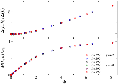
Figure 7: FSS of the energy difference of the lowest states and magnetization of the quantum Ising chain with OFBC, at $g=1/2$ and $g=3/4$. The two panels show data for the ratios $\Delta(L,h)/\Delta(L)$ (top) and $M(L,h)/m_{0}$ (bottom) versus $\Phi=2m_{0}hL/\Delta(L)$. The data approach nontrivial scaling curves with increasing $L$, which are independent of $g$, supporting the FSS Eqs. (98) and (99). Adapted from Ref. [55].

These results reveal that the FSS at FOQTs may significantly depend on the BC, being strictly connected with the large-volume low-energy structure of the eigenstates. This implies the possibility of observing FSS with either exponential or power-law size dependence, due to the fact that $\Phi$ may show either exponential or power-law dependences with $L$, for different BC. For instance, for the Ising chain one has: (i) $\Phi\sim hLe^{\alpha L}$ for OBC; (ii) $\Phi\sim hL^{3/2}e^{\alpha L}$ for PBC ($\alpha$ is a nonuniversal positive constant); (iii) $\Phi\sim hL^{3}$ for ABC or OFBC. This sensitivity to the BC is likely the main feature distinguishing FOQT and CQT behaviors in finite-size systems.

5.5 Boundary conditions favoring one of the two phases

Another interesting case is provided by quantum Ising chains with equal and fixed BC (i.e., EFBC), favoring one of the two magnetized phases. They can be selected by restricting the Hilbert space to states $|s\rangle$ at the boundaries $x=0$ and $x=L+1$ of an open-ended chain, such that $\hat{\sigma}^{(1)}_{0}|s\rangle=-|s\rangle$ and $\hat{\sigma}^{(1)}_{L+1}|s\rangle=-|s\rangle$. As numerically shown in Ref. [380], the interplay between the size $L$ and the bulk longitudinal field $h$ is more complex than that observed with neutral BC. In the case of EFBC, for small values of $h$, observables depend smoothly on $h$, up to $h_{tr}(L)\approx c/L$ ($c$ is a $g$-dependent constant), where a sharp transition to the oppositely magnetized phase occurs, see Fig. 8. The field $h_{tr}(L)$ can be identified as the value of $h$ where the energy difference $\Delta(L,h)$ of the lowest states is minimum. Such a minimum $\Delta_{m}(L)$ turns out to decrease exponentially with increasing $L$, i.e., $\Delta_{m}(L)\sim e^{-bL}$.

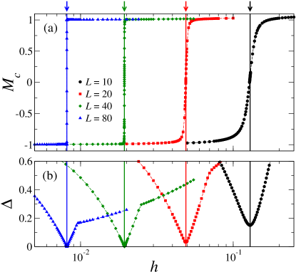
Figure 8: Central magnetization $M_{c}\equiv m_{L/2}/m_{0}$ (normalized so that it ranges from -1 to 1) [panel (a)] and energy gap $\Delta$ [panel (b)] in the quantum Ising chain with EFBC, as a function of the longitudinal field $h$, for fixed transverse field $g=0.8$. The various data sets correspond to different system sizes, as indicated in the legend. The continuous vertical lines and arrows denote the magnetic fields $h_{tr}(L)$ corresponding to the minimum of the energy gap, as displayed in panel (b). From Ref. [380].

In proximity of $h_{tr}(L)$, a universal FSS behavior emerges from the competition of the two lowest-energy states, separated by a gap which vanishes exponentially with $L$. For $h$ close to $h_{tr}(L)$, it is still possible to define a FSS behavior in terms of the scaling variable

$$\Phi_{tr}\equiv{2m_{0}L\,[h-h_{tr}(L)]\over\Delta_{m}(L)}\,,$$ (111)

where $\Delta_{m}(L)$ is the minimum of the energy difference between the two lowest states, defining the location of the pseudotransition point $h_{tr}(L)$ at finite $L$. The scaling variable $\Phi_{tr}$ is the analogue of $\Phi$ defined in Eq. (95), with the essential difference that the finite-size pseudotransition now occurs at $h=h_{tr}(L)$, and not at $h=0$. Therefore, the relevant magnetic energy scale is the difference between the magnetic energy at $h$ and that at $h_{tr}(L)$, while the relevant gap is the one at $h_{tr}(L)$. For $h\approx h_{tr}(L)$, observables are expected to develop a FSS behavior, such as

$$\Delta(L,h)\approx\Delta_{m}(L)\,{\cal E}_{f}(\Phi_{tr})\,,\qquad M_{c}(L,h)\approx{\cal M}_{cf}(\Phi_{tr})\,,$$ (112)

where $M_{c}(L,h)\equiv m_{L/2}(L,h)/m_{0}$ is the normalized magnetization at the center of the chain. These predictions are nicely supported by the data, as visible in Fig. 9. Further details can be found in Ref. [380].

The infinite-volume critical point $h=0$ lies outside the region in which FSS holds. Note that a crucial issue in the definition of the scaling variable $\Phi_{tr}$ is that the values of $h_{tr}(L)$ and $\Delta_{m}(L)$ must be those associated with the minimum of the gap for the given size $L$, i.e., they cannot be replaced with their asymptotic behaviors.

Analogous behaviors are expected in other FOQTs, for example in higher dimensions, when BC favor one of the two phases.

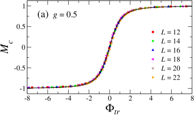
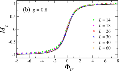
Figure 9: The central magnetization $M_{c}$, defined in Fig. 8, versus the scaling variable $\Phi_{tr}$, for several system sizes (see legend). Panel (a) is for $g=0.5$, while panel (b) is for $g=0.8$. Even though the scenario is more complex than that for OBC (see Sec. 5.3), a two-level model turns out to reproduce the scaling functions (continuous black curve). Adapted from Ref. [380].

5.6 Quantum transitions driven by defects

The driving parameters of QTs are usually bulk quantities, such as the chemical potential in particle systems, or external magnetic fields in spin systems. In the presence of FOQTs, the bulk behavior is particularly sensitive to the BC or to localized defects. This property makes it possible to induce a related CQT by changing only the parameters associated with localized defects or parameters controlling the boundaries [56, 57]. Examples of this type of QTs can be observed in quantum Ising rings with a localized defect.

We consider Ising rings of size $L=2\ell+1$ with a transverse magnetic field and one bond defect:

$$\hat{H}_{r}=-J\sum_{x=-\ell}^{\ell-1}\hat{\sigma}^{(1)}_{x}\hat{\sigma}^{(1)}_{x+1}-g\sum_{x=-\ell}^{\ell}\hat{\sigma}^{(3)}_{x}-\zeta\;\hat{\sigma}_{-\ell}^{(1)}\hat{\sigma}_{\ell}^{(1)}\,.$$ (113)

We again set $J=1$ and assume $g\geq 0$. Varying $\zeta$, it is possible to recover models with PBC, OBC, and ABC, for $\zeta=1$, 0, and $-1$, respectively. The bond defect generally breaks translation invariance, unless $\zeta=\pm 1$. In the presence of an additional parallel field $h$ coupled to $\hat{\sigma}^{(1)}_{x}$, FOQTs occur for any $g<1$.

For $g<1$, we distinguish two phases: a magnet phase ($\zeta>-1$) and a kink phase ($\zeta\leq-1$). The lowest states of the magnet phase are superpositions of states $|\pm\rangle$ with opposite nonzero magnetization $\langle\pm|\hat{\sigma}_{x}^{(1)}|\pm\rangle=\pm m_{0}$ (neglecting local effects at the defect), where${}^{~{}\ref{foot1}}$ $m_{0}=(1-g^{2})^{1/8}$. For a finite chain, tunneling effects between the states $|+\rangle$ and $|-\rangle$ lift the degeneracy, giving rise to an exponentially small gap $\Delta(L,\zeta>-1)$ [391, 392] . An analytic calculation for $\zeta\to-1^{+}$ gives [56, 57]

$$\Delta(L,\zeta\to-1^{+})\approx{8g\over 1-g}w^{2}e^{-wL},\qquad w={1-g\over g}\;(1+\zeta)\,.$$ (114)

The large-$L$ two-point function is trivial,

$$G(x_{1},x_{2})\equiv\big{\langle}\hat{\sigma}_{x_{1}}^{(1)}\,\hat{\sigma}_{x_{2}}^{(1)}\big{\rangle}\to m_{0}^{2}$$ (115)

for $x_{1}\neq x_{2}$, keeping $X_{i}\equiv x_{i}/\ell$ fixed (but $X_{i}\neq\pm 1$).

The low-energy behavior drastically changes for $\zeta\leq-1$, in which the low-energy states are one-kink states (made of a nearest-neighbor pair of antiparallel spins), behaving as one-particle states with $O(L^{-1})$ momenta. In particular, for $\zeta=-1$, corresponding to a system with ABC, the gap decreases as $\Delta(L,-1)\sim L^{-2}$, cf. Eq. (21). The first two excited states are degenerate, thus $\Delta_{2}(L,-1)=\Delta_{1}(L,-1)\equiv\Delta(L,-1)$. For $\zeta<-1$, the ground state and the first excited state are superpositions with definite parity of the lowest kink $|\!\downarrow\uparrow\rangle$ and antikink $|\!\uparrow\downarrow\rangle$ states. The gap in this regime decreases as $L^{-3}$ [148, 392, 56], more precisely

$$\Delta(L,\zeta<-1)={8\zeta g^{2}\over(1-\zeta^{2})(1-g)^{2}}\,{\pi^{2}\over L^{3}}+O(L^{-4})\,.$$ (116)

On the other hand, $\Delta_{n}\equiv E_{n}-E_{0}$ for $n\geq 2$ behaves as $L^{-2}$,

$$\Delta_{2}={3g\over(1-g)}\,{\pi^{2}\over L^{2}}+{6(1-\zeta)g^{2}\over(1+\zeta)(1-g)^{2}}\,{\pi^{2}\over L^{3}}+O(L^{-4})\,.$$ (117)

Corresponding changes are found in the asymptotic behavior of the two-point function [56, 57]

$${G(x_{1},x_{2})\over m_{0}^{2}}=\left\{\begin{array}[]{ll}1-|x_{1}-x_{2}|/\ell&\;{\rm for}\;\;\zeta=-1\,,\vspace*{1mm}\\ 1-|x_{1}-x_{2}|/\ell-|\sin(\pi x_{1}/\ell)-\sin(\pi x_{2}/\ell)|/\pi&\;{\rm for}\;\;\zeta<-1\,.\end{array}\right.$$ (118)

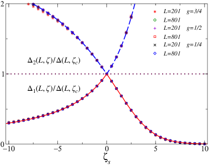
Figure 10: The scaling functions ${\cal D}_{n}(\zeta_{s})$ of Eq. (119) (dashed lines) and numerical data (symbols) for the ratio $\Delta_{n}(L,\zeta)/\Delta(L,\zeta_{c})$ as functions of the scaling variable $\zeta_{s}$, for $n=1$ (bottom) and $n=2$ (top), separated by the dotted line. Numerical data clearly approach the $g$-independent scaling curves ${\cal D}_{n}(\zeta_{s})$ (differences are hardly visible). Adapted from Ref. [56].

The above behaviors show that the defect parameter $\zeta$ drives a QT at $\zeta_{c}=-1$, separating the magnet and kink phases. Moreover the system develops a universal $g$-independent scaling behavior [56], such as

$$\Delta_{n}(L,\zeta)\equiv E_{n}(\zeta)-E_{0}(\zeta)\approx\Delta(L,\zeta_{c})\>{\cal D}_{n}(\zeta_{s})\,,\qquad\zeta_{s}\equiv{1-g\over g}(\zeta-\zeta_{c})\,L\,,$$ (119)

for $L\to\infty$, keeping the scaling variable $\zeta_{s}$ fixed. The scaling functions ${\cal D}_{1}$ and ${\cal D}_{2}$, which have been computed analytically, are shown in Fig. 10, where they are also compared with some numerical results that support the scaling ansatz (119). The cusp-like behavior at $\zeta_{s}=0$ is the consequence of the crossing of the first two excited states at $\zeta=-1$. The asymptotic large-$L$ behavior is generally approached with $O(L^{-1})$ corrections. Other observables satisfy analogous scaling relations, such as the two-point function, and corresponding susceptibility and correlation lengths. An analogous magnet-to-kink QT can be observed in the Ising chain by appropriately tuning a magnetic field coupled to $\hat{\sigma}^{(1)}$, localized at the boundaries. 

The above results reflect a QT with critical exponents given by the RG dimension $y_{\zeta}=1$ of the relevant defect parameter, and dynamic exponent $z=2$ due to the $L^{-2}$ behavior of the gap at $\zeta_{c}$, see Eq. (21). This defect-driven CQT characterizes the FOQT line of the Ising chain. It is worth noting that, at the critical value $g=1$, corresponding to the order-disorder continuous transition, the bulk behavior is independent of the BC or of the presence of defects, hence the magnet-to-kink transition only occurs for $g$ strictly less than 1. For instance, the gap at $g=1$ behaves as $\Delta\sim L^{-1}$ for any $\zeta$ 

In conclusion, peculiar QTs can be induced by tuning the BC or by changing lower-dimensional defect parameters, when the system is at a FOQT. These scaling behaviors can be straightforwardly extended to allow for a nonzero temperature $T$, by considering a further dependence on the scaling variable $\Xi=L^{z}\,T$. Even though we have discussed the issue in $1d$, the same type of behavior is expected in quantum $d$-dimensional Ising models defined in $L^{d-1}\times\bar{L}$ boxes with $L\gg\bar{L}$, in the presence of a $(d-1)$-dimensional surface of defects or of opposite magnetic fields on the $L^{d-1}$ boundaries.

6 Quantum information and many-body systems

In this section we provide an overview of some concepts founded on the recently developing quantum information science [394, 395, 396], which have been proven useful to spotlight the presence of singularities at QTs in many-body systems. Among them, we mention the fidelity and its susceptibility, the quantum Fisher information, as well as the entanglement and other quantifiers of nonclassical correlations. As we shall see in the following, the net advantage of these approaches is that they do not rely on the identification of an order parameter with the corresponding symmetry-breaking pattern, and thus may be helpful also to detect topological transitions. Other specific reviews on these topics can be found in Refs. [397, 398, 399].

6.1 Fidelity and Loschmidt amplitude

The strategy lying at the basis of the concept of fidelity in a quantum many-body system is based on the comparison between two given states of such a system, and quantifies the absolute value of the overlap between them [400]. To fix the ideas, consider for example the ground state $|\Psi_{0}(g)\rangle$ of a given Hamiltonian operator $\hat{H}(g)$, which depends on a control parameter $g$ (it can be the intensity of an external magnetic field, the strength of interactions, or some other parameter). We define the fidelity

$$A(g_{1},g_{2})\equiv\big{|}\langle\Psi_{0}(g_{1})|\Psi_{0}(g_{2})\rangle\big{|}$$ (120)

as a measure of the distance between two ground states at different values of $g$, say $g_{1}$ and $g_{2}$ . Clearly $0\leq A\leq 1$, where $A=1$ if $|\Psi_{0}(g_{1})\rangle$ coincides with $|\Psi_{0}(g_{2})\rangle$ up to a global phase, while $A=0$ if such two states are orthogonal. Now suppose to compare two infinitesimally close parameters, i.e., $g_{1}=g_{2}+\varepsilon$. It is rather intuitive that in proximity of a QT, when the system observables may undergo singular behaviors, even the slightest move in $g$ may result in a considerable deviation of $A$ from the unit value, showing that the two ground states increase their degree of orthogonality [401].

The fidelity can be a convenient tool also to address the sensitivity of the quantum motion under Hamiltonian perturbations. In fact this is the original context where it was first introduced [402], in the framework of quantum chaos, and recently extended to the many-body realm. The setting can be put under the following general grounds: From a given pure state $|\Psi_{\rm in}\rangle$ (not necessarily the ground state), one can construct two state vectors $|\Psi(t)\rangle$ and $|\Psi_{\varepsilon}(t)\rangle$ according to the unitary evolutions ruled by $\hat{H}(g)$ and $\hat{H}(g+\varepsilon)$, respectively. The fidelity is the absolute value of the overlap between them, namely

$$A_{\varepsilon}(t)=\big{|}\langle\Psi(t)|\Psi_{\varepsilon}(t)\rangle\big{|}\,,$$ (121)

with

$$|\Psi(t)\rangle=e^{-i\hat{H}(g)t}|\Psi_{\rm in}\rangle\qquad\mbox{and}\qquad|\Psi_{\varepsilon}(t)\rangle=e^{-i\hat{H}(g+\varepsilon)t}|\Psi_{\rm in}\rangle\,.$$ (122)

The above expression (121), without taking the absolute value, is called the Loschmidt amplitude $\widetilde{A}_{\varepsilon}(t)=\langle\Psi(t)|\Psi_{\varepsilon}(t)\rangle=\langle\Psi_{\rm in}(t)|e^{i\hat{H}(g)t}\,e^{-i\hat{H}(g+\varepsilon)t}|\Psi_{\rm in}\rangle$, since it can be equivalently seen as the overlap between a given state and the one obtained by first evolving forward-in-time with t¡he unitary operator $e^{-i\hat{H}(g+\varepsilon)\,t}$, followed by a backward-in-time perturbed evolution under $e^{-i\hat{H}(g)\,t}$.

We finally mention that the definition of the fidelity in Eq. (120) can be generalized also to the cases in which one or both (pure) states are substituted by mixed states. Namely, the fidelity $A\in[0,1]$ between a given pure state $|\psi\rangle$ and a mixture $\rho$ is given by

$$A(|\psi\rangle,\rho)\equiv\sqrt{\langle\psi|\rho|\psi\rangle}\,,$$ (123)

while the fidelity between two mixtures $\rho$ and $\sigma$ is defined by [403]

$$A(\rho,\sigma)\equiv{\rm Tr}\left[\sqrt{\sigma^{1/2}\rho\,\sigma^{1/2}}\,\right]\,,$$ (124)

where ${\rm Tr}[\,\cdot\,]$ indicates the trace operation.

6.2 State discrimination and the quantum Fisher information

The concept of fidelity is intimately related to the quantum estimation theory, which can be put on formal grounds through the quantum Cramér-Rao bound [404, 405]. Indeed the latter sets the limits on the precision that can be attained in the estimation of an unknown parameter $\lambda$ from repeated independent measurements of the quantum system. Namely, suppose to have a family of quantum states $\{\rho_{\lambda}\}$ that depend on $\lambda$ . Then, the variance of the estimated quantity $(\Delta\lambda)^{2}$ should be limited by

$$(\Delta\lambda)^{2}\geq\frac{1}{MA_{Q}(\rho_{\lambda})}\,,$$ (125)

where $M$ is the number of times the measurement is repeated and $A_{Q}$ is the so-called quantum Fisher information of the state $\rho_{\lambda}$. The quantum Fisher information can be expressed as

$$A_{Q}(\rho_{\lambda})=8\lim_{\delta\lambda\to 0}\frac{1-A(\rho_{\lambda},\rho_{\lambda+\delta\lambda})}{\delta\lambda^{2}}\,,$$ (126)

where $A(\rho_{\lambda},\rho_{\lambda+\delta\lambda})$ is the fidelity between two mixed states, defined in Eq. (124). In fact, the right-hand side of Eq. (126) quantifies the susceptibility of the quantum state to infinitesimal variations of the parameter $\lambda$ and thus defines the fidelity susceptibility (see also Sec. 7.1.1). 

The quantum Fisher information plays a crucial role in quantum metrology, since it determines the reachable accuracy of the estimated quantity [406]: through the above quantum Cramér-Rao bound (125), it may be possible to identify which resources (e.g., entanglement or squeezing) are useful to improve the measurement accuracy, as well as the proper procedures to adopt to fully exploit them [407].

6.3 Entanglement

The concept of entanglement is one of the cornerstones of quantum information theory and arises from the necessity to distinguish the quantum correlations, that can occur in many-body quantum states, from the classical ones [408, 409]. Such distinction can be made rigorous by first defining the amount of classical correlations, a concept that relies on the possibility to perform local operations supplemented by classical communication (LOCC) between partitions that compose the whole system. Any other correlations, that cannot be simulated by the above means, are associated with quantum effects and labelled as quantum correlations. As described below, it is possible to provide different types of quantifiers for the entanglement, which treat it as an operational resource to perform tasks that are impossible, if the quantum state is separable.

To be more precise, let us first consider a bipartite system (i.e., a system made of two parts $\tt{A}$ and $\tt{B}$, typically called Alice and Bob, to use the quantum information jargon) in a pure state $|\psi\rangle_{\tt{AB}}$. Such a state is called separable if and only if it can be written as

$$|\psi\rangle_{\tt{AB}}=|\alpha\rangle_{\tt A}\otimes|\beta\rangle_{\tt B}\,,$$ (127)

where $\otimes$ denotes the tensor product, while the (pure) states $|\alpha\rangle_{\tt A}$ and $|\beta\rangle_{\tt B}$ respectively describe the components of the two parts. Any state $|\psi\rangle_{\tt{AB}}$ that cannot be written as in Eq. (127) (that is, a non-separable state) is named entangled. The above definition of separability can be easily generalized to the case of a bipartite mixed state:

$$\rho_{\tt{AB}}=\sum_{k}p_{k}\,\rho_{\tt A}^{(k)}\otimes\rho_{\tt B}^{(k)}\,,\qquad\mbox{with }\;\;p_{k}\geq 0\,,\;\;\sum_{k}p_{k}=1\,,$$ (128)

$\rho_{\tt A}^{(k)}$ and $\rho_{\tt B}^{(k)}$ being density matrices for the corresponding two parts, and also to the more general case of a $n$-partite system, made of parts $\tt{A,B,C,}\ldots$, according to the following:

$$\rho_{\tt{ABC\ldots}}=\sum_{k}p_{k}\,\rho_{\tt A}^{(k)}\otimes\rho_{\tt B}^{(k)}\otimes\rho_{\tt C}^{(k)}\otimes\ldots\,.$$ (129)

Analogously as for pure states, mixed states that are not separable are named entangled.

Finding quantifiers of nonclassical correlations is, in general, a difficult task, however any good entanglement measure $\mathcal{E}$ shall fulfill a number of reasonable requirements. For the sake of simplicity, here we restrict the discussion to the case of the bipartite entanglement $\mathcal{E}(\rho_{\tt{AB}})$, where the situation is somewhat simpler to describe. The more involved cases of $n$-partite scenarios will be briefly addressed below in Sec. 6.5.

The quantity $\mathcal{E}$ can be defined according to the following:

1. It shall be a map from arbitrary density operators $\rho_{\tt{AB}}$ of a bipartite quantum system to positive real numbers. The measure should be normalized in such a way that there exist maximally entangled states (states, or a class of states, that are more entangled than all the others). These can be shown to be equivalent, up to unitary operations, to the generalized Einstein-Podolsky-Rosen (EPR) [408] pair

   $$|\phi^{+}_{d}\rangle_{\tt{AB}}=\frac{1}{\sqrt{d}}\,\Big{(}|0\rangle_{\tt A}\otimes|0\rangle_{\tt B}+|1\rangle_{\tt A}|\otimes|1\rangle_{\tt B}+\;\ldots\;+|d-1\rangle_{\tt A}|\otimes|d-1\rangle_{\tt B}\Big{)}\,,$$ (130)

   where $d$ is the dimension of each of the two subsystems.

2. It should not increase under LOCC.

3. It should vanish for any separable state.

Any function $\mathcal{E}(\rho_{\tt{AB}})$ satisfying these three conditions is called an entanglement monotone. Examples of such monotones are the entanglement cost and the distillable entanglement. The first one is defined as the rate of maximally entangled states needed to create $\rho_{\tt{AB}}$ using LOCC. The second one quantifies the complementary optimal rate of maximally entangled states that can be distilled from $\rho_{\tt{AB}}$ using LOCC. We also mention the entanglement of formation, being constructed as the minimal possible average entanglement over all the pure-state decompositions of $\rho_{\tt{AB}}$.

There are other requirements one should expect to enforce, even if it could be complicated to construct a measure satisfying all of them. In particular $\mathcal{E}$ should satisfy:

1. Continuity, in the sense that, for decreasing distance between two density matrices, the difference between their entanglement should tend to zero.

2. Convexity: $\mathcal{E}(\sum_{i}p_{i}\rho_{i})\leq\sum_{i}p_{i}\,\mathcal{E}(\rho_{i})$, where $p_{i}>0$, $\sum_{i}p_{i}=1$.

3. Additivity: $\mathcal{E}(\rho^{\otimes n})=n\,\mathcal{E}(\rho)$.

4. Subadditivity: $\mathcal{E}(\rho\otimes\sigma)\leq\mathcal{E}(\rho)+\mathcal{E}(\sigma)$.

6.3.1 Bipartite entropies

For bipartite pure states $\rho_{\tt{AB}}=|\psi\rangle_{\tt{AB}}\langle\psi|$, it is possible to define a unique measure of entanglement $\mathcal{E}(|\psi\rangle_{\tt{AB}})$ satisfying all the above conditions and coinciding with the above mentioned entanglement monotones. This is the von Neumann entropy $S$ of the reduced density matrix of one of the two parts, say Alice: $\rho_{\tt{A}}={\rm Tr}_{\tt B}[|\psi\rangle_{\tt{AB}}\langle\psi|]$ (where ${\rm Tr}_{\tt{B}}[\,\cdot\,]$ denotes the partial trace over Bob), also referred to as the entropy of entanglement,

$$\mathcal{E}(|\psi\rangle_{\tt{AB}})=S(\rho_{\tt A})\equiv-{\rm Tr}\big{[}\rho_{\tt A}\log\rho_{\tt A}\big{]}\,,$$ (131)

which is thus a nonlinear function of the eigenvalues of $\rho_{\tt A}$ .

Relaxing some of the requirements above, as for example the subadditivity, one can define other bipartite entanglement measures which are grouped under the name of Rényi entropies $S_{n}$, defined as

$$S_{n}(|\psi\rangle_{\tt{AB}})\equiv\frac{1}{1-n}\log{\rm Tr}\big{[}\rho_{\tt A}^{n}\big{]}\,,$$ (132)

for any real number $n\geq 0$ and $n\neq 1$. For $n\to 1$ one recovers the von Neumann entropy $S$ in Eq. (131). These quantities, although not fulfilling all the expected properties of entanglement measures, are often employed in the study of quantum many-body systems, since they are typically easier to compute than the von Neumann entropy.

6.3.2 Concurrence

The situation is definitely more complex for bipartite mixed states $\rho_{\tt{AB}}\neq|\psi\rangle_{\tt{AB}}\langle\psi|$, where the above mentioned entanglement monotones do not coincide and, in general, finding operative ways to define and calculate good entanglement measures is cumbersome. One of the scarce cases where this is possible are mixed states of two spin-$1/2$ particles (also named qubits), where there exists a measure called the concurrence [410]. The concurrence $C$ is equivalent to the entanglement of formation and is defined as

$$C(\rho_{\tt{AB}})\equiv\max\big{\{}0,\lambda_{1}-\lambda_{2}-\lambda_{3}-\lambda_{4}\big{\}}\,,$$ (133)

where $\lambda_{i}$ are the square roots of the eigenvalues, in descending order, of the Hermitian matrix

$$R=\sqrt{\rho}\,\tilde{\rho}\,\sqrt{\rho}\qquad\mbox{with }\;\tilde{\rho}=\big{(}\hat{\sigma}^{(2)}\otimes\hat{\sigma}^{(2)}\big{)}\,\rho^{\star}\,\big{(}\hat{\sigma}^{(2)}\otimes\hat{\sigma}^{(2)}\big{)}\,,$$ (134)

where the complex conjugation is taken in the basis of $\hat{\sigma}^{(3)}$.

6.3.3 Other entanglement indicators

There are other bipartite entanglement measures that can be useful in different situations. Among them, we mention the negativity $\mathcal{N}$, which is based on the partial transpose of the density matrix $\rho_{\tt{AB}}$ with respect to one of the subsystems, namely $\rho^{T_{\tt{A}}}_{\tt{AB}}=(\hat{T}_{\tt{A}}\otimes\hat{I}_{\tt{B}})\rho_{\tt{AB}}$, where $\hat{T}_{\tt{A}}$ is the transpose operator acting on Alice, and $\hat{I}_{\tt{B}}$ the identity operator acting on Bob. The negativity is defined as [411]

$$\mathcal{N}\equiv\sum_{\tilde{\lambda}_{i}<0}|\tilde{\lambda}_{i}|\,,$$ (135)

with $\tilde{\lambda}_{i}$ indicating the negative eigenvalues of $\rho^{T_{\tt{A}}}_{\tt{AB}}$. Unfortunately, the negativity assigns non-vanishing entanglement only to a subset of all the entangled states, therefore $\mathcal{N}>0$ implies that $\rho_{\tt{AB}}$ is entangled, but the opposite implication is not necessarily true. More specifically, it can be shown that the negativity is fully reliable only for bipartite systems with $2\times 2$ and $2\times 3$ Hilbert-space dimensions.

Another quantity which is able to qualitatively disclose the degree of correlations of a quantum state is the so-called purity, defined as

$${\cal P}(\rho_{\tt A})\equiv{\rm Tr}\big{[}\rho_{\tt A}^{2}\big{]}\,.$$ (136)

This quantity satisfies the constraint $d^{-1}\leq{\cal P}\leq 1$, where $d$ is the dimension of Alice’s Hilbert space. The upper bound is saturated for pure states, while the lower bound is obtained for completely mixed states, given by multiples of the identity matrix, $\hat{I}_{d}/d$. Also note that it is conserved under unitary transformations (such as the unitary time evolution operator for a non-dissipative system) acting on the density matrix $\rho_{\tt A}$.

In fact, for global pure states of a bipartite system, the purity can be seen as another measure of entanglement. For global mixed states $\rho_{\tt AB}$, this quantifies the degree of local mixedness of $\rho_{\tt AB}$ and can be interpreted as an indicator of the average lower bound for the bipartite entanglement between ${\tt A}$ and ${\tt B}$. For this reason, and due to its computational handiness, the purity is often employed to discuss the coherence loss of quantum states during the evolution, when they are coupled to some external environment.

6.4 Quantum discord

The concept of quantum correlations has been recently generalized beyond the definition of entanglement. Indeed, it is possible to identify some separable mixed states as quantum correlated, yet not entangled. To this purpose one can introduce the so-called quantum discord, namely, a measure which takes into account any non-classical source of correlations [412, 413].

Focusing again on a system composed of two parts, Alice and Bob, the bipartite quantum discord is defined as the difference between the quantum mutual information

$$\mathcal{I}_{\tt{AB}}\equiv S(\rho_{\tt A})+S(\rho_{\tt B})-S(\rho_{\tt{AB}})\,,$$ (137)

and the one-way classical information

$$\mathcal{J}_{\tt{B:A}}(\rho_{\tt{AB}})\equiv S(\rho_{\tt{B}})-S(\rho_{\tt{AB}}|\Pi_{\tt A})\,,\qquad\mbox{with}\quad S(\rho_{\tt{AB}}|\Pi_{\tt A})=\sum_{j}p_{j}\,S(\rho_{{\tt B}|\Pi_{j}})\,.$$ (138)

The quantity $S(\rho_{\tt{AB}}|\Pi_{\tt A})$ denotes the average amount of information that can be retrieved when measuring Alice through a set of one-dimensional projectors $[\Pi_{j}]_{\tt A}=|j\rangle\langle j|$, and $\{|j\rangle\}$ defines an orthonormal basis in the Hilbert space of Alice. The outcome $j$ is obtained with probability $p_{j}$, collapsing Bob in the state $\rho_{\tt{B}|\Pi_{j}}$.

The quantum mutual information $\mathcal{I}_{\tt{AB}}$ in Eq. (137) measures the global amount of information which is contained in the bipartite system $\rho_{\tt{AB}}$ and cannot be accessed by looking at the reduced states $\rho_{\tt A}$ and $\rho_{\tt B}$. Indeed one has $\mathcal{I}_{\tt{AB}}\geq 0$, and such quantity is saturated to the null value only for tensor product states. Conversely, the one-way classical information measures the amount of information that can be gained about Bob as a result of the measurement $\{[\Pi_{j}]_{\tt A}\}$ on Alice. Notice that, in general, such quantity depends on which subsystem is measured, that is, $\mathcal{J}_{\tt{A:B}}(\rho_{\tt{AB}})\neq\mathcal{J}_{\tt{B:A}}(\rho_{\tt{AB}})$. Incidentally, for pure states, the bipartite quantum discord coincides with the entropy of entanglement in Eq. (131).

Bayes rule ensures that, if $\tt{A}$ and $\tt{B}$ were classical random variables, then $\mathcal{I}_{\tt{AB}}=\mathcal{J}(\rho_{\tt{B:A}})$. The quantum discord of a state $\rho_{\tt{AB}}$ under an arbitrary projective measurement over Alice is defined as the difference

$$\mathcal{D}_{\tt{B:A}}(\rho_{\tt{AB}})\equiv\mathcal{I}_{\tt{AB}}-\max_{\Pi_{\tt A}}\mathcal{J}_{\tt{B:A}}(\rho_{\tt{AB}})\,.$$ (139)

We remark that, while the evaluation of $\mathcal{I}_{\tt{AB}}$ does not alter the considered state, $\mathcal{J}_{\tt{B:A}}$ modifies the quantum system, destroying the classical fraction of the initial correlations, which cannot be acquired via a measurement on Alice. This fact leads to an interpretation of the quantum discord in Eq. (139) as a measure of genuinely quantum correlations. Also note that the definition of $\mathcal{D}_{\tt{B:A}}(\rho_{\tt{AB}})$ can be extended to generalized measurements (positive operator-valued measurements), although in most cases the minimization leading to optimal classical correlations can be well approximated by just considering projective measurements.

6.5 Multipartite quantum correlations

Quantifying the amount of correlations beyond the bipartite case is, in general, a cumbersome task, yet allowing to explore a scenario that offers a much wider range of possibilities. Consider, for example, a natural generalization of the EPR pair in Eq. (130) to the $n$-partite case:

$$|\Phi^{+}_{d}\rangle_{n}=\frac{1}{\sqrt{d}}\,\Big{(}|0\rangle^{(\otimes n)}+|1\rangle^{(\otimes n)}+\ldots+|d-1\rangle^{(\otimes n)}\Big{)}\,.$$ (140)

This state has the appealing property that its entropy of entanglement across any bipartite cut assumes the largest possible value. However, there are entangled states that cannot be obtained from the $|\Phi^{+}_{d}\rangle_{n}$ using LOCC alone. This argument shows that it is not possible to establish a generic notion of a maximally entangled state, and more involved processes need to be invoked. While, in the bipartite setting, such definition is univocal only for pure states, here the situation is complex even in that case.

One of the most peculiar features of entanglement is the so-called monogamy, which poses constraints on the maximally available amount of correlations that can be established among several parts of a quantum system [414]. Consider the case of a system composed of three parts, labelled as $\tt{A}$ (Alice), $\tt{B}$ (Bob), and $\tt{C}$ (Charlie). If Alice and Bob are very entangled, it turns out that Charlie can only be very weakly entangled with either Alice or Bob. For example, if each of the three parts is a qubit and two of them are in an EPR state, then they cannot be entangled with the other qubit at all. This idea brings to the concept of geometric quantum frustration and can be formalized according to the following statement. Given a generic pure state of three qubits, the following inequality must hold:

$$C^{2}_{\tt{AB}}+C^{2}_{\tt{AC}}\leq C^{2}_{\tt{A|BC}}\,,$$ (141)

where $C^{2}_{\tt{A|BC}}$ generalizes the notion of concurrence between Alice’s qubit $\tt{A}$ and the pair of qubits $\tt{BC}$ held by Bob and Charlie. This constraint allows us to define the three-tangle

$$\tau_{\tt{ABC}}\equiv C^{2}_{\tt{A|BC}}-C^{2}_{\tt{AB}}-C^{2}_{\tt{AC}}$$ (142)

as a measure of purely tripartite entanglement.

Generalizations to arbitrary $n$-partite systems are also possible. We mention that other quantifiers of multipartite entanglement have been put forward, such as the geometric entanglement, the global entanglement, as well as the global quantum discord (further details can be found in the review papers [415, 416]).

7 Quantum information at quantum transitions

QTs in many-body systems are related to significant qualitative changes of the ground-state and low-excitation properties, induced by small variations of a driving parameter. As mentioned in the previous Sec. 6, alternative useful approaches for a proper characterization of their main features may come from quantum-information-based concepts, such as the ground-state fidelity, its susceptibility related to the quantum Fisher information, the entanglement, the concurrence, etc. [397, 398, 37, 417]. Below we give an overview of the main results which have been obtained in this context.

7.1 The ground-state fidelity and its susceptibility, the quantum Fisher information

The fidelity constitutes a basic tool to analyze the variations of a given quantum state in the Hilbert space. In particular, the ground-state fidelity quantifies the overlap between the ground states of quantum systems sharing the same Hamiltonian, but associated with different Hamiltonian parameters [397, 398, 417]. Its relevance can be traced back to the Anderson’s orthogonality catastrophe [418]: the overlap of two many-body ground states corresponding to Hamiltonians differing by a small perturbation vanishes in the thermodynamic limit. This paradigm is also realized in many-body systems at QTs, however significantly different behaviors emerge with respect to systems in normal conditions. Besides that, as outlined in Sec. 6.2, the fidelity susceptibility covers a central role in quantum estimation theory, being proportional to the quantum Fisher information. The latter indeed quantifies the inverse of the smallest variance in the estimation of the varying parameter, such that, in proximity of QTs, metrological performances are believed to drastically improve [419, 420].

Recently, there has been an intense theoretical activity focusing on the behavior of the fidelity and of the corresponding susceptibility, and more generally, of the geometric tensor [401, 421, 422], at QTs (see, e.g., Ref. [398] for a review). In quantum many-body systems, the establishment of a non-analytical behavior has been exploited to evidence CQTs in several contexts, which have been deeply scrutinized both analytically and numerically. We quote, for example, free-fermion models [423, 424, 425, 426, 427, 428], interacting spin [429, 430, 431, 432, 433, 434, 435] and particle models [436, 437, 438, 439, 440, 441, 442], as well as systems presenting peculiar topological [443, 444, 445] and non-equilibrium steady-state transitions [446, 447]. Recently, this issue has been also investigated at FOQTs, showing that the fidelity and the quantum Fisher information develop even sharper behaviors [382].

7.1.1 Setting of the problem

We define our setting by considering a $d$-dimensional quantum many-body system of size $L^{d}$, with Hamiltonian

$$\hat{H}=\hat{H}_{c}+w\hat{H}_{p}\,,$$ (143)

where $\hat{H}_{c}$ is a Hamiltonian at the QT point (i.e., its parameters are tuned to their QT values). Moreover, $[\hat{H}_{c},\hat{H}_{p}]\neq 0$.  The tunable parameter $w$ drives the QT located at $w=0$. In the standard case of a CQT with two relevant ($r$ and $h$) parameters, $w$ may be one of them and $\hat{H}_{p}$ the corresponding perturbation (even or odd, respectively). In particular, for the quantum Ising model in Eq. (6), $\hat{H}_{c}$ can be identified with the critical Hamiltonian at $g=g_{c}$ and $h=0$, while $w$ may correspond to the even $r=g-g_{c}$ or the odd $h$ Hamiltonian parameters driving the CQT. Alternatively, along the FOQT line, $\hat{H}_{c}$ may be the Ising Hamiltonian for $g<g_{c}$ and $h=0$, while $w$ corresponds to the parameter $h$ driving the FOQT.

We exploit the geometrical concept of the fidelity to monitor the changes of the ground-state wave function $|\Psi_{0}(L,w)\rangle$ when varying the control parameter $w$ by a small amount $\delta w$ around its transition value. Thus, we consider the fidelity between the ground states associated with $w$ and $w+\delta w$,

$$A(L,w,\delta w)\equiv\big{|}\langle\Psi_{0}(L,w)|\Psi_{0}(L,w+\delta w)\rangle\big{|}\,.$$ (144)

Assuming $\delta w$ sufficiently small, one can expand Eq. (144) in powers of $\delta w$, as [398]

$$A(L,w,\delta w)=1-\tfrac{1}{2}\delta w^{2}\,\chi_{A}(L,w)+O(\delta w^{3}),$$ (145)

where $\chi_{A}$ defines the fidelity susceptibility. As already noted in Sec. 6.1, the fidelity susceptibility is proportional to the quantum Fisher information, defined in Eq. (126). The cancellation of the linear term in the expansion (145) is related to the fact that the fidelity is bounded ($A\leq 1$). The standard perturbation theory also allows us to write $\chi_{A}$ as [398]

$$\chi_{A}(L,w)=\sum_{n>0}{\big{|}\langle\Psi_{n}(L,w)|\hat{H}_{p}|\Psi_{0}(L,w)\rangle\big{|}^{2}\over\big{[}E_{n}(L,w)-E_{0}(L,w)\big{]}^{2}}\,,$$ (146)

where $|\Psi_{n}(L,w)\rangle$ is the Hamiltonian eigenstate corresponding to the eigenvalue $E_{n}(L,w)$.

In normal conditions, the fidelity susceptibility is expected to be proportional to the volume, i.e.,

$$\chi_{A}\sim L^{d}\,.$$ (147)

At QTs, the leading behavior of $\chi_{A}$ can change: in CQTs it depends on their critical exponents, while at FOQT it develops an exponential divergence with increasing the size. Therefore the divergence of the generally intensive quantity

$$\widetilde{\chi}_{A}\equiv\chi_{A}/V\,,\qquad V=L^{d}\,,$$ (148)

may be considered as a witness of a QT.

7.1.2 Finite-size scaling at continuous and first-order quantum transitions

The FSS framework provides a unified description of the behavior of the fidelity susceptibility of finite-size systems, both at CQTs and at FOQTs, which is particularly useful to distinguish them, and to obtain correct interpretations of experimental and numerical results at QTs. In particular, it allows us to determine its FSS behavior that entails the expected power-law divergences associated with QTs.

As already discussed in Sec. 4, the FSS limit at CQTs is generally obtained in the large-$L$ limit, keeping an appropriate combination $\Phi$ of $w$ and $L$ fixed, i.e.,

$$\Phi=w\,L^{y_{w}}\,,$$ (149)

where $y_{w}$ is the RG dimension of $w$. To derive the scaling behavior of the fidelity $A(L,w,\delta w)$ and its susceptibility $\chi_{A}(L,w)$, we assume that both $w$ and $w+\delta w$ are sufficiently small to be in the transition region. A natural hypothesis for the scaling of the critical nonanalytic part of the fidelity at the QT is given by [382] 

$$A(L,w,\delta w)_{\rm sing}\approx{\cal A}(\Phi,\delta\Phi)\,,\qquad\delta\Phi\equiv\delta w\,L^{y_{w}}\,.$$ (150)

The FSS of its susceptibility is then obtained from Eq. (150), by expanding ${\cal A}$ in powers of $\delta\Phi$, and matching it with Eq. (145):

$$\widetilde{\chi}_{A}=L^{-d}\,\chi_{A}(L,w)\approx L^{-d}\,\left({\delta\Phi\over\delta w}\right)^{2}\,{\cal A}_{2}(\Phi)\,.$$ (151)

This implies

$$\widetilde{\chi}_{A}(L,w)\approx L^{\zeta}{\cal A}_{2}(\Phi)\,,\qquad\zeta=2y_{w}-d\,.$$ (152)

On the basis of the above scaling ansatz, taking the thermodynamic limit for $1\gg|w|>0$, we also obtain

$$\widetilde{\chi}_{A}\sim\lambda^{\zeta}\,,\qquad\lambda=|w|^{-1/y_{w}}\,,$$ (153)

where $\lambda$ plays the role of diverging length scale. Of course, the above scaling laws are in agreement with those obtained by other scaling arguments reported in the literature (see, e.g., Refs. [398, 37] and references therein). Note that the scaling behavior reported in Eq. (152) should be compared with the normal $O(1)$ contributions to $\widetilde{\chi}_{A}$, arising from analytical behaviors, such as those far from the QT. Therefore, the power law (152) provides the leading asymptotic behavior when $\zeta>0$, while it only gives rise to subleading contributions when $\zeta<0$.

For example, let us consider the fidelity of the quantum Ising models (6) associated with variations of the relevant parameter $r=g-g_{c}$ and $h$. According to the above scaling arguments, one obtains the power laws

$$\widetilde{\chi}_{A,r/h}\sim L^{\zeta_{r/h}}\,,\qquad\zeta_{r}=2y_{r}-d=\frac{2}{\nu}-d\,,\qquad\zeta_{h}=2y_{h}-d=2+z-\eta,\,$$ (154)

respectively. Therefore, inserting the values of the critical exponents, see Sec. 3.1.2, we find $\zeta_{r}=1$ and $\zeta_{h}=11/4$ for 1$d$ Ising-like chains, $\zeta_{r}=1.17575(2)$ and $\zeta_{h}\approx 2.963702(2)$ for 2$d$ models (using the best estimates reported in Table 2), and $\zeta_{r}=1$ and $\zeta_{h}=3$ for 3$d$ models (where logarithms may also enter).

Several studies in the literature address the CQT of the 1$d$ quantum Ising model, focussing on variations of the transverse field $g$ across the value $g=1$, while keeping the longitudinal field fixed at $h~{}=~{}0$ [401, 423, 448, 449, 425, 426, 427, 428, 429, 450], reporting exact results. In such case, the FSS is controlled by the scaling variable $\Phi=rL^{y_{r}}$ with $r=g-1$ and $y_{r}=1$. The results of these studies confirm the power law $\widetilde{\chi}_{A}\sim L$, as predicted by Eq. (152). Indeed, at the critical point $r=0$ of the $1d$ Ising chain with PBC, the fidelity susceptibility with respect to variations of $r$ is exactly given by [427]

$$\widetilde{\chi}_{A}(L,r=0)={L-1\over 32}\,,\qquad{\rm thus}\quad{\cal A}_{2}(0)=\frac{1}{32}\,.$$ (155)

On the other hand, in the normal disordered and ordered phases, $\widetilde{\chi}_{A}(L,r)=O(1)$ in the large-size limit [427].

The fidelity behavior has been also discussed at BKT transitions of 1$d$ quantum models [451, 435, 452], where the length scale diverges exponentially when approaching the critical point, as $\xi\sim\exp(c/\sqrt{w-w_{c}})$ [53, 54]. At BKT transitions, since the RG dimension $y_{w}$ formally corresponding to the exponential behavior of the correlation length is $y_{w}=0$ (apart from logarithms), the nonanalyticity of the fidelity susceptibility does not provide the leading behavior, which remains $\widetilde{\chi}_{A}=O(1)$ analogous to that far from the QTs. Therefore, the fidelity susceptibility can be hardly considered as an effective witness of BKT transitions.

The FSS of the fidelity can be extended to systems at FOQTs, where the type of divergence is controlled by the closure of the gap $\Delta(L,w)$ between the lowest energy levels, being exponential or power law when increasing the system size, depending on the BC. For this purpose, we introduce a scaling variable $\Phi$ analogous to the one reported in Eq. (95), which reduces to Eq. (149) in the case of CQTs, as shown at the end of Sec. 5.1. Therefore we define

$$\Phi\equiv{\delta E_{w}(L,w)\over\Delta(L)}\,,\qquad\Delta(L)=\Delta(L,w=0)\,,$$ (156)

where $\delta E_{w}(L,w)=E(L,w)-E(L,0)$ is the variation of energy associated with changes of the parameter $w$. For example, $w$ may correspond to the longitudinal field $h$ at the FOQT line of quantum Ising systems . We recall that, for quantum Ising systems, the correspondence $w=h$, $\delta E_{w}(L,w)=2m_{0}wL^{d}$ is assumed.  Using scaling arguments analogous to those employed at CQTs, one obtains the FSS behavior

$$A(L,w,\delta w)\approx{\cal A}(\Phi,\delta\Phi)\,,\qquad\delta\Phi\equiv{\delta E_{w}(L,\delta_{w})\over\Delta(L)}\,.$$ (157)

The same scaling of Eq. (151) holds for the susceptibility. However note that its prefactor $(\delta\Phi/\delta w)^{2}$ leads to exponential laws for systems at FOQTs when the BC do not favor any of the two phases separated by the transition, for which $\Delta(L)\sim\exp(-cL^{d})$. In particular, for quantum Ising systems one obtains

$$\widetilde{\chi}_{A}(L,w)\approx{L^{d}\over\Delta(L)^{2}}\,{\cal A}_{2}(\Phi)\,.$$ (158)

Therefore the asymptotic size dependence of the fidelity susceptibility, or equivalently the quantum Fisher information, significantly distinguishes CQTs from FOQTs, respectively characterized by power laws and exponentials when boundaries are neutral, such as the case of PBC and OBC in quantum Ising systems. Moreover, as discussed in Sec. 5.3, FOQTs in systems with neutral boundaries can be effectively described exploiting a two-level framework given by the Hamiltonian (105). This allows one to also compute the scaling function ${\cal A}_{2}(\Phi)$ as [382]

$${\cal A}_{2}(\Phi)={1\over 4(1+\Phi^{2})^{2}}\,,$$ (159)

which is expected to hold for any FOQT effectively described by the two-level framework, and therefore for $d$-dimensional quantum Ising models with neutral BC along their FOQT lines.

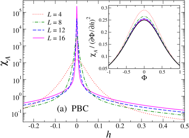
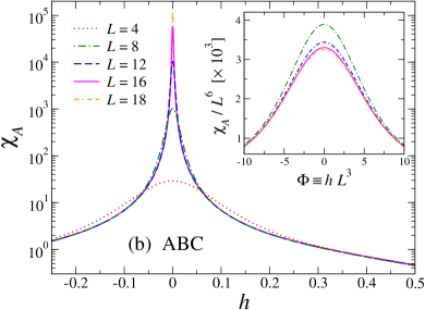
Figure 11: Fidelity susceptibility $\chi_{A}(L,h)$ for the quantum Ising ring (113) at fixed $g$, associated with changes of the longitudinal parameter $h$, for some values of $L$. Panel $(a)$ is for $g=0.9$ and $\zeta=1$ (PBC), for which one obtains the scaling variable $\Phi=2m_{0}hL/\Delta(L)$. Panel $(b)$ is for $g=0.5$ and $\zeta=-1$ (ABC), for which the scaling variable $\Phi=hL^{3}$ can be used. The two insets display curves for $\chi_{A}/(\partial\Phi/\partial h)^{2}$, which clearly approach a scaling function of $\Phi$. Note that curves in the inset of panel $(a)$ converge to the scaling function ${\cal A}_{2}(\Phi)$ (thick black line), cf. Eq. (159). Analogous results can be obtained for other values of $g<1$. Adapted from Ref. [382].

The scaling scenario of the fidelity and its susceptibility has been confirmed by analytical and numerical results for the $1d$ quantum Ising model across its FOQTs [382]. Figure 11, panel $(a)$, shows the fidelity susceptibility across the FOQT of systems with PBC, obtained by means of exact diagonalization and Lanczos algorithms. In this case, using the above correspondence, the scaling variable of Eq. (156) is given by $\Phi=2m_{0}hL/\Delta(L)$. The results nicely confirm the FSS at FOQTs reported in Eq. (158) and the scaling function (159) computed using the corresponding two-level model (105).

It is worth noting that the fidelity at FOQTs may also obey power-law behaviors when the BC give rise to domain walls in the ground state, such as ABC and OFBC. As discussed in Sec. 5.4, in such cases the gap behaves as $\Delta(L)\sim L^{-2}$, thus the scaling variable of Eq. (156) is expected to scale as $\Phi\approx hL^{3}$ and the scaling (158) of the fidelity susceptibility predicts that $\chi_{A}\sim L^{6}$. This implies

$$\widetilde{\chi}_{A}\sim L^{5}\,,$$ (160)

which is anyway a quite large power-law divergence. Expectations are well confirmed by the numerical results shown in Fig. 11, panel $(b)$. In such case, the scaling function is not the one reported in Eq. (159), since the two-level framework does not apply (see Sec. 5.4). 

We finally mention that the above FSS framework, both for CQTs and for FOQTs, can be generalized to a finite temperature $T$ [398, 37]. In such case, the quantum system is described by the density matrix

$$\rho_{w}\equiv\rho(L,T,w)=Z^{-1}\sum_{n}e^{-E_{n}/k_{B}T}|\Psi_{n}\rangle\langle\Psi_{n}|\,,\qquad Z=\sum_{n}\langle\Psi_{n}|e^{-E_{n}/k_{B}T}|\Psi_{n}\rangle\,.$$ (161)

One then needs Eq. (124) for the fidelity between mixed states,

$$A(L,T,w,\delta w)={\rm Tr}\left[\sqrt{\sqrt{\rho_{w}}\,\rho_{w+\delta w}\,\sqrt{\rho_{w}}}\right]\,,$$ (162)

which reduces to Eq. (144) for $T\to 0$. The corresponding fidelity susceptibility can be extracted analogously to Eq. (145). At a QT, the $T=0$ scaling (150) can be straightforwardly extended to keep into account the temperature, by adding a further scaling variable $\Xi=T/\Delta(L)$, cf. Eq. (97). For example, at CQTs, the corresponding susceptibility should asymptotically scale as

$$\widetilde{\chi}_{A}(L,T,w)\approx L^{\zeta}\,{\cal A}_{2}(\Xi,\Phi)\,,$$ (163)

when $\zeta>0$, cf. Eq. (152).

7.2 The bipartite entanglement entropy

In a quantum system, the reduced density matrices of subsystems, and, in particular, the corresponding entanglement entropies and spectra, provide effective probes of the nature of the quantum critical behavior (see, e.g., Refs. [453, 397, 454, 455, 456]). Their dependence on the finite size of the system may be exploited to determine the critical parameters of a QT [457, 458, 459, 460, 461, 462]. The spatial entanglement of systems near their QCP can be quantified by computing von Neumann or Rényi entanglement entropies of the reduced density matrix of a subsystem. They generally satisfy an area law, with some notable exceptions that present logarithmic corrections, such as free Fermi gases in arbitrary dimensions [463, 464, 455, 368, 465, 466], and 1$d$ many-body systems at CQTs described by 2$d$ CFT [467, 468, 469, 470, 454]. Recently, a protocol to measure the second-order Rényi entanglement entropy $S_{2}$ has been also experimentally implemented in a trapped-ion quantum simulator of spin chains [471].

7.2.1 Scaling behavior in one-dimensional continuous quantum transitions

We now discuss the scaling behavior of bipartite entanglement entropies of 1$d$ systems with a QCP characterized by $z=1$, thus realizing a CFT in two dimensions with central charge $c$. For example, one can consider $1d$ Ising-like quantum systems at their CQT for $g=g_{c}=1$, whose corresponding central charge is $c=1/2$. The lattice system can be divided into two connected parts $\tt{A}$ and $\tt{B}$ of length $\ell_{\tt A}$ and $\ell_{\tt B}=L-\ell_{\tt A}$. The reduced density matrix of subsystem $\tt{A}$ is given by $\rho_{\tt A}={\rm Tr}_{\tt B}\,\rho$, where $\rho$ is the density matrix of the ground state, and its corresponding von Neumann entropy is defined as

$$S(L,\ell_{\tt A};r,h)=S(L,L-\ell_{\tt A};r,h)=-{\rm Tr}\,[\rho_{\tt A}\log\rho_{\tt A}]\,.$$ (164)

The asymptotic behavior of bipartite entanglement entropies is known at the critical point $r=h=0$ [467, 468, 469, 470]:

$$S(L,\ell_{\tt A};r=0,h=0)\approx q\,{c\over 6}\Big{[}\log L+\log\sin(\pi\ell_{\tt A}/L)+e_{l}\Big{]}\,,$$ (165)

where $c$ is the central charge, $q$ counts the number of boundaries between the two parts of the system (thus $q=2$ for PBC, while $q=1$ for OBC), and $\log$ denotes the natural logarithm. The constant $e_{l}$ is nonuniversal and depends on the BC [469, 470, 472]. The asymptotic behavior of the bipartite entanglement entropies is also known in the thermodynamic limit close to the transition point [469, 473], i.e., for $L,\ell_{A}\ll\xi$, where $\xi$ is the length scale of the critical modes, such as that defined in Eq. (66). One obtains [469, 474, 473]

$$S(L,\ell_{\tt A};r,h=0)\approx q\,{c\over 6}\log\xi+e_{t}\,,\qquad\xi\ll\ell_{A},L\,,$$ (166)

where, again, $q=2$ for PBC and $q=1$ for OBC, and $e_{t}$ is a nonuniversal constant.

We now consider a critical system around its CQT point and consider the dependence on the relevant parameters $r$ and $h$ associated with the even and odd perturbations at the CQT, such as $r=g-1$ and $h$ entering the Hamiltonian (6) for the 1$d$ Ising chain. In the general FSS regime, using the notations of Sec. 4.2, the bipartite entanglement entropy has been conjectured to satisfy the asymptotic FSS [469, 475, 86, 476]

$$S(L,\ell_{\tt A};r,h)-S(L,\ell_{\tt A};r=0,h=0)\approx\Sigma(\ell_{\tt A}/L,L^{y_{r}}r,L^{y_{h}}h)\,,$$ (167)

so that $\Sigma(x,0,0)=0$. The corrections to this asymptotic behavior may have various origins [477, 473, 478, 479, 480, 460, 481, 482, 86]. Beside the FSS corrections discussed in the previous sections, such as the $O(L^{-\omega})$ corrections due to the leading irrelevant operator, the $O(L^{-1})$ corrections due to the presence of boundaries, and the $O(L^{-1/\nu})$ corrections arising from the $O(r^{2})$ terms of the scaling field $u_{r}\approx r$, there are additional corrections. They are related to the operators associated with the conical singularities at the boundaries between the two parts [477, 473]. In the limit $L,\ell_{\tt A}\to\infty$ at fixed $\ell_{\tt A}/L$, these new operators give rise to terms of order $L^{-y_{c}}$ in the case of OBC [477, 473] and of order $L^{-2y_{c}}$ in the case of PBC [479, 480]. Here $y_{c}>0$ is the RG dimension [477, 473] of the leading conical operator. This is conjectured to be essentially related to the energy operator [479, 480, 460, 482], hence $y_{c}=y_{r}$. Moreover, the analysis of exactly solvable models shows the presence of other corrections suppressed by integer powers of $L$ [479]. Analogous results apply to the $n$-index Rényi entropies, with the only difference that conical singularities lead to $O(L^{-y_{c}/n})$ corrections in the case of OBC [477, 473] and of order $L^{-2y_{c}/n}$ in the case of PBC [479, 480].

A thorough analysis of the FSS behavior of the von Neumann and Rényi entanglement entropies for the XY chain, confirming its asymptotic behavior (167) with the predicted corrections, is reported in Ref. [86].

We finally mention that a number of works has also focused on the entanglement spectrum, that is, the spectrum of the reduced density matrix $\rho_{\tt A}$ of subsystem ${\tt A}$. In particular, the behavior of the entanglement gap has been addressed in proximity of QCPs of various models (see, e.g., Refs. [483, 484, 461, 462, 485, 486, 487]).

7.2.2 Bipartite entanglement entropy in higher dimensions

In higher $d>1$ spatial dimensions, quantum spins or bosons develop an entanglement entropy that scales as the boundary of the bipartition [488, 489, 397, 455]. Some of the subleading contributions to the area law provide important sources of information for non-trivial quantum correlations, such as the topological entanglement entropy in a gapped spin-liquid phase [490, 491, 453, 456]. At a QCP, subleading terms contain information that identify the universality class (see, e.g., Refs. [492, 493, 494, 495, 496, 497, 498, 499, 500, 501, 502, 503, 504, 505]).

The leading contribution to $S_{\tt A}$, associated with a bipartition of 2$d$ systems of bosonic particle or spin systems, displays the area law

$$S_{\tt A}\approx b\,L_{\tt A}\,,$$ (168)

where $L_{\tt A}$ is the linear size of the boundaries between the two partitions, physically implying that the entanglement is local at the boundary of the partitions even at the critical point . The coefficient $b$ entering the area law (168) is sensitive to the short-distance cut-off, and is thus non-universal. Therefore, unlike 1$d$ cases, the leading behavior of the entanglement entropy in higher dimensions cannot be used to characterize the critical behavior. On the other hand, the subleading $O(1)$, or equivalently the leading part of the subtracted entanglement entropy

$$\Delta S_{\tt A}\equiv S_{\tt A}-b\,L_{\tt A}\,,$$ (169)

is expected to be universal in 2$d$ CQTs, thus providing information on the nature of the transition. Note that logarithmic behaviors of $\Delta S_{\tt A}$ may arise from corner contributions [506, 507], while they are expected to be absent for smooth boundaries between the partitions, where

$$\Delta S_{\tt A}\approx\gamma\,,$$ (170)

$\gamma$ being a universal constant. Computations at the Wilson-Fisher fixed point of O($N$) symmetry models, cf. Eq. (1), are reported in Refs. [505, 494], for various geometries, including those with sharp corners. Concerning the scaling properties of the bipartite entanglement entropy $S_{\tt A}$ around the QCP, we expect a behavior analogous to that reported in Eq. (167).

A strongly interacting quantum many-body system at zero temperature can exhibit exotic order beyond the LGW paradigm, dubbed topological order, whose defining property is that the ground-state degeneracy depends on the topology of the space. A class of models exhibiting these features is provided by 2$d$ spin-liquid models. Within these models, the concept of topological entanglement entropy has been proposed [456, 453], being proportional to the constant $\gamma$ entering Eq. (170), somehow replacing the role of the order parameter in a topologically ordered system. Based on the idea that the spin-liquid state is a type of collective paramagnet, the topological entanglement entropy probes long-distance correlations in the ground-state wave function that are not manifest as conventional long-range order. Some computations supporting the above ideas can be found, e.g., in Refs. [490, 491] within the paradigmatic toric code [508], a quantum dimer model on the triangular lattice [509], a BH on the Kagome lattice [510].

7.3 The concurrence between spins

Another aspect of the entanglement properties at CQTs is encoded into the entanglement between two spins in quantum spin models [397], such as the XY chain (7). In fact, the entanglement between two spin-1/2 systems has been investigated within the XY chain [511, 512]. This can be quantified through the concurrence, see Sec. 6.3.2. The two-spin concurrence turns out to vanish, unless the two sites are at most next-nearest neighbors, therefore it is somehow related to short-range quantum correlations. However, the concurrence $C_{\rm nn}$ between nearest-neighbor spins presents a critical behavior at the critical point $g_{c}=1$: its derivative with respect to the transverse-field parameter $g$ diverges logarithmically in the thermodynamic limit [512],

$$\partial_{g}C_{\rm nn}\approx{8\over 3\pi^{2}}\log|g-g_{c}|\,.$$ (171)

Thus, from the scaling point of view, the concurrence $C_{\rm nn}$ behaves as the first derivative of the free energy with respect to the relevant parameter $g$ (see, e.g., Ref. [86]), whose further derivative diverges logarithmically at the critical point (corresponding to the logarithmic divergence of the specific heat in the corresponding classical 2$d$ Ising model). A similar singular behavior is found also in the quantum discord of two close spins and other related quantities [513, 514, 515, 516, 37, 517, 518]. Results for other models have been also reported (see, e.g., Refs. [519, 520, 521, 522, 523, 524], the review article [397] and references therein). We mention that both the two-spin concurrence and the quantum discord are discontinuous at FOQTs [519, 520, 514].

8 Out-of-equilibrium dynamics at continuous quantum transitions

The recent progress that has been achieved in the control and manipulation of complex systems at the nano scale has enabled a wealth of possibilities to address the unitary quantum evolution of many-body objects [525, 526]. These range from the (nearly) adiabatic dynamics induced by a slow change in time of one of the control parameters, to the deep out-of-equilibrium dynamics following an abrupt quench.

The unitary dynamics across QTs can be induced by variations of the Hamiltonian parameters, which generally give rise to significant departures from adiabatic passages through equilibrium states. At both CQTs and FOQTs, a dynamic scaling behavior emerges when the out-of-equilibrium dynamics arises from sudden quenches of the Hamiltonian parameters, provided they remain within the critical regime, i.e., sufficiently close to the QT point [527]. It is worth stressing that at QTs the system is inevitably driven out of equilibrium, even when the time dependence is very slow, because large-scale modes are unable to equilibrate as the system changes phase. Off-equilibrium phenomena, as for example hysteresis and coarsening, Kibble-Zurek defect production, aging, etc., have been addressed in a variety of contexts, both experimentally and theoretically, at classical and quantum phase transitions (see, e.g., Refs. [528, 113, 529, 530, 531, 532, 533, 4, 5, 534, 535, 536, 188, 537] and references therein). These studies have shown that the time-dependent properties of systems evolving under such dynamics obey out-of-equilibrium scaling behaviors, depending on the universal static and dynamic exponents of the equilibrium QT [538, 539, 540, 541, 542, 543, 544, 390, 527].

The so-called quantum quench represents one of the simplest protocols in which a system can be naturally put in out-of-equilibrium conditions [221, 545, 546, 547, 548, 549], by suddenly changing a Hamiltonian parameter. Several interesting issues have been investigated in this context. They include the long-time relaxation and the consequent spreading of quantum correlations and entanglement, the statistics of the work, localization effects due to the mutual interplay of interactions and disorder, dynamical phase transitions, the dynamic scaling close to QTs, effects of dissipation or of measurements due to interactions with an environment, to mention some of the most representative ones (see, e.g., Refs. [550, 551, 552, 553, 554, 555, 556, 557, 558, 559, 560, 561, 562, 563, 564, 565, 566, 567, 568, 569, 570, 571, 572, 527, 573, 574, 575, 576, 545, 546, 577, 547, 548, 549, 578, 579, 580, 581, 582, 583, 584, 585, 586, 587, 588, 589, 590, 591]). All of them are eventually devoted to characterize the highly nonlinear response of the system to the drive, where nonequilibrium fluctuation relations may play a pivotal role [592, 593, 594, 595].

Several aspects related to the dynamics, and the asymptotic states, arising from quantum quenches have been intensely investigated and collected in a number of review articles, such as Refs. [10, 570, 17, 16, 19]. The asymptotic behavior of the quench dynamics in closed systems has been widely debated, in particular whether the large-time stationary states arising from unitary dynamics effectively behave as thermal states, thus leading to thermalization, and under which conditions. While the full density matrix can never show thermalization under unitary time evolution, the reduced density matrix related to sufficiently small subsystems can look effectively thermal, with the remaining (integrated out) system acting like an effective reservoir for it. The eigenstate thermalization hypothesis (ETH) has been argued to represent a key point to understand thermalization, assuming that the relevant energy eigenstates of a many-body Hamiltonian appear as thermal, i.e., that they are practically indistinguishable from equilibrium thermal states, as long as one focuses on macroscopic observables [596, 597, 598, 599, 556, 600, 601, 602, 603, 604, 605, 606, 607]. Other ideas have been also proposed to characterize the thermalization process in closed quantum systems, such as typicality [608, 609, 610] and quantum correlation effects [611, 612, 613].

Most quantum systems are expected to thermalize under a quench associated with an extensive energy interchange, however there are some notable exceptions, such as integrable systems [555, 614, 562, 563, 615] (see, e.g., Refs. [4, 16, 17, 18] for reviews on quantum quenches in integrable spin chains and quadratic Hamiltonians, also discussing the generalized Gibbs ensembles characterizing their asymptotic states), and systems showing many-body localization [616, 617, 618, 619, 620, 621, 622] (see Refs. [10, 11, 12, 13, 14, 15, 623] for reviews). We also mention the review article [570] focussing on quantum quenches in (1+1)-dimensional CFTs [624, 625, 626]. Another related and interesting issue concerns the evidence of peculiar dynamical phase transitions and prethermalization after quenches of O($N$) and other models [627, 628, 629, 630, 569, 631, 632, 633, 634]. We will not pursue the above-mentioned issues further, for which we refer to the literature cited therein.

To stay within the focus of this review, in the following we discuss issues closely related to the presence of CQTs (FOQTs are addressed in Sec. 10). We primarily consider sudden soft quenches probing the critical modes associated with equilibrium QTs, thus involving sufficiently low energies to excite only long-range critical fluctuations. We characterize the scaling behaviors of the out-of-equilibrium unitary dynamics at QTs arising from soft quenches. As an exception, in Sec. 8.7 we also discuss hard quenches to QCPs, reporting results that somehow signal the presence of QCP, in particular in integrable systems, even though the energy associated with the quench is relatively large. The out-of-equilibrium dynamics arising from slow changes of the Hamiltonian parameters across QTs will be discussed in the forthcoming section 9.

In the following we only consider homogeneous global quenches. We mention that also local quenches have been studied in the literature (see, e.g., Refs. [635, 626, 636, 637, 638]), for example to address issues related to the spread of the quantum information after a sudden local change of the system [639, 640, 641].

8.1 Quench protocols

A dynamic quench protocol is generally performed within a family of Hamiltonians, that are written as the sum of two noncommuting terms:

$$\hat{H}(w)=\hat{H}_{c}+w\hat{H}_{p}\,,$$ (172)

where $\hat{H}_{c}$ and $\hat{H}_{p}$ are independent of the parameter $w$, and $[\hat{H}_{c},\hat{H}_{p}]\neq 0$.  The tunable parameter $w$ enables to modify the strength of the perturbation $\hat{H}_{p}$, e.g., a magnetic-field term in a system of interacting spins, with respect to the unperturbed Hamiltonian $\hat{H}_{c}$. In the following we assume that $\hat{H}_{c}$ represents a critical Hamiltonian, such as the quantum Ising model (6) at $g=g_{c}$ and $h=0$, while $w$ is a relevant parameter driving the QT. Thus, $w$ may correspond to the transverse (t) field $r=g-g_{c}$ or the longitudinal (l) field $h$, associated with the transverse and longitudinal spin terms $\hat{H}_{p,{\rm t}}=-\sum_{\bm{x}}\hat{\sigma}_{\bm{x}}^{(3)}$ and $\hat{H}_{p,{\rm l}}=-\sum_{\bm{x}}\hat{\sigma}_{\bm{x}}^{(1)}$, respectively. The critical point corresponds to $w=w_{c}=0$.

A quantum quench protocol is performed as follows:

• The system is prepared in the ground state of the Hamiltonian (172) associated with an initial value $w_{i}$, that is, at $t=0$ the system starts from $|\Psi(t=0)\rangle\equiv|\Psi_{0}(w_{i})\rangle$. Alternatively, one may consider an initial state at temperature $T$, described by the Gibbs distribution $\rho_{0}(w_{i})\propto\exp[-\hat{H}(w_{i})/T]$.

• Then the Hamiltonian parameter is suddenly changed to $w\neq w_{i}$. The resulting dynamic problem corresponds to that of the unitary quantum evolution driven by the Hamiltonian $\hat{H}(w)$, i.e.,

  $$|\Psi(t)\rangle=e^{-i\hat{H}(w)t}|\Psi(0)\rangle\,,\qquad\qquad|\Psi(0)\rangle\equiv|\Psi_{0}(w_{i})\rangle\,.$$ (173)

The out-of-equilibrium evolution of the system can be investigated by monitoring observables and correlations obtained by taking expectation values at fixed time. For example, in the case of lattice spin models, one may consider the longitudinal magnetization, the two-point function of local operators related to the order parameter, etc. In particular, for quantum Ising models (see Sec. 3.1), one may consider the evolution of the local and global average magnetization

$$m_{\bm{x}}(t)\equiv\big{\langle}\hat{\sigma}_{\bm{x}}^{(1)}\big{\rangle}_{t}\,,\qquad M(t)\equiv L^{-d}\sum_{\bm{x}}m_{\bm{x}}(t)\,,$$ (174)

as well as the fixed-time correlation function of the order-parameter operator and its space integral,

$$G(t,{\bm{x}}_{1},{\bm{x}}_{2})\equiv\big{\langle}\hat{\sigma}_{{\bm{x}}_{1}}^{(1)}\,\hat{\sigma}_{{\bm{x}}_{2}}^{(1)}\big{\rangle}_{t}\,,\qquad\chi(t,{\bm{x}}_{0})=\sum_{\bm{x}}G({t,\bm{x}}_{0},{\bm{x}})\,,$$ (175)

together with their connected contribution,

$$G_{c}(t,{\bm{x}}_{1},{\bm{x}}_{2})\equiv G(t,{\bm{x}}_{1},{\bm{x}}_{2})-m_{{\bm{x}}_{1}}(t)\>m_{{\bm{x}}_{2}}(t)\,.$$ (176)

In the above formulas (174) and (175), $\langle\,\hat{O}\,\rangle_{t}$ denotes the expectation value of the operator $\hat{O}$ at time $t$. In the case the system is in a pure state $|\Psi(t)\rangle$, as for the quench protocol following Eq. (173), this is given by $\langle\hat{O}\rangle_{t}\equiv\langle\Psi(t)|\hat{O}|\Psi(t)\rangle$. In the case the system is in a mixed state $\rho(t)$, as when starting at finite temperature or in the presence of dissipation (see Sec. 13), this is given by $\langle\hat{O}\rangle_{t}\equiv{\rm Tr}\,\big{[}\hat{O}\,\rho(t)\big{]}$.

In the following, we distinguish between soft and hard quenches around or to QTs. Their difference is essentially related to the extension of the energy levels they involve in the post-quench dynamics. Soft quenches are related to changes of the Hamiltonian parameters whose initial and final values stay close to the QT point, thus only exciting the low-energy critical modes. As we shall see, soft quenches can be effectively described by dynamic scaling frameworks, within which the validity of the soft-quench regime can be quantitatively addressed. On the other hand, the more general hard quenches are not limited by the above criticality condition. For example they occur when the initial values of the Hamiltonian parameters are far from the QT point, thus the post-quench dynamics also involves high-energy levels that are not critical at QTs. In this case, the resulting out-of-equilibrium dynamics is not generally expected to develop scaling behaviors.

8.2 Homogeneous scaling laws for the out-of-equilibrium dynamics

As largely discussed in the literature, the unitary dynamics of closed systems at CQTs develops dynamic scaling laws (see, e.g., Refs. [539, 543, 540, 642, 541, 542, 643, 644, 527, 390, 537, 570, 645, 573, 646, 647, 648, 649, 650]). In the following we discuss the conditions in which dynamic scaling laws emerge from out-of-equilibrium regimes, and their main features. We focus on the quantum dynamics arising from instantaneous quenches of closed systems at CQTs, described by the Hamiltonian (172).

As a working hypothesis, we assume homogeneous scaling laws that extend those holding at equilibrium (see Sec. 4), such as that reported in Eq. (52). The main point of such extension to the out-of-equilibrium dynamics is that the time dependence of observables in the dynamic scaling limit is obtained through the dependence of the scaling functions on a scaling variable associated with time,

$$\Theta\sim\Delta\,t\,,$$ (177)

which is obtained by assuming that the relevant time scale of the critical modes is proportional to the inverse energy difference $\Delta$ of the lowest states. This can be implemented by adding a dependence on $b^{-z}t$ in the scaling functions of the homogeneous scaling laws, where $z$ is the critical exponent controlling the suppression of the gap at the critical point. Therefore, the evolution of a generic observable $O$, such as the expectation value at time $t$ of a local operator $\hat{O}$, is expected to asymptotically satisfy the homogeneous scaling relation 

$$O(t;L,w_{i},w)\equiv\big{\langle}\hat{O}\big{\rangle}_{t}\approx b^{-y_{o}}\,{\cal O}(b^{-z}t,b^{-1}L,b^{y_{w}}w_{i},b^{y_{w}}w)\,,$$ (178a)

where $$b y_{o} \hat{O} y_{w} w L {\cal O} b$$ is an arbitrary positive parameter, is the RG dimension of the operator , is the RG dimension of the Hamiltonian parameter , is the size of the system, and is a universal scaling function apart from normalizations, see Sec. 4.3. Equation (178a) is expected to provide the asymptotic power-law behavior in the large- limit.

Analogously, in the case of fixed-time correlation functions of two generic local operators $\hat{O}_{1}$ and $\hat{O}_{2}$, two-point correlation functions only depend on the difference ${\bm{x}}\equiv{\bm{x}}_{2}-{\bm{x}}_{1}^{~{}\ref{eq:notequench1}}$. Their dynamic scaling is thus expected to satisfy the homogeneous law

$$G_{12}(t,{\bm{x}};L,w_{i},w)\equiv\big{\langle}\hat{O}_{1}({\bm{x}}_{1})\,\hat{O}_{2}({\bm{x}}_{2})\big{\rangle}_{t}\approx b^{-\varphi_{12}}\,{\cal G}_{12}(b^{-z}t,b^{-1}{\bm{x}},b^{-1}L,b^{y_{w}}w_{i},b^{y_{w}}w)\,,$$ (178b)

where $\varphi_{12}=y_{1}+y_{2}$ and $y_{j}$ are the RG dimensions of the operators $\hat{O}_{j}$. 

To simplify the presentation, in the dynamic homogeneous scaling laws (178b) we have not inserted the scaling fields within the arguments of the scaling functions ${\cal O}$ and ${\cal G}_{12}$, as was done in Sec. 4, but we have only reported their leading approximation in terms of the Hamiltonian parameters. The asymptotic behavior is not changed; the differences arise at the level of some typically subleading scaling corrections, which will be neglected in the following.

The dynamic scaling framework can be extended to situations where the initial condition is given by a Gibbs ensemble at temperature $T$, by adding a further dependence on the product $b^{z}T$ in the scaling functions of Eqs. (178b).

We finally note that the above dynamic scaling behaviors, and in particular the scaling of the time dependence, is analogous to that arising in the critical dynamics of classical systems, within RG frameworks [528, 531]. We recall that the exponent $z$ of the critical dynamics at classical phase transitions is a further independent critical exponent that also depends on the type of dynamics considered [528]. In quantum many-body systems, the time dependence arises from the unitary quantum dynamics, therefore the time dependence of the corresponding critical dynamics is controlled by the same dynamic exponent $z$ describing the suppression of the energy difference of the lowest states at the transition point.

8.3 Dynamic scaling arising from soft quenches at quantum transitions

8.3.1 General scaling behaviors

The dynamic scaling in the infinite-volume thermodynamic limit can be straightforwardly obtained from the scaling laws (178b), by setting

$$b=\lambda\equiv|w|^{-1/y_{w}}\,,$$ (179)

and taking the limit $L/\lambda\to\infty$ (of course this limit is meaningless at strictly $w=0$). Assuming that such limit is well defined, one obtains

$$O(t;w_{i},w)\,\approx\; \lambda^{-y_{o}}\,{\cal O}_{\infty}(\lambda^{-z}t,\lambda^{y_{w}}w_{i})\,,$$ (180a)

$$G_{12}(t,{\bm{x}};w_{i},w)\,\approx\; \lambda^{-\varphi_{12}}\,{\cal G}_{\infty}(\lambda^{-z}t,\lambda^{-1}{\bm{x}},\lambda^{y_{w}}w_{i})\,.$$ (180b)

We should emphasize that the above dynamic scaling limit requires that the pre- and post-quench Hamiltonians remain in the critical regime of a QT, i.e., $w_{i}$ and $w$ are sufficiently small.

The asymptotic dynamics scaling allowing for the finite size $L$ of the system can be obtained from the same scaling laws (178b), by simply setting $b=L$, while the parameter $w$ may take any value, including $w=0$. The resulting scaling ansatze can be written as

$$O(t;L,w_{i},w)\,\approx\; L^{-y_{o}}\,{\cal O}(L^{-z}t,w_{i}/w,L^{y_{w}}w)\,,$$ (181a)

$$G_{12}(t,{\bm{x}};L,w_{i},w)\,\approx\; L^{-\varphi_{12}}\,{\cal G}_{12}(L^{-z}t,L^{-1}{\bm{x}},w_{i}/w,L^{y_{w}}w)\,.$$ (181b)

Therefore, an asymptotic dynamic FSS is expected to emerge in the large-$L$ and large-time limit, keeping the scaling variables

$$\Theta=L^{-z}\,t\,,\qquad{\bm{X}}=\frac{\bm{x}}{L}\,,\qquad\Phi_{i}=L^{y_{w}}\,w_{i}\,,\qquad\Phi=L^{y_{w}}\,w\,,\qquad\delta_{w}=\frac{w}{w_{i}}-1\,,$$ (182)

fixed . It is also possible to include the effect of a small finite temperature, assuming a Gibbs ensemble as initial condition, by adding the scaling variable $\Xi=L^{z}\,T$ as a further argument of the dynamic FSS functions (181).

The above considerations provide the appropriate conditions under which we may observe dynamic scaling corresponding to the soft-quench scaling regime. This is obtained by keeping the scaling variables (182) fixed in the large-size limit, thus we need to tune the Hamiltonian parameters so that they stay close to the QTs, according to $w_{i}\sim w\sim L^{-y_{w}}$, which is the condition to ensure that only the low-energy critical modes effectively get excited during the post-quench dynamics, for $t\sim L^{z}$. Moreover the asymptotic dynamic FSS, keeping the scaling variables (182) fixed, is expected to be approached with power-law suppressed corrections, analogously to the approach to the asymptotic equilibrium FSS discussed in Sec. 4.

A similar dynamic scaling behavior has been also put forward in the context of trapped bosonic gases [306], extending the equilibrium TSS discussed in Sec. 4.6 to a dynamical TSS. This can be obtained by replacing $L$ with $\ell^{\theta}$ in the dynamic FSS equations [we recall that $\ell$ is the trap size, cf. Eq. (81), and $\theta\leq 1$ is the trap exponent, cf. Eq. (90)].

A related important issue regards the thermalization, that is, whether the system presents a local thermal-like behavior at an asymptotically long time after the quench. Understanding under which circumstances this occurs is a highly debated issue [5, 6, 7, 8, 9, 10], being related to the integrability properties of the Hamiltonian $\hat{H}_{c}$, the mutual interplay of interactions and inhomogeneities, and the nature of the spectrum. An effective thermalization may emerge in the large-volume limit (of nonintegrable systems), keeping the parameters $w\neq w_{i}$ fixed, i.e., in the limit $\Phi\to\infty$, when the quench protocol entails energy interchanges growing as the volume. However, in this hard-quench regime also noncritical modes get excited, therefore the dynamics is expected to lose the typical features of the critical dynamics. We will return to this point in Sec. 8.7.

8.3.2 Quantum quenches at the continuous transition of the Ising chain

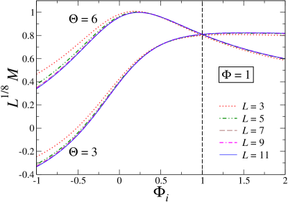
Figure 12: Magnetization for fixed $\Phi=1$ and for two different rescaled times $\Theta$. The curves are plotted against the rescaled parameter $\Phi_{i}$, which is used to compute the initial state. Notice that, at $\Phi_{i}=\Phi=1$, the equilibrium behavior is recovered (vertical dashed line). The curves at different size appear to approach an asymptotic function, in accordance with the dynamic FSS theory. Adapted from Ref. [527].

The above dynamic scaling ansatze have been confirmed by numerical studies within the 1$d$ Ising chain (6) at its CQT point $g_{c}=1$ and $h=0$. In particular, let us consider the case in which the instantaneous quench is performed on the longitudinal field $h$, keeping $g=g_{c}$ fixed. Specializing to the Ising chain, the magnetization $M$ and the two-point connected correlation function $G_{c}$ of the order-parameter field, cf. Eqs. (174)-(176), show the asymptotic dynamic FSS behaviors:

$$M(t;L,w_{i},w)\approx L^{-\beta/\nu}\,{\cal M}(\Theta,\Phi_{i},\Phi)\,,\qquad G_{c}(t,x;L,w_{i},w)\approx L^{-\eta/\nu}\,{\cal G}(\Theta,X,\Phi_{i},\Phi)\,,$$ (183)

where we assumed translation invariance, $\beta=1/8$ denotes the magnetization critical exponent, $\nu=1$ and $\eta=1/4$, and thus $\beta/\nu=1/8$ and $\eta/\nu=1/4$. This out-of-equilibrium FSS behavior has been checked by numerical computations based on exact diagonalization [527]. As an example, Fig. 12 displays the magnetization after a quench at fixed rescaled time $\Theta$ and $\Phi=1$, as a function of $\Phi_{i}$. The various curves spotlight the emergence of a scaling behavior. Further results can be found in the original work [527].

8.4 Scaling behavior of the Loschmidt echo

The Loschmidt amplitude quantifies the deviation of the post-quench state at time $t>0$ from the initial state before the quench, and is strictly connected with the concept of the fidelity (see Sec. 6.1). It is defined as the overlap

$$\widetilde{A}(t)=\langle\Psi_{0}(w_{i})|\Psi(t)\rangle=\langle\Psi_{0}(w_{i})|e^{-i\hat{H}(w)t}|\Psi_{0}(w_{i})\rangle\,.~{}$$ (184)

The so-called Loschmidt echo $Q(t)$ is identified with its rate function,

$$Q(t)=-\ln\big{|}\widetilde{A}(t)\big{|}^{2}\,.$$ (185)

Note that $Q(t)=0$ implies the restoration of the initial quantum state.

The dynamic scaling behavior of $Q(t)$ at QTs was addressed in Ref. [527], focusing on quenches of the longitudinal field $h$ in quantum Ising models, thus $w\equiv h$, and numerically investigating it within 1$d$ systems. Its time dependence after the quench is conjectured to obey the dynamic FSS behavior

$$Q(t;L,w_{i},w)\approx{\cal Q}(\Theta,\Phi,\delta_{w})\,.$$ (186)

An illustrative example is reported in Fig. 13, which shows that the numerical data fully support the dynamic FSS predicted by the scaling equation (186). The emerging pattern is similar to that of the magnetization. We also note the presence of quasi-complete revivals of the quantum states along the quantum evolution, when $Q(t)\ll 1$.

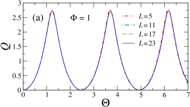
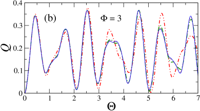
Figure 13: Temporal behavior of the Loschmidt echo $Q(t)$ defined in Eq. (185) for $\delta_{w}=-2$, and two different values of $\Phi=1$ ($a$) and $\Phi=3$ ($b$). Data are plotted against the rescaled time $\Theta=L^{-z}\,t$, so that the convergence to a scaling function, in the large-$L$ limit, is clearly visible. Adapted from Ref. [527].

8.5 Scaling properties of work fluctuations after quenches near quantum transitions

We now address issues related to the statistics of the work done on a many-body system close to a QT, when this is driven out of equilibrium by suddenly switching one of the control parameters [594, 651], such as the quenching protocol described in Sec. 8.1. Several issues related to this topic have been already discussed in a variety of physical implementations, including spin chains [652, 653, 654, 655, 656, 657, 658, 659], fermionic and bosonic systems [660, 561, 661, 662], quantum field theories [663, 664, 665, 666], as well as in different contexts like cyclically driven systems [667] and dynamic quantum phase transitions [566]. It has also been shown that the work statistics can be experimentally measured in present-day ultracold-atom systems, by means of ion traps [668] or Ramsey interferometry [669, 670].

The research done so far in this context has mostly addressed the thermodynamic limit of systems close to criticality (see, e.g., Ref. [651] and references therein). However, it is phenomenologically important to know the impact of having a finite size, in order to achieve a deep understanding of any reliable quantum-simulation experiment. Indeed, for a global quench the work is extensive. Therefore in the thermodynamic (i.e., large-volume) limit, keeping the Hamiltonian parameter fixed, one expects the probability associated with the work density $W/V$ (where $V=L^{d}$ is the volume of the system) to be sharply peaked around its average value, with typical fluctuations suppressed as $V^{-1/2}$. The work distribution is expected to approach a quasi-Gaussian distribution in the infinite volume limit, around the average value of the work density $W/L^{d}$. One also expects $O(L^{-d/2})$ fluctuations having the general form $P(W)\sim\exp[-L^{d}I(W/L^{d})]$, with $I(x)\geq 0$ [561, 651]. This suggests that fluctuations around the work average, and in particular deviations from Gaussian behaviors, may be only observable for relatively small systems.

8.5.1 Work fluctuations associated with a quench

The quantum work $W$ associated with a quench protocol, i.e., the work done on the system by quenching the control parameter $w$, does not generally have a definite value. More specifically, this quantity can be defined as the difference of two projective energy measurements [594]. The first one, at $t=0$, projects onto the eigenstates of the initial Hamiltonian $\hat{H}(w_{i})$ with a probability given by the equilibrium Gibbs distribution. Then the system is driven by the unitary operator $e^{-i\hat{H}(w)t}$ and the second energy measurement projects onto the eigenstates of the post-quench Hamiltonian $\hat{H}(w)$. The work probability distribution can thus be written as [594, 671, 672]

$$P(W)=\sum_{n,m}\delta\big{\{}W-[E_{n}(w)-E_{m}(w_{i})]\big{\}}\,\big{|}\langle\Psi_{n}(w)|\Psi_{m}(w_{i})\rangle\big{|}^{2}\,p_{m}\,,\quad$$ (187)

where $\{E_{n}(w)\}$ and $\{|\Psi_{n}(w)\rangle\}$ denote eigenvalues and eigenstates of the Hamiltonian $\hat{H}(w)$, and $p_{m}$ are the probabilities of the initial eigenstates $|\Psi_{m}(w_{i})\rangle$. For example, in the case of an initial Gibbs distribution with temperature $T$, one has $p_{m}\propto\exp[-E_{m}(w_{i})/T]$. One may also introduce a corresponding characteristic function [652, 594]

$$C(s)=\int dW\,e^{isW}\,P(W),$$ (188)

encoding full information of the work statistics.

The work distribution (187) satisfies the quantum version of the Crooks fluctuation relation [594]

$$\frac{P(W,T,w_{i},w)}{P(-W,T,w_{i},w)}=e^{W/T}e^{-\Delta F/T}\,,\qquad\Delta F=F(w)-F(w_{i})\,,$$ (189)

where the probability distribution in the denominator corresponds to an inverted quench protocol, from $w$ to $w_{i}$, and where $F=-T\,\ln Z$ is the free energy. It also satisfies the Jarzynski equality [593, 594]:

$$\langle e^{-W/T}\rangle\equiv\int dW\,e^{-W/T}\,P(W)=e^{-\Delta F/T}\,.$$ (190)

One may also define the so-called dissipative work [594] $W_{d}=W-\Delta F$, satisfying the inequality $\langle W_{d}\rangle\geq 0$.

The zero-temperature limit corresponds to a quench protocol starting from the ground state $|\Psi_{0}(w_{i})\rangle$ of $\hat{H}(w_{i})$. Assuming that such ground state is nondegenerate, the work probability (187) reduces to

$$P(W)=\sum_{n}\delta\big{\{}W-[E_{n}(w)-E_{0}(w_{i})]\big{\}}\,\big{|}\langle\Psi_{n}(w)|\Psi_{0}(w_{i})\rangle\big{|}^{2}\,.$$ (191)

In this case, the dissipative work simplifies to $W_{d}=W-[E_{0}(w)-E_{0}(w_{i})]$, and the characteristic function $C(s)$ can be simply written as the amplitude

$$C(s)=\langle\Psi_{0}(w_{i})|e^{-i\hat{H}(w_{i})s}\,e^{i\hat{H}(w)s}|\Psi_{0}(w_{i})\rangle\,,$$ (192)

whose absolute value is related the Loschmidt echo $Q(t)=-\ln|\langle\Psi_{0}(w_{i})|\Psi(t)\rangle|^{2}$, providing information on the overlap between the initial state $|\Psi_{0}(w_{i})\rangle$ and the evolved quantum state $|\Psi(t)\rangle$ at time $t$.

8.5.2 Scaling of the work fluctuations

We now discuss the behavior of such quantities at CQTs. To this purpose, we distinguish two cases:

• the case in which $w$ is an odd Hamiltonian parameter, such as the longitudinal field $h$ in quantum Ising models, thus correspondingly $\langle\hat{H}_{p}\rangle=0$ at the critical point $w=0$;

• the case in which $w$ is an even Hamiltonian parameter, such as the transverse field $g$ in quantum Ising models (more precisely $w=r=g-g_{c}$), thus $\langle\hat{H}_{p}\rangle\neq 0$ at the critical point $w=0$.

In case (i) work fluctuations develop notable scaling behaviors, while in case (ii) things get more complicated.

Assuming the existence of a nontrivial dynamic FSS limit for the work distribution $P(W)$, as expected for the case (i), a natural working hypothesis is that it is defined as the large-size limit keeping the appropriate scaling variables fixed, such as [573]

$$P(W,L,w_{i},w)\approx\Delta(L)^{-1}\>{\cal P}(\Omega,\Phi,\delta_{w})\,,\qquad\Omega\equiv{W\over\Delta(L)}\,,$$ (193)

in the zero-temperature limit, where $\Delta(L)$ is the energy gap of the lowest states at $w=0$, and we have introduced a further scaling variable $\Omega$. The dynamic FSS limit is defined as the large-size $L\to\infty$ limit, keeping $\Omega$, $\Phi$, and $\delta_{w}=w/w_{i}-1=\Phi/\Phi_{i}-1$ fixed. The dynamic FSS (193) allows us to infer the scaling behavior of the average of the work and its higher moments $\langle W^{k}\rangle\equiv\int dW\,W^{k}\,P(W)$, as well. Equation (193) also determines the scaling behaviors of the corresponding characteristic function (188),

$$C(s;L,w_{i},w)\approx{\cal C}(\Theta_{s},\Phi,\delta_{w})\,,\qquad\Theta_{s}\equiv L^{-z}\,s\,.$$ (194)

The above formulas can be straightforwardly extended to allow for a finite temperature $T$ of the initial state.

Using the general dynamic FSS of the work probability, one can derive the corresponding behavior of the zero-temperature average work, i.e., $\langle W\rangle=\Delta(L)\,{\cal W}_{1}(\Phi_{i},\Phi)$. Actually, the same scaling behavior can be equivalently derived by noting that

$$\langle W\rangle=\langle\Psi_{0}(w_{i})|\hat{H}(w)-\hat{H}(w_{i})|\Psi_{0}(w_{i})\rangle=(w-w_{i})\langle\Psi_{0}(w_{i})|\hat{H}_{p}|\Psi_{0}(w_{i})\rangle\approx L^{d-y_{p}}\,\delta_{w}w_{i}\,f_{p}(\Phi_{i})\,,$$ (195)

where $y_{p}$ and $f_{p}$ are, respectively, the RG dimension and the equilibrium FSS function associated with the observable $\hat{H}_{p}/L^{d}$. Then, taking into account the hyperscaling relation $y_{p}+y_{w}=d+z$ between the RG dimensions of $w$ and of the associated perturbation $\hat{H}_{p}$ [1, 86], we have that

$$\langle W\rangle\approx L^{-z}{\cal W}_{1}(\Phi_{i},\Phi)\,,\qquad{\cal W}_{1}(\Phi_{i},\Phi)\sim\delta_{w}\,\Phi_{i}\,f_{p}(\Phi_{i})\,,\qquad\delta_{w}={w\over w_{i}}-1\,,$$ (196)

in agreement with the scaling behavior of the average work $\langle W\rangle=\int dW\,W\,P(W)$ that is obtained using the scaling ansatz (193). This provides a relation between the dynamic FSS function of the average work and the equilibrium FSS function of the expectation value of the Hamiltonian term $\hat{H}_{p}$ associated with the driving parameter $w$. Taking the large-volume limit ($L\to\infty$) of the above scaling behaviors, the average work is expected to grow as the volume, which implies

$$f_{p}(\Phi_{i})\sim|\Phi_{i}|^{y_{p}/y_{w}},\qquad|\Phi_{i}|\to\infty,\qquad\langle W\rangle\sim L^{d}\,(w-w_{i})\,|w_{i}|^{y_{p}/y_{w}}\,.$$ (197)

This can be also written as

$${\langle W\rangle/L^{d}}\sim\delta_{w}\,\xi_{i}^{-(d+z)}\,,\qquad\xi_{i}\sim|w_{i}|^{-1/y_{w}}\,,$$ (198)

where $\xi_{i}$ represents an infinite-volume correlation length associated with the initial ground state of $\hat{H}(w_{i})$.

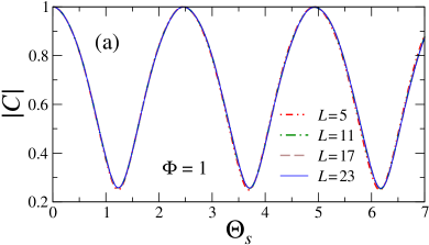
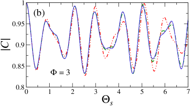
Figure 14: Scaling of the modulus of the characteristic function $|C(s)|$ associated to a quench of the Ising model for $\delta_{w}=-2$. The two panels refer to $\Phi=1$ ($a$) and $\Phi=3$ ($b$). Data are plotted against the rescaled time $\Theta_{s}=L^{-z}\,s$, so that the convergence to a scaling function, in the large-$L$ limit, is clearly visible. Adapted from Ref. [573].

As already mentioned, the above scaling behaviors of the work fluctuations are expected to apply when the driving parameter is odd [case (i)], i.e., when the expectation value of $\hat{H}_{p}$ vanishes on the ground state of the critical Hamiltonian (for $w=0$). This is demonstrated by the data in Fig. 14 for the characteristic work function, cf. Eq. (188), of the 1$d$ Ising chain, associated with a quench of the longitudinal field $h$: they clearly support the scaling behavior put forward in Eq. (194). In contrast, as discussed in Ref. [673], when the driving parameter is associated with an even perturbation [case (ii)], such as for $w=r=g-g_{c}$ in the quantum Ising models, then work fluctuations get dominated by analytical terms (mixing with the identity operator), while the scaling terms remain subleading.

We finally mention that the behavior of work fluctuations arising from soft quenches has been also investigated within the BH model in the hard-core limit, driven by an external constant field globally coupled to the bosonic modes, through the vacuum-to-superfluid CQT, extending the analysis to particle systems confined by inhomogeneous external potentials [573].

8.6 Scaling of the bipartite entanglement entropy after soft quenches

The time evolution of the entanglement entropy of bipartitions $\tt{A}|\tt{B}$ of the system, cf. Eq. (164), quantifies the amount of quantum correlations that are present between the two parts of the chain after soft quenches around a CQT.  Here we focus on 1$d$ quantum spin systems, such as Ising-like chains, and consider a bipartition into two parts of size $\ell_{\tt A}$ and $L-\ell_{\tt A}$. Extending equilibrium scaling arguments (see, Sec. 7.2), the following dynamic FSS behavior has been conjectured for its behavior after quenches from $w_{i}$ to $w$ [527]

$$\Delta S(t;L,\ell_{\tt A};w_{i},w)\equiv S(t;L,\ell_{\tt A};w_{i},w)-S_{c}(L,\ell_{\tt A})\approx{\cal S}(\Theta,\ell_{\tt A}/L,\Phi,\delta_{w})\,,$$ (199)

where $S_{c}(L,\ell_{\tt A})$ accounts for the critical FSS behavior (165). Numerical checks within the Ising chain [527] support this asymptotic scaling behavior, as shown in Fig. 15, with corrections generally decaying as $1/L$.

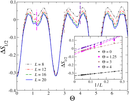
Figure 15: Temporal behavior of the entanglement entropy $\Delta S_{1/2}\equiv\Delta S(t;L,L/2;w_{i},w)$ for a balanced bipartition in a quantum Ising ring, after quenching the longitudinal field $h=w$ from $w_{i}=0$. The inset displays the convergence with $L$ of the various curves (up to $L=22$), for four values of $\Theta$ (see the long-dash lines in the main panel), plotted against $1/L$. Black stars denote data corresponding to the equilibrium condition $\Theta=0$. Dashed lines are numerical fits of the data at the largest available $L$. Adapted from Ref. [527].

8.7 Out-of-equilibrium dynamics after hard quenches to quantum critical points

As discussed in the previous subsections, the out-of-equilibrium dynamics arising from quantum quenches at CQTs develops scaling behaviors controlled by their universality class. These require the Hamiltonian parameters associated with the quench protocol, $w_{i}$ and $w$, to be close to the QCP, at $w=0$. However, in the case of hard quenches across the CQT (i.e., when $w_{i}$ and $w$ differ significantly), a dynamic scaling controlled by the universality class of the equilibrium QT is generally not expected, essentially because the instantaneous change of the Hamiltonian parameters entails a significant amount of energy exchange. Indeed, the instantaneous change from $w_{i}$ to $w$ gives rise to a relatively large amount $\Delta E$ of energy above the ground level of the Hamiltonian $\hat{H}(w)$,

$$\Delta E=\sum_{n}\big{[}E_{n}(w)-E_{0}(w)\big{]}\,\big{|}\langle\Psi_{n}(w)|\Psi_{0}(w_{i})\rangle\big{|}^{2}\sim L^{d}\,,$$ (200)

Typically $\Delta E$ is much larger than the energy scale $E_{c}$ of the low-energy excitations at criticality $w=0$, which is given by $E_{c}\sim L^{-z}$ with $z=1$ for CQTs of Ising-like systems. This would naturally lead to the expectation that the unitary energy-conserving dynamics, after quenching to the QCP, is not significantly related to the quantum critical features of the low-energy spectrum of the critical Hamiltonian. However, as argued in Refs. [677, 678, 679, 680, 681, 576], some signatures may emerge as well. In particular, integrable many-body systems (such as those mappable into generic noninteracting fermionic systems) develop peculiar discontinuities even in the asymptotic stationary states arising from the quantum quenches [677, 678, 576]. On the other hand, local observables are not expected to present singularities in nonintegrable systems where generic quantum quenches lead to thermalization, since they are generally smooth functions of the temperature (exceptions to this general behavior are seen to emerge in integrable models and in the presence of localization phenomena). Nonetheless, it has been recently argued that it is possible to recover signals from intermediate regimes of the post-quench quantum evolution [681].

8.7.1 Singular behavior of the XY chain

The above issue related to hard quenches has been thoroughly investigated within the quantum XY model (7), under quenches of the Hamiltonian parameter $g$ driving the transition that separates the quantum paramagnetic and ferromagnetic phases [562, 563, 677, 16, 576], starting from the ground states associated with initial values $g_{i}$. In the thermodynamic limit, the out-of-equilibrium evolution of the energy density [677], and the longitudinal and transverse magnetizations [576], develop a singular dependence on the quench parameter $g$, or $w\equiv g-g_{c}$, around the critical value $g=g_{c}$, for any anisotropy parameter $\gamma>0$ and starting point $g_{i}$, including the extremal ones corresponding to fully disordered and ordered initial states.

The behavior of the transverse (t) magnetization of the XY chain after a quench from $g_{i}$ to $g$,

$$M_{\rm t}(t)\equiv L^{-1}\sum_{x}m_{{\rm t},x}(t)\,,\qquad m_{{\rm t},x}(t)=\big{\langle}\hat{\sigma}^{(3)}_{x}\big{\rangle}_{t}\,,$$ (201)

has been analytically computed in the infinite-volume limit [550, 682, 551, 683, 684, 685]. For convenience, we write it as

$$M_{\rm t}(t;L\to\infty,g_{i},g)\equiv\Sigma(t;g_{i},g)\,,\qquad\Sigma(t;g_{i},g)\equiv\Sigma_{0}(g_{i},g)+\Sigma_{t}(t;g_{i},g)\,,$$ (202)

where $\Sigma_{0}(g_{i},g)$ represents the asymptotic time-independent term, i.e., $\Sigma_{t}$ vanishes in the large-time limit. For $g_{i}\to\infty$, the analytical expressions somehow simplify into [550, 551]

$$\Sigma_{0}(g_{i}\to\infty,g)=\int_{0}^{\pi}{dk\over\pi}\;{[g-\cos(k)]^{2}\over\Lambda(k,g)^{2}}\,,\qquad\Sigma_{t}(t;g_{i}\to\infty,g)=\int_{0}^{\pi}{dk\over\pi}\;{\gamma^{2}\sin(k)^{2}\cos\left[4\,\Lambda(k,g)\,t\right]\over\Lambda(k,g)^{2}}\,,$$ (203)

where $\Lambda(k,g)=\sqrt{[g-\cos(k)]^{2}+\gamma^{2}\sin(k)^{2}}$. Figure 16 shows some curves for the transverse magnetization in the large-time limit [i.e., of the function $\Sigma_{0}(g_{i},g)$], for the initial couplings $g_{i}=\infty$ and $g_{i}=2$ within the disordered phase. As clearly visible, the function $\Sigma_{0}(g_{i},g)$ presents a nonanalytic behavior in correspondence of the QCP at $g_{c}=1$. Indeed, we have that [576]

$$\lim_{g\to g_{c}^{+}}{\partial\Sigma_{0}(g_{i},g)\over\partial g}-\lim_{g\to g_{c}^{-}}{\partial\Sigma_{0}(g_{i},g)\over\partial g}=\gamma^{-1/2}\,.$$ (204)

Note that such a discontinuity is independent of $g_{i}>1$. In particular, for $\gamma=1$ and $g_{i}\to\infty$, the behavior around $g_{c}$ turns out to be $\Sigma_{0}(\infty,g)=1/2+(g-1)+O[(g-1)^{2}]$ for $g\geq 1$, and $\Sigma_{0}(\infty,g)=1/2$ for $g\leq 1$.

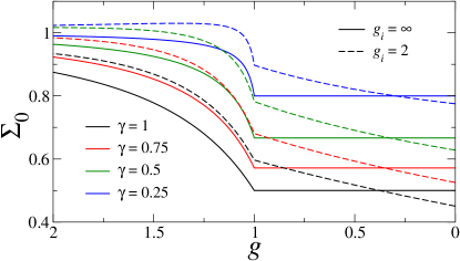
Figure 16: The large-time limit of the transverse magnetization for the quantum XY chain with different anisotropies $\gamma$ in the thermodynamic limit, as a function of $g$ and for two values of $g_{i}=\infty$ (continuous lines) or $g_{i}=2$ (dashed lines). The curves for $\Sigma_{0}$ display a singular behavior (i.e., a discontinuity in the derivative) at $g=g_{c}=1$. Adapted from Ref. [576].

Singular behaviors are also found for quenches starting from the ordered magnetized phase ($g_{i}<1$), in particular when monitoring the longitudinal (l) magnetization

$$M_{\rm l}(t)\equiv L^{-1}\sum_{x}m_{{\rm l},x}(t)\,,\qquad m_{{\rm l},x}(t)=\big{\langle}\hat{\sigma}^{(1)}_{x}\big{\rangle}_{t}\,.$$ (205)

For example, one may consider quenches of the quantum Ising chain ($\gamma=1$) starting from a completely ordered state (i.e., a fully magnetized state $|\Psi(0)\rangle=|\!\!\uparrow,\ldots,\uparrow\rangle$). This corresponds to one of the degenerate ground states in the thermodynamic limit when $g_{i}\to 0$, obtainable by the ground state $|\Psi_{0}(g_{i},h)\rangle$ in the limit

$$|\Psi(0)\rangle=\lim_{g_{i}\to 0}\lim_{h\to 0^{+}}\lim_{L\to\infty}|\Psi_{0}(g_{i},h)\rangle\,,$$ (206)

where $h$ is an external homogeneous magnetic field coupled to the longitudinal magnetization. Since such initial state breaks the $\mathbb{Z}_{2}$ symmetry of the model, one finds a nonzero longitudinal magnetization $M_{\rm l}$ along the quantum unitary evolution after quenching the transverse-field parameter $g$. In the thermodynamic limit, it vanishes in the large-time limit, showing an asymptotic exponential decay [562]

$$M_{\rm l}(t;g)\approx{\cal M}_{{\rm l},a}(t,g)={\rm A}(g)\,\exp[-\Gamma(g)\,t]\,.$$ (207)

Similarly to the transverse magnetization, there is a singular behavior at $g=g_{c}$. Indeed, around $g_{c}=1$, the decay function $\Gamma(g)$ behaves as [562, 576]

$$\Gamma(g)=\left\{\begin{array}[]{ll}4/\pi-2\sqrt{2(1-g)}+O(1-g)&{\rm for}\;g<1\,,\vspace*{2mm}\\ 4/\pi&{\rm for}\;g\geq 1\,.\end{array}\right.$$ (208)

8.7.2 Revival phenomena in finite-size systems

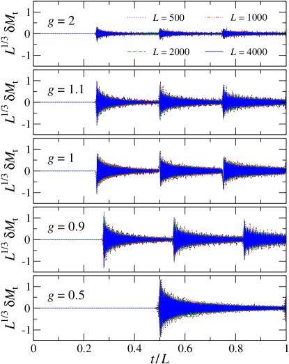
Figure 17: Finite-size features of the temporal behavior of the transverse magnetization after a quench from $g_{i}=\infty$. The figure shows $L^{1/3}\,\delta M_{\rm t}$ versus the rescaled time $t_{L}\equiv t/L$, where $\delta M_{\rm t}$ in Eq. (209) quantifies the finite-size effects. Panels from top to bottom are for $g=2,\,1.1,\,1,\,0.9,\,0.5$. Colored curves stand for various system sizes, as indicated in the legend. They support a power-law suppression of the finite-size revival effects as $L^{-1/3}$. Adapted from Ref. [576].

In finite systems, quantum quenches from the disordered phase ($g_{i}>1$) show the emergence of peculiar revival phenomena (see, e.g., Refs. [686, 687, 688, 689, 587, 690, 691, 576]). This is evident from the data shown in Fig. 17, for the subtracted transverse magnetization

$$\delta M_{\rm t}(t;L,g_{i},g)\equiv M_{\rm t}(t;L,g_{i},g)-\Sigma(t;g_{i},g)\,,$$ (209)

$\Sigma(t;g_{i},g)$ being the infinite-size limit in Eq. (202), for finite systems of size $L$ with PBC and $g_{i}\to\infty$. The numerical results show the following behavior

$$\delta M_{\rm t}(t;L)=L^{-a}f_{e}(t_{L})\,f_{o}(t;L)+O(L^{-1})\,,\qquad t_{L}\equiv t/L\,,\qquad a\approx 1/3\,,$$ (210)

where $f_{o}(t;L)$ is a rapidly oscillating function around zero depending on both $t$ and $L$, while the envelope function $f_{e}(t_{L})$ is a (non-oscillating) function of $t_{L}$ with apparent discontinuities located at $t_{L}=t_{L,k}$. This behavior of the function $f_{e}$ is essentially related to revival phenomena, which appear at times

$$t_{L,k}\equiv{k\over 2v_{m}}\,,\qquad k=1,2,\ldots\,,\qquad v_{m}=2\,{\rm Min}[g,1]\,,$$ (211)

where $v_{m}$ is the maximum velocity of the quasi-particle modes [692, 674, 562]. The amplitude of such discontinuities generally tends to decrease with increasing $k$, as it can be seen from the various panels of Fig. 17. In particular, numerical results for $g=g_{c}=1$ show that the first sharp dip is asymptotically located at $t_{L,1}=1/4+O(L^{-2/3})$. This can be related to the interference between the signals traveling in the opposite direction with velocity $v_{m}=2$, [687] taking a time $t=L/(2v_{m})=L/4$ to approach each other. The scaling behavior (210) has been observed in numerical simulations for any value of $g$; the functions $f_{e}$ and $f_{o}$ change with $g$, but maintain a similar structure. Therefore, the main features of the scaling laws associated with the finite-size revival effects (in particular its power law $L^{-1/3}$) are not related to the existence of quantum criticality at $g_{c}$.

We finally mention that similar revival phenomena are also observed when quenching from the ordered phase and looking at the longitudinal magnetization in finite-size systems [576].

8.7.3 Moving away from integrability

Numerical studies of the effects of moving Ising-like systems away from integrability, for example by adding nonintegrable Hamiltonian terms as those of the anisotropic next-to-nearest-neighbor Ising (ANNNI) models [37], have shown that some qualitative features of the post-quench dynamics persist. In particular, the evolution of the longitudinal magnetization displays qualitative differences when the quenches are performed within the ordered phase or crossing the transition point toward the disordered phase [576].

As originally proposed in Ref. [681], hard-quench protocols may be used to find evidence of phase transitions even in nonintegrable systems. For this purpose, one can exploit some features of the intermediate-time dynamics of local observables and the entanglement entropy after quantum quenches to the critical point of an underlying equilibrium QT. Numerical investigations on the derivatives of such quantities with respect to the quench parameter, in ANNNI chains, develop strong dips/peaks in the vicinity of the QT.

9 Out-of-equilibrium dynamics arising from slow Kibble-Zurek protocols

In this section we focus on the dynamics arising from slow changes of the Hamiltonian parameters across CQTs. Dynamic KZ protocols involving such slow changes are generally performed within systems described by the general Hamiltonian

$$\hat{H}(t)=\hat{H}_{c}+w(t)\,\hat{H}_{p}\,,$$ (212)

where $\hat{H}_{c}$ and $\hat{H}_{p}$ do not depend on time. As assumed in Eq. (172), also in this case we suppose that $[\hat{H}_{c},\hat{H}_{p}]\neq 0$ and that $\hat{H}_{c}$ represents a critical Hamiltonian at its CQT point. The tunable parameter $w$ controls the strength of the coupling with the perturbation $\hat{H}_{p}$, and is again taken as a relevant parameter driving the CQT, such as the longitudinal ($h$) or the transverse ($r=g-g_{c}$) external field strength in the quantum Ising models (6), or the chemical potential $r=\mu-\mu_{c}$ in the Kitaev fermionic models (8). Therefore $w_{c}=0$ corresponds to the transition point.

Across a QT, the growth of an out-of-equilibrium dynamics is inevitable in the thermodynamic limit, even for very slow changes of the parameter $w$, because large-scale modes are unable to equilibrate as the system changes phase. Indeed, when starting from the ground state associated with the initial value $w_{i}$, the system cannot pass through ground states associated with the time dependence of $w(t)$ across the transition point, thus departing from an adiabatic dynamics. This gives rise to a residual abundance of defects after crossing the transition point [693, 694, 695, 696, 539, 538, 540, 697, 4, 37, 543, 698, 5, 699, 700, 701].

9.1 Kibble-Zurek protocols

Slow (quasi-adiabatic) passages through QTs allow us to probe some universal features of quantum fluctuations in such circumstances. In this respect, a special role is played by the KZ problem [693, 695], related to the amount of final defects that are generated when slowly moving the system from the disordered to the ordered phase. KZ-like protocols have been largely employed to investigate the critical dynamics of closed systems, subject to unitary time evolutions. To this purpose, one can assume that negative values $w<0$ correspond to a gapped quantum disordered phase. Quasi-adiabatic passages through the QT are obtained by slowly varying $w$ across $w_{c}=0$, following, e.g., the standard procedure:

• One starts from the ground state of the many-body system at $w_{i}<0$, given by $|\Psi(t=0)\rangle\equiv|\Psi_{0}(w_{i})\rangle$.

• Then the out-equilibrium unitary dynamics, ruled by the Schrödinger equation

  $${{\rm d}\,|\Psi(t)\rangle\over{\rm d}t}=-i\,\hat{H}(t)\,|\Psi(t)\rangle\,,$$ (213)

  arises from a linear dependence of the time-dependent parameter $w(t)$, such as

  $$w(t)=c\,t\,,\qquad t_{s}\equiv c^{-1}>0\,,$$ (214)

  up to a final value $w_{f}>0$. Therefore the KZ protocol starts at time $t_{i}=t_{s}\,w_{i}<0$ and stops at $t_{f}=t_{s}\,w_{f}>0$. The parameter $t_{s}$ denotes the time scale of the slow variations of the Hamiltonian parameter $w$ .

The resulting out-of-equilibrium evolution of the system can be investigated by monitoring observables and correlations at fixed time, such as those reported in Sec. 8.1. Other similar protocols have been introduced (see, e.g., Refs. [4, 543]), for example crossing the QT with different power-law dependencies of $w(t)$. The scaling laws reported below can be straightforwardly adapted to these more general cases.

9.2 The Kibble-Zurek mechanism

The so-called KZ mechanism, associated with slow passages through critical points, was introduced by Kibble [693, 694] in the context of the expanding universe arising from the Big Bang, and then recast in the language of critical phenomena by Zurek [695]. Their proposal is a theory of the defects generated in a system being slowly cooled across a continuous phase transition. The system inevitably goes out of equilibrium, ending up in the broken-symmetry phase with different spatial regions realizing different orientations of the broken symmetry, and topological defects as a result.

The KZ problem [696] at CQTs is related to the abundance of defects arising from the KZ protocol due to the inevitable loss of adiabaticity when crossing a CQT, even in the limit of very slow variations of the driven parameter. For asymptotically slow changes of the parameters around the CQT, the dynamic behavior is expected to be essentially controlled by the universal features associated with the universality class of the equilibrium CQT. Far away from the critical point within the disordered phase [i.e., $w(t)\lesssim-1$], the equilibrium relaxation time $t_{r}$ is very small with respect to the time scale $t_{s}$ of the variation of $w$, thus enabling an adiabatic dynamics through the ground states at the instantaneous values of $w(t)$. On the other hand, close to the transition point [i.e., $|w(t)|\ll 1$], the dynamics gets approximately frozen, due to the divergence of the equilibrium relaxation time (critical slowing down), behaving as $t_{r}\sim|w|^{-z\nu}$. The critical modes cannot adjust to the change of the driving parameter $w(t)$, giving rise to an out-of-equilibrium dynamics.

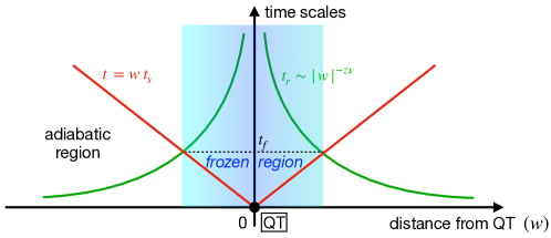
Figure 18: A sketch containing the idea beyond the KZ mechanism. The green and red curves respectively indicate the relaxation time $t_{r}$ and the time $t$ to reach the QT point (located at $w=0$), as a function of the parameter $w$. The intersection between the two curves denotes the time $t_{f}$ at which the system ceases to behave adiabatically and enters a region where the dynamics remains approximately frozen.

A phenomenological derivation of the KZ mechanism has been reported in the pioneering works [693, 695, 539] and is sketched in Fig. 18. The turning point from the adiabatic to the out-of-equilibrium frozen regime occurs at the time $t_{f}$ when the relaxation time $t_{r}$ is of the order of the remaining time to reach the value $w=0$,

$$t_{r}\sim|w(t_{f})|^{-z\nu}\approx|t_{f}|\,,\quad{\rm thus}\quad|t_{f}|\sim t_{s}^{z\nu/(1+z\nu)}\,.$$ (215)

Such freezing time $t_{f}$ allows us to define a corresponding length scale $\lambda_{f}\equiv(t_{f}/t_{s})^{-\nu}=t_{s}^{\nu/(1+z\nu)}$. The number of defects eventually emerging from the frozen region is thus expected to follow the power law

$$\rho_{\rm def}\sim\lambda_{f}^{-d}=t_{s}^{-{d\nu\over 1+z\nu}}\,.$$ (216)

An analogous power law can be also derived by arguments based on the adiabatic perturbation theory [538, 4, 37, 5].

We mention that, beside the average density of defects $\rho_{\rm def}$, also the corresponding full counting statistics can be shown to exhibit universal features. In particular, all the cumulants of the defects number distribution (including the variance, third-centered moment, etc.) inherit a universal power-law scaling with the driving time, thus generalizing the KZ prediction of Eq. (216) [702, 703].

9.3 Dynamic scaling arising from Kibble-Zurek protocols

Dynamic scaling laws are expected to develop in the limit of large time scale $t_{s}$ of the driven parameter $w(t)$. A phenomenological scaling theory is obtained by assuming the homogeneous scaling laws reported in Sec. 8.2, taking into account that the parameter $w(t)=t/t_{s}$ has a linear time dependence, when crossing the critical point $w=0$. For example, for generic observables and correlation functions defined using local operators $\hat{O}$, we consider the homogeneous scaling laws

$$O(t,t_{s};L,w_{i})\!\! \!\!\equiv\!\! \!\!\big{\langle}\hat{O}\big{\rangle}_{t}\approx b^{-y_{o}}\,{\cal O}(b^{-z}t,b^{y_{w}}w(t),b^{-1}L,b^{y_{w}}w_{i})\,,$$ (217a)

$$G_{12}(t,t_{s},{\bm{x}};L,w_{i})\!\! \!\!\equiv\!\! \!\!\big{\langle}\hat{O}_{1}({\bm{x}}_{1})\hat{O}_{2}({\bm{x}}_{2})\big{\rangle}_{t}\approx b^{-\varphi_{12}}\,{\cal G}_{12}(b^{-z}t,b^{y_{w}}w(t),b^{-1}{\bm{x}},b^{-1}L,b^{y_{w}}w_{i})\,,\qquad$$ (217b)

as working hypotheses for the derivation of the dynamic scaling laws in the thermodynamic and FSS limits .

9.3.1 Dynamic scaling in the thermodynamic limit

To derive a dynamic scaling theory for infinite-volume systems, it is possible to exploit the arbitrariness of the scale parameter $b$ in Eqs. (46). For this purpose we set

$$b=\lambda\equiv t_{s}^{1\over y_{w}+z}\,,$$ (218)

where $\lambda$ is the length scale associated with the KZ protocol, and take the thermodynamic limit $L/\lambda\to\infty$. By simple manipulations, this leads to the dynamic KZ scaling ansatze

$$O(t,t_{s};w_{i})\approx\lambda^{-y_{o}}\,{\cal O}_{\infty}(\Omega_{t},\lambda^{y_{w}}w_{i})\,,\qquad G_{12}(t,t_{s},{\bm{x}};w_{i})\approx\lambda^{-\varphi_{12}}\,{\cal G}_{\infty}(\Omega_{t},{\bm{x}}/\lambda,\lambda^{y_{w}}w_{i})\,,$$ (219)

where $\Omega_{t}$ is the rescaled time

$$\Omega_{t}\equiv{t\over t_{s}^{\kappa}}\,,\qquad\kappa={z\over y_{w}+z}\,.$$ (220)

The dynamic KZ scaling limit, where the above asymptotic behaviors apply, is obtained by taking $t_{s}\to\infty$, keeping the arguments of the scaling functions ${\cal O}_{\infty}$ and ${\cal G}_{\infty}$ fixed. Actually, introducing a temporal scaling variable related to the initial time of the KZ protocol, defined as

$$\Omega_{t_{i}}\equiv{t_{i}\over t_{s}^{\kappa}}\,,\qquad t_{i}=w_{i}\,t_{s}\,,$$ (221)

we may rewrite the scaling Eqs. (219) as

$$O(t,t_{s};w_{i})\approx\lambda^{-y_{o}}\,\widetilde{\cal O}_{\infty}(\Omega_{t},\Omega_{t_{i}})\,,\qquad G_{12}(t,t_{s},{\bm{x}};w_{i})\approx\lambda^{-\varphi_{12}}\,\widetilde{\cal G}_{\infty}(\Omega_{t},{\bm{x}}/\lambda,\Omega_{t_{i}})\,.$$ (222)

Since the KZ protocol starts from $w_{i}<0$ corresponding to the gapped phase, whose gap decreases as $\Delta\sim\xi^{-z}$ and the ground-state length scale $\xi$ diverges only at the critical point $w=0$, the emerging dynamic KZ scaling should be independent of the actual finite value of $w_{i}<0$, if this is kept fixed in the KZ scaling limit. This is due to the fact that, in a gapped phase, the evolution arising from slow changes of the parameters is essentially adiabatic, from $w_{i}$ to the relevant scaling interval $I_{w}$ around $w=0$, which effectively decreases as

$$I_{w}\sim t_{s}^{-1+\kappa}\;\to\;0$$ (223)

in the dynamic KZ scaling limit. Therefore, when increasing $t_{s}$, keeping $w_{i}<0$ constant and finite, the dynamic KZ scaling must be independent of $w_{i}$, corresponding to the $\Omega_{t_{i}}\to-\infty$ limit of the relations (222). When keeping $w_{i}<0$ fixed, this leads to the dynamic scaling ansatze

$$O(t,t_{s};w_{i})\approx\lambda^{-y_{o}}\,{\cal O}_{\infty}(\Omega_{t})\,,\qquad G_{12}(t,t_{s},{\bm{x}};w_{i})\approx\lambda^{-\varphi_{12}}\,{\cal G}_{\infty}(\Omega_{t},{\bm{x}}/\lambda)\,,$$ (224)

for fixed-time observables. These scaling laws can be extended to correlations at different times [543].

One may also define an out-of-equilibrium correlation length $\xi_{\rm KZ}(t)$ from the large-distance exponential decay of the two-point equal-time correlation function of the site variables, or its second moment. Using the above scaling behaviors, in particular Eq. (224), one gets this scaling ansatz (keeping $w_{i}$ fixed):

$$\xi_{\rm KZ}(t,t_{s})\approx t_{s}^{\kappa/z}\,{\cal L}(\Omega_{t})\,.$$ (225)

The dynamic scaling functions introduced above are expected to be universal with respect to changes of the microscopic details of the Hamiltonian within the given universality class. Of course, like any scaling function at QTs, such a universality holds, apart from a multiplicative overall constant and normalizations of the scaling variables. The approach to the asymptotic dynamic scaling behavior is expected to be generally characterized by power-law suppressed corrections, such as those discussed at equilibrium (see Sec. 4).

As already mentioned, the so-called KZ problem genuinely addresses the formation of defects when slowly crossing the QT, from the disordered to the ordered phase. The defect number arising from the out-of-equilibrium condition is expected to scale as the inverse of the scaling volume, that is,

$$\rho_{\rm def}\sim\xi_{\rm KZ}^{-d}\approx t_{s}^{-{d\over y_{w}+z}}\,{\cal R}_{\rm def}(\Omega_{t})\,,$$ (226)

in agreement with Eq. (216) identifying $y_{w}=1/\nu$. However, we should note that Eq. (226) is derived in the KZ scaling limit, i.e., in the large-$t_{s}$ limit keeping $\Omega_{t}=t/t_{s}^{\kappa}$ finite, or equivalently when the final value $w_{f}$ of $w$ scales appropriately around $w=0$ (i.e., as $w_{f}\sim t_{s}^{-1+\kappa}$ when increasing $t_{s}$). In the large-$\Omega_{t}$ limit, important dynamic effects related to the ordered region and its degenerate lowest states may set in, particularly when the global symmetry is preserved by the KZ protocol and its initial state. Therefore, the determination of the asymptotic power law of the defect number would also require some knowledge of the asymptotic behavior of the scaling function ${\cal R}_{\rm def}(\Omega_{t})$ in Eq. (226). In particular, in order to recover the KZ prediction (216) from the scaling law (226), it is required that $\lim_{\Omega_{t}\to\infty}{\cal R}_{\rm def}(\Omega_{t})$ converges to a finite and constant value. This issue is relevant for possible comparisons of the KZ prediction (216) for the number of defects with measurements taken in the very large time limit, deep in the ordered phase.

For example, classical systems show coarsening phenomena when they are quenched to an ordered phase with multiple degenerate low-energy states. Local broken-symmetry regions grow in time and the system is asymptotically self-similar on a characteristic coarsening length scale $\ell_{c}$, which generally increases as a power law of the time [529]. The correlation functions approach their equilibrium value on the scale $\xi_{e}\ll\ell_{c}$ within each quasi-homogeneous domain, but they get exponentially suppressed between different domains. In the late-time regime, a dynamical coarsening scaling is eventually realized when there are no growing scales competing with $\ell_{c}$. As argued in Ref. [543], coarsening dynamic phenomena are expected to become relevant in the large-time regime of the KZ protocols, deep in the ordered phases, determining the asymptotic $\Omega_{t}\to\infty$ behavior of the KZ scaling functions.

The general features of the KZ dynamic scaling in the thermodynamic limit, and in particular the KZ predictions for the abundance of residual defects, have been confirmed by several analytical and numerical studies (see, e.g., Refs. [4, 37, 5, 543, 704] and citing references). In particular, the computations [540, 705, 4] for Ising and XY chains using KZ protocols driven by the transverse field $g$ confirm the scaling behavior predicted by Eq. (226), i.e. $\rho_{\rm def}\sim t_{s}^{-1/2}$. Further results supporting the KZ dynamic scaling will be presented in Sec. 9.4 for the related fermionic Kitaev wire. The KZ defect production has been also investigated at multicritical points [706, 707, 708]. Results for quantum-information quantities, such as the entanglement, the concurrence and the discord, during KZ protocols can be found in Refs. [709, 710, 711, 704, 712, 713, 714]. We finally mention that the scaling law of the abundance of residual defects after crossing phase transitions has been also verified in experiments for various physically interesting systems (see, e.g., Refs. [715, 716, 554, 533, 717, 718, 534, 535, 536, 579, 189, 188, 719, 720, 721, 722, 723].

9.3.2 Dynamic finite-size scaling

The scaling Eqs. (46) allow to derive dynamic FSS relations, which are valid far from the thermodynamic limit, and which extend those predicted by the FSS theory for systems at equilibrium. For example, by setting $b=L$ in Eq. (178b), we obtain

$$G_{12}(t,t_{s},{\bm{x}};L,w_{i})\approx L^{-\varphi_{12}}\,{\cal G}_{L}(\Theta,{\bm{X}},L^{y_{w}}t/t_{s},\Omega_{t_{i}})\,,$$ (227)

where ${\bm{X}}={\bm{x}}/L$, $\Theta=L^{-z}t$, $\Omega_{t_{i}}=L^{y_{w}}w_{i}$, similarly to the case of quantum quench protocols, cf. Eq. (182).

This dynamic FSS behavior is expected to be obtained by taking $L\to\infty$, while keeping the arguments of the scaling function ${\cal G}_{L}$ fixed. One may introduce more convenient scaling variables, which are combinations of those entering Eq. (227). For example, one can write it as

$$G_{12}(t,t_{s},{\bm{x}};L,w_{i})\approx L^{-\varphi_{12}}\,\widetilde{\cal G}_{L}(\Omega_{t},{\bm{X}},\Upsilon,\Omega_{t_{i}})\,,$$ (228)

where

$$\Upsilon\equiv{t_{s}\over L^{y_{w}+z}}\,,$$ (229)

and $\Omega_{t},\,\Omega_{t_{i}}$ are defined in Eqs. (220) and (221), respectively.

Assuming again that the KZ protocol starts from the gapped disordered phase and that the initial $w_{i}<0$ is kept fixed in the dynamic scaling limit, the same dynamic FSS is expected to hold, irrespective of the value of $w_{i}$. Thus, the dynamic FSS behavior in Eq. (228) simplifies into

$$G_{12}(t,t_{s},{\bm{x}};L,w_{i})\approx L^{-\varphi_{12}}\,{\cal G}_{L,\infty}(\Omega_{t},{\bm{X}},\Upsilon)\,.$$ (230)

Indeed, with increasing $L$, the dynamic FSS occurs within a smaller and smaller interval $I_{w}$ of values of $|w|$ around $w=0$: since the time interval of the out-of-equilibrium process described by the scaling laws scales as $t_{\rm KZ}\sim t_{s}^{\kappa}$, the relevant interval $I_{w}$ of values of $|w|$ shrinks as

$$I_{w}\sim{t_{\rm KZ}/t_{s}}\sim L^{-y_{w}}\,,$$ (231)

when keeping $\Upsilon$ fixed.

Note that, in the limit $\Upsilon\to\infty$, the evolution as a function of $w(t)=t/t_{s}$ corresponds to an adiabatic dynamics. Indeed, since the finite size $L$ guarantees the presence of a gap between the lowest states, one may adiabatically cross the critical point if $\Upsilon\to\infty$, passing through the ground states of the finite-size system for $w(t)$. The adiabatic evolution across the transition point is prevented only when $L\to\infty$ (before the limit $t_{s}\to\infty$), i.e., when the time scale $t_{r}$ of the critical correlations diverges, as $t_{r}\sim\Delta^{-1}\sim L^{z}$.

9.4 Kibble-Zurek protocols within the 1$d$ Kitaev model

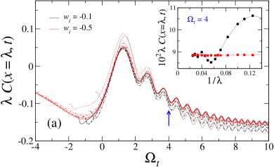
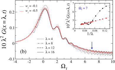
Figure 19: Rescaled correlations $\lambda\,C(x,t)$ $(a)$ and $\lambda^{2}\,G(x,t)$ $(b)$, at fixed $x/\lambda=1$ (results for other values of $x/\lambda$ show analogous behaviors), for the unitary dynamics of the Kitaev quantum wire in the thermodynamic limit, as a function of the rescaled time $\Omega_{t}$. The correlation functions $C$ and $G$ are defined in Eqs. (232b) and (232c), respectively. Different line styles stand for various values of the length scale $\lambda$, from $4$ to $16$ [see legend in ($b$)]. Data belonging to one of the two color sets correspond to a given initial Hamiltonian parameter $w_{i}<0$, which is kept fixed and equal to either $w_{i}=-0.1$ (black curves and circles) or $w_{i}=-0.5$ (red curves and squares). The insets in the two panels display rescaled correlations as a function of $1/\lambda$, for both cases of $w_{i}$ presented in the main frames, at the $\Omega_{t}$ value indicated by the blue arrow. In the figure, time evolutions up to length scales $\lambda\sim 50$ are shown [corresponding to time scales $t_{s}=\lambda^{y_{w}+z}=\lambda^{2}$ of the order $O(10^{3})$], and have been obtained from much larger systems of size $L=4096$. Analogous results are obtained for the correlation function $P$, cf. Eq. (232a). Adapted from Ref. [650].

The KZ scaling behaviors in the thermodynamic and FSS limits can be accurately checked within the paradigmatic 1$d$ Kitaev fermionic chain (8), for which results for very large systems can be obtained by diagonalizing the Hamiltonian, as outlined in Sec. 3.1. We remark that, although the XY chain (7) can be exactly mapped into the Kitaev quantum wire in the thermodynamic limit, differences emerge when finite-size systems are considered, because the nonlocal Jordan-Wigner transformation does not preserve the BC (see the discussion in Sec. 3.1.3), with the exception of the simplest OBC. In particular, Kitaev quantum wires with PBC or ABC do not map into XY chains with analogous BC. This point is particularly relevant for the dynamic FSS. For example, as already mentioned, the Hilbert space of the Kitaev quantum wire with ABC is restricted with respect to that of the quantum Ising chain, so that it is not possible to restore the competition between the two vacua belonging to the symmetric/antisymmetric sectors of the XY chain [106, 107, 86], controlled by the symmetry-breaking longitudinal field $h$.

The Kitaev quantum wire in Eq. (8) undergoes a CQT at $\mu_{c}=-2$, independently of $\gamma$, belonging to the 2$d$ Ising universality class. Thus we introduce the relevant parameter $w=\mu-\mu_{c}$, whose RG dimension $y_{w}=1$ determines the length-scale critical exponent $\nu=1/y_{w}=1$. The dynamic exponent associated with the unitary quantum dynamics is $z=1$. To characterize the quantum evolution, various fixed-time correlations of fermionic operators can be considered, such as

$$P(x,t)\!\! \!\!\equiv\!\! \!\!\big{\langle}\hat{c}_{j}^{\dagger}\hat{c}_{j+x}^{\dagger}+\hat{c}_{j+x}\hat{c}_{j}\big{\rangle}_{t}\,,$$ (232a)

$$C(x,t)\!\! \!\!\equiv\!\! \!\!\big{\langle}\hat{c}_{j}^{\dagger}\hat{c}_{j+x}+\hat{c}_{j+x}^{\dagger}\hat{c}_{j}\big{\rangle}_{t}\,,$$ (232b)

$$G(x,t)\!\! \!\!\equiv\!\! \!\!\big{\langle}\hat{n}_{j}\hat{n}_{j+x}\big{\rangle}_{t}-\big{\langle}\hat{n}_{j}\big{\rangle}_{t}\,\big{\langle}\hat{n}_{j+x}\big{\rangle}_{t}\,,$$ (232c)

where $$j,x\in[1,L/2] t w_{i}=\mu_{i}-\mu_{c}$$, and averages are calculated over the state of the system at time , arising from the KZ protocol described in Sec. 9.1, and starting from the ground state associated with .

According to the scaling arguments outlined in Sec. 9.4, these correlation functions are predicted to show dynamic scaling behaviors. In particular, Eqs. (224) and (230) are expected to describe their asymptotic dynamic KZ scaling in the thermodynamic and FSS limits, respectively, when the initial parameter $w_{i}$ is kept fixed in the dynamic KZ limit, so that its dependence asymptotically disappears. The corresponding exponents are $\varphi_{12}=1$ for the correlations $P$ and $C$, and $\varphi_{12}=2$ for $G$, according to the RG dimensions $y_{c}=1/2$ of the fermionic operators $\hat{c}_{x}$, and $y_{n}=1$ of the density operator $\hat{n}_{x}$ [1].

Numerical results for the Kitaev wire with ABC (which are particularly convenient for computations) confirm the dynamic KZ scaling predictions for the above correlation functions. In particular, Fig. 19 reports some results for the correlations $C(x,t)$ and $G(x,t)$ in the thermodynamic limit, keeping the initial parameter $w_{i}$ fixed (two values of $w_{i}$ are considered in the figure). The results also show that the asymptotic scaling behaviors match for different starting point $w_{i}$, thus confirming that the asymptotic dynamic scaling is independent of $w_{i}$, when this is kept fixed. Fig. 20 shows some results for the same correlation functions in the FSS limit. Again the predicted asymptotic scaling behavior is clearly approached, with scaling corrections that are typically $O(1/L)$.

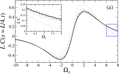
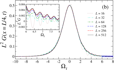
Figure 20: Rescaled correlations $L\,C(x,t)$ $(a)$ and $L^{2}\,G(x,t)$ $(b)$, defined in Eqs. (232b) and (232c) respectively, as a function of the rescaled time $\Omega_{t}$, fixing the initial Hamiltonian parameter $w_{i}=-0.5$. We also fix $x/L=1/4$ and $\Upsilon=0.1$. Different lines are for various sizes $L$, as indicated in the legend. The insets show magnifications of the main frames in the regions $6\leq\Omega_{t}\leq 8$ enclosed in the blue boxes, to highlight discrepancies that reduce with increasing $L$. Analogous results can be obtained for the correlation function $P$, cf. Eq. (232a).

9.5 Quantum annealing

We finally discuss a somehow related issue, which deals with the quantum dynamics arising from a gentle modulation in time of one of the Hamiltonian control parameters. The principle of adiabatic quantum dynamics has been adopted in recently developed quantum devices for quantum-computation purposes (see, e.g., Refs. [724, 725] and citing references). This leads to the so-called adiabatic quantum computing, whose key principle is very simple: evolving a quantum system from the ground state of a given Hamiltonian $\hat{H}_{i}$ to that of another Hamiltonian $\hat{H}_{f}$, which encodes the solution to the problem of interest. The evolution should be performed in such a way that the system is always in its instantaneous ground state, by slowly varying the parameter $s(t):0\to 1$ in the Hamiltonian

$$\hat{H}[s(t)]=\big{[}1-s(t)\big{]}\,\hat{H}_{i}+s(t)\,\hat{H}_{f}\,,\qquad s(t_{i})=0\,,\quad s(t_{f})=1\,,$$ (233)

and such protocol is usually referred to as quantum annealing [726, 727, 728].

Among the possible quantum annealing protocols, a particularly relevant case is found when crossing a QT, an occurrence giving rise to the KZ mechanism, which also emerges when hard problems are addressed. This kind of situation has been already implemented on physical systems made of superconducting qubits [729] and of trapped ions [730], with the purpose to measure the mean number of topological defects (and the cumulants of the distribution) generated by the (quasi-)adiabatic passage across the QCP of prototypical many-body models, as the quantum Ising chain in a transverse field. However, it was soon realized that dissipation in certain physical devices might play an important role (see also Sec. 14).

For practical purposes, it can be shown that the solution to computationally “hard” (NP) problems, encoded into the ground state of $\hat{H}_{f}=\hat{H}[s(t_{f})]$, cannot be adiabatically connected with the ground state of an “easy” Hamiltonian $\hat{H}_{i}=\hat{H}[s(t_{i})]$. Indeed such connection typically reflects into the passage through a FOQT, where the gap may close exponentially with the system size, thus requiring an exponentially large amount of time for the annealing process to reach the target state [731, 732, 733].

10 Dynamic finite-size scaling at first-order quantum transitions

In this section we focus on systems at FOQTs, showing that they develop a dynamic FSS besides the equilibrium FSS outlined in Sec. 5. In particular, even the dynamic behavior across a FOQT is dramatically sensitive to the BC, giving rise to out-of-equilibrium evolutions with exponential or power-law time scales, unlike CQTs where the power-law time scaling is generally independent of the type of boundaries. Again, this is essentially related to the sensitivity of the energy difference of the lowest states to the boundaries, whether they are neutral or favor one of the two phases separated by the FOQT. In particular, exponentially large time scales are expected when the boundaries are such to give rise to a quasi-level-crossing scenario, with exponentially suppressed energy differences of the two lowest levels with respect to the rest of the spectrum at larger energy, while power-law time scales are expected for boundaries favoring domain walls, for which the low-energy spectrum is dominated by their dynamics.

In the following, we consider again dynamic protocols entailing instantaneous or slow changes of the Hamiltonian parameter, as outlined in Secs. 8.1 and 9.1, respectively. Specifically, the Hamiltonian is supposed to be written as in Eq. (212), being the sum of two terms, $\hat{H}(t)=\hat{H}_{c}+w(t)\hat{H}_{p}$, where the unperturbed term $\hat{H}_{c}$ assumes the parameter values corresponding to a FOQT, and the other one $\hat{H}_{p}$ may be associated with an external varying magnetic field. For the quantum Ising models (6), $\hat{H}_{c}$ may correspond to $h=0$ and any point along the FOQT line for $g<g_{c}$. Therefore, $w$ corresponds to the magnetic field $h$.

As we shall see, the equilibrium FSS theory at FOQTs outlined in Sec. 5 can be straightforwardly extended, essentially by allowing for a time dependence associated with the further scaling variable

$$\Theta\equiv\Delta(L)\>t\,,$$ (234)

besides those already introduced at equilibrium, analogously to the case of the dynamic FSS at CQTs [see Eq. (177) in Sec. 8.2]. Again, note that the size dependence of the time scaling variable $\Theta$ may be exponential or power law, depending on the boundaries and the corresponding size dependence of the gap $\Delta(L)$. For the sake of concreteness, we will focus on the 1$d$ Ising chain, thus along its FOQT line for $g<g_{c}=1$. However, analogous behaviors are expected for larger dimensions, with the appropriate correspondence of the BC.

We mention that FOQTs have been studied in the context of adiabatic quantum computation as well (see, e.g., Refs. [734, 735, 150]), due to their peculiar features of realizing an exponentially suppressed energy difference of the lowest eigenstates. Moreover, the out-of-equilibrium dynamical behavior has been also investigated at classical first-order transitions, driven by the temperature or by external magnetic fields (see, e.g., Refs. [113, 736, 737, 544, 738, 739, 740, 741]).

10.1 Quantum quenches at first-order quantum transitions

As described in Sec. 8.1, the quench protocol introduces the parameter $w_{i}$ determining the initial ground state, and then the parameter $w\neq w_{i}$ determining the quantum evolution, according to Eq. (173). The dynamic FSS of observables can be obtained by extending the one at equilibrium, cf. Eq. (99), allowing for a time dependence through the scaling variable $\Theta$ defined in Eq. (234). We also need the scaling variables $\Phi_{i}$ and $\Phi$ associated with the values of $w_{i}$ and $w$ involved in the quench protocol, which can be defined as in Eq. (95), replacing $h$ with $w_{i}$ and $w$, respectively. The dynamic FSS limit is defined as the infinite-size limit, keeping the scaling variables $\Phi_{i}$, $\Phi$ and $\Theta$ fixed. In this limit, the central-lattice and global magnetizations are expected to behave as

$$M(t;L,w_{i},w)\approx m_{0}\,{\cal M}(\Theta,\Phi_{i},\Phi)\,,$$ (235)

where $m_{0}$ is the infinite-size magnetization approaching the FOQT in the limit $h\to 0^{+}$, cf. Eq. (15). This scaling behavior is expected to hold for any $g<1$, and the scaling function ${\cal M}$ should be independent of $g$, apart from trivial normalizations of the arguments. However, analogously to equilibrium FSS at FOQTs, the size-dependence of the scaling variables and the form of ${\cal M}$ significantly depend on the BC.

The above dynamic scaling relations can be straightforwardly extended to any FOQT, by identifying the scaling variable $\Phi$ as the ratio $\delta E_{p}(L)/\Delta(L)$, where $\delta E_{p}(L)$ is the energy variation associated with the perturbation $w\hat{H}_{p}$ and $\Delta(L)$ is the energy difference between the two lowest states at the transition point. The scaling variable $\Theta$ associated with time is always defined as in Eq. (234).

10.1.1 Neutral boundary conditions

In the case of neutral boundary conditions, such as OBC or PBC, one may again exploit the two-level truncation to compute the scaling function ${\cal M}$ associated with the magnetization, extending the equilibrium computation reported in Sec. 5.3. As shown in Ref. [527], in the long-time limit and for large systems, the scaling properties in a small interval around $w=0$ are captured by a two-level truncation, restricting the problem to the two nearly-degenerate lowest-energy states. More precisely, this approximation is appropriate when

$$\delta E_{w}(L,w)=2m_{0}|w|L^{d}=|\Phi|\,\Delta(L)\ll E_{2}(L)-E_{0}(L)\,.$$ (236)

In the case at hand (i.e., for systems with PBC or OBC), $E_{2}(L)-E_{0}(L)=O(1)$ in the large-$L$ limit.

The effective quantum evolution with the reduced two-dimensional Hilbert space is determined by the Schrödinger equation with the truncated Hamiltonian $\hat{H}_{2}(w)$, cf. Eq. (104), using the two-component ground state corresponding to $w_{i}$ as initial condition at $t=0$. Simple calculations show that, apart from an irrelevant phase, the time-dependent state $|\Psi_{2}(t)\rangle$ evolves as [527],

$$|\Psi_{2}(t)\rangle=\cos\left({\alpha_{i}-\alpha\over 2}\right)|0\rangle+e^{-i\,\Theta\sqrt{1+\Phi^{2}}}\sin\left({\alpha_{i}-\alpha\over 2}\right)|1\rangle\,,$$ (237)

with $\tan\alpha_{i}=\Phi_{i}^{-1}$, $\tan\alpha=\Phi^{-1}$, and

$$|0\rangle=\sin(\alpha/2)\,|-\rangle+\cos(\alpha/2)\,|+\rangle\,,\qquad|1\rangle=\cos(\alpha/2)|-\rangle-\sin(\alpha/2)\,|+\rangle\,,$$ (238)

$|\pm\rangle$ being the eigenstates of the operator $\hat{\sigma}^{(3)}$. Then, the expectation value $\langle\Psi_{2}(t)|\hat{\sigma}^{(3)}|\Psi_{2}(t)\rangle$ gives the magnetization, which produces the following dynamic scaling function defined in Eq. (235):

$${\cal M}=\cos(\alpha-\alpha_{i})\cos\alpha+\cos\big{(}\Theta\sqrt{1+\Phi^{2}}\big{)}\sin(\alpha-\alpha_{i})\sin\alpha\,.$$ (239)

Numerical results for the Ising chain with PBC [527] have shown that the above scaling behavior is rapidly approached with increasing $L$ (corrections in $L$ appear exponentially suppressed), confirming that, when the energy scale of the dynamic process is of the order of the energy difference of the lowest states, the dynamics is effectively described by restricting the problem to the two lowest-energy states of the Hilbert space. The above behavior is expected at FOQTs where the two-level scenario applies, therefore it holds for generic quantum Ising models in any dimension, along their FOQT line. In a sense, the two-level model thus represents a large universality class for the asymptotic dynamic FSS at FOQTs.

An analysis of the work fluctuations in quenches at FOQT is reported in Ref. [573], where the scaling predictions are compared with computations within the two-level framework. Again, numerical results nicely support them.

We finally mention that in the case of EFBC, favoring a magnetized phase, such as those discussed in Sec. 5.5, the situation is subtler, due to the fact that the pseudo critical point is shifted. However, the two-level scenario applies as well, in the appropriate limit [649].

10.1.2 Boundary conditions giving rise to domain walls

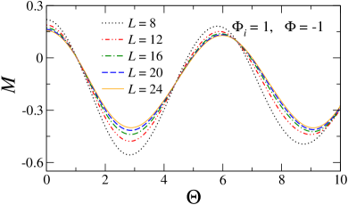
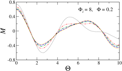
Figure 21: Average magnetization $M$ for the quantum Ising chain with OFBC, after a sudden quench of the longitudinal field close to the FOQT, as a function of the rescaled time variable $\Theta\sim L^{-2}\,t$. We fix $g=0.5$ and the values of the rescaled variables $\Phi_{i}$ and $\Phi$ (see legends in the two panels). Different data sets are for various chain lengths $L$, as indicated in the legend. In both cases, as $L$ increases, the data nicely approach an asymptotic scaling function. Adapted from Ref. [649].

The two-level scenario does not apply to BC giving rise to domain walls, such as Ising chains with ABC and OFBC, see Sec. 5.4, where the gap turns out to behave as $\Delta(L)\sim L^{-2}$. However the dynamic FSS behavior (235) holds as well, with the appropriate scaling variables [649], as shown in Fig. 21. Analogous scaling behaviors are expected in higher dimensions, for example in the presence of more involved situations as for mixed boundaries, such as ABC or OFBC along one direction, and PBC or OBC along the others.

10.2 Dynamic scaling arising from Kibble-Zurek protocols

We now focus on the dynamic behavior arising from show changes of the Hamiltonian parameter $w(t)$, such as the KZ protocol outlined in Sec. 9. In particular, we discuss the case in which the initial value $w_{i}<0$ is kept fixed in the large-$L$ limit. Since the equilibrium FSS should be recovered in the appropriate limit, one of the scaling variables can be obtained from the equilibrium scaling variable introduced in Eq. (95), by replacing $h$ with $w(t)$, i.e., we consider

$$\Phi_{\rm KZ}\equiv{2m_{0}\,w(t)\,L^{d}\over\Delta(L)}={2m_{0}tL^{d}\over\Delta(L)\>t_{s}}\,.$$ (240)

As a further scaling variable associated to the time, we may take again $\Theta=\Delta(L)\,t$. Let us also define the related useful scaling variable

$$\Upsilon\equiv{\Theta\over\Phi_{\rm KZ}}={\Delta^{2}(L)\>t_{s}\over 2m_{0}L^{d}}\,.$$ (241)

The dynamic FSS limit corresponds to $t,t_{s},L\,\to\infty$, keeping the above scaling variables fixed. In this limit the magnetization is expected to show the dynamic FSS behavior

$$M(t,t_{s};w_{i},L)\approx m_{0}\,{\cal M}(\Upsilon,\Phi_{\rm KZ})\,,$$ (242)

independently of $w_{i}<0$. In the adiabatic limit ($t,t_{s}\to\infty$ at fixed $L$ and $t/t_{s}$), ${\cal M}(\Upsilon\to\infty,\Phi_{\rm KZ})$ must reproduce the equilibrium FSS function (99). The scaling functions are expected to be universal (i.e., independent of $g$ along the FOQT line, for a given class of BC). Note that the dynamic FSS behavior develops in a narrow range of $w(t)\approx 0$; indeed, since $\Phi_{\rm KZ}$ is kept fixed in the dynamic FSS limit, the relevant scaling behavior develops within a range $I_{w}\sim\Delta/L^{d}$, thus the interval $I_{w}$ rapidly shrinks when increasing $L$. This implies that the dynamic FSS behavior is independent of the initial value ($w_{i}$) of $w$.

The above scaling behaviors are expected to hold both for neutral boundaries, such as PBC and OBC, and for BC giving rise to domain walls, by inserting the corresponding gap $\Delta(L)$. Moreover, they are quite general and can be straightforwardly extended to any FOQT, with the appropriate correspondences. Below we discuss the case of neutral boundaries, for which the scaling functions can be computed by resorting to the two-level framework. Results for other BC can be found in Ref. [649].

Within the two-level reduction of the problem, the effective time-dependent Hamiltonian reads

$$\hat{H}_{r}=\varepsilon(t)\,\hat{\sigma}^{(3)}+\zeta\,\hat{\sigma}^{(1)}\,,\qquad\varepsilon(t)={m_{0}\,w(t)\,L^{d}}=m_{0}tL^{d}/t_{s}\,,\qquad\zeta=\Delta(L)/2\,.$$ (243)

The dynamics is analogous to that governing a two-level quantum mechanical system in which the energy separation of the two levels is a function of time, which is known as the Landau-Zener problem [742, 743]. Therefore, the two-component time-dependent wave function for the quantum Ising ring can be derived from the corresponding solutions [744]. If $|\Psi_{2}(t)\rangle$ is the solution of the Schrödinger equation with the initial condition $|\Psi_{2}(t_{i})\rangle=|+\rangle$ (where $|+\rangle$ is the positive eigenvalue of $\hat{\sigma}^{(3)}$), the dynamic FSS function of the magnetization can be computed by taking the expectation value

$${\cal M}(\Upsilon,\Phi_{\rm KZ})=\langle\Psi_{2}(t)|\hat{\sigma}^{(3)}|\Psi_{2}(t)\rangle\,,$$ (244)

so that [390, 649]

$${\cal M}(\Upsilon,\Phi_{\rm KZ})=1-\tfrac{1}{4}\Upsilon e^{-{\pi\Upsilon\over 16}}\left|D_{-1+i{\Upsilon\over 8}}(e^{i{3\pi\over 4}}\sqrt{2\Upsilon}\,\Phi_{\rm KZ})\right|^{2}\,,$$

where $D_{\nu}(x)$ is the parabolic cylinder function [745]. In this case, the approach to dynamic FSS should be controlled by the ratio between $\Delta\sim e^{-cL}$ and $\Delta_{2}=O(1)$, thus it is expected to be exponentially fast [390].

The above results are expected to extend to generic FOQTs for which the two-level reduction apply, such as quantum Ising models along their FOQT line, in any dimension, when the BC do not favor any phase separated by the FOQT. In these cases, the dynamic behavior arising from a time-dependent magnetic field matches the dynamics of the single-spin problem. It is worth mentioning that an analogous dynamic scaling behavior is driven by time-dependent defects, such as a magnetic field localized in one site of the Ising chain. In a sense, closed systems behave rigidly at FOQTs with neutral BC. However, this rigidity may get lost when considering other BC, such as those giving rise to a domain wall in the ground state. Numerical checks of the main dynamic FSS features arising from KZ protocols at FOQTs have been reported in Refs. [390, 649] for Ising chains with global and local time-dependent perturbations, and various BC.

We point out that the dynamic scaling behaviors discussed in the section have been observed in relatively small systems. Therefore, given the need for high accuracy without necessarily reaching scalability to large sizes, we believe that the available technology for probing the coherent quantum dynamics of interacting systems, such as with ultracold atoms in optical lattices [222, 525, 746], trapped ions [747, 748, 749, 750, 751, 752, 753, 754], as well as Rydberg atoms in arrays of optical microtraps [755, 723], could offer possible playgrounds where the envisioned behaviors at FOQTs can be observed.

11 Decoherence dynamics of qubits coupled to many-body systems

Decoherence generally arises when a given quantum system interacts with an environmental many-body system. This issue is crucially related to the emergence of classical behaviors in quantum systems [756, 757], quantum effects such as interference and entanglement [397, 758], and is particularly relevant for the efficiency of quantum-information protocols [395]. There is a raising interest in monitoring the coherent quantum dynamics of mutually coupled systems, with the purpose of addressing aspects related to the relative decoherence properties and the energy interchanges among the various subsystems [756]. This issue is relevant both to understand whether quantum mechanics can enhance the efficiency of energy conversion in complex networks [759, 760], and to devise novel quantum technologies which are able to optimize energy storage in subportions of the whole system [761, 762, 763, 764, 765]. Energy flows may be influenced by the different quantum phases of the system.

The decoherence dynamics of coupled systems has been investigated in some paradigmatic models, such as two-level (qubit) systems interacting with many-body systems, in particular the so-called central spin models (see, e.g., Refs. [766, 767, 768, 769, 770, 771, 772, 773, 774, 775, 776, 777, 778, 779, 780, 781, 782]), where a single qubit ${\tt q}$ is globally, or partially, coupled to the environment system ${\tt S}$ (for a sketch, see Fig. 22). In this context, a typical problem concerns the coherence loss of the qubit during the entangled quantum evolution of the global system, starting from a pure state of the qubit and from the ground state of $\tt{S}$. The decoherence rate may significantly depend on the quantum phase of $\tt{S}$ and, in particular, whether it develops critical behaviors arising from QTs. Indeed the response of many-body systems at QTs is generally amplified by critical quantum fluctuations. At QTs, small variations of the driving parameter give rise to significant changes of the ground-state and low-excitation properties of many-body systems. Therefore, environmental systems at QTs may significantly drive the dynamics of the qubit decoherence. QTs give rise to a substantial enhancement of the growth rate of the decoherence dynamics with respect to noncritical systems [770, 771, 772, 773, 777, 645, 646]. In particular, as discussed below, the decoherence growth rate at CQTs turns out to be characterized by power laws $L^{\zeta}$ of the size $L$, with exponents $\zeta$ that are generally larger than that $(L^{d})$ of the volume law, expected for systems in normal conditions, such as a gapped quantum disordered phase. The rate enhancement of the qubit coherence loss is even more substantial at FOQTs, characterized by an exponentially large decoherence growth rate, related to the exponentially suppressed difference of the lowest levels in finite-size many-body systems at FOQT.

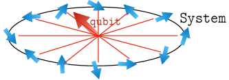
Figure 22: Sketch representing a qubit $\tt{q}$ (red arrow) coupled to an environment system $\tt{S}$ modeled by a quantum many-body spin chain (blue arrows). In the figure, homogeneous couplings are considered, however more general inhomogeneous (partial or local) couplings can be assumed.

We finally mention that the decoherence arising for the interaction with an environmental system is considered as the fundamental mechanism to understand the passage from quantum to classical behaviors (see, e.g., the review articles [756, 783] and references therein).

11.1 Setting of the problem

We consider a $d$-dimensional quantum many-body system ($\tt{S}$) of size $L^{d}$, whose Hamiltonian is the same as in Eq. (172),

$$\hat{H}_{\tt S}(w)=\hat{H}_{c}+w\hat{H}_{p}\,,$$ (245)

where, again, we assume that $\hat{H}_{c}$ is tuned at its critical point, the term $\hat{H}_{p}$ is the spatial integral of local operators, such that $[\hat{H}_{c},\hat{H}_{p}]\neq 0$, and the parameter $w$ drives a QT located at $w=0$. A paradigm example is the quantum Ising model (6) with $w\hat{H}_{p}$ corresponding to the longitudinal-field term, such that $\hat{H}_{p}=-\sum_{\bm{x}}\hat{\sigma}^{(1)}_{\bm{x}}$ and $w=h$. The parameter $w$ drives FOQTs along the $w=0$ line for any $g<g_{c}$. At the CQT point $g=g_{c}$, such term is one of the relevant perturbations driving the critical behavior, the other one being associated with the transverse-field term, identifying $\hat{H}_{p}=-\sum_{\bm{x}}\hat{\sigma}^{(3)}_{\bm{x}}$ and $w=g-g_{c}$.

In addition, we consider a qubit ($\tt{q}$) whose two-level Hamiltonian can be generally written as

$$\hat{H}_{q}=\sum_{k=\pm}\epsilon_{k}|k\rangle\langle k|=a\hat{I}_{2}+\tfrac{1}{2}s\,\hat{\Sigma}^{(3)}\,,$$ (246)

where $\hat{I}_{2}$ is the $2\times 2$ identity matrix, and the spin-1/2 Pauli operator $\hat{\Sigma}^{(3)}$ is associated with the two states $|\pm\rangle$ of the qubit, so that $\hat{\Sigma}^{(3)}|\pm\rangle=\pm|\pm\rangle$. The Hamiltonian eigenvalues are $\epsilon_{\pm}=a\pm s/2$, and $s=\epsilon_{+}-\epsilon_{-}$. The qubit is globally and homogeneously coupled to the many-body system, through the Hamiltonian term

$$\hat{H}_{\tt{qS}}=\big{(}u\,\hat{\Sigma}^{(3)}+v\,\hat{\Sigma}^{(1)}\big{)}\,\hat{H}_{p}\,,$$ (247)

where $\hat{H}_{p}$ is the operator appearing in Eq. (245). Putting all the terms together, we obtain the global Hamiltonian

$$\hat{H}=\hat{H}_{\tt S}+\hat{H}_{\tt q}+\hat{H}_{\tt{qS}}\,.$$ (248)

We consider a dynamic protocol arising from a sudden switching of the interaction $\hat{H}_{\tt{qS}}$ between the qubit and the many-body system, at time $t=0$, i.e., by instantaneously changing one or both of the control parameters $u$ and $v$ in Eq. (247), from zero to some finite value. More precisely:

• At $t=0$ the global system is prepared in the state

  $$|\Psi_{0}\rangle_{\tt{qS}}=|q_{0}\rangle_{\tt q}\otimes|\psi_{0}(w)\rangle_{\tt S}\,,$$ (249)

  where $|q_{0}\rangle_{\tt q}$ is a generic pure state of the qubit,

  $$|q_{0}\rangle_{\tt q}=c_{+}|+\rangle+c_{-}|-\rangle\,,\qquad|c_{+}|^{2}+|c_{-}|^{2}=1\,,$$ (250)

  and $|\psi_{0}(w)\rangle_{\tt S}$ is the ground state of the many-body system with Hamiltonian $\hat{H}_{\tt S}(w)$ .

• Then, the global wave function describing the quantum evolution for $t>0$ must be the solution of the Schrödinger equation

  $${{\rm d}\,|\Psi(t)\rangle\over{\rm d}t}=-i\,\hat{H}|\Psi(t)\rangle\,,\qquad|\Psi(t=0)\rangle\equiv|\Psi_{0}\rangle\,,$$ (251)

  where the global Hamiltonian $\hat{H}$ is the one reported in Eq. (248) and includes the interaction (247) between the qubit and the system (i.e., $\hat{H}_{\tt{qS}}\neq 0$, with the parameters $u$ and/or $v$ different from zero).

The above setting can be immediately extended to $N$-level systems coupled to an environment ${\tt S}$, and also to the case the initial qubit state is mixed, thus described by a nontrivial density matrix.

11.2 Qubit decoherence, work, and qubit-system energy exchanges

An interesting issue arising from the dynamics of the problem outlined above concerns the coherence properties of the qubit during the global quantum evolution. Starting from a pure state, the interaction with the many-body system may give rise to a loss of coherence of the qubit, depending on the properties of its density matrix

$$\rho_{\tt q}(t)={\rm Tr}_{\tt S}[\rho(t)]\,,$$ (252)

where ${\rm Tr}_{\tt S}[\>\cdot\>]$ denotes the trace over the ${\tt S}$-degrees-of-freedom of the global (pure) quantum state

$$\rho(t)=|\Psi(t)\rangle\langle\Psi(t)|\,,$$ (253)

with $|\Psi(t)\rangle$ given by the solution of Eq. (251). The coherence of the qubit during its quantum evolution can be quantified by its purity [see Sec. 6.3.3, Eq. (136)],

$${\rm Tr}\,\big{[}\rho_{\tt q}(t)^{2}\big{]}\equiv 1-D(t)\,,$$ (254)

where we have introduced the decoherence function $D$, such that $0\leq D\leq 1$. This function measures the quantum decoherence, quantifying the departure from a pure state. Indeed $D=0$ implies that the qubit is in a pure state, thus $D(t=0)=0$ initially. The other extreme value $D=1$ indicates that the qubit is totally unpolarized.

The initial quench, arising from turning on the interaction between the qubit $\tt{q}$ and the many-body system $\tt{S}$, can be also characterized via the quantum work $W$ done on the global system [594, 651]. After the quench, the energy is conserved during the global unitary evolution, thus we may only observe some energy flow between the qubit and the environment system. The work performed by changing the control parameters $u$ and $v$ does not generally have a definite value, while it can be defined as the difference of two projective energy measurements [594]. The first one at $t=0$ projects onto the eigenstates $|\Psi_{m}(i)\rangle$ of the initial Hamiltonian $\hat{H}_{i}=\hat{H}_{\tt q}+\hat{H}_{\tt S}$ with a probability $p_{m,i}$ given by the initial density matrix. The second energy measurement projects onto the eigenstates $|\Psi_{n}(f)\rangle$ of the post-quench Hamiltonian $\hat{H}_{f}=\hat{H}$ . The work probability distribution $P(W)$ associated with this quantum quench can be defined analogously to Eq. (187), so that the average quantum work $\langle W\rangle$ is given by

$$\langle W\rangle=\int dW\,W\,P(W)=\langle\Psi(t)|\hat{H}|\Psi(t)\rangle-\langle\Psi_{0}|\hat{H}_{\tt q}+\hat{H}_{\tt S}|\Psi_{0}\rangle=\langle\Psi_{0}|\hat{H}_{\tt{qS}}|\Psi_{0}\rangle\,,$$ (255)

where $|\Psi_{0}\rangle$ is the initial state in Eq. (249). An analogous expression can be derived for the average of the square work, obtaining $\langle W^{2}\rangle=\langle\Psi_{0}|\hat{H}_{\tt{qS}}^{2}|\Psi_{0}\rangle$. These relatively simple expressions for the first two moments of the work distribution do not extend to higher moments, whose expressions become more complicated, requiring the computation of the whole spectrum, due to the fact that $\hat{H}_{\tt{qS}}$ does not commute with the other Hamiltonian terms.

In order to study the qubit-system energy exchanges, one may consider the energy-difference distribution of the qubit, associated with two energy measurements at $t=0$ and at a generic time $t$. This is defined as

$$P_{\tt q}(U,t)=\!\sum_{n,a,b}\delta\big{[}U-(E_{qb}-E_{qa})\big{]}\,\big{|}\langle b,\psi_{n}|e^{-i\hat{H}t}|a,\psi_{0}\rangle\big{|}^{2}p_{a}\,.$$ (256)

Here $|b,\psi_{n}\rangle\equiv|b\rangle_{\tt q}\otimes|\psi_{n}\rangle_{\tt S}$, where $\{|a\rangle_{\tt q},\,|b\rangle_{\tt q}\}$ and $\{E_{{\tt q}a},E_{{\tt q}b}\}$ denote the eigenstates ($|\pm\rangle$) and eigenvalues of the qubit Hamiltonian $\hat{H}_{\tt q}$, while $\{|\psi_{n}\rangle_{\tt S}\}$ indicate the eigenstates of the system Hamiltonian $\hat{H}_{\tt S}$ , and $p_{\pm}=|c_{\pm}|^{2}$ are the probabilities of the initial qubit state at $t=0$. According to the definition (256), the average energy variation of the qubit reads

$$\langle U\rangle\equiv\int dU\,U\,P_{\tt q}(U,t)={\rm Tr}\big{[}\rho_{\tt q}(t)\,\hat{H}_{\tt q}\big{]}-{\rm Tr}\big{[}\rho_{\tt q}(t\!=\!0)\,\hat{H}_{\tt q}\big{]}\equiv E_{\tt q}(t)-E_{\tt q}(t\!=\!0)\,.$$ (257)

More general initial distributions may be also considered, for example associated with a bath at temperature $T$, replacing the initial density matrix $\rho_{0}=(|q\rangle_{\tt q}\otimes|\psi_{0}\rangle_{\tt S})\,({}_{\tt q}\langle q|\otimes{}_{\tt S}\langle\psi_{0}|)$ with the corresponding density matrices. A definition analogous to Eq. (256) associated with the qubit can be considered for the environment system [646].

11.3 Dynamic FSS ansatz for the qubit-system setup

The dynamic processes arising from the instantaneous turning on of the interaction term $\hat{H}_{\tt{qS}}$ can be described within a dynamic FSS framework, extending the frameworks outlined in Secs. 8 and 10, to take into account the interaction of the many-body system $\tt{S}$ with the qubit $\tt{q}$. Besides the scaling variable associated with the Hamiltonian parameter $w$ of the system, we also need to consider scaling variables associated with the other parameters of the global Hamiltonian $\hat{H}$ (i.e., $u$, $v$, and $s$). Since both the $u$- and the $v$-term are coupled to the operator $\hat{H}_{p}$, the corresponding scaling variables are expected to behave analogously to $w$ in the Hamiltonian $\hat{H}_{S}$. Therefore, at both CQTs and FOQTs of the system $\tt{S}$, assuming that $\delta E_{w}(L,w)$ is the energy variation arising from the longitudinal term $w$ coupled to $\hat{H}_{p}$, we introduce the scaling variables

$$\Phi_{w}\equiv{\delta E_{w}(L,w)\over\Delta(L)}\,,\qquad\Phi_{u}\equiv{\delta E_{w}(L,u)\over\Delta(L)}\,,\qquad\Phi_{v}\equiv{\delta E_{w}(L,v)\over\Delta(L)}\,,$$ (258)

where $\Delta(L)$ is the energy difference of the two lowest states of $\tt{S}$ at $w=0$. A scaling variable must also be associated with the energy difference $s$ of the eigenstates of the qubit Hamiltonian $\hat{H}_{\tt q}$. Since $s$ is a further energy scale of the problem, we define

$$\Lambda\equiv\frac{s}{\Delta(L)}\,.$$ (259)

Finally, the scaling variable $\Theta\equiv\Delta(L)\,t$ is associated with the time variable. The dynamic FSS limit that we consider is defined as the large-$L$ limit keeping the above scaling variables fixed. The above scaling variables can be adopted for both CQTs and FOQTs, with the appropriate, power-law or exponential, size dependence of $\Delta(L)$ and $\delta E_{w}(L,w)$, as discussed at the end of Sec. 5.1.

For the sake of clarity in the presentation, below we consider two limiting situations: (i) the simpler case $v=0$ and $u\neq 0$, for which $[\hat{H}_{\tt q},\hat{H}_{\tt{qS}}]=0$, and (ii) the more complicated case $u=0$ and $v\neq 0$, for which $[\hat{H}_{\tt q},\hat{H}_{\tt{qS}}]\neq 0$. In both cases, the dynamic FSS behavior of a generic observable is given by [645, 646]

$$O(t;L,w,u/v,s)\approx L^{y_{o}}\,{\cal O}(\Theta,\Phi_{w},\Phi_{u/v},\Lambda)\,,$$ (260)

where, again, $y_{o}$ is the RG dimension of $\hat{O}$ at CQTs ($y_{o}=0$ at FOQTs), and ${\cal O}$ is a dynamic FSS function. Note that, in the case (i) $v=0$, the dependence on the qubit spectrum $s$, and thus on the scaling variable $\Lambda$, disappears. Of course, the equilibrium FSS behavior must be recovered in the limit $u/v\to 0$.

11.4 Qubit decoherence functions

We now discuss the decoherence properties of the qubit in some detail. Results for the work associated with the initial quench and the energy flow between qubit and environment are reported in Ref. [646].

11.4.1 Central spin systems with $[\hat{H}_{\tt q},\hat{H}_{\tt{qS}}]=0$

The time evolution of the global system gets significantly simplified when $[\hat{H}_{\tt q},\hat{H}_{\tt{qS}}]=0$, i.e., when $v=0$ in Eq. (247), since the qubit exhibits pure dephasing in time, while the environment system evolves in two independent branches with the same Hamiltonian form and different fields [770, 771]. Indeed, the evolution of the global state can be written in terms of dynamic evolutions of the system $\tt{S}$ only, as

$$|\Psi(t)\rangle=e^{-i\epsilon_{+}t}c_{+}|+\rangle_{\tt q}\otimes|\phi_{w+u}(t)\rangle_{\tt S}+e^{-i\epsilon_{-}t}c_{-}|-\rangle_{\tt q}\otimes|\phi_{w-u}(t)\rangle_{\tt S}\,,$$ (261)

where

$$|\phi_{w\pm u}(t)\rangle_{\tt S}=e^{-i\hat{H}_{\tt S}(w\pm u)\,t}|\psi_{0}(w)\rangle_{\tt S}\,$$ (262)

are pure states of the environment system $\tt{S}$. Notable relations can be obtained focusing on the evolution of the qubit $\tt{q}$ only. The elements of its $2\times 2$ reduced density matrix, cf. Eq. (252), read:

$$\rho_{{\tt q},11}(t)=|c_{+}|^{2}\,,\qquad\rho_{{\tt q},22}(t)=|c_{-}|^{2}\,,\qquad\rho_{{\tt q},12}(t)=e^{-ist}c_{-}^{*}c_{+}\;{}_{\tt S}\langle\phi_{w-u}(t)|\phi_{w+u}(t)\rangle_{\tt S}=\rho_{{\tt q},21}(t)^{*}\,.$$ (263)

The decoherence function $D(t)$, cf. Eq. (254), can be written as

$$D(t)=2\,|c_{+}|^{2}\,|c_{-}|^{2}F_{D}\,,\qquad F_{D}\equiv 1-L_{D}(t)^{2}\,,\qquad L_{D}\equiv\big{|}{}_{\tt S}\langle\phi_{w-u}(t)|\phi_{w+u}(t)\rangle_{\tt S}\big{|}\,.$$ (264)

The function $F_{D}$, such that $0\leq F_{D}(t)\leq 1$ is a measure of quantum decoherence, quantifying the departure from a pure state: $F_{D}(t)=0$ implies that the qubit is in a pure state, while $F_{D}(t)=1$ indicates that the qubit is maximally entangled, corresponding to a diagonal density matrix $\rho_{\tt q}={\rm diag}\big{[}|c_{+}|^{2},|c_{-}|^{2}\big{]}$. Note that $D(t)$ does not depend on the spectrum of the qubit Hamiltonian $\hat{H}_{\tt q}$, and in particular on its parameter $s$.

The overlap function $L_{D}$ entering Eq. (264) can be interpreted as the fidelity, or the related Loschmidt echo, of the ${\tt S}$-states associated with two different quench protocols involving the isolated system ${\tt S}$. For both of them, the environment system starts from the ground state of the Hamiltonian $\hat{H}_{\tt S}(v)$ as $t=0$; then one considers, and compares using $L_{D}$, the quantum evolutions at the same $t$, arising from the sudden change of the Hamiltonian parameter $w$ to $w-u$ and to $w+u$. The dynamics FSS behavior of $L_{D}$ can be inferred from the theory developed in Sec. 8.4 at quench protocols:

$$L_{D}(t;L,w,u)\approx{\cal L}_{D}(\Theta,\Phi_{w},\Phi_{u})\,,$$ (265)

with ${\cal L}_{D}(\Theta,\Phi_{w},\Phi_{u}\!=\!0)=1$, and ${\cal L}_{D}(\Theta\!=\!0,\Phi_{w},\Phi_{u})=1$ .

Since $L_{D}(t;L,w,u)$ is an even function of $u$ and $D(t;L,w,0)=0$, we can write

$$D(t;L,w,u)=\tfrac{1}{2}u^{2}Q(t;L,w)+O(u^{4})\,,\qquad Q(t;L,w)=\frac{\partial^{2}D}{\partial u^{2}}\bigg{|}_{u=0}=2\,|c_{+}|^{2}\,|c_{-}|^{2}\,\frac{\partial^{2}F_{D}}{\partial u^{2}}\bigg{|}_{u=0}\,,$$ (266)

which also assumes an analytic behavior around $u=0$ (at finite $L$ and $t$). The function $Q$ quantifies the growth rate of decoherence in the limit of small qubit-environment coupling $u$, thus measuring the sensitivity of the coherence properties of the subsystems to $u$. The scaling behavior (265) allows us to derive the corresponding dynamic FSS of $Q$ as

$$Q(t;L,w)\approx\bigg{(}\frac{\partial\Phi_{u}}{\partial u}\bigg{)}^{2}{\cal Q}(\Theta,\Phi_{w})\,.$$ (267)

In the case of environment systems at CQTs, one has $\Phi_{u}=u\,L^{y_{w}}$, therefore it specializes into

$$Q(t;L,w)\approx L^{2y_{w}}{\cal Q}(\Theta,\Phi_{w})\,.$$ (268)

This scaling equation characterizes the amplified $O(L^{2y_{w}})$ rate of departure from coherence of the qubit. Indeed, in the case of systems out of criticality, one generally expects $Q\sim L^{d}$ and

$$2y_{w}=d+3-\eta>d\,.$$ (269)

For example, $\eta=1/4$ for 1$d$ quantum Ising-like chains, and $\eta\approx 0.036$ for 2$d$ quantum Ising systems (see Sec. 3.1). Therefore these results show a substantial enhancement of decoherence when the environment system is at a CQT, speeding up the decoherence by a large $O(L^{3-\eta})$ factor.

The rate enhancement of the qubit coherence loss is even more substantial at FOQTs, characterized by an exponentially large decoherence growth rate, related to the exponentially suppressed difference of the lowest levels in finite-size many-body systems at FOQTs. This occurs when the environment system ${\tt S}$ is at a FOQT and its BC are neutral, so that $\Delta(L)\sim e^{-cL^{d}}$. For example, one may consider quantum Ising systems at their FOQT line driven by $h$, identifying $w$ with $h$. In this case, since $\Phi_{u}\sim uL^{d}/\Delta(L)$, one has

$$\left({\partial\Phi_{u}\over\partial u}\right)^{2}\approx{L^{2d}\over\Delta(L)^{2}}\sim L^{2d}e^{2cL^{d}}\,,$$ (270)

to be compared again with the $O(L^{d})$ behavior expected for normal conditions, far from QTs. The corresponding scaling function ${\cal Q}$ can be computed by exploiting the two-level framework for the environment system at FOQTs [645]:

$${\cal Q}(\Theta,\Phi_{w})=2\,|c_{+}|^{2}\,|c_{-}|^{2}\,\frac{2\big{[}1-{\rm cos}(\Theta\sqrt{1+\Phi_{w}^{2}})\big{]}}{(1+\Phi_{w}^{2})^{2}}\,.$$ (271)

11.4.2 Central spin systems with $[\hat{H}_{\tt q},\hat{H}_{\tt{qS}}]\neq 0$

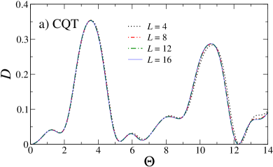
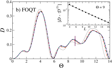
Figure 23: Decoherence function $D$ versus the rescaled time $\Theta$, for a qubit coupled to Ising spin-chain systems with PBC and of different lengths $L$ at the CQT, $g=g_{c}=1$ [left panel $(a)$], or at the FOQT, $g=0.9$ [right panel $(b)$]. All numerical data are for a qubit-system coupling realized through $u=0$ and $v\neq 0$ in Eq. (247), such that $[\hat{H}_{\tt q},\hat{H}_{\tt{qS}}]\neq 0$. We fix $\Phi_{w}=0.8$, $\Phi_{v}=1$, $\Lambda=0.5$, while the qubit is initialized with $c_{+}=\sqrt{2/3}$. The inset in the right panel $(b)$ shows numerical data for $\Theta=9$, supporting an exponential convergence to the prediction ${\cal D}^{(2l)}$ given by the two-level approximation for the Ising chain (thick brown line in the main frame). Adapted from Ref. [646].

Analogous scaling behaviors are conjectured in the more complex case (ii), $v\neq 0$, where $[\hat{H}_{\tt q},\hat{H}_{\tt{qS}}]\neq 0$ . In that case, the scaling functions are also expected to depend on the scaling variable $\Lambda$ in Eq. (259), associated with the energy spectrum of the qubit, in such a way that

$$D(t;L,w,v,s)\approx{\cal D}(\Theta,\Phi_{w},\Phi_{v},\Lambda)\,.$$ (272)

This dynamic FSS law has been numerically checked within the 1$d$ Ising chain at its CQT and along its FOQT line. The corresponding results, reported in Fig. 23, nicely support the conjectured behavior. In the case of environment systems ${\tt S}$ at FOQTs with neutral BC (as in the case of the figure), one can again exploit a two-level truncation of ${\tt S}$, thus leading to an effective model constituted by two coupled qubits, which is much simpler to handle [646].

Now, assuming analyticity for $D$ at $v=0$ and finite volume, and since $D\geq 0$, one expects an expansion analogous to Eq. (266),

$$D(t;L,w,v,s)=\tfrac{1}{2}v^{2}Q(t;L,w,s)+O(v^{3})\,,$$ (273)

which can be matched with the scaling behavior in Eq. (272), to obtain

$$Q(t;L,w,s)\approx\left({\partial\Phi_{v}\over\partial v}\right)^{2}{\cal Q}(\Theta,\Phi_{w},\Lambda)\,.$$ (274)

Like the case discussed in the previous Sec. 11.4.1, a power law arises when the environment system ${\tt S}$ is at a CQT, $Q\sim L^{2y_{w}}$. Conversely, an exponential law emerges at a FOQT (when considering neutral BC), such as $Q\sim\exp(bL^{d})$. One may compare these results with those expected when $\tt{S}$ is not close to a QT, for example for $g>g_{c}$ in the case of quantum Ising models, for which $Q$ is expected to increase as the volume of the system, i.e $Q\sim L^{d}$. A numerical validation of the above conjectures for the growth-rate function at CQTs, FOQTs, and far from QTs, within the quantum Ising chain, is reported in Fig. 24.

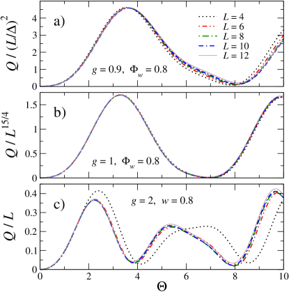
Figure 24: Scaling of the function $Q$ vs. the rescaled time $\Theta$, for three distinct situations of the Ising system ${\tt S}$: (a) on the FOQT line, for $g=0.9$; (b) at the CQT, for $g=g_{c}=1$; (c) in the disordered phase, for $g=2$. The evaluated growth-rate function quantifies the sensitivity of the qubit coherence to the coupling $v$. As in Fig. 23, we fix $\Lambda=0.5$ and $c_{+}=\sqrt{2/3}$. The longitudinal field $h=w$ has been chosen, without loss of generality, in such a way that $\Phi_{w}=0.8$ for panels (a) and (b), while $w=0.8$ in panel (c). Adapted from Ref. [646].

12 Master equations for open quantum systems

In Sec. 11 we have addressed the role of dissipative mechanisms on a single quantum spin ${\tt q}$ (the qubit), induced by the Hamiltonian coupling to another quantum system ${\tt S}$ (the environment). In that framework, the dynamics of the whole universe $\tt{q}+\tt{S}$ (qubit+environment) can be entirely described as a unitary evolution according to the Schrödinger equation with the global Hamiltonian (248). If one is interested in the analysis of the qubit alone, the time behavior of the corresponding reduced density matrix $\rho_{\tt q}(t)$ can be obtained by tracing over the environment system.

The above reasoning can be put on much more general grounds, by microscopically deriving a quantum master equation able to describe the continuous temporal evolution of a generic open quantum system itself (i.e., what have been previously called the qubit, and hereafter referred to as the system ${\tt s}$), without the necessity to keep track of the full environment dynamics (hereafter labelled with ${\tt E}$). In this section we give a brief overview on how to perform such derivation, concentrating on the so-called Gorini-Kossakowski-Lindblad-Sudarshan (GKLS) framework [784, 785]. Further details can be found, e.g., in Refs. [786, 787, 788, 789].

12.1 Evolution of closed and open quantum systems

We start by recalling some general properties of the temporal evolution of closed quantum systems. Under the hypothesis in which the system at time $t$ is in the pure state $|\psi(t)\rangle$, its time evolution is dictated by the usual Schrödinger equation. If the system Hamiltonian $\hat{H}$ is time-independent, its solution can be formally written as $|\psi(t)\rangle=\hat{U}(t,t_{0})|\psi(t_{0})\rangle$, where $\hat{U}(t,t_{0})=\exp[-i\hat{H}(t-t_{0})]$ is a unitary operator.  In the case the quantum system is in a statistical mixture, the state is generally written as a density matrix $\rho(t)$ and its time evolution is dictated by the von Neumann equation

$$\frac{{\rm d}\rho(t)}{{\rm d}t}=-i\big{[}\hat{H},\rho(t)\big{]}\,,\qquad\rho(t)=\hat{U}(t,t_{0})\,\rho(t_{0})\,\hat{U}^{\dagger}(t,t_{0})\equiv\mathbb{U}_{t_{0}\to t}\,\rho(t_{0})\,,$$ (275)

where $[\hat{A},\hat{B}]\equiv\hat{A}\hat{B}-\hat{B}\hat{A}$ denotes the commutator and $\mathbb{U}_{t_{0}\to t}$ is an operator on the operator space of the Hilbert space of the system, also named superoperator.

Now consider a system interacting with the environment (also known as a bath or reservoir). The most general Hamiltonian describing this situation is

$$\hat{H}=\hat{H}_{\tt s}+\hat{H}_{\tt E}+\hat{H}_{\tt sE}\,,$$ (276)

where $\hat{H}_{\tt s}$, $\hat{H}_{\tt E}$, and $\hat{H}_{\tt sE}$ respectively describe the system, the environment, and the interaction among the two. Usually the system-bath interaction is weak, so that the fast motion due to $\hat{H}_{0}\equiv\hat{H}_{\tt s}+\hat{H}_{\tt E}$ can be reasonably separated from the slow motion due to $\hat{H}_{\tt sE}$. Following this reasoning, one can exploit the interaction picture and define

$$\hat{\tilde{A}}_{\tt sE}(t)\equiv\hat{U}^{\dagger}(t)\,\hat{A}_{\tt sE}\,\hat{U}(t)\,,\qquad\hat{U}(t)=e^{-i\hat{H}_{\tt s}t}\otimes e^{-i\hat{H}_{\tt E}t}\,,$$ (277)

where $\hat{A}_{\tt sE}$ is a given operator acting on the whole system . Then, the von Neumann equation (275) for the full density matrix $\rho_{\tt sE}(t)$ reads

$$\frac{{\rm d}\tilde{\rho}_{\tt sE}(t)}{{\rm d}t}=-i\big{[}\hat{\tilde{H}}_{\tt sE}(t),\tilde{\rho}_{\tt sE}(t)\big{]}\,,$$ (278)

which is equivalent to

$$\tilde{\rho}_{\tt sE}(t)=\tilde{\rho}_{\tt sE}(0)-i\int_{0}^{t}{\rm d}\tau\,\big{[}\hat{\tilde{H}}_{\tt sE}(\tau),\tilde{\rho}_{\tt sE}(\tau)\big{]}\,,\qquad\tilde{\rho}_{\tt sE}(0)=\rho_{\tt sE}(0)\,.$$ (279)

Inserting the latter expression back into Eq. (278), we obtain

$$\frac{{\rm d}\tilde{\rho}_{\tt sE}(t)}{{\rm d}t}=-i\big{[}\hat{\tilde{H}}_{\tt sE}(t),\rho_{\tt sE}(0)\big{]}-\int_{0}^{t}{\rm d}\tau\,\Big{[}\hat{\tilde{H}}_{\tt sE}(t),\big{[}\hat{\tilde{H}}_{\tt sE}(\tau),\tilde{\rho}_{\tt sE}(\tau)\big{]}\Big{]}\,.$$ (280)

Now, tracing over the degrees of freedom of ${\tt E}$, and using the fact that

$${\rm Tr}_{\tt E}\big{[}\tilde{\rho}_{\tt sE}\big{]}={\rm Tr}_{\tt E}\big{[}\hat{U}^{\dagger}\,\rho_{\tt sE}\,\hat{U}\big{]}=\hat{U}^{\dagger}_{\tt s}\>{\rm Tr}_{\tt E}\big{[}U^{\dagger}_{\tt E}\,\rho_{\tt sE}\,\hat{U}_{\tt E}\big{]}\,\hat{U}_{\tt s}=\hat{U}^{\dagger}_{\tt s}\,{\rm Tr}_{\tt E}\big{[}\rho_{\tt sE}\big{]}\,\hat{U}_{\tt s}=\tilde{\rho}_{\tt s}\,,$$ (281)

we obtain the following integro-differential equation for $\rho_{\tt s}$:

$$\frac{{\rm d}\tilde{\rho}_{\tt s}(t)}{{\rm d}t}=-i\,{\rm Tr}_{\tt E}\Big{\{}\big{[}\hat{\tilde{H}}_{\tt sE}(t),\rho_{\tt sE}(0)\big{]}\Big{\}}-\int_{0}^{t}{\rm d}\tau\,{\rm Tr}_{\tt E}\Big{\{}\Big{[}\hat{\tilde{H}}_{\tt sE}(t),\big{[}\hat{\tilde{H}}_{\tt sE}(\tau),\tilde{\rho}_{\tt sE}(\tau)\big{]}\Big{]}\Big{\}}\,.$$ (282)

12.2 Markovian quantum master equations

Equation (282) is exact but practically useless, being extremely difficult to handle. In order to proceed further with the derivation of a simpler master equation for $\rho_{\tt s}(t)$, two important approximations are usually invoked:

• Born approximation. It consists in taking an environment ${\tt E}$ much larger than the system ${\tt s}$, so that it is practically unaffected by the interactions with the system.

• Markov approximation. The environment ${\tt E}$ may acquire information on the system, which can also flow back (at least in part) into ${\tt s}$. One generally assumes that the state of the environment at time $t_{0}$ is essentially unaffected by the history of the system. This implies that the information flow is one-way, from the system to the environment $\tt{s}\to\tt{E}$ (and not vice-versa). More precisely, the knowledge of the system density matrix $\rho_{\tt s}(t_{0})$ at a given time $t_{0}$ is sufficient to determine $\rho_{\tt s}(t)$ at any time $t>t_{0}$.

In practice, one starts by assuming that, at time $t=0$, the system and the environment are uncorrelated:

$$\rho_{\tt sE}(0)=\rho_{\tt S}(0)\otimes\rho_{\tt E}(0)\,,$$ (283)

thus the interaction Hamiltonian $\hat{H}_{\tt sE}$ does not significantly affect the global ground state of the whole universe (i.e., system+environment). We also suppose that

$${\rm Tr}_{\tt E}\Big{\{}\big{[}\hat{\tilde{H}}_{\tt sE}(t),\rho_{\tt sE}(0)\big{]}\Big{\}}=0\,,$$ (284)

thus eliminating the first term in the right-hand side of Eq. (282). In fact it can be shown that, if this is not the case, one could always redefine $\hat{H}_{\tt s}$ and $\hat{H}_{\tt sE}$, while keeping the global Hamiltonian $\hat{H}$ constant, in order to fulfill Eq. (284).

Within the Born approximation, the system-bath coupling is so weak and the reservoir so large that its state is essentially unaffected by the interaction $\hat{H}_{\tt sE}$. In practice, this amounts to assuming that correlations between the system and the bath remain negligible at all times, therefore

$$\tilde{\rho}_{\tt sE}(t)\approx\tilde{\rho}_{\tt s}(t)\otimes\tilde{\rho}_{\tt E}\,,\qquad\quad\mbox{since}\quad\rho_{\tt E}\equiv\rho_{\tt E}(t)\approx\rho_{\tt E}(0)\,.$$ (285)

Of course, this assumption relies on the fact that the bath equilibrates on a time scale $\tau_{\tt E}$ much faster than that of the system evolution $\tau_{\tt s}$, namely $\tau_{\tt s}\gg\tau_{\tt E}$. Using Eq. (284) and plugging (285) in Eq. (282), we obtain

$$\frac{{\rm d}\tilde{\rho}_{\tt s}(t)}{{\rm d}t}=-\int_{0}^{t}{\rm d}\tau\,{\rm Tr}_{\tt E}\Big{\{}\Big{[}\hat{\tilde{H}}_{\tt sE}(t),\big{[}\hat{\tilde{H}}_{\tt sE}(\tau),\tilde{\rho}_{\tt s}(\tau)\otimes\tilde{\rho}_{\tt E}\big{]}\Big{]}\Big{\}}\,.$$ (286)

The Markov approximation guarantees that one can safely substitute $\tilde{\rho}_{\tt s}(\tau)\to\tilde{\rho}_{\tt s}(t)$ in Eq. (286), meaning that the density matrix $\tilde{\rho}_{\tt s}$ remains approximately constant over all the time interval $0\leq\tau\leq t$. As a consequence, we obtain

$$\frac{{\rm d}\tilde{\rho}_{\tt s}(t)}{{\rm d}t}=-\int_{0}^{t}{\rm d}\tau\,{\rm Tr}_{\tt E}\Big{\{}\Big{[}\hat{\tilde{H}}_{\tt sE}(t),\big{[}\hat{\tilde{H}}_{\tt sE}(\tau),\tilde{\rho}_{\tt s}(t)\otimes\tilde{\rho}_{\tt E}\big{]}\Big{]}\Big{\}}\,,$$ (287)

thus reducing to an equation of motion for the system ${\tt s}$ that is simply differential (and no longer integro-differential), since $\tilde{\rho}_{\tt s}$ in the right-hand side has not to be integrated in time. Equation (287) is known as the Redfield master equation.

In fact, the Redfield equation is still non-Markovian, as it retains memory of the initial-state preparation of the system, $\rho_{\tt s}(0)$. To obtain a Markovian equation, a coarse graining in time has to be performed, by extending the upper limit of the integration to infinity, with no real change in the outcome:

$$\frac{{\rm d}\tilde{\rho}_{\tt s}(t)}{{\rm d}t}=-\int_{0}^{+\infty}{\rm d}\tau\,{\rm Tr}_{\tt E}\Big{\{}\Big{[}\hat{\tilde{H}}_{\tt sE}(t),\big{[}\hat{\tilde{H}}_{\tt sE}(t-\tau),\tilde{\rho}_{\tt s}(t)\otimes\tilde{\rho}_{\tt E}\big{]}\Big{]}\Big{\}}\,,$$ (288)

where, for the sake of convenience, we changed the integral variable $\tau\to t-\tau$. The two-step approximation described in Eqs. (287) and (288) is known as the Markov approximation. The final result has been thus derived for weak coupling and quickly decaying reservoir correlations (i.e., memoryless dynamics).

12.2.1 Lindblad master equations

Unfortunately the master equation (288), holding under the Born-Markov approximation, does not warrant the positivity of $\rho_{\tt s}(t)$ at a generic time $t$, sometimes giving rise to density matrices that are non-positive. To ensure complete positivity, one further approximation is needed:

• Secular approximation. As we shall see below, it involves discarding fast oscillating terms in the Redfield master equation, which can be neglected if the characteristic time of the system is much larger than that of the bath. In the context of quantum optics, this is equivalent to the so-called rotating wave approximation, which consists in dropping all fast oscillating frequencies of a combined atom-photon system near the electromagnetic resonance.

To be explicit, we decompose the interaction Hamiltonian $\hat{H}_{\tt sE}$ in terms of operators of the system and of the environment, according to

$$\hat{H}_{\tt sE}=\sum_{\alpha}\hat{S}_{\alpha}\otimes\hat{E}_{\alpha}\,,$$ (289)

where $\hat{S}_{\alpha}$ and $\hat{E}_{\alpha}$ are Hermitian operators acting on the system ${\tt s}$ and the environment ${\tt E}$, respectively. Assuming that $\hat{H}_{\tt s}$ has a discrete spectrum, one can define the eigenoperators of the system as

$$\hat{S}_{\alpha}(\omega)=\sum_{\epsilon,\epsilon^{\prime},\,\epsilon^{\prime}-\epsilon=\omega}\,\hat{\Pi}(\epsilon)\,\hat{S}_{\alpha}\,\hat{\Pi}(\epsilon^{\prime})\,,$$ (290)

where the sum is extended over the couples of eigenvalues of $\hat{H}_{\tt s}$ whose difference is equal to $\omega$, while $\hat{\Pi}(\epsilon)$ is the projector on the corresponding $\epsilon$-th eigenspace. These operators satisfy the properties

$$\sum_{\omega}\hat{S}_{\alpha}(\omega)=\hat{S}_{\alpha}\,,\qquad\hat{S}^{\dagger}_{\alpha}(\omega)=\hat{S}_{\alpha}(-\omega)\,,\qquad\hat{\tilde{S}}_{\alpha}(\omega)=e^{-i\omega t}\hat{S}_{\alpha}(\omega)\,,$$ (291a)

$$\big{[}\hat{H}_{\tt s},\hat{S}_{\alpha}(\omega)\big{]}=-\omega\hat{S}_{\alpha}(\omega)\,,\qquad\big{[}\hat{H}_{\tt s},\hat{S}^{\dagger}_{\alpha}(\omega)\big{]}=\omega\hat{S}^{\dagger}_{\alpha}(\omega)\,.$$ (291b)

Using them, the interaction Hamiltonian can be written in the interaction picture as

$$\hat{\tilde{H}}_{\tt sE}(t)=\sum_{\alpha,\omega}e^{-i\omega t}\hat{S}_{\alpha}(\omega)\otimes\hat{\tilde{E}}_{\alpha}(t)=\sum_{\alpha,\omega}e^{i\omega t}\hat{S}^{\dagger}_{\alpha}(\omega)\otimes\hat{\tilde{E}}^{\dagger}_{\alpha}(t)\,.$$ (292)

Now, expanding the commutators in the Redfield equation (288) and using the expression (292), it is possible to obtain the following:

$$\frac{{\rm d}\tilde{\rho}_{\tt s}(t)}{{\rm d}t}=\sum_{\omega,\omega^{\prime}}\sum_{\alpha,\beta}\left\{e^{i(\omega^{\prime}-\omega)t}\,\Gamma_{\alpha,\beta}(\omega)\,\big{[}\hat{S}_{\beta}(\omega)\tilde{\rho}_{\tt S}(t),\hat{S}^{\dagger}_{\alpha}(\omega^{\prime})\big{]}+{\rm h.c.}\right\}\,.$$ (293)

The quantity $\Gamma_{\alpha,\beta}(\omega)$ denotes the one-sided Fourier transform of the reservoir two-point correlation functions,

$$\Gamma_{\alpha,\beta}(\omega)=\int_{0}^{\infty}{\rm d}\tau\,e^{i\omega\tau}\>{\rm Tr}_{\tt E}\,\Big{[}\hat{\tilde{E}}_{\alpha}^{\dagger}(t)\,\hat{\tilde{E}}_{\beta}(t-\tau)\,\rho_{\tt E}\,\Big{]}\,.$$ (294)

Note that $\Gamma$ does not depend on time $t$ since, under the hypothesis of a stationary reservoir, its correlation functions are homogeneous in time and the argument of the trace can be shifted into: $\big{[}\hat{\tilde{E}}_{\alpha}^{\dagger}(\tau)\,\hat{\tilde{E}}_{\beta}(0)\,\rho_{\tt E}\big{]}$.

At this point, we can invoke the secular approximation. Given the characteristic evolution time $\tau_{\tt s}$ of the system (that is, the time scale over which the properties of ${\tt s}$ change appreciably), this is generally of the order of $\tau_{\tt s}\approx|\omega^{\prime}-\omega|^{-1}$, for $\omega^{\prime}\neq\omega$. If $\tau_{\tt s}\gg\tau_{\tt E}$ (holding for weak system-bath couplings), the terms in (293) involving large energy differences ($\omega^{\prime}\neq\omega$) will be fastly oscillating, thus averaging out to zero. According to the secular approximation, only the resonant terms $\omega=\omega^{\prime}$ significantly contribute to the dynamics, while all the others are neglected, so that the sum over $\omega^{\prime}$ and the imaginary exponential in Eq. (293) drop.

We finally decompose the environment correlation matrix $\Gamma$ into its Hermitian and non-Hermitian parts, $\Gamma_{\alpha,\beta}(\omega)=\tfrac{1}{2}\gamma_{\alpha,\beta}(\omega)+i\pi_{\alpha,\beta}(\omega)$, with

$$\gamma_{\alpha,\beta}(\omega)=\Gamma_{\alpha,\beta}(\omega)+\Gamma^{*}_{\beta,\alpha}(\omega)\,,\qquad\quad\pi_{\alpha,\beta}(\omega)=\frac{1}{2i}\Big{[}\Gamma_{\alpha,\beta}(\omega)-\Gamma^{*}_{\beta,\alpha}(\omega)\Big{]}\,.$$ (295)

With these definitions, it is possible to separate the Hermitian and non-Hermitian parts of the dynamics ruled by Eq. (293) and then transform back to the Schrödinger picture, to obtain

$$\frac{{\rm d}\rho_{\tt s}(t)}{{\rm d}t}=-i\big{[}\hat{H}+\hat{H}_{Ls},\rho_{\tt s}(t)\big{]}+\mathbb{D}[\rho_{\tt s}(t)]\,,$$ (296)

where the first term in the right-hand side provides the coherent Hamiltonian dynamics of the system. The second term, given by the superoperator

$$\mathbb{D}[\rho_{\tt s}(t)]=\sum_{\omega}\sum_{\alpha,\beta}\gamma_{\alpha,\beta}\Big{[}\hat{S}_{\beta}(\omega)\,\rho_{\tt s}(t)\,\hat{S}^{\dagger}_{\alpha}(\omega)-\frac{1}{2}\big{\{}\hat{S}^{\dagger}_{\alpha}(\omega)\,\hat{S}_{\beta}(\omega),\rho_{\tt s}(t)\big{\}}\Big{]}\,,$$ (297)

with $\{\hat{A},\hat{B}\}\equiv\hat{A}\hat{B}+\hat{B}\hat{A}$ denoting the anticommutator, accounts for the interaction between the system and the environment. Note that the Hamiltonian dynamics becomes influenced by an additional term

$$\hat{H}_{Ls}=\sum_{\omega}\sum_{\alpha,\beta}\hat{\pi}_{\alpha,\beta}(\omega)\,\hat{S}^{\dagger}_{\alpha}(\omega)\,\hat{S}_{\beta}(\omega)\,,$$ (298)

usually called Lamb-shift Hamiltonian, whose role is to renormalize the system energy levels due to the interaction with the environment.

Since $\gamma_{\alpha,\beta}(\omega)$ can be seen as the Fourier transform of the positive function ${\rm Tr}\,[\hat{E}^{\dagger}_{\alpha}(\tau)\,\hat{E}_{\beta}(0)\,\rho_{\tt E}]$, the matrix composed of its entries can be diagonalized. Thus we finally arrive at the GKLS master equation (hereafter shortened into the Lindblad master equation), given by Eq. (296) with the dissipator

$$\mathbb{D}[\rho_{\tt s}(t)]=\sum_{\omega}\sum_{\alpha}\gamma_{\alpha}\Big{[}\hat{L}_{\alpha}(\omega)\,\rho_{\tt s}(t)\,\hat{L}^{\dagger}_{\alpha}(\omega)-\frac{1}{2}\big{\{}\hat{L}^{\dagger}_{\alpha}(\omega)\,\hat{L}_{\alpha}(\omega),\rho_{\tt s}(t)\big{\}}\Big{]}\,.$$ (299)

The operators $\hat{L}_{\alpha}(\omega)$, usually referred to as the Lindblad jump operators, are obtained through a unitary transformation which diagonalizes $\gamma_{\alpha,\beta}(\omega)$, while $\gamma_{\alpha}\geq 0$ are its eigenvalues. 

The Lindblad master equation (296)-(299) can be shown to be the most general form of continuous-time evolutor which guarantees that its solution $\rho(t)$ is a well-defined density operator at all times, preserving its trace and complete positivity. More precisely, it defines the Liouvillian superoperator $\mathbb{L}$,

$$\frac{{\rm d}\rho(t)}{{\rm d}t}=\mathbb{L}[\rho(t)]\,,\qquad\rho(t)=e^{\mathbb{L}t}\rho(0)\,,$$ (300)

which represents the most general generator of a quantum dynamical semigroup, i.e., a continuous, one-parameter family of dynamical maps satisfying the semigroup property: $\mathbb{L}(t_{1})\,\mathbb{L}(t_{2})=\mathbb{L}(t_{1}+t_{2})$, $t_{1},t_{2}\geq 0$.

12.2.2 Local Lindblad master equations

Finding suitable expressions for the jump operators $\hat{L}_{\alpha}(\omega)$, the Lamb-shift correction to the Hamiltonian, and the couplings $\gamma_{\alpha}$ entering Eqs. (296)-(299) can be a laborious problem, especially for complex systems. In most situations, local system-bath coupling schemes are assumed from phenomenological grounds, so that typically the $\hat{H}_{Ls}$ correction is neglected, while the Lindblad operators $\hat{L}_{j}$ are taken as acting on an appropriate spatial coordinate (e.g., a single site of a quantum lattice model). This represents the standard framework for quantum many-body systems, giving reliable results for quantum optical devices [790]. In such context, one of the techniques that have been employed is the Keldysh path-integral approach [791, 790]. Several paradigmatic examples presented in the next sections of this review are based on local system-environment couplings. However we wish to warn the reader that, strictly speaking, the eigenoperators $\hat{S}_{\alpha}(\omega)$ of the system (and, consequently, the jump operators) are nonlocal. As a result, the local approach may lead to contradictory results and to a violation of the second principle of thermodynamics [792].

More in detail, a local shape can be recovered only after assuming that there is no coupling between the different subsystems (e.g., the sites) composing ${\tt s}$. On the other hand, for generic many-body Hamiltonians, there is no reason to assume that the local approximation is valid. The crucial point of the derivation leading to Eqs. (296)-(299) is the spectral decomposition of $\hat{H}_{\tt s}$, which is required to find the eigenoperators $\hat{S}_{\alpha}(\omega)$. For interacting quantum many-body systems, this can be an extremely hard task, therefore the full microscopic derivation of the master equation is rarely used in physical situations, apart from very specific cases [793]. Among them we mention the infinite bosonic tight-binding chain [794] and the class of quadratic quantum many-body systems [795], which can be however mapped into free quasiparticle systems.

12.3 Steady states

The long-time dynamics described by a given master equation deals with the possible convergence towards a time-independent steady state: $\lim_{t\to\infty}\rho(t)=\rho_{ss}$. This is defined as a state which is annihilated by the Liouvillian superoperator (300),

$$\mathbb{L}[\rho_{ss}]=0\,.$$ (301)

It can be proven that every Lindblad master equation admits at least one steady state. Determining whether this steady state is unique or not is a subtle issue: although a number of theorems have been proposed to characterize the conditions under which a unique steady state is expected, a conclusive statement on this subject has not been reached so far [796, 797, 798, 799, 800].

Nevertheless, an important result put forward by Spohn [801] states that, if the set of Lindblad operators $\{\hat{L}_{i}\}$ is self-adjoint and its bicommutant $\{\hat{L}_{i}\}^{\prime\prime}$ equals the entire operator space, then the steady state is unique . This ensures that a relevant class of many-body Lindblad master equations admits a unique steady state, as for quadratic fermionic or bosonic systems linearly coupled to an environment modeled by a set of independent thermal baths [795]. Other many-body systems can be proven to belong to this category, such as those made by finite-dimensional subsystems, and described by local Lindblad master equations in which the jump operators are associated either to raising or to lowering operators [800]. Nonetheless, even if one is sure that the steady state is unique, there is no reason to believe that the relaxation process must be of the thermal kind: the open-system dynamics may originate nontrivial nonequilibrium steady states.

12.4 Validity of the Born-Markov approximations

We conclude this overview on open quantum systems by mentioning that, while justified in certain contexts, the approximations leading to the Redfield and the Lindblad master equations are not necessarily satisfied in physical situations. In particular, they fail when the system-environment interaction is not very weak and leads to long-lasting and non-negligible correlations [786]. This is the most common scenario in several realistic cases (e.g., in solid-state systems), where the open-system dynamics is inevitably non-Markovian and is affected by important memory effects.

Although worth being investigated, we will not pursue further in this direction, due to the lack of substantial results in the many-body context (see however Sec. 13.6, where we discuss a different system-bath interaction scheme, in which the environment is modeled by an infinite set of harmonic oscillators, that may lead to rather different physical behaviors). The reader who is interested in further details on the mathematical derivation of such situations and of non-Markovianity witnesses can have a look at Refs. [787, 802, 803, 804], based on a quantum-information perspective.

13 Dissipative perturbations at quantum transitions

In this section we discuss the dynamics of a many-body system in proximity of a QT, in the presence of dissipative perturbations arising from the interaction with the environment. We consider a class of dissipative mechanisms whose dynamics can be effectively described through a Lindblad master equation governing the time evolution of the system’s density matrix [786, 787] (see Sec. 12). Within this framework, the evolution of the density matrix $\rho(t)$ of the many-body system is described by the Lindblad master equation [786]

$${{\rm d}\rho\over{\rm d}t}={\cal L}[\rho]:=-i\big{[}\hat{H},\rho\big{]}+u\,{\mathbb{D}}[\rho]\,,\qquad{\mathbb{D}}[\rho]=\sum_{o}{\mathbb{D}}_{o}[\rho]\,,$$ (302a)

where $${\cal L}[\rho] {\mathbb{D}}_{o} u>0 {\mathbb{D}}_{o}[\rho]$$ represents the generator of the dissipative dynamics, its first term provides the coherent driving, while its second term accounts for the coupling to the environment. Its form depends on the nature of the dissipation arising from the interaction with the bath, which is effectively described by a set of dissipators , and a global coupling strength . In the case of systems weakly coupled to Markovian baths, the trace-preserving superoperator can be generally written as [785, 784]

$${\mathbb{D}}_{o}[\rho]=\hat{L}_{o}\rho\hat{L}_{o}^{\dagger}-\tfrac{1}{2}\big{(}\rho\,\hat{L}_{o}^{\dagger}\hat{L}_{o}+\hat{L}_{o}^{\dagger}\hat{L}_{o}\rho\big{)}\,,$$ (302b)

where $\hat{L}_{o}$ is the Lindblad jump operator associated with the system-bath coupling scheme. In the following discussion we restrict to homogeneous dissipation mechanisms, preserving translational invariance, as depicted, for example, in Fig. 25. In quantum optical implementations, the conditions leading to Eqs. (302) are typically satisfied [790], therefore this formalism constitutes the standard choice for theoretical investigations of this kind of systems.

It is worth mentioning that an increasing interest is developing on the study of driven-dissipative QTs in many-body systems governed by the Lindblad master equation (302), i.e., on QTs that may emerge in the steady-state density matrix of the dynamics generated by the Liouvillian ${\cal L}[\rho]$. A number of works recently started to tackle this problem under different perspectives, both theoretical (see, e.g., Refs. [805, 806, 807, 808, 809, 810, 811, 812, 813, 814, 815, 816]) and experimental (see, e.g., Refs. [817, 818, 585]). However, we will not pursue this topic further in this review.

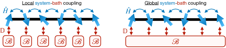
Figure 25: Sketch of a quantum spin-chain model locally and globally coupled to external baths. Neighboring spins are coupled through a coherent Hamiltonian $\hat{H}$ (bidirectional blue arrows). Each spin is also homogeneously and weakly coupled to some external bath ${\cal B}$ via a set of dissipators $\mathbb{D}$ (vertical red arrows), whose effect is to induce incoherent dissipation. The environment can be modeled either as a sequence of local independent baths, each for any spin of the chain (left drawing), or as a single common bath to which each spin is supposed to be uniformly coupled (right drawing). Adapted from Ref. [673].

13.1 Quench protocols to test coherent and dissipative dynamics

The interplay between the critical coherent dynamics and the dissipative mechanisms can be addressed within a simple dynamic protocol. We assume again that the many-body Hamiltonian can be written as in Eq. (172), i.e., $\hat{H}(w)=\hat{H}_{c}+w\hat{H}_{p}$, where the term associated with the Hamiltonian parameter $w$ represents a relevant perturbation to the critical Hamiltonian $\hat{H}_{c}$. We consider the following protocol:

• The system is prepared in the ground state of the Hamiltonian in Eq. (172), associated with a given value $w_{i}$, that is, the initial state at $t=0$ is $\rho(0)=|\Psi_{0}(w_{i})\rangle\langle\Psi_{0}(w_{i})|$. Alternatively, one may consider an initial state at temperature $T$, described by the Gibbs distribution $\propto\exp[-\hat{H}(w_{i})/T]$.

• Then, the dissipative interaction with the environment is suddenly turned on, so that the system evolves according to the Lindblad master equation (302) with $u>0$. One may also allow for an instantaneous quench of the Hamiltonian parameter $w$, from $w_{i}$ to $w\neq w_{i}$.

The approach to the asymptotic stationary states is generally controlled by the Liouvillian gap $\Delta_{\cal L}$ associated with the generator ${\cal L}$ of the dissipative dynamics [see Eq. (302a)] [786, 787, 819, 813, 820]. In fact, the asymptotic stationary state is provided by the eigenstate of ${\cal L}$ with vanishing eigenvalue, $\Lambda_{0}=0$, while all the other eigenstates have eigenvalues $\Lambda_{i}$ with negative real part [i.e., ${\rm Re}\,(\Lambda_{i})<0$ for any $i>0$]. The convergence to the stationary state is ruled by the Liouvillian eigenvalue with the largest nonzero real part, that is,

$$\Delta_{\cal L}=-{\rm Max}_{i>0}\,{\rm Re}\,(\Lambda_{i})\,.$$ (303)

The dissipator ${\mathbb{D}}=\sum_{o}{\mathbb{D}}_{o}$ can drive the system to a steady state, which is generally noncritical, even when the Hamiltonian parameters are critical. However, one can identify a dynamic regime where the dissipation is sufficiently small to compete with the coherent evolution driven by the critical Hamiltonian, leading to dynamic scaling behaviors somehow controlled by the universality class of the QT of the isolated system. This occurs within a low-dissipation regime, where the decay rate of the dissipation is comparable with the ground-state energy gap of the Hamiltonian. Such low-dissipation regime naturally emerges within dynamic scaling frameworks, also involving the strength $u$ of the coupling with the dissipators in the Lindblad equation [574, 821]. Analogously to the scaling laws of closed systems at QTs, the dynamic scaling behavior in the presence of dissipation is expected to be universal, i.e., largely independent of the microscopic details.

We remind the reader that hereafter we only focus on situations close to a QT point for the corresponding closed system, so that the dissipation acts as a perturbation. On the other hand, we are not going to address nonequilibrium phenomena leading to novel critical behaviors and/or QTs in the steady states, which are genuinely induced by the mutual interplay of the unitary and the dissipative dynamics.

Other different aspects concerning localized dissipative interactions with the environment have been discussed in the literature (see, e.g., Refs. [822, 823, 824, 825, 819, 826, 827, 828, 829, 820, 830, 831, 832, 833, 834]), and, in particular, for the case of quantum Ising-like and fermionic chains with dissipative interactions at the ends of the chain [822, 823, 824, 825, 819, 826, 820, 834]. Hereafter we will not deal with such issues.

13.2 Quantum thermodynamics of the dynamic process

The out-of-equilibrium quantum dynamics associated with the above-mentioned protocol can be monitored by considering standard observables, such as those defined in Eqs. (174-176). Other useful quantities are related to the thermodynamics of the process, such as the average work and heat characterizing the quantum thermodynamic properties of the out-of-equilibrium dynamics associated with the dissipative interaction with the environment.

The first law of thermodynamics describing the energy flows of the global system, including the environment, can be written as [835, 836, 837]

$${{\rm d}E_{s}\over{\rm d}t}=W^{\prime}(t)+Q^{\prime}(t)\,,$$ (304)

where $E_{s}$ is the average energy of the open system,

$$E_{s}\equiv{\rm Tr}\,\big{[}\rho(t)\,\hat{H}(t)\big{]}\,,$$ (305)

and

$$W^{\prime}(t)\equiv{{\rm d}W\over{\rm d}t}={\rm Tr}\bigg{[}\rho(t)\,{{\rm d}\hat{H}(t)\over{\rm d}t}\bigg{]}\,,\qquad Q^{\prime}(t)\equiv{{\rm d}Q\over{\rm d}t}={\rm Tr}\bigg{[}{{\rm d}\rho(t)\over{\rm d}t}\,\hat{H}(t)\bigg{]}\,,$$ (306)

with $W$ and $Q$ respectively denoting the average work done on the system and the average heat interchanged with the environment.

In the quench protocol outlined in Sec. 13.1, a nonvanishing work is only done at $t=0$, when the longitudinal-field parameter suddenly changes from $w_{i}$ to $w$. After that, the Hamiltonian is kept fixed for any $t>0$, therefore the average work is simply given by the static expectation value

$$W=\langle\Psi_{0}(w_{i})|\hat{H}(w)-\hat{H}(w_{i})|\Psi_{0}(w_{i})\rangle=(w-w_{i})\,\langle\Psi_{0}(w_{i})|\hat{H}_{p}|\Psi_{0}(w_{i})\rangle\,.$$ (307)

Note that the average work of this protocol is the same of that arising at sudden quenches of closed systems, already discussed in Sec. 8.5. On the other hand, the heat interchange with the environment is strictly related to the dissipative mechanism. Indeed one can easily derive the relation

$$Q^{\prime}(t)=u\,{\rm Tr}\big{[}{\mathbb{D}}[\rho]\,\hat{H}(t)\big{]}\,,$$ (308)

by substituting the right-hand side of the Lindblad equation (302a) into the expression (306).

13.3 Dynamic scaling laws in the presence of homogeneous dissipation

To account for the role of the dissipators, the dynamic FSS theory outlined in the previous sections has to be extended. In fact, the effect of a sufficiently low dissipation can be taken into account by adding a further dependence on the variable associated with $u$ in the dynamic homogeneous laws (178b). For example, one may write 

$$G_{12}(t,{\bm{x}};L,w_{i},w,u)\equiv\big{\langle}\hat{O}_{1}({\bm{x}}_{1})\,\hat{O}_{2}({\bm{x}}_{2})\big{\rangle}_{t}\approx b^{-\varphi_{12}}\,{\cal G}_{12}(b^{-\zeta}t,b^{-1}{\bm{x}},b^{-1}L,b^{y_{w}}w_{i},b^{y_{w}}w,b^{\zeta}u)\,,$$ (309)

in which we added the argument $b^{\zeta}u$, where $\zeta$ is a suitable exponent, to ensure the substantial balance (thus competition) with the critical coherent driving. As argued in Refs. [838, 574], the exponent $\zeta$ appropriate for homogeneous dissipation should generally coincide with the dynamic exponent $z$. This is a natural conjecture, due to the fact that the parameter $u$ in Eq. (302a) plays the role of a decay rate, i.e., of an inverse relaxation time for the associated dissipative process [786], and any relevant time scale at a QT scales as $\Delta^{-1}$.

As usual, to derive dynamic FSS laws one can set $b=L$, such that

$$G_{12}(t,{\bm{x}};L,w_{i},w,u)\approx L^{-\varphi_{12}}\,{\cal G}_{12}(\Theta,{\bm{X}},\Phi_{i},\Phi,\Gamma)\,,$$ (310)

where the scaling variables $\Theta,{\bm{X}},\Phi,\delta_{w}$ (or $\Phi_{i}$) have been defined within the dynamic FSS of closed systems, cf. Eq. (182), i.e., $\Theta=L^{-z}t$, ${\bm{X}}={\bm{x}}/L$, $\Phi=L^{y_{w}}w$, and $\delta_{w}={w/w_{i}}-1$, while the new scaling variable associated with the dissipation is given by

$$\Gamma\equiv L^{z}\,u\,.$$ (311)

This implies that, to observe a nontrivial competition between critical coherent dynamics and dissipation, one should consider a sufficiently small coupling $u\sim L^{-z}$, so that its size is comparable with the energy difference $\Delta\sim L^{-z}$ of the lowest energy levels of the Hamiltonian. Therefore, the dissipative mechanism dominates for larger values $u$, and in particular when keeping $u$ constant in the large-$L$ limit, while it becomes negligible when $u\ll L^{-z}$, thus $\Gamma\ll 1$.

Scaling laws in the thermodynamic limit, holding for $|w|\neq 0$, are obtained by fixing $b$ as in Eq. (179), i.e., $b=\lambda=|w|^{-1/y_{w}}$ with $b\to\infty$ when $w$ approaches the critical point $w=0$, and taking the limit $L/\lambda\to\infty$. This leads to

$$G_{12}(t,{\bm{x}};w_{i},w,u)\approx\lambda^{-\varphi_{12}}\,{\cal G}_{\infty}(\lambda^{-z}t,\lambda^{-1}{\bm{x}},\lambda^{y_{w}}w_{i},\lambda^{z}u)\,.$$ (312)

Assuming that the above dynamic scaling laws apply to the whole dynamic evolution, including the approach to the stationary states (i.e., no other dynamic regimes emerge at late times), we may consider the large-time limit of the scaling equation (312) to derive scaling laws for the asymptotic stationary states. If the asymptotic stationary state is unique (i.e., independent of the initial conditions of the protocol), as is the case for several classes of dissipators [797, 798, 799, 800], the stationary state should appear when $t\gg\lambda^{z}$. Therefore, the following large-time scaling law follows:

$$\lim_{t\to\infty}G_{12}(t,{\bm{x}};w_{i},w,u)\equiv G_{12,\infty}({\bm{x}};w,u)\approx\lambda^{-\varphi_{12}}\,{\cal G}_{\infty}(\lambda^{-1}{\bm{x}},\lambda^{y_{w}}w,\lambda^{z}u)\,,$$ (313)

assuming that, under the hypothesis of uniqueness of the stationary state, the dependence on the initial parameter $w_{i}$ disappears. From the exponential large-distance decay of the correlation function $G_{12,\infty}$, it is also possible to define a correlation length $\xi_{s}$. Indeed, since we expect that $G_{12,\infty}\sim e^{-x/\xi_{s}}$ (here $x=|{\bm{x}}|$), we may define

$$\xi_{s}^{-1}(w,u)\equiv-{\rm lim}_{x\to\infty}\,{{\rm ln}\,G_{12,\infty}(x;w,u)\over x}\,.$$ (314)

Using the scaling laws derived for $G_{12,\infty}$, we finally obtain

$$\xi_{s}\approx\lambda\,\widetilde{\cal L}(\lambda^{z}u)\approx u^{-1/z}\,{\cal L}(\lambda^{z}u)\,.$$ (315)

These scaling equations are formally analogous to the equilibrium scalings at finite temperature, after replacing $u$ with the temperature $T$, see Sec. 4.2. However, we stress that the above scaling arguments extend to cases where the asymptotic stationary state does not coincide with a Gibbs equilibrium state. In fact, this is the case for the Kitaev model subject to incoherent particle decay or pumping, which we shall discuss below. They are expected to hold for homogeneous local or global external baths (see Fig. 25) described within a Lindblad approach. We also expect that a straightforward extension may apply for non-Markovian baths [804].

13.4 Numerical evidence of scaling at continuous quantum transitions

The behavior of many-body systems at QTs in the presence of dissipative mechanisms has been investigated numerically, for quantum Ising chains and related Kitaev quantum wires. In particular, Refs. [838, 839] report an analysis for the critical quantum Ising chain (around $g=g_{c}=1$ and $h=0$) in the presence of specific dissipators that guarantee standard thermalization. This substantially confirms the dissipation scaling laws outlined above, using systems up to $L=O(10)$, due to the high complexity of the numerical computations in the presence of dissipators. A substantial progress can be achieved by considering the Kitaev quantum wire (8) with translation-invariant boundaries, such as ABC and PBC, assuming local dissipative mechanisms described by Lindblad equations. Indeed, this model enables to simulate very large system sizes, up to $L=O(10^{3})$ [823].

We now summarize the latter results on Fermi lattice gases described by 1$d$ Kitaev models in the presence of a dissipator ${\mathbb{D}}[\rho]$, defined as a sum of local (single-site) terms. These can be taken of the form

$${\mathbb{D}}_{x}[\rho]=\hat{L}_{x}\rho\hat{L}_{x}^{\dagger}-\tfrac{1}{2}\big{(}\rho\,\hat{L}_{x}^{\dagger}\hat{L}_{x}+\hat{L}_{x}^{\dagger}\hat{L}_{x}\rho\big{)}\,,$$ (316)

where $\hat{L}_{x}$ denotes the Lindblad jump operator associated with the system-bath coupling scheme, and the index $x$ corresponds to a lattice site. The onsite Lindblad operators $\hat{L}_{x}$ describe the coupling of each site with an independent bath. Dissipation operators associated with either particle losses (l), pumping (p), or dephasing (d), are defined as [840, 841, 574, 821]

$$\hat{L}_{{\rm l},x}\equiv\hat{c}_{x}\,,\qquad\hat{L}_{{\rm p},x}\equiv\hat{c}_{x}^{\dagger}\,,\qquad\hat{L}_{{\rm d},x}\equiv\hat{n}_{x}\,,$$ (317)

respectively. The choice of such dissipators turns out to be particularly convenient for the numerical analysis, allowing to scale the difficulty of the problem linearly with $L$, and thus to obtain results for systems with thousands of sites. In the presence of particle losses (l) or pumping (p) and for translationally invariant systems, the driven-dissipative quantum dynamics ruled by Eq. (302) can be exactly solved by decoupling in Fourier space the various sectors with different momenta, analogously to fermionic Gaussian Hamiltonian models. On the other hand, although the quantum dynamics with a dephasing (d) mechanism cannot be simply obtained, two-point observables are still fully captured by a set of coupled linear differential equations, whose number increases only linearly with the number of sites $L$ (see, e.g., the appendix in Ref. [574] for details). Therefore the apparent exponential complexity of the Kitaev chain with ABC gets semi-analytically reduced to a polynomial one [823, 842].

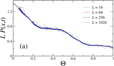
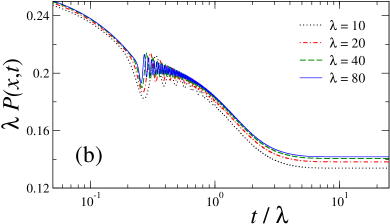
Figure 26: Dynamic scaling of the correlation function $P(x,t)={\rm Tr}\big{\{}\rho(t)\,\big{[}\hat{c}^{\dagger}_{j}\hat{c}^{\dagger}_{j+x}+\hat{c}_{j+x}\hat{c}_{j}\big{]}\big{\}}$, for a Kitaev quantum wire subject to dissipation induced by incoherent particle losses, for $\Gamma=uL=1$. Left panel $(a)$: test of dynamic FSS for a system in the presence of a quench in the Hamiltonian parameter, from $\Phi_{i}=0$ to $\Phi=2$. We fix $X=1/4$. The curves for different system sizes clearly approach a scaling function with increasing $L$, thus supporting the law in Eq. (310). Right panel $(b)$: test of dynamic thermodynamic-limit scaling for a static Hamiltonian, with $w_{i}=w=-1/\lambda$. We fix $x/\lambda=1$. The curves for different values of $\lambda$ approach a scaling function, following the scaling law (312). Adapted from Refs. [574, 821].

To characterize the dynamic properties of the evolution described by the Lindblad equation, we consider again the fixed-time correlations defined in Sec. 9.4, cf. Eqs. (232), evaluated on the mixed state $\rho(t)$. The expected dynamic scaling behavior is that reported in Eqs. (310), (312), and (313), with corresponding exponents $\varphi_{12}=1$ for the correlations $P$ and $C$, and $\varphi_{12}=2$ for $G$, as also mentioned in Sec. 9.4. The numerical results of Fig. 26 for the correlation function $P(x,t)$ in Eq. (232a) support: $(a)$ the dynamic FSS predicted by Eq. (310) and thus the fact that a nontrivial competition between critical coherence and dissipation can be only observed for $u\sim L^{-z}$, when $L$ increases in the dynamic FSS limit; $(b)$ the dynamic scaling in the thermodynamic limit, as reported in Eq. (312) . In particular, the curves converge to an asymptotic nontrivial behavior when increasing $L$ or $\lambda$. In this latter case, the long-time limit of such a curve for $\lambda\,P$ is different from zero, thus signaling the approach to a nontrivial stationary state. Therefore, in the case of homogenous dissipative schemes, the conjectured dynamic scaling, when keeping $\gamma=L^{z}u$ fixed, also describes the approach to the asymptotic stationary states. Indeed, for homogenous local dissipative mechanisms such as pumping or decay, $\Delta_{\cal L}$ scales as $\Delta_{\cal L}\sim 1/L$ when keeping $\gamma=Lu$ fixed, analogously to the critical gap $\Delta_{L}\sim 1/L$ at the CQT of the Kitaev wire. Therefore, the dynamic scaling can follow the whole dynamic process from $t=0$ to the asymptotic stationary states.

The dissipative scaling scenario has been numerically challenged [673] also within the quantum Ising chain (6) at its CQT, using the longitudinal field $h$ as driving Hamiltonian parameter, and local Lindblad operators $\hat{L}_{x}^{\pm}=\hat{\sigma}_{x}^{\pm}=\tfrac{1}{2}\big{[}\hat{\sigma}_{x}^{(1)}\pm i\hat{\sigma}_{x}^{(2)}\big{]}$. The computations of the dissipative dynamics are definitely harder for this problem, thus limiting them to much smaller systems, up to size $L\approx 10$.  Nevertheless, the obtained results are sufficient to support the dynamic scaling theory outlined in this section.

At this stage, we point out that notable differences emerge when the dissipative interactions with the environment are only localized at the boundary of a system at a CQT [834]. In particular the quantum evolution of fermionic Kitaev wires in the presence of dissipative (loss and pumping) boundaries, arising from protocols analogous to those considered in the presence of bulk dissipation, show two different dynamic regimes. There is an early-time regime for times $t\sim L$, where the competition between coherent and incoherent drivings develops a dynamic FSS analogous to that applying to bulk dissipations, but the boundary dissipative parameter (decay rate) does not apparently require to be tuned to zero. Then, there is a large-time regime for $t\sim L^{3}$, whose dynamic scaling describes the late quantum evolution leading to the $t\to\infty$ stationary states. The large time scales $t\sim L^{3}$ are essentially related to the fastest decay of the Lindbladian gap $\Delta_{\cal L}\sim L^{-3}$, which characterize several quantum spin chains and fermionic wires with boundary dissipations [822, 823, 819, 820].

13.5 Dissipative dynamics at first-order quantum transitions

The study of the effects of dissipative perturbations at QTs has been extended to FOQTs, where, analogously to what happens at CQTs, it is possible to recover a regime in which a nontrivial dynamic scaling behavior is developed [673]. This occurs when the dissipation parameter $u$ (globally controlling the decay rate of the dissipation within the master Lindblad equation) scales as the energy difference $\Delta$ of the lowest levels of the Hamiltonian of the many-body system, i.e., $u\sim\Delta$. However, unlike CQTs where $\Delta$ is power-law suppressed, at FOQTs the energy difference $\Delta$ is exponentially suppressed with increasing the system size (provided the BC do not favor any particular phase [55, 649]).

13.5.1 Quantum Ising models with local dissipators

Dissipative effects at FOQTs were studied within the paradigmatic 1$d$ Ising chain with PBC, along its FOQT line [673], thus with an exponentially suppressed energy difference of the two lowest levels, cf. Eq. (19b). The same quench protocol described in Sec. 13.1 has been considered, starting from the ground state of the Hamiltonian $\hat{H}_{\rm Is}(g<g_{c},h_{i})$, which is then subject to the time evolution ruled by Eq. (302), where $\hat{H}=\hat{H}_{\rm Is}(g<g_{c},h)$ and ${\mathbb{D}}[\rho]$ is the one reported in Eq. (316) with

$$\hat{L}_{x}=\hat{L}_{x}^{\pm}=\hat{\sigma}_{x}^{\pm}=\tfrac{1}{2}\big{[}\hat{\sigma}_{x}^{(1)}\pm i\hat{\sigma}_{x}^{(2)}\big{]}\,,$$ (318)

corresponding to mechanisms of incoherent raising ($+$) or lowering ($-$) for each spin of the chain. The out-of-equilibrium evolution, for $t>0$, can be monitored by measuring certain fixed-time observables, such as the longitudinal magnetization $M(t)$ of Eq. (174), evaluated on the the density matrix $\rho(t)$ of the system at time $t$, or by considering fixed-time spin correlations.

13.5.2 Dissipative dynamic scaling

As discussed in Sec. 13.3, at CQTs the dissipator ${\mathbb{D}}[\rho]$ typically drives the system to a noncritical steady state, even when the Hamiltonian parameters are close to those leading to a QT. However, one may identify a regime where the dissipation is sufficiently small to compete with the coherent evolution driven by the critical Hamiltonian, leading to potentially novel dynamic behaviors. At such low-dissipation regime, a dynamic scaling framework can be observed after appropriately rescaling the global dissipation parameter $u$, cf. Eq. (302a), introducing the corresponding scaling variable $\Gamma=u/\Delta(L)$. Within FOQTs, an analogous scaling scenario can be put forward, by extending the dynamic FSS of closed systems (Sec. 10), adding a further dependence on the scaling variable $\Gamma$ [574, 821]. For example, the dynamic scaling equation (235) for the magnetization is expected to change into

$$M(t;L,h_{i},h,u)\approx{\cal M}(\Theta,\Phi_{i},\Phi,\Gamma)\,,\qquad\Gamma={u\over\Delta(L)}\,,$$ (319)

where the scaling variables $\Theta$, $\Phi_{i}$ and $\Phi$, are defined in Eqs. (234) and (95).

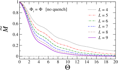
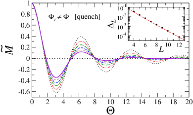
Figure 27: Time behavior of the longitudinal magnetization for a quantum Ising ring close to the FOQT, with $g=0.5$, in the presence of homogeneous dissipation described by local Lindblad operators $\hat{L}^{-}_{x}$. In particular, the figure shows the rescaled quantity $\widetilde{M}\equiv M(t;L,h_{i},h,u)/M(0;L,h_{i},h,u)$ versus the rescaled time $\Theta$, for different values of the system size $L$ (see legend). We fix the scaling variables $\Phi_{i}=1$ and $\Gamma=0.1$. The left panel is for $\Phi=\Phi_{i}$ (i.e., without quenching the Hamiltonian parameter $h$), while the right panel is for $\Phi=0$. The inset of the right panel shows the energy gap $\Delta_{L}$ as a function of $L$: black circles are the results obtained from the numerics, while the dashed red line denotes the estimate in Eq. (19b). Adapted from Ref. [673].

The numerical results reported in Fig. 27 for the time evolution of the longitudinal magnetization $M(t)$ support the above nontrivial dynamic scaling behavior [673]. The scaling law (319) has been checked by varying the Hamiltonian and the dissipation parameters of the protocol with increasing size $L$, so that the scaling variables $\Phi_{i}$, $\Phi$, and $\Gamma$ are kept fixed. For any nonzero value of the dissipation variable $\Gamma$, the longitudinal magnetization appears to asymptotically vanish in the large-time limit, although with different qualitative trends.

We mention that the dynamic behavior under global dissipators (right drawing of Fig. 25), given by

$${\mathbb{D}}[\rho]=\hat{L}\rho\hat{L}^{\dagger}-\tfrac{1}{2}\big{(}\rho\,\hat{L}^{\dagger}\hat{L}+\hat{L}^{\dagger}\hat{L}\rho\big{)}\,,\qquad\hat{L}^{\pm}\equiv\hat{\Sigma}^{\pm}\,,\qquad\hat{\Sigma}^{\pm}\equiv{1\over L}\sum_{x}\hat{\sigma}_{x}^{\pm}\,,$$ (320)

turns out to be well described by a single-spin model in the presence of a corresponding dissipator, showing that the system behaves rigidly, as already observed in other dynamic problems at FOQTs.

The arguments leading to the above scaling scenario at FOQTs are quite general. Analogous phenomena are expected to develop in any homogeneous $d$-dimensional many-body system at a FOQT, whose Markovian interactions with the bath can be described by local or extended dissipators within a Lindblad equation (302).

The dynamic scaling behavior turns out to become apparent already for relatively small systems, such as chains with $L\lesssim 10$. This makes such dynamic scaling phenomena relevant even from an experimental point of view, where the technical difficulties in manipulating and controlling such systems can be probably faced with up-to-date quantum simulation platforms.

13.6 Dissipation from the coupling with oscillator baths

One may consider an alternative mechanism leading to dissipation, in which the environment is effectively described by an infinite set of harmonic oscillators [843, 844]. For example, in the case of a spin system, such as the quantum Ising model (6), one may homogeneously couple each spin with an infinite number of quantum oscillators, through the coupling Hamiltonian term

$$\hat{H}_{{\rm Is-O}}=\sum_{\bm{x}}\hat{\sigma}^{(1)}_{\bm{x}}\sum_{k}\lambda_{k}\,(\hat{b}_{{\bm{x}},k}^{\dagger}+\hat{b}_{{\bm{x}},k})\,,$$ (321)

where $\hat{b}_{{\bm{x}},k}^{(\dagger)}$ are annihilation (creation) operators associated with the oscillators, whose Hamiltonian reads

$$\hat{H}_{{\rm O}}=\sum_{\bm{x}}\hat{H}_{{\rm O}{\bm{x}}}\,,\qquad\hat{H}_{{\rm O}{\bm{x}}}=\sum_{k}\omega_{k}\,\hat{b}_{{\bm{x}},k}^{\dagger}\hat{b}_{{\bm{x}},k}^{\phantom{\dagger}}\,.$$ (322)

The dissipation arising from these couplings is essentially determined by the spectral distribution of the oscillators coupled to the spin located at the site ${\bm{x}}$, and in particular on their power-law spectral density,

$$J(\omega)=\pi\sum_{k}\lambda_{k}\,\delta(\omega-\omega_{k})={\pi\over 2}\alpha\,\omega_{c}^{1-s}\,\omega^{s}\,,\qquad{\rm for}\;\;\omega<\omega_{c}\,,$$ (323)

and vanishing for $\omega>\omega_{c}$, therefore $\omega_{c}$ plays the role of high-energy cutoff, and $\alpha$ is a dimensionless measure of the dissipation strength. The value of the exponent $s$ determines the qualitative features of the dissipation. The experimentally important Ohmic dissipation, described by the case $s=1$, limits the super-Ohmic region $s>1$ where the bath effects are assumed to be weak.

These dissipative mechanisms have been investigated by several studies, in particular for the Ohmic case, showing that they can drive QTs. In particular, by exploiting the quantum-to-classical mapping into a statistical model with a further imaginary-time dimension, and integrating out the bath degrees of freedom, one obtains an effective action with long-range interactions along the imaginary time. The simplest models given by dissipative two-state (Ising) systems can be mapped into a classical $1d$ Ising model with long-range interactions decaying as $1/r^{1+s}$. As shown by several studies (see, e.g., Refs. [844, 845, 846, 847, 848]), they develop a phase transition between localized and delocalized phases. New classes of phase transitions (generally different from those of the isolated systems) are also observed for many-body systems [849, 850, 851, 852, 853], such as the quantum Ising chain coupled to oscillator baths as in Eqs. (321) and (322), which can be mapped into a classical $2d$ system with long-range interactions along one of the directions.

We finally note that the dissipative mechanisms based on the coupling with infinite sets of oscillators tend to suppress the critical behavior at the QTs of isolated systems, analogously to the dissipative perturbations described within the Lindblad framework. The effects of the above oscillator baths at the QTs of isolated systems may be treated within dynamic scaling frameworks analogous to those outlined in this section. However, unlike the Lindblad frameworks, such mechanisms may themselves lead to QTs belonging to different universality classes, corresponding to statistical systems with long-range interactions. On the other hand, the nature of the phase transition that dissipative Lindblad mechanisms may stabilize in the stationary large-time limit is substantially different, more similar to the finite-temperature transitions [791]. For this reason, one does not expect phase transitions driven by Lindblad dissipative mechanisms within $1d$ quantum models with short-range interactions.

14 Dissipation in the out-of-equilibrium Kibble-Zurek dynamics

As already discussed in Sec. 9, slow passages through QTs allow to probe some universal features of quantum fluctuations. In this respect, we recall the KZ problem [693, 695, 539, 543], related to the amount of final defects, after slow (quasi-adiabatic) passages through CQTs, from the disordered to the ordered phase. Since dissipative mechanisms are expected to give rise to relevant perturbations at the quantum criticality of closed systems, such as the temperature, they do not generally preserve the universal dynamic properties of QTs. Therefore, the open nature of quantum systems leads to a departure from the dynamic KZ scaling behavior predicted for the isolated case [854, 855, 856, 857, 858, 859, 841, 860, 861, 862, 863, 864, 650, 865, 866]. In particular, it has been observed that slow quenches in open systems, or subject to noisy controls, may generate an overabundance of defects, when approaching the adiabatic limit in KZ protocols [718]. Nonetheless, taking into account the role of dissipation is crucial to understand the outcomes of experimental results for quantum annealing protocols (see Sec. 9.5), as recently shown during the simulation of quasi-adiabatic passages across the CQT of quantum Ising systems, in the presence of a dissipative dynamics modeled by the coupling to an Ohmic bath of harmonic oscillators [867, 868].

Due to the general relevance of the perturbations associated with dissipative mechanisms, slower protocols favor the dissipation effects, in that they give them more time to act. Therefore, unlike closed systems, the dynamic behaviors arising from slow changes of the Hamiltonian parameters, across their critical values, do not anymore develop universal critical features controlled by the QT of the closed system. One thus expects that only an appropriate tuning of the dissipation strength may originate a nontrivial interplay with the critical unitary dynamics. This issue is best discussed within a dynamic scaling framework, based on the extension of the scaling theory for KZ dynamics in closed systems (Sec. 9), to allow for the dissipative perturbations. Open dissipative systems may still present a universal regime controlled by the universality class of the QT of the closed system, provided the system-environment interaction strength is suitably tuned analogously to the quench dynamics in the presence of dissipative perturbations, that we have already discussed in the previous section 13.

14.1 Dynamic Kibble-Zurek scaling for open quantum systems

The KZ protocol in the presence of dissipative mechanisms is analogous to that considered for closed systems, and discussed in Sec. 9.1, with the only addition of dissipation during the whole dynamics. Namely, we assume again that the many-body Hamiltonian depends on a parameter $w(t)$, which is linearly modulated in time as in Eq. (214), and can be written as

$$\hat{H}(t)=\hat{H}_{c}+w(t)\hat{H}_{p}\,,\qquad w(t)=t/t_{s}\,.$$ (324)

The many-body system is supposed to be initialized in the ground state of $\hat{H}(t_{i})$ at $t_{i}<0$ corresponding to $w_{i}=w(t_{i})<0$. Subsequently, at time $t>t_{i}$, it evolves according to the Lindblad master equation (302), with the above time-dependent Hamiltonian $\hat{H}(t)$ and with a fixed dissipation strength.

On these grounds, a dynamic KZ scaling theory allowing for the dissipative perturbation can be obtained by extending the one for closed systems outlined in Sec. 9.3. For this purpose, one should also allow for a further dependence of the various scaling functions on a new scaling variable associated with the dissipation parameter $u$ in the dynamic scaling relations (46). In practice, this can be taken as a power law $b^{z}\,u$, where the dynamic exponent $z$ ensures the substantial balance (competition) with the critical coherent driving.

14.1.1 Dissipative scaling in the thermodynamic limit

To obtain the dissipative KZ scaling in the thermodynamic limit, one may again start from the homogeneous laws in terms of the arbitrary length scale $b$, fix it as in Eq. (218), and then take the limit $L/b\to\infty$. The net result are scaling equations analogous to those reported in Sec. 9.3.1, with a further dependence on the scaling variable

$$\Gamma_{s}=t_{s}^{\kappa}\,u\,,\qquad\kappa={z\over y_{w}+z}\,,$$ (325)

associated with the dissipation strength $u$. Thus, we obtain

$$G_{12}(t,t_{s},{\bm{x}};w_{i},u)\approx\lambda^{-\varphi_{12}}\,{\cal G}_{\infty}({\bm{x}}/\lambda,\Omega_{t},\lambda^{y_{w}}w_{i},\Gamma_{s})\,.$$ (326)

This is expected to provide the asymptotic behavior in the $t_{s}\to\infty$ limit, while keeping the scaling variables fixed, including $\Gamma_{s}$. For $\Gamma_{s}\to 0$, we must recover the scaling laws of the closed systems subject to the unitary evolution only. More importantly, the above scaling law tells us that the dissipation effects are expected to be negligible when $u\ll t_{s}^{-\kappa}$, and dominant when $u\gg t_{s}^{-\kappa}$.

Note that, like for closed systems, the large-$t_{s}$ limit of KZ protocols starting from finite and fixed $w_{i}<0$ corresponds to the limit $\lambda^{y_{w}}w_{i}\to-\infty$. Indeed, the dissipation with coupling strength $u\sim\lambda^{-z}$ is not expected to play any relevant role at finite $w_{i}<0$, where the gap is $\Delta=O(1)$, while it should compete with the unitary evolution only very close to $w=0$ where $u\sim\Delta\sim\lambda^{-z}$. Therefore, under such conditions, the scaling behavior simplifies to

$$G_{12}(t,t_{s},{\bm{x}};w_{i},u)\approx\lambda^{-\varphi_{12}}\,{\cal G}_{\infty}({\bm{x}}/\lambda,\Omega_{t},\Gamma_{s})\,,$$ (327)

becoming independent on the initial $w_{i}$. The dissipative KZ scaling limit also implies that the scaling law associated with the number of defects, cf. Eq. (226), should be replaced with [650]

$$\rho_{\rm def}\approx\lambda^{-d}\,\widetilde{\cal R}_{\rm def}(\Omega_{t},\Gamma_{s})=t_{s}^{-{d\over y_{\mu}+z}}\,{\cal R}_{\rm def}(\Omega_{t},\Gamma_{s})\,,$$ (328)

where the dependence on the dissipative coupling $u$ enters the scaling function ${\cal R}_{\rm def}$ through the scaling variable $\Gamma_{s}$. Of course, for $u=0$ (thus $\Gamma_{s}=0$) one recovers the scaling law for closed systems [cf. Eq. (226)].

14.1.2 Dissipative scaling in the finite-size scaling limit

Analogously to the dynamics of closed systems, it is possible to derive scaling laws in the FSS limit, by fixing $b=L$ in the homogeneous scaling laws, such as Eqs. (46) with the further dependence on $b^{z}\,u$. The resulting scaling ansatz for two-point correlation functions turns out to be analogous to that of closed systems, i.e., Eq. (228), with in addition a dependence on the scaling variable $\Gamma=L^{z}\,u$ related to the dissipative strength,

$$G_{12}(t,t_{s},{\bm{x}};L,w_{i},u)=\big{\langle}\hat{O}_{1}({\bm{x}}_{1})\,\hat{O}_{2}({\bm{x}}_{2})\big{\rangle}_{t}\approx L^{-\varphi_{12}}\,{\cal G}_{12}(\Omega_{t},{\bm{X}},\Upsilon,\Omega_{t_{i}},\Gamma)\,.$$ (329)

Moreover, assuming again that the quantum phase for $w_{i}<0$ is gapped, with $\Delta\sim\xi^{-z}$, and the ground-state length scale $\xi$ diverges only at the critical point $w=0$, KZ protocols associated with any finite initial $w_{i}<0$ develop the same dynamic FSS independently of their actual values, corresponding to $\Omega_{t_{i}}\to-\infty$, and therefore its dependence can be dropped when considering a dynamic KZ scaling at fixed $w_{i}$.

14.2 Results for the Kitaev quantum wire subject to dissipation

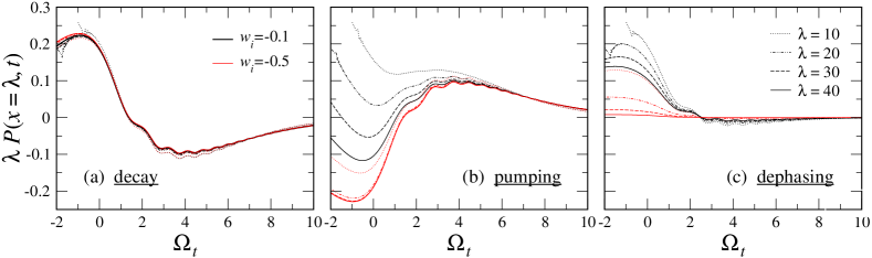
Figure 28: Rescaled correlations $\lambda\,P(x,t)$ at fixed initial $w_{i}$, for the dissipative Kitaev quantum wire in the thermodynamic limit, as a function of the scaling variable $\Omega_{t}$. Here we fix $x/\lambda=1$ and $\Gamma_{s}=0.5$. Each panel refers to a specific type of dissipation mechanism [see Eq. (317)]: decay $(a)$, pumping $(b)$, and dephasing $(c)$. The color code refers to $w_{i}=-0.1$ (black) and $w_{i}=-0.5$ (red). Different line styles are for various values of $\lambda$, from $10$ to $40$ (see legend). Adapted from Ref. [650].

Accurate numerical checks of the dissipative KZ scaling behaviors have been reported for the Kitaev quantum wire in the presence of local dissipative mechanisms, such as those already considered in Sec. 13.4, related to local pumping, decay, and dephasing dissipative mechanisms [cf. Eqs. (317)]. As already mentioned, this model is amenable to a direct solvability for systems with $O(10^{3})$ sites, thus representing the ideal playground for open quantum lattice problems, given the remarkable difficulty to simulate the dynamics of many-body quantum systems coupled to an external bath. To monitor the dynamics arising from the dissipative KZ protocol, we consider again the fixed-time correlation functions defined in Eq. (232). They are expected to show the dissipative KZ scaling reported in Eq. (327) in the thermodynamic limit, and in Eq. (329) in the FSS limit, similarly to the dissipative scaling in quench protocols (see Sec. 13.4).

Fig. 28 shows some numerical outcomes for the correlation function $P(x,t)$ in the thermodynamic limit, cf. Eq. (232a), for a fixed value of $\Gamma_{s}$, two different values of $w_{i}=\mu_{i}-\mu_{c}$, and various values of $\lambda$. The dephasing seems to be the most disruptive dissipation mechanism. However in all cases we observe that, with increasing $\lambda$, they approach the same asymptotic behavior, irrespective of the choice of $w_{i}$; for the incoherent decay, this appears to be much faster than for the other kinds of dissipation. It can be also shown that the convergence to the asymptotic behavior with $\lambda$, for given $\Omega_{t}$, is power law as expected. Results for the same correlation function at finite size are provided in Fig. 29, supporting the dynamic FSS put forward in Eq. (329). The various panels, for different initial values of $w_{i}$, show convergence with $L$ to a scaling function, which appears to be the same in all cases: the magnified bottom panels at large $\Omega_{t}$ unveil how discrepancies in the temporal behavior, starting from different $w_{i}$, get suppressed in the large-$L$ limit.

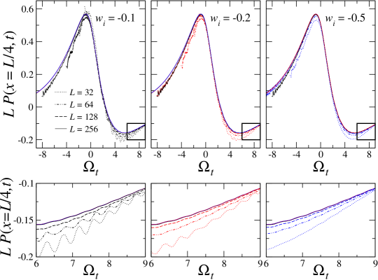
Figure 29: The rescaled correlation $L\,P(x,t)$, with $x/L=1/4$, as a function of $\Omega_{t}$, fixing the initial Hamiltonian parameter $w_{i}=-0.1$ (left panels, black curves), $-0.2$ (central panels, red curves), and $-0.5$ (right panels, blue curves). Different line styles stand for various $L$ (see legend). The lower panels show magnifications of the upper ones, for $6\leq\Omega_{t}\leq 9$. We fix $\Upsilon=0.1$ and $\Gamma=1$, with dissipation given by incoherent decay. The three continuous curves, corresponding to the largest size $L=256$ and different $w_{i}$, are plotted in each of the six panels for reference, and cannot be distinguished on the scale of the plots reported. Adapted from Ref. [650].

We emphasize that, to obtain the correct asymptotic KZ scaling behavior, it is crucial to allow for the dissipation to be suitably rescaled in the large-$t_{s}$ limit. That is, the parameter $u$ entering the dissipator in the Lindblad master equation (302a) must be scaled as $u\sim t_{s}^{-\kappa}$, meaning that the scaling variable $\Gamma_{s}=u\,t_{s}^{\kappa}$ has to be kept fixed. In contrast, if the dissipation strength $u$ is not changed with $t_{s}$, no dynamic scaling can be observed using KZ-like protocols [650].

15 Measurement-induced dynamics at quantum transitions

In general, while the unitary evolution enhances the entanglement, measurements of observables disentangle degrees of freedom and thus tend to decrease quantum correlations, similarly to decoherence. A projective quantum measurement is physically realized when the interaction with a macroscopic object makes a quantum mechanical system rapidly collapse into an eigenstate of a specific operator, and the resulting time evolution appears to be a non-unitary projection. Such process is referred to as a projective measurement [756, 869]. When the system is projected into an eigenstate of a local operator, the corresponding local degree of freedom is disentangled from the rest of the system. Moreover, if projective measurements are performed frequently, the quantum state gets localized in the Hilbert space near a trivial product state, leading to the quantum Zeno effect [870, 871]. In strongly correlated systems, QTs give rise to a peculiar dynamic regime where long-range correlations set in; the impact of projective quantum measurements on the decay rate of quantum correlations should be thus substantially affected by the emerging critical dynamics.

To address the interplay of unitary and projective dynamics in experimentally viable many-body systems at QTs, such as quantum spin networks, one may consider dynamic problems arising from protocols combining the unitary Hamiltonian and local measurement drivings (for a cartoon, see Fig. 30). In such conditions, different regimes emerge, depending on the measurement schemes and their parameters. If every site were measured during each projective step, the system would be continually reset to a tensor product state. More intriguing scenarios should hold when local measurements are spatially dilute.

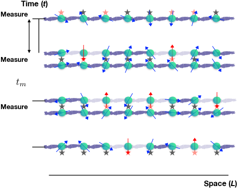
Figure 30: Sketch of a quantum-measurement protocol: A quantum spin system, initially frozen in its ground state at quantum criticality ($t=0$), is perturbed with local projective measurements (stars) occurring after every time interval $t_{m}$, with a homogeneous probability $p$ per site. In between two measurement steps, the system evolves unitarily, according to its Hamiltonian. Red stars denote the occurrence of a measurement on a given site (for the sake of clarity, in the figure we consider $\hat{\sigma}^{(3)}$-type measures: spins colored in red are projected along the $z$-axis). From Ref. [872].

Most of the work done in this context focuses on the investigation of entanglement transitions genuinely driven by local measurements, either in random circuits [30, 32, 33, 31, 873, 874, 875, 876, 877, 878, 879], in the BH model [880, 881], in quantum spin systems [882, 883, 884, 885, 886, 887], or in free-fermionic chains [888, 889, 890, 891, 892], and on measurement-induced state preparation [893]. In noninteracting models, continuous local measurements were shown to largely suppress entanglement. Here we review a substantially different dynamic problem, related to the effects of local random measurements on the quantum critical dynamics of many-body systems, i.e., when a QT is driven by the Hamiltonian parameters [872].

Different regimes arise from the interplay between unitary and projective dynamics in critical systems. One of them is dominated by local random measurements, for example for any finite probability $p$ of making the local measurement. In contrast, for sufficiently small $p$ values (decreasing as a sufficiently large power of the inverse diverging length scale $\xi$), the measurements are irrelevant. These two regimes turn out to be separated by dynamic conditions leading to peculiar dynamic scaling behaviors, controlled by the universality class of the QT. For a $d$-dimensional critical system, scaling arguments lead to the exact power law

$$p\sim\xi^{-(z+d)}\,.$$ (330)

Therefore, local measurements generally suppress quantum correlations, even in the dynamic scaling limit, with scaling laws that are qualitatively different when being far from criticality. The corresponding time scale at a QT is indeed expected to behave as

$$\tau_{m}\sim\xi^{z}\sim p^{-\kappa}\,,\qquad\kappa={z\over z+d}<1\,,$$ (331)

to be compared with the noncritical case $\tau_{m}\sim p^{-1}$.

15.1 Measurement protocols for quantum Ising models

We discuss quantum lattice spin systems, assuming that only one relevant parameter $w$ of the Hamiltonian $\hat{H}(w)$ (with RG dimension $y_{w}>0$) can deviate from the QCP, located at $w_{c}=0$. For example, we may consider the paradigmatic $d$-dimensional quantum Ising Hamiltonian (6) of size $L^{d}$ with PBC, at its CQT point driven by the relevant parameters $r=g-g_{c}$ and $h$, which we may identify with the driving parameter $w$. The following measurement protocol can be adopted:

• The system is initialized, at $t=0$, in the ground state $|\Psi_{0}(w)\rangle$ close to criticality, thus $|w|\ll 1$.

• Random local projective measurements are performed at every time interval $t_{m}$, so that each site has a (homogeneous) probability $p$ to be measured. For the quantum Ising model, one may consider local measurements of the spin components, along transverse [$\hat{\sigma}_{\bm{x}}^{(3)}$] or longitudinal [$\hat{\sigma}_{\bm{x}}^{(1)}$] directions.

• The updated many-body wave function is obtained by projecting onto the spin state at site ${\bm{x}}$ corresponding to the measured value of the spin component, and normalizing it.

• In between two measurement steps, the system evolves according to the unitary operator $e^{-i\hat{H}(w)t}$.

If $p\to 1$, each spin gets measured every $t_{m}$, and the effects of projections are expected to dominate over those of the unitary evolution. In contrast, for $p$ sufficiently small, the time evolution may result unaffected by measurements. In between these two regimes, there is a competing unitary vs. projective dynamics, characterized by controllable dynamic scaling behaviors associated with the universality class of the QT.

The evolution along the above protocol can be monitored by fixed-time averages of observables, as the longitudinal magnetization $M(t)$ and the susceptibility $\chi(t)$,

$$m(t)=L^{-d}\sum_{\bm{x}}\big{\langle}\hat{\sigma}_{\bm{x}}^{(1)}\big{\rangle}_{t}\,,\qquad\chi(t)=L^{-d}\sum_{{\bm{x}},{\bm{y}}}\big{\langle}\hat{\sigma}_{\bm{x}}^{(1)}\,\hat{\sigma}_{\bm{y}}^{(1)}\big{\rangle}_{t}\,,$$ (332)

averaging over the trajectories. The time scale $\tau_{m}$ of the suppression of quantum correlations can be estimated from the halving time of the ratio

$$R_{\chi}(t)\equiv\frac{\chi(t)-1}{\chi(t=0)-1}\,,\qquad R_{\chi}(t)\in[0,1]\,,$$ (333)

which is expected to go from one ($t=0$) to zero ($t\to\infty$). Indeed note that, since projective measurements generally suppress quantum correlations, $\lim_{t\to\infty}\chi(t)=1$, corresponding to an uncorrelated state.

15.2 Phenomenological dynamic scaling theory

We now present a phenomenological scaling theory for the out-of-equilibrium dynamics arising from random local projective measurements during the evolution of a many-body system at a QT. The starting point is a homogeneous scaling law allowing for the measurement process, and in particular for the parameters associated with measurement protocol. We write

$$O(t;L,w;t_{m},p)\approx b^{-y_{o}}\,{\cal O}(b^{-z}t,b^{-1}L,b^{y_{w}}w,b^{\zeta}t_{m},b^{\varepsilon}p)\,,$$ (334)

where $\zeta$ and $\varepsilon$ are appropriate exponents associated with the measurement process. The above scaling equation is supposed to provide the power-law asymptotic behavior in the large-$b$ limit, neglecting further dependences on other parameters, which are supposed to be suppressed (and thus irrelevant) in such limit.

The arbitrariness of the scale parameter $b$ in Eq. (334) can be fixed by setting $b=\lambda\equiv|w|^{-1/y_{w}}$, where $\lambda\sim\xi$ is the length scale of critical modes. The scaling variable associated with the time interval $t_{m}$ should be given by the product $\Delta\,t_{m}$, where $\Delta^{-1}\sim\lambda^{z}$ is the time scale of the critical models (this implies $\zeta=-z$). Keeping $t_{m}$ fixed in the large-$\lambda$ limit, the dependence on $t_{m}$ disappears asymptotically, originating only $O(\lambda^{-z})$ scaling corrections. Moreover, noticing that $p$ is effectively a probability per unit of time and space, a reasonable guess would be its correct scaling to compete with the critical modes, that is $p\sim\lambda^{-z-d}$, thus

$$\varepsilon=z+d\,.$$ (335)

This leads to the dynamic scaling equation

$$O(t;w;t_{m},p)\approx\lambda^{-y_{o}}\,{\cal O}(\lambda^{-z}t,\lambda^{\varepsilon}p)\,.$$ (336)

The value of $\varepsilon$ in Eq. (335) is crucial, since it provides the condition that separates the measurement-irrelevant regime $p=o(\lambda^{-\varepsilon})$ from the measurement-dominant regime $\lambda^{\varepsilon}\,p\to\infty$. Since $p\sim\lambda^{-\varepsilon}$ and $t\sim\lambda^{z}$, the dynamic scaling ansatz predicts that the time scale $\tau_{m}$ associated with the suppression of quantum correlations behaves as $\tau_{m}\sim p^{-\kappa}$ with $\kappa=z/\varepsilon<1$.

The above scaling theory holds in the thermodynamic limit $L/\lambda\to\infty$, that is expected to be well defined for any $w\neq 0$, for which $\lambda$ is finite. Nonetheless, for most practical purposes, both experimental and numerical, one typically has to face with systems of finite length. Such situations can be framed in the FSS framework, where the scale parameter in Eq. (334) is set to $b=L$. Fixing again $t_{m}$, one obtains the scaling law

$$O(t;L,w;t_{m},p)\approx L^{-y_{o}}\,{\cal O}(\Theta,\Phi,L^{\varepsilon}p)\,,$$ (337)

so that the proper dynamic FSS behavior is obtained in the thermodynamic limit, taking the scaling variables $\Theta=L^{-z}\,t$, $\Phi=L^{y_{w}}\,w$, and $L^{\varepsilon}\,p$ fixed.

Analogous scaling ansatze for more general observables, as fixed-time correlation functions, are obtainable with the same arguments and assumptions. They can be extended to include an initial quench of the Hamiltonian parameter $w_{i}\to w$ [by adding a further dependence on $b^{y_{w}}\,w_{i}$ in Eq. (334), corresponding to the further scaling variable $\Phi_{i}=L^{y_{w}}\,w_{i}$ in Eq. (337)], to consider finite-temperature initial Gibbs states [by adding a dependence on $b^{z}\,T$ in Eq. (334), corresponding to the further scaling variable $\Xi=T/\Delta(L)$ in Eq. (337)], and also allowing for weak dissipation. Note also that the scaling arguments do not depend on the type of local measurement, therefore they are expected to be generally independent of them, to some extent.

15.3 Numerical evidence in favor of the dynamic scaling theory

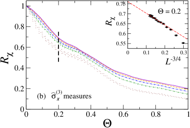
Figure 31: Time behavior of $R_{\chi}$ in the quantum Ising chain at criticality, for various sizes. Random measurements are either along the longitudinal [panel $(a)$] or the transverse [panel $(b)$] direction. Here $t_{m}=0.1$, while $p=1/L^{2}$ has been fixed according to the guess (335). The two insets display data for specific values of $\Theta$ (dashed lines in the main frames), showing that the convergence to the asymptotic behavior is compatible with a $O(L^{-3/4})$ approach (dashed red lines). Adapted from Ref. [872].

The above phenomenological scaling theory has been checked on the quantum Ising chain. The dynamic FSS laws for the magnetization and its susceptibility follow Eq. (337), in which the parameter $w$ corresponds to either $r=g-g_{c}$ or $h$ in Eq. (113). In particular, for $r=h=0$, one obtains $m(t)=0$ by symmetry, and

$$R_{\chi}(t;L;t_{m},p)\approx{\cal R}_{\chi}(L^{-z}t,L^{\varepsilon}p)\,.$$ (338)

Results for a system at its QCP, with random local longitudinal and transverse spin measurements, are shown in Fig. 31. Data for $R_{\chi}$ versus $\Theta=L^{-z}\,t$ nicely agree with Eq. (338), and corrections to the scaling are consistent with a power-law suppression as $L^{-3/4}$ approach, as expected [650]. Analogous scaling results are obtained in the small-$t_{m}$ limit, and also for the magnetization at $h\neq 0$, keeping $\Phi=L^{y_{h}}\,h$ constant.

The above scaling behaviors can be compared with situations far from QTs, for example in the quantum disordered phase $g>g_{c}$ of quantum Ising models, where the length scale $\xi$ of quantum correlations and the gap $\Delta$ remain finite with increasing $L$. Away from criticality, the characteristic time $\tau_{m}$ of the measurements scales as $\tau_{m}\sim p^{-1}$, unlike the critical behavior, where $\tau_{m}\sim p^{-\kappa}$ with $\kappa=z/\varepsilon<1$. The smaller power $\kappa$ at criticality (i.e., faster decay rate) can be explained by the fact that the relevant probability ($p_{r}$) driving the measurement process is the one to perform a local measurement within the critical volume $\xi^{d}$, therefore $p_{r}=\xi^{d}\,p$. The time rate thus behaves as $\tau_{m}\sim p_{r}^{-1}$, similarly to the noncritical case, where $\xi=O(1)$. Of course, this implies that the critical conditions significantly speed up the decoherence process arising from the local quantum measurements [650].

16 Outlook and Applications

We have presented a series of issues concerning the equilibrium and out-of-equilibrium behavior of quantum many-body systems in proximity of quantum phase transitions. The competition between quantum fluctuations, either at equilibrium or along the out-of-equilibrium unitary dynamics, and decohering effects induced by the temperature, the environment, or quantum measurements, probably represents the most intricate dynamic regime where complex many-body phenomena may appear. Notwithstanding the apparent difficulty in treating this kind of situations, a universal behavior forcefully emerges if the system stays close to a zero-temperature quantum transition, of both continuous and first-order types.

We wrote this review with the purpose to collect and elucidate the scaling behaviors that may naturally emerge in the thermodynamic and the FSS limits, providing a unified framework where both continuous and first-order quantum transitions can be quantitatively investigated with a satisfactory accuracy. The emerging dynamic scaling scenario is quite general, in the sense that it is expected to hold for generic quantum transitions in any spatial dimension. Although, at the time of writing this review, most of the out-of-equilibrium dynamic scaling arguments, and related predictions, have been explicitly verified by computations within quantum $1d$ Ising-like systems or Kitaev fermionic wires, the general ideas should apply to other quantum many-body systems, as well. We mention, for example, fermionic or bosonic Hubbard-like models, with any geometry, and also in the presence of different dissipative schemes, such as in a non-Markovian setting. Moreover, one could consider the presence of defects, with various possible geometries. It would be thus tempting to investigate and carefully verify the dynamic scaling behavior in other situations, where novel features may arise.

16.1 Experimental feasibility

In view of the impressive experimental advances that have been achieved in this new millennium era in quantum simulation and quantum computing [894, 526], we hope this review will stimulate further progress and foster the investigations in a field that, according to us, can be legitimately considered as one of the great challenges of contemporary physics. In fact, we hope that the FSS predictions described are amenable to a direct verification in the laboratory, by means of small-size quantum simulators operating on a limited amount of quantum objects (of the order of ten, or few tens).

A number of remarkable experiments already demonstrated their capability to faithfully reproduce and control the dynamics of many-body quantum systems, such as Ising- or Hubbard-like models. Some platforms are best suited for specific conditions, however the cross-fertilization between the various available possibilities is likely to provide us further precious insight in this fascinating field of research in physics. Among the others, we mention the following platforms:

• Ultracold atoms in artificial optical lattices [166, 525, 895]. Optical lattices are formed by the interference pattern of counter-propagating laser beams in different directions, which create a regular pattern mimicking the crystalline structure of a solid. Atoms feel the periodic potential landscape induced by lasers via the Stark shift. This kind of setup is extremely clean and controllable, such that the dynamics of isolated quantum many-body systems can be studied, keeping coherence for a significant amount of time. In practice, the Hamiltonian parameters can be tuned close to quantum transition points and also easily varied in time. Single-site addressability is not a severe concern [896, 222, 897]. For all these reasons, cold atoms are one of the best options to study quantum many-body systems at equilibrium and in nondissipative out-of-equilibrium conditions (see, e.g., Refs. [221, 898, 545, 899, 548, 549, 900, 901, 578]). Dissipation can be included by suitable bath engineering and/or using Rydberg atoms [902], which also enable to tune the range of interactions [903].

• Trapped ions [904, 905]. It is possible to form ion crystals by balancing the Coulomb repulsion between ions and the trap confinement force, allowing them to be accurately controlled and manipulated, as well as to produce long-range and tunable interactions. They already proved their great potential in the simulation of Ising-like spin systems, where each spin is represented by suitable internal energy levels of a single ion [748, 747, 751, 749, 584, 750, 752]. Ions can be addressed and measured locally, at the level of a fully-programmable quantum simulator [754]. The range of interactions and the addition of disorder can be adjusted in a controllable way [582, 906].

• Nuclear and electronic spins in solid-state structures [907, 908, 909, 910]. They demonstrated their versatility in reproducing the physics of non-equilibrium many-body quantum systems and of quantum criticality, using different platforms. We mention:

  • Nuclear magnetic resonance, which permits to manipulate a dozen of interacting spins, showing long coherence times and a high degree of controllability [773, 911, 912].

  • Nitrogen vacancy centers in diamond [909, 913].

  • Arrays of semiconductor quantum dots [914, 915].

• Coupled quantum electrodynamics (QED). Using hybrid platforms, one can induce strong effective interaction between photons [916, 27, 917, 29, 28]. Collective light-matter excitations in these systems are called polaritons. Dissipation is naturally present in the photonic components of the polaritons, therefore it is possible to simulate archetypal lattice models under driven nonequilibrium conditions. Different experimental platforms have been taken into account:

  • Photonic crystals or fibers. The confinement of photons in optical systems, as fibers or arrays of microcavities filled with atoms, enables the generation of large, tunable nonlinearities. It is thus possible to simulate strongly interacting quantum many-body systems as Hubbard-like models or spin chains [918, 919, 920].

  • Semiconductor microcavities. The confined photons are strongly coupled to electronic excitations, leading to the creation of exciton polaritons. So far, most of the experimental results have been obtained in the mean-field regime, originating from the collective behavior of a large number of polaritons, described via a single wave function. Macroscopic quantum coherence has been observed in nonequilibrium Bose-Einstein condensation [921] or polariton superfluidity [922].

  • Circuit QED [923]. Superconducting circuits are among the most promising platforms to engineer quantum simulators and quantum computers, being easily scalable and highly flexible in the nanofabrication. Photonic modes are realized from a co-planar transmission line or an LC circuit acting as a microwave cavity; nonlinearities can be induced through Josephson junctions. Several aspects of the many-body quantum physics, including phase transitions, quantum criticality, Kibble-Zurek physics, many-body localization, have been addressed (see, e.g., Refs. [924, 925, 818, 926, 927]).

  • Coupled optomechanical cavities [928, 929]. Inside each cavity, a localized mechanical mode interacts with a laser-driven cavity mode via radiation pressure; neighboring cavities are effectively coupled through photon and phonon hopping.

References

- Sachdev [2011] S. Sachdev, Quantum phase transitions, 2 ed., Cambridge University Press, Cambridge, 2011. doi:10.1017/CBO9780511973765.
- Sondhi et al. [1997] S. L. Sondhi, S. M. Girvin, J. P. Carini, D. Shahar, Continuous quantum phase transitions, Rev. Mod. Phys. 69 (1997) 315. URL: http://arxiv.org/abs/cond-mat/9609279. doi:10.1103/RevModPhys.69.315.
- Vojta [2019] M. Vojta, Disorder in quantum many-body systems, Annu. Rev. Condens. Matter Phys. 10 (2019) 233. URL: http://arxiv.org/abs/1806.05611. doi:10.1146/annurev-conmatphys-031218-013433.
- Dziarmaga [2010] J. Dziarmaga, Dynamics of a quantum phase transition and relaxation to a steady state, Adv. Phys. 59 (2010) 1063. URL: http://arxiv.org/abs/0912.4034. doi:10.1080/00018732.2010.514702.
- Polkovnikov et al. [2011] A. Polkovnikov, K. Sengupta, A. Silva, M. Vengalattore, Colloquium: Nonequilibrium dynamics of closed interacting quantum systems, Rev. Mod. Phys. 83 (2011) 863. URL: http://arxiv.org/abs/1007.5331. doi:10.1103/RevModPhys.83.863.
- Eisert et al. [2015] J. Eisert, M. Friesdorf, C. Gogolin, Quantum many-body systems out of equilibrium, Nat. Phys. 11 (2015) 124. URL: http://arxiv.org/abs/1408.5148. doi:10.1038/nphys3215.
- Gogolin and Eisert [2016] C. Gogolin, J. Eisert, Equilibration, thermalisation, and the emergence of statistical mechanics in closed quantum systems, Rep. Prog. Phys. 79 (2016) 056001. URL: http://arxiv.org/abs/1503.07538. doi:10.1088/0034-4885/79/5/056001.
- D’Alessio et al. [2016] L. D’Alessio, Y. Kafri, A. Polkovnikov, M. Rigol, From quantum chaos and eigenstate thermalization to statistical mechanics and thermodynamics, Adv. Phys. 65 (2016) 239. URL: http://arxiv.org/abs/1509.06411. doi:10.1080/00018732.2016.1198134.
- Mori et al. [2018] T. Mori, T. N. Ikeda, E. Kaminishi, M. Ueda, Thermalization and prethermalization in isolated quantum systems: A theoretical overview, J. Phys. B: At. Mol. Opt. Phys. 51 (2018) 112001. URL: http://arxiv.org/abs/1712.08790. doi:10.1088/1361-6455/aabcdf.
- Nandkishore and Huse [2015] R. Nandkishore, D. A. Huse, Many body localization and thermalization in quantum statistical mechanics, Annu. Rev. Condens. Matter Phys. 6 (2015) 15. URL: http://arxiv.org/abs/1404.0686. doi:10.1146/annurev-conmatphys-031214-014726.
- Altman and Vosk [2015] E. Altman, R. Vosk, Universal dynamics and renormalization in many-body-localized systems, Annu. Rev. Condens. Matter Phys. 6 (2015) 383. URL: http://arxiv.org/abs/1408.2834. doi:10.1146/annurev-conmatphys-031214-014701.
- Vasseur and Moore [2016] R. Vasseur, J. E. Moore, Nonequilibrium quantum dynamics and transport: From integrability to many-body localization, J. Stat. Mech. (2016) 064010. URL: http://arxiv.org/abs/1603.06618. doi:10.1088/1742-5468/2016/06/064010.
- Abanin and Papić [2017] D. A. Abanin, Z. Papić, Recent progress in many‐body localization, Ann. Phys. 529 (2017) 1700169. URL: http://arxiv.org/abs/1705.09103. doi:10.1002/andp.201700169.
- Alet and Laflorencie [2018] F. Alet, N. Laflorencie, Many-body localization: An introduction and selected topics, C. R. Phys. 19 (2018) 498. URL: http://arxiv.org/abs/1711.03145. doi:10.1016/j.crhy.2018.03.003.
- Abanin et al. [2019] D. A. Abanin, E. Altman, I. Bloch, M. Serbyn, Colloquium: Many-body localization, thermalization, and entanglement, Rev. Mod. Phys. 91 (2019) 021001. URL: http://arxiv.org/abs/1804.11065. doi:10.1103/RevModPhys.91.021001.
- Essler and Fagotti [2016] F. H. L. Essler, M. Fagotti, Quench dynamics and relaxation in isolated integrable quantum spin chains, J. Stat. Mech. (2016) 064002. URL: http://arxiv.org/abs/1603.06452. doi:10.1088/1742-5468/2016/06/064002.
- Vidmar and Rigol [2016] L. Vidmar, M. Rigol, Generalized Gibbs ensemble in integrable lattice models, J. Stat. Mech. (2016) 064007. URL: http://arxiv.org/abs/1604.03990. doi:10.1088/1742-5468/2016/06/064007.
- Ilievski et al. [2016] E. Ilievski, M. Medenjak, T. Prosen, L. Zadnik, Quasilocal charges in integrable lattice systems, J. Stat. Mech. (2016) 064008. URL: http://arxiv.org/abs/1603.00440. doi:10.1088/1742-5468/2016/06/064008.
- Langen et al. [2016] T. Langen, T. Gasenzer, J. Schmiedmayer, Prethermalization and universal dynamics in near-integrable quantum systems, J. Stat. Mech. (2016) 064009. URL: http://arxiv.org/abs/1603.09385. doi:10.1088/1742-5468/2016/06/064009.
- Zvyagin [2016] A. A. Zvyagin, Dynamical quantum phase transitions (Review Article), Low. Temp. Phys. 42 (2016) 971. URL: http://arxiv.org/abs/1701.08851. doi:10.1063/1.4969869.
- Heyl [2018] M. Heyl, Dynamical quantum phase transitions: A review, Rep. Prog. Phys. 81 (2018) 054001. URL: http://arxiv.org/abs/1709.07461. doi:10.1088/1361-6633/aaaf9a.
- Grifoni and Hänggi [1998] M. Grifoni, P. Hänggi, Driven quantum tunneling, Phys. Rep. 304 (1998) 229. doi:10.1016/S0370-1573(98)00022-2.
- Bukov et al. [2015] M. Bukov, L. D’Alessio, A. Polkovnikov, Universal high-frequency behavior of periodically driven systems: From dynamical stabilization to Floquet engineering, Adv. Phys. 64 (2015) 139. URL: http://arxiv.org/abs/1407.4803. doi:10.1080/00018732.2015.1055918.
- Holthaus [2016] M. Holthaus, Floquet engineering with quasienergy bands of periodically driven optical lattices, J. Phys. B: At. Mol. Opt. Phys. 49 (2016) 013001. URL: http://arxiv.org/abs/1510.09042. doi:10.1088/0953-4075/49/1/013001.
- Sacha and Zakrzewski [2018] K. Sacha, J. Zakrzewski, Time crystals: A review, Rep. Prog. Phys. 81 (2018) 016401. URL: http://arxiv.org/abs/1704.03735. doi:10.1088/1361-6633/aa8b38.
- Else et al. [2020] D. V. Else, C. Monroe, C. Nayak, N. Y. Yao, Discrete time crystals, Annu. Rev. Condens. Matter Phys. 11 (2020) 467. URL: http://arxiv.org/abs/1905.13232. doi:10.1146/annurev-conmatphys-031119-050658.
- Carusotto and Ciuti [2013] I. Carusotto, C. Ciuti, Quantum fluids of light, Rev. Mod. Phys. 85 (2013) 299. URL: http://arxiv.org/abs/1205.6500. doi:10.1103/RevModPhys.85.299.
- Noh and Angelakis [2017] C. Noh, D. G. Angelakis, Quantum simulations and many-body physics with light, Rep. Prog. Phys. 80 (2017) 016401. URL: http://arxiv.org/abs/1604.04433. doi:10.1088/0034-4885/80/1/016401.
- Hartmann [2016] M. J. Hartmann, Quantum simulation with interacting photons, J. Opt. 18 (2016) 104005. URL: http://arxiv.org/abs/1605.00383. doi:10.1088/2040-8978/18/10/104005.
- Li et al. [2018] Y. Li, X. Chen, M. P. A. Fisher, Quantum Zeno effect and the many-body entanglement transition, Phys. Rev. B 98 (2018) 205136. URL: http://arxiv.org/abs/1808.06134. doi:10.1103/PhysRevB.98.205136.
- Li et al. [2019] Y. Li, X. Chen, M. P. A. Fisher, Measurement-driven entanglement transition in hybrid quantum circuits, Phys. Rev. B 100 (2019) 134306. URL: http://arxiv.org/abs/1901.08092. doi:10.1103/PhysRevB.100.134306.
- Chan et al. [2019] A. Chan, R. M. Nandkishore, M. Pretko, G. Smith, Unitary-projective entanglement dynamics, Phys. Rev. B 99 (2019) 224307. URL: http://arxiv.org/abs/1808.05949. doi:10.1103/PhysRevB.99.224307.
- Skinner et al. [2019] B. Skinner, J. Ruhman, A. Nahum, Measurement-induced phase transitions in the dynamics of entanglement, Phys. Rev. X 9 (2019) 031009. URL: http://arxiv.org/abs/1808.05953. doi:10.1103/PhysRevX.9.031009.
- Vojta [2003] M. Vojta, Quantum phase transitions, Rep. Prog. Phys. 66 (2003) 2069. URL: http://arxiv.org/abs/cond-mat/0309604. doi:10.1088/0034-4885/66/12/R01.
- Belitz et al. [2005] D. Belitz, T. R. Kirkpatrick, T. Vojta, How generic scale invariance influences quantum and classical phase transitions, Rev. Mod. Phys. 77 (2005) 579. URL: http://arxiv.org/abs/cond-mat/0403182. doi:10.1103/RevModPhys.77.579.
- Sachdev and Keimer [2011] S. Sachdev, B. Keimer, Quantum criticality, Phys. Today 64 (2011) 29. URL: http://arxiv.org/abs/1102.4628. doi:10.1063/1.3554314.
- Dutta et al. [2015] A. Dutta, G. Aeppli, B. K. Chakrabarti, U. Divakaran, T. F. Rosenbaum, D. Sen, Quantum phase transitions in transverse field spin models: From statistical physics to quantum information, Cambridge University Press, Cambridge, 2015. doi:10.1017/CBO9781107706057.
- Wilson and Kogut [1974] K. G. Wilson, J. Kogut, The renormalization group and the expansion, Phys. Rep. 12 (1974) 75. doi:10.1016/0370-1573(74)90023-4.
- Fisher [1974] M. E. Fisher, The renormalization group in the theory of critical behavior, Rev. Mod. Phys. 46 (1974) 597. doi:10.1103/RevModPhys.46.597, [Erratum: ibid. 47 (1975), 543].
- S.-k. Ma [2001] S.-k. Ma, Modern theory of critical phenomena, Routledge, New York, 2001. doi:10.4324/9780429498886.
- Brézin et al. [1976] E. Brézin, J. C. L. Guillou, J. Zinn-Justin, Field theoretical approach to critical phenomena, in: C. Domb, M. S. Green (Eds.), Phase transitions and critical phenomena, volume 6, Academic Press, London, 1976, p. 125.
- Wegner [1976] F. J. Wegner, The critical state, general aspects, in: C. Domb, J. L. Lebowitz (Eds.), Phase transitions and critical phenomena, volume 6, Academic Press, London, 1976, p. 7.
- Patashinskii and Pokrovskii [1979] A. Z. Patashinskii, V. L. Pokrovskii, Fluctuation theory of phase transitions, Pergamon Press, Oxford, 1979. doi:10.1002/bbpc.19800840723.
- Wilson [1983] K. G. Wilson, The renormalization group and critical phenomena, Rev. Mod. Phys. 55 (1983) 583. doi:10.1103/RevModPhys.55.583.
- Itzykson and Drouffe [1989] C. Itzykson, J.-M. Drouffe, Statistical field theory: Volume 1. From Brownian motion to renormalization and lattice gauge theory, Cambridge University Press, Cambridge, 1989. doi:10.1017/CBO9780511622779.
- Zinn-Justin [2002] J. Zinn-Justin, Quantum field theory and critical phenomena, 4 ed., Clarendon Press, Oxford, 2002. doi:10.1093/acprof:oso/9780198509233.001.0001.
- Cardy [1996] J. Cardy, Scaling and renormalization in statistical physics, Cambridge University Press, Cambridge, 1996. doi:10.1017/CBO9781316036440.
- Fisher [1998] M. E. Fisher, Renormalization group theory: Its basis and formulation in statistical physics, Rev. Mod. Phys. 70 (1998) 653. doi:10.1103/RevModPhys.70.653.
- Pelissetto and Vicari [2002] A. Pelissetto, E. Vicari, Critical phenomena and renormalization-group theory, Phys. Rep. 368 (2002) 549. URL: http://arxiv.org/abs/cond-mat/0012164. doi:10.1016/S0370-1573(02)00219-3.
- Amit and V. Martin-Mayor [2005] D. J. Amit, V. Martin-Mayor, Field theory, the renormalization group, and critical phenomena: Graphs to computers, 3 ed., World Scientific, Singapore, 2005. doi:10.1142/5715.
- Berezinskii [1971] V. L. Berezinskii, Destruction of long-range order in one-dimensional and two-dimensional systems having a continuous symmetry group I. Classical systems, Sov. Phys. JETP 32 (1971) 493.
- Berezinskii [1972] V. L. Berezinskii, Destruction of long-range order in one-dimensional and two-dimensional systems possessing a continuous symmetry group. II. Quantum systems, Sov. Phys. JETP 34 (1972) 610.
- Kosterlitz and Thouless [1973] J. M. Kosterlitz, D. J. Thouless, Ordering, metastability and phase transitions in two-dimensional systems, J. Phys. C: Solid State Phys. 6 (1973) 1181. doi:10.1088/0022-3719/6/7/010.
- Kosterlitz [1974] J. M. Kosterlitz, The critical properties of the two-dimensional xy model, J. Phys. C: Solid State Phys. 7 (1974) 1046. doi:10.1088/0022-3719/7/6/005.
- Campostrini et al. [2014] M. Campostrini, J. Nespolo, A. Pelissetto, E. Vicari, Finite-size scaling at first-order quantum transitions, Phys. Rev. Lett. 113 (2014) 070402. URL: http://arxiv.org/abs/1405.6823. doi:10.1103/PhysRevLett.113.070402.
- Campostrini et al. [2015a] M. Campostrini, A. Pelissetto, E. Vicari, Quantum transitions driven by one-bond defects in quantum Ising rings, Phys. Rev. E 91 (2015a) 042123. URL: http://arxiv.org/abs/1501.03265. doi:10.1103/PhysRevE.91.042123.
- Campostrini et al. [2015b] M. Campostrini, A. Pelissetto, E. Vicari, Quantum Ising chains with boundary fields, J. Stat. Mech. (2015b) P11015. URL: http://arxiv.org/abs/1507.08391. doi:10.1088/1742-5468/2015/11/P11015.
- Landau [1937a] L. Landau, On the theory of phase transitions. I., Phys. Z. Sowjetunion 11 (1937a) 26.
- Landau [1937b] L. Landau, On the theory of phase transitions. II., Phys. Z. Sowjetunion 11 (1937b) 545.
- Wilson [1971a] K. G. Wilson, Renormalization group and critical phenomena. I. Renormalization group and the Kadanoff scaling picture, Phys. Rev. B 4 (1971a) 3174. doi:10.1103/PhysRevB.4.3174.
- Wilson [1971b] K. G. Wilson, Renormalization group and critical phenomena. II. Phase-space cell analysis of critical behavior, Phys. Rev. B 4 (1971b) 3184. doi:10.1103/PhysRevB.4.3184.
- Vicari and Zinn-Justin [2006] E. Vicari, J. Zinn-Justin, Fixed point stability and decay of correlations, New J. Phys. 8 (2006) 321. URL: http://arxiv.org/abs/cond-mat/0611353. doi:10.1088/1367-2630/8/12/321.
- Vicari [2008] E. Vicari, Critical phenomena and renormalization-group flow of multi-parameter field theories, PoS Lattice 2007 (2008) 023. URL: http://arxiv.org/abs/0709.1014. doi:10.22323/1.042.0023.
- Aharony [1976] A. Aharony, Dependence of universal critical behavior on symmetry and range of interaction, in: C. Domb, J. L. Lebowitz (Eds.), Phase transitions and critical phenomena, volume 6, Academic Press, London, 1976, p. 357.
- Carmona et al. [2000] J. M. Carmona, A. Pelissetto, E. Vicari, -component Ginzburg-Landau Hamiltonian with cubic anisotropy: A six-loop study, Phys. Rev. B 61 (2000) 15136. URL: http://arxiv.org/abs/cond-mat/9912115. doi:10.1103/PhysRevB.61.15136.
- Harris [1974] A. B. Harris, Effect of random defects on the critical behaviour of Ising models, J. Phys. C: Solid State Phys. 7 (1974) 1671. doi:10.1088/0022-3719/7/9/009.
- Pelissetto and Vicari [2000] A. Pelissetto, E. Vicari, Randomly dilute spin models: A six-loop field-theoretic study, Phys. Rev. B 62 (2000) 6393. URL: http://arxiv.org/abs/cond-mat/0002402. doi:10.1103/PhysRevB.62.6393.
- Kawamura [1998] H. Kawamura, Universality of phase transitions of frustrated antiferromagnets, J. Phys.: Condens. Matter 10 (1998) 4707. URL: http://arxiv.org/abs/cond-mat/9805134. doi:10.1088/0953-8984/10/22/004.
- Pelissetto et al. [2001] A. Pelissetto, P. Rossi, E. Vicari, Critical behavior of frustrated spin models with noncollinear order, Phys. Rev. B 63 (2001) 140414(R). URL: http://arxiv.org/abs/cond-mat/0007389. doi:10.1103/PhysRevB.63.140414.
- Calabrese et al. [2002] P. Calabrese, P. Parruccini, A. I. Sokolov, Chiral phase transitions: Focus driven critical behavior in systems with planar and vector ordering, Phys. Rev. B 66 (2002) 180403(R). URL: http://arxiv.org/abs/cond-mat/0205046. doi:10.1103/PhysRevB.66.180403.
- Delamotte et al. [2004] B. Delamotte, D. Mouhanna, M. Tissier, Nonperturbative renormalization-group approach to frustrated magnets, Phys. Rev. B 69 (2004) 134413. URL: http://arxiv.org/abs/cond-mat/0309101. doi:10.1103/PhysRevB.69.134413.
- Calabrese et al. [2004] P. Calabrese, P. Parruccini, A. Pelissetto, E. Vicari, Critical behavior of symmetric models, Phys. Rev. B 70 (2004) 174439. URL: http://arxiv.org/abs/cond-mat/0405667. doi:10.1103/PhysRevB.70.174439.
- Zhang et al. [2002] Y. Zhang, E. Demler, S. Sachdev, Competing orders in a magnetic field: Spin and charge order in the cuprate superconductors, Phys. Rev. B 66 (2002) 094501. URL: http://arxiv.org/abs/cond-mat/0112343. doi:10.1103/PhysRevB.66.094501.
- Sachdev [2003] S. Sachdev, Colloquium: Order and quantum phase transitions in the cuprate superconductors, Rev. Mod. Phys. 75 (2003) 913. URL: http://arxiv.org/abs/cond-mat/0211005. doi:10.1103/RevModPhys.75.913.
- M. De Prato et al. [2004] M. De Prato, A. Pelissetto, E. Vicari, Normal-to-planar superfluid transition in 3He, Phys. Rev B 70 (2004) 214519. URL: http://arxiv.org/abs/cond-mat/0312362. doi:10.1103/PhysRevB.70.214519.
- M. De Prato et al. [2006] M. De Prato, A. Pelissetto, E. Vicari, Spin-density-wave order in cuprates, Phys. Rev. B 74 (2006) 144507. URL: http://arxiv.org/abs/cond-mat/0601404. doi:10.1103/PhysRevB.74.144507.
- Pelissetto et al. [2008] A. Pelissetto, S. Sachdev, E. Vicari, Nodal quasiparticles and the onset of spin-density-wave order in cuprate superconductors, Phys. Rev. Lett. 101 (2008) 027005. URL: http://arxiv.org/abs/0802.0199. doi:10.1103/PhysRevLett.101.027005.
- Kim et al. [2008] E.-A. Kim, M. J. Lawler, P. Oreto, S. Sachdev, E. Fradkin, S. A. Kivelson, Theory of the nodal nematic quantum phase transition in superconductors, Phys. Rev. B 77 (2008) 184514. URL: http://arxiv.org/abs/0705.4099. doi:10.1103/PhysRevB.77.184514.
- Fisher and Nelson [1974] M. E. Fisher, D. R. Nelson, Spin flop, supersolids, and bicritical and tetracritical points, Phys. Rev. Lett. 32 (1974) 1350. doi:10.1103/PhysRevLett.32.1350.
- Nelson et al. [1974] D. R. Nelson, J. M. Kosterlitz, M. E. Fisher, Renormalization-group analysis of bicritical and tetracritical points, Phys. Rev. Lett. 33 (1974) 813. doi:10.1103/PhysRevLett.33.813.
- Kosterlitz et al. [1976] J. M. Kosterlitz, D. R. Nelson, M. E. Fisher, Bicritical and tetracritical points in anisotropic antiferromagnetic systems, Phys. Rev. B 13 (1976) 412. doi:10.1103/PhysRevB.13.412.
- Calabrese et al. [2003] P. Calabrese, A. Pelissetto, E. Vicari, Multicritical phenomena in -symmetric theories, Phys. Rev. B 67 (2003) 054505. URL: http://arxiv.org/abs/cond-mat/0209580. doi:10.1103/PhysRevB.67.054505.
- Pisarski and Wilczek [1984] R. D. Pisarski, F. Wilczek, Remarks on the chiral phase transition in chromodynamics, Phys. Rev. D 29 (1984) 338(R). doi:10.1103/PhysRevD.29.338.
- Butti et al. [2003] A. Butti, A. Pelissetto, E. Vicari, On the nature of the finite-temperature transition in QCD, J. High. Energy Phys. 08 (2003) 029. URL: http://arxiv.org/abs/hep-ph/0307036. doi:10.1088/1126-6708/2003/08/029.
- Pelissetto and Vicari [2013] A. Pelissetto, E. Vicari, Relevance of the axial anomaly at the finite-temperature chiral transition in QCD, Phys. Rev. D 88 (2013) 105018. URL: http://arxiv.org/abs/1309.5446. doi:10.1103/PhysRevD.88.105018.
- Campostrini et al. [2014] M. Campostrini, A. Pelissetto, E. Vicari, Finite-size scaling at quantum transitions, Phys. Rev. B 89 (2014) 094516. URL: http://arxiv.org/abs/1401.0788. doi:10.1103/PhysRevB.89.094516.
- Xu [2012] C. Xu, Unconventional quantum critical points, Int. J. Mod. Phys. B 26 (2012) 1230007. URL: http://arxiv.org/abs/1202.6065. doi:10.1142/S0217979212300071.
- Sachdev [2019] S. Sachdev, Topological order, emergent gauge fields, and Fermi surface reconstruction, Rep. Prog. Phys. 82 (2019) 014001. URL: http://arxiv.org/abs/1801.01125. doi:10.1088/1361-6633/aae110.
- Belitz et al. [2002] D. Belitz, T. R. Kirkpatrick, T. Vojta, Local versus nonlocal order-parameter field theories for quantum phase transitions, Phys. Rev. B 65 (2002) 165112. URL: http://arxiv.org/abs/cond-mat/0109547. doi:10.1103/PhysRevB.65.165112.
- Bi et al. [2020] Z. Bi, E. Lake, T. Senthil, Landau ordering phase transitions beyond the Landau paradigm, Phys. Rev. Research 2 (2020) 023031. URL: http://arxiv.org/abs/1910.12856. doi:10.1103/PhysRevResearch.2.023031.
- Hasan and Kane [2010] M. Z. Hasan, C. L. Kane, Colloquium: Topological insulators, Rev. Mod. Phys. 82 (2010) 3045. URL: http://arxiv.org/abs/1002.3895. doi:10.1103/RevModPhys.82.3045.
- Qi and Zhang [2011] X.-L. Qi, S.-C. Zhang, Topological insulators and superconductors, Rev. Mod. Phys. 83 (2011) 1057. URL: http://arxiv.org/abs/1008.2026. doi:10.1103/RevModPhys.83.1057.
- Wen [2007] X.-G. Wen, Quantum field theory of many-body systems: From the origin of sound to an origin of light and electrons, Oxford University Press, Oxford, 2007. doi:10.1093/acprof:oso/9780199227259.001.0001.
- Fradkin [2013] E. Fradkin, Field theories of condensed matter physics, 2 ed., Cambridge University Press, Cambridge, 2013. doi:10.1017/CBO9781139015509.
- Zeng et al. [2019] B. Zeng, X. Chen, D.-L. Zhou, X.-G. Wen, Quantum information meets quantum matter: From quantum entanglement to topological phases of many-body systems, Springer-Verlag, New York, 2019. doi:10.1007/978-1-4939-9084-9.
- Gulden et al. [2016] T. Gulden, M. Janas, Y. Wang, A. Kamenev, Universal finite-size scaling around topological quantum phase transitions, Phys. Rev. Lett. 116 (2016) 026402. URL: http://arxiv.org/abs/1508.03646. doi:10.1103/PhysRevLett.116.026402.
- Read and Sachdev [1990] N. Read, S. Sachdev, Spin-Peierls, valence-bond solid, and Néel ground states of low-dimensional quantum antiferromagnets, Phys. Rev. B 42 (1990) 4568. doi:10.1103/PhysRevB.42.4568.
- Senthil et al. [2004a] T. Senthil, L. Balents, S. Sachdev, A. Vishwanath, M. P. A. Fisher, Quantum criticality beyond the Landau-Ginzburg-Wilson paradigm, Phys. Rev. B 70 (2004a) 144407. URL: http://arxiv.org/abs/cond-mat/0312617. doi:10.1103/PhysRevB.70.144407.
- Senthil et al. [2004b] T. Senthil, A. Vishwanath, L. Balents, S. Sachdev, M. P. A. Fisher, Deconfined quantum critical points, Science 303 (2004b) 1490. URL: http://arxiv.org/abs/cond-mat/0311326. doi:10.1126/science.1091806.
- Huckestein [1995] B. Huckestein, Scaling theory of the integer quantum Hall effect, Rev. Mod. Phys. 67 (1995) 357. URL: http://arxiv.org/abs/cond-mat/9501106. doi:10.1103/RevModPhys.67.357.
- Hansson et al. [2017] T. H. Hansson, M. Hermanns, S. H. Simon, S. F. Viefers, Quantum Hall physics: Hierarchies and conformal field theory techniques, Rev. Mod. Phys. 89 (2017) 025005. URL: http://arxiv.org/abs/1601.01697. doi:10.1103/RevModPhys.89.025005.
- Giesbers et al. [2009] A. J. M. Giesbers, U. Zeitler, L. A. Ponomarenko, R. Yang, K. S. Novoselov, A. K. Geim, J. C. Maan, Scaling of the quantum Hall plateau-plateau transition in graphene, Phys. Rev. B 80 (2009) 241411(R). URL: http://arxiv.org/abs/0908.0461. doi:10.1103/PhysRevB.80.241411.
- Obuse et al. [2012] H. Obuse, I. A. Gruzberg, F. Evers, Finite-size effects and irrelevant corrections to scaling near the integer quantum Hall transition, Phys. Rev. Lett. 109 (2012) 206804. URL: http://arxiv.org/abs/1205.2763. doi:10.1103/PhysRevLett.109.206804.
- Wegner [1971] F. J. Wegner, Duality in generalized Ising models and phase transitions without local order parameters, J. Math. Phys. 12 (1971) 2259. doi:10.1063/1.1665530.
- Lieb et al. [1961] E. Lieb, T. Schultz, D. Mattis, Two soluble models of an antiferromagnetic chain, Ann. Phys. 16 (1961) 407. doi:10.1016/0003-4916(61)90115-4.
- Katsura [1962] S. Katsura, Statistical mechanics of the anisotropic linear Heisenberg model, Phys. Rev. 127 (1962) 1508. doi:10.1103/PhysRev.127.1508, [Erratum: ibid. 129 (1963), 2835].
- A. Yu. Kitaev [2001] A. Yu. Kitaev, Unpaired Majorana fermions in quantum wires, Phys. Usp. 44 (2001) 131. URL: http://arxiv.org/abs/cond-mat/0010440. doi:10.1070/1063-7869/44/10S/S29.
- Pfeuty [1970] P. Pfeuty, The one-dimensional Ising model with a transverse field, Ann. Phys. 57 (1970) 79. doi:10.1016/0003-4916(70)90270-8.
- Burkhardt and Guim [1985] T. W. Burkhardt, I. Guim, Finite-size scaling of the quantum Ising chain with periodic, free, and antiperiodic boundary conditions, J. Phys. A: Math. Gen. 18 (1985) L33. doi:10.1088/0305-4470/18/1/006.
- Fisher and Barber [1972] M. E. Fisher, M. N. Barber, Scaling theory for finite-size effects in the critical region, Phys. Rev. Lett. 28 (1972) 1516. doi:10.1103/PhysRevLett.28.1516.
- Barber [1983] M. N. Barber, Finite-size scaling, in: C. Domb, J. L. Lebowitz (Eds.), Phase transitions and critical phenomena, volume 8, Academic Press, London, 1983, p. 145.
- Privman [1990] V. Privman (Ed.), Finite size scaling and numerical simulation of statistical systems, World Scientific, Singapore, 1990. doi:10.1142/1011.
- Binder [1987] K. Binder, Theory of first-order phase transitions, Rep. Prog. Phys. 50 (1987) 783. doi:10.1088/0034-4885/50/7/001.
- Privman et al. [1991] V. Privman, P. C. Hohenberg, A. Aharony, Universal critical-point amplitude relations, in: C. Domb, J. L. Lebowitz (Eds.), Phase transitions and critical phenomena, volume 14, Academic Press, London, 1991, p. 1.
- Cardy [1988] J. Cardy, Finite-size scaling, Volume 2, 1 ed., North Holland, Amsterdam, 1988.
- Itzykson and Drouffe [1989] C. Itzykson, J.-M. Drouffe, Statistical field theory: Volume 2. Strong coupling, Monte Carlo methods, conformal field theory and random systems, Cambridge University Press, Cambridge, 1989. doi:10.1017/CBO9780511622786.
- P. Di Francesco et al. [1997] P. Di Francesco, P. Mathieu, D. Sénéchal, Conformal field theory, Springer-Verlag, New York, 1997. doi:10.1007/978-1-4612-2256-9.
- Henkel [1987] M. Henkel, Finite-size scaling and universality in the spectrum of the quantum ising chain. I. Periodic and antiperiodic boundary condition, J. Phys. A: Math. Gen. 20 (1987) 995. doi:10.1088/0305-4470/20/4/033.
- Reinicke [1987a] P. Reinicke, Finite-size scaling functions and conformal invariance, J. Phys. A: Math. Gen. 20 (1987a) 4501. doi:10.1088/0305-4470/20/13/048.
- Reinicke [1987b] P. Reinicke, Analytical and non-analytical corrections to finite-size scaling, J. Phys. A: Math. Gen. 20 (1987b) 5325. doi:10.1088/0305-4470/20/15/044.
- Calabrese et al. [2000] P. Calabrese, M. Caselle, A. Celi, A. Pelissetto, E. Vicari, Nonanalyticity of the Callan-Symanzik -function of two-dimensional O() models, J. Phys. A: Math. Gen. 33 (2000) 8155. URL: http://arxiv.org/abs/hep-th/0005254. doi:10.1088/0305-4470/33/46/301.
- Caselle et al. [2002] M. Caselle, M. Hasenbusch, A. Pelissetto, E. Vicari, Irrelevant operators in the two-dimensional Ising model, J. Phys. A: Math. Gen. 35 (2002) 4861. URL: http://arxiv.org/abs/cond-mat/0106372. doi:10.1088/0305-4470/35/23/305.
- Campostrini et al. [2002] M. Campostrini, A. Pelissetto, P. Rossi, E. Vicari, 25th-order high-temperature expansion results for three-dimensional Ising-like systems on the simple-cubic lattice, Phys. Rev. E 65 (2002) 066127. URL: http://arxiv.org/abs/cond-mat/0201180. doi:10.1103/PhysRevE.65.066127.
- Deng and Blöte [2003] Y. Deng, H. W. J. Blöte, Simultaneous analysis of several models in the three-dimensional Ising universality class, Phys. Rev. E 68 (2003) 036125. doi:10.1103/PhysRevE.68.036125.
- Hasenbusch [2010] M. Hasenbusch, Finite size scaling study of lattice models in the three-dimensional Ising universality class, Phys. Rev. B 82 (2010) 174433. URL: http://arxiv.org/abs/1004.4486. doi:10.1103/PhysRevB.82.174433.
- Guida and Zinn-Justin [1998] R. Guida, J. Zinn-Justin, Critical exponents of the -vector model, J. Phys. A: Math. Gen. 31 (1998) 8103. URL: http://arxiv.org/abs/cond-mat/9803240. doi:10.1088/0305-4470/31/40/006.
- Kompaniets and Panzer [2017] M. V. Kompaniets, E. Panzer, Minimally subtracted six-loop renormalization of O()-symmetric theory and critical exponents, Phys. Rev. D 96 (2017) 036016. URL: http://arxiv.org/abs/1705.06483. doi:10.1103/PhysRevD.96.036016.
- G. De Polsi et al. [2020] G. De Polsi, I. Balog, M. Tissier, N. Wschebor, Precision calculation of critical exponents in the O() universality classes with the nonperturbative renormalization group, Phys. Rev. E 101 (2020) 042113. URL: http://arxiv.org/abs/2001.07525. doi:10.1103/PhysRevE.101.042113.
- Kos et al. [2016] F. Kos, D. Poland, D. Simmons-Duffin, A. Vichi, Precision islands in the Ising and O() models, J. High Energy Phys. 08 (2016) 036. URL: http://arxiv.org/abs/1603.04436. doi:10.1007/JHEP08(2016)036.
- Hasenbusch [2001] M. Hasenbusch, Monte Carlo studies of the three-dimensional Ising model in equilibrium, Int. J. Mod. Phys. C 12 (2001) 911. doi:10.1142/S0129183101002383.
- Hasenbusch [1999] M. Hasenbusch, A Monte Carlo study of leading order scaling corrections of theory on a three-dimensional lattice, J. Phys. A: Math. Gen. 32 (1999) 4851. URL: http://arxiv.org/abs/hep-lat/9902026. doi:10.1088/0305-4470/32/26/304.
- Antonenko and Sokolov [1995] S. A. Antonenko, A. I. Sokolov, Critical exponents for a three-dimensional O()-symmetric model with , Phys. Rev. E 51 (1995) 1894. URL: http://arxiv.org/abs/hep-th/9803264. doi:10.1103/PhysRevE.51.1894.
- J. C. Le Guillou and Zinn-Justin [1977] J. C. Le Guillou, J. Zinn-Justin, Critical exponents for the -vector model in three dimensions from field theory, Phys. Rev. Lett. 39 (1977) 95. doi:10.1103/PhysRevLett.39.95.
- J. C. Le Guillou and Zinn-Justin [1980] J. C. Le Guillou, J. Zinn-Justin, Critical exponents from field theory, Phys. Rev. B 21 (1980) 3976. doi:10.1103/PhysRevB.21.3976.
- Baker et al. [1976] G. A. Baker, B. G. Nickel, M. S. Green, D. I. Meiron, Ising-model critical indices in three dimensions from the Callan-Symanzik equation, Phys. Rev. Lett. 36 (1976) 1351. doi:10.1103/PhysRevLett.36.1351.
- Parisi [1980] G. Parisi, Field-theoretic approach to second-order phase transitions in two- and three-dimensional systems, J. Stat. Phys. 23 (1980) 49. doi:10.1007/BF01014429.
- Chetyrkin et al. [1983] K. G. Chetyrkin, S. G. Gorishny, S. A. Larin, F. V. Tkachov, Five-loop renormalization group calculations in the theory, Phys. Lett. B 132 (1983) 351. doi:10.1016/0370-2693(83)90324-6.
- Wilson and Fisher [1972] K. G. Wilson, M. E. Fisher, Critical exponents in 3.99 dimensions, Phys. Rev. Lett. 28 (1972) 240. doi:10.1103/PhysRevLett.28.240.
- G. ’t Hooft and Veltman [1972] G. ’t Hooft, M. Veltman, Regularization and renormalization of gauge fields, Nucl. Phys. B 44 (1972) 189. doi:10.1016/0550-3213(72)90279-9.
- Poland et al. [2019] D. Poland, S. Rychkov, A. Vichi, The conformal bootstrap: Theory, numerical techniques, and applications, Rev. Mod. Phys. 91 (2019) 015002. URL: http://arxiv.org/abs/1805.04405. doi:10.1103/RevModPhys.91.015002.
- Zhang et al. [2009] J. Zhang, F. M. Cucchietti, C. M. Chandrashekar, M. Laforest, C. A. Ryan, M. Ditty, A. Hubbard, J. K. Gamble, R. Laflamme, Direct observation of quantum criticality in Ising spin chains, Phys. Rev. A 79 (2009) 012305. URL: http://arxiv.org/abs/0808.1536. doi:10.1103/PhysRevA.79.012305.
- Coldea et al. [2010] R. Coldea, D. A. Tennant, E. M. Wheeler, E. Wawrzynska, D. Prabhakaran, M. Telling, K. Habicht, P. Smeibidl, K. Kiefer, Quantum criticality in an Ising chain: Experimental evidence for emergent symmetry, Science 327 (2010) 177. URL: http://arxiv.org/abs/1103.3694. doi:10.1126/science.1180085.
- Morris et al. [2014] C. M. Morris, R. Valdés Aguilar, A. Ghosh, S. M. Koohpayeh, J. Krizan, R. J. Cava, O. Tchernyshyov, T. M. McQueen, N. P. Armitage, Hierarchy of bound states in the one-dimensional ferromagnetic Ising chain investigated by high-resolution time-domain terahertz spectroscopy, Phys. Rev. Lett. 112 (2014) 137403. URL: http://arxiv.org/abs/1312.4514. doi:10.1103/PhysRevLett.112.137403.
- Kinross et al. [2014] A. W. Kinross, M. Fu, T. J. Munsie, H. A. Dabkowska, G. M. Luke, S. Sachdev, T. Imai, Evolution of quantum fluctuations near the quantum critical point of the transverse field Ising chain system , Phys. Rev. X 4 (2014) 031008. URL: http://arxiv.org/abs/1401.6917. doi:10.1103/PhysRevX.4.031008.
- Liang et al. [2015] T. Liang, S. M. Koohpayeh, J. W. Krizan, T. M. McQueen, R. J. Cava, N. P. Ong, Heat capacity peak at the quantum critical point of the transverse Ising magnet , Nat. Commun. 6 (2015) 7611. URL: http://arxiv.org/abs/1405.4551. doi:10.1038/ncomms8611.
- Bach et al. [2019] C. T. Bach, N. T. Nguyen, G. H. Bach, Thermodynamic properties of ferroics described by the transverse Ising model and their applications for , J. Magn. Magn. Mater. 483 (2019) 136. URL: http://arxiv.org/abs/1809.07985. doi:10.1016/j.jmmm.2019.03.093.
- Privman and Fisher [1983] V. Privman, M. E. Fisher, Finite-size effects at first-order transitions, J. Stat. Phys. 33 (1983) 385. doi:10.1007/BF01009803.
- Cabrera and Jullien [1987] G. G. Cabrera, R. Jullien, Role of boundary conditions in the finite-size Ising model, Phys. Rev. B 35 (1987) 7062. doi:10.1103/PhysRevB.35.7062.
- Alicea [2012] J. Alicea, New directions in the pursuit of Majorana fermions in solid state systems, Rep. Prog. Phys. 75 (2012) 076501. URL: http://arxiv.org/abs/1202.1293. doi:10.1088/0034-4885/75/7/076501.
- Laumann et al. [2012] C. R. Laumann, R. Moessner, A. Scardicchio, S. L. Sondhi, Quantum adiabatic algorithm and scaling of gaps at first-order quantum phase transitions, Phys. Rev. Lett. 109 (2012) 030502. URL: http://arxiv.org/abs/1202.3646. doi:10.1103/PhysRevLett.109.030502.
- Dong et al. [2016] J.-J. Dong, P. Li, Q.-H. Chen, The a-cycle problem for transverse Ising ring, J. Stat. Mech. (2016) 113102. URL: http://arxiv.org/abs/1605.08910. doi:10.1088/1742-5468/2016/11/113102.
- Marić et al. [2020] V. Marić, S. M. Giampaolo, D. Kuić, F. Franchini, The frustration of being odd: how boundary conditions can destroy local order, New J. Phys. 22 (2020) 083024. URL: http://arxiv.org/abs/1908.10876. doi:10.1088/1367-2630/aba064.
- Torre et al. [2021] G. Torre, V. Marić, F. Franchini, S. M. Giampaolo, Effects of defects in the XY chain with frustrated boundary conditions, Phys. Rev. B 103 (2021) 014429. URL: http://arxiv.org/abs/2008.08102. doi:10.1103/PhysRevB.103.014429.
- Fisher et al. [1989] M. P. A. Fisher, P. B. Weichman, G. Grinstein, D. S. Fisher, Boson localization and the superfluid-insulator transition, Phys. Rev. B 40 (1989) 546. doi:10.1103/PhysRevB.40.546.
- Jaksch et al. [1998] D. Jaksch, C. Bruder, J. I. Cirac, C. W. Gardiner, P. Zoller, Cold bosonic atoms in optical lattices, Phys. Rev. Lett. 81 (1998) 3108. URL: http://arxiv.org/abs/cond-mat/9805329. doi:10.1103/PhysRevLett.81.3108.
- Cornell and Wieman [2002] E. A. Cornell, C. E. Wieman, Nobel lecture: Bose-Einstein condensation in a dilute gas, the first 70 years and some recent experiments, Rev. Mod. Phys. 74 (2002) 875. doi:10.1103/RevModPhys.74.875.
- Ketterle [2002] W. Ketterle, Nobel lecture: When atoms behave as waves: Bose-Einstein condensation and the atom laser, Rev. Mod. Phys 74 (2002) 1131. doi:10.1103/RevModPhys.74.1131.
- Andrews et al. [1997] M. R. Andrews, C. G. Townsend, H.-J. Miesner, D. S. Durfee, D. M. Kurn, W. Ketterle, Observation of interference between two Bose condensates, Science 275 (1997) 637. doi:10.1126/science.275.5300.637.
- Stenger et al. [1999] J. Stenger, S. Inouye, A. P. Chikkatur, D. M. Stamper-Kurn, D. E. Pritchard, W. Ketterle, Bragg spectroscopy of a Bose-Einstein condensate, Phys. Rev. Lett. 82 (1999) 4569. URL: http://arxiv.org/abs/cond-mat/9901109. doi:10.1103/PhysRevLett.82.4569, [Erratum: ibid. 84 (2000), 2283].
- Hagley et al. [1999] E. W. Hagley, L. Deng, M. Kozuma, M. Trippenbach, Y. B. Band, M. Edwards, M. Doery, P. S. Julienne, K. Helmerson, S. L. Rolston, W. D. Phillips, Measurement of the coherence of a Bose-Einstein condensate, Phys. Rev. Lett. 83 (1999) 3112. doi:10.1103/PhysRevLett.83.3112.
- Bloch et al. [2000] I. Bloch, T. W. Hänsch, T. Esslinger, Measurement of the spatial coherence of a trapped Bose gas at the phase transition, Nature 403 (2000) 166. doi:10.1038/35003132.
- Dettmer et al. [2001] S. Dettmer, D. Hellweg, P. Ryytty, J. J. Arlt, W. Ertmer, K. Sengstock, D. S. Petrov, G. V. Shlyapnikov, H. Kreutzmann, L. Santos, M. Lewenstein, Observation of phase fluctuations in elongated Bose-Einstein condensates, Phys. Rev. Lett. 87 (2001) 160406. URL: http://arxiv.org/abs/cond-mat/0105525. doi:10.1103/PhysRevLett.87.160406.
- Hellweg et al. [2001] D. Hellweg, S. Dettmer, P. Ryytty, J. J. Arlt, W. Ertmer, K. Sengstock, D. S. Petrov, G. V. Shlyapnikov, H. Kreutzmann, L. Santos, M. Lewenstein, Phase fluctuations in Bose–Einstein condensates, Appl. Phys. B 73 (2001) 781. URL: http://arxiv.org/abs/cond-mat/0201270. doi:10.1007/s003400100747.
- Hellweg et al. [2003] D. Hellweg, L. Cacciapuoti, M. Kottke, T. Schulte, K. Sengstock, W. Ertmer, J. J. Arlt, Measurement of the spatial correlation function of phase fluctuating Bose-Einstein condensates, Phys. Rev. Lett. 91 (2003) 010406. URL: http://arxiv.org/abs/cond-mat/0303308. doi:10.1103/PhysRevLett.91.010406.
- Ritter et al. [2007] S. Ritter, A. Öttl, T. Donner, T. Bourdel, M. Köhl, T. Esslinger, Observing the formation of long-range order during Bose-Einstein condensation, Phys. Rev. Lett. 98 (2007) 090402. URL: http://arxiv.org/abs/cond-mat/0607102. doi:10.1103/PhysRevLett.98.090402.
- Bloch et al. [2008] I. Bloch, J. Dalibard, W. Zwerger, Many-body physics with ultracold gases, Rev. Mod. Phys. 80 (2008) 885. URL: http://arxiv.org/abs/0704.3011. doi:10.1103/RevModPhys.80.885.
- Dalfovo et al. [1999] F. Dalfovo, S. Giorgini, L. P. Pitaevskii, S. Stringari, Theory of Bose-Einstein condensation in trapped gases, Rev. Mod. Phys. 71 (1999) 463. URL: http://arxiv.org/abs/cond-mat/9806038. doi:10.1103/RevModPhys.71.463.
- Zwierlein et al. [2006] M. W. Zwierlein, C. H. Schunck, A. Schirotzek, W. Ketterle, Direct observation of the superfluid phase transition in ultracold Fermi gases, Nature 442 (2006) 54. URL: http://arxiv.org/abs/cond-mat/0605258. doi:10.1038/nature04936.
- Capogrosso-Sansone et al. [2007] B. Capogrosso-Sansone, N. V. Prokof’ev, B. V. Svistunov, Phase diagram and thermodynamics of the three-dimensional Bose-Hubbard model, Phys. Rev. B 75 (2007) 134302. URL: http://arxiv.org/abs/cond-mat/0701178. doi:10.1103/PhysRevB.75.134302.
- Donner et al. [2007] T. Donner, S. Ritter, T. Bourdel, A. Öttl, M. Köhl, T. Esslinger, Critical behavior of a trapped interacting Bose gas, Science 315 (2007) 1556. URL: http://arxiv.org/abs/0704.1439. doi:10.1126/science.1138807.
- Diener et al. [2007] R. B. Diener, Q. Zhou, H. Zhai, T.-L. Ho, Criterion for bosonic superfluidity in an optical lattice, Phys. Rev. Lett. 98 (2007) 180404. URL: http://arxiv.org/abs/cond-mat/0609685. doi:10.1103/PhysRevLett.98.180404.
- Bezett and Blakie [2009] A. Bezett, P. B. Blakie, Critical properties of a trapped interacting Bose gas, Phys. Rev. A 79 (2009) 033611. URL: http://arxiv.org/abs/0812.1332. doi:10.1103/PhysRevA.79.033611.
- Campostrini and Vicari [2009] M. Campostrini, E. Vicari, Critical behavior and scaling in trapped systems, Phys. Rev. Lett. 102 (2009) 240601. URL: http://arxiv.org/abs/0903.5153. doi:10.1103/PhysRevLett.102.240601, [Erratum: ibid. 103 (2009), 269901].
- Zhou et al. [2009] Q. Zhou, Y. Kato, N. Kawashima, N. Trivedi, Direct mapping of the finite temperature phase diagram of strongly correlated quantum models, Phys. Rev. Lett. 103 (2009) 085701. URL: http://arxiv.org/abs/0901.0606. doi:10.1103/PhysRevLett.103.085701.
- Trotzky et al. [2010] S. Trotzky, L. Pollet, F. Gerbier, U. Schnorrberger, I. Bloch, N. V. Prokof’ev, B. Svistunov, M. Troyer, Suppression of the critical temperature for superfluidity near the Mott transition, Nat. Phys. 6 (2010) 998. URL: http://arxiv.org/abs/0905.4882. doi:10.1038/nphys1799.
- Ho and Zhou [2010] T.-L. Ho, Q. Zhou, Obtaining the phase diagram and thermodynamic quantities of bulk systems from the densities of trapped gases, Nat. Phys. 6 (2010) 131. URL: http://arxiv.org/abs/0901.0018. doi:10.1038/nphys1477.
- Pollet et al. [2010] L. Pollet, N. V. Prokof’ev, B. V. Svistunov, Criticality in trapped atomic systems, Phys. Rev. Lett. 104 (2010) 245705. URL: http://arxiv.org/abs/1003.2655. doi:10.1103/PhysRevLett.104.245705.
- Nascimbéne et al. [2010] S. Nascimbéne, N. Navon, F. Chevy, C. Salomon, The equation of state of ultracold Bose and Fermi gases: A few examples, New J. Phys. 12 (2010) 103026. URL: http://arxiv.org/abs/1006.4052. doi:10.1088/1367-2630/12/10/103026.
- Zhou et al. [2010] Q. Zhou, Y. Kato, N. Kawashima, N. Trivedi, Zhou et al. Reply:, Phys. Rev. Lett. 105 (2010) 199602. URL: http://arxiv.org/abs/1009.5007. doi:10.1103/PhysRevLett.105.199602.
- S. L. A. de Queiroz et al. [2010] S. L. A. de Queiroz, R. R. dos Santos, R. B. Stinchcombe, Finite-size scaling behavior in trapped systems, Phys. Rev. E 81 (2010) 051122. URL: http://arxiv.org/abs/1003.1075. doi:10.1103/PhysRevE.81.051122.
- Fang et al. [2011] S. Fang, C.-M. Chung, P. N. Ma, P. Chen, D.-W. Wang, Quantum criticality from in situ density imaging, Phys. Rev. A 83 (2011) 031605(R). URL: http://arxiv.org/abs/1009.5155. doi:10.1103/PhysRevA.83.031605.
- Hazzard and Mueller [2011] K. R. A. Hazzard, E. J. Mueller, Techniques to measure quantum criticality in cold atoms, Phys. Rev. A 84 (2011) 013604. URL: http://arxiv.org/abs/1006.0969. doi:10.1103/PhysRevA.84.013604.
- Pollet [2012] L. Pollet, Recent developments in quantum Monte Carlo simulations with applications for cold gases, Rep. Prog. Phys. 75 (2012) 094501. URL: http://arxiv.org/abs/1206.0781. doi:10.1088/0034-4885/75/9/094501.
- Carrasquilla and Rigol [2012] J. Carrasquilla, M. Rigol, Superfluid to normal phase transition in strongly correlated bosons in two and three dimensions, Phys. Rev. A 86 (2012) 043629. URL: http://arxiv.org/abs/1205.6484. doi:10.1103/PhysRevA.86.043629.
- Ceccarelli et al. [2013] G. Ceccarelli, C. Torrero, E. Vicari, Critical parameters from trap-size scaling in systems of trapped particles, Phys. Rev. B 87 (2013) 024513. URL: http://arxiv.org/abs/1211.6224. doi:10.1103/PhysRevB.87.024513.
- Ceccarelli and Nespolo [2014] G. Ceccarelli, J. Nespolo, Universal scaling of three-dimensional bosonic gases in a trapping potential, Phys. Rev. B 89 (2014) 054504. URL: http://arxiv.org/abs/1312.1235. doi:10.1103/PhysRevB.89.054504.
- Corman et al. [2014] L. Corman, L. Chomaz, T. Bienaimé, R. Desbuquois, C. Weitenberg, S. Nascimbène, J. Dalibard, J. Beugnon, Quench-induced supercurrents in an annular Bose gas, Phys. Rev. Lett. 113 (2014) 135302. URL: http://arxiv.org/abs/1406.4073. doi:10.1103/PhysRevLett.113.135302.
- Navon et al. [2015] N. Navon, A. L. Gaunt, R. P. Smith, Z. Hadzibabic, Critical dynamics of spontaneous symmetry breaking in a homogeneous Bose gas, Science 347 (2015) 167. URL: http://arxiv.org/abs/1410.8487. doi:10.1126/science.1258676.
- Chomaz et al. [2015] L. Chomaz, L. Corman, T. Bienaimé, R. Desbuquois, C. Weitenberg, S. Nascimbéne, J. Beugnon, J. Dalibard, Emergence of coherence via transverse condensation in a uniform quasi-two-dimensional Bose gas, Nat. Commun. 6 (2015) 6162. URL: http://arxiv.org/abs/1411.3577. doi:10.1038/ncomms7162.
- Ceccarelli et al. [2015] G. Ceccarelli, J. Nespolo, A. Pelissetto, E. Vicari, Bose-Einstein condensation and critical behavior of two-component bosonic gases, Phys. Rev. A 92 (2015) 043613. URL: http://arxiv.org/abs/1506.04895. doi:10.1103/PhysRevA.92.043613.
- Ceccarelli et al. [2016a] G. Ceccarelli, F. Delfino, M. Mesiti, E. Vicari, Shape dependence and anisotropic finite-size scaling of the phase coherence of three-dimensional Bose-Einstein-condensed gases, Phys. Rev. A 94 (2016a) 053609. URL: http://arxiv.org/abs/1606.00579. doi:10.1103/PhysRevA.94.053609.
- Ceccarelli et al. [2016b] G. Ceccarelli, J. Nespolo, A. Pelissetto, E. Vicari, Phase diagram and multicritical behaviors of mixtures of three-dimensional bosonic gases, Phys. Rev. A 93 (2016b) 033647. URL: http://arxiv.org/abs/1601.07675. doi:10.1103/PhysRevA.93.033647.
- Delfino and Vicari [2017] F. Delfino, E. Vicari, Dimensional crossover of Bose-Einstein-condensation phenomena in quantum gases confined within slab geometries, Phys. Rev. A 96 (2017) 043623. URL: http://arxiv.org/abs/1706.08304. doi:10.1103/PhysRevA.96.043623.
- Beugnon and Navon [2017] J. Beugnon, N. Navon, Exploring the Kibble–Zurek mechanism with homogeneous Bose gases, J. Phys. B: At. Mol. Opt. Phys. 50 (2017) 022002. URL: http://arxiv.org/abs/1611.01145. doi:10.1088/1361-6455/50/2/022002.
- Davis et al. [2017] M. J. Davis, T. M. Wright, T. Gasenzer, S. A. Gardiner, N. P. Proukakis, Formation of Bose-Einstein condensates, in: N. P. Proukakis, D. W. Snoke, P. B. Littlewood (Eds.), Universal themes of Bose-Einstein condensation, Cambridge University Press, Cambridge, 2017, p. 117. doi:10.1017/9781316084366.009.
- Ceccarelli et al. [2013] G. Ceccarelli, J. Nespolo, A. Pelissetto, E. Vicari, Universal behavior of two-dimensional bosonic gases at Berezinskii-Kosterlitz-Thouless transitions, Phys. Rev. B 88 (2013) 024517. URL: http://arxiv.org/abs/1306.2510. doi:10.1103/PhysRevB.88.024517.
- Spielman et al. [2007] I. B. Spielman, W. D. Phillips, J. V. Porto, Mott-insulator transition in a two-dimensional atomic Bose gas, Phys. Rev. Lett. 98 (2007) 080404. URL: http://arxiv.org/abs/cond-mat/0606216. doi:10.1103/PhysRevLett.98.080404.
- Campostrini et al. [2006] M. Campostrini, M. Hasenbusch, A. Pelissetto, E. Vicari, Theoretical estimates of the critical exponents of the superfluid transition in 4He by lattice methods, Phys. Rev. B 74 (2006) 144506. URL: http://arxiv.org/abs/cond-mat/0605083. doi:10.1103/PhysRevB.74.144506.
- Burovski et al. [2006] E. Burovski, J. Machta, N. Prokof’ev, B. Svistunov, High-precision measurement of the thermal exponent for the three-dimensional XY universality class, Phys. Rev. B 74 (2006) 132502. URL: http://arxiv.org/abs/cond-mat/0507352. doi:10.1103/PhysRevB.74.132502.
- Hasenbusch [2019] M. Hasenbusch, Monte Carlo study of an improved clock model in three dimensions, Phys. Rev. B 100 (2019) 224517. URL: http://arxiv.org/abs/1910.05916. doi:10.1103/PhysRevB.100.224517.
- Chester et al. [2020] S. M. Chester, W. Landry, J. Liu, D. Poland, D. Simmons-Duffin, N. Su, A. Vichi, Carving out OPE space and precise O(2) model critical exponents, J. High Energy Phys. 06 (2020) 142. URL: http://arxiv.org/abs/1912.03324. doi:10.1007/JHEP06(2020)142.
- Lipa et al. [1996] J. A. Lipa, D. R. Swanson, J. A. Nissen, T. C. P. Chui, U. E. Israelsson, Heat capacity and thermal relaxation of bulk helium very near the lambda point, Phys. Rev. Lett. 76 (1996) 944. doi:10.1103/PhysRevLett.76.944.
- Lipa et al. [2000] J. A. Lipa, D. R. Swanson, J. A. Nissen, Z. K. Geng, P. R. Williamson, D. A. Stricker, T. C. P. Chui, U. E. Israelsson, M. Larson, Specific heat of helium confined to a 57- planar geometry near the lambda point, Phys. Rev. Lett. 84 (2000) 4894. doi:10.1103/PhysRevLett.84.4894.
- Lipa et al. [2003] J. A. Lipa, J. A. Nissen, D. A. Stricker, D. R. Swanson, T. C. P. Chui, Specific heat of liquid helium in zero gravity very near the lambda point, Phys. Rev. B 68 (2003) 174518. URL: http://arxiv.org/abs/cond-mat/0310163. doi:10.1103/PhysRevB.68.174518.
- Mermin and Wagner [1966] N. D. Mermin, H. Wagner, Absence of ferromagnetism or antiferromagnetism in one- or two-dimensional isotropic Heisenberg models, Phys. Rev. Lett. 17 (1966) 1133. doi:10.1103/PhysRevLett.17.1133, [Erratum: ibid. 17 (1966), 1307].
- Hohenberg [1967] P. C. Hohenberg, Existence of long-range order in one and two dimensions, Phys. Rev. 158 (1967) 383. doi:10.1103/PhysRev.158.383.
- José et al. [1977] J. V. José, L. P. Kadanoff, S. Kirkpatrick, D. R. Nelson, Renormalization, vortices, and symmetry-breaking perturbations in the two-dimensional planar model, Phys. Rev. B 16 (1977) 1217. doi:10.1103/PhysRevB.16.1217, [Erratum: ibid. 17 (1978), 1477].
- Balog [2001] J. Balog, Kosterlitz-Thouless theory and lattice artifacts, J. Phys. A: Math. Gen. 34 (2001) 5237. URL: http://arxiv.org/abs/hep-lat/0011078. doi:10.1088/0305-4470/34/25/306.
- Pelissetto and Vicari [2013] A. Pelissetto, E. Vicari, Renormalization-group flow and asymptotic behaviors at the Berezinskii-Kosterlitz-Thouless transitions, Phys. Rev. E 87 (2013) 032105. URL: http://arxiv.org/abs/1212.2322. doi:10.1103/PhysRevE.87.032105.
- Ding and Makivić [1990] H.-Q. Ding, M. S. Makivić, Kosterlitz-Thouless transition in the two-dimensional quantum XY model, Phys. Rev. B 42 (1990) 6827(R). doi:10.1103/PhysRevB.42.6827.
- Ding [1992] H.-Q. Ding, Phase transition and thermodynamics of quantum XY model in two dimensions, Phys. Rev. B 45 (1992) 230. doi:10.1103/PhysRevB.45.230.
- Harada and Kawashima [1997] K. Harada, N. Kawashima, Universal jump in the helicity modulus of the two-dimensional quantum XY model, Phys. Rev. B 55 (1997) R11949(R). URL: http://arxiv.org/abs/cond-mat/9702081. doi:10.1103/PhysRevB.55.R11949.
- Capogrosso-Sansone et al. [2008] B. Capogrosso-Sansone, Ş. G. Söyler, N. Prokof’ev, B. Svistunov, Monte Carlo study of the two-dimensional Bose-Hubbard model, Phys. Rev. A 77 (2008) 015602. URL: http://arxiv.org/abs/0710.2703. doi:10.1103/PhysRevA.77.015602.
- Hadzibabic et al. [2006] Z. Hadzibabic, P. Krüger, M. Cheneau, B. Battelier, J. Dalibard, Berezinskii–Kosterlitz–Thouless crossover in a trapped atomic gas, Nature 441 (2006) 1118. URL: http://arxiv.org/abs/cond-mat/0605291. doi:10.1038/nature04851.
- Krüger et al. [2007] P. Krüger, Z. Hadzibabic, J. Dalibard, Critical point of an interacting two-dimensional atomic Bose gas, Phys. Rev. Lett. 99 (2007) 040402. URL: http://arxiv.org/abs/cond-mat/0703200. doi:10.1103/PhysRevLett.99.040402.
- Hadzibabic et al. [2008] Z. Hadzibabic, P. Krüger, M. Cheneau, S. P. Rath, J. Dalibard, The trapped two-dimensional Bose gas: From Bose–Einstein condensation to Berezinskii–Kosterlitz–Thouless physics, New J. Phys. 10 (2008) 045006. URL: http://arxiv.org/abs/0712.1265. doi:10.1088/1367-2630/10/4/045006.
- Cladé et al. [2009] P. Cladé, C. Ryu, A. Ramanathan, K. Helmerson, W. D. Phillips, Observation of a 2D Bose gas: From thermal to quasicondensate to superfluid, Phys. Rev. Lett. 102 (2009) 170401. URL: http://arxiv.org/abs/0805.3519. doi:10.1103/PhysRevLett.102.170401.
- Hung et al. [2011] C.-L. Hung, X. Zhang, N. Gemelke, C. Chin, Observation of scale invariance and universality in two-dimensional Bose gases, Nature 470 (2011) 236. URL: http://arxiv.org/abs/1009.0016. doi:10.1038/nature09722.
- Plisson et al. [2011] T. Plisson, B. Allard, M. Holzmann, G. Salomon, A. Aspect, P. Bouyer, T. Bourdel, Coherence properties of a two-dimensional trapped Bose gas around the superfluid transition, Phys. Rev. A 84 (2011) 061606(R). URL: http://arxiv.org/abs/1110.3201. doi:10.1103/PhysRevA.84.061606.
- Desbuquois et al. [2012] R. Desbuquois, L. Chomaz, T. Yefsah, J. Léonard, J. Beugnon, C. Weitenberg, J. Dalibard, Superfluid behaviour of a two-dimensional Bose gas, Nat. Phys. 8 (2012) 645. URL: http://arxiv.org/abs/1205.4536. doi:10.1038/nphys2378.
- Greiner et al. [2002] M. Greiner, O. Mandel, T. Esslinger, T. W. Hänsch, I. Bloch, Quantum phase transition from a superfluid to a Mott insulator in a gas of ultracold atoms, Nature 415 (2002) 39. doi:10.1038/415039a.
- Bakr et al. [2010] W. S. Bakr, A. Peng, M. E. Tai, R. Ma, J. Simon, J. I. Gillen, S. Fölling, L. Pollet, M. Greiner, Probing the superfluid-to-Mott insulator transition at the single-atom level, Science 329 (2010) 547. URL: http://arxiv.org/abs/1006.0754. doi:10.1126/science.1192368.
- Kühner and Monien [1998] T. D. Kühner, H. Monien, Phases of the one-dimensional Bose-Hubbard model, Phys. Rev. B 58 (1998) R14741(R). URL: http://arxiv.org/abs/cond-mat/9712307. doi:10.1103/PhysRevB.58.R14741.
- Campostrini and Vicari [2010] M. Campostrini, E. Vicari, Equilibrium and off-equilibrium trap-size scaling in one dimensional ultracold bosonic gases, Phys. Rev. A 82 (2010) 063636. URL: http://arxiv.org/abs/1010.0806. doi:10.1103/PhysRevA.82.063636.
- Angelone et al. [2014] A. Angelone, M. Campostrini., E. Vicari, Universal quantum behavior of interacting fermions in one-dimensional traps: From few particles to the trap thermodynamic limit, Phys. Rev. A 89 (2014) 023635. URL: http://arxiv.org/abs/1401.3514. doi:10.1103/PhysRevA.89.023635.
- Vicari [2019] E. Vicari, Particle-number scaling of the quantum work statistics and Loschmidt echo in Fermi gases with time-dependent traps, Phys. Rev. A 99 (2019) 043603. URL: http://arxiv.org/abs/1902.01567. doi:10.1103/PhysRevA.99.043603.
- Lahaye et al. [2009] T. Lahaye, C. Menotti, L. Santos, M. Lewenstein, T. Pfau, The physics of dipolar bosonic quantum gases, Rep. Prog. Phys. 72 (2009) 126401. URL: http://arxiv.org/abs/0905.0386. doi:10.1088/0034-4885/72/12/126401.
- Baier et al. [2016] S. Baier, M. J. Mark, D. Petter, K. Aikawa, L. Chomaz, Z. Cai, M. Baranov, P. Zoller, F. Ferlaino, Extended Bose-Hubbard models with ultracold magnetic atoms, Science 352 (2016) 201. URL: http://arxiv.org/abs/1507.03500. doi:10.1126/science.aac9812.
- Dalla Torre et al. [2006] E. G. Dalla Torre, E. Berg, E. Altman, Hidden order in 1D Bose insulators, Phys. Rev. Lett. 97 (2006) 260401. URL: http://arxiv.org/abs/cond-mat/0609307. doi:10.1103/PhysRevLett.97.260401.
- Berg et al. [2008] E. Berg, E. G. Dalla Torre, T. Giamarchi, E. Altman, Rise and fall of hidden string order of lattice bosons, Phys. Rev. B 77 (2008) 245119. URL: http://arxiv.org/abs/0803.2851. doi:10.1103/PhysRevB.77.245119.
- Dutta et al. [2015] O. Dutta, M. Gajda, P. Hauke, M. Lewenstein, D.-S. Lühmann, B. A. Malomed, T. Sowiński, J. Zakrzewski, Non-standard Hubbard models in optical lattices: A review, Rep. Prog. Phys. 78 (2015) 066001. URL: http://arxiv.org/abs/1406.0181. doi:10.1088/0034-4885/78/6/066001.
- Rossini and Fazio [2012] D. Rossini, R. Fazio, Phase diagram of the extended Bose–Hubbard model, New J. Phys. 14 (2012) 065012. URL: http://arxiv.org/abs/1204.5964. doi:10.1088/1367-2630/14/6/065012.
- Berg et al. [2011] E. Berg, M. Levin, E. Altman, Quantized pumping and topology of the phase diagram for a system of interacting bosons, Phys. Rev. Lett. 106 (2011) 110405. URL: http://arxiv.org/abs/1008.1590. doi:10.1103/PhysRevLett.106.110405.
- Rossini et al. [2013] D. Rossini, M. Gibertini, V. Giovannetti, R. Fazio, Topological pumping in the one-dimensional Bose-Hubbard model, Phys. Rev. B 87 (2013) 085131. URL: http://arxiv.org/abs/1301.3735. doi:10.1103/PhysRevB.87.085131.
- Hasenbusch and Vicari [2011] M. Hasenbusch, E. Vicari, Anisotropic perturbations in three-dimensional O()-symmetric vector models, Phys. Rev. B 84 (2011) 125136. URL: http://arxiv.org/abs/1108.0491. doi:10.1103/PhysRevB.84.125136.
- Moshe and Zinn-Justin [2003] M. Moshe, J. Zinn-Justin, Quantum field theory in the large limit: A review, Phys. Rep. 385 (2003) 69. URL: http://arxiv.org/abs/hep-th/0306133. doi:10.1016/S0370-1573(03)00263-1.
- Campostrini et al. [2002] M. Campostrini, M. Hasenbusch, A. Pelissetto, P. Rossi, E. Vicari, Critical exponents and equation of state of the three-dimensional Heisenberg universality class, Phys. Rev. B 65 (2002) 144520. URL: http://arxiv.org/abs/cond-mat/0110336. doi:10.1103/PhysRevB.65.144520.
- Hasenbusch [2020] M. Hasenbusch, Monte Carlo study of a generalized icosahedral model on the simple cubic lattice, Phys. Rev. B 102 (2020) 024406. URL: http://arxiv.org/abs/2005.04448. doi:10.1103/PhysRevB.102.024406.
- Chester et al. [2020] S. M. Chester, W. Landry, J. Liu, D. Poland, D. Simmons-Duffin, N. Su, A. Vichi, Bootstrapping Heisenberg magnets and their cubic instability, arXiv:2011.14647 (2020). URL: http://arxiv.org/abs/2011.14647.
- Bethe [1931] H. Bethe, Zur Theorie der Metalle, Z. Physik 71 (1931) 205. doi:10.1007/BF01341708.
- Anderson [1952] P. W. Anderson, An approximate quantum theory of the antiferromagnetic ground state, Phys. Rev. 86 (1952) 694. doi:10.1103/PhysRev.86.694.
- Luther and Peschel [1975] A. Luther, I. Peschel, Calculation of critical exponents in two dimensions from quantum field theory in one dimension, Phys. Rev. B 12 (1975) 3908. doi:10.1103/PhysRevB.12.3908.
- Haldane [1983a] F. D. M. Haldane, Continuum dynamics of the 1-D Heisenberg antiferromagnet: Identification with the O(3) nonlinear sigma model, Phys. Lett. A 93 (1983a) 464. doi:10.1016/0375-9601(83)90631-X.
- Haldane [1983b] F. D. M. Haldane, Nonlinear field theory of large-spin Heisenberg antiferromagnets: Semiclassically quantized solitons of the one-dimensional easy-axis Néel state, Phys. Rev. Lett. 50 (1983b) 1153. doi:10.1103/PhysRevLett.50.1153.
- Nomura [1989] K. Nomura, Spin correlation function of the antiferromagnetic Heisenberg chain by the large-cluster-decomposition Monte Carlo method, Phys. Rev. B 40 (1989) 2421. doi:10.1103/PhysRevB.40.2421.
- Dyson et al. [1978] F. J. Dyson, E. H. Lieb, B. Simon, Phase transitions in quantum spin systems with isotropic and nonisotropic interactions, J. Stat. Phys. 18 (1978) 335. doi:10.1007/BF01106729.
- Neves and Perez [1986] E. J. Neves, J. F. Perez, Long range order in the ground state of two-dimensional antiferromagnets, Phys. Lett. A 114 (1986) 331. doi:10.1016/0375-9601(86)90571-2.
- Affleck et al. [1988] I. Affleck, T. Kennedy, E. H. Lieb, H. Tasaki, Valence bond ground states in isotropic quantum antiferromagnets, Commun. Math. Phys. 115 (1988) 477. doi:10.1007/BF01218021.
- Reger and Young [1988] J. D. Reger, A. P. Young, Monte Carlo simulations of the spin-(1/2) Heisenberg antiferromagnet on a square lattice, Phys. Rev. B 37 (1988) 5978(R). doi:10.1103/PhysRevB.37.5978.
- Chakravarty et al. [1989] S. Chakravarty, B. I. Halperin, D. R. Nelson, Two-dimensional quantum Heisenberg antiferromagnet at low temperatures, Phys. Rev. B 39 (1989) 2344. doi:10.1103/PhysRevB.39.2344.
- Hasenfratz and Niedermayer [1993] P. Hasenfratz, F. Niedermayer, Finite size and temperature effects in the AF Heisenberg model, Z. Phys. B 92 (1993) 91. URL: http://arxiv.org/abs/hep-lat/9212022. doi:10.1007/BF01309171.
- Chubukov et al. [1994] A. V. Chubukov, S. Sachdev, J. Ye, Theory of two-dimensional quantum Heisenberg antiferromagnets with a nearly critical ground state, Phys. Rev. B 49 (1994) 11919. URL: http://arxiv.org/abs/cond-mat/9304046. doi:10.1103/PhysRevB.49.11919.
- Beard and Wiese [1996] B. B. Beard, U.-J. Wiese, Simulations of discrete quantum systems in continuous euclidean time, Phys. Rev. Lett. 77 (1996) 5130. URL: http://arxiv.org/abs/cond-mat/9602164. doi:10.1103/PhysRevLett.77.5130.
- Kim and Troyer [1998] J.-K. Kim, M. Troyer, Low temperature behavior and crossovers of the square lattice quantum Heisenberg antiferromagnet, Phys. Rev. Lett. 80 (1998) 2705. doi:10.1103/PhysRevLett.80.2705.
- Beard et al. [1998] B. B. Beard, R. J. Birgeneau, M. Greven, U.-J. Wiese, Square-lattice Heisenberg antiferromagnet at very large correlation lengths, Phys. Rev. Lett. 80 (1998) 1742. URL: http://arxiv.org/abs/cond-mat/9709110. doi:10.1103/PhysRevLett.80.1742.
- Sandvik [1997] A. W. Sandvik, Finite-size scaling of the ground-state parameters of the two-dimensional Heisenberg model, Phys. Rev. B 56 (1997) 11678. URL: http://arxiv.org/abs/cond-mat/9707123. doi:10.1103/PhysRevB.56.11678.
- Sandvik [1998] A. W. Sandvik, Critical temperature and the transition from quantum to classical order parameter fluctuations in the three-dimensional Heisenberg antiferromagnet, Phys. Rev. Lett. 80 (1998) 5196. URL: http://arxiv.org/abs/cond-mat/9804234. doi:10.1103/PhysRevLett.80.5196.
- Albuquerque et al. [2008] A. F. Albuquerque, M. Troyer, J. Oitmaa, Quantum phase transition in a Heisenberg antiferromagnet on a square lattice with strong plaquette interactions, Phys. Rev. B 78 (2008) 132402. URL: http://arxiv.org/abs/0807.4389. doi:10.1103/PhysRevB.78.132402.
- Wang et al. [2006] L. Wang, K. S. D. Beach, A. W. Sandvik, High-precision finite-size scaling analysis of the quantum-critical point of Heisenberg antiferromagnetic bilayers, Phys. Rev. B 73 (2006) 014431. URL: http://arxiv.org/abs/cond-mat/0509747. doi:10.1103/PhysRevB.73.014431.
- Motrunich and Vishwanath [2004] O. I. Motrunich, A. Vishwanath, Emergent photons and transitions in the O(3) sigma model with hedgehog suppression, Phys. Rev. B 70 (2004) 075104. URL: http://arxiv.org/abs/cond-mat/0311222. doi:10.1103/PhysRevB.70.075104.
- Takashima et al. [2005] S. Takashima, I. Ichinose, T. Matsui, CP1+U(1) lattice gauge theory in three dimensions: Phase structure, spins, gauge bosons, and instantons, Phys. Rev. B 72 (2005) 075112. URL: http://arxiv.org/abs/cond-mat/0504193. doi:10.1103/PhysRevB.72.075112.
- Takashima et al. [2006] S. Takashima, I. Ichinose, T. Matsui, Deconfinement of spinons on critical points: Multiflavor CP1+U(1) lattice gauge theory in three dimensions, Phys. Rev. B 73 (2006) 075119. URL: http://arxiv.org/abs/cond-mat/0511107. doi:10.1103/PhysRevB.73.075119.
- Sandvik [2007] A. W. Sandvik, Evidence for deconfined quantum criticality in a two-dimensional Heisenberg model with four-spin interactions, Phys. Rev. Lett. 98 (2007) 227202. URL: http://arxiv.org/abs/cond-mat/0611343. doi:10.1103/PhysRevLett.98.227202.
- Melko and Kaul [2008] R. G. Melko, R. K. Kaul, Scaling in the fan of an unconventional quantum critical point, Phys. Rev. Lett. 100 (2008) 017203. URL: http://arxiv.org/abs/0707.2961. doi:10.1103/PhysRevLett.100.017203.
- Jiang et al. [2008] F.-J. Jiang, M. Nyfeler, S. Chandrasekharan, U.-J. Wiese, From an antiferromagnet to a valence bond solid: Evidence for a first-order phase transition, J. Stat. Mech. (2008) P02009. URL: http://arxiv.org/abs/0710.3926. doi:10.1088/1742-5468/2008/02/P02009.
- Sandvik [2010] A. W. Sandvik, Continuous quantum phase transition between an antiferromagnet and a valence-bond solid in two dimensions: Evidence for logarithmic corrections to scaling, Phys. Rev. Lett. 104 (2010) 177201. URL: http://arxiv.org/abs/1001.4296. doi:10.1103/PhysRevLett.104.177201.
- Kaul [2012] R. K. Kaul, Quantum phase transitions in bilayer SU() antiferromagnets, Phys. Rev. B 85 (2012) 180411(R). URL: http://arxiv.org/abs/1203.6677. doi:10.1103/PhysRevB.85.180411.
- Kaul and Sandvik [2012] R. K. Kaul, A. W. Sandvik, Lattice model for the SU() Néel to valence-bond solid quantum phase transition at large , Phys. Rev. Lett. 108 (2012) 137201. URL: http://arxiv.org/abs/1110.4130. doi:10.1103/PhysRevLett.108.137201.
- Block et al. [2013] M. S. Block, R. G. Melko, R. K. Kaul, Fate of CPN-1 fixed point with monopoles, Phys. Rev. Lett. 111 (2013) 137202. URL: http://arxiv.org/abs/1307.0519. doi:10.1103/PhysRevLett.111.137202.
- Kaul et al. [2013] R. K. Kaul, R. G. Melko, A. W. Sandvik, Bridging lattice-scale physics and continuum field theory with quantum Monte Carlo simulations, Annu. Rev. Condens. Matter Phys. 4 (2013) 179. URL: http://arxiv.org/abs/1204.5405. doi:10.1146/annurev-conmatphys-030212-184215.
- Harada et al. [2013] K. Harada, T. Suzuki, T. Okubo, H. Matsuo, J. Lou, H. Watanabe, S. Todo, N. Kawashima, Possibility of deconfined criticality in SU() Heisenberg models at small , Phys. Rev. B 88 (2013) 220408(R). URL: http://arxiv.org/abs/1307.0501. doi:10.1103/PhysRevB.88.220408.
- Chen et al. [2013] K. Chen, Y. Huang, Y. Deng, A. B. Kuklov, N. V. Prokof’ev, B. V. Svistunov, Deconfined criticality flow in the Heisenberg model with ring-exchange interactions, Phys. Rev. Lett. 110 (2013) 185701. URL: http://arxiv.org/abs/1301.3136. doi:10.1103/PhysRevLett.110.185701.
- Pujari et al. [2013] S. Pujari, K. Damle, F. Alet, Néel-state to valence-bond-solid transition on the honeycomb lattice: Evidence for deconfined criticality, Phys. Rev. Lett. 111 (2013) 087203. URL: http://arxiv.org/abs/1302.1408. doi:10.1103/PhysRevLett.111.087203.
- Nahum et al. [2015] A. Nahum, J. T. Chalker, P. Serna, M. Ortuño, A. M. Somoza, Deconfined quantum criticality, scaling violations, and classical loop models, Phys. Rev. X 5 (2015) 041048. URL: http://arxiv.org/abs/1506.06798. doi:10.1103/PhysRevX.5.041048.
- Shao et al. [2016] H. Shao, W. Guo, A. W. Sandvik, Quantum criticality with two length scales, Science 352 (2016) 213. URL: http://arxiv.org/abs/1603.02171. doi:10.1126/science.aad5007.
- Sachdev [2016] S. Sachdev, Emergent gauge fields and the high-temperature superconductors, Phil. Trans. R. Soc. A 374 (2016) 20150248. URL: http://arxiv.org/abs/1512.00465. doi:10.1098/rsta.2015.0248.
- Wang et al. [2017] C. Wang, A. Nahum, M. A. Metlitski, C. Xu, T. Senthil, Deconfined quantum critical points: Symmetries and dualities, Phys. Rev. X 7 (2017) 031051. URL: http://arxiv.org/abs/1703.02426. doi:10.1103/PhysRevX.7.031051.
- Haldane [1988] F. D. M. Haldane, O(3) nonlinear model and the topological distinction between integer- and half-integer-spin antiferromagnets in two dimensions, Phys. Rev. Lett. 61 (1988) 1029. doi:10.1103/PhysRevLett.61.1029.
- Pelissetto and Vicari [2019] A. Pelissetto, E. Vicari, Multicomponent compact Abelian-Higgs lattice models, Phys. Rev. E 100 (2019) 042134. URL: http://arxiv.org/abs/1909.04137. doi:10.1103/PhysRevE.100.042134.
- Kuklov et al. [2006] A. B. Kuklov, N. V. Prokof’ev, B. V. Svistunov, M. Troyer, Deconfined criticality, runaway flow in the two-component scalar electrodynamics and weak first-order superfluid-solid transitions, Ann. Phys. 321 (2006) 1602. URL: http://arxiv.org/abs/cond-mat/0602466. doi:10.1016/j.aop.2006.04.007.
- Motrunich and Vishwanath [2008] O. I. Motrunich, A. Vishwanath, Comparative study of Higgs transition in one-component and two-component lattice superconductor models, arXiv:0805.1494 (2008). URL: http://arxiv.org/abs/0805.1494.
- Kuklov et al. [2008a] A. Kuklov, M. Matsumoto, N. Prokof’ev, B. Svistunov, M. Troyer, Comment on “Comparative study of Higgs transition in one-component and two-component lattice superconductor models”, arXiv:0805.2578 (2008a). URL: http://arxiv.org/abs/0805.2578.
- Kuklov et al. [2008b] A. B. Kuklov, M. Matsumoto, N. V. Prokof’ev, B. V. Svistunov, M. Troyer, Deconfined criticality: Generic first-order transition in the SU(2) symmetry case, Phys. Rev. Lett. 101 (2008b) 050405. doi:10.1103/PhysRevLett.101.050405.
- Charrier et al. [2008] D. Charrier, F. Alet, P. Pujol, Gauge theory picture of an ordering transition in a dimer model, Phys. Rev. Lett. 101 (2008) 167205. URL: http://arxiv.org/abs/0806.0559. doi:10.1103/PhysRevLett.101.167205.
- Lou et al. [2009] J. Lou, A. W. Sandvik, N. Kawashima, Antiferromagnetic to valence-bond-solid transitions in two-dimensional SU() Heisenberg models with multispin interactions, Phys. Rev. B 80 (2009) 180414(R). URL: http://arxiv.org/abs/0908.0740. doi:10.1103/PhysRevB.80.180414.
- Chen et al. [2009] G. Chen, J. Gukelberger, S. Trebst, F. Alet, L. Balents, Coulomb gas transitions in three-dimensional classical dimer models, Phys. Rev. B 80 (2009) 045112. URL: http://arxiv.org/abs/0903.3944. doi:10.1103/PhysRevB.80.045112.
- Charrier and Alet [2010] D. Charrier, F. Alet, Phase diagram of an extended classical dimer model, Phys. Rev. B 82 (2010) 014429. URL: http://arxiv.org/abs/1005.2522. doi:10.1103/PhysRevB.82.014429.
- Banerjee et al. [2010] A. Banerjee, K. Damle, F. Alet, Impurity spin texture at a deconfined quantum critical point, Phys. Rev. B 82 (2010) 155139. URL: http://arxiv.org/abs/1002.1375. doi:10.1103/PhysRevB.82.155139.
- Herland et al. [2013] E. V. Herland, T. A. Bojesen, E. Babaev, A. Sudbø, Phase structure and phase transitions in a three-dimensional SU(2) superconductor, Phys. Rev. B 87 (2013) 134503. URL: http://arxiv.org/abs/1301.3142. doi:10.1103/PhysRevB.87.134503.
- Bartosch [2013] L. Bartosch, Corrections to scaling in the critical theory of deconfined criticality, Phys. Rev. B 88 (2013) 195140. URL: http://arxiv.org/abs/1307.3276. doi:10.1103/PhysRevB.88.195140.
- Bojesen and Sudbø [2013] T. A. Bojesen, A. Sudbø, Berry phases, current lattices, and suppression of phase transitions in a lattice gauge theory of quantum antiferromagnets, Phys. Rev. B 88 (2013) 094412. URL: http://arxiv.org/abs/1306.2949. doi:10.1103/PhysRevB.88.094412.
- Nahum et al. [2015] A. Nahum, P. Serna, J. T. Chalker, M. Ortuño, A. M. Somoza, Emergent SO(5) symmetry at the Néel to valence-bond-solid transition, Phys. Rev. Lett. 115 (2015) 267203. URL: http://arxiv.org/abs/1508.06668. doi:10.1103/PhysRevLett.115.267203.
- Sreejith and Powell [2015] G. J. Sreejith, S. Powell, Scaling dimensions of higher-charge monopoles at deconfined critical points, Phys. Rev. B 92 (2015) 184413. URL: http://arxiv.org/abs/1504.02278. doi:10.1103/PhysRevB.92.184413.
- Pelissetto and Vicari [2020] A. Pelissetto, E. Vicari, Three-dimensional monopole-free CPN-1 models, Phys. Rev. E 101 (2020) 062136. URL: http://arxiv.org/abs/2003.14075. doi:10.1103/PhysRevE.101.062136.
- Serna and Nahum [2019] P. Serna, A. Nahum, Emergence and spontaneous breaking of approximate O(4) symmetry at a weakly first-order deconfined phase transition, Phys. Rev. B 99 (2019) 195110. URL: http://arxiv.org/abs/1805.03759. doi:10.1103/PhysRevB.99.195110.
- Sandvik and Zhao [2020] A. W. Sandvik, B. Zhao, Consistent scaling exponents at the deconfined quantum-critical point, Chin. Phys. Lett. 37 (2020) 057502. URL: http://arxiv.org/abs/2003.14305. doi:10.1088/0256-307X/37/5/057502.
- Bonati et al. [2021] C. Bonati, A. Pelissetto, E. Vicari, Lattice Abelian-Higgs model with noncompact gauge fields, Phys. Rev. B 103 (2021) 085104. URL: http://arxiv.org/abs/2010.06311. doi:10.1103/PhysRevB.103.085104.
- Fisher [1971] M. E. Fisher, Critical phenomena, in: M. S. Green (Ed.), Proceedings of the International School of Physics “Enrico Fermi”, Varenna, Italy, July 27–August 8, 1970. Course 51, Academic Press, New York, 1971.
- Abraham [1986] D. B. Abraham, Surface structures and phase transitions — Exact results, in: C. Domb, J. L. Lebowitz (Eds.), Phase transitions and critical phenomena, volume 10, Academic Press, New York, 1986, p. 1.
- Cabrera and Jullien [1986] G. G. Cabrera, R. Jullien, Universality of finite-size scaling: Role of the boundary conditions, Phys. Rev. Lett. 57 (1986) 393. doi:10.1103/PhysRevLett.57.393.
- Schmittmann and Zia [1995] B. Schmittmann, R. K. P. Zia, Statistical mechanics of driven diffusive systems, in: C. Domb, J. L. Lebowitz (Eds.), Phase transitions and critical phenomena, volume 17, Academic Press, London, 1995, p. 3. doi:10.1016/S1062-7901(06)80014-5.
- Schmittmann and Zia [1998] B. Schmittmann, R. K. P. Zia, Driven diffusive systems. An introduction and recent developments, Phys. Rep. 301 (1998) 45. URL: http://arxiv.org/abs/cond-mat/9803392. doi:10.1016/S0370-1573(98)00005-2.
- Diehl [1986] H. W. Diehl, Field-theoretic approach to critical behaviour at surfaces, in: C. Domb, J. L. Lebowitz (Eds.), Phase transitions and critical phenomena, volume 10, Academic Press, London, 1986, p. 75.
- Salas and Sokal [2000] J. Salas, A. D. Sokal, Universal amplitude ratios in the critical two-dimensional Ising model on a torus, J. Stat. Phys. 98 (2000) 551. URL: http://arxiv.org/abs/cond-mat/9904038. doi:10.1023/A:1018611122166.
- Gasparini et al. [2008] F. M. Gasparini, M. O. Kimball, K. P. Mooney, M. Diaz-Avila, Finite-size scaling of 4He at the superfluid transition, Rev. Mod. Phys. 80 (2008) 1009. doi:10.1103/RevModPhys.80.1009.
- Campostrini and Vicari [2010] M. Campostrini, E. Vicari, Trap-size scaling in confined-particle systems at quantum transitions, Phys. Rev. A 81 (2010) 023606. URL: http://arxiv.org/abs/0906.2640. doi:10.1103/PhysRevA.81.023606.
- Cardy and Lewellen [1991] J. L. Cardy, D. C. Lewellen, Bulk and boundary operators in conformal field theory, Phys. Lett. B 259 (1991) 274. doi:10.1016/0370-2693(91)90828-E.
- Diehl and Chamati [2009] H. W. Diehl, H. Chamati, Dynamic critical behavior of model in films: Zero-mode boundary conditions and expansion near four dimensions, Phys. Rev. B 79 (2009) 104301. URL: http://arxiv.org/abs/0810.5244. doi:10.1103/PhysRevB.79.104301.
- Kastening [2012] B. Kastening, Universal anisotropic finite-size critical behavior of the two-dimensional Ising model on a strip and of -dimensional models on films, Phys. Rev. E 86 (2012) 041105. URL: http://arxiv.org/abs/1207.1314. doi:10.1103/PhysRevE.86.041105.
- Kato and Kawashima [2010] Y. Kato, N. Kawashima, Finite-size scaling for quantum criticality above the upper critical dimension: Superfluid–Mott-insulator transition in three dimensions, Phys. Rev. E 81 (2010) 011123. URL: http://arxiv.org/abs/0910.0082. doi:10.1103/PhysRevE.81.011123.
- Hasenbusch [2009] M. Hasenbusch, The Kosterlitz–Thouless transition in thin films: A Monte Carlo study of three-dimensional lattice models, J. Stat. Mech. (2009) P02005. URL: http://arxiv.org/abs/0811.2178. doi:10.1088/1742-5468/2009/02/P02005.
- Hasenbusch [2012] M. Hasenbusch, Thermodynamic Casimir effect: Universality and corrections to scaling, Phys. Rev. B 85 (2012) 174421. URL: http://arxiv.org/abs/1202.6206. doi:10.1103/PhysRevB.85.174421.
- Diehl et al. [2012] H. W. Diehl, D. Grüneberg, M. Hasenbusch, A. Hucht, S. B. Rutkevich, F. M. Schmidt, Exact thermodynamic Casimir forces for an interacting three-dimensional model system in film geometry with free surfaces, Eur. Phys. Lett. 100 (2012) 10004. URL: http://arxiv.org/abs/1205.6613. doi:10.1209/0295-5075/100/10004.
- Amit et al. [1980] D. J. Amit, Y. Y. Goldschmidt, S. Grinstein, Renormalisation group analysis of the phase transition in the 2D Coulomb gas, Sine-Gordon theory and XY-model, J. Phys. A: Math. Gen. 13 (1980) 585. doi:10.1088/0305-4470/13/2/024.
- Hasenbusch [2005] M. Hasenbusch, The two-dimensional XY model at the transition temperature: A high-precision Monte Carlo study, J. Phys. A: Math. Gen. 38 (2005) 5869. URL: http://arxiv.org/abs/cond-mat/0502556. doi:10.1088/0305-4470/38/26/003.
- Pelissetto and Vicari [1998] A. Pelissetto, E. Vicari, Four-point renormalized coupling constant and Callan-Symanzik -function in O() models, Nucl. Phys. B 519 (1998) 626. URL: http://arxiv.org/abs/cond-mat/9711078. doi:10.1016/S0550-3213(98)00164-3.
- Pelissetto and Vicari [1999] A. Pelissetto, E. Vicari, Low-temperature effective potential of the Ising model, Nucl. Phys. B 540 (1999) 639. URL: http://arxiv.org/abs/cond-mat/9805317. doi:10.1016/S0550-3213(98)00779-2.
- Campostrini and Vicari [2010] M. Campostrini, E. Vicari, Quantum critical behavior and trap-size scaling of trapped bosons in a one-dimensional optical lattice, Phys. Rev. A 81 (2010) 063614. URL: http://arxiv.org/abs/1003.3334. doi:10.1103/PhysRevA.81.063614.
- Calabrese et al. [2011] P. Calabrese, M. Mintchev, E. Vicari, The entanglement entropy of one-dimensional systems in continuous and homogeneous space, J. Stat. Mech. (2011) P09028. URL: http://arxiv.org/abs/1107.3985. doi:10.1088/1742-5468/2011/09/P09028.
- Okuyama et al. [2015] M. Okuyama, Y. Yamanaka, H. Nishimori, M. M. Rams, Anomalous behavior of the energy gap in the one-dimensional quantum XY model, Phys. Rev. E 92 (2015) 052116. URL: http://arxiv.org/abs/1508.02814. doi:10.1103/PhysRevE.92.052116.
- Binder [1983] K. Binder, Critical behavior at surfaces, in: C. Domb, J. L. Lebowitz (Eds.), Phase transitions and critical phenomena, volume 8, Academic Press, London, 1983, p. 1.
- Bonati et al. [2019] C. Bonati, A. Pelissetto, E. Vicari, Phase diagram, symmetry breaking, and critical behavior of three-dimensional lattice multiflavor scalar chromodynamics, Phys. Rev. Lett. 123 (2019) 232002. URL: http://arxiv.org/abs/1910.03965. doi:10.1103/PhysRevLett.123.232002.
- Bonati et al. [2020] C. Bonati, A. Pelissetto, E. Vicari, Universal low-temperature behavior of two-dimensional lattice scalar chromodynamics, Phys. Rev. D 101 (2020) 054503. URL: http://arxiv.org/abs/2001.07386. doi:10.1103/PhysRevD.101.054503.
- Damle et al. [1996] K. Damle, T. Senthil, S. N. Majumdar, S. Sachdev, Phase transition of a Bose gas in a harmonic potential, Eur. Phys. Lett. 36 (1996) 7. URL: http://arxiv.org/abs/cond-mat/9604037. doi:10.1209/epl/i1996-00179-4.
- van Druten and Ketterle [1997] N. J. van Druten, W. Ketterle, Two-step condensation of the ideal Bose gas in highly anisotropic traps, Phys. Rev. Lett. 79 (1997) 549. doi:10.1103/PhysRevLett.79.549.
- Wessel et al. [2004] S. Wessel, F. Alet, M. Troyer, G. G. Batrouni, Quantum Monte Carlo simulations of confined bosonic atoms in optical lattices, Phys. Rev. A 70 (2004) 053615. URL: http://arxiv.org/abs/cond-mat/0404552. doi:10.1103/PhysRevA.70.053615.
- Rigol and Muramatsu [2004] M. Rigol, A. Muramatsu, Universal properties of hard-core bosons confined on one-dimensional lattices, Phys. Rev. A 70 (2004) 031603(R). URL: http://arxiv.org/abs/cond-mat/0403078. doi:10.1103/PhysRevA.70.031603.
- Fölling et al. [2006] S. Fölling, A. Widera, T. Müller, F. Gerbier, I. Bloch, Formation of spatial shell structure in the superfluid to Mott insulator transition, Phys. Rev. Lett. 97 (2006) 060403. URL: http://arxiv.org/abs/cond-mat/0606592. doi:10.1103/PhysRevLett.97.060403.
- Niu et al. [2006] Q. Niu, I. Carusotto, A. B. Kuklov, Imaging of critical correlations in optical lattices and atomic traps, Phys. Rev. A 73 (2006) 053604. URL: http://arxiv.org/abs/cond-mat/0601032. doi:10.1103/PhysRevA.73.053604.
- Holzmann and Krauth [2008] M. Holzmann, W. Krauth, Kosterlitz-Thouless transition of the quasi-two-dimensional trapped Bose gas, Phys. Rev. Lett. 100 (2008) 190402. URL: http://arxiv.org/abs/0710.5060. doi:10.1103/PhysRevLett.100.190402.
- Gemelke et al. [2009] N. Gemelke, X. Zhang, C.-L. Hung, C. Chin, In situ observation of incompressible Mott-insulating domains in ultracold atomic gases, Nature 460 (2009) 995. URL: http://arxiv.org/abs/0904.1532. doi:10.1038/nature08244.
- Taylor [2009] E. Taylor, Critical behavior in trapped strongly interacting Fermi gases, Phys. Rev. A 80 (2009) 023612. URL: http://arxiv.org/abs/0903.3030. doi:10.1103/PhysRevA.80.023612.
- Bisset et al. [2009] R. N. Bisset, M. J. Davis, T. P. Simula, P. B. Blakie, Quasicondensation and coherence in the quasi-two-dimensional trapped Bose gas, Phys. Rev. A 79 (2009) 033626. URL: http://arxiv.org/abs/0804.0286. doi:10.1103/PhysRevA.79.033626, [Erratum: ibid. 84 (2011), 039901].
- Rigol et al. [2009] M. Rigol, G. G. Batrouni, V. G. Rousseau, R. T. Scalettar, State diagrams for harmonically trapped bosons in optical lattices, Phys. Rev. A 79 (2009) 053605. URL: http://arxiv.org/abs/0811.2219. doi:10.1103/PhysRevA.79.053605.
- Hen and Rigol [2010] I. Hen, M. Rigol, Analytical and numerical study of trapped strongly correlated bosons in two- and three-dimensional lattices, Phys. Rev. A 82 (2010) 043634. URL: http://arxiv.org/abs/1005.1915. doi:10.1103/PhysRevA.82.043634.
- Zhou and Ho [2010] Q. Zhou, T.-L. Ho, Signature of quantum criticality in the density profiles of cold atom systems, Phys. Rev. Lett. 105 (2010) 245702. URL: http://arxiv.org/abs/1006.1174. doi:10.1103/PhysRevLett.105.245702.
- Pollet et al. [2010] L. Pollet, N. Prokof’ev, B. Svistunov, Comment on “Direct mapping of the finite temperature phase diagram of strongly correlated quantum models”, Phys. Rev. Lett. 105 (2010) 199601. URL: http://arxiv.org/abs/1009.4159. doi:10.1103/PhysRevLett.105.199601.
- Campostrini and Vicari [2010] M. Campostrini, E. Vicari, Scaling of bipartite entanglement in one-dimensional lattice systems with a trapping potential, J. Stat. Mech. (2010) P08020. URL: http://arxiv.org/abs/1005.3150. doi:10.1088/1742-5468/2010/08/P08020, [Erratum: ibid. (2010), E04001].
- Zhang et al. [2011] X. Zhang, C.-L. Hung, S.-K. Tung, N. Gemelke, C. Chin, Exploring quantum criticality based on ultracold atoms in optical lattices, New J. Phys. 13 (2011) 045011. URL: http://arxiv.org/abs/1101.0284. doi:10.1088/1367-2630/13/4/045011.
- Crecchi and Vicari [2011] F. Crecchi, E. Vicari, Quasi-long-range order in trapped systems, Phys. Rev. A 83 (2011) 035602. URL: http://arxiv.org/abs/1011.4563. doi:10.1103/PhysRevA.83.035602.
- Mahmud et al. [2011] K. W. Mahmud, E. N. Duchon, Y. Kato, N. Kawashima, R. T. Scalettar, N. Trivedi, Finite-temperature study of bosons in a two-dimensional optical lattice, Phys. Rev. B 84 (2011) 054302. URL: http://arxiv.org/abs/1101.5726. doi:10.1103/PhysRevB.84.054302.
- Costagliola and Vicari [2011] G. Costagliola, E. Vicari, Critical dynamics in trapped particle systems, J. Stat. Mech. (2011) L08001. URL: http://arxiv.org/abs/1107.0815. doi:10.1088/1742-5468/2011/08/L08001.
- Ceccarelli et al. [2012] G. Ceccarelli, C. Torrero, E. Vicari, Interplay between temperature and trap effects in one-dimensional lattice systems of bosonic particles, Phys. Rev. A 85 (2012) 023616. URL: http://arxiv.org/abs/1109.1663. doi:10.1103/PhysRevA.85.023616.
- Ceccarelli and Torrero [2012] G. Ceccarelli, C. Torrero, Scaling behavior of trapped bosonic particles in two dimensions at finite temperature, Phys. Rev. A 85 (2012) 053637. URL: http://arxiv.org/abs/1203.2030. doi:10.1103/PhysRevA.85.053637.
- Khorramzadeh et al. [2012] Y. Khorramzadeh, F. Lin, V. W. Scarola, Boson core compressibility, Phys. Rev. A 85 (2012) 043610. URL: http://arxiv.org/abs/1201.0523. doi:10.1103/PhysRevA.85.043610.
- Delfino and Vicari [2017] F. Delfino, E. Vicari, Critical behavior at the spatial boundary of a trapped inhomogeneous Bose-Einstein condensate, Phys. Rev. A 95 (2017) 053606. URL: http://arxiv.org/abs/1703.02585. doi:10.1103/PhysRevA.95.053606.
- Petrov et al. [2004] D. S. Petrov, D. M. Gangardt, G. V. Shlyapnikov, Low-dimensional trapped gases, J. Phys. IV France 116 (2004) 5. URL: http://arxiv.org/abs/cond-mat/0409230. doi:10.1051/jp4:2004116001.
- Dunjko et al. [2001] V. Dunjko, V. Lorent, M. Olshanii, Bosons in cigar-shaped traps: Thomas-Fermi regime, Tonks-Girardeau regime, and in between, Phys. Rev. Lett. 86 (2001) 5413. URL: http://arxiv.org/abs/cond-mat/0103085. doi:10.1103/PhysRevLett.86.5413.
- Batrouni et al. [2002] G. G. Batrouni, V. Rousseau, R. T. Scalettar, M. Rigol, A. Muramatsu, P. J. H. Denteneer, M. Troyer, Mott domains of bosons confined on optical lattices, Phys. Rev. Lett. 89 (2002) 117203. URL: http://arxiv.org/abs/cond-mat/0203082. doi:10.1103/PhysRevLett.89.117203.
- Kashurnikov et al. [2002] V. A. Kashurnikov, N. V. Prokof’ev, B. V. Svistunov, Revealing the superfluid–Mott-insulator transition in an optical lattice, Phys. Rev. A 66 (2002) 031601(R). URL: http://arxiv.org/abs/cond-mat/0202510. doi:10.1103/PhysRevA.66.031601.
- Kollath et al. [2004] C. Kollath, U. Schollwöck, J. von Delft, W. Zwerger, Spatial correlations of trapped one-dimensional bosons in an optical lattice, Phys. Rev. A 69 (2004) 031601(R). URL: http://arxiv.org/abs/cond-mat/0310388. doi:10.1103/PhysRevA.69.031601.
- Pollet et al. [2004] L. Pollet, S. Rombouts, K. Heyde, J. Dukelsky, Bosons confined in optical lattices: The numerical renormalization group revisited, Phys. Rev. A 69 (2004) 043601. URL: http://arxiv.org/abs/cond-mat/0310733. doi:10.1103/PhysRevA.69.043601.
- Rigol and Muramatsu [2005] M. Rigol, A. Muramatsu, Ground-state properties of hard-core bosons confined on one-dimensional optical lattices, Phys. Rev. A 72 (2005) 013604. URL: http://arxiv.org/abs/cond-mat/0409132. doi:10.1103/PhysRevA.72.013604.
- DeMarco et al. [2005] B. DeMarco, C. Lannert, S. Vishveshwara, T.-C. Wei, Structure and stability of Mott-insulator shells of bosons trapped in an optical lattice, Phys. Rev. A 71 (2005) 063601. URL: http://arxiv.org/abs/cond-mat/0501718. doi:10.1103/PhysRevA.71.063601, [Erratum: ibid. 73 (2006), 049903].
- Gygi et al. [2006] O. Gygi, H. G. Katzgraber, M. Troyer, S. Wessel, G. G. Batrouni, Simulations of ultracold bosonic atoms in optical lattices with anharmonic traps, Phys. Rev. A 73 (2006) 063606. URL: http://arxiv.org/abs/cond-mat/0603319. doi:10.1103/PhysRevA.73.063606.
- Urba et al. [2006] L. Urba, E. Lundh, A. Rosengren, One-dimensional extended Bose–Hubbard model with a confining potential: a DMRG analysis, J. Phys. B: At. Mol. Opt. Phys. 39 (2006) 5187. URL: http://arxiv.org/abs/cond-mat/0607722. doi:10.1088/0953-4075/39/24/015.
- Söffing et al. [2011] S. A. Söffing, M. Bortz, S. Eggert, Density profile of interacting fermions in a one-dimensional optical trap, Phys. Rev. A 84 (2011) 021602(R). URL: http://arxiv.org/abs/1101.0543. doi:10.1103/PhysRevA.84.021602.
- Bergkvist et al. [2004] S. Bergkvist, P. Henelius, A. Rosengren, Local-density approximation for confined bosons in an optical lattice, Phys. Rev. A 70 (2004) 053601. URL: http://arxiv.org/abs/cond-mat/0404395. doi:10.1103/PhysRevA.70.053601.
- Pittman et al. [2008] S. M. Pittman, G. G. Batrouni, R. T. Scalettar, Monte Carlo study of an inhomogeneous Blume-Capel model: A case study of the local density approximation, Phys. Rev. B 78 (2008) 214208. URL: http://arxiv.org/abs/0808.2809. doi:10.1103/PhysRevB.78.214208.
- Burkhardt [1982] T. W. Burkhardt, Scaling theory of boundary-spin correlations in inhomogeneous critical systems, Phys. Rev. Lett 48 (1982) 216. doi:10.1103/PhysRevLett.48.216.
- Platini et al. [2007] T. Platini, D. Karevski, L. Turban, Gradient critical phenomena in the Ising quantum chain, J. Phys. A: Math. Theor. 40 (2007) 1467. URL: http://arxiv.org/abs/cond-mat/0611213. doi:10.1088/1751-8113/40/7/004.
- Zurek and Dorner [2008] W. H. Zurek, U. Dorner, Phase transition in space: How far does a symmetry bend before it breaks?, Phil. Trans. R. Soc. A 366 (2008) 2953–2972. URL: http://arxiv.org/abs/0807.3516. doi:10.1098/rsta.2008.0069.
- Eisler et al. [2009] V. Eisler, F. Iglói, I. Peschel, Entanglement in spin chains with gradients, J. Stat. Mech. (2009) P02011. URL: http://arxiv.org/abs/0810.3788. doi:10.1088/1742-5468/2009/02/P02011.
- Collura et al. [2009] M. Collura, D. Karevski, L. Turban, Gradient critical phenomena in the Ising quantum chain: Surface behaviour, J. Stat. Mech. (2009) P08007. URL: http://arxiv.org/abs/0906.4207. doi:10.1088/1742-5468/2009/08/P08007.
- Bonati et al. [2014] C. Bonati, M. D’Elia, E. Vicari, Universal scaling effects of a temperature gradient at first-order transitions, Phys. Rev. E 89 (2014) 062132. URL: http://arxiv.org/abs/1403.4744. doi:10.1103/PhysRevE.89.062132.
- Vicari [2012] E. Vicari, Entanglement and particle correlations of Fermi gases in harmonic traps, Phys. Rev. A 85 (2012) 062104. URL: http://arxiv.org/abs/1204.2155. doi:10.1103/PhysRevA.85.062104.
- Nigro [2017] D. Nigro, Trap effects and the continuum limit of the Hubbard model in the presence of a harmonic potential, Phys. Rev. A 96 (2017) 033608. URL: http://arxiv.org/abs/1611.00626. doi:10.1103/PhysRevA.96.033608.
- Calabrese et al. [2011] P. Calabrese, M. Mintchev, E. Vicari, The entanglement entropy of one-dimensional gases, Phys. Rev. Lett. 107 (2011) 020601. URL: http://arxiv.org/abs/1105.4756. doi:10.1103/PhysRevLett.107.020601.
- Vicari [2012] E. Vicari, Quantum dynamics and entanglement in one-dimensional Fermi gases released from a trap, Phys. Rev. A 85 (2012) 062324. URL: http://arxiv.org/abs/1204.3371. doi:10.1103/PhysRevA.85.062324.
- Piazza et al. [1999] V. Piazza, V. Pellegrini, F. Beltram, W. Wegscheider, T. Jungwirth, A. H. MacDonald, First-order phase transitions in a quantum Hall ferromagnet, Nature 402 (1999) 638. URL: http://arxiv.org/abs/cond-mat/9906294. doi:10.1038/45189.
- Vojta et al. [1999] T. Vojta, D. Belitz, T. R. Kirkpatrick, R. Narayanan, Quantum critical behavior of itinerant ferromagnets, Ann. Phys. 8 (1999) 593. URL: http://arxiv.org/abs/cond-mat/9907404. doi:10.1002/(SICI)1521-3889(199911)8:7/9\%3C593::AID-ANDP593\%3E3.0.CO;2-F.
- Belitz et al. [1999] D. Belitz, T. R. Kirkpatrick, T. Vojta, First order transitions and multicritical points in weak itinerant ferromagnets, Phys. Rev. Lett. 82 (1999) 4707. URL: http://arxiv.org/abs/cond-mat/9812420. doi:10.1103/PhysRevLett.82.4707.
- Uhlarz et al. [2004] M. Uhlarz, C. Pfleiderer, S. M. Hayden, Quantum phase transitions in the itinerant ferromagnet ZrZn2, Phys. Rev. Lett. 93 (2004) 256404. URL: http://arxiv.org/abs/cond-mat/0408424. doi:10.1103/PhysRevLett.93.256404.
- Pfleiderer [2005] C. Pfleiderer, Why first order quantum phase transitions are interesting, J. Phys.: Condens. Matter 17 (2005) S987. doi:10.1088/0953-8984/17/11/031.
- Knafo et al. [2009] W. Knafo, S. Raymond, P. Lejay, J. Flouquet, Antiferromagnetic criticality at a heavy-fermion quantum phase transition, Nat. Phys. 5 (2009) 753. URL: http://arxiv.org/abs/1211.1418. doi:10.1038/nphys1374.
- D’Emidio and Kaul [2016] J. D’Emidio, R. K. Kaul, First-order superfluid to valence-bond solid phase transitions in easy-plane SU() magnets for small , Phys. Rev. B 93 (2016) 054406. URL: http://arxiv.org/abs/1512.05082. doi:10.1103/PhysRevB.93.054406.
- Desai and Kaul [2020] N. Desai, R. K. Kaul, First-order phase transitions in the square-lattice easy-plane J-Q model, Phys. Rev. B 102 (2020) 195135. URL: http://arxiv.org/abs/1909.12357. doi:10.1103/PhysRevB.102.195135.
- Campostrini et al. [2015] M. Campostrini, J. Nespolo, A. Pelissetto, E. Vicari, Finite-size scaling at the first-order quantum transitions of quantum Potts chains, Phys. Rev. E 91 (2015) 052103. URL: http://arxiv.org/abs/1410.8662. doi:10.1103/PhysRevE.91.052103.
- Luo et al. [2019] Q. Luo, J. Zhao, X. Wang, Intrinsic jump character of first-order quantum phase transitions, Phys. Rev. B 100 (2019) 121111(R). URL: http://arxiv.org/abs/1906.06553. doi:10.1103/PhysRevB.100.121111.
- Pelissetto et al. [2018] A. Pelissetto, D. Rossini, E. Vicari, Finite-size scaling at first-order quantum transitions when boundary conditions favor one of the two phases, Phys. Rev. E 98 (2018) 032124. URL: http://arxiv.org/abs/1806.09398. doi:10.1103/PhysRevE.98.032124.
- Yuste et al. [2018] A. Yuste, C. Cartwright, G. De Chiara, A. Sanpera, Entanglement scaling at first order quantum phase transitions, New J. Phys. 20 (2018) 043006. URL: http://arxiv.org/abs/1708.04912. doi:10.1088/1367-2630/aab2db.
- Rossini and Vicari [2018] D. Rossini, E. Vicari, Ground-state fidelity at first-order quantum transitions, Phys. Rev. E 98 (2018) 062137. URL: http://arxiv.org/abs/1807.01674. doi:10.1103/PhysRevE.98.062137.
- Nienhuis and Nauenberg [1975] B. Nienhuis, M. Nauenberg, First-order phase transitions in renormalization-group theory, Phys. Rev. Lett. 35 (1975) 477. doi:10.1103/PhysRevLett.35.477.
- Fisher and Berker [1982] M. E. Fisher, A. N. Berker, Scaling for first-order phase transitions in thermodynamic and finite systems, Phys. Rev. B 26 (1982) 2507. doi:10.1103/PhysRevB.26.2507.
- Fisher and Privman [1985] M. E. Fisher, V. Privman, First-order transitions breaking O() symmetry: Finite-size scaling, Phys. Rev. B 32 (1985) 447. doi:10.1103/PhysRevB.32.447.
- Challa et al. [1986] M. S. S. Challa, D. P. Landau, K. Binder, Finite-size effects at temperature-driven first-order transitions, Phys. Rev. B 34 (1986) 1841. doi:10.1103/PhysRevB.34.1841.
- Borgs and Kotecký [1990] C. Borgs, R. Kotecký, A rigorous theory of finite-size scaling at first-order phase transitions, J. Stat. Phys. 61 (1990) 79. doi:10.1007/BF01013955.
- Vollmayr et al. [1993] K. Vollmayr, J. D. Reger, M. Scheucher, K. Binder, Finite size effects at thermally-driven first order phase transitions: A phenomenological theory of the order parameter distribution, Z. Phys. B 91 (1993) 113. doi:10.1007/BF01316713.
- Campostrini et al. [2015] M. Campostrini, J. Nespolo, A. Pelissetto, E. Vicari, Scaling phenomena driven by inhomogeneous conditions at first-order quantum transitions, Phys. Rev. E 91 (2015) 022108. URL: http://arxiv.org/abs/1411.2095. doi:10.1103/PhysRevE.91.022108.
- Pelissetto et al. [2018] A. Pelissetto, D. Rossini, E. Vicari, Out-of-equilibrium dynamics driven by localized time-dependent perturbations at quantum phase transitions, Phys. Rev. B 97 (2018) 094414. URL: http://arxiv.org/abs/1712.09907. doi:10.1103/PhysRevB.97.094414.
- Zinn-Justin [1986] J. Zinn-Justin, Comment on “Universality of finite-size scaling: Role of the boundary conditions”, Phys. Rev. Lett. 57 (1986) 3296. doi:10.1103/PhysRevLett.57.3296.
- Barber and Cates [1987] M. N. Barber, M. E. Cates, Effect of boundary conditions on the finite-size transverse Ising model, Phys. Rev. B 36 (1987) 2024. doi:10.1103/PhysRevB.36.2024.
- Bariev and Peschel [1991] R. Z. Bariev, I. Peschel, Non-universal critical behaviour in a two-dimensional Ising model with a field, Phys. Lett. A 153 (1991) 166. doi:10.1016/0375-9601(91)90786-8.
- Preskill [1998] J. Preskill, Lecture notes for Ph219/CS219: Quantum information and computation, California Institute of Technology (unpublished), 1998. URL: http://theory.caltech.edu/~preskill/ph229/.
- Nielsen and Chuang [2010] M. A. Nielsen, I. L. Chuang, Quantum computation and quantum information, 10th anniversary edition ed., Cambridge University Press, Cambridge, 2010. doi:10.1017/CBO9780511976667.
- Benenti et al. [2018] G. Benenti, G. Casati, D. Rossini, G. Strini, Principles of quantum computation and information. A comprehensive textbook, World Scientific, Singapore, 2018. doi:10.1142/10909.
- Amico et al. [2008] L. Amico, R. Fazio, A. Osterloh, V. Vedral, Entanglement in many-body systems, Rev. Mod. Phys. 80 (2008) 517. URL: http://arxiv.org/abs/quant-ph/0703044. doi:10.1103/RevModPhys.80.517.
- Gu [2010] S.-J. Gu, Fidelity approach to quantum phase transitions, Int. J. Mod. Phys. B 24 (2010) 4371. URL: http://arxiv.org/abs/0811.3127. doi:10.1142/S0217979210056335.
- G. De Chiara and Sanpera [2018] G. De Chiara, A. Sanpera, Genuine quantum correlations in quantum many-body systems: A review of recent progress, Rep. Prog. Phys. 81 (2018) 074002. URL: http://arxiv.org/abs/1711.07824. doi:10.1088/1361-6633/aabf61.
- Gorin et al. [2006] T. Gorin, T. Prosen, T. H. Seligman, M. Žnidarič, Dynamics of Loschmidt echoes and fidelity decay, Phys. Rep. 435 (2006) 33. URL: http://arxiv.org/abs/quant-ph/0607050. doi:10.1016/j.physrep.2006.09.003.
- Zanardi and Paunković [2006] P. Zanardi, N. Paunković, Ground state overlap and quantum phase transitions, Phys. Rev. E 74 (2006) 031123. URL: http://arxiv.org/abs/quant-ph/0512249. doi:10.1103/PhysRevE.74.031123.
- Peres [1984] A. Peres, Stability of quantum motion in chaotic and regular systems, Phys. Rev. A 30 (1984) 1610. doi:10.1103/PhysRevA.30.1610.
- Uhlmann [1976] A. Uhlmann, The “transition probability” in the state space of a *-algebra, Rep. Math. Phys. 9 (1976) 273. doi:10.1016/0034-4877(76)90060-4.
- Braunstein and Caves [1994] S. L. Braunstein, C. M. Caves, Statistical distance and the geometry of quantum states, Phys. Rev. Lett. 72 (1994) 3439. doi:10.1103/PhysRevLett.72.3439.
- Braunstein et al. [1996] S. L. Braunstein, C. M. Caves, G. J. Milburn, Generalized uncertainty relations: Theory, examples, and Lorentz invariance, Ann. Phys. 247 (1996) 135. URL: http://arxiv.org/abs/quant-ph/9507004. doi:10.1006/aphy.1996.0040.
- Paris [2009] M. G. A. Paris, Quantum estimation for quantum technology, Int. J. Quantum Inf. 7 (2009) 125. URL: http://arxiv.org/abs/0804.2981. doi:10.1142/S0219749909004839.
- Giovannetti et al. [2011] V. Giovannetti, S. Lloyd, L. Maccone, Advances in quantum metrology, Nat. Photon. 5 (2011) 222. URL: http://arxiv.org/abs/1102.2318. doi:10.1038/nphoton.2011.35.
- Einstein et al. [1935] A. Einstein, B. Podolsky, N. Rosen, Can quantum-mechanical description of physical reality be considered complete?, Phys. Rev. 47 (1935) 777. doi:10.1103/PhysRev.47.777.
- Horodecki et al. [2009] R. Horodecki, P. Horodecki, M. Horodecki, K. Horodecki, Quantum entanglement, Rev. Mod. Phys. 81 (2009) 865. URL: http://arxiv.org/abs/quant-ph/0702225. doi:10.1103/RevModPhys.81.865.
- Wootters [1998] W. K. Wootters, Entanglement of formation of an arbitrary state of two qubits, Phys. Rev. Lett. 80 (1998) 2245. URL: http://arxiv.org/abs/quant-ph/9709029. doi:10.1103/PhysRevLett.80.2245.
- Życzkowski et al. [1998] K. Życzkowski, P. Horodecki, A. Sanpera, M. Lewenstein, Volume of the set of separable states, Phys. Rev. A 58 (1998) 883. URL: http://arxiv.org/abs/quant-ph/9804024. doi:10.1103/PhysRevA.58.883.
- Ollivier and Zurek [2001] H. Ollivier, W. H. Zurek, Quantum discord: A measure of the quantumness of correlations, Phys. Rev. Lett. 88 (2001) 017901. URL: http://arxiv.org/abs/quant-ph/0105072. doi:10.1103/PhysRevLett.88.017901.
- Henderson and Vedral [2001] L. Henderson, V. Vedral, Classical, quantum and total correlations, J. Phys. A: Math. Gen. 34 (2001) 6899. URL: http://arxiv.org/abs/quant-ph/0105028. doi:10.1088/0305-4470/34/35/315.
- Coffman et al. [2000] V. Coffman, J. Kundu, W. K. Wootters, Distributed entanglement, Phys. Rev. A 61 (2000) 052306. URL: http://arxiv.org/abs/quant-ph/9907047. doi:10.1103/PhysRevA.61.052306.
- Modi et al. [2012] K. Modi, A. Brodutch, H. Cable, T. Paterek, V. Vedral, The classical-quantum boundary for correlations: Discord and related measures, Rev. Mod. Phys. 84 (2012) 1655. URL: http://arxiv.org/abs/1112.6238. doi:10.1103/RevModPhys.84.1655.
- Adesso et al. [2016] G. Adesso, T. R. Bromley, M. Cianciaruso, Measures and applications of quantum correlations, J. Phys. A: Math. Theor. 49 (2016) 473001. URL: http://arxiv.org/abs/1605.00806. doi:10.1088/1751-8113/49/47/473001.
- Braun et al. [2018] D. Braun, G. Adesso, F. Benatti, R. Floreanini, U. Marzolino, M. W. Mitchell, S. Pirandola, Quantum-enhanced measurements without entanglement, Rev. Mod. Phys. 90 (2018) 035006. URL: http://arxiv.org/abs/1701.05152. doi:10.1103/RevModPhys.90.035006.
- Anderson [1967] P. W. Anderson, Infrared catastrophe in Fermi gases with local scattering potentials, Phys. Rev. Lett. 18 (1967) 1049. doi:10.1103/PhysRevLett.18.1049.
- Zanardi et al. [2008] P. Zanardi, M. G. A. Paris, L. Campos Venuti, Quantum criticality as a resource for quantum estimation, Phys. Rev. A 78 (2008) 042105. URL: http://arxiv.org/abs/0708.1089. doi:10.1103/PhysRevA.78.042105.
- Invernizzi et al. [2008] C. Invernizzi, M. Korbman, L. Campos Venuti, M. G. A. Paris, Optimal quantum estimation in spin systems at criticality, Phys. Rev. A 78 (2008) 042106. URL: http://arxiv.org/abs/0807.3213. doi:10.1103/PhysRevA.78.042106.
- You et al. [2007] W.-L. You, Y.-W. Li, S.-J. Gu, Fidelity, dynamic structure factor, and susceptibility in critical phenomena, Phys. Rev. E 76 (2007) 022101. URL: http://arxiv.org/abs/quant-ph/0701077. doi:10.1103/PhysRevE.76.022101.
- L. Campos Venuti and Zanardi [2007] L. Campos Venuti, P. Zanardi, Quantum critical scaling of the geometric tensors, Phys. Rev. Lett. 99 (2007) 095701. URL: http://arxiv.org/abs/0705.2211. doi:10.1103/PhysRevLett.99.095701.
- Cozzini et al. [2007] M. Cozzini, P. Giorda, P. Zanardi, Quantum phase transitions and quantum fidelity in free fermion graphs, Phys. Rev. B 75 (2007) 014439. URL: http://arxiv.org/abs/quant-ph/0608059. doi:10.1103/PhysRevB.75.014439.
- Mukherjee et al. [2011] V. Mukherjee, A. Polkovnikov, A. Dutta, Oscillating fidelity susceptibility near a quantum multicritical point, Phys. Rev. B 83 (2011) 075118. URL: http://arxiv.org/abs/1010.4446. doi:10.1103/PhysRevB.83.075118.
- Rams and Damski [2011a] M. M. Rams, B. Damski, Quantum fidelity in the thermodynamic limit, Phys. Rev. Lett. 106 (2011a) 055701. URL: http://arxiv.org/abs/1010.1048. doi:10.1103/PhysRevLett.106.055701.
- Rams and Damski [2011b] M. M. Rams, B. Damski, Scaling of ground-state fidelity in the thermodynamic limit: XY model and beyond, Phys. Rev. A 84 (2011b) 032324. URL: http://arxiv.org/abs/1104.4104. doi:10.1103/PhysRevA.84.032324.
- Damski [2013] B. Damski, Fidelity susceptibility of the quantum Ising model in a transverse field: The exact solution, Phys. Rev. E 87 (2013) 052131. URL: http://arxiv.org/abs/1212.1528. doi:10.1103/PhysRevE.87.052131.
- Luo et al. [2018] Q. Luo, J. Zhao, X. Wang, Fidelity susceptibility of the anisotropic XY model: The exact solution, Phys. Rev. E 98 (2018) 022106. URL: http://arxiv.org/abs/1805.05560. doi:10.1103/PhysRevE.98.022106.
- Chen et al. [2008] S. Chen, L. Wang, Y. Hao, Y. Wang, Intrinsic relation between ground-state fidelity and the characterization of a quantum phase transition, Phys. Rev. A 77 (2008) 032111. URL: http://arxiv.org/abs/0801.0020. doi:10.1103/PhysRevA.77.032111.
- Schwandt et al. [2009] D. Schwandt, F. Alet, S. Capponi, Quantum Monte Carlo simulations of fidelity at magnetic quantum phase transitions, Phys. Rev. Lett. 103 (2009) 170501. URL: http://arxiv.org/abs/0907.0191. doi:10.1103/PhysRevLett.103.170501.
- Li et al. [2009] B. Li, S.-H. Li, H.-Q. Zhou, Quantum phase transitions in a two-dimensional quantum XYX model: Ground-state fidelity and entanglement, Phys. Rev. E 79 (2009) 060101(R). URL: http://arxiv.org/abs/0811.3658. doi:10.1103/PhysRevE.79.060101.
- Albuquerque et al. [2010] A. F. Albuquerque, F. Alet, C. Sire, S. Capponi, Quantum critical scaling of fidelity susceptibility, Phys. Rev. B 81 (2010) 064418. URL: http://arxiv.org/abs/0912.2689. doi:10.1103/PhysRevB.81.064418.
- Sirker [2010] J. Sirker, Finite-temperature fidelity susceptibility for one-dimensional quantum systems, Phys. Rev. Lett. 105 (2010) 117203. URL: http://arxiv.org/abs/1006.2522. doi:10.1103/PhysRevLett.105.117203.
- Nishiyama [2013] Y. Nishiyama, Criticalities of the transverse- and longitudinal-field fidelity susceptibilities for the quantum Ising model, Phys. Rev. E 88 (2013) 012129. URL: http://arxiv.org/abs/1307.3603. doi:10.1103/PhysRevE.88.012129.
- Sun et al. [2015] G. Sun, A. K. Kolezhuk, T. Vekua, Fidelity at Berezinskii-Kosterlitz-Thouless quantum phase transitions, Phys. Rev. B 91 (2015) 014418. URL: http://arxiv.org/abs/1408.2739. doi:10.1103/PhysRevB.91.014418.
- Buonsante and Vezzani [2007] P. Buonsante, A. Vezzani, Ground-State fidelity and bipartite entanglement in the Bose-Hubbard model, Phys. Rev. Lett. 98 (2007) 110601. URL: http://arxiv.org/abs/cond-mat/0612590. doi:10.1103/PhysRevLett.98.110601.
- Manmana et al. [2011] S. R. Manmana, K. R. A. Hazzard, G. Chen, A. E. Feiguin, A. M. Rey, SU() magnetism in chains of ultracold alkaline-earth-metal atoms: Mott transitions and quantum correlations, Phys. Rev. A 84 (2011) 043601. URL: http://arxiv.org/abs/1108.2327. doi:10.1103/PhysRevA.84.043601.
- Carrasquilla et al. [2013] J. Carrasquilla, S. R. Manmana, M. Rigol, Scaling of the gap, fidelity susceptibility, and Bloch oscillations across the superfluid-to-Mott-insulator transition in the one-dimensional Bose-Hubbard model, Phys. Rev. A 87 (2013) 043606. URL: http://arxiv.org/abs/1212.2219. doi:10.1103/PhysRevA.87.043606.
- Wang et al. [2015] L. Wang, Y.-H. Liu, J. Imriška, P. N. Ma, M. Troyer, Fidelity susceptibility made simple: A unified quantum Monte Carlo approach, Phys. Rev. X 5 (2015) 031007. URL: http://arxiv.org/abs/1502.06969. doi:10.1103/PhysRevX.5.031007.
- Huang et al. [2016] L. Huang, Y. Wang, L. Wang, P. Werner, Detecting phase transitions and crossovers in Hubbard models using the fidelity susceptibility, Phys. Rev. B 94 (2016) 235110. URL: http://arxiv.org/abs/1607.03407. doi:10.1103/PhysRevB.94.235110.
- Kettemann [2016] S. Kettemann, Exponential orthogonality catastrophe at the Anderson metal-insulator transition, Phys. Rev. Lett. 117 (2016) 146602. URL: http://arxiv.org/abs/1606.02243. doi:10.1103/PhysRevLett.117.146602.
- Kumar and Shankaranarayanan [2017] S. S. Kumar, S. Shankaranarayanan, Evidence of quantum phase transition in real-space vacuum entanglement of higher derivative scalar quantum field theories, Sci. Rep. 7 (2017) 15774. URL: http://arxiv.org/abs/1606.05472. doi:10.1038/s41598-017-15858-9.
- Yang et al. [2008] S. Yang, S.-J. Gu, C.-P. Sun, H.-Q. Lin, Fidelity susceptibility and long-range correlation in the Kitaev honeycomb model, Phys. Rev. A 78 (2008) 012304. URL: http://arxiv.org/abs/0803.1292. doi:10.1103/PhysRevA.78.012304.
- Oliveira and Sacramento [2014] T. P. Oliveira, P. D. Sacramento, Entanglement modes and topological phase transitions in superconductors, Phys. Rev. B 89 (2014) 094512. URL: http://arxiv.org/abs/1503.05154. doi:10.1103/PhysRevB.89.094512.
- König et al. [2016] E. J. König, A. Levchenko, N. Sedlmayr, Universal fidelity near quantum and topological phase transitions in finite one- dimensional systems, Phys. Rev. B 93 (2016) 235160. URL: http://arxiv.org/abs/1602.04201. doi:10.1103/PhysRevB.93.235160.
- Banchi et al. [2014] L. Banchi, P. Giorda, P. Zanardi, Quantum information-geometry of dissipative quantum phase transitions, Phys. Rev. E 89 (2014) 022102. URL: http://arxiv.org/abs/1305.4527. doi:10.1103/PhysRevE.89.022102.
- Marzolino and Prosen [2017] U. Marzolino, T. Prosen, Fisher information approach to nonequilibrium phase transitions in a quantum XXZ spin chain with boundary noise, Phys. Rev. B 96 (2017) 104402. URL: http://arxiv.org/abs/1708.07121. doi:10.1103/PhysRevB.96.104402.
- Zhou et al. [2008] H.-Q. Zhou, J.-H. Zhao, B. Li, Fidelity approach to quantum phase transitions: Finite-size scaling for the quantum Ising model in a transverse field, J. Phys. A: Math. Theor. 41 (2008) 492002. URL: http://arxiv.org/abs/0704.2940. doi:10.1088/1751-8113/41/49/492002.
- Gu and Lin [2009] S.-J. Gu, H.-Q. Lin, Scaling dimension of fidelity susceptibility in quantum phase transitions, Eur. Phys. Lett. 87 (2009) 10003. URL: http://arxiv.org/abs/0807.3491. doi:10.1209/0295-5075/87/10003.
- Damski and Rams [2014] B. Damski, M. M. Rams, Exact results for fidelity susceptibility of the quantum Ising model: The interplay between parity, system size, and magnetic field, J. Phys. A: Math. Theor. 47 (2014) 025303. URL: http://arxiv.org/abs/1308.5917. doi:10.1088/1751-8113/47/2/025303.
- Yang [2007] M.-F. Yang, Ground-state fidelity in one-dimensional gapless models, Phys. Rev. B 76 (2007) 180403(R). URL: http://arxiv.org/abs/0707.4574. doi:10.1103/PhysRevB.76.180403.
- Cincio et al. [2019] L. Cincio, M. M. Rams, J. Dziarmaga, W. H. Zurek, Universal shift of the fidelity susceptibility peak away from the critical point of the Berezinskii-Kosterlitz-Thouless quantum phase transition, Phys. Rev. B 100 (2019) 081108(R). URL: http://arxiv.org/abs/1906.05307. doi:10.1103/PhysRevB.100.081108.
- Kitaev and Preskill [2006] A. Kitaev, J. Preskill, Topological entanglement entropy, Phys. Rev. Lett. 96 (2006) 110404. URL: http://arxiv.org/abs/hep-th/0510092. doi:10.1103/PhysRevLett.96.110404.
- Calabrese et al. [2009] P. Calabrese, J. Cardy, B. Doyon, Entanglement entropy in extended quantum systems, J. Phys. A: Math. Theor. 42 (2009) 500301. URL: http://arxiv.org/abs/0708.2978. doi:10.1088/1751-8121/42/50/500301.
- Eisert et al. [2010] J. Eisert, M. Cramer, M. B. Plenio, Colloquium: Area laws for the entanglement entropy, Rev. Mod. Phys. 82 (2010) 277. URL: http://arxiv.org/abs/0808.3773. doi:10.1103/RevModPhys.82.277.
- Levin and Wen [2006] M. Levin, X.-G. Wen, Detecting topological order in a ground state wave function, Phys. Rev. Lett. 96 (2006) 110405. URL: http://arxiv.org/abs/cond-mat/0510613. doi:10.1103/PhysRevLett.96.110405.
- Iglói and Lin [2008] F. Iglói, Y.-C. Lin, Finite-size scaling of the entanglement entropy of the quantum Ising chain with homogeneous, periodically modulated and random couplings, J. Stat. Mech. (2008) P06004. URL: http://arxiv.org/abs/0803.3610. doi:10.1088/1742-5468/2008/06/P06004.
- Montakhab and Asadian [2010] A. Montakhab, A. Asadian, Multipartite entanglement and quantum phase transitions in the one-, two-, and three-dimensional transverse-field Ising model, Phys. Rev. A 82 (2010) 062313. URL: http://arxiv.org/abs/1009.1357. doi:10.1103/PhysRevA.82.062313.
- Xavier and Alcaraz [2011] J. C. Xavier, F. C. Alcaraz, Precise determination of quantum critical points by the violation of the entropic area law, Phys. Rev. B 84 (2011) 094410. URL: http://arxiv.org/abs/1106.4527. doi:10.1103/PhysRevB.84.094410.
- Xavier and Alcaraz [2012] J. C. Xavier, F. C. Alcaraz, Finite-size corrections of the entanglement entropy of critical quantum chains, Phys. Rev. B 85 (2012) 024418. URL: http://arxiv.org/abs/1111.6577. doi:10.1103/PhysRevB.85.024418.
- G. De Chiara et al. [2012] G. De Chiara, L. Lepori, M. Lewenstein, A. Sanpera, Entanglement spectrum, critical exponents, and order parameters in quantum spin chains, Phys. Rev. Lett. 109 (2012) 237208. URL: http://arxiv.org/abs/1104.1331. doi:10.1103/PhysRevLett.109.237208.
- Lepori et al. [2013] L. Lepori, G. De Chiara, A. Sanpera, Scaling of the entanglement spectrum near quantum phase transitions, Phys. Rev. B 87 (2013) 235107. URL: http://arxiv.org/abs/1302.5285. doi:10.1103/PhysRevB.87.235107.
- Wolf [2006] M. M. Wolf, Violation of the entropic area law for fermions, Phys. Rev. Lett. 96 (2006) 010404. URL: http://arxiv.org/abs/quant-ph/0503219. doi:10.1103/PhysRevLett.96.010404.
- Gioev and Klich [2006] D. Gioev, I. Klich, Entanglement entropy of fermions in any dimension and the Widom conjecture, Phys. Rev. Lett. 96 (2006) 100503. URL: http://arxiv.org/abs/quant-ph/0504151. doi:10.1103/PhysRevLett.96.100503.
- Calabrese et al. [2012] P. Calabrese, M. Mintchev, E. Vicari, Entanglement entropies in free-fermion gases for arbitrary dimension, Eur. Phys. Lett. 97 (2012) 20009. URL: http://arxiv.org/abs/1110.6276. doi:10.1209/0295-5075/97/20009.
- Nespolo and Vicari [2013] J. Nespolo, E. Vicari, Equilibrium and nonequilibrium entanglement properties of two- and three-dimensional Fermi gases, Phys. Rev. A 87 (2013) 032316. URL: http://arxiv.org/abs/1301.3693. doi:10.1103/PhysRevA.87.032316.
- Holzhey et al. [1994] C. Holzhey, F. Larsen, F. Wilczek, Geometric and renormalized entropy in conformal field theory, Nucl. Phys. B 424 (1994) 443. URL: http://arxiv.org/abs/hep-th/9403108. doi:10.1016/0550-3213(94)90402-2.
- Vidal et al. [2003] G. Vidal, J. I. Latorre, E. Rico, A. Kitaev, Entanglement in quantum critical phenomena, Phys. Rev. Lett. 90 (2003) 227902. URL: http://arxiv.org/abs/quant-ph/0211074. doi:10.1103/PhysRevLett.90.227902.
- Calabrese and Cardy [2004] P. Calabrese, J. Cardy, Entanglement entropy and quantum field theory, J. Stat. Mech. (2004) P06002. URL: http://arxiv.org/abs/hep-th/0405152. doi:10.1088/1742-5468/2004/06/P06002.
- Jin and Korepin [2004] B.-Q. Jin, V. E. Korepin, Quantum spin chain, Toeplitz determinants and the Fisher-Hartwig conjecture, J. Stat. Phys. 116 (2004) 79. URL: http://arxiv.org/abs/quant-ph/0304108. doi:10.1023/B:JOSS.0000037230.37166.42.
- Brydges et al. [2019] T. Brydges, A. Elben, P. Jurcevic, B. Vermersch, C. Maier, B. P. Lanyon, P. Zoller, R. Blatt, C. F. Roos, Probing Rényi entanglement entropy via randomized measurements, Science 364 (2019) 260. URL: http://arxiv.org/abs/1806.05747. doi:10.1126/science.aau4963.
- Iglói and Juhász [2008] F. Iglói, R. Juhász, Exact relationship between the entanglement entropies of XY and quantum Ising chains, Eur. Phys. Lett. 81 (2008) 57003. URL: http://arxiv.org/abs/0709.3927. doi:10.1209/0295-5075/81/57003.
- Calabrese et al. [2010] P. Calabrese, J. Cardy, I. Peschel, Corrections to scaling for block entanglement in massive spin chains, J. Stat. Mech. (2010) P09003. URL: http://arxiv.org/abs/1007.0881. doi:10.1088/1742-5468/2010/09/P09003.
- Franchini et al. [2007] F. Franchini, A. R. Its, V. E. Korepin, Rényi entropy of the XY spin chain, J. Phys. A: Math. Theor. 41 (2007) 025302. URL: http://arxiv.org/abs/0707.2534. doi:10.1088/1751-8113/41/2/025302.
- Calabrese and Cardy [2009] P. Calabrese, J. Cardy, Entanglement entropy and conformal field theory, J. Phys. A: Math. Theor. 42 (2009) 504005. URL: http://arxiv.org/abs/0905.4013. doi:10.1088/1751-8113/42/50/504005.
- Wang et al. [2017] Y. Wang, T. Gulden, A. Kamenev, Finite-size scaling of entanglement entropy in one-dimensional topological models, Phys. Rev. B 95 (2017) 075401. URL: http://arxiv.org/abs/1609.03998. doi:10.1103/PhysRevB.95.075401.
- Cardy and Calabrese [2010] J. Cardy, P. Calabrese, Unusual corrections to scaling in entanglement entropy, J. Stat. Mech. (2010) P04023. URL: http://arxiv.org/abs/1002.4353. doi:10.1088/1742-5468/2010/04/P04023.
- Calabrese and Essler [2010] P. Calabrese, F. H. L. Essler, Universal corrections to scaling for block entanglement in spin-1/2 XX chains, J. Stat. Mech. (2010) P08029. URL: http://arxiv.org/abs/1006.3420. doi:10.1088/1742-5468/2010/08/P08029.
- Calabrese et al. [2010] P. Calabrese, M. Campostrini, F. Essler, B. Nienhuis, Parity effects in the scaling of block entanglement in gapless spin chains, Phys. Rev. Lett. 104 (2010) 095701. URL: http://arxiv.org/abs/0911.4660. doi:10.1103/PhysRevLett.104.095701.
- Fagotti and Calabrese [2011] M. Fagotti, P. Calabrese, Universal parity effects in the entanglement entropy of XX chains with open boundary conditions, J. Stat. Mech. (2011) P01017. URL: http://arxiv.org/abs/1010.5796. doi:10.1088/1742-5468/2011/01/P01017.
- Ercolessi et al. [2012] E. Ercolessi, S. Evangelisti, F. Franchini, F. Ravanini, Correlation length and unusual corrections to entanglement entropy, Phys. Rev. B 85 (2012) 115428. URL: http://arxiv.org/abs/1201.6367. doi:10.1103/PhysRevB.85.115428.
- A. De Luca and Franchini [2013] A. De Luca, F. Franchini, Approaching the restricted solid-on-solid critical points through entanglement: One model for many universalities, Phys. Rev. B 87 (2013) 045118. URL: http://arxiv.org/abs/1205.6426. doi:10.1103/PhysRevB.87.045118.
- Calabrese and Lefevre [2008] P. Calabrese, A. Lefevre, Entanglement spectrum in one-dimensional systems, Phys. Rev. A 78 (2008) 032329. URL: http://arxiv.org/abs/0806.3059. doi:10.1103/PhysRevA.78.032329.
- Peschel and Eisler [2009] I. Peschel, V. Eisler, Reduced density matrices and entanglement entropy in free lattice models, J. Phys. A: Math. Theor. 42 (2009) 504003. URL: http://arxiv.org/abs/0906.1663. doi:10.1088/1751-8113/42/50/504003.
- Chandran et al. [2014] A. Chandran, V. Khemani, S. Sondhi, How universal is the entanglement spectrum?, Phys. Rev. Lett. 113 (2014) 060501. URL: http://arxiv.org/abs/1311.2946. doi:10.1103/PhysRevLett.113.060501.
- G. Di Giulio and Tonni [2020] G. Di Giulio, E. Tonni, On entanglement Hamiltonians of an interval in massless harmonic chains, J. Stat. Mech. (2020) 033102. URL: http://arxiv.org/abs/1911.07188. doi:10.1088/1742-5468/ab7129.
- Wald et al. [2020] S. Wald, R. Arias, V. Alba, Closure of the entanglement gap at quantum criticality: The case of the quantum spherical model, Phys. Rev. Research 2 (2020) 043404. URL: http://arxiv.org/abs/2009.04235. doi:10.1103/PhysRevResearch.2.043404.
- Bombelli et al. [1986] L. Bombelli, R. K. Koul, J. Lee, R. D. Sorkin, Quantum source of entropy for black holes, Phys. Rev. D 34 (1986) 373. doi:10.1103/PhysRevD.34.373.
- Srednicki [1993] M. Srednicki, Entropy and area, Phys. Rev. Lett. 71 (1993) 666. URL: http://arxiv.org/abs/hep-th/9303048. doi:10.1103/PhysRevLett.71.666.
- Hamma et al. [2005a] A. Hamma, R. Ionicioiu, P. Zanardi, Ground state entanglement and geometric entropy in the Kitaev model, Phys. Lett. A 337 (2005a) 22. URL: http://arxiv.org/abs/quant-ph/0406202. doi:10.1016/j.physleta.2005.01.060.
- Hamma et al. [2005b] A. Hamma, R. Ionicioiu, P. Zanardi, Bipartite entanglement and entropic boundary law in lattice spin systems, Phys. Rev. A 71 (2005b) 022315. URL: http://arxiv.org/abs/quant-ph/0409073. doi:10.1103/PhysRevA.71.022315.
- Fradkin and Moore [2006] E. Fradkin, J. E. Moore, Entanglement entropy of 2D conformal quantum critical points: Hearing the shape of a quantum drum, Phys. Rev. Lett. 97 (2006) 050404. URL: http://arxiv.org/abs/cond-mat/0605683. doi:10.1103/PhysRevLett.97.050404.
- Casini and Huerta [2007] H. Casini, M. Huerta, Universal terms for the entanglement entropy in dimensions, Nucl. Phys. B 764 (2007) 183. URL: http://arxiv.org/abs/hep-th/0606256. doi:10.1016/j.nuclphysb.2006.12.012.
- Metlitski et al. [2009] M. A. Metlitski, C. A. Fuertes, S. Sachdev, Entanglement entropy in the model, Phys. Rev. B 80 (2009) 115122. URL: http://arxiv.org/abs/0904.4477. doi:10.1103/PhysRevB.80.115122.
- Song et al. [2011] H. F. Song, N. Laflorencie, S. Rachel, K. Le Hur, Entanglement entropy of the two-dimensional Heisenberg antiferromagnet, Phys. Rev. B 83 (2011) 224410. URL: http://arxiv.org/abs/1103.1636. doi:10.1103/PhysRevB.83.224410.
- Kallin et al. [2011] A. B. Kallin, M. B. Hastings, R. G. Melko, R. R. P. Singh, Anomalies in the entanglement properties of the square-lattice Heisenberg model, Phys. Rev. B 84 (2011) 165134. URL: http://arxiv.org/abs/1107.2840. doi:10.1103/PhysRevB.84.165134.
- Myers and Singh [2012] R. C. Myers, A. Singh, Entanglement entropy for singular surfaces, J. High Energy Phys. 09 (2012) 013. URL: http://arxiv.org/abs/1206.5225. doi:10.1007/JHEP09(2012)013.
- Singh et al. [2012] R. R. P. Singh, R. G. Melko, J. Oitmaa, Thermodynamic singularities in the entanglement entropy at a two-dimensional quantum critical point, Phys. Rev. B 86 (2012) 075106. URL: http://arxiv.org/abs/1204.1340. doi:10.1103/PhysRevB.86.075106.
- Klebanov et al. [2012] I. R. Klebanov, S. S. Pufu, S. Sachdev, B. R. Safdi, Entanglement entropy of 3-d conformal gauge theories with many flavors, J. High Energy Phys. 05 (2012) 036. URL: http://arxiv.org/abs/1112.5342. doi:10.1007/JHEP05(2012)036.
- Inglis and Melko [2013] S. Inglis, R. G. Melko, Entanglement at a two-dimensional quantum critical point: A projector quantum Monte Carlo study, New J. Phys. 15 (2013) 073048. URL: http://arxiv.org/abs/1305.1069. doi:10.1088/1367-2630/15/7/073048.
- Kallin et al. [2013] A. B. Kallin, K. Hyatt, R. R. P. Singh, R. G. Melko, Entanglement at a two-dimensional quantum critical point: A numerical linked-cluster expansion study, Phys. Rev. Lett. 110 (2013) 135702. URL: http://arxiv.org/abs/1212.5269. doi:10.1103/PhysRevLett.110.135702.
- Grover [2014] T. Grover, Entanglement monotonicity and the stability of gauge theories in three spacetime dimensions, Phys. Rev. Lett. 112 (2014) 151601. doi:10.1103/PhysRevLett.112.151601.
- Kulchytskyy et al. [2015] B. Kulchytskyy, C. M. Herdman, S. Inglis, R. G. Melko, Detecting Goldstone modes with entanglement entropy, Phys. Rev. B 92 (2015) 115146. URL: http://arxiv.org/abs/1502.01722. doi:10.1103/PhysRevB.92.115146.
- Giombi and Klebanov [2015] S. Giombi, I. R. Klebanov, Interpolating between and , J. High Energy Phys. 03 (2015) 117. URL: http://arxiv.org/abs/1409.1937. doi:10.1007/JHEP03(2015)117.
- Whitsitt et al. [2017] S. Whitsitt, W. Witczak-Krempa, S. Sachdev, Entanglement entropy of large- Wilson-Fisher conformal field theory, Phys. Rev. B 95 (2017) 045148. URL: http://arxiv.org/abs/1610.06568. doi:10.1103/PhysRevB.95.045148.
- Metlitski and Grover [2011] M. A. Metlitski, T. Grover, Entanglement entropy of systems with spontaneously broken continuous symmetry, arXiv:1112.5166 (2011). URL: http://arxiv.org/abs/1112.5166.
- Helmes et al. [2016] J. Helmes, L. E. Hayward Sierens, A. Chandran, W. Witczak-Krempa, R. G. Melko, Universal corner entanglement of Dirac fermions and gapless bosons from the continuum to the lattice, Phys. Rev. B 94 (2016) 125142. URL: http://arxiv.org/abs/1606.03096. doi:10.1103/PhysRevB.94.125142.
- A. Yu. Kitaev [2003] A. Yu. Kitaev, Fault-tolerant quantum computation by anyons, Ann. Phys. 303 (2003) 2. URL: http://arxiv.org/abs/quant-ph/9707021. doi:10.1016/S0003-4916(02)00018-0.
- Furukawa and Misguich [2007] S. Furukawa, G. Misguich, Topological entanglement entropy in the quantum dimer model on the triangular lattice, Phys. Rev. B 75 (2007) 214407. URL: http://arxiv.org/abs/cond-mat/0612227. doi:10.1103/PhysRevB.75.214407.
- Isakov et al. [2011] S. V. Isakov, M. B. Hastings, R. G. Melko, Topological entanglement entropy of a Bose–Hubbard spin liquid, Nat. Phys. 7 (2011) 772. URL: http://arxiv.org/abs/1102.1721. doi:10.1038/nphys2036.
- Osborne and Nielsen [2002] T. J. Osborne, M. A. Nielsen, Entanglement in a simple quantum phase transition, Phys. Rev. A 66 (2002) 032110. URL: http://arxiv.org/abs/quant-ph/0202162. doi:10.1103/PhysRevA.66.032110.
- Osterloh et al. [2002] A. Osterloh, L. Amico, G. Falci, R. Fazio, Scaling of entanglement close to a quantum phase transition, Nature 416 (2002) 608. URL: http://arxiv.org/abs/quant-ph/0202029. doi:10.1038/416608a.
- Dillenschneider [2008] R. Dillenschneider, Quantum discord and quantum phase transition in spin chains, Phys. Rev. B 78 (2008) 224413. URL: http://arxiv.org/abs/0809.1723. doi:10.1103/PhysRevB.78.224413.
- Sarandy [2009] M. S. Sarandy, Classical correlation and quantum discord in critical systems, Phys. Rev. A 80 (2009) 022108. URL: http://arxiv.org/abs/0905.1347. doi:10.1103/PhysRevA.80.022108.
- Tomasello et al. [2011] B. Tomasello, D. Rossini, A. Hamma, L. Amico, Ground-state factorization and correlations with broken symmetry, Eur. Phys. Lett. 96 (2011) 27002. URL: http://arxiv.org/abs/1012.4270. doi:10.1209/0295-5075/96/27002.
- Maziero et al. [2012] J. Maziero, L. C. Céleri, R. M. Serra, M. S. Sarandy, Long-range quantum discord in critical spin systems, Phys. Lett. A 376 (2012) 1540. URL: http://arxiv.org/abs/1012.5926. doi:10.1016/j.physleta.2012.03.029.
- Hofmann et al. [2014] M. Hofmann, A. Osterloh, O. Gühne, Scaling of genuine multiparticle entanglement close to a quantum phase transition, Phys. Rev. B 89 (2014) 134101. URL: http://arxiv.org/abs/1309.2217. doi:10.1103/PhysRevB.89.134101.
- Coulamy et al. [2016] I. B. Coulamy, J. H. Warnes, M. S. Sarandy, A. Saguia, Scaling of the local quantum uncertainty at quantum phase transitions, Phys. Lett. A 380 (2016) 1724. URL: http://arxiv.org/abs/1508.07382. doi:10.1016/j.physleta.2016.03.026.
- Gu et al. [2003] S.-J. Gu, H.-Q. Lin, Y.-Q. Li, Entanglement, quantum phase transition, and scaling in the XXZ chain, Phys. Rev. A 68 (2003) 042330. URL: http://arxiv.org/abs/quant-ph/0307131. doi:10.1103/PhysRevA.68.042330.
- Glaser et al. [2003] U. Glaser, H. Büttner, H. Fehske, Entanglement and correlation in anisotropic quantum spin systems, Phys. Rev. A 68 (2003) 032318. URL: http://arxiv.org/abs/quant-ph/0305108. doi:10.1103/PhysRevA.68.032318.
- Lambert et al. [2004] N. Lambert, C. Emary, T. Brandes, Entanglement and the phase transition in single-mode superradiance, Phys. Rev. Lett. 92 (2004) 073602. URL: http://arxiv.org/abs/quant-ph/0309027. doi:10.1103/PhysRevLett.92.073602.
- Reslen et al. [2004] J. Reslen, L. Quiroga, N. F. Johnson, Direct equivalence between quantum phase transition phenomena in radiation-matter and magnetic systems: Scaling of entanglement, Eur. Phys. Lett. 69 (2004) 8. URL: http://arxiv.org/abs/cond-mat/0406674. doi:10.1209/epl/i2004-10313-4.
- Li and Lin [2011] Y.-C. Li, H.-Q. Lin, Thermal quantum and classical correlations and entanglement in the XY spin model with three-spin interaction, Phys. Rev. A 83 (2011) 052323. doi:10.1103/PhysRevA.83.052323.
- Mahdavifar et al. [2017] S. Mahdavifar, S. Mahdavifar, R. Jafari, Magnetic quantum correlations in the one-dimensional transverse-field XXZ model, Phys. Rev. A 96 (2017) 052303. URL: http://arxiv.org/abs/1710.05390. doi:10.1103/PhysRevA.96.052303.
- Bloch [2008] I. Bloch, Quantum coherence and entanglement with ultracold atoms in optical lattices, Nature 453 (2008) 1016. doi:10.1038/nature07126.
- Georgescu et al. [2014] I. M. Georgescu, S. Ashhab, F. Nori, Quantum simulation, Rev. Mod. Phys. 86 (2014) 153. URL: http://arxiv.org/abs/1308.6253. doi:10.1103/RevModPhys.86.153.
- Pelissetto et al. [2018] A. Pelissetto, D. Rossini, E. Vicari, Dynamic finite-size scaling after a quench at quantum transitions, Phys. Rev. E 97 (2018) 052148. URL: http://arxiv.org/abs/1804.03102. doi:10.1103/PhysRevE.97.052148.
- Hohenberg and Halperin [1977] P. C. Hohenberg, B. I. Halperin, Theory of dynamic critical phenomena, Rev. Mod. Phys. 49 (1977) 435. doi:10.1103/RevModPhys.49.435.
- Bray [1994] A. J. Bray, Theory of phase-ordering kinetics, Adv. Phys. 43 (1994) 357. URL: http://arxiv.org/abs/cond-mat/9501089. doi:10.1080/00018739400101505.
- Calabrese and Gambassi [2005] P. Calabrese, A. Gambassi, Ageing properties of critical systems, J. Phys. A: Math. Gen. 38 (2005) R133. URL: http://arxiv.org/abs/cond-mat/0410357. doi:10.1088/0305-4470/38/18/R01.
- Folk and Moser [2006] R. Folk, G. Moser, Critical dynamics: A field-theoretical approach, J. Phys. A: Math. Gen. 39 (2006) R207. doi:10.1088/0305-4470/39/24/R01.
- Boyanovsky et al. [2006] D. Boyanovsky, H. J. de Vega, D. J. Schwarz, Phase transitions in the early and the present universe, Annu. Rev. Nucl. Part. Sci. 56 (2006) 441. URL: http://arxiv.org/abs/hep-ph/0602002. doi:10.1146/annurev.nucl.56.080805.140539.
- Weiler et al. [2008] C. N. Weiler, T. W. Neely, D. R. Scherer, A. S. Bradley, M. J. Davis, B. P. Anderson, Spontaneous vortices in the formation of Bose–Einstein condensates, Nature 455 (2008) 948. URL: http://arxiv.org/abs/0807.3323. doi:10.1038/nature07334.
- Ulm et al. [2013] S. Ulm, J. Roßnagel, G. Jacob, C. Degünther, S. T. Dawkins, U. G. Poschinger, R. Nigmatullin, A. Retzker, M. B. Plenio, F. Schmidt-Kaler, K. Singer, Observation of the Kibble-Zurek scaling law for defect formation in ion crystals, Nat. Commun. 4 (2013) 2290. URL: http://arxiv.org/abs/1302.5343. doi:10.1038/ncomms3290.
- Pyka et al. [2013] K. Pyka, J. Keller, H. L. Partner, R. Nigmatullin, T. Burgermeister, D. M. Meier, K. Kuhlmann, A. Retzker, M. B. Plenio, W. H. Zurek, A. del Campo, T. E. Mehlstäubler, Topological defect formation and spontaneous symmetry breaking in ion Coulomb crystals, Nat. Commun. 4 (2013) 2291. URL: http://arxiv.org/abs/1211.7005. doi:10.1038/ncomms3291.
- Lamporesi et al. [2013] G. Lamporesi, S. Donadello, S. Serafini, F. Dalfovo, G. Ferrari, Spontaneous creation of Kibble-Zurek solitons in a Bose-Einstein condensate, Nat. Phys. 9 (2013) 656. URL: http://arxiv.org/abs/1306.4523. doi:10.1038/nphys2734.
- Biroli [2016] G. Biroli, Slow relaxations and nonequilibrium dynamics in classical and quantum systems, in: T. Giamarchi, A. J. Millis, O. Parcollet, H. Saleur, L. F. Cugliandolo (Eds.), Strongly interacting quantum systems out of equilibrium: Lecture notes of the Les Houches Summer School, Aug. 2012, volume 99, Oxford University Press, New York, 2016, p. 208. URL: http://arxiv.org/abs/1507.05858. doi:10.1093/acprof:oso/9780198768166.001.0001.
- Polkovnikov [2005] A. Polkovnikov, Universal adiabatic dynamics in the vicinity of a quantum critical point, Phys. Rev. B 72 (2005) 161201(R). URL: http://arxiv.org/abs/cond-mat/0312144. doi:10.1103/PhysRevB.72.161201.
- Zurek et al. [2005] W. H. Zurek, U. Dorner, P. Zoller, Dynamics of a quantum phase transition, Phys. Rev. Lett. 95 (2005) 105701. URL: http://arxiv.org/abs/cond-mat/0503511. doi:10.1103/PhysRevLett.95.105701.
- Dziarmaga [2005] J. Dziarmaga, Dynamics of a quantum phase transition: Exact solution of the quantum Ising model, Phys. Rev. Lett. 95 (2005) 245701. URL: http://arxiv.org/abs/cond-mat/0509490. doi:10.1103/PhysRevLett.95.245701.
- C. De Grandi et al. [2010] C. De Grandi, V. Gritsev, A. Polkovnikov, Quench dynamics near a quantum critical point, Phys. Rev. B 81 (2010) 012303. URL: http://arxiv.org/abs/0909.5181. doi:10.1103/PhysRevB.81.012303.
- Gong et al. [2010] S. Gong, F. Zhong, X. Huang, S. Fan, Finite-time scaling via linear driving, New J. Phys. 12 (2010) 043036. doi:10.1088/1367-2630/12/4/043036.
- Chandran et al. [2012] A. Chandran, A. Erez, S. S. Gubser, S. L. Sondhi, Kibble-Zurek problem: Universality and the scaling limit, Phys. Rev. B 86 (2012) 064304. URL: http://arxiv.org/abs/1202.5277. doi:10.1103/PhysRevB.86.064304.
- Pelissetto and Vicari [2017] A. Pelissetto, E. Vicari, Dynamic off-equilibrium transition in systems slowly driven across thermal first-order transitions, Phys. Rev. Lett. 118 (2017) 030602. URL: http://arxiv.org/abs/1607.01547. doi:10.1103/PhysRevLett.118.030602.
- Kinoshita et al. [2006] T. Kinoshita, T. Wenger, D. S. Weiss, A quantum Newton’s cradle, Nature 440 (2006) 900. doi:10.1038/nature04693.
- Hofferberth et al. [2007] S. Hofferberth, I. Lesanovsky, B. Fischer, T. Schumm, J. Schmiedmayer, Non-equilibrium coherence dynamics in one-dimensional Bose gases, Nature 449 (2007) 324. URL: http://arxiv.org/abs/0706.2259. doi:10.1038/nature06149.
- Trotzky et al. [2012] S. Trotzky, Y.-A. Chen, A. Flesch, I. P. McCulloch, U. Schollwöck, J. Eisert, I. Bloch, Probing the relaxation towards equilibrium in an isolated strongly correlated one-dimensional Bose gas, Nat. Phys. 8 (2012) 325. URL: http://arxiv.org/abs/1101.2659. doi:10.1038/nphys2232.
- Cheneau et al. [2012] M. Cheneau, P. Barmettler, D. Poletti, M. Endres, P. Schauß, T. Fukuhara, C. Gross, I. Bloch, C. Kollath, S. Kuhr, Light-cone-like spreading of correlations in a quantum many-body system, Nature 481 (2012) 484. URL: http://arxiv.org/abs/1111.0776. doi:10.1038/nature10748.
- Gring et al. [2012] M. Gring, M. Kuhnert, T. Langen, T. Kitagawa, B. Rauer, M. Schreitl, I. Mazets, D. Adu Smith, E. Demler, J. Schmiedmayer, Relaxation and prethermalization in an isolated quantum system, Science 337 (2012) 1318. URL: http://arxiv.org/abs/1112.0013. doi:10.1126/science.1224953.
- Niemeijer [1967] T. Niemeijer, Some exact calculations on a chain of spins 1/2, Physica 36 (1967) 377. doi:10.1016/0031-8914(67)90235-2.
- Barouch et al. [1970] E. Barouch, B. M. McCoy, M. Dresden, Statistical mechanics of the XY model. I, Phys. Rev. A 2 (1970) 1075. doi:10.1103/PhysRevA.2.1075.
- Sengupta et al. [2004] K. Sengupta, S. Powell, S. Sachdev, Quench dynamics across quantum critical points, Phys. Rev. A 69 (2004) 053616. URL: http://arxiv.org/abs/cond-mat/0311355. doi:10.1103/PhysRevA.69.053616.
- G. De Chiara et al. [2006] G. De Chiara, S. Montangero, P. Calabrese, R. Fazio, Entanglement entropy dynamics of Heisenberg chains, J. Stat. Mech. (2006) P03001. URL: http://arxiv.org/abs/cond-mat/0512586. doi:10.1088/1742-5468/2006/03/P03001.
- Sadler et al. [2006] L. E. Sadler, J. M. Higbie, S. R. Leslie, M. Vengalattore, D. M. Stamper-Kurn, Spontaneous symmetry breaking in a quenched ferromagnetic spinor Bose–Einstein condensate, Nature 443 (2006) 312. URL: http://arxiv.org/abs/cond-mat/0605351. doi:10.1038/nature05094.
- Rigol et al. [2007] M. Rigol, V. Dunjko, V. Yurovsky, M. Olshanii, Relaxation in a completely integrable many-body quantum system: An ab initio study of the dynamics of the highly excited states of 1D lattice hard-core bosons, Phys. Rev. Lett. 98 (2007) 050405. URL: http://arxiv.org/abs/cond-mat/0604476. doi:10.1103/PhysRevLett.98.050405.
- Rigol et al. [2008] M. Rigol, V. Dunjko, M. Olshanii, Thermalization and its mechanism for generic isolated quantum systems, Nature 452 (2008) 854. URL: http://arxiv.org/abs/0708.1324. doi:10.1038/nature06838.
- Žnidarič et al. [2008] M. Žnidarič, T. Prosen, P. Prelovšek, Many-body localization in the Heisenberg XXZ magnet in a random field, Phys. Rev. B 77 (2008) 064426. URL: http://arxiv.org/abs/0706.2539. doi:10.1103/PhysRevB.77.064426.
- Prosen and Žnidarič [2009] T. Prosen, M. Žnidarič, Matrix product simulations of non-equilibrium steady states of quantum spin chains, J. Stat. Mech. (2009) P02035. URL: http://arxiv.org/abs/0811.4188. doi:10.1088/1742-5468/2009/02/P02035.
- Iglói and Rieger [2011] F. Iglói, H. Rieger, Quantum relaxation after a quench in systems with boundaries, Phys. Rev. Lett. 106 (2011) 035701. URL: http://arxiv.org/abs/1011.3664. doi:10.1103/PhysRevLett.106.035701, [Erratum: ibid. 107 (2011), 229902].
- Rieger and Iglói [2011] H. Rieger, F. Iglói, Semiclassical theory for quantum quenches in finite transverse Ising chains, Phys. Rev. B 84 (2011) 165117. URL: http://arxiv.org/abs/1106.5248. doi:10.1103/PhysRevB.84.165117.
- Gambassi and Silva [2012] A. Gambassi, A. Silva, Large deviations and universality in quantum quenches, Phys. Rev. Lett. 109 (2012) 250602. URL: http://arxiv.org/abs/1210.3341. doi:10.1103/PhysRevLett.109.250602.
- Calabrese et al. [2012a] P. Calabrese, F. H. L. Essler, M. Fagotti, Quantum quench in the transverse field Ising chain: I. Time evolution of order parameter correlators, J. Stat. Mech. (2012a) P07016. URL: http://arxiv.org/abs/1204.3911. doi:10.1088/1742-5468/2012/07/P07016.
- Calabrese et al. [2012b] P. Calabrese, F. H. L. Essler, M. Fagotti, Quantum quench in the transverse field Ising chain: II. Stationary state properties, J. Stat. Mech. (2012b) P07022. URL: http://arxiv.org/abs/1205.2211. doi:10.1088/1742-5468/2012/07/P07022.
- Blass et al. [2012] B. Blass, H. Rieger, F. Iglói, Quantum relaxation and finite-size effects in the XY chain in a transverse field after global quenches, Eur. Phys. Lett. 99 (2012) 30004. URL: http://arxiv.org/abs/1205.3303. doi:10.1209/0295-5075/99/30004.
- Caux and Essler [2013] J.-S. Caux, F. H. L. Essler, Time evolution of local observables after quenching to an integrable model, Phys. Rev. Lett. 110 (2013) 257203. URL: http://arxiv.org/abs/1301.3806. doi:10.1103/PhysRevLett.110.257203.
- Heyl et al. [2013] M. Heyl, A. Polkovnikov, S. Kehrein, Dynamical quantum phase transitions in the transverse-field Ising model, Phys. Rev. Lett. 110 (2013) 135704. URL: http://arxiv.org/abs/1206.2505. doi:10.1103/PhysRevLett.110.135704.
- Fagotti et al. [2014] M. Fagotti, M. Collura, F. H. L. Essler, P. Calabrese, Relaxation after quantum quenches in the spin-1/2 Heisenberg XXZ chain, Phys. Rev. B 89 (2014) 125101. URL: http://arxiv.org/abs/1311.5216. doi:10.1103/PhysRevB.89.125101.
- Fu et al. [2014] W. Fu, L.-Y. Hung, S. Sachdev, Quantum quenches and competing orders, Phys. Rev. B 90 (2014) 024506. URL: http://arxiv.org/abs/1402.0875. doi:10.1103/PhysRevB.90.024506.
- Chiocchetta et al. [2016] A. Chiocchetta, M. Tavora, A. Gambassi, A. Mitra, Short-time universal scaling and light-cone dynamics after a quench in an isolated quantum system in spatial dimensions, Phys. Rev. B 94 (2016) 134311. URL: http://arxiv.org/abs/1604.04614. doi:10.1103/PhysRevB.94.134311.
- Calabrese and Cardy [2016] P. Calabrese, J. Cardy, Quantum quenches in 1+1 dimensional conformal field theories, J. Stat. Mech. (2016) 064003. URL: http://arxiv.org/abs/1603.02889. doi:10.1088/1742-5468/2016/06/064003.
- Bernard and Doyon [2016] D. Bernard, B. Doyon, Conformal field theory out of equilibrium: A review, J. Stat. Mech (2016) 064005. URL: http://arxiv.org/abs/1603.07765. doi:10.1088/1742-5468/2016/06/064005.
- Nahum et al. [2017] A. Nahum, J. Ruhman, S. Vijay, J. Haah, Quantum entanglement growth under random unitary dynamics, Phys. Rev. X 7 (2017) 031016. URL: http://arxiv.org/abs/1608.06950. doi:10.1103/PhysRevX.7.031016.
- Nigro et al. [2019a] D. Nigro, D. Rossini, E. Vicari, Scaling properties of work fluctuations after quenches near quantum transitions, J. Stat. Mech. (2019a) 023104. URL: http://arxiv.org/abs/1810.04614. doi:10.1088/1742-5468/ab00e2.
- Nigro et al. [2019b] D. Nigro, D. Rossini, E. Vicari, Competing coherent and dissipative dynamics close to quantum criticality, Phys. Rev. A 100 (2019b) 052108. URL: http://arxiv.org/abs/1905.03843. doi:10.1103/PhysRevA.100.052108.
- Surace et al. [2020] J. Surace, L. Tagliacozzo, E. Tonni, Operator content of entanglement spectra in the transverse field Ising chain after global quenches, Phys. Rev. B 101 (2020) 241107(R). URL: http://arxiv.org/abs/1909.07381. doi:10.1103/PhysRevB.101.241107.
- Rossini and Vicari [2020] D. Rossini, E. Vicari, Dynamics after quenches in one-dimensional quantum Ising-like systems, Phys. Rev. B 102 (2020) 054444. URL: http://arxiv.org/abs/2007.09041. doi:10.1103/PhysRevB.102.054444.
- Clément et al. [2009] D. Clément, N. Fabbri, L. Fallani, C. Fort, M. Inguscio, Exploring correlated 1D Bose gases from the superfluid to the Mott-insulator state by inelastic light scattering, Phys. Rev. Lett. 102 (2009) 155301. URL: http://arxiv.org/abs/0812.4530. doi:10.1103/PhysRevLett.102.155301.
- Schreiber et al. [2015] M. Schreiber, S. S. Hodgman, P. Bordia, H. P. Lüschen, M. H. Fischer, R. Vosk, E. Altman, U. Schneider, I. Bloch, Observation of many-body localization of interacting fermions in a quasirandom optical lattice, Science 349 (2015) 842. URL: http://arxiv.org/abs/1501.05661. doi:10.1126/science.aaa7432.
- Braun et al. [2015] S. Braun, M. Friesdorf, S. S. Hodgman, M. Schreiber, J. P. Ronzheimer, A. Riera, M. del Rey, I. Bloch, J. Eisert, U. Schneider, Emergence of coherence and the dynamics of quantum phase transitions, Proc. Natl. Acad. Sci. USA 112 (2015) 3641. URL: http://arxiv.org/abs/1403.7199. doi:10.1073/pnas.1408861112.
- Patil et al. [2015] Y. S. Patil, S. Chakram, M. Vengalattore, Measurement-induced localization of an ultracold lattice gas, Phys. Rev. Lett. 115 (2015) 140402. URL: http://arxiv.org/abs/1411.2678. doi:10.1103/PhysRevLett.115.140402.
- Kaufman et al. [2016] A. M. Kaufman, M. E. Tai, A. Lukin, M. Rispoli, R. Schittko, P. M. Preiss, M. Greiner, Quantum thermalization through entanglement in an isolated many-body system, Science 353 (2016) 794. URL: http://arxiv.org/abs/1603.04409. doi:10.1126/science.aaf6725.
- Smith et al. [2016] J. Smith, A. Lee, P. Richerme, B. Neyenhuis, P. W. Hess, P. Hauke, M. Heyl, D. A. Huse, C. Monroe, Many-body localization in a quantum simulator with programmable random disorder, Nat. Phys. 12 (2016) 907. URL: http://arxiv.org/abs/1508.07026. doi:10.1038/nphys3783.
- Bordia et al. [2017] P. Bordia, H. Lüschen, U. Schneider, M. Knap, I. Bloch, Periodically driving a many-body localized quantum system, Nat. Phys. 13 (2017) 460. URL: http://arxiv.org/abs/1607.07868. doi:10.1038/nphys4020.
- Zhang et al. [2017] J. Zhang, G. Pagano, P. W. Hess, A. Kyprianidis, P. Becker, H. Kaplan, A. V. Gorshkov, Z.-X. Gong, C. Monroe, Observation of a many-body dynamical phase transition with a 53-qubit quantum simulator, Nature 551 (2017) 601. URL: http://arxiv.org/abs/1708.01044. doi:10.1038/nature24654.
- Tomita et al. [2017] T. Tomita, S. Nakajima, I. Danshita, Y. Takasu, Y. Takahashi, Observation of the Mott insulator to superfluid crossover of a driven-dissipative Bose-Hubbard system, Sci. Adv. 3 (2017) e1701513. URL: http://arxiv.org/abs/1705.09942. doi:10.1126/sciadv.1701513.
- Mishra et al. [2018] U. Mishra, H. Cheraghi, S. Mahdavifar, R. Jafari, A. Akbari, Dynamical quantum correlations after sudden quenches, Phys. Rev. A 98 (2018) 052338. URL: http://arxiv.org/abs/1807.08575. doi:10.1103/PhysRevA.98.052338.
- Jafari et al. [2019] R. Jafari, H. Johannesson, A. Langari, M. A. Martin-Delgado, Quench dynamics and zero-energy modes: The case of the Creutz model, Phys. Rev. B 99 (2019) 054302. URL: http://arxiv.org/abs/1811.02493. doi:10.1103/PhysRevB.99.054302.
- Kohlert et al. [2019] T. Kohlert, S. Scherg, X. Li, H. P. Lüschen, S. Das Sarma, I. Bloch, M. Aidelsburger, Observation of many-body localization in a one-dimensional system with a single-particle mobility edge, Phys. Rev. Lett. 122 (2019) 170403. URL: http://arxiv.org/abs/1809.04055. doi:10.1103/PhysRevLett.122.170403.
- Maier et al. [2019] C. Maier, T. Brydges, P. Jurcevic, N. Trautmann, C. Hempel, B. P. Lanyon, P. Hauke, R. Blatt, C. F. Roos, Environment-assisted quantum transport in a 10-qubit network, Phys. Rev. Lett. 122 (2019) 050501. URL: http://arxiv.org/abs/1809.07680. doi:10.1103/PhysRevLett.122.050501.
- O. A. Castro-Alvaredo et al. [2020] O. A. Castro-Alvaredo, M. Lencsés, I. M. Szécsényi, J. Viti, Entanglement oscillations near a quantum critical point, Phys. Rev. Lett. 124 (2020) 230601. URL: http://arxiv.org/abs/2001.10007. doi:10.1103/PhysRevLett.124.230601.
- Ruggiero et al. [2021] P. Ruggiero, P. Calabrese, L. Foini, T. Giamarchi, Quenches in initially coupled Tomonaga-Luttinger Liquids: a conformal field theory approach, arXiv:2103.08927 (2021). URL: http://arxiv.org/abs/2103.08927.
- Esposito et al. [2009] M. Esposito, U. Harbola, S. Mukamel, Nonequilibrium fluctuations, fluctuation theorems, and counting statistics in quantum systems, Rev. Mod. Phys. 81 (2009) 1665. URL: http://arxiv.org/abs/0811.3717. doi:10.1103/RevModPhys.81.1665, [Erratum: ibid. 86 (2014), 1125].
- Jarzynski [2011] C. Jarzynski, Equalities and inequalities: Irreversibility and the second law of thermodynamics at the nanoscale, Annu. Rev. Condens. Matter Phys. 2 (2011) 329. doi:10.1146/annurev-conmatphys-062910-140506.
- Campisi et al. [2011] M. Campisi, P. Hänggi, P. Talkner, Colloquium: Quantum fluctuation relations: Foundations and applications, Rev. Mod. Phys. 83 (2011) 771. URL: http://arxiv.org/abs/1012.2268. doi:10.1103/RevModPhys.83.771, [Erratum: ibid. 83 (2011), 1653].
- Seifert [2012] U. Seifert, Stochastic thermodynamics, fluctuation theorems and molecular machines, Rep. Prog. Phys. 75 (2012) 126001. URL: http://arxiv.org/abs/1205.4176. doi:10.1088/0034-4885/75/12/126001.
- Deutsch [1991] J. M. Deutsch, Quantum statistical mechanics in a closed system, Phys. Rev. A 43 (1991) 2046. doi:10.1103/PhysRevA.43.2046.
- Srednicki [1994] M. Srednicki, Chaos and quantum thermalization, Phys. Rev. E 50 (1994) 888. URL: http://arxiv.org/abs/cond-mat/9403051. doi:10.1103/PhysRevE.50.888.
- Horoi et al. [1995] M. Horoi, V. Zelevinsky, B. A. Brown, Chaos vs thermalization in the nuclear shell model, Phys. Rev. Lett. 74 (1995) 5194. URL: http://arxiv.org/abs/nucl-th/9410008. doi:10.1103/PhysRevLett.74.5194.
- Tasaki [1998] H. Tasaki, From quantum dynamics to the canonical distribution: General picture and a rigorous example, Phys. Rev. Lett. 80 (1998) 1373. URL: http://arxiv.org/abs/cond-mat/9707253. doi:10.1103/PhysRevLett.80.1373.
- Biroli et al. [2010] G. Biroli, C. Kollath, A. M. Läuchli, Effect of rare fluctuations on the thermalization of isolated quantum systems, Phys. Rev. Lett. 105 (2010) 250401. URL: http://arxiv.org/abs/0907.3731. doi:10.1103/PhysRevLett.105.250401.
- Santos and Rigol [2010] L. F. Santos, M. Rigol, Onset of quantum chaos in one-dimensional bosonic and fermionic systems and its relation to thermalization, Phys. Rev. E 81 (2010) 036206. URL: http://arxiv.org/abs/0910.2985. doi:10.1103/PhysRevE.81.036206.
- Rigol and Srednicki [2012] M. Rigol, M. Srednicki, Alternatives to eigenstate thermalization, Phys. Rev. Lett. 108 (2012) 110601. URL: http://arxiv.org/abs/1108.0928. doi:10.1103/PhysRevLett.108.110601.
- Kim et al. [2014] H. Kim, T. N. Ikeda, D. A. Huse, Testing whether all eigenstates obey the eigenstate thermalization hypothesis, Phys. Rev. E 90 (2014) 052105. URL: http://arxiv.org/abs/1408.0535. doi:10.1103/PhysRevE.90.052105.
- Beugeling et al. [2014] W. Beugeling, R. Moessner, M. Haque, Finite-size scaling of eigenstate thermalization, Phys. Rev. E 89 (2014) 042112. URL: http://arxiv.org/abs/1308.2862. doi:10.1103/PhysRevE.89.042112.
- Mondaini et al. [2016] R. Mondaini, K. R. Fratus, M. Srednicki, M. Rigol, Eigenstate thermalization in the two-dimensional transverse field Ising model, Phys. Rev. E 93 (2016) 032104. URL: http://arxiv.org/abs/1512.04947. doi:10.1103/PhysRevE.93.032104.
- Tang et al. [2018] Y. Tang, W. Kao, K.-Y. Li, S. Seo, K. Mallayya, M. Rigol, S. Gopalakrishnan, B. L. Lev, Thermalization near integrability in a dipolar quantum Newton’s cradle, Phys. Rev. X 8 (2018) 021030. URL: http://arxiv.org/abs/1707.07031. doi:10.1103/PhysRevX.8.021030.
- Brenes et al. [2020] M. Brenes, T. LeBlond, J. Goold, M. Rigol, Eigenstate thermalization in a locally perturbed integrable system, Phys. Rev. Lett. 125 (2020) 070605. URL: http://arxiv.org/abs/2004.04755. doi:10.1103/PhysRevLett.125.070605.
- Tasaki [2016] H. Tasaki, Typicality of thermal equilibrium and thermalization in isolated macroscopic quantum systems, J. Stat. Phys. 163 (2016) 937. URL: http://arxiv.org/abs/1507.06479. doi:10.1007/s10955-016-1511-2.
- Popescu et al. [2006] S. Popescu, A. J. Short, A. Winter, Entanglement and the foundations of statistical mechanics, Nat. Phys. 2 (2006) 754. URL: http://arxiv.org/abs/quant-ph/0511225. doi:10.1038/nphys444.
- Reimann [2007] P. Reimann, Typicality for generalized microcanonical ensembles, Phys. Rev. Lett. 99 (2007) 160404. URL: http://arxiv.org/abs/0710.4214. doi:10.1103/PhysRevLett.99.160404, [Erratum: ibid. 100 (2008), 119901].
- Gogolin et al. [2011] C. Gogolin, M. P. Müller, J. Eisert, Absence of thermalization in nonintegrable systems, Phys. Rev. Lett. 106 (2011) 040401. URL: http://arxiv.org/abs/1009.2493. doi:10.1103/PhysRevLett.106.040401.
- Kim and Huse [2013] H. Kim, D. A. Huse, Ballistic spreading of entanglement in a diffusive nonintegrable system, Phys. Rev. Lett. 111 (2013) 127205. URL: http://arxiv.org/abs/1306.4306. doi:10.1103/PhysRevLett.111.127205.
- Farrelly et al. [2017] T. Farrelly, F. G. S. L. Brandão, M. Cramer, Thermalization and return to equilibrium on finite quantum lattice systems, Phys. Rev. Lett. 118 (2017) 140601. URL: http://arxiv.org/abs/1610.01337. doi:10.1103/PhysRevLett.118.140601.
- Cazalilla [2006] M. A. Cazalilla, Effect of suddenly turning on interactions in the Luttinger model, Phys. Rev. Lett. 97 (2006) 156403. URL: http://arxiv.org/abs/cond-mat/0606236. doi:10.1103/PhysRevLett.97.156403.
- Chandran et al. [2013] A. Chandran, A. Nanduri, S. S. Gubser, S. L. Sondhi, Equilibration and coarsening in the quantum O() model at infinite , Phys. Rev. B 88 (2013) 024306. URL: http://arxiv.org/abs/1304.2402. doi:10.1103/PhysRevB.88.024306.
- Basko et al. [2006] D. M. Basko, I. L. Aleiner, B. L. Altshuler, Metal–insulator transition in a weakly interacting many-electron system with localized single-particle states, Ann. Phys. 321 (2006) 1126. URL: http://arxiv.org/abs/cond-mat/0506617. doi:10.1016/j.aop.2005.11.014.
- Oganesyan and Huse [2007] V. Oganesyan, D. A. Huse, Localization of interacting fermions at high temperature, Phys. Rev. B 75 (2007) 155111. URL: http://arxiv.org/abs/cond-mat/0610854. doi:10.1103/PhysRevB.75.155111.
- Pal and Huse [2010] A. Pal, D. A. Huse, Many-body localization phase transition, Phys. Rev. B 82 (2010) 174411. URL: http://arxiv.org/abs/1010.1992. doi:10.1103/PhysRevB.82.174411.
- Serbyn et al. [2014] M. Serbyn, Z. Papić, D. A. Abanin, Quantum quenches in the many-body localized phase, Phys. Rev. B 90 (2014) 174302. URL: http://arxiv.org/abs/1408.4105. doi:10.1103/PhysRevB.90.174302.
- Vosk et al. [2015] R. Vosk, D. A. Huse, E. Altman, Theory of the many-body localization transition in one-dimensional systems, Phys. Rev. X 5 (2015) 031032. URL: http://arxiv.org/abs/1412.3117. doi:10.1103/PhysRevX.5.031032.
- Khemani et al. [2017] V. Khemani, S. P. Lim, D. N. Sheng, D. A. Huse, Critical properties of the many-body localization transition, Phys. Rev. X 7 (2017) 021013. URL: http://arxiv.org/abs/1607.05756. doi:10.1103/PhysRevX.7.021013.
- Agarwal et al. [2017] K. Agarwal, E. Altman, E. Demler, S. Gopalakrishnan, D. A. Huse, M. Knap, Rare‐region effects and dynamics near the many‐body localization transition, Ann. Phys. 529 (2017) 1600326. URL: http://arxiv.org/abs/1611.00770. doi:10.1002/andp.201600326.
- Mitra [2018] A. Mitra, Quantum quench dynamics, Annu. Rev. Condens. Matter Phys. 9 (2018) 245. URL: http://arxiv.org/abs/1703.09740. doi:10.1146/annurev-conmatphys-031016-025451.
- Calabrese and Cardy [2006] P. Calabrese, J. Cardy, Time dependence of correlation functions following a quantum quench, Phys. Rev. Lett. 96 (2006) 136801. URL: http://arxiv.org/abs/cond-mat/0601225. doi:10.1103/PhysRevLett.96.136801.
- Calabrese and Cardy [2007a] P. Calabrese, J. Cardy, Quantum quenches in extended systems, J. Stat. Mech. (2007a) P06008. URL: http://arxiv.org/abs/0704.1880. doi:10.1088/1742-5468/2007/06/P06008.
- Calabrese and Cardy [2007b] P. Calabrese, J. Cardy, Entanglement and correlation functions following a local quench: A conformal field theory approach, J. Stat. Mech. (2007b) P10004. URL: http://arxiv.org/abs/0708.3750. doi:10.1088/1742-5468/2007/10/P10004.
- Marcuzzi et al. [2013] M. Marcuzzi, J. Marino, A. Gambassi, A. Silva, Prethermalization in a nonintegrable quantum spin chain after a quench, Phys. Rev. Lett. 111 (2013) 197203. URL: http://arxiv.org/abs/1307.3738. doi:10.1103/PhysRevLett.111.197203.
- Smacchia et al. [2015] P. Smacchia, M. Knap, E. Demler, A. Silva, Exploring dynamical phase transitions and prethermalization with quantum noise of excitations, Phys. Rev. B 91 (2015) 205136. URL: http://arxiv.org/abs/1409.1883. doi:10.1103/PhysRevB.91.205136.
- Maraga et al. [2015] A. Maraga, A. Chiocchetta, A. Mitra, A. Gambassi, Aging and coarsening in isolated quantum systems after a quench: Exact results for the quantum O() model with , Phys. Rev. E 92 (2015) 042151. URL: http://arxiv.org/abs/1506.04528. doi:10.1103/PhysRevE.92.042151.
- Chiocchetta et al. [2015] A. Chiocchetta, M. Tavora, A. Gambassi, A. Mitra, Short-time universal scaling in an isolated quantum system after a quench, Phys. Rev. B 91 (2015) 220302(R). URL: http://arxiv.org/abs/1411.7939. doi:10.1103/PhysRevB.91.220302, [Erratum: ibid. 92 (2015), 219901].
- Chiocchetta et al. [2017] A. Chiocchetta, A. Gambassi, S. Diehl, J. Marino, Dynamical crossovers in prethermal critical states, Phys. Rev. Lett. 118 (2017) 135701. URL: http://arxiv.org/abs/1612.02419. doi:10.1103/PhysRevLett.118.135701.
- Alba and Fagotti [2017] V. Alba, M. Fagotti, Prethermalization at low temperature: The scent of long-range order, Phys. Rev. Lett. 119 (2017) 010601. URL: http://arxiv.org/abs/1701.05552. doi:10.1103/PhysRevLett.119.010601.
- Lerose et al. [2019] A. Lerose, B. Žunkovič, J. Marino, A. Gambassi, A. Silva, Impact of nonequilibrium fluctuations on prethermal dynamical phase transitions in long-range interacting spin chains, Phys. Rev. B 99 (2019) 045128. URL: http://arxiv.org/abs/1807.09797. doi:10.1103/PhysRevB.99.045128.
- Jian et al. [2019] S.-K. Jian, S. Yin, B. Swingle, Universal prethermal dynamics in Gross-Neveu-Yukawa criticality, Phys. Rev. Lett. 123 (2019) 170606. URL: http://arxiv.org/abs/1907.12504. doi:10.1103/PhysRevLett.123.170606.
- Eisler and Peschel [2007] V. Eisler, I. Peschel, Evolution of entanglement after a local quench, J. Stat. Mech. (2007) P06005. URL: http://arxiv.org/abs/cond-mat/0703379. doi:10.1088/1742-5468/2007/06/P06005.
- Eisler et al. [2008] V. Eisler, D. Karevski, T. Platini, I. Peschel, Entanglement evolution after connecting finite to infinite quantum chains, J. Stat. Mech. (2008) P01023. URL: http://arxiv.org/abs/0711.0289. doi:10.1088/1742-5468/2008/01/P01023.
- Stéphan and Dubail [2011] J.-M. Stéphan, J. Dubail, Local quantum quenches in critical one-dimensional systems: Entanglement, the Loschmidt echo, and light-cone effects, J. Stat. Mech. (2011) P08019. URL: http://arxiv.org/abs/1105.4846. doi:10.1088/1742-5468/2011/08/P08019.
- Cardy [2011] J. Cardy, Measuring entanglement using quantum quenches, Phys. Rev. Lett. 106 (2011) 150404. URL: http://arxiv.org/abs/1012.5116. doi:10.1103/PhysRevLett.106.150404.
- Bertini et al. [2018] B. Bertini, E. Tartaglia, P. Calabrese, Entanglement and diagonal entropies after a quench with no pair structure, J. Stat. Mech (2018) 063104. URL: http://arxiv.org/abs/1802.10589. doi:10.1088/1742-5468/aac73f.
- Bastianello and Calabrese [2018] A. Bastianello, P. Calabrese, Spreading of entanglement and correlations after a quench with intertwined quasiparticles, SciPost Phys. 5 (2018) 033. URL: http://arxiv.org/abs/1807.10176. doi:10.21468/SciPostPhys.5.4.033.
- Parez et al. [2021] G. Parez, R. Bonsignori, P. Calabrese, Quasiparticle dynamics of symmetry-resolved entanglement after a quench: Examples of conformal field theories and free fermions, Phys. Rev. B 103 (2021) L041104. URL: http://arxiv.org/abs/2010.09794. doi:10.1103/PhysRevB.103.L041104.
- Deng et al. [2009] S. Deng, G. Ortiz, L. Viola, Dynamical non-ergodic scaling in continuous finite-order quantum phase transitions, Eur. Phys. Lett. 84 (2009) 67008. URL: http://arxiv.org/abs/0809.2831. doi:10.1209/0295-5075/84/67008.
- Kolodrubetz et al. [2012] M. Kolodrubetz, B. K. Clark, D. A. Huse, Nonequilibrium dynamic critical scaling of the quantum Ising chain, Phys. Rev. Lett. 109 (2012) 015701. URL: http://arxiv.org/abs/1112.6422. doi:10.1103/PhysRevLett.109.015701.
- Francuz et al. [2016] A. Francuz, J. Dziarmaga, B. Gardas, W. H. Zurek, Space and time renormalization in phase transition dynamics, Phys. Rev. B 93 (2016) 075134. URL: http://arxiv.org/abs/1510.06132. doi:10.1103/PhysRevB.93.075134.
- Vicari [2018] E. Vicari, Decoherence dynamics of qubits coupled to systems at quantum transitions, Phys. Rev. A 98 (2018) 052127. URL: http://arxiv.org/abs/1807.03485. doi:10.1103/PhysRevA.98.052127.
- Rossini and Vicari [2019] D. Rossini, E. Vicari, Scaling of decoherence and energy flow in interacting quantum spin systems, Phys. Rev. A 99 (2019) 052113. URL: http://arxiv.org/abs/1903.02019. doi:10.1103/PhysRevA.99.052113.
- Rams et al. [2019] M. M. Rams, J. Dziarmaga, W. H. Zurek, Symmetry breaking bias and the dynamics of a quantum phase transition, Phys. Rev. Lett. 123 (2019) 130603. URL: http://arxiv.org/abs/1905.05783. doi:10.1103/PhysRevLett.123.130603.
- Sadhukhan et al. [2020] D. Sadhukhan, A. Sinha, A. Francuz, J. Stefaniak, M. M. Rams, J. Dziarmaga, W. H. Zurek, Sonic horizons and causality in phase transition dynamics, Phys. Rev. B 101 (2020) 144429. URL: http://arxiv.org/abs/1912.02815. doi:10.1103/PhysRevB.101.144429.
- Pelissetto et al. [2020] A. Pelissetto, D. Rossini, E. Vicari, Scaling properties of the dynamics at first-order quantum transitions when boundary conditions favor one of the two phases, Phys. Rev. E 102 (2020) 012143. URL: http://arxiv.org/abs/2004.08360. doi:10.1103/PhysRevE.102.012143.
- Rossini and Vicari [2020] D. Rossini, E. Vicari, Dynamic Kibble-Zurek scaling framework for open dissipative many-body systems crossing quantum transitions, Phys. Rev. Research 2 (2020) 023211. URL: http://arxiv.org/abs/2003.07604. doi:10.1103/PhysRevResearch.2.023211.
- Goold et al. [2018] J. Goold, F. Plastina, A. Gambassi, A. Silva, The role of quantum work statistics in many-body physics, in: F. Binder, L. A. Correa, C. Gogolin, J. Anders, G. Adesso (Eds.), Thermodynamics in the quantum regime. Fundamental theories of physics, Springer International Publishing, Cham, 2018, p. 317. URL: http://arxiv.org/abs/1804.02805. doi:10.1007/978-3-319-99046-0.
- Silva [2008] A. Silva, Statistics of the work done on a quantum critical system by quenching a control parameter, Phys. Rev. Lett. 101 (2008) 120603. URL: http://arxiv.org/abs/0806.4301. doi:10.1103/PhysRevLett.101.120603.
- Dorosz et al. [2008] S. Dorosz, T. Platini, D. Karevski, Work fluctuations in quantum spin chains, Phys. Rev. E 77 (2008) 051120. URL: http://arxiv.org/abs/0709.2639. doi:10.1103/PhysRevE.77.051120.
- Dorner et al. [2012] R. Dorner, J. Goold, C. Cormick, M. Paternostro, V. Vedral, Emergent thermodynamics in a quenched quantum many-body system, Phys. Rev. Lett. 109 (2012) 160601. URL: http://arxiv.org/abs/1207.4777. doi:10.1103/PhysRevLett.109.160601.
- Mascarenhas et al. [2014] E. Mascarenhas, H. Bragança, R. Dorner, M. F. Santos, V. Vedral, K. Modi, J. Goold, Work and quantum phase transitions: Quantum latency, Phys. Rev. E 89 (2014) 062103. URL: http://arxiv.org/abs/1307.5544. doi:10.1103/PhysRevE.89.062103.
- Marino and Silva [2014] J. Marino, A. Silva, Nonequilibrium dynamics of a noisy quantum Ising chain: Statistics of work and prethermalization after a sudden quench of the transverse field, Phys. Rev. B 89 (2014) 024303. URL: http://arxiv.org/abs/1309.7595. doi:10.1103/PhysRevB.89.024303.
- Zhong and Tong [2015] M. Zhong, P. Tong, Work done and irreversible entropy production in a suddenly quenched quantum spin chain with asymmetrical excitation spectra, Phys. Rev. E 91 (2015) 032137. doi:10.1103/PhysRevE.91.032137.
- Sharma and Dutta [2015] S. Sharma, A. Dutta, One- and two-dimensional quantum models: Quenches and the scaling of irreversible entropy, Phys. Rev. E 92 (2015) 022108. URL: http://arxiv.org/abs/1503.08064. doi:10.1103/PhysRevE.92.022108.
- Bayat et al. [2016] A. Bayat, T. J. G. Apollaro, S. Paganelli, G. De Chiara, H. Johannesson, S. Bose, P. Sodano, Nonequilibrium critical scaling in quantum thermodynamics, Phys. Rev. B 93 (2016) 201106(R). URL: http://arxiv.org/abs/1601.04368. doi:10.1103/PhysRevB.93.201106.
- Deffner and Lutz [2008] S. Deffner, E. Lutz, Nonequilibrium work distribution of a quantum harmonic oscillator, Phys. Rev. E 77 (2008) 021128. URL: http://arxiv.org/abs/0711.3914. doi:10.1103/PhysRevE.77.021128.
- Shchadilova et al. [2014] Y. E. Shchadilova, P. Ribeiro, M. Haque, Quantum quenches and work distributions in ultralow-density systems, Phys. Rev. Lett. 112 (2014) 070601. URL: http://arxiv.org/abs/1303.4103. doi:10.1103/PhysRevLett.112.070601.
- Sindona et al. [2014] A. Sindona, J. Goold, N. Lo Gullo, F. Plastina, Statistics of the work distribution for a quenched Fermi gas, New J. Phys. 16 (2014) 045013. URL: http://arxiv.org/abs/1309.2669. doi:10.1088/1367-2630/16/4/045013.
- Sotiriadis et al. [2013] S. Sotiriadis, A. Gambassi, A. Silva, Statistics of the work done by splitting a one-dimensional quasicondensate, Phys. Rev. E 87 (2013) 052129. URL: http://arxiv.org/abs/1303.0782. doi:10.1103/PhysRevE.87.052129.
- Smacchia and Silva [2013] P. Smacchia, A. Silva, Work distribution and edge singularities for generic time-dependent protocols in extended systems, Phys. Rev. E 88 (2013) 042109. URL: http://arxiv.org/abs/1305.2822. doi:10.1103/PhysRevE.88.042109.
- Pálmai and Sotiriadis [2014] T. Pálmai, S. Sotiriadis, Quench echo and work statistics in integrable quantum field theories, Phys. Rev. E 90 (2014) 052102. URL: http://arxiv.org/abs/1403.7450. doi:10.1103/PhysRevE.90.052102.
- Pálmai [2015] T. Pálmai, Edge exponents in work statistics out of equilibrium and dynamical phase transitions from scattering theory in one-dimensional gapped systems, Phys. Rev. B 92 (2015) 235433. URL: http://arxiv.org/abs/1506.08200. doi:10.1103/PhysRevB.92.235433.
- Bunin et al. [2011] G. Bunin, L. D’Alessio, Y. Kafri, A. Polkovnikov, Universal energy fluctuations in thermally isolated driven systems, Nat. Phys. 7 (2011) 913. URL: http://arxiv.org/abs/1102.1735. doi:10.1038/nphys2057.
- Huber et al. [2008] G. Huber, F. Schmidt-Kaler, S. Deffner, E. Lutz, Employing trapped cold ions to verify the quantum Jarzynski equality, Phys. Rev. Lett. 101 (2008) 070403. URL: http://arxiv.org/abs/0808.0334. doi:10.1103/PhysRevLett.101.070403.
- Dorner et al. [2013] R. Dorner, S. R. Clark, L. Heaney, R. Fazio, J. Goold, V. Vedral, Extracting quantum work statistics and fluctuation theorems by single-qubit interferometry, Phys. Rev. Lett. 110 (2013) 230601. URL: http://arxiv.org/abs/1301.7021. doi:10.1103/PhysRevLett.110.230601.
- Mazzola et al. [2013] L. Mazzola, G. De Chiara, M. Paternostro, Measuring the characteristic function of the work distribution, Phys. Rev. Lett. 110 (2013) 230602. URL: http://arxiv.org/abs/1301.7030. doi:10.1103/PhysRevLett.110.230602.
- Talkner and Hänggi [2016] P. Talkner, P. Hänggi, Aspects of quantum work, Phys. Rev. E 93 (2016) 022131. URL: http://arxiv.org/abs/1512.02516. doi:10.1103/PhysRevE.93.022131.
- Talkner et al. [2007] P. Talkner, E. Lutz, P. Hänggi, Fluctuation theorems: Work is not an observable, Phys. Rev. E 75 (2007) 050102(R). URL: http://arxiv.org/abs/cond-mat/0703189. doi:10.1103/PhysRevE.75.050102.
- G. Di Meglio et al. [2020] G. Di Meglio, D. Rossini, E. Vicari, Dissipative dynamics at first-order quantum transitions, Phys. Rev. B 102 (2020) 224302. URL: http://arxiv.org/abs/2009.11158. doi:10.1103/PhysRevB.102.224302.
- Calabrese and Cardy [2005] P. Calabrese, J. Cardy, Evolution of entanglement entropy in one-dimensional systems, J. Stat. Mech. (2005) P04010. URL: http://arxiv.org/abs/cond-mat/0503393. doi:10.1088/1742-5468/2005/04/P04010.
- Fagotti and Calabrese [2008] M. Fagotti, P. Calabrese, Evolution of entanglement entropy following a quantum quench: Analytic results for the XY chain in a transverse magnetic field, Phys. Rev. A 78 (2008) 010306(R). URL: http://arxiv.org/abs/0804.3559. doi:10.1103/PhysRevA.78.010306.
- Alba and Calabrese [2017] V. Alba, P. Calabrese, Entanglement and thermodynamics after a quantum quench in integrable systems, Proc. Natl. Acad. Sci. USA 114 (2017) 7947. URL: http://arxiv.org/abs/1608.00614. doi:10.1073/pnas.1703516114.
- Bhattacharyya et al. [2015] S. Bhattacharyya, S. Dasgupta, A. Das, Signature of a continuous quantum phase transition in non-equilibrium energy absorption: Footprints of criticality on higher excited states, Sci. Rep. 5 (2015) 16490. URL: http://arxiv.org/abs/1409.0545. doi:10.1038/srep16490.
- Roy et al. [2017] S. Roy, R. Moessner, A. Das, Locating topological phase transitions using nonequilibrium signatures in local bulk observables, Phys. Rev. B 95 (2017) 041105(R). URL: http://arxiv.org/abs/1606.06673. doi:10.1103/PhysRevB.95.041105.
- Titum et al. [2019] P. Titum, J. T. Iosue, J. R. Garrison, A. V. Gorshkov, Z.-X. Gong, Probing ground-state phase transitions through quench dynamics, Phys. Rev. Lett. 123 (2019) 115701. URL: http://arxiv.org/abs/1809.06377. doi:10.1103/PhysRevLett.123.115701.
- Heyl et al. [2018] M. Heyl, F. Pollmann, B. Dora, Detecting equilibrium and dynamical quantum phase transitions in Ising chains via out-of-time-ordered correlators, Phys. Rev. Lett. 121 (2018) 016801. URL: http://arxiv.org/abs/1801.01684. doi:10.1103/PhysRevLett.121.016801.
- Haldar et al. [2020] A. Haldar, K. Mallayya, M. Heyl, F. Pollmann, M. Rigol, A. Das, Signatures of quantum phase transitions after quenches in quantum chaotic one-dimensional systems, arXiv:2004.02905 (to be published in Phys. Rev. X) (2020). URL: http://arxiv.org/abs/2004.02905.
- Niemeijer [1968] T. Niemeijer, Some exact calculations on a chain of spins 1/2. II, Physica 39 (1968) 313. doi:10.1016/0031-8914(68)90085-2.
- Barouch and McCoy [1971a] E. Barouch, B. M. McCoy, Statistical mechanics of the XY model. II. Spin-correlation functions, Phys. Rev. A 3 (1971a) 786. doi:10.1103/PhysRevA.3.786.
- Barouch and McCoy [1971b] E. Barouch, B. M. McCoy, Statistical mechanics of the XY model. III, Phys. Rev. A 3 (1971b) 2137. doi:10.1103/PhysRevA.3.2137.
- McCoy et al. [1971] B. M. McCoy, E. Barouch, D. B. Abraham, Statistical mechanics of the XY model. IV. Time-dependent spin-correlation functions, Phys. Rev. A 4 (1971) 2331. doi:10.1103/PhysRevA.4.2331.
- Häppölä et al. [2012] J. Häppölä, G. B. Halász, A. Hamma, Universality and robustness of revivals in the transverse field XY model, Phys. Rev. A 85 (2012) 032114. URL: http://arxiv.org/abs/1011.0380. doi:10.1103/PhysRevA.85.032114.
- Krapivsky et al. [2014] P. L. Krapivsky, J. M. Luck, K. Mallick, Survival of classical and quantum particles in the presence of traps, J. Stat. Phys. 154 (2014) 1430. URL: http://arxiv.org/abs/1311.6298. doi:10.1007/s10955-014-0936-8.
- Cardy [2014] J. Cardy, Thermalization and revivals after a quantum quench in conformal field theory, Phys. Rev. Lett. 112 (2014) 220401. URL: http://arxiv.org/abs/1403.3040. doi:10.1103/PhysRevLett.112.220401.
- Jafari and Johannesson [2017] R. Jafari, H. Johannesson, Loschmidt echo revivals: Critical and noncritical, Phys. Rev. Lett. 118 (2017) 015701. URL: http://arxiv.org/abs/1612.07046. doi:10.1103/PhysRevLett.118.015701.
- Jafari and Akbari [2020] R. Jafari, A. Akbari, Dynamics of quantum coherence and quantum Fisher information after a sudden quench, Phys. Rev. A 101 (2020) 062105. URL: http://arxiv.org/abs/2002.00230. doi:10.1103/PhysRevA.101.062105.
- Modak et al. [2020] R. Modak, V. Alba, P. Calabrese, Entanglement revivals as a probe of scrambling in finite quantum systems, J. Stat. Mech. (2020) 083110. URL: http://arxiv.org/abs/2004.08706. doi:10.1088/1742-5468/aba9d9.
- Lieb and Robinson [1972] E. H. Lieb, D. W. Robinson, The finite group velocity of quantum spin systems, Commun. Math. Phys. 28 (1972) 251. doi:10.1007/BF01645779.
- Kibble [1976] T. W. B. Kibble, Topology of cosmic domains and strings, J. Phys. A: Math. Gen. 9 (1976) 1387. doi:10.1088/0305-4470/9/8/029.
- Kibble [1980] T. W. B. Kibble, Some implications of a cosmological phase transition, Phys. Rep. 67 (1980) 183. doi:10.1016/0370-1573(80)90091-5.
- Zurek [1985] W. H. Zurek, Cosmological experiments in superfluid Helium?, Nature 317 (1985) 505. doi:10.1038/317505a0.
- Zurek [1996] W. H. Zurek, Cosmological experiments in condensed matter systems, Phys. Rep. 276 (1996) 177. URL: http://arxiv.org/abs/cond-mat/9607135. doi:10.1016/S0370-1573(96)00009-9.
- Polkovnikov and Gritsev [2008] A. Polkovnikov, V. Gritsev, Breakdown of the adiabatic limit in low-dimensional gapless systems, Nat. Phys. 4 (2008) 477. URL: http://arxiv.org/abs/0706.0212. doi:10.1038/nphys963.
- A. del Campo and Zurek [2014] A. del Campo, W. H. Zurek, Universality of phase transition dynamics: Topological defects from symmetry breaking, Int. J. Mod. Phys. A 29 (2014) 1430018. URL: http://arxiv.org/abs/1310.1600. doi:10.1142/S0217751X1430018X.
- Damski [2005] B. Damski, The simplest quantum model supporting the Kibble-Zurek mechanism of topological defect production: Landau-Zener transitions from a new perspective, Phys. Rev. Lett. 95 (2005) 035701. URL: http://arxiv.org/abs/cond-mat/0411004. doi:10.1103/PhysRevLett.95.035701.
- Uhlmann et al. [2007] M. Uhlmann, R. Schützhold, U. R. Fischer, Vortex quantum creation and winding number scaling in a quenched spinor Bose gas, Phys. Rev. Lett. 99 (2007) 120407. doi:10.1103/PhysRevLett.99.120407.
- Uhlmann et al. [2010] M. Uhlmann, R. Schützhold, U. R. Fischer, System size scaling of topological defect creation in a second-order dynamical quantum phase transition, New. J. Phys. 12 (2010) 095020. doi:10.1088/1367-2630/12/9/095020.
- A. del Campo [2018] A. del Campo, Universal statistics of topological defects formed in a quantum phase transition, Phys. Rev. Lett. 121 (2018) 200601. URL: http://arxiv.org/abs/1806.10646. doi:10.1103/PhysRevLett.121.200601.
- G’omez-Ruiz et al. [2020] F. J. G’omez-Ruiz, J. J. Mayo, A. del Campo, Full counting statistics of topological defects after crossing a phase transition, Phys. Rev. Lett. 124 (2020) 240602. URL: http://arxiv.org/abs/1912.04679. doi:10.1103/PhysRevLett.124.240602.
- Nag et al. [2013] T. Nag, A. Dutta, A. Patra, Quench dynamics and quantum information, Int. J. Mod. Phys. B 27 (2013) 1345036. URL: http://arxiv.org/abs/1206.0559. doi:10.1142/S0217979213450367.
- Cherng and Levitov [2006] R. W. Cherng, L. S. Levitov, Entropy and correlation functions of a driven quantum spin chain, Phys. Rev. A 73 (2006) 043614. URL: http://arxiv.org/abs/cond-mat/0512689. doi:10.1103/PhysRevA.73.043614.
- Divakaran et al. [2009] U. Divakaran, V. Mukherjee, A. Dutta, D. Sen, Defect production due to quenching through a multicritical point, J. Stat. Mech. (2009) P02007. URL: http://arxiv.org/abs/0807.3606. doi:10.1088/1742-5468/2009/02/P02007.
- Deng et al. [2009] S. Deng, G. Ortiz, L. Viola, Anomalous nonergodic scaling in adiabatic multicritical quantum quenches, Phys. Rev. B 80 (2009) 241109(R). URL: http://arxiv.org/abs/0908.4590. doi:10.1103/PhysRevB.80.241109.
- Mukherjee and Dutta [2010] V. Mukherjee, A. Dutta, Adiabatic multicritical quantum quenches: Continuously varying exponents depending on the direction of quenching, Eur. Phys. Lett 92 (2010) 37004. URL: http://arxiv.org/abs/1006.3343. doi:10.1209/0295-5075/92/37004.
- Cincio et al. [2007] L. Cincio, J. Dziarmaga, M. M. Rams, W. H. Zurek, Entropy of entanglement and correlations induced by a quench: Dynamics of a quantum phase transition in the quantum Ising model, Phys. Rev. A 75 (2007) 052321. URL: http://arxiv.org/abs/cond-mat/0701768. doi:10.1103/PhysRevA.75.052321.
- Sengupta and Sen [2009] K. Sengupta, D. Sen, Entanglement production due to quench dynamics of an anisotropic XY chain in a transverse field, Phys. Rev. A 80 (2009) 032304. URL: http://arxiv.org/abs/0904.1059. doi:10.1103/PhysRevA.80.032304.
- Nag et al. [2011] T. Nag, A. Patra, A. Dutta, Quantum discord in a spin- transverse XY chain following a quench, J. Stat. Mech. (2011) P08026. URL: http://arxiv.org/abs/1105.4442. doi:10.1088/1742-5468/2011/08/P08026.
- Canovi et al. [2014] E. Canovi, E. Ercolessi, P. Naldesi, L. Taddia, D. Vodola, Dynamics of entanglement entropy and entanglement spectrum crossing a quantum phase transition, Phys. Rev. B 89 (2014) 104303. URL: http://arxiv.org/abs/1311.3612. doi:10.1103/PhysRevB.89.104303, [Erratum: ibid. 91 (2015), 133903].
- Torlai et al. [2014] G. Torlai, L. Tagliacozzo, G. De Chiara, Dynamics of the entanglement spectrum in spin chains, J. Stat. Mech. (2014) P06001. URL: http://arxiv.org/abs/1311.5509. doi:10.1088/1742-5468/2014/06/P06001.
- Hu et al. [2015] Q. Hu, S. Yin, F. Zhong, Scaling of the entanglement spectrum in driven critical dynamics, Phys. Rev. B 91 (2015) 184109. URL: http://arxiv.org/abs/1502.01457. doi:10.1103/PhysRevB.91.184109.
- Ducci et al. [1999] S. Ducci, P. L. Ramazza, W. Gonzáles-Viñas, F. T. Arecchi, Order parameter fragmentation after a symmetry-breaking transition, Phys. Rev. Lett. 83 (1999) 5210. doi:10.1103/PhysRevLett.83.5210.
- Monaco et al. [2006] R. Monaco, J. Mygind, M. Aaroe, R. J. Rivers, V. P. Koshelets, Zurek-Kibble mechanism for the spontaneous vortex formation in Nb-Al/Alox/Nb Josephson tunnel junctions: New theory and experiment, Phys. Rev. Lett. 96 (2006) 180604. URL: http://arxiv.org/abs/cond-mat/0503707. doi:10.1103/PhysRevLett.96.180604.
- Chen et al. [2011] D. Chen, M. White, C. Borries, B. DeMarco, Quantum quench of an atomic Mott insulator, Phys. Rev. Lett. 106 (2011) 235304. URL: http://arxiv.org/abs/1103.4662. doi:10.1103/PhysRevLett.106.235304.
- Griffin et al. [2012] S. M. Griffin, M. Lilienblum, K. T. Delaney, Y. Kumagai, M. Fiebig, N. A. Spaldin, Scaling behavior and beyond equilibrium in the hexagonal manganites, Phys. Rev. X 2 (2012) 041022. URL: http://arxiv.org/abs/1204.3785. doi:10.1103/PhysRevX.2.041022.
- Cui et al. [2016] J.-M. Cui, Y.-F. Huang, Z. Wang, D.-Y. Cao, J. Wang, W.-M. Lv, L. Luo, A. del Campo, Y.-J. Han, C.-F. Li, G.-C. Guo, Experimental trapped-ion quantum simulation of the Kibble-Zurek dynamics in momentum space, Sci. Rep. 6 (2016) 33381. URL: http://arxiv.org/abs/1505.05734. doi:10.1038/srep33381.
- Gong et al. [2016] M. Gong, X. Wen, G. Sun, D.-W. Zhang, D. Lan, Y. Zhou, Y. Fan, Y. Liu, X. Tan, H. Yu, et al., Simulating the Kibble-Zurek mechanism of the Ising model with a superconducting qubit system, Sci. Rep. 6 (2016) 22667. URL: http://arxiv.org/abs/1505.07362. doi:10.1038/srep22667.
- Anquez et al. [2016] M. Anquez, B. A. Robbins, H. M. Bharath, M. Boguslawski, T. M. Hoang, M. S. Chapman, Quantum Kibble-Zurek mechanism in a spin-1 Bose-Einstein condensate, Phys. Rev. Lett. 116 (2016) 155301. URL: http://arxiv.org/abs/1512.06914. doi:10.1103/PhysRevLett.116.155301.
- Clark et al. [2016] L. W. Clark, L. Feng, C. Chin, Universal space-time scaling symmetry in the dynamics of bosons across a quantum phase transition, Science 354 (2016) 606. URL: http://arxiv.org/abs/1605.01023. doi:10.1126/science.aaf9657.
- Keesling et al. [2019] A. Keesling, A. Omran, H. Levine, H. Bernien, H. Pichler, S. Choi, R. Samajdar, S. Schwartz, P. Silvi, S. Sachdev, et al., Quantum Kibble-Zurek mechanism and critical dynamics on a programmable Rydberg simulator, Nature 568 (2019) 207. URL: http://arxiv.org/abs/1809.05540. doi:10.1038/s41586-019-1070-1.
- Johnson et al. [2011] M. W. Johnson, M. H. S. Amin, S. Gildert, T. Lanting, F. Hamze, N. Dickson, R. Harris, A. J. Berkley, J. Johansson, P. Bunyk, et al., Quantum annealing with manufactured spins, Nature 473 (2011) 194. doi:10.1038/nature10012.
- Boixo et al. [2014] S. Boixo, T. F. Rønnow, S. V. Isakov, Z. Wang, D. Wecker, D. A. Lidar, J. M. Martinis, M. Troyer, Evidence for quantum annealing with more than one hundred qubits, Nat. Phys. 10 (2014) 218. URL: http://arxiv.org/abs/1304.4595. doi:10.1038/nphys2900.
- Kadowaki and Nishimori [1998] T. Kadowaki, H. Nishimori, Quantum annealing in the transverse Ising model, Phys. Rev. E 58 (1998) 5355. URL: http://arxiv.org/abs/cond-mat/9804280. doi:10.1103/PhysRevE.58.5355.
- Farhi et al. [2001] E. Farhi, J. Goldstone, S. Gutmann, J. Lapan, A. Lundgren, D. Preda, A quantum adiabatic evolution algorithm applied to random instances of an NP-complete problem, Science 292 (2001) 472. URL: http://arxiv.org/abs/quant-ph/0104129. doi:10.1126/science.1057726.
- Albash and Lidar [2018] T. Albash, D. A. Lidar, Adiabatic quantum computation, Rev. Mod. Phys. 90 (2018) 015002. URL: http://arxiv.org/abs/1611.04471. doi:10.1103/RevModPhys.90.015002.
- Gardas et al. [2018] B. Gardas, J. Dziarmaga, W. H. Zurek, M. Zwolak, Defects in quantum computers, Sci. Rep. 8 (2018) 4539. URL: http://arxiv.org/abs/1707.09463. doi:10.1038/s41598-018-22763-2.
- Cui et al. [2020] J.-M. Cui, F. J. Gómez-Ruiz, Y.-F. Huang, C.-F. Li, G.-C. Guo, A. del Campo, Experimentally testing quantum critical dynamics beyond the Kibble–Zurek mechanism, Commun. Phys. 3 (2020) 44. URL: http://arxiv.org/abs/1903.02145. doi:10.1038/s42005-020-0306-6.
- Jörg et al. [2008] T. Jörg, F. Krzakala, J. Kurchan, A. C. Maggs, Simple glass models and their quantum annealing, Phys. Rev. Lett. 101 (2008) 147204. URL: http://arxiv.org/abs/0806.4144. doi:10.1103/PhysRevLett.101.147204.
- Jörg et al. [2010] T. Jörg, F. Krzakala, G. Semerjian, F. Zamponi, First-order transitions and the performance of quantum algorithms in random optimization problems, Phys. Rev. Lett. 104 (2010) 207206. URL: http://arxiv.org/abs/0911.3438. doi:10.1103/PhysRevLett.104.207206.
- Bapst et al. [2013] V. Bapst, L. Foini, F. Krzakala, G. Semerjian, F. Zamponi, The quantum adiabatic algorithm applied to random optimization problems: The quantum spin glass perspective, Phys. Rep. 523 (2013) 127. URL: http://arxiv.org/abs/1210.0811. doi:10.1016/j.physrep.2012.10.002.
- Amin and Choi [2009] M. H. S. Amin, V. Choi, First-order quantum phase transition in adiabatic quantum computation, Phys. Rev. A 80 (2009) 062326. URL: http://arxiv.org/abs/0904.1387. doi:10.1103/PhysRevA.80.062326.
- Young et al. [2010] A. P. Young, S. Knysh, V. N. Smelyanskiy, First-order phase transition in the quantum adiabatic algorithm, Phys. Rev. Lett. 104 (2010) 020502. URL: http://arxiv.org/abs/0910.1378. doi:10.1103/PhysRevLett.104.020502.
- Panagopoulos and Vicari [2015] H. Panagopoulos, E. Vicari, Off-equilibrium scaling behaviors across first-order transitions, Phys. Rev. E 92 (2015) 062107. URL: http://arxiv.org/abs/1508.02503. doi:10.1103/PhysRevE.92.062107.
- Pelissetto and Vicari [2016] A. Pelissetto, E. Vicari, Off-equilibrium scaling behaviors driven by time-dependent external fields in three-dimensional O() vector models, Phys. Rev. E 93 (2016) 032141. URL: http://arxiv.org/abs/1512.06201. doi:10.1103/PhysRevE.93.032141.
- Pelissetto and Vicari [2017] A. Pelissetto, E. Vicari, Dynamic finite-size scaling at first-order transitions, Phys. Rev. E 96 (2017) 012125. URL: http://arxiv.org/abs/1705.03198. doi:10.1103/PhysRevE.96.012125.
- Panagopoulos et al. [2018] H. Panagopoulos, A. Pelissetto, E. Vicari, Dynamic scaling behavior at thermal first-order transitions in systems with disordered boundary conditions, Phys. Rev. D 98 (2018) 074507. URL: http://arxiv.org/abs/1805.04241. doi:10.1103/PhysRevD.98.074507.
- Scopa and Wald [2018] S. Scopa, S. Wald, Dynamical off-equilibrium scaling across magnetic first-order phase transitions, J. Stat. Mech. (2018) 113205. URL: http://arxiv.org/abs/1806.00866. doi:10.1088/1742-5468/aaeb46.
- Fontana [2019] P. Fontana, Scaling behavior of Ising systems at first-order transitions, J. Stat. Mech. (2019) 063206. URL: http://arxiv.org/abs/1903.01513. doi:10.1088/1742-5468/ab16c7.
- Landau [1932] L. D. Landau, On the theory of transfer of energy at collisions II, Phys. Z. Sowjetunion 2 (1932) 46.
- Zener [1932] C. Zener, Non-adiabatic crossing of energy levels, Proc. R. Soc. Lond. A 137 (1932) 696. doi:10.1098/rspa.1932.0165.
- Vitanov and Garraway [1996] N. V. Vitanov, B. M. Garraway, Landau-Zener model: Effects of finite coupling duration, Phys. Rev. A 53 (1996) 4288. doi:10.1103/PhysRevA.53.4288, [Erratum: ibid. 54 (1996), 5458].
- Abramowitz and Stegun [1964] M. Abramowitz, I. A. Stegun, Handbook of Mathematical Functions, Dover, New York, 1964. URL: http://eric.ed.gov/?id=ED250164.
- Simon et al. [2011] J. Simon, W. S. Bakr, R. Ma, M. E. Tai, P. M. Preiss, M. Greiner, Quantum simulation of antiferromagnetic spin chains in an optical lattice, Nature 472 (2011) 307. URL: http://arxiv.org/abs/1103.1372. doi:10.1038/nature09994.
- Kim et al. [2010] K. Kim, M.-S. Chang, S. Korenblit, R. Islam, E. E. Edwards, J. K. Freericks, G.-D. Lin, L.-M. Duan, C. Monroe, Quantum simulation of frustrated Ising spins with trapped ions, Nature 465 (2010) 590. doi:10.1038/nature09071.
- Edwards et al. [2010] E. E. Edwards, S. Korenblit, K. Kim, R. Islam, M.-S. Chang, J. K. Freericks, G.-D. Lin, L.-M. Duan, C. Monroe, Quantum simulation and phase diagram of the transverse-field Ising model with three atomic spins, Phys. Rev. B 82 (2010) 060412(R). URL: http://arxiv.org/abs/1005.4160. doi:10.1103/PhysRevB.82.060412.
- Islam et al. [2011] R. Islam, E. E. Edwards, K. Kim, S. Korenblit, C. Noh, H. Carmichael, G.-D. Lin, L.-M. Duan, C.-C. J. Wang, J. K. Freericks, C. Monroe, Onset of a quantum phase transition with a trapped ion quantum simulator, Nat. Commun. 2 (2011) 377. URL: http://arxiv.org/abs/1103.2400. doi:10.1038/ncomms1374.
- Lin et al. [2011] G.-D. Lin, C. Monroe, L.-M. Duan, Sharp phase transitions in a small frustrated network of trapped ion spins, Phys. Rev. Lett. 106 (2011) 230402. URL: http://arxiv.org/abs/1011.5885. doi:10.1103/PhysRevLett.106.230402.
- Kim et al. [2011] K. Kim, S. Korenblit, R. Islam, E. E. Edwards, M.-S. Chang, C. Noh, H. Carmichael, G.-D. Lin, L.-M. Duan, C. C. J. Wang, J. K. Freericks, C. Monroe, Quantum simulation of the transverse Ising model with trapped ions, New J. Phys. 13 (2011) 105003. doi:10.1088/1367-2630/13/10/105003.
- Richerme et al. [2014] P. Richerme, Z.-X. Gong, A. Lee, C. Senko, J. Smith, M. Foss-Feig, S. Michalakis, A. V. Gorshkov, C. Monroe, Non-local propagation of correlations in quantum systems with long-range interactions, Nature 511 (2014) 198. URL: http://arxiv.org/abs/1401.5088. doi:10.1038/nature13450.
- Jurcevic et al. [2014] P. Jurcevic, B. P. Lanyon, P. Hauke, C. Hempel, P. Zoller, R. Blatt, C. F. Roos, Quasiparticle engineering and entanglement propagation in a quantum many-body system, Nature 511 (2014) 202. URL: http://arxiv.org/abs/1401.5387. doi:10.1038/nature13461.
- Debnath et al. [2016] S. Debnath, N. M. Linke, C. Figgatt, K. A. Landsman, K. Wright, C. Monroe, Demonstration of a small programmable quantum computer with atomic qubits, Nature 536 (2016) 63. URL: http://arxiv.org/abs/1603.04512. doi:10.1038/nature18648.
- Labuhn et al. [2016] H. Labuhn, D. Barredo, S. Ravets, S. de Léséleuc, T. Macrì, T. Lahaye, A. Browaeys, Tunable two-dimensional arrays of single Rydberg atoms for realizing quantum Ising models, Nature 534 (2016) 667. URL: http://arxiv.org/abs/1509.04543. doi:10.1038/nature18274.
- Zurek [2003] W. H. Zurek, Decoherence, einselection, and the quantum origins of the classical, Rev. Mod. Phys. 75 (2003) 715. URL: http://arxiv.org/abs/quant-ph/0105127. doi:10.1103/RevModPhys.75.715.
- Ph. Jacquod and Petitjean [2009] Ph. Jacquod, C. Petitjean, Decoherence, entanglement and irreversibility in quantum dynamical systems with few degrees of freedom, Adv. Phys. 58 (2009) 67. URL: http://arxiv.org/abs/0806.0987. doi:10.1080/00018730902831009.
- Fröwis et al. [2018] F. Fröwis, P. Sekatski, W. Dür, N. Gisin, N. Sangouard, Macroscopic quantum states: Measures, fragility, and implementations, Rev. Mod. Phys. 90 (2018) 025004. URL: http://arxiv.org/abs/1706.06173. doi:10.1103/RevModPhys.90.025004.
- Caruso et al. [2009] F. Caruso, A. W. Chin, A. Datta, S. F. Huelga, M. B. Plenio, Highly efficient energy excitation transfer in light-harvesting complexes: The fundamental role of noise-assisted transport, J. Chem. Phys. 131 (2009) 105106. URL: http://arxiv.org/abs/0901.4454. doi:10.1063/1.3223548.
- Lambert et al. [2013] N. Lambert, Y.-N. Chen, Y.-C. Cheng, C.-M. Li, G.-Y. Chen, F. Nori, Quantum biology, Nat. Phys. 9 (2013) 10. doi:10.1038/nphys2474.
- Binder et al. [2015] F. C. Binder, S. Vinjanampathy, K. Modi, J. Goold, Quantacell: Powerful charging of quantum batteries, New J. Phys. 17 (2015) 075015. URL: http://arxiv.org/abs/1503.07005. doi:10.1088/1367-2630/17/7/075015.
- Campaioli et al. [2017] F. Campaioli, F. A. Pollock, F. C. Binder, L. Céleri, J. Goold, S. Vinjanampathy, K. Modi, Enhancing the charging power of quantum batteries, Phys. Rev. Lett. 118 (2017) 150601. URL: http://arxiv.org/abs/1612.04991. doi:10.1103/PhysRevLett.118.150601.
- Le et al. [2018] T. P. Le, J. Levinsen, K. Modi, M. M. Parish, F. A. Pollock, Spin-chain model of a many-body quantum battery, Phys. Rev. A 97 (2018) 022106. URL: http://arxiv.org/abs/1712.03559. doi:10.1103/PhysRevA.97.022106.
- Ferraro et al. [2018] D. Ferraro, M. Campisi, G. M. Andolina, V. Pellegrini, M. Polini, High-power collective charging of a solid-state quantum battery, Phys. Rev. Lett. 120 (2018) 117702. URL: http://arxiv.org/abs/1707.04930. doi:10.1103/PhysRevLett.120.117702.
- Julià-Farré et al. [2020] S. Julià-Farré, T. Salamon, A. Riera, M. N. Bera, M. Lewenstein, Bounds on the capacity and power of quantum batteries, Phys. Rev. Research 2 (2020) 023113. URL: http://arxiv.org/abs/1811.04005. doi:10.1103/PhysRevResearch.2.023113.
- Zurek [1982] W. H. Zurek, Environment-induced superselection rules, Phys. Rev. D 26 (1982) 1862. doi:10.1103/PhysRevD.26.1862.
- Nakazato and Pascazio [1993] H. Nakazato, S. Pascazio, Solvable dynamical model for a quantum measurement process, Phys. Rev. Lett. 70 (1993) 1. doi:10.1103/PhysRevLett.70.1.
- Schliemann et al. [2002] J. Schliemann, A. V. Khaetskii, D. Loss, Spin decay and quantum parallelism, Phys. Rev. B 66 (2002) 245303. URL: http://arxiv.org/abs/cond-mat/0207195. doi:10.1103/PhysRevB.66.245303.
- Cucchietti et al. [2005] F. M. Cucchietti, J. P. Paz, W. H. Zurek, Decoherence from spin environments, Phys. Rev. A 72 (2005) 052113. URL: http://arxiv.org/abs/quant-ph/0508184. doi:10.1103/PhysRevA.72.052113.
- Quan et al. [2006] H. T. Quan, Z. Song, X. F. Liu, P. Zanardi, C. P. Sun, Decay of Loschmidt echo enhanced by quantum criticality, Phys. Rev. Lett. 96 (2006) 140604. URL: http://arxiv.org/abs/quant-ph/0509007. doi:10.1103/PhysRevLett.96.140604.
- Rossini et al. [2007] D. Rossini, T. Calarco, V. Giovannetti, S. Montangero, R. Fazio, Decoherence induced by interacting quantum spin baths, Phys. Rev. A 75 (2007) 032333. URL: http://arxiv.org/abs/quant-ph/0611242. doi:10.1103/PhysRevA.75.032333.
- Yuan et al. [2007a] Z.-G. Yuan, P. Zhang, S.-S. Li, Loschmidt echo and Berry phase of a quantum system coupled to an XY spin chain: Proximity to a quantum phase transition, Phys. Rev. A 75 (2007a) 012102. URL: http://arxiv.org/abs/quant-ph/0610218. doi:10.1103/PhysRevA.75.012102.
- Yuan et al. [2007b] Z.-G. Yuan, P. Zhang, S.-S. Li, Disentanglement of two qubits coupled to an XY spin chain: Role of quantum phase transition, Phys. Rev. A 76 (2007b) 042118. URL: http://arxiv.org/abs/0707.2846. doi:10.1103/PhysRevA.76.042118.
- Cucchietti et al. [2007] F. M. Cucchietti, S. Fernandez-Vidal, J. P. Paz, Universal decoherence induced by an environmental quantum phase transition, Phys. Rev. A 75 (2007) 032337. URL: http://arxiv.org/abs/quant-ph/0604136. doi:10.1103/PhysRevA.75.032337.
- Cormick and Paz [2008] C. Cormick, J. P. Paz, Decoherence induced by a dynamic spin environment: The universal regime, Phys. Rev. A 77 (2008) 022317. URL: http://arxiv.org/abs/0709.2622. doi:10.1103/PhysRevA.77.022317.
- Liu et al. [2010] B.-Q. Liu, B. Shao, J. Zou, Quantum discord for a central two-qubit system coupled to an XY-spin-chain environment, Phys. Rev. A 82 (2010) 062119. doi:10.1103/PhysRevA.82.062119.
- Damski et al. [2011] B. Damski, H. T. Quan, W. H. Zurek, Critical dynamics of decoherence, Phys. Rev. A 83 (2011) 062104. URL: http://arxiv.org/abs/0911.5729. doi:10.1103/PhysRevA.83.062104.
- Nag et al. [2012] T. Nag, U. Divakaran, A. Dutta, Scaling of the decoherence factor of a qubit coupled to a spin chain driven across quantum critical points, Phys. Rev. B 86 (2012) 020401(R). URL: http://arxiv.org/abs/1203.1186. doi:10.1103/PhysRevB.86.020401.
- Mukherjee et al. [2012] V. Mukherjee, S. Sharma, A. Dutta, Loschmidt echo with a nonequilibrium initial state: Early-time scaling and enhanced decoherence, Phys. Rev. B 86 (2012) 020301(R). URL: http://arxiv.org/abs/1203.0737. doi:10.1103/PhysRevB.86.020301.
- Haikka et al. [2012] P. Haikka, J. Goold, S. McEndoo, F. Plastina, S. Maniscalco, Non-Markovianity, Loschmidt echo, and criticality: A unified picture, Phys. Rev. A 85 (2012) 060101(R). URL: http://arxiv.org/abs/1202.2997. doi:10.1103/PhysRevA.85.060101.
- Suzuki et al. [2016] S. Suzuki, T. Nag, A. Dutta, Dynamics of decoherence: Universal scaling of the decoherence factor, Phys. Rev. A 93 (2016) 012112. URL: http://arxiv.org/abs/1509.04649. doi:10.1103/PhysRevA.93.012112.
- Jafari and Johannesson [2017] R. Jafari, H. Johannesson, Decoherence from spin environments: Loschmidt echo and quasiparticle excitations, Phys. Rev. B 96 (2017) 224302. URL: http://arxiv.org/abs/1709.09417. doi:10.1103/PhysRevB.96.224302.
- Lykken [2020] J. D. Lykken, Quantum information for particle theorists, arXiv:2010.02931 (2020). URL: http://arxiv.org/abs/2010.02931.
- Gorini et al. [1976] V. Gorini, A. Kossakowski, E. C. G. Sudarshan, Completely positive dynamical semigroups of -level systems, J. Math. Phys. 17 (1976) 821. doi:10.1063/1.522979.
- Lindblad [1976] G. Lindblad, On the generators of quantum dynamical semigroups, Commun. Math. Phys. 48 (1976) 119. doi:10.1007/BF01608499.
- Breuer and Petruccione [2007] H.-P. Breuer, F. Petruccione, The theory of open quantum systems, Oxford University Press, New York, 2007. doi:10.1093/acprof:oso/9780199213900.001.0001.
- Rivas and Huelga [2012] Á. Rivas, S. F. Huelga, Open quantum systems: An introduction, Springer-Verlag, Berlin, 2012. doi:10.1007/978-3-642-23354-8.
- Gardiner and Zoller [2004] C. Gardiner, P. Zoller, Quantum Noise, 3 ed., Springer-Verlag, Berlin, 2004.
- Chruściński [2014] D. Chruściński, On time-local generators of quantum evolution, Open Syst. Inf. Dyn. 21 (2014) 1440004. URL: http://arxiv.org/abs/1311.3314. doi:10.1142/S1230161214400046.
- Sieberer et al. [2016] L. M. Sieberer, M. Buchhold, S. Diehl, Keldysh field theory for driven open quantum systems, Rep. Prog. Phys. 79 (2016) 096001. URL: http://arxiv.org/abs/1512.00637. doi:10.1088/0034-4885/79/9/096001.
- Dalla Torre et al. [2013] E. G. Dalla Torre, S. Diehl, M. D. Lukin, S. Sachdev, P. Strack, Keldysh approach for nonequilibrium phase transitions in quantum optics: Beyond the Dicke model in optical cavities, Phys. Rev. A 87 (2013) 023831. URL: http://arxiv.org/abs/1210.3623. doi:10.1103/PhysRevA.87.023831.
- Levy and Kosloff [2014] A. Levy, R. Kosloff, The local approach to quantum transport may violate the second law of thermodynamics, Eur. Phys. Lett. 107 (2014) 20004. URL: http://arxiv.org/abs/1402.3825. doi:10.1209/0295-5075/107/20004.
- Albash et al. [2012] T. Albash, S. Boixo, D. A. Lidar, P. Zanardi, Quantum adiabatic Markovian master equations, New J. Phys. 14 (2012) 123016. URL: http://arxiv.org/abs/1206.4197. doi:10.1088/1367-2630/14/12/123016.
- Santos and Landi [2016] J. P. Santos, G. T. Landi, Microscopic theory of a nonequilibrium open bosonic chain, Phys. Rev. E 94 (2016) 062143. URL: http://arxiv.org/abs/1610.05126. doi:10.1103/PhysRevE.94.062143.
- D’Abbruzzo and Rossini [2021] A. D’Abbruzzo, D. Rossini, Self-consistent microscopic derivation of Markovian master equations for open quadratic quantum systems, Phys. Rev. A 103 (2021) 052209. URL: http://arxiv.org/abs/2101.09303. doi:10.1103/PhysRevA.103.052209.
- Davies [1969] E. B. Davies, Quantum stochastic processes, Commun. Math. Phys. 15 (1969) 277. doi:10.1007/BF01645529.
- Davies [1970] E. B. Davies, Quantum stochastic processes II, Commun. Math. Phys. 19 (1970) 83. doi:10.1007/BF01646628.
- Evans [1977] D. E. Evans, Irreducible quantum dynamical semigroups, Commun. Math. Phys. 54 (1977) 293. doi:10.1007/BF01614091.
- Schirmer and Wang [2010] S. G. Schirmer, X. Wang, Stabilizing open quantum systems by Markovian reservoir engineering, Phys. Rev. A 81 (2010) 062306. URL: http://arxiv.org/abs/0909.1596. doi:10.1103/PhysRevA.81.062306.
- Nigro [2019] D. Nigro, On the uniqueness of the steady-state solution of the Lindblad-Gorini-Kossakowski-Sudarshan equation, J. Stat. Mech. (2019) 043202. URL: http://arxiv.org/abs/1803.06279. doi:10.1088/1742-5468/ab0c1c.
- Spohn [1977] H. Spohn, An algebraic condition for the approach to equilibrium of an open -level system, Lett. Math. Phys. 2 (1977) 33. doi:10.1007/BF00420668.
- Rivas et al. [2014] Á. Rivas, S. F. Huelga, M. B. Plenio, Quantum non-Markovianity: Characterization, quantification and detection, Rep. Prog. Phys. 77 (2014) 094001. URL: http://arxiv.org/abs/1405.0303. doi:10.1088/0034-4885/77/9/094001.
- Breuer et al. [2016] H.-P. Breuer, E.-M. Laine, J. Piilo, B. Vacchini, Colloquium: Non-Markovian dynamics in open quantum systems, Rev. Mod. Phys. 88 (2016) 021002. URL: http://arxiv.org/abs/1505.01385. doi:10.1103/RevModPhys.88.021002.
- I. de Vega and Alonso [2017] I. de Vega, D. Alonso, Dynamics of non-Markovian open quantum systems, Rev. Mod. Phys. 89 (2017) 015001. URL: http://arxiv.org/abs/1511.06994. doi:10.1103/RevModPhys.89.015001.
- Diehl et al. [2010] S. Diehl, A. Tomadin, A. Micheli, R. Fazio, P. Zoller, Dynamical phase transitions and instabilities in open atomic many-body systems, Phys. Rev. Lett. 105 (2010) 015702. URL: http://arxiv.org/abs/1003.2071. doi:10.1103/PhysRevLett.105.015702.
- Lee et al. [2011] T. E. Lee, H. Häffner, M. C. Cross, Antiferromagnetic phase transition in a nonequilibrium lattice of Rydberg atoms, Phys. Rev. A 84 (2011) 031402(R). URL: http://arxiv.org/abs/1104.0908. doi:10.1103/PhysRevA.84.031402.
- amd G. Giedke et al. [2012] E. M. K. amd G. Giedke, A. Imamoglu, S. F. Yelin, M. D. Lukin, J. I. Cirac, Dissipative phase transition in a central spin system, Phys. Rev. A 86 (2012) 012116. URL: http://arxiv.org/abs/1205.3341. doi:10.1103/PhysRevA.86.012116.
- Lee et al. [2013] T. E. Lee, S. Gopalakrishnan, M. D. Lukin, Unconventional magnetism via optical pumping of interacting spin systems, Phys. Rev. Lett. 110 (2013) 257204. URL: http://arxiv.org/abs/1304.4959. doi:10.1103/PhysRevLett.110.257204.
- Jin et al. [2016] J. Jin, A. Biella, O. Viyuela, L. Mazza, J. Keeling, R. Fazio, D. Rossini, Cluster mean-field approach to the steady-state phase diagram of dissipative spin systems, Phys. Rev. X 6 (2016) 031011. URL: http://arxiv.org/abs/1602.06553. doi:10.1103/PhysRevX.6.031011.
- Maghrebi and Gorshkov [2016] M. F. Maghrebi, A. V. Gorshkov, Nonequilibrium many-body steady states via Keldysh formalism, Phys. Rev. B 93 (2016) 014307. URL: http://arxiv.org/abs/1507.01939. doi:10.1103/PhysRevB.93.014307.
- Rota et al. [2020] R. Rota, F. Storme, N. Bartolo, R. Fazio, C. Ciuti, Critical behavior of dissipative two-dimensional spin lattices, Phys. Rev. B 95 (2020) 134431. URL: http://arxiv.org/abs/1609.02848. doi:10.1103/PhysRevB.95.134431.
- Jin et al. [2018] J. Jin, A. Biella, O. Viyuela, C. Ciuti, R. Fazio, D. Rossini, Phase diagram of the dissipative quantum Ising model on a square lattice, Phys. Rev. B 98 (2018) 241108(R). URL: http://arxiv.org/abs/1810.08112. doi:10.1103/PhysRevB.98.241108.
- Minganti et al. [2018] F. Minganti, A. Biella, N. Bartolo, C. Ciuti, Spectral theory of Liouvillians for dissipative phase transitions, Phys. Rev. A 98 (2018) 042118. URL: http://arxiv.org/abs/1804.11293. doi:10.1103/PhysRevA.98.042118.
- Biella et al. [2018] A. Biella, J. Jin, O. Viyuela, C. Ciuti, R. Fazio, D. Rossini, Linked cluster expansions for open quantum systems on a lattice, Phys. Rev. B 97 (2018) 035103. URL: http://arxiv.org/abs/1708.08666. doi:10.1103/PhysRevB.97.035103.
- Landa et al. [2020] H. Landa, M. Schiró, G. Misguich, Multistability of driven-dissipative quantum spins, Phys. Rev. Lett. 124 (2020) 043601. URL: http://arxiv.org/abs/1905.10349. doi:10.1103/PhysRevLett.124.043601.
- Verstraelen et al. [2020] W. Verstraelen, R. Rota, V. Savona, M. Wouters, Gaussian trajectory approach to dissipative phase transitions: The case of quadratically driven photonic lattices, Phys. Rev. Research 2 (2020) 022037(R). URL: http://arxiv.org/abs/1912.02066. doi:10.1103/PhysRevResearch.2.022037.
- Raftery et al. [2014] J. Raftery, D. Sadri, S. Schmidt, H. Türeci, A. Houck, Observation of a dissipation-induced classical to quantum transition, Phys. Rev. X 4 (2014) 031043. URL: http://arxiv.org/abs/1312.2963. doi:10.1103/PhysRevX.4.031043.
- Fitzpatrick et al. [2017] M. Fitzpatrick, N. M. Sundaresan, A. C. Y. Li, J. Koch, A. A. Houck, Observation of a dissipative phase transition in a one-dimensional circuit QED lattice, Phys. Rev. X 7 (2017) 011016. URL: http://arxiv.org/abs/1607.06895. doi:10.1103/PhysRevX.7.011016.
- Žnidarič [2015] M. Žnidarič, Relaxation times of dissipative many-body quantum systems, Phys. Rev. E 92 (2015) 042143. URL: http://arxiv.org/abs/1507.07773. doi:10.1103/PhysRevE.92.042143.
- Shibata and Katsura [2020] N. Shibata, H. Katsura, Quantum Ising chain with boundary dephasing, Prog. Theor. Exp. Phys. 2020 (2020) 12A108. URL: http://arxiv.org/abs/2006.00746. doi:10.1093/ptep/ptaa131.
- Rossini and Vicari [2019] D. Rossini, E. Vicari, Scaling behavior of the stationary states arising from dissipation at continuous quantum transitions, Phys. Rev. B 100 (2019) 174303. URL: http://arxiv.org/abs/1907.02631. doi:10.1103/PhysRevB.100.174303.
- Prosen and Pižorn [2008] T. Prosen, I. Pižorn, Quantum phase transition in a far-from-equilibrium steady state of an XY spin chain, Phys. Rev. Lett. 101 (2008) 105701. URL: http://arxiv.org/abs/0805.2878. doi:10.1103/PhysRevLett.101.105701.
- Prosen [2008] T. Prosen, Third quantization: a general method to solve master equations for quadratic open Fermi systems, New J. Phys. 10 (2008) 043026. URL: http://arxiv.org/abs/0801.1257. doi:10.1088/1367-2630/10/4/043026.
- Benenti et al. [2009] G. Benenti, G. Casati, T. Prosen, D. Rossini, M. Žnidarič, Charge and spin transport in strongly correlated one-dimensional quantum systems driven far from equilibrium, Phys. Rev. B 80 (2009) 035110. URL: http://arxiv.org/abs/0901.2032. doi:10.1103/PhysRevB.80.035110.
- Prosen [2011] T. Prosen, Open XXZ spin chain: Nonequilibrium steady state and a strict bound on ballistic transport, Phys. Rev. Lett. 106 (2011) 217206. URL: http://arxiv.org/abs/1103.1350. doi:10.1103/PhysRevLett.106.217206.
- Vasiloiu et al. [2018] L. M. Vasiloiu, F. Carollo, J. P. Garrahan, Enhancing correlation times for edge spins through dissipation, Phys. Rev. B 98 (2018) 094308. URL: http://arxiv.org/abs/1805.10060. doi:10.1103/PhysRevB.98.094308.
- Fröml et al. [2019] H. Fröml, A. Chiocchetta, C. Kollath, S. Diehl, Fluctuation-induced quantum Zeno effect, Phys. Rev. Lett. 122 (2019) 040402. URL: http://arxiv.org/abs/1809.09085. doi:10.1103/PhysRevLett.122.040402.
- Tonielli et al. [2019] F. Tonielli, R. Fazio, S. Diehl, J. Marino, Orthogonality catastrophe in dissipative quantum many-body systems, Phys. Rev. Lett. 122 (2019) 040604. URL: http://arxiv.org/abs/1809.09088. doi:10.1103/PhysRevLett.122.040604.
- Berdanier et al. [2019] W. Berdanier, J. Marino, E. Altman, Universal dynamics of stochastically driven quantum impurities, Phys. Rev. Lett. 123 (2019) 230604. URL: http://arxiv.org/abs/1906.11253. doi:10.1103/PhysRevLett.123.230604.
- Wolff et al. [2020] S. Wolff, A. Sheikhan, S. Diehl, C. Kollath, Nonequilibrium metastable state in a chain of interacting spinless fermions with localized loss, Phys. Rev. B 101 (2020) 075139. URL: http://arxiv.org/abs/1912.09892. doi:10.1103/PhysRevB.101.075139.
- Fröml et al. [2020] H. Fröml, C. Muckel, C. Kollath, A. Chiocchetta, S. Diehl, Ultracold quantum wires with localized losses: Many-body quantum Zeno effect, Phys. Rev. B 101 (2020) 144301. URL: http://arxiv.org/abs/1910.10741. doi:10.1103/PhysRevB.101.144301.
- Rossini et al. [2021] D. Rossini, A. Ghermaoui, M. Bosch Aguilera, R. Vatré, R. Bouganne, J. Beugnon, F. Gerbier, L. Mazza, Strong correlations in lossy one-dimensional quantum gases: From the quantum Zeno effect to the generalized Gibbs ensemble, Phys. Rev. A 103 (2021) L060201. URL: http://arxiv.org/abs/2011.04318. doi:10.1103/PhysRevA.103.L060201.
- Alba and Carollo [2021] V. Alba, F. Carollo, Noninteracting fermionic systems with localized dissipation: Exact results in the hydrodynamic limit, arXiv:2103.05671 (2021). URL: http://arxiv.org/abs/2103.05671.
- Tarantelli and Vicari [2021] F. Tarantelli, E. Vicari, Quantum critical systems with dissipative boundaries, Phys. Rev. B 104 (2021) 075140. URL: http://arxiv.org/abs/2106.02539. doi:10.1103/PhysRevB.104.075140.
- Deffner and Campbell [2019] S. Deffner, S. Campbell, Quantum thermodynamics: An introduction to the thermodynamics of quantum information, Morgan and Claypool, San Rafael, 2019. doi:10.1088/2053-2571/ab21c6.
- Binder et al. [2018] F. Binder, L. A. Correa, C. Gogolin, J. Anders, G. Adesso, Thermodynamics in the quantum regime. Fundamental theories of physics, Springer International Publishing, Cham, 2018. doi:10.1007/978-3-319-99046-0.
- Gemmer et al. [2009] J. Gemmer, M. Michel, G. Mahler, Quantum thermodynamics: Emergence of thermodynamic behavior within composite quantum systems, 2 ed., Springer-Verlag, Berlin, 2009. doi:10.1007/978-3-540-70510-9.
- Yin et al. [2014] S. Yin, P. Mai, F. Zhong, Nonequilibrium quantum criticality in open systems: The dissipation rate as an additional indispensable scaling variable, Phys. Rev. B 89 (2014) 094108. URL: http://arxiv.org/abs/1310.4560. doi:10.1103/PhysRevB.89.094108.
- Yin et al. [2016] S. Yin, C.-Y. Lo, P. Chen, Scaling behavior of quantum critical relaxation dynamics of a system in a heat bath, Phys. Rev. B 93 (2016) 184301. URL: http://arxiv.org/abs/1602.05724. doi:10.1103/PhysRevB.93.184301.
- Horstmann et al. [2013] B. Horstmann, J. I. Cirac, G. Giedke, Noise-driven dynamics and phase transitions in fermionic systems, Phys. Rev. A 87 (2013) 012108. URL: http://arxiv.org/abs/1207.1653. doi:10.1103/PhysRevA.87.012108.
- Keck et al. [2017] M. Keck, S. Montangero, G. E. Santoro, R. Fazio, D. Rossini, Dissipation in adiabatic quantum computers: lessons from an exactly solvable model, New J. Phys. 19 (2017) 113029. URL: http://arxiv.org/abs/1704.03183. doi:10.1088/1367-2630/aa8cef.
- Eisler [2011] V. Eisler, Crossover between ballistic and diffusive transport: The quantum exclusion process, J. Stat. Mech. (2011) P06007. URL: http://arxiv.org/abs/1104.4050. doi:10.1088/1742-5468/2011/06/P06007.
- Caldeira and Leggett [1983] A. O. Caldeira, A. J. Leggett, Quantum tunnelling in a dissipative system, Ann. Phys. 149 (1983) 374. doi:10.1016/0003-4916(83)90202-6.
- Leggett et al. [1987] A. J. Leggett, S. Chakravarty, A. T. Dorsey, M. P. A. Fisher, A. Garg, W. Zwerger, Dynamics of the dissipative two-state system, Rev. Mod. Phys. 59 (1987) 1. URL: http://hdl.handle.net/2142/94708. doi:10.1103/RevModPhys.59.1, [Erratum: ibid. 67 (1995), 725].
- Alvermann and Fehske [2009] A. Alvermann, H. Fehske, Sparse polynomial space approach to dissipative quantum systems: Application to the sub-Ohmic spin-boson model, Phys. Rev. Lett. 102 (2009) 150601. URL: http://arxiv.org/abs/0812.2808. doi:10.1103/PhysRevLett.102.150601.
- Winter et al. [2009] A. Winter, H. Rieger, M. Vojta, R. Bulla, Quantum phase transition in the sub-Ohmic spin-boson model: Quantum Monte Carlo study with a continuous imaginary time cluster algorithm, Phys. Rev. Lett. 102 (2009) 030601. URL: http://arxiv.org/abs/0807.4716. doi:10.1103/PhysRevLett.102.030601.
- Guo et al. [2012] C. Guo, A. Weichselbaum, J. von Delft, M. Vojta, Critical and strong-coupling phases in one- and two-bath spin-boson models, Phys. Rev. Lett. 108 (2012) 160401. URL: http://arxiv.org/abs/1110.6314. doi:10.1103/PhysRevLett.108.160401.
- Vojta [2012] M. Vojta, Numerical renormalization group for the sub-Ohmic spin-boson model: A conspiracy of errors, Phys. Rev. B 85 (2012) 115113. URL: http://arxiv.org/abs/1201.4922. doi:10.1103/PhysRevB.85.115113.
- Werner et al. [2005a] P. Werner, M. Troyer, S. Sachdev, Quantum spin chains with site dissipation, J. Phys. Soc. Jpn. Suppl. 74 (2005a) 67. URL: http://arxiv.org/abs/cond-mat/0412529. doi:10.1143/JPSJS.74S.67.
- Werner et al. [2005b] P. Werner, K. Völker, M. Troyer, S. Chakravarty, Phase diagram and critical exponents of a dissipative Ising spin chain in a transverse magnetic field, Phys. Rev. Lett. 94 (2005b) 047201. URL: http://arxiv.org/abs/cond-mat/0402224. doi:10.1103/PhysRevLett.94.047201.
- Werner and Troyer [2005] P. Werner, M. Troyer, Cluster Monte Carlo algorithms for dissipative quantum systems, Prog. Theor. Phys. Suppl. 160 (2005) 395. URL: http://arxiv.org/abs/cond-mat/0508165. doi:10.1143/PTPS.160.395.
- Sachdev et al. [2004] S. Sachdev, P. Werner, M. Troyer, Universal conductance of nanowires near the superconductor-metal quantum transition, Phys. Rev. Lett. 92 (2004) 237003. URL: http://arxiv.org/abs/cond-mat/0402431. doi:10.1103/PhysRevLett.92.237003.
- Pankov et al. [2004] S. Pankov, S. Florens, A. Georges, G. Kotliar, S. Sachdev, Non-Fermi-liquid behavior from two-dimensional antiferromagnetic fluctuations: A renormalization-group and large- analysis, Phys. Rev. B 69 (2004) 054426. URL: http://arxiv.org/abs/cond-mat/0304415. doi:10.1103/PhysRevB.69.054426.
- Fubini et al. [2007] A. Fubini, G. Falci, A. Osterloh, Robustness of adiabatic passage through a quantum phase transition, New J. Phys. 9 (2007) 134. URL: http://arxiv.org/abs/cond-mat/0702014. doi:10.1088/1367-2630/9/5/134.
- Patanè et al. [2008] D. Patanè, A. Silva, L. Amico, R. Fazio, G. E. Santoro, Adiabatic dynamics in open quantum critical many-body systems, Phys. Rev. Lett. 101 (2008) 175701. URL: http://arxiv.org/abs/0805.0586. doi:10.1103/PhysRevLett.101.175701.
- Patanè et al. [2009] D. Patanè, L. Amico, A. Silva, R. Fazio, G. E. Santoro, Adiabatic dynamics of a quantum critical system coupled to an environment: Scaling and kinetic equation approaches, Phys. Rev. B 80 (2009) 024302. URL: http://arxiv.org/abs/0812.3685. doi:10.1103/PhysRevB.80.024302.
- Nalbach et al. [2015] P. Nalbach, S. Vishveshwara, A. A. Clerk, Quantum Kibble-Zurek physics in the presence of spatially correlated dissipation, Phys. Rev. B 92 (2015) 014306. URL: http://arxiv.org/abs/1503.06398. doi:10.1103/PhysRevB.92.014306.
- Dutta et al. [2016] A. Dutta, A. Rahmani, A. del Campo, Anti-Kibble-Zurek behavior in crossing the quantum critical point of a thermally isolated system driven by a noisy control field, Phys. Rev. Lett. 117 (2016) 080402. URL: http://arxiv.org/abs/1605.01062. doi:10.1103/PhysRevLett.117.080402.
- Gao et al. [2017] Z.-P. Gao, D.-W. Zhang, Y. Yu, S.-L. Zhu, Anti-Kibble-Zurek behavior of a noisy transverse-field XY chain and its quantum simulation with two-level systems, Phys. Rev. B 95 (2017) 224303. URL: http://arxiv.org/abs/1704.05248. doi:10.1103/PhysRevB.95.224303.
- Smelyanskiy et al. [2017] V. N. Smelyanskiy, D. Venturelli, A. Perdomo-Ortiz, S. Knysh, M. I. Dykman, Quantum annealing via environment-mediated quantum diffusion, Phys. Rev. Lett. 118 (2017) 066802. URL: http://arxiv.org/abs/1511.02581. doi:10.1103/PhysRevLett.118.066802.
- Hedvall and Larson [2017] P. Hedvall, J. Larson, Dynamics of non-equilibrium steady state quantum phase transitions, arXiv:1712.01560 (2017). URL: http://arxiv.org/abs/1712.01560.
- Arceci et al. [2018] L. Arceci, S. Barbarino, D. Rossini, G. E. Santoro, Optimal working point in dissipative quantum annealing, Phys. Rev. B 98 (2018) 064307. URL: http://arxiv.org/abs/1804.04251. doi:10.1103/PhysRevB.98.064307.
- García-Pintos et al. [2019] L. P. García-Pintos, D. Tielas, A. del Campo, Spontaneous symmetry breaking induced by quantum monitoring, Phys. Rev. Lett 123 (2019) 090403. URL: http://arxiv.org/abs/1808.08343. doi:10.1103/PhysRevLett.123.090403.
- Puebla et al. [2020] R. Puebla, A. Smirne, S. F. Huelga, M. B. Plenio, Universal anti-Kibble-Zurek scaling in fully connected systems, Phys. Rev. Lett. 124 (2020) 230602. URL: http://arxiv.org/abs/1911.06023. doi:10.1103/PhysRevLett.124.230602.
- Fei et al. [2020] Z. Fei, N. Freitas, V. Cavina, H. T. Quan, M. Esposito, Work statistics across a quantum phase transition, Phys. Rev. Lett. 124 (2020) 170603. URL: http://arxiv.org/abs/2002.07860. doi:10.1103/PhysRevLett.124.170603.
- Kuo et al. [2021] W.-T. Kuo, D. Arovas, S. Vishveshwara, Y.-Z. You, Decoherent quench dynamics across quantum phase transitions, arXiv:2103.08068 (2021). URL: http://arxiv.org/abs/2103.08068.
- Weinberg et al. [2020] P. Weinberg, M. Tylutki, J. M. Rönkkö, J. Westerholm, J. A. Åström, P. Manninen, P. Törmä, A. W. Sandvik, Scaling and diabatic effects in quantum annealing with a D-Wave device, Phys. Rev. Lett. 124 (2020) 090502. URL: http://arxiv.org/abs/1909.13660. doi:10.1103/PhysRevLett.124.090502.
- Bando et al. [2020] Y. Bando, Y. Susa, H. Oshiyama, N. Shibata, M. Ohzeki, F. J. Gómez-Ruiz, D. A. Lidar, S. Suzuki, A. del Campo, H. Nishimori, Probing the universality of topological defect formation in a quantum annealer: Kibble-Zurek mechanism and beyond, Phys. Rev. Research 2 (2020) 033369. URL: http://arxiv.org/abs/2001.11637. doi:10.1103/PhysRevResearch.2.033369.
- von Neumann [2018] J. von Neumann, Mathematical foundations of quantum mechanics: New edition, Princeton University Press, Princeton, 2018. doi:10.23943/princeton/9780691178561.001.0001.
- Misra and Sudarshan [1977] B. Misra, E. C. G. Sudarshan, The Zeno’s paradox in quantum theory, J. Math. Phys. 18 (1977) 756. doi:10.1063/1.523304.
- Facchi and Pascazio [2008] P. Facchi, S. Pascazio, Quantum Zeno dynamics: Mathematical and physical aspects, J. Phys. A: Math. Theor. 41 (2008) 493001. URL: http://arxiv.org/abs/0903.3297. doi:10.1088/1751-8113/41/49/493001.
- Rossini and Vicari [2020] D. Rossini, E. Vicari, Measurement-induced dynamics of many-body systems at quantum criticality, Phys. Rev. B 102 (2020) 035119. URL: http://arxiv.org/abs/2001.11501. doi:10.1103/PhysRevB.102.035119.
- Szyniszewski et al. [2019] M. Szyniszewski, A. Romito, H. Schomerus, Entanglement transition from variable-strength weak measurements, Phys. Rev. B 100 (2019) 064204. URL: http://arxiv.org/abs/1903.05452. doi:10.1103/PhysRevB.100.064204.
- Gullans and Huse [2020] M. J. Gullans, D. A. Huse, Dynamical purification phase transitions induced by quantum measurements, Phys. Rev. X 10 (2020) 041020. URL: http://arxiv.org/abs/1905.05195. doi:10.1103/PhysRevX.10.041020.
- Bao et al. [2020] Y. Bao, S. Choi, E. Altman, Theory of the phase transition in random unitary circuits with measurements, Phys. Rev. B 101 (2020) 104301. URL: http://arxiv.org/abs/1908.04305. doi:10.1103/PhysRevB.101.104301.
- Jian et al. [2020] C.-M. Jian, Y.-Z. You, R. Vasseur, A. W. W. Ludwig, Measurement-induced criticality in random quantum circuits, Phys. Rev. B 101 (2020) 104302. URL: http://arxiv.org/abs/1908.08051. doi:10.1103/PhysRevB.101.104302.
- Gullans and Huse [2020] M. J. Gullans, D. A. Huse, Scalable probes of measurement-induced criticality, Phys. Rev. Lett. 125 (2020) 070606. URL: http://arxiv.org/abs/1910.00020. doi:10.1103/PhysRevLett.125.070606.
- Zabalo et al. [2020] A. Zabalo, M. J. Gullans, J. H. Wilson, S. Gopalakrishnan, D. A. Huse, J. H. Pixley, Critical properties of the measurement-induced transition in random quantum circuits, Phys. Rev. B 101 (2020) 060301(R). URL: http://arxiv.org/abs/1911.00008. doi:10.1103/PhysRevB.101.060301.
- Block et al. [2021] M. Block, Y. Bao, S. Choi, E. Altman, N. Yao, The measurement-induced transition in long-range interacting quantum circuits, arXiv:2104.13372 (2021). URL: http://arxiv.org/abs/2104.13372.
- Tang and Zhu [2020] Q. Tang, W. Zhu, Measurement-induced phase transition: A case study in the nonintegrable model by density-matrix renormalization group calculations, Phys. Rev. Research 2 (2020) 013022. URL: http://arxiv.org/abs/1908.11253. doi:10.1103/PhysRevResearch.2.013022.
- Goto and Danshita [2020] S. Goto, I. Danshita, Measurement-induced transitions of the entanglement scaling law in ultracold gases with controllable dissipation, Phys. Rev. A 102 (2020) 033316. URL: http://arxiv.org/abs/2001.03400. doi:10.1103/PhysRevA.102.033316.
- Dhar and Dasgupta [2016] S. Dhar, S. Dasgupta, Measurement-induced phase transition in a quantum spin system, Phys. Rev. A 93 (2016) 050103(R). URL: http://arxiv.org/abs/1603.03561. doi:10.1103/PhysRevA.93.050103.
- Lang and Büchler [2020] N. Lang, H. P. Büchler, Entanglement transition in the projective transverse field Ising model, Phys. Rev. B 102 (2020) 094204. URL: http://arxiv.org/abs/2006.09748. doi:10.1103/PhysRevB.102.094204.
- Biella and Schiró [2021] A. Biella, M. Schiró, Many-body quantum Zeno effect and measurement-induced subradiance transition, Quantum 5 (2021) 528. URL: http://arxiv.org/abs/2011.11620. doi:10.22331/q-2021-08-19-528.
- Turkeshi et al. [2021] X. Turkeshi, A. Biella, R. Fazio, M. Dalmonte, M. Schiró, Measurement-induced entanglement transitions in the quantum Ising chain: From infinite to zero clicks, Phys. Rev. B 103 (2021) 224210. URL: http://arxiv.org/abs/2103.09138. doi:10.1103/PhysRevB.103.224210.
- Botzung et al. [2021] T. Botzung, S. Diehl, M. Müller, Engineered dissipation induced entanglement transition in quantum spin chains: from logarithmic growth to area law, arXiv:2106.10092 (2021). URL: http://arxiv.org/abs/2106.10092.
- Sierant et al. [2021] P. Sierant, G. Chiriacò, F. M. Surace, S. Sharma, X. Turkeshi, M. Dalmonte, R. Fazio, G. Pagano, Dissipative Floquet dynamics: From steady state to measurement induced criticality in Trapped-ion chains, arXiv:2107.05669 (2021). URL: http://arxiv.org/abs/2107.05669.
- Cao et al. [2019] X. Cao, A. Tilloy, A. De Luca, Entanglement in a fermion chain under continuous monitoring, SciPost Phys. 7 (2019) 024. URL: http://arxiv.org/abs/1804.04638. doi:10.21468/SciPostPhys.7.2.024.
- Müller et al. [2021] T. Müller, S. Diehl, M. Buchhold, Measurement-induced dark state phase transitions in long-ranged fermion systems, arXiv:2105.08076 (2021). URL: http://arxiv.org/abs/2105.08076.
- Zhang et al. [2021] P. Zhang, C. Liu, S.-K. Jian, X. Chen, Universal entanglement transitions of free fermions with long-range non-unitary dynamics, arXiv:2105.08895 (2021). URL: http://arxiv.org/abs/2105.08895.
- Alberton et al. [2021] O. Alberton, M. Buchhold, S. Diehl, Entanglement transition in a monitored free-fermion chain: From extended criticality to area law, Phys. Rev. Lett. 126 (2021) 170602. URL: http://arxiv.org/abs/2005.09722. doi:10.1103/PhysRevLett.126.170602.
- Minato et al. [2021] T. Minato, K. Sugimoto, T. Kuwahara, K. Saito, Fate of measurement-induced phase transition in long-range interactions, arXiv:2104.09118 (2021). URL: http://arxiv.org/abs/2104.09118.
- Roy et al. [2020] S. Roy, J. T. Chalker, I. V. Gornyi, Y. Gefen, Measurement-induced steering of quantum systems, Phys. Rev. Research 2 (2020) 033347. URL: http://arxiv.org/abs/1912.04292. doi:10.1103/PhysRevResearch.2.033347.
- Cirac and Zoller [2012] J. I. Cirac, P. Zoller, Goals and opportunities in quantum simulation, Nat. Phys. 8 (2012) 264. doi:10.1038/nphys2275.
- Bloch et al. [2012] I. Bloch, J. Dalibard, S. Nascimbène, Quantum simulations with ultracold quantum gases, Nat. Phys. 8 (2012) 267. doi:10.1038/nphys2259.
- Bakr et al. [2009] W. S. Bakr, J. I. Gillen, A. Peng, S. Fölling, M. Greiner, A quantum gas microscope for detecting single atoms in a Hubbard-regime optical lattice, Nature 462 (2009) 74. URL: http://arxiv.org/abs/0908.0174. doi:10.1038/nature08482.
- Sherson et al. [2010] J. F. Sherson, C. Weitenberg, M. Endres, M. Cheneau, I. Bloch, S. Kuhr, Single-atom-resolved fluorescence imaging of an atomic Mott insulator, Nature 467 (2010) 68. URL: http://arxiv.org/abs/1006.3799. doi:10.1038/nature09378.
- Kinoshita et al. [2004] T. Kinoshita, T. Wenger, D. S. Weiss, Observation of a one-dimensional Tonks-Girardeau gas, Science 305 (2004) 1125. doi:10.1126/science.1100700.
- Endres et al. [2011] M. Endres, M. Cheneau, T. Fukuhara, C. Weitenberg, P. Schauß, C. Gross, L. Mazza, M. C. Bañuls, L. Pollet, I. Bloch, S. Kuhr, Observation of correlated particle-hole pairs and string order in low-dimensional Mott insulators, Science 334 (2011) 200. URL: http://arxiv.org/abs/1108.3317. doi:10.1126/science.1209284.
- Greif et al. [2013] D. Greif, T. Uehlinger, G. Jotzu, L. Tarruell, T. Esslinger, Short-range quantum magnetism of ultracold Fermions in an optical lattice, Science 340 (2013) 1307. URL: http://arxiv.org/abs/1212.2634. doi:10.1126/science.1236362.
- Mancini et al. [2015] M. Mancini, G. Pagano, G. Cappellini, Livi, M. Rider, J. Catani, C. Sias, P. Zoller, M. Inguscio, M. Dalmonte, L. Fallani, Observation of chiral edge states with neutral fermions in synthetic Hall ribbons, Science 349 (2015) 1510. URL: http://arxiv.org/abs/1502.02495. doi:10.1126/science.aaa8736.
- Müller et al. [2012] M. Müller, S. Diehl, G. Pupillo, P. Zoller, Engineered open systems and quantum simulations with atoms and ions, Adv. At. Mol. Opt. Phys. 61 (2012) 1. URL: http://arxiv.org/abs/1203.6955. doi:10.1016/B978-0-12-396482-3.00001-6.
- Bernien et al. [2017] H. Bernien, S. Schwartz, A. Keesling, H. Levine, A. Omran, H. Pichler, S. Choi, A. S. Zibrov, M. Endres, M. Greiner, V. Vuletić, M. D. Lukin, Probing many-body dynamics on a 51-atom quantum simulator, Nature 551 (2017) 579. URL: http://arxiv.org/abs/1707.04344. doi:10.1038/nature24622.
- Blatt and Roos [2012] R. Blatt, C. F. Roos, Quantum simulations with trapped ions, Nat. Phys. 8 (2012) 277. doi:10.1038/nphys2252.
- Monroe et al. [2021] C. Monroe, W. C. Campbell, L.-M. Duan, Z.-X. Gong, A. V. Gorshkov, P. Hess, R. Islam, K. Kim, N. M. Linke, G. Pagano, P. Richerme, C. Senko, N. Y. Yao, Programmable quantum simulations of spin systems with trapped ions, Rev. Mod. Phys. 93 (2021) 025001. URL: http://arxiv.org/abs/1912.07845. doi:10.1103/RevModPhys.93.025001, Rev. Mod. Phys., to appear.
- Zhang et al. [2017] J. Zhang, P. W. Hess, A. Kyprianidis, P. Becker, A. Lee, J. Smith, G. Pagano, I.-D. Potirniche, A. C. Potter, A. Vishwanath, N. Y. Yao, C. Monroe, Observation of a discrete time crystal, Nature 543 (2017) 217. URL: http://arxiv.org/abs/1609.08684. doi:10.1038/nature21413.
- Bogani and Wernsdorfer [2008] L. Bogani, W. Wernsdorfer, Molecular spintronics using single-molecule magnets, Nat. Mater. 7 (2008) 179. doi:10.1038/nmat2133.
- Hanson and Awschalom [2008] R. Hanson, D. D. Awschalom, Coherent manipulation of single spins in semiconductors, Nature 453 (2008) 1043. doi:10.1038/nature07129.
- Yao et al. [2012] N. Y. Yao, L. Jiang, A. V. Gorshkov, P. C. Maurer, G. Giedke, J. I. Cirac, M. D. Lukin, Scalable architecture for a room temperature solid-state quantum information processor, Nat. Commun. 3 (2012) 800. URL: http://arxiv.org/abs/1012.2864. doi:10.1038/ncomms1788.
- Polini et al. [2013] M. Polini, F. Guinea, M. Lewenstein, H. C. Manoharan, V. Pellegrini, Artificial honeycomb lattices for electrons, atoms and photons, Nat. Nanotechnol. 8 (2013) 625. URL: http://arxiv.org/abs/1304.0750. doi:10.1038/nnano.2013.161.
- Zhang et al. [2008] J. Zhang, X. Peng, N. Rajendran, D. Suter, Detection of quantum critical points by a probe qubit, Phys. Rev. Lett. 100 (2008) 100501. URL: http://arxiv.org/abs/0709.3273. doi:10.1103/PhysRevLett.100.100501.
- Zhang et al. [2012] J. Zhang, M.-H. Yung, R. Laflamme, A. Aspuru-Guzik, J. Baugh, Digital quantum simulation of the statistical mechanics of a frustrated magnet, Nat. Commmun 3 (2012) 880. URL: http://arxiv.org/abs/1108.3270. doi:10.1038/ncomms1860.
- Choi et al. [2017] S. Choi, J. Choi, R. Landig, G. Kucsko, H. Zhou, J. Isoya, F. Jelezko, S. Onoda, H. Sumiya, V. Khemani, et al., Observation of discrete time-crystalline order in a disordered dipolar many-body system, Nature 543 (2017) 221. URL: http://arxiv.org/abs/1610.08057. doi:10.1038/nature21426.
- Singha et al. [2011] A. Singha, M. Gibertini, B. Karmakar, S. Yuan, M. Polini, G. Vignale, M. I. Katsnelson, A. Pinczuk, L. N. Pfeiffer, K. W. West, V. Pellegrini, Two-dimensional Mott-Hubbard electrons in an artificial honeycomb lattice, Science 332 (2011) 1176. URL: http://arxiv.org/abs/1106.3215. doi:10.1126/science.1204333.
- Hensgens et al. [2017] T. Hensgens, T. Fujita, L. Janssen, X. Li, C. J. Van Diepen, C. Reichl, W. Wegscheider, S. Das Sarma, L. M. K. Vandersypen, Quantum simulation of a Fermi–Hubbard model using a semiconductor quantum dot array, Nature 548 (2017) 70. URL: http://arxiv.org/abs/1702.07511. doi:10.1038/nature23022.
- Tomadin and Fazio [2010] A. Tomadin, R. Fazio, Many-body phenomena in QED-cavity arrays, J. Opt. Soc. Am. B 27 (2010) A130. URL: http://arxiv.org/abs/1005.0137. doi:10.1364/JOSAB.27.00A130.
- Chang et al. [2014] D. E. Chang, V. Vuletić, M. D. Lukin, Quantum nonlinear optics — photon by photon, Nat. Photon. 8 (2014) 685. doi:10.1038/nphoton.2014.192.
- Hartmann et al. [2007] M. J. Hartmann, F. G. S. L. Brandão, M. B. Plenio, Effective spin systems in coupled microcavities, Phys. Rev. Lett. 99 (2007) 160501. URL: http://arxiv.org/abs/0704.3056. doi:10.1103/PhysRevLett.99.160501.
- Chang et al. [2008] D. E. Chang, V. Gritsev, G. Morigi, V. Vuletić, M. D. Lukin, E. A. Demler, Crystallization of strongly interacting photons in a nonlinear optical fibre, Nat. Phys. 4 (2008) 884. URL: http://arxiv.org/abs/0712.1817. doi:10.1038/nphys1074.
- Douglas et al. [2015] J. S. Douglas, H. Habibian, C.-L. Hung, A. V. Gorshkov, H. J. Kimble, D. E. Chang, Quantum many-body models with cold atoms coupled to photonic crystals, Nat. Photon. 9 (2015) 326. URL: http://arxiv.org/abs/1312.2435. doi:10.1038/nphoton.2015.57.
- Kasprzak et al. [2006] J. Kasprzak, M. Richard, S. Kundermann, A. Baas, P. Jeambrun, J. M. J. Keeling, F. M. Marchetti, M. H. Szymańska, R. André, J. L. Staehli, et al., Bose–Einstein condensation of exciton polaritons, Nature 443 (2006) 409. doi:10.1038/nature05131.
- Amo et al. [2009] A. Amo, J. Lefrère, S. Pigeon, C. Adrados, C. Ciuti, I. Carusotto, R. Houdré, E. Giacobino, A. Bramati, Superfluidity of polaritons in semiconductor microcavities, Nat. Phys. 5 (2009) 805. URL: http://arxiv.org/abs/0812.2748. doi:10.1038/nphys1364.
- Houck et al. [2012] A. A. Houck, H. E. Türeci, J. Koch, On-chip quantum simulation with superconducting circuits, Nat. Phys. 8 (2012) 292. doi:10.1038/nphys2251.
- Barends et al. [2015] R. Barends, L. Lamata, J. Kelly, L. García-Álvarez, A. G. Fowler, A. Megrant, E. Jeffrey, T. C. White, D. Sank, J. Y. Mutus, et al., Digital quantum simulation of fermionic models with a superconducting circuit, Nat. Commun. 6 (2015) 7654. URL: http://arxiv.org/abs/1501.07703. doi:10.1038/ncomms8654.
- Roushan et al. [2017] P. Roushan, C. Neill, J. Tangpanitanon, V. M. Bastidas, A. Megrant, R. Barends, Y. Chen, Z. Chen, B. Chiaro, A. Dunsworth, et al., Spectroscopic signatures of localization with interacting photons in superconducting qubits, Science 358 (2017) 1175. URL: http://arxiv.org/abs/1709.07108. doi:10.1126/science.aao1401.
- Harris et al. [2018] R. Harris, Y. Sato, A. J. Berkley, M. Reis, F. Altomare, M. H. Amin, K. Boothby, P. Bunyk, C. Deng, C. Enderud, et al., Phase transitions in a programmable quantum spin glass simulator, Science 361 (2018) 162. doi:10.1126/science.aat2025.
- Hamerly et al. [2019] R. Hamerly, T. Inagaki, P. L. McMahon, D. Venturelli, A. Marandi, T. Onodera, E. Ng, C. Langrock, K. Inaba, T. Honjo, et al., Experimental investigation of performance differences between coherent Ising machines and a quantum annealer, Sci. Adv. 5 (2019) eaau0823. URL: http://arxiv.org/abs/1805.05217. doi:10.1126/sciadv.aau0823.
- Ludwig and Marquardt [2013] M. Ludwig, F. Marquardt, Quantum many-body dynamics in optomechanical arrays, Phys. Rev. Lett. 111 (2013) 073603. URL: http://arxiv.org/abs/1208.0327. doi:10.1103/PhysRevLett.111.073603.
- Aspelmeyer et al. [2014] M. Aspelmeyer, T. J. Kippenberg, F. Marquardt, Cavity optomechanics, Rev. Mod. Phys. 86 (2014) 1391. URL: http://arxiv.org/abs/1303.0733. doi:10.1103/RevModPhys.86.1391.