Noninteracting fermionic systems with localized losses: Exact results in the hydrodynamic limit

Abstract

We investigate the interplay between unitary and nonunitary dynamics after a quantum quench in a noninteracting fermionic chain. In particular, we consider the effect of localized loss processes, for which fermions are added and removed incoherently at the center of the chain. We focus on the hydrodynamic limit of large distances from the localized losses and of long times, with their ratio being fixed. In this limit, the localized losses gives rise to an effective imaginary delta potential (nonunitary impurity), and the time-evolution of the local correlation functions admits a simple hydrodynamic description in terms of the fermionic occupations in the initial state and the reflection and transmission amplitudes of the impurity. We derive this hydrodynamic framework from the ab initio calculation of the microscopic dynamics. This allows us to analytically characterize the effect of losses for several theoretically relevant initial states, such as a uniform Fermi sea, homogeneous product states, or the inhomogeneous state obtained by joining two Fermi seas. In this latter setting, when both gain and loss processes are present, we observe the emergence of exotic nonequilibrium steady states with stepwise uniform density profiles. In all instances, for strong loss and gain rates the coherent dynamics of the system is arrested, which is a manifestation of the celebrated quantum Zeno effect.

I Introduction

The interaction between a many-body quantum system and its environment can give rise to exotic and counterintuitive out-of-equilibrium behavior. One of the most intriguing is the so-called quantum Zeno effect Degasperis et al. (1974); Misra and Sudarshan (1977); Facchi and Pascazio (2002): As a consequence of the interaction with an environment, for instance performing some type of repeated measurement on the quantum system, the coherent Hamiltonian dynamics freezes. In nonequilibrium settings, this effect has been shown to be responsible for suppression of transport in quantum systems Bernard et al. (2018); Carollo et al. (2018); Popkov et al. (2018). On the other hand, dissipation can be also exploited to engineer desired quantum states Lin et al. (2013), to perform quantum computation Verstraete et al. (2009), or even to prepare topological states of matter Diehl et al. (2011). The possibility of analyzing the interplay between dissipation and quantum criticality Vicari (2018); Rossini and Vicari (2019a); Nigro et al. (2019); Rossini and Vicari (2019b); Di Meglio et al. (2020); Rossini and Vicari (2021) is also particularly intriguing. However, unfortunately, modeling the system-environment interaction within an analytic or numerical framework is in general a daunting task.

In Markovian regimes, the Lindblad equation provides a well-defined mathematical framework to treat open quantum systems Breuer and Petruccione (2002). Still, exact results for the Lindblad equation are rare Prosen (2008, 2011, 2014, 2015); Žnidarič (2010, 2011); Medvedyeva et al. (2016); Ilievski (2017); Buca et al. (2020); Bastianello et al. (2020); Essler and Piroli (2020); Ziolkowska and Essler (2020), with the notable exception of noninteracting systems with linear dissipators Prosen (2008). Interestingly, also a perturbative field-theoretical treatment of the Lindblad equation is possible Sieberer et al. (2016). Furthermore, the recent discovery of Generalized Hydrodynamics Bertini et al. (2016); Castro-Alvaredo et al. (2016) (GHD) triggered a lot of interest in understanding whether the hydrodynamic framework could be extended to open quantum systems Bouchoule et al. (2020); Bastianello et al. (2020); Friedman et al. (2020); de Leeuw et al. (2021); Nardis et al. (2021). Remarkably, for simple free-fermion setups it is possible to apply the so-called quasiparticle picture Calabrese and Cardy (2005); Fagotti and Calabrese (2008); Alba and Calabrese (2017, 2018) to describe the quantum information spreading Alba and Carollo (2021); Maity et al. (2020) in the presence of global gain/loss dissipation.

In this paper, we focus on the hydrodynamic description of the out-of-equilibrium dynamics of one-dimensional free-fermion systems in the presence of localized dissipation, namely a dissipative impurity. This setting is nowadays the focus of growing interest Dolgirev et al. (2020); Jin et al. (2020); Maimbourg et al. (2020); Fröml et al. (2019); Tonielli et al. (2019); Fröml et al. (2020); Krapivsky et al. (2019, 2020); Rosso et al. (2020); Vernier (2020), since this type of dissipation can also be engineered in experiments with optical lattices Gericke et al. (2008); Brazhnyi et al. (2009); Zezyulin et al. (2012); Barontini et al. (2013); Patil et al. (2015); Labouvie et al. (2016). Recent experiments also aim at investigating the effect of localized losses in quantum transport in fermionic systems Lebrat et al. (2019); Corman et al. (2019). In particular, we consider here the case of localized gain and loss of fermions. Our work takes inspiration from Ref. Krapivsky et al., 2019 (see also Ref. Krapivsky et al., 2020 for similar results in a bosonic chain) which deals with the case of a fully-occupied noninteracting fermionic chain subject to losses. (The effects of losses on a uniform Fermi sea have also been studied in Ref. Fröml et al., 2019.) Here, we consider several homogeneous as well as inhomogeneous out-of-equilibrium initial states.

The actual setup of interest is illustrated in Fig. 1. An infinite chain is subject to both gain and loss processes with rates $\gamma^{+}$ and $\gamma^{-}$, respectively. The dissipation acts at the center of the chain ($x=0$), removing or adding fermions incoherently. Here we consider the dynamics ensuing from a homogeneous initial state [see Fig. 1 (a)], such as a uniform Fermi sea with generic filling, or initial product states, such as the fermionic Néel state, in which every other site of the chain is occupied. Furthermore, we also consider the dynamics from inhomogeneous initial states, as depicted in Fig. 1 (b). We take as initial state the one obtained by joining two Fermi seas with different filling. This is a well-known setup to study quantum transport in one-dimensional systems. In the absence of dissipation it has been studied in Ref. Viti et al., 2016. If one of the two chains is empty, this becomes the so-called geometric quench Mossel et al. (2010). If the left chain is fully-occupied the setup is that of the domain-wall quench Antal et al. (1999).

In all these cases, we show that the evolution of the fermionic correlators $G_{x,y}:=\langle c_{x}^{\dagger}c_{y}\rangle$ is fully captured by a simple hydrodynamic picture, which we derive from the exact solution of the microscopic Lindblad equation. The hydrodynamic regime holds in the space-time scaling (or hydrodynamic) limit of large times and positions (see Fig. 1) $x,y,t\to\infty$ with their ratios $\xi_{x}:=x/(2t)$ and $\xi_{y}:=y/(2t)$ fixed. Crucially, in the hydrodynamic limit the local dissipation acts as an effective delta potential, with momentum-dependent reflection and transmission amplitudes that depend on the dissipation rate. This becomes manifest in the singular behavior at $x=0$ of the profile of local observables. For arbitrary $\xi_{x}$ and $\xi_{y}$ the hydrodynamic result contains detailed information about the model and the quench, and it can be derived easily only in a few cases. Interestingly, for $\xi_{x}\approx\xi_{y}$ the hydrodynamic result can be expressed entirely in terms of the initial fermionic occupations and the effective reflection and transmission amplitudes of the dissipative impurity. This is reminiscent of what happens in the absence of dissipation Viti et al. (2016).

Our findings demonstrate how a quantum Zeno effect Degasperis et al. (1974); Misra and Sudarshan (1977) arises quite generically in the strong dissipation limit. In the presence of localized losses we show that the depletion of a uniform state, both at equilibrium as well as out-of-equilibrium after a quantum quench, is arrested for large dissipation rates. Similarly, quantum transport between two unequal Fermi seas is inhibited. What happens is that for strong dissipation, the central site is continuously subject to particle injection or ejection, and this determines a constant projection of its state into the occupied or empty state. This projection effectively disconnects the central site from the rest of the chain. In turn, this effect hinders the depletion of the uniform state as well as the particle transport between the two halves of the chain Carollo et al. (2018). This interpretation can also be formalized by considering that for large rates $\gamma^{\pm}$, the Hamiltonian acts as a perturbative effect and the exchange of fermions between the central site and the rest can only take place at a rate $1/\gamma^{\pm}$ Popkov et al. (2018). This is a clear manifestation of a Zeno effect in dissipative nonequilibrium settingsBernard et al. (2018); Carollo et al. (2018); Popkov et al. (2018). Furthermore, in such a strong dissipation limit, the spatial profile of the fermionic density is expressed in terms of the Wigner semicircle law, reflecting that the scattering with the impurity is “flat” in energy.

Finally, we discuss the dynamics starting from two unequal Fermi seas in the presence of balanced gain and loss dissipation, i.e., with $\gamma^{+}=\gamma^{-}$. It is well-known that in the absence of dissipation a Non-Equilibrium Steady State (NESS) Sabetta and Misguich (2013); Viti et al. (2016) develops around $x=0$. The NESS exhibits the correlations of a boosted Fermi sea. For balanced loss/gain dissipation, an interesting “broken” (piecewise homogeneous) NESS appears. The corresponding density profile has a step-like structure with a discontinuity at $x=0$, reflecting once again that the local dissipation mimics an effective delta potential.

The manuscript is organized as follows. In section II we introduce the model, the Lindblad treatment of localized gain and losses, and the different quench protocols. In section III we focus on the effect of losses on homogeneous out-of-equilibrium states. In subsection III.1 we consider the case of localized losses in the fully-filled state, which was considered in Ref. Krapivsky et al., 2019. In subsection III.2 we discuss losses on the out-of-equilibrim state emerging after the quench from the Néel state. In section IV we focus on the dynamics starting from inhomogeneous initial states. In subsection IV.1 we generalize the results of section III to the domain-wall quench. In subsection IV.2 we discuss the quench from the two Fermi seas. We conclude and discuss future perspectives in section V. In Appendix A we present details on how to derive the solution of the problem with both gain and loss dissipation given the solution for dissipative loss only. In Appendix B we derive the reflection amplitude for the effective delta potential describing the dissipative impurity. In Appendix C we report the derivation of the results of section IV.2. Finally, in Appendix D we discuss the effect of losses on a uniform Fermi sea.

II Noninteracting fermions with gain and loss: The protocols

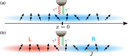
Figure 1: An infinite free-fermion chain with localized gain and loss processes acting at the center of the chain. Here $\gamma^{\pm}$ are the dissipation rates and $J=1$ the hopping. In (a) the chain is initially prepared in a homogeneous state $|\Psi\rangle$. Here we consider the case with $|\Psi\rangle$ being the fully occupied state $|F\rangle$, a Fermi sea with generic filling $k_{F}$ and the fermionic Néel state. In (b) the initial state is obtained by joining two semi-infinite homogeneous chains $L$ and $R$, prepared in two different states.

In this paper, we consider the infinite free-fermion chain defined by the tight-binding Hamiltonian

$$H=\sum_{x=-\infty}^{\infty}(c_{x}^{\dagger}c_{x+1}+c^{\dagger}_{x+1}c_{x})\,,$$ (1)

where $c_{x}^{\dagger},c_{x}$ are creation and annihilation operators at the different sites $x$ of the chain. They obey canonical anticommutation relations. The Hamiltonian in Eq. (1) becomes diagonal after taking a Fourier transform with respect to $x$. One can indeed define the fermionic operators $b_{k}$ as

$$b_{k}:=\sum_{x=-\infty}^{\infty}e^{-ikx}c_{x},\quad c_{x}=\int_{-\pi}^{\pi}\frac{dk}{2\pi}e^{ikx}b_{k}\,,$$ (2)

and in terms of these operators, Eq. (1) is equivalent to

$$H=\int_{-\pi}^{\pi}\frac{dk}{2\pi}\varepsilon_{k}b^{\dagger}_{k}b_{k}\,,\quad\varepsilon_{k}:=2\cos(k)\,.$$ (3)

The Hamiltonian $H$ conserves the particle number. At a fixed density $n_{f}=k_{F}/\pi$, the ground state can be obtained from the Fermi vacuum $\ket{0}$, by occupying the quasi-momenta $b_{k}$ with single-particle energies in $k\in[-k_{F},k_{F}]$, where $k_{F}$ is the Fermi momentum. For $n_{f}=1$ ($k_{F}=\pi$) one has the fully-filled state $|F\rangle$, which is a product state. For $0<k_{F}<\pi$ the ground state of (1) is instead critical, i.e., with power-law decaying correlation functions. For later convenience, we define here the group velocity $v_{k}$ of the fermions as

$$v_{k}:=\frac{d\varepsilon_{k}}{dk}=-2\sin(k)\,.$$ (4)

In addition to the Hamiltonian contribution, we consider a dynamics which is also affected by localized gain/loss processes at the center of the chain [see Fig. 1]. To account for these dissipative contributions, we exploit the formalism of quantum master equations Breuer and Petruccione (2002). The time-evolution of the system state $\rho_{t}$ is implemented by a Lindblad generator, through the following equation

$$\frac{d\rho_{t}}{dt}=-i[H,\rho_{t}]+\sum_{i=+,-}\left(L^{i}\rho_{t}L^{i\,\dagger}-\frac{1}{2}\{L^{i\,\dagger}L^{i},\rho_{t}\}\right)\,.$$ (5)

Here, the so-called jump operators $L^{i}$ are given by $L^{+}=\sqrt{\gamma^{+}}c^{\dagger}_{0}$ and $L^{-}=\sqrt{\gamma^{-}}c_{0}$ (see Fig. 1 for a pictorial definition), and account for gain and loss, with rates $\gamma^{+}$ and $\gamma^{-}$, respectively.

The relevant information about the system is contained in the fermionic two-point correlation functions

$$G_{x,y}(t):=\mathrm{Tr}(c^{\dagger}_{x}c_{y}\rho(t))\,.$$ (6)

The dissipative dynamics of this covariance matrix is obtained as

$$G(t)=e^{t\Lambda}G(0)e^{t\Lambda^{\dagger}}+\int_{0}^{t}dze^{(t-z)\Lambda}\Gamma^{+}e^{(t-z)\Lambda^{\dagger}},$$ (7)

with $G(0)$ being the matrix containing the initial correlations. The matrix $\Lambda$ is defined as

$$\Lambda=ih-\frac{1}{2}(\Gamma^{+}+\Gamma^{-}),$$ (8)

where $h=\delta_{|x-y|,1}$ implements the Hamiltonian contribution while $\Gamma^{\pm}=\gamma^{\pm}\delta_{x,0}$ account for the localized dissipative effects. The correlation functions $G_{x,y}$ in (7) satisfy the linear system of equations (we drop the explicit time dependence when this does not generate confusion)

$$\frac{dG_{x,y}}{dt}=i(G_{x+1,y}+G_{x-1,y}-G_{x,y+1}-G_{x,y-1})\\ -\frac{\gamma^{+}+\gamma^{-}}{2}(\delta_{x,0}G_{x,y}+\delta_{y,0}G_{x,y})+\gamma^{+}\delta_{x,0}\delta_{y,0}.$$ (9)

We mainly consider the loss process, setting $\gamma^{+}=0$ in (9) and (7). This is not a severe limitation since the knowledge of $G_{x,y}$ for $\gamma^{+}=0$ is sufficient to reconstruct $G_{x,y}$ also in cases of a nonzero $\gamma^{+}$ (see Appendix A). We also notice that equations of the type of (9) can be efficiently numerically solved by standard iterative methods, such as the Runge-Kutta method Press et al. (2007). This is especially useful to treat the case of non-quadratic Liouvillians, for instance, in the presence of dephasing or incoherent hopping Alba and Carollo (2021). In our case this is not necessary because the solution of (9) is given by (7). Indeed, Eq. (7) can be evaluated numerically after noticing that the matrix $\Lambda$ is $L\times L$, and it can be diagonalized with a computational cost ${\mathcal{O}}(L^{3})$. This allows to efficiently evaluate the integral in (7).

In the following sections we discuss the effect of gain/loss dissipation in several theoretically and experimentally relevant situations. We consider both equilibrium as well as out-of-equilibrium systems, i.e. after a quantum quench Polkovnikov et al. (2011); Eisert et al. (2015); Gogolin and Eisert (2016); D’Alessio et al. (2016); Calabrese et al. (2016). At equilibrium we are interested in understanding how the local dissipation affects the critical correlations of a homogeneous Fermi sea with arbitrary filling $0<k_{F}<\pi$. We also review the effect of losses in the non-critical state $|F\rangle$, which was discussed in Ref. Krapivsky et al., 2019. Furthermore, we consider the case in which the initial state is a product state that is however not an eigenstate of the Hamiltonian (1). In the absence of dissipation this is one of the paradigm of quantum quenches. The generic out-of-equilibrium dynamics ensuing from an initial product state is in fact highly nontrivial, as for instance reflected by the ballistic growth of bipartite entanglement. Interestingly, for integrable systems, this growth is due to the propagation of pairs of entangled quasiparticles Calabrese and Cardy (2005); Fagotti and Calabrese (2008); Alba and Calabrese (2017, 2018). Our setting thus allows us to investigate the interplay between localized dissipation and quench dynamics. For concreteness, we focus on the situation in which the initial state is the fermionic Néel state $|N\rangle:=\prod_{x\,\mathrm{even}}c^{\dagger}_{x}|0\rangle$, in which only every other site is occupied.

Finally, we consider quenches from inhomogeneous initial states obtained by joining two homogeneous Fermi seas with different Fermi levels $k_{F}^{l}$ and $k_{F}^{r}$ [see Fig. 1(b)]. The choice $k_{F}^{l}=\pi/2$ and $k_{F}^{r}=0$ corresponds to the so-called geometric quench Mossel et al. (2010), whereas $k_{F}^{l}=\pi$ and $k_{F}^{r}=0$ to the domain-wall quench Antal et al. (1999); Gobert et al. (2005); Antal et al. (2008); Allegra et al. (2016); Gamayun et al. (2020). The case with $k_{F}^{l}\neq k_{F}^{r}$ is particularly interesting since, in the absence of dissipation and at long times, a non-equilibrium steady state (NESS) emerges around the interface between the two parts of the chain. Such a NESS exhibits the critical correlations of a boosted Fermi sea Sabetta and Misguich (2013); Viti et al. (2016). Interestingly, the space-time profile of physical observables and of the von Neumann entropy in these setups admit an elegant field theory description in terms a Conformal Field Theory in a curved space Allegra et al. (2016); Dubail et al. (2017a); Brun and Dubail (2017); Dubail et al. (2017b); Brun and Dubail (2018); Ruggiero et al. (2019); Bastianello et al. (2020); Collura et al. (2020). For generic integrable systems without dissipation, similar inhomogeneous protocols can be studied by using the recently-developed Generalized Hydrodynamics Bertini et al. (2016); Castro-Alvaredo et al. (2016) (GHD).

III HOMOGENEOUS out-of-equilibrium states

In this section we discuss the effect of losses on homogeneous out-of-equilibrium states. To introduce the notation, we start by reviewing the quench from the fully-filled state Krapivsky et al. (2019) in section III.1. Note that, in the absence of dissipation there is no dynamics since such state is an eigenstate of Eq. (1). We will obtain analogous results in the more general context of section IV. In order to study the interplay between unitary and dissipative dynamics, in section III.2 we consider the quench from the fermionic Néel state.

III.1 Fully-filled state

Let us consider the out-of-equilibrium dynamics starting from the fully-filled state $|F\rangle$ defined as

$$|F\rangle:=\prod_{x=-\infty}^{\infty}c_{x}^{\dagger}|0\rangle\,.$$ (10)

The above state is a product state, with diagonal correlator $G_{x,y}$, given by

$$G_{x,y}(0)=\delta_{x,y}\,.$$ (11)

To solve (9) with $\gamma^{+}=0$ we employ a product ansatz Krapivsky et al. (2019) for $G_{x,y}$. Specifically, we take $G_{x,y}$ of the form

$$G_{x,y}=\sum_{k=-\infty}^{\infty}S_{k,x}\bar{S}_{k,y}\,,$$ (12)

where the bar denotes complex conjugation. A similar product ansatz will be used in section IV. The factorization as in (12) arises naturally when treating transport problems in free-fermion models Viti et al. (2016). Eq. (12) is consistent with (9) provided that $S_{k,x}$ satisfies

$$\frac{dS_{k,x}}{dt}=i[S_{k,x+1}+S_{k,x-1}]-\frac{\gamma^{-}}{2}\delta_{x,0}S_{k,x}\,.$$ (13)

From Eq. (11) we obtain as initial condition for $S_{k,x}$

$$S_{k,x}(0)=\delta_{x,k}\,.$$ (14)

Eq. (13) is conveniently solved by a combination of Laplace transform with respect to time and Fourier transform with respect to the space coordinate $x$. Let us define the Laplace transform $\widehat{S}_{k,x}(s)$ as

$$\widehat{S}_{k,x}(s)=\int_{0}^{\infty}dte^{-st}S_{k,x}(t).$$ (15)

This allows us to rewrite (13) as

$$s\widehat{S}_{k,x}-S_{k,x}(0)=i[\widehat{S}_{k,x+1}+\widehat{S}_{k,x-1}]-\frac{\gamma^{-}}{2}\delta_{x,0}\widehat{S}_{k,x}.$$ (16)

We can now perform the Fourier transform with respect to $x$, by defining

$$\widehat{S}_{k,q}=\sum_{x=-\infty}^{\infty}\widehat{S}_{k,x}e^{-iqx},$$ (17)

with $q\in[-\pi,\pi]$ being the momentum. From now on, we will use $\widehat{S}_{k,q/p}$ to indicate the Laplace and Fourier transform of $S_{k,x}$; instead $\widehat{S}_{k,x/y}$ will stand for the Laplace transform of $S_{k,x/y}$ only. After substituting in (16) and using the initial condition (14), we obtain

$$s\widehat{S}_{k,q}-e^{-iqk}=i\widehat{S}_{k,q}(e^{iq}+e^{-iq})-\frac{\gamma^{-}}{2}\widehat{S}_{k,x=0}.$$ (18)

The solution of (18) is straightforward, yielding

$$\widehat{S}_{k,q}=\big{[}e^{-iqk}-\frac{\gamma^{-}}{2}\widehat{S}_{k,x=0}\big{]}\frac{1}{s-2i\cos(q)}.$$ (19)

We note that $\widehat{S}_{k,x=0}$ is conveniently written as

$$\widehat{S}_{k,x=0}=\frac{1}{2\pi}\int_{-\pi}^{\pi}dq\widehat{S}_{k,q}.$$ (20)

We can now take the inverse Fourier transform in (19), and using that

$$\frac{1}{2\pi}\int_{-\pi}^{\pi}dq\frac{e^{iqx}}{s-2i\cos(q)}=\frac{1}{\sqrt{s^{2}+4}}\Big{(}\frac{2i}{s+\sqrt{s^{2}+4}}\Big{)}^{|x|},$$ (21)

we obtain

$$\widehat{S}_{k,x}=\frac{1}{\sqrt{s^{2}+4}}\Big{(}\frac{2i}{s+\sqrt{s^{2}+4}}\Big{)}^{|k-x|}\\ -\frac{\gamma^{-}/2}{(\gamma^{-}/2+\sqrt{s^{2}+4})\sqrt{s^{2}+4}}\Big{(}\frac{2i}{s+\sqrt{s^{2}+4}}\Big{)}^{|k|+|x|}.$$ (22)

Note the absolute value $|x|$ in the second term in (22). The last step is to take the inverse Laplace transform of (22). This is straightforward for the first term in Eq. (22), which accounts for the unitary part of the evolution, and gives a term $J_{|x-y|}(2t)$, with $J_{x}(t)$ the Bessel function of the first type. The second term in Eq. (22) encodes the effects of the losses. One can write Krapivsky et al. (2019)

$$S_{k,x}(t)=i^{|x-k|}J_{|x-k|}(2t)-\frac{\gamma^{-}}{2}i^{|x|+|k|}K_{|x|+|k|}(t).$$ (23)

Here $K_{|x|+|k|}$ is the inverse Laplace transform of the second term in Eq. (22). To determine $K_{|k|+|x|}$ analytically, one can use the inverse Laplace transform

$$D_{|x|}:={\mathcal{L}}^{-1}\Big{(}\frac{1}{\frac{\gamma^{-}}{2}+\sqrt{s^{2}+4}}\Big{(}\frac{2i}{s+\sqrt{s^{2}+4}}\Big{)}^{|x|}\Big{)}=i^{|x|}J_{|x|}(2t)\\ -i^{|x|}\frac{\gamma^{-}}{2}\int_{0}^{t}dze^{-\gamma^{-}z/2}\Big{(}\frac{t-z}{t+z}\Big{)}^{|x|/2}J_{|x|}(2\sqrt{t^{2}-z^{2}}),$$ (24)

together with the fact that

$${\mathcal{L}}^{-1}\Big{(}\frac{1}{{\sqrt{s^{2}+4}}}\Big{)}=J_{0}(2t).$$ (25)

This allows us to obtain the inverse Laplace of the second term in (22) as the convolution

$${\mathcal{L}}^{-1}\Big{(}\frac{1}{(\frac{\gamma^{-}}{2}+\sqrt{s^{2}+4})\sqrt{s^{2}+4}}\Big{(}\frac{2i}{s+\sqrt{s^{2}+4}}\Big{)}^{|k|+|x|}\Big{)}=\\ \int_{0}^{t}d\tau J_{0}(2(t-\tau))D_{|x|+|k|}(\tau),$$ (26)

with $D_{|x|+|k|}$ defined in Eq. (24). We anticipate that we will also employ Eq. (24) in section IV.

Here we are interested in the space-time scaling limit $x,k,t\to\infty$, with their ratio fixed. We define the two scaling variables $u,\xi_{x}$ as

$$u:=\frac{k}{2t},\quad\xi_{x}:=\frac{x}{2t}.$$ (27)

Since the initial state is homogeneous and the dissipation acts at $x=0$ we expect local observables, such as the fermionic density, to be even functions of $x$. Thus, we can restrict ourselves to $\xi_{x}>0$. The asymptotic behaviour of $J_{|x-k|}$ and $K_{|x|+|k|}$ is derived analytically Krapivsky et al. (2019) and is given by

$$J_{|x-k|}(2t)\simeq\\ \frac{\cos\big{[}2t\sqrt{1-(u-\xi_{x})^{2}}-2t|u-\xi_{x}|\arccos|u-\xi_{x}|-\frac{\pi}{4}\big{]}}{\sqrt{\pi t}\,\left[1-(u-\xi_{x})^{2}\right]^{1/4}},$$ (28)

which holds for $-1\leq u-\xi_{x}\leq 1$. For $u,\xi_{x}$ outside of this interval the asymptotic behavior of $J_{|x-k|}$ is subleading in the scaling limit. Similarly, one can show that Krapivsky et al. (2019)

$$K_{|x|+|k|}(t)\simeq\\ \frac{\cos\big{[}2t\sqrt{1-(\xi_{x}+|u|)^{2}}-2t(\xi_{x}+|u|)\arccos(\xi_{x}+|u|)-\frac{\pi}{4}\big{]}}{\sqrt{\pi t}\,\left[\gamma^{-}/2+2(\xi_{x}+|u|)\right]\left[1-(\xi_{x}+|u|)^{2}\right]^{1/4}},$$ (29)

which holds in the interval $-1\leq|u|+\xi_{x}\leq 1$. As it will be clear in section IV, the scaling behavior of $G_{x,y}$ will be given by a simple formula, in the limit $x,y,t\to\infty$ with $x/t$, $y/t$ fixed and $|x-y|/t\to 0$. On the other hand, we should stress that by using (23) together with the asymptotic expansions (28) and (29) it is possible to obtain the behavior of $G_{x,y}$ for large $x,y,t$ with arbitrary fixed ratios $\xi_{x}=x/(2t),\xi_{y}=y/(2t)$. However, as it is clear from (28) and (29) the result contains detailed information about the quench parameters and dissipation.

Let us consider the dynamics of the density profile $n_{x,t}$. We have

$$n_{x,t}=\sum_{k=-\infty}^{\infty}|S_{k,x}|^{2}.$$ (30)

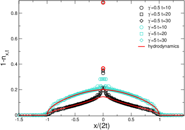
Figure 2: Density profile $n_{x,t}$ in a free fermion chain with localized losses. Here we plot $1-n_{x,t}$ versus $x/(2t)$, with $x$ the position with respect to the center of the chain and $t$ the time. The initial state of the chain is the fully occupied state $|F\rangle$. The symbols are exact numerical data for “strong” loss rate $\gamma^{-}=5$ and “weak” loss rate $\gamma^{-}=0.5$. Lines and the red circle at $x=0$ are the analytic results in the hydrodynamic limit.

The behavior of the density in the space-time scaling limit is obtained by using (28) and (29) in (30). Let us assume $\xi_{x}>0$. We obtain

$$n_{x,t}=1-\frac{\gamma^{-}}{\pi}\int_{\arcsin(x/(2t))}^{\pi/2}dq\frac{|v_{q}|}{(\frac{\gamma^{-}}{2}+|v_{q}|)^{2}}\,.$$ (31)

In deriving (31) we approximated the rapidly oscillating trigonometric functions in (28) and (29) with their time average. An important remark is that the derivation above is not valid near the origin at $x=0$, where the density profile exhibits a singularity. For $x=0$ from (22) we obtain

$$S_{k,0}(t)=i^{|k|}J_{|k|}(2t)\\ -i^{|k|}\frac{\gamma^{-}}{2}\int_{0}^{t}dze^{-\gamma^{-}z/2}\Big{(}\frac{t-z}{t+z}\Big{)}^{|k|/2}J_{|k|}(2\sqrt{t^{2}-z^{2}}).$$ (32)

In the scaling limit $k,t\to\infty$ with $u=k/(2t)$ fixed we have

$$\Big{(}\frac{t-z}{t+z}\Big{)}^{\frac{|k|}{2}}\simeq e^{-2|u|z}.$$ (33)

This implies

$$S_{k,0}(t)\simeq\frac{2i^{|k|}|u|}{\gamma^{-}/2+2|u|}J_{|k|}(2t).$$ (34)

By using the asymptotic expansion of the Bessel function (28) we obtain

$$n_{0,t}=\frac{1}{\pi}\int_{-\pi/2}^{\pi/2}dq\frac{|v_{q}|^{2}}{\big{(}\frac{\gamma^{-}}{2}+|v_{q}|\big{)}^{2}}.$$ (35)

We provide an alternative derivation of (31) and (35) in section IV. It is interesting to observe that from (31) in the limit of large loss rate $\gamma^{-}$ one obtains the Wigner semi-circle law as

$$n_{x,t}=1-\frac{1}{\gamma^{-}}\frac{8}{\pi}\sqrt{1-\frac{x^{2}}{4t^{2}}}.$$ (36)

The behavior in Eq. (36) appears also in the case of the out-of-equilibrium dynamics from the Néel state (see section III.2) and from inhomogeneous initial states (see section IV). Eq. (36) has a simple physical interpretation. Eq. (31) in the limit of large $\gamma$ can be rewritten as

$$n_{x,t}=1-\frac{1}{\gamma\pi}\int_{-\pi}^{\pi}dqv_{q}\Theta(v_{q}-x/t).$$ (37)

Now the integral in (37) describes the number of holes (equivalently, the absorbed fermions) that are emitted at the origin and at time $t$ arrive at position $x$. Importantly, since $dqv_{q}=d\epsilon$, this means that the hole is produced at a rate $\propto 1/\gamma$ with a uniform distribution in energy, i.e., at infinite temperature.

In the limit $\gamma^{-}\to\infty$ the density remains $n_{x,t}=1$. The total number of fermions absorbed at a generic time $t$ in the limit $\gamma^{-}\to\infty$ is given as

$$n_{a}:=\int_{-\infty}^{\infty}dx(1-n_{x,t})=\frac{8}{\gamma^{-}}t.$$ (38)

The number of fermions that are lost at the origin increases linearly with time. However, the rate goes to zero as $\gamma^{-}\to\infty$, which is consistent with the emergence of a Zeno effect. These results are checked in Fig. 2. The symbols are numerical data obtained by using (7) for $\gamma^{-}=0.5$ and $\gamma^{-}=5$. The different symbols correspond to different times. To highlight the scaling behavior we plot $1-n_{x,t}$ versus $x/(2t)$. All the data for different times collapse on the same curve. Note the singularity at $x=0$. Some corrections are visible only for very short times. The continuous lines are the analytical predictions (31) and (35), and are in perfect agreement with the numerical data.

III.2 Homogeneous Néel quench

Let us now discuss the effect of losses on an out-of-equilibrium state arising after the quantum quench from the fermionic Néel state. The Néel state $|N\rangle$ is defined as

$$|N\rangle:=\prod_{x\,\mathrm{even}}c_{x}^{\dagger}|0\rangle.$$ (39)

The initial correlation matrix reads as

$$G_{x,y}(0)=\delta_{x,y},\quad\mathrm{with}\,\,x\,\,\textrm{even}.$$ (40)

To proceed we impose that the solution of (9) is factorized as in Eq. (12). We obtain the same equation as in (13). The initial condition for $S_{k,x}$ is

$$S_{k,x}(0)=\delta_{x,k},\quad k\,\,\textrm{even}.$$ (41)

After performing a Laplace transform with respect to time we obtain (16). Now we can consider separately the cases of $k$ even and $k$ odd. Let us first start considering the case with $k$ odd. It is straightforward to check that (13) together with the initial condition (41) implies that $\widehat{S}_{k,n}=0$ for odd $k$. Thus we can restrict ourselves to even $k$. For $k$ even we have to distinguish the cases of even $x$ and odd $x$. We define $S^{e/o}_{k,x}$, where now $x=0,1,\dots,L/2$ labels the “unit cell” containing the sites $2x,2x+1$. These $S^{e/o}_{k,x}$ satisfy the set of equations

$$s\widehat{S}_{k,x}^{e}-\delta_{k,2x} =i[\widehat{S}_{k,x}^{o}+\widehat{S}_{k,x-1}^{o}]-\frac{\gamma^{-}}{2}\delta_{x,0}\widehat{S}^{e}_{k,x}$$ (42)

$$s\widehat{S}_{k,x}^{o} =i[\widehat{S}_{k,x}^{e}+\widehat{S}_{k,x+1}^{e}].$$ (43)

We define the Fourier transforms as

$$\widehat{S}_{k,q}^{e/o}=\sum_{x=-\infty}^{\infty}\widehat{S}^{e/o}_{k,x}e^{-iqx}.$$ (44)

Taking the Fourier transform in (42) and (43) we obtain

$$s\widehat{S}^{e}_{k,q}-e^{-iqk/2} =i\widehat{S}_{k,q}^{o}(1+e^{-iq})-\frac{\gamma^{-}}{2}\widehat{S}^{e}_{k,x=0}$$ (45)

$$s\widehat{S}^{e}_{k,q} =i\widehat{S}_{k,q}^{o}(1+e^{iq})$$ (46)

Similar manipulations as in section III.1 yield

$$\widehat{S}^{e}_{k,x}=\frac{1}{\sqrt{s^{2}+4}}\Big{(}\frac{2i}{s+\sqrt{s^{2}+4}}\Big{)}^{|k-2x|}\\ -\frac{\gamma^{-}}{2}\frac{1}{(\gamma^{-}/2+\sqrt{s^{2}+4})\sqrt{s^{2}+4}}\Big{(}\frac{2i}{s+\sqrt{s^{2}+4}}\Big{)}^{|k|+2|x|}\,,$$ (47)

and

$$\widehat{S}^{o}_{k,x}=i\int_{0}^{t}d\tau[\widehat{S}^{e}_{k,n}(\tau)+\widehat{S}^{e}_{k,x+1}(\tau)].$$ (48)

Eq. (47) is the same as for the quench from the ferromagnetic state (cf. (22)) discussed in section III.1, after redefining $x\to 2x$, i.e.,

$$S^{e}_{k,x}=S_{k,2x}^{|F\rangle},$$ (49)

with $S_{k,x}^{|F\rangle}$ given by (22). One can use (28) and (29) to obtain the correlators $G_{x,y}$ in the space-time scaling limit. We now discuss the dynamics of the density profile. We restrict ourselves to even sites $n^{e}_{n,t}$. This is because translation invariance is restored by the dynamics at long times and we expect the result for odd sites to be the same. We now have

$$n^{e}_{x,t}=\sum_{k=-\infty}^{\infty}|S^{e}_{2k,x}|^{2}.$$ (50)

One obtains

$$n^{e}_{x,t}=\frac{1}{2}-\frac{1}{2}\frac{\gamma^{-}}{\pi}\int_{\arcsin(x/(2t))}^{\pi/2}dq\frac{|v_{q}|}{\big{(}\frac{\gamma^{-}}{2}+|v_{q}|\big{)}^{2}}.$$ (51)

Note that this is the result obtained for the quench from the fully-filled state (see section III.1) divided by two. In addition, once again, the density profile is singular in $x=0$. The value of the density at $x=0$ is the half of that found in (35). In the absence of dissipation, i.e., for $\gamma^{-}=0$, the fermionic density is uniform and is given as $n_{x,t}=1/2$.

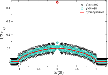
Figure 3: Density profile $n_{x,t}$ in a free fermion chain with local losses: Dynamics starting from the Néel state. We plot the shifted density $1/2-n_{x,t}$ versus $x/(2t)$. The symbols are exact numerical data for $\gamma^{-}=5$ and $t=98$ and $t=100$. Note the strong oscillations with time. Lines are the analytic results in the space-time scaling limit.

For strong dissipation, instead, one obtains

$$n^{e}_{x,t}=\frac{1}{2}-\frac{1}{\gamma^{-}}\frac{4}{\pi}\sqrt{1-\frac{x^{2}}{4t^{2}}},$$ (52)

which is reminiscent of the Wigner semicircle law in Eq. (36). It is useful to compare the results in (51) with numerical data. We present some benchmarks in Fig. 3. In the figure we show $1/2-n_{x,t}$ versus $x/(2t)$. The symbols are numerical results obtained by using (7). We only show data for $\gamma^{-}=5$. Strong oscillating corrections are present. They disappear in the long time limit $t\to\infty$. Similar corrections are also present in the unitary case, i.e., without dissipation. The continuous line is the analytic result in the space-time scaling limit. Despite the strong oscillations the agreement with the numerical data is satisfactory.

IV Quenches from inhomogeneous initial states

In this section we address the effect of losses in out-of-equilibrium dynamics starting from inhomogeneous initial states. We first discuss the so-called domain-wall quench in subsection IV.1. This can be straightforwardly treated by using the results of section III. We then discuss the generic situation in which the initial state is obtained by joining two Fermi seas with different fillings in subsection IV.2. We show that both the fermionic density and the correlation functions admit a simple hydrodynamic picture in the space-time scaling limit.

IV.1 Domain-wall quench

Let us consider the domain-wall initial state, in which the left part of the chain is fully filled, and the right one is empty. This situation has been intensely investigated in the past Antal et al. (1999); Bettelheim and Glazman (2012); Gobert et al. (2005); Allegra et al. (2016); Dubail et al. (2017a); Collura et al. (2018).

The full out-of-equilibrium dynamics ensuing from the domain-wall state is obtained by a slight modification of the method employed in section III. The same ansatz as in (12) holds true, with $S_{k,x}$ satisfying (13). The initial condition for $S_{k,x}$ is now

$$S_{k,x}(0)=\delta_{k,x}\Theta(-k),$$ (53)

where the Heaviside theta function $\Theta(-k)$ takes into account that at $t=0$ only the left part of the chain is fully occupied with fermions. In taking the Laplace and Fourier transforms of (12), we distinguish the case of $k\geq 0$ and $k<0$, obtaining

$$s\widehat{S}_{k,q}-e^{-iqk} =2i\widehat{S}_{q,k}\cos(q)-\frac{\gamma^{-}}{2}\widehat{S}_{k,x=0}\quad\textrm{for}\,k<0$$ (54)

$$s\widehat{S}_{k,q} =2i\widehat{S}_{q,k}\cos(q)-\frac{\gamma^{-}}{2}\widehat{S}_{k,x=0}\quad\textrm{for}\,k\geq 0.$$ (55)

The solution of the system above is straightforward and gives

$$\widehat{S}_{k,x}=\widehat{S}_{k,x}^{|F\rangle}\quad \textrm{for}\,k<0\,,$$ (56)

$$\widehat{S}_{k,x}=0\quad \textrm{for}\,k\geq 0,$$ (57)

where $\widehat{S}_{k,x}^{|F\rangle}$ (cf. (22)) is the same as for the quench from the fully-occupied state (see section III.1). Let us consider the density profile. For $x>0$ we obtain

$$n_{x,t}=\frac{1}{\pi}\int_{\arcsin(x/(2t))}^{\pi/2}dq\frac{|v_{q}|^{2}}{\big{(}\frac{\gamma^{-}}{2}+|v_{q}|\big{)}^{2}}.$$ (58)

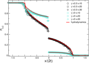
Figure 4: Density profile $n_{x,t}$ in a free fermion chain with localized losses: Dynamics starting from the domain-wall state. We plot $n_{x,t}$ versus $x/(2t)$. The symbols are exact numerical data. Lines are the analytic results in the space-time scaling limit.

For $x<0$ the density reads as

$$n_{x,t}=\frac{1}{\pi}\int^{\pi/2}_{\arcsin(x/(2t))}dq\\ +\frac{(\gamma^{-})^{2}}{4}\frac{1}{\pi}\int^{\pi/2}_{\arcsin(|x|/(2t))}dq\frac{1}{(\frac{\gamma^{-}}{2}+|v_{q}|)^{2}}.$$ (59)

Here $v_{q}$ is the fermion group velocity (4). Clearly, from (58) and (59) for $\gamma^{-}\to 0$ one recovers the expected result in the absence of dissipation. This corresponds to the first term in (59). Furthermore, in the limit of strong dissipation $\gamma^{-}\to\infty$, Eq. (58) is, again, reminiscent of the Wigner semicircle law. In particular, for $x>0$, from (59), one obtains that $n_{x,t}=16/(\gamma^{-}\pi)\sqrt{1-x^{2}/(4t^{2})}$.

In Fig. 4 we compare (58) and (59) with numerical results obtained from (7). We report data for strong dissipation $\gamma^{-}=5$ and weak one $\gamma^{-}=0.5$ and several times. The data show a perfect agreement when plotting $n_{x,t}$ versus $x/(2t)$. The scaling functions are consistent with the numerical results in the space-time scaling limit. Similarly to the quench from the Néel state we should stress that by using (28) and (29) it is possible to obtain the behavior of the generic fermionic correlator $G_{x,y}$ in the space-time scaling limit with arbitrary $\xi_{x}=x/(2t)$ and $\xi_{y}=y/(2t)$. Finally, we also stress that (59) can be rederived as a particular case of the double Fermi seas expansion that we will discuss in the next section.

IV.2 Inhomogeneous Fermi seas

In this section we discuss the situation in which two semi-infinite chains [see Fig 1(b)] are prepared in two Fermi seas at different fillings $k_{F}^{l}$ and $k_{F}^{r}$. The quench protocol is as follows. The two chains are prepared in the ground state of (1) with different fermionic densities, and with periodic boundary conditions. At $t=0$ the two chains are joined together. Note that due to the initial periodic boundary conditions on the two chains, this involves a “cut and glue” operation. The situation in which the two initial systems have open boundary conditions can be treated in a similar way, although we expect the out-of-equilibrium dynamics not to be dramatically affected by the choice of the boundary conditions. In the absence of dissipation, the out-of-equilibrium dynamics starting from two open chains that are joined together was obtained in Ref. Viti et al., 2016, in the space-time scaling limit. Note that by fixing $k_{F}^{l}=\pi$ and $k_{F}^{r}=0$, one obtains the domain-wall quench (see section IV.1). Instead, for $k_{F}^{r}=0$ and $k_{F}^{l}=\pi/2$ one has the so-called geometric quench Mossel et al. (2010), in which the ground state of a chain is let to expand in the vacuum.

It is straightforward to derive the initial correlation matrix as

$$G_{x,y}(0)=\frac{\sin(k_{F}^{r}(x-y))}{\pi(x-y)}\Theta(x)\Theta(y)\\ +\frac{\sin(k_{F}^{l}(x-y))}{\pi(x-y)}\Theta(-x)\Theta(-y),$$ (60)

where $\Theta(x)$ is the Heaviside theta function. Equation (60) is conveniently rewritten as

$$G_{x,y}(0)=\frac{1}{2\pi}\int_{-k_{F}^{l}}^{k_{F}^{l}}dke^{ik(x-y)}\Theta(-x)\Theta(-y)\\ +\frac{1}{2\pi}\int_{-k_{F}^{r}}^{k_{F}^{r}}dke^{ik(x-y)}\Theta(x)\Theta(y).$$ (61)

Crucially, Eq. (61) suggests that we can parametrize $G_{x,y}$ as

$$G_{x,y}=\frac{1}{2\pi}\int_{-k_{F}^{r}}^{k_{F}^{r}}dkS^{l}_{k,x}\bar{S}^{l}_{k,y}+\frac{1}{2\pi}\int_{-k_{F}^{l}}^{k_{F}^{l}}dkS^{r}_{k,x}\bar{S}^{r}_{k,y},$$ (62)

where $S_{k,x}^{l/r}$ have to be determined. Clearly, the ansatz (62) is similar to the one used in section (12). After substituting Eq. (62) in (9), we obtain that $S_{k,x}^{\scriptscriptstyle l/r}$ satisfy (13). The initial conditions are given as

$$S^{r/l}_{k,x}(0)=e^{ikx}\Theta(\pm x),$$ (63)

where the plus and minus signs are for $S^{r}_{k,x}$ and $S^{l}_{k,x}$, respectively. The Laplace and Fourier transforms of (62) read

$$\widehat{S}_{k,q}^{l/r}=\widehat{S}_{k,q}^{l/r,U}+\widehat{S}_{k,q}^{l/r,D},$$ (64)

where we separated the unitary part from the contribution of the dissipation, as stressed by the superscripts $U$ and $D$ in (64). Here we defined

$$\widehat{S}_{k,q}^{l,U} =\frac{1}{s-2i\cos(q)}\frac{1}{1-e^{i(q-k+i0)}}$$ (65)

$$\widehat{S}_{k,q}^{r,U} =-\frac{1}{s-2i\cos(q)}\frac{1}{1-e^{i(q-k-i0)}}$$ (66)

$$\widehat{S}_{k,q}^{l,D} =\int_{-\pi}^{\pi}\frac{dp}{2\pi}\frac{Z(p)}{1-e^{i(p-k+i0)}}$$ (67)

$$\widehat{S}_{k,q}^{r,D} =-\int_{-\pi}^{\pi}\frac{dp}{2\pi}\frac{Z(p)}{1-e^{i(p-k-i0)}}.$$ (68)

The function $Z(p)$ is defined as

$$Z(p)=-\frac{\frac{\gamma^{-}}{2}}{\frac{\gamma^{-}}{2}+\sqrt{s^{2}+4}}\frac{\sqrt{s^{2}+4}}{s-2i\cos(p)}\frac{1}{s-2i\cos(q)}.$$ (69)

The terms $\pm i0$ in the equations above are convergence factors, and their sign is chosen to impose the $\Theta(\pm x)$ in the initial conditions for $S_{k,x}^{l/r}$ (cf. (63)). From (62) it is clear that in order to determine $G_{x,y}$ one has to compute the integrals ${\mathcal{I}}^{l}$ and ${\mathcal{I}}^{r}$ defined as

$${\mathcal{I}}^{l}=\frac{1}{4\pi^{2}}\int_{-k^{l}_{F}}^{k^{l}_{F}}\frac{dk}{(1-e^{i(p-k+i0)})(1-e^{-i(q-k-i0)})}$$ (70)

$${\mathcal{I}}^{r}=\frac{1}{4\pi^{2}}\int_{-k^{r}_{F}}^{k^{r}_{F}}\frac{dk}{(1-e^{i(p-k-i0)})(1-e^{-i(q-k+i0)})}.$$ (71)

Similar integrals were discussed in Ref. Viti et al., 2016.

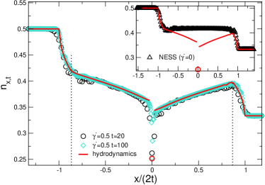
Figure 5: Density profile $n_{x,t}$ in a free fermion chain with localized losses with rate $\gamma^{-}$: Dynamics starting from the inhomogeneous state (see Fig. 1) obtained by joining two Fermi seas with $k_{F}^{l}=\pi/2$ and $k_{F}^{r}=\pi/3$. The symbols are exact numerical data for $\gamma^{-}=0.5$. Lines are the analytic results in the space-time scaling limit. Inset: The case without dissipation. Note the formation of the Non Equilibrium Steady State (NESS) at the interface between the two chains.

The integration over $k$ in Eqs. (70)-(71) can be performed easily in the complex plane. The derivation is as in Ref. Viti et al., 2016, and we do not report it here. We obtain

$$4\pi^{2}{\mathcal{I}}^{l/r}=\frac{i}{1-e^{i(p-q\pm i0)}}\Big{[}\ln\frac{e^{ik_{F}^{l}}-e^{iq}}{e^{-ik_{F}^{l}}-e^{iq}}\\ -\ln\frac{e^{ik_{F}^{l}}-e^{ip}}{e^{-ik_{F}^{l}}-e^{ip}}\mp 2\pi i\chi^{l/r}(p)\Big{]},$$ (72)

where the terms with $i0$ and $-i0$ in the exponential in (72) correspond to ${\mathcal{I}}^{l}$ and ${\mathcal{I}}^{r}$, respectively. Here the function $\chi^{l/r}(p)$ is one if $p$ is in the interval $[-k^{l/r}_{F},k^{l/r}_{F}]$, while it is zero otherwise.

The next step is to determine the large $x$ behavior of $S_{k,x}^{\scriptscriptstyle l/r,D}$. This requires to calculate the inverse Fourier transform of $Z(p)$ with respect to $q$ (cf. (69)) and its inverse Laplace transform with respect to $s$. More precisely, one has to determine the asymptotic behavior for large $x,t$ of

$$F_{x}^{D}:={\mathcal{L}}^{-1}\Big{(}\frac{1}{2\pi}\int_{-\pi}^{\pi}dqZ(p)e^{iqx}\Big{)}\,.$$ (73)

The derivation is reported it in Appendix B. Here we quote the final result, which reads

$$F_{x}^{D}(p)=\chi_{x}e^{2it\cos(p)+i|x||p|}r(p),$$ (74)

where $v_{p}$ is the fermions group velocity defined in (4). Here $\chi_{x}$ is defined as

$$\chi_{x}(p):=\Theta\Big{(}|v_{p}|-\frac{|x|}{t}\Big{)},$$ (75)

with $v_{p}$ the group velocity of the fermions (cf. (4)). In (74) we defined the reflection amplitude $r(p)$ as

$$r(p):=-\frac{\gamma^{-}}{2}\frac{1}{\frac{\gamma^{-}}{2}+|v_{p}|}.$$ (76)

Note that $r(p)$ appears in the scattering problem of a plane wave with a delta potential with imaginary strength Burke et al. (2020).

Finally, we discuss the behavior of $G_{x,y}$ in the space-time scaling limit for $t,x,y\to\infty$ with $x/(2t),y/(2t)$ fixed and $|x-y|/t\to 0$. Let us start by discussing the different contributions in Eqs. (65)-(66)-(67)-(68). We first consider the unitary contribution

$$\frac{1}{2\pi}\int_{-k_{F}^{l}}^{k_{F}^{l}}dkS_{k,x}^{l,U}\bar{S}_{k,y}^{l,U}=\\ \frac{1}{2\pi}\int_{-\pi}^{\pi}dpdqe^{2it\cos(p)-2it\cos{q}+ipx-iqy}\,{\mathcal{I}}^{l}(p,q).$$ (77)

The analysis is essentially the same as in Ref. Viti et al., 2016. Let us first consider the case with $x,y>0$. We employ the standard stationary phase approximation Wong (2001). In the large $t,x,y$ limit the stationary points in the double integral in (77) satisfy the equations

$$-2t\sin(p)+x=0$$ (78)

$$-2t\sin(q)+y=0$$ (79)

As it is clear from (78) and (79), in the space-time scaling, the integral (77) is dominated by the region with $p\to q$. Thus, we define $K:=(p+q)/2$ and $Q:=(p-q)$. In the limit $Q\to 0$ we have

$${\mathcal{I}}^{l/r}(p,q)=\mp\frac{1}{2\pi i}\frac{1}{Q\pm i0}\Theta(k_{F}^{l/r}-|K|),$$ (80)

where the term with $Q+i0$ refers to ${\mathcal{I}}^{l}$, and the one with $Q-i0$ to ${\mathcal{I}}^{r}$. By combining (80) with the well-known formula

$$\frac{1}{2\pi i}\int_{-\infty}^{\infty}dQ\frac{e^{iQx}}{Q\mp i0}=\pm\Theta(\pm x)$$ (81)

we obtain the relatively simple result

$$\frac{1}{2\pi}\int_{-k_{F}^{l}}^{k_{F}^{l}}dkS_{k,x}^{l,U}\bar{S}_{k,y}^{l,U}=\\ \int_{-k_{F}^{l}}^{k_{F}^{l}}\frac{dK}{2\pi}e^{iK(x-y)}\Theta\Big{(}2t\sin(K)-\frac{x+y}{2}\Big{)}\,.$$ (82)

This coincides with the result in Ref. Viti et al., 2016. The derivation of the remaining terms entering in the definition of $G_{x,y}$ (cf. (62) and (64)) is similar although more cumbersome due to the presence of the absolute values $|p|$ and $|q|$ in the integrands. We illustrate the main steps of the derivations in Appendix C. We obtain

$$G_{x,y}(t)=\int_{-k_{F}^{l}}^{k_{F}^{l}}\frac{dK}{2\pi}\Big{\{}e^{iK(x-y)}\Theta\Big{(}2t\sin(K)-\frac{x+y}{2}\Big{)}\\ +e^{iK(|x|-|y|)}\Theta(K)(\Theta(x)+\Theta(y))\chi_{x}\chi_{y}r\\ +\Theta(K)e^{iK(|x|-|y|)}\chi_{x}\chi_{y}r^{2}\Big{\}}+l\leftrightarrow r,$$ (83)

with $\chi_{x}$ as defined in (75). Note that $\chi_{x},\chi_{y}$ and $r$ are functions of $K$. Here the last term $l\leftrightarrow r$ is obtained by changing the integration boundaries as $k_{F}^{l}\to k_{F}^{r}$, and by replacing $K\to-K$ and $x,y\to-x,-y$ in the integrand in (83). Eq. (83) holds only in the space-time (hydrodynamic) limit $|x|,|y|,t\to\infty$ with fixed $x/(2t)\approx y/(2t)$. Note that, similar to the previous sections, the correlation matrix $G_{x,y}$ is singular at $x,y\to 0$. This happens because of fast oscillating terms in the limit $x\to\infty$ that cannot be neglected at $x\approx 0$. In the region $x/t,y/t\to 0$ one obtains

$$G_{x,y}=\int_{0}^{k_{F}^{l}}\frac{dK}{2\pi}(e^{iKx}+re^{iK|x|})(e^{-iKy}+re^{-iK|y|})\\ \int_{-k_{F}^{r}}^{0}\frac{dK}{2\pi}(e^{iKx}+re^{iK|x|})(e^{-iKy}+re^{-iK|y|}).$$ (84)

Before discussing the numerical checks of (83) it is useful to address its physical interpretation. To this purpose it is useful to focus on the dynamics of the fermionic density $G_{x,x}(t)$. Equation (83) is rewritten as

$$G_{x,x}=\int_{-\pi}^{\pi}\frac{dk}{2\pi}(n_{x,t}^{l}(k)+n_{x,t}^{r}(k)),$$ (85)

where $n^{(l/r)}_{x,t}(k)$ describe the evolution of the fermions with momentum $k$ originated in the initial left and right chains. As it is clear from (83), $n_{x,t}^{l}(k)$ is written as

$$n_{x,t}^{l}(k)=n_{0}^{l}(k)\Big{[}\Theta(-x)\Theta(k)(1+|r|^{2}\Theta(x+2t\sin(k)))\\ +\Theta(x)\Theta(k)\Theta(-x+2t\sin(k))|\tau|^{2}\\ +\Theta(-x)\Theta(-k)\Theta(-x+2t\sin(k))\Big{]}.$$ (86)

In (86) we defined the transmission amplitude $\tau(k)$ as

$$\tau(k):=\frac{v_{k}}{\frac{\gamma^{-}}{2}+|v_{k}|},$$ (87)

where $v_{k}$ is the fermion group velocity (cf. (4)). Note that $\tau^{2}+r^{2}\neq 1$, signaling that the evolution is not unitary. Note that $\tau(k)$ coincides with the transmission amplitude for the scattering with a delta potential with imaginary strength Burke et al. (2020). In (86), $n_{0}^{l}$ is the initial momentum distribution for the left chain $n_{0}^{l}=\Theta(k_{F}^{l}-|k|)$, and $r$ the reflection amplitude defined in (76). Now Eq. (86) has a simple physical interpretation. The first row in (86) describes the fermions moving towards the dissipative impurity and the scattered ones. The second row describes the fermions that are transmitted to the chain on the right at $x>0$. Finally, the last row accounts for the fermions that are in the left chain and are moving with negative velocity.

It is useful to check (83) and (84) against exact numerical data.

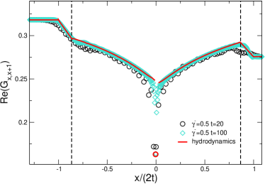
Figure 6: Depleted Non-Equilibrium Steady State (NESS). We show the dynamics of the off-diagonal correlator $\mathrm{Re}(G_{x,x+1})$ in the free fermion chain with localized losses. The data are exact numerical results for $\gamma^{-}=0.5$ for the infinite chain. We show results for the inhomogeneous initial state obtained by joining two Fermi seas with Fermi levels $k_{F}^{l}=\pi/2$ and $k_{F}^{r}=\pi/3$ (see Fig. 1 (b)). The curve is the result in the space-time scaling limit $t,x\to\infty$.

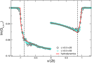
Figure 7: Depleted Non-Equilibrium Steady State (NESS). We show the dynamics of the fermion current $\mathrm{Im}(G_{x,x+1})$ in the free fermion chain with localized losses. The initial state and the dissipation are the same as in Fig. 6. The curve is the result in the space-time scaling limit $t,x\to\infty$.

This is discussed in Fig. 5. We plot the fermionic density $n_{x,t}$ versus the scaling variable $x/(2t)$. We consider the case with $k_{F}^{l}=\pi/2$ and $k_{F}^{r}=\pi/3$. Interestingly, in the absence of dissipation a Non-Equilibrium Steady State (NESS) emerges at the interface between the two chains with a flat density profile for $[-\sin(k_{F}^{r})\leq x/(2t)\leq\sin(k_{F}^{r})]$. The fermionic density in the flat region is the average density $(k_{F}^{l}+k_{F}^{r})/(2\pi)$. The case without dissipation is shown in the inset of Fig. 5. As it is clear from the main Figure, in the presence of losses the NESS is depleted. Also the density profile exhibits a clear asymmetry under $x\to-x$ with a discontinuity at $x=0$. Cusp-like features are present at $\pm k_{F}^{r}$. These are also present in the absence of dissipation Viti et al. (2016). Finally, we report in the Figure the analytic result in the space-time scaling limit (83). This is in perfect agreement with the numerical data. Note that the agreement is also good for $x=0$. The theoretical prediction for $x=0$ is given by (84) and it is reported as a circle in the Figure. Deviations are present near the singularities related to the Fermi momenta, similar to the non-dissipative case Viti et al. (2016), and are expected to vanish in the limit $x,t\to\infty$. Finally, we should mention that by imposing $k_{F}^{l}=k_{F}^{r}=k_{F}$ in (83) one obtains the space-time limit behavior of the correlator $G_{x,y}$ for the problem of a uniform Fermi sea with Fermi level $k_{F}$. This is explicitly discussed in Appendix D.

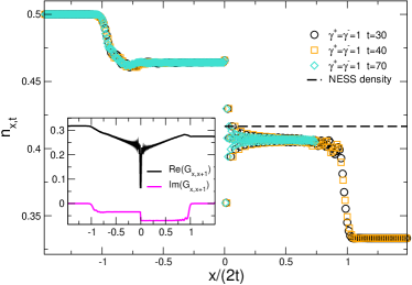
Figure 8: Broken NESS with balanced gain and losses. We show the fermionic density $n_{x,t}$ in the free fermion chain with gains and losses. The data are exact numerical results for $\gamma^{-}=\gamma^{+}=1$. The initial state is obtained by joining two Fermi seas with Fermi levels $k_{F}^{l}=\pi/2$ and $k_{F}^{r}=\pi/3$ (see Fig. 1 (b)). The dashed line is the NESS density $\pi(k_{F}^{l}+k_{F}^{r})/2$ in the absence of dissipation. In the inset we show the off-diagonal correlators $\mathrm{Re}(G_{x,x+1})$ and $\mathrm{Im}(G_{x,x+1})$.

In Fig. 6 and Fig. 7 we show the behavior of the off-diagonal correlation function $G_{x,x+1}$ in the space-time scaling limit. We present $\mathrm{Re}(G_{x,x+1})$ and $\mathrm{Im}(G_{x,x+1})$, which is the fermion current, separately. Similar to the density (see Fig. 5), the exact numerical data for $G_{x,x+1}$ obtained by numerically solving (9) collapse on the same curve when plotted as a function of $x/(2t)$, at least for large enough $x,t$. The scaling curve is perfectly described by the analytic result (83) and (84). Note that similar to Fig. 5 a singularity is present at $x=0$ in both Figures and the same cusp-like features at $x/(2t)=\sin(k_{F}^{r})$ can be observed. We observe that the current is zero for $|x|/(2t)\geq 1$, as expected since for $|x|/(2t)\geq 1$ the system is at equilibrium. Note also that $\mathrm{Im}(G_{x,x+1})<0$ for any $x$, and does not change its sign across the singularity. Finally, we should stress that on increasing $\gamma^{-}$ the transport between the two chains is suppressed, which is, again, a manifestation of the quantum Zeno effect. This is nicely encoded in the value assumed by the reflection and transmission coefficients; for $\gamma_{-}\to\infty$, we have $r(k)\to-1$ and $\tau(k)\to 0$.

To conclude we discuss an interesting effect that arises when one restores the gain dissipation. We consider the case of balanced gain/loss dissipation, i.e., with $\gamma^{+}=\gamma^{-}$. Our results are reported in Fig. 8. We focus on the density profile $n_{x,t}$ plotted versus $x/(2t)$. We fix $k_{F}^{l}=\pi/2$ and $k_{F}^{r}=\pi/3$ and $\gamma^{-}=\gamma^{+}=1$. Interestingly, as it is clear from Fig. 8 the density profile now exhibits a “broken” NESS structure. Specifically, two flat regions are visible for $-\sin(k^{r}_{F})\leq x\leq 0$ and $0<x\leq\sin(k^{r}_{F})$, with a step-like discontinuity at $x=0$. The dashed line in the figure shows the NESS density in the absence of dissipation. In the inset of Fig. 8 we report the behavior of the off-diagonal correlation $\mathrm{Re}(G_{x,x+1})$ and $\mathrm{Im}(G_{x,x+1})$, which show a nontrivial structure. We should mention that the behavior of the correlator in the presence of both gain and loss can be derived analytically by using the results in Appendix A, although we do not report its explicit expression.

V Conclusions

We have provided exact results on the out-of-equilibrium dynamics of free-fermion systems subject to localized gain/loss dissipation, playing the role of a dissipative defect. We considered different setups with both homogeneous and inhomogeneous initial states, and derived general results on the fermionic correlations $G_{x,y}(t)=\mathrm{Tr}(c^{\dagger}_{x}c_{y}\rho(t))$. Our findings hold in the space-time scaling limit (hydrodynamic limit) with $x,y,t\to\infty$, their ratios $\xi_{x}=x/(2t),\xi_{y}=y/(2t)$ being fixed. In this limit, we have shown that dissipation acts as an effective delta potential with momentum-dependent reflection and transmission amplitudes. For generic $\xi_{x},\xi_{y}$, the fermionic correlation functions depend on the details of the model. On the other hand, in the limit $\xi_{x}\approx\xi_{y}$, the dynamics of fermionic correlations is completely characterized by the initial fermionic occupations and the emergent reflection amplitude of the dissipative impurity.

Our results pave the way for several further studies. For instance, it would be interesting to extend them to more complicated free-fermion models, e.g., the transverse field Ising chain. Another interesting direction concerns the investigation of the effect of localized dissipation in free-bosonic systems Krapivsky et al. (2020). An intriguing question is how local dissipation affects the entanglement scaling at finite-temperature critical points. An ideal setup to explore this is provided by the so-called quantum spherical model, for which entanglement properties can be studied effectively Wald et al. (2020a, b); Alba (2021). Furthermore, it would be of interest to study how localized gain/loss dissipations may affect entanglement spreading, for instance, by studying the dynamics of the logarithmic negativity Vidal and Werner (2002); Plenio (2005); Calabrese et al. (2012); Shapourian and Ryu (2019) and comparing with the quasiparticle picture Alba and Calabrese (2019). In the absence of dissipation the entanglement dynamics has been investigated for both the geometric quench Alba and Heidrich-Meisner (2014); Vicari (2012); Nespolo and Vicari (2013) and the domain-wall quench Sabetta and Misguich (2013); Dubail et al. (2017a); Collura et al. (2020). Moreover, it is important to generalize our findings to the interacting case. Although this is a challenging task, the results in Ref. Bouchoule et al., 2020 provide first steps in this direction. It would be also interesting to understand whether it is possible to incorporate the effects of dissipation in the Conformal Field Theory framework put forward in Refs. Allegra et al., 2016; Dubail et al., 2017a or in the quantum GHD Ruggiero et al. (2020). Finally, it would be important to clarify the correlation structure of the broken NESS discussed in section IV.2, and to understand whether it can be observed experimentally.

VI Acknowledgements

We would like to thank Jérôme Dubail and Oleksandr Gamayun for useful discussions in related projects. V.A. acknowledges support from the European Research Council under ERC Advanced grant 743032 DYNAMINT. F.C. acknowledges support from the “Wissenschaftler-Rückkehrprogramm GSO/CZS” of the Carl-Zeiss-Stiftung and the German Scholars Organization e.V., as well as through the Deutsche Forschungsgemeinsschaft (DFG, German Research Foundation) under Project No. 435696605.

Appendix A Restoring fermion pumping

Here we discuss how to obtain the solution of the general equation (9) for $\gamma^{+}\neq 0$ and $\gamma^{-}\neq 0$ from the solution for the case with loss only, i.e., $\gamma^{+}=0$. The equation for $G_{x,y}$ to be solved is (9)

$$\frac{dG_{x,y}}{dt}=i(G_{x+1,y}+G_{x-1,y}-G_{x,y+1}-G_{x,y-1})\\ -\frac{\gamma^{+}+\gamma^{-}}{2}(\delta_{x,0}G_{x,y}+\delta_{y,0}G_{x,y})+\gamma^{+}\delta_{x,0}\delta_{y,0}.$$ (88)

Let us define as $\widetilde{G}_{x,y}$ the solution for the case with pure losses with effective loss rate $\gamma^{+}+\gamma^{-}$, i.e., the solution of (88) where we neglect the last term. We have

$$\frac{d\widetilde{G}_{x,y}}{dt}=i(\widetilde{G}_{x+1,y}+\widetilde{G}_{x-1,y}-\widetilde{G}_{x,y+1}-\widetilde{G}_{x,y-1})\\ -\frac{\gamma^{+}+\gamma^{-}}{2}(\delta_{x,0}\widetilde{G}_{x,y}+\delta_{y,0}\widetilde{G}_{x,y}).$$ (89)

Let us impose the initial condition as

$$\widetilde{G}_{x,y}(0)=G_{x,y}(0).$$ (90)

Now we define the correlator $G_{x,y}^{\prime}$ as the solution of the problem

$$\frac{dG^{\prime}_{x,y}}{dt}=i(G^{\prime}_{x+1,y}+G^{\prime}_{x-1,y}-G^{\prime}_{x,y+1}-G^{\prime}_{x,y-1})\\ -\frac{\gamma^{+}+\gamma^{-}}{2}(\delta_{x,0}G^{\prime}_{x,y}+\delta_{y,0}G^{\prime}_{x,y}),$$ (91)

with delta initial condition

$$G^{\prime}_{x,y}(0)=\delta_{x,0}\delta_{y,0}.$$ (92)

Clearly, $G_{x,y}^{\prime}$ is the solution of the problem with only losses with rate $\gamma^{+}+\gamma^{-}$ for the empty chain with one fermion at $x=0$. We can now write the solution $G_{x,y}$ of (88) as

$$G_{x,y}(t)=\gamma^{+}\int_{0}^{t}d\tau G^{\prime}_{x,y}(t-\tau)+\widetilde{G}_{x,y}(t).$$ (93)

By direct substitution, one can verify that Eq. (93) is the solution of (88) with initial condition (90).

Finally, by using the same strategy as in section III one obtains the correlator $G^{\prime}_{x,t}(t)$ as

$$G^{\prime}_{x,y}=S_{x}\bar{S}_{y},$$ (94)

where $S_{x}$ in the space-time scaling limit is given as Krapivsky et al. (2019)

$$S_{x}(t)\simeq\left\{\begin{array}[]{cc}\frac{2|\xi|}{\frac{\gamma^{+}+\gamma^{-}}{2}+2|\xi|}J_{|x|}(2t)&|x|>0\\ \\ -\frac{1}{(\gamma^{+}+\gamma^{-})^{2}t}J_{1}(2t)&x=0\end{array}\right.$$ (95)

where $\xi=x/(2t)$, and $J_{x}(t)$ are the Bessel functions of the first type.

Finally, we should remark that it is possible to extract from (93) the hydrodynamic behavior in the limit $x,y,t\to\infty$, similar to (84). Indeed, the term $\widetilde{G}_{x,y}$ in (93) is the same as in (84) except for a redefinition $\gamma^{-}\to\gamma^{+}+\gamma^{-}$. Let us now discuss the first term in (93). By using (95) in (93), one obtains

$$\gamma^{+}\int_{0}^{t}d\tau G^{\prime}_{x,y}(t-\tau)=\gamma^{+}t\int_{0}^{1}d\tau\frac{|x|/(\tau t)}{(\gamma^{+}+\gamma^{-})/2+|x|/(t\tau)}\\ \times\frac{|y|/(\tau t)}{(\gamma^{+}+\gamma^{-})/2+|y|/(t\tau)}J_{|x|}(2t\tau)J_{|y|}(2t\tau).$$ (96)

After using the integral representation for the Bessel function $J_{|x|}(2t)$ (see (104)) one obtains the three-dimensional integral

$$\gamma^{+}\int_{0}^{t}d\tau G^{\prime}_{x,y}(t-\tau)=\gamma^{+}t\int_{0}^{1}d\tau r^{\prime}_{x}(\tau)r^{\prime}_{y}(\tau)\\ \times\mathrm{Re}\int_{0}^{\pi}\frac{dz}{\pi}e^{iz|x|-2it\tau\sin(z)}\mathrm{Re}\int_{0}^{\pi}\frac{dk}{\pi}e^{ik|y|-2it\tau\sin(k)},$$ (97)

where we defined

$$r^{\prime}_{x}(\tau):=\frac{|x|/(\tau t)}{(\gamma^{+}+\gamma^{-})/2+|x/(\tau t)|}.$$ (98)

Now it is clear that in the limit $x,y,t\to\infty$ one can perform two of the integrals in (97) (for instance, the integral in $\tau$ and $p$) by using the stationary phase. A similar calculation is reported in Appendix B (see (105)). It is also useful to observe that in the limit $x,y,t\to\infty$ with $x/t,y/t$ fixed and $x/t\approx y/t$ one can replace $r^{\prime}_{x}\approx r^{\prime}_{y}$ in (97). By performing the integral, one should be able to obtain the hydrodynamic limit of (93) (similar to (84)).

Appendix B Effective delta potential of the dissipative impurity

In this section we derive the asymptotic behavior of $F_{x}^{D}$ (cf. (73)) in the limit $x\to\infty$. This will allow us to derive the reflection and transmission amplitudes of the effective delta potential associated with the dissipative impurity. First, the inverse Fourier transform of $Z(p)$ (cf. (69)) with respect to $q$ can be obtained analytically by using (21). Thus, to determine $F_{x}^{D}$ (cf. (73)) one has to calculate the inverse Laplace transform

$$F^{D}_{x}:={\mathcal{L}}^{-1}\Big{(}\frac{-\frac{\gamma^{-}}{2}}{\frac{\gamma^{-}}{2}+\sqrt{s^{2}+4}}\Big{(}\frac{2i}{s+\sqrt{s^{2}+4}}\Big{)}^{|x|}\frac{1}{s-2i\cos(p)}\Big{)}\,.$$ (99)

This can be obtained by using (24) and that

$${\mathcal{L}}^{-1}\Big{(}\frac{1}{s-2i\cos(p)}\Big{)}=e^{2it\cos(p)}.$$ (100)

Now we obtain

$$F_{x}^{D}=-\frac{i^{|x|}\gamma^{-}}{2}e^{2it\cos(p)}\Big{[}\int_{0}^{t}d\tau J_{|x|}(2\tau)e^{-2i\tau\cos(p)}-\frac{\gamma^{-}}{2}\int_{0}^{t}d\tau\\ \int_{0}^{\tau}dze^{-\gamma^{-}z/2}\Big{(}\frac{\tau-z}{\tau+z}\Big{)}^{\frac{|x|}{2}}J_{|x|}(2\sqrt{\tau^{2}-z^{2}})e^{-2i\tau\cos(p)}\Big{]}$$ (101)

We now consider the space-time scaling limit $x,t\to\infty$ with the ratio $\xi_{x}=x/(2t)$ fixed. In the scaling limit we have

$$\Big{(}\frac{\tau-z}{\tau+z}\Big{)}^{\frac{|x|}{2}}\simeq e^{-2|\xi_{x}|z}.$$ (102)

We can proceed as in section III.1 to obtain

$$F^{D}_{x}(p):=-\frac{\gamma^{-}}{2}I^{D}_{x}=\\ -\frac{\gamma^{-}}{2}i^{|x|}\int_{0}^{1}d\tau J_{|x|}(\tau t)e^{2it(1-\tau)\cos(p)}\frac{|x|}{\tau\frac{\gamma^{-}}{2}+\frac{|x|}{t}}.$$ (103)

Now we have to derive the large $x,t$ behavior of the integral $I_{x}^{D}$. To proceed, we employ the integral representation of the Bessel function $J_{n}(x)$ as

$$J_{x}(x\tau/\xi_{x})=\mathrm{Re}\int_{0}^{1}dze^{ix(\pi z-\tau/\xi_{x}\sin(\pi z))}.$$ (104)

One now has to determine the large $x$ behaviour of the double integral

$$I_{x}^{D}(p)=\frac{1}{2}i^{|x|}e^{2it\cos(p)}\int_{0}^{1}d\tau\int_{0}^{1}dz\\ [e^{i|x|(\pi z-\tau/|\xi_{x}|\sin(\pi z)-\tau/|\xi_{x}|\cos(p))}+z\to-z]\frac{|x|}{\tau\frac{\gamma^{-}}{2}+\frac{|x|}{t}},$$ (105)

which is obtained by using (104) in (103). The integral in (105) can be evaluated by using the two-dimensional stationary phase approximation Wong (2001). The stationary point for the first term in the square brackets is at

$$\tau^{*}=\frac{|\xi_{x}|}{|\sin(p)|},\quad z^{*}=\frac{|p|}{\pi}-\frac{1}{2}.$$ (106)

By imposing that the stationary point is in the integration domain, one obtains the condition

$$\frac{\pi}{2}\leq|p|\leq\pi-\arcsin(|\xi_{x}|).$$ (107)

The second term within the square brackets in (105) has a stationary point at

$$\tau^{*}=\frac{|\xi_{x}|}{|\sin(p)|},\quad z^{*}=\frac{1}{2}-\frac{|p|}{\pi}.$$ (108)

The condition that the stationary points is in the integration domain $[0,1]\times[0,1]$ gives the condition

$$\arcsin(|\xi_{x}|)\leq|p|\leq\frac{\pi}{2}.$$ (109)

The analysis above implies that $F_{n}^{D}(p)$ has a contribution $\propto 1/|x|$ for $\arcsin(|\xi_{x}|)\leq|p|\leq\pi-\arcsin(|\xi_{x}|)$. For values of $p$ outside of this interval the integral in (105) exhibits a faster decay with increasing $x$ and it does not contribute in the space-time scaling limit.

We now apply the stationary-phase approximation to (105). Given two generic functions $g(w)$ and $f(w)$ in two dimensions, the stationary phase method states that in the large $x$ limit one has Wong (2001)

$$\int_{\Omega}g(w)e^{ixf(w)}\\ \simeq g(w_{0})|\det H|^{-1/2}\exp\Big{(}ixf(w_{0})+i/4\pi\sigma\Big{)}\frac{2\pi}{x}.$$ (110)

Here $\Omega$ is the integration domain. In our case from (105) $\Omega$ is the square $\Omega=[0,1]\times[0,1]$. In (110) $H$ is the Hessian matrix, $\sigma$ denotes the signature of the eigenvalues of $H$, and $w_{0}$ is the stationary point, i.e., for which $\nabla_{w}f(w)=0$. One can show that in our case $\sigma=0$. Moreover, the two stationary points (106) and (108) give the same contribution. From (103) we obtain

$$|\det H|=\pi^{2}\frac{\sin^{2}(p)}{\xi_{x}^{2}}.$$ (111)

The phase factor in (110) reads

$$f(w_{0})=-\frac{\pi}{2}+|p|.$$ (112)

After using (112) (111) in (110) we obtain (74)

$$F_{x}^{D}(p)=-\frac{\gamma^{-}}{2}\frac{\chi_{x}}{\frac{\gamma^{-}}{2}+|v_{p}|}e^{2it\cos(p)+i|x||p|},$$ (113)

where we used that $v_{p}=-2\sin(p)$ (cf. (4)) and $\chi_{x}$ is defined in (75). The prefactor multiplying the exponential is the reflection amplitude $r(p)$ in (76). For $p$ such that $\chi_{x}=0$ the integral in (105) does not possess stationary points within the integration domain. Then, contributions originate from stationary points at the boundary of the domain and are subleading, i.e., they do not contribute in the space-time scaling limit. These contributions can be analyzed systematically within the stationary-phase approximation. Let us now briefly discuss their origin. We use the trivial identity Wong (2001)

$$\int_{\Omega}dwg(w)e^{ixf(w)}=-\frac{i}{x}\int_{\partial\Omega}ds(\vec{u}\cdot\hat{\nu})e^{ixf(w)}\\ +\frac{i}{x}\int_{\Omega}dw(\vec{\nabla}\cdot\vec{u})e^{ixf(w)},$$ (114)

where $\partial\Omega$ denotes the boundary of $\Omega$ and $\hat{\nu}$ is the unit vector pointing outward normal to $\partial\Omega$. In (114) $\vec{u}$ is defined as

$$\vec{u}=\frac{\vec{\nabla}f}{|\vec{\nabla}f|^{2}}g.$$ (115)

In the presence of a boundary stationary point, the first term in the right hand side in (114) gives a contribution $1/x^{3/2}$, whereas the last term is subleading.

Appendix C Double Fermi seas expansion: Some technical derivations

In this section we report the derivation of (83). Specifically, we first derive in detail the term

$$I_{x,y}:=\frac{1}{2\pi}\int_{-k_{F}^{l}}^{k_{F}^{l}}dkS_{k,x}^{l,U}\bar{S}_{k,y}^{l,D}=\\ \frac{1}{2\pi}\int_{-\pi}^{\pi}dpdqe^{2it\cos(p)-2it\cos(q)+ipx-i|q||y|}\\ \times{\mathcal{I}}^{l}(p,q)\chi_{y}(q)r(q).$$ (116)

This is obtained from (62) (65)(67) with (69)(70), and the asymptotic expansion (113). In (116), $r(q)$ is the reflection amplitude defined in (76), ${\mathcal{I}}^{l}$ is defined in (70), and $\chi_{y}(q)$ is given by (75).

Here we are interested in the space-time scaling limit $x,y,t\to\infty$ with $\xi_{x}=x/(2t)$ and $\xi_{y}=y/(2t)$ fixed and $|x-y|/t\to 0$. In this regime the integral in (116) is dominated by the region $q\approx p$. Thus, it is convenient to define $Q:=p-q$ and $K:=(p+q)/2$. By treating carefully the absolute value $|q|$ in (116), we can rewrite (116) as

$$I_{x,y}=\\ -\int_{-\pi/2}^{\pi/2}\frac{dK}{2\pi}\int_{-2\pi+2|K|}^{2K}dQe^{iK(x-|y|)+i((x+|y|)/2-2t\sin(K))Q}\\ \frac{1}{2\pi i(Q+i0)}\chi_{y}(K)r(K)\\ -\int_{\pi/2}^{\pi}\frac{dK}{2\pi}\int_{-2\pi+2K}^{2\pi-2K}dQe^{iK(x-|y|)+i((x+|y|)/2-2t\sin(K))Q}\\ \frac{1}{2\pi i(Q+i0)}\chi_{y}(K)r(K)\\ -\int_{-\pi/2}^{\pi/2}\frac{dK}{2\pi}\int_{2K}^{2\pi-2|K|}dQe^{iK(x+|y|)+i((x-|y|)/2-2t\sin(K))Q}\\ \frac{1}{2\pi i(Q+i0)}\chi_{y}(K)r(K)\\ -\int_{-\pi}^{-\pi/2}\frac{dK}{2\pi}\int_{2|K|-2\pi}^{2\pi-2|K|}dQe^{iK(x+|y|)+i((x-|y|)/2-2t\sin(K))Q}\\ \frac{1}{2\pi i(Q+i0)}\chi_{y}(K)r(K).$$ (117)

The first two rows correspond to $q>0$, the other two to $q<0$. In (117) we used that in the limit $q\approx p$ Eq. (80) holds. We now observe that in the first two integrals in (117) only the region with $K>0$ contribute, whereas the remaining two integrals get contributions from the region with $K<0$. The final result reads as

$$\frac{1}{2\pi}\int_{-k_{F}^{l}}^{k_{F}^{l}}dkS_{k,x}^{l,U}\bar{S}_{k,y}^{l,D}=\\ \int_{0}^{k_{F}^{l}}\frac{dK}{2\pi}e^{iK(x-|y|)}\Theta\Big{(}2t\sin(K)-\frac{x+|y|}{2}\Big{)}\chi_{y}r\\ +\int_{-k_{F}^{l}}^{0}\frac{dK}{2\pi}e^{iK(x+|y|)}\Theta\Big{(}2t\sin(K)-\frac{x-|y|)}{2}\Big{)}\chi_{y}r,$$ (118)

where we used (81). A similar calculation allows us to obtain

$$\frac{1}{2\pi}\int_{-k_{F}^{l}}^{k_{F}^{l}}dkS_{k,x}^{l,D}\bar{S}_{k,y}^{l,U}=\\ \int_{0}^{k_{F}^{l}}\frac{dK}{2\pi}e^{iK(|x|-y)}\Theta\Big{(}-\frac{|x|+y}{2}+2t\sin(K)\Big{)}\chi_{x}r\\ +\int_{-k_{F}^{l}}^{0}\frac{dK}{2\pi}e^{iK(-|x|-y)}\Theta\Big{(}-\frac{-|x|+y}{2}+2t\sin(K)\Big{)}\chi_{x}r.$$ (119)

We also have

$$\frac{1}{2\pi}\int_{-k_{F}^{l}}^{k_{F}^{l}}dkS_{k,x}^{l,D}\bar{S}_{k,y}^{l,D}=\\ \int_{0}^{k_{F}^{l}}\frac{dK}{2\pi}e^{iK(|x|-|y|)}\Theta\Big{(}2t\sin(K)-\frac{|x|+|y|}{2}\Big{)}\chi_{x}\chi_{y|}r^{2}\\ +\int_{-k_{F}^{l}}^{0}\frac{dK}{2\pi}e^{iK(-|x|+|y|)}\Theta\Big{(}2t\sin(K)-\frac{-|x|-|y|}{2}\Big{)}\chi_{x}\chi_{y}r^{2}$$ (120)

The expressions above can be simplified as follows. Let us consider the case with $x,y\neq 0$. We observe that in Eq. (118) we can neglect oscillating contributions in the limit $x,y\to\infty$. Eq. (118) becomes

$$\frac{1}{2\pi}\int_{-k_{F}^{l}}^{k_{F}^{l}}dkS_{k,x}^{l,U}\bar{S}_{k,y}^{l,D}=\int_{0}^{k_{F}^{l}}\frac{dK}{2\pi}e^{iK(|x|-|y|)}\\ \times\Theta\big{[}\mathrm{sign}(x)(v_{K}-|\xi_{x}|-|\xi_{y}|)\big{]}\chi_{y}r.$$ (121)

In a similar way we obtain that

$$\frac{1}{2\pi}\int_{-k_{F}^{l}}^{k_{F}^{l}}dkS_{k,x}^{l,D}\bar{S}_{k,y}^{l,U}=\int_{0}^{k_{F}^{l}}\frac{dK}{2\pi}e^{iK(|x|-|y|)}\\ \times\Theta\big{[}\mathrm{sign}(y)(v_{K}-|\xi_{x}|-|\xi_{y}|)\big{]}\chi_{x}r.$$ (122)

One should observe that (121) and (122) are nonzero only for $x>0$ and $y>0$, respectively. Finally, we observe that in (120) only the first term contributes. We obtain

$$\frac{1}{2\pi}\int_{-k_{F}^{l}}^{k_{F}^{l}}dkS_{k,x}^{l,D}\bar{S}_{k,y}^{l,D}=\int_{0}^{k_{F}^{l}}\frac{dK}{2\pi}e^{iK(|x|-|y|)}\\ \times\Theta\big{[}v_{K}-|\xi_{x}|-|\xi_{y}|\big{]}\chi_{x}\chi_{y}r^{2}.$$ (123)

By using that in the space-time scaling limit $|x-y|/t\to 0$, we can rewrite (121) as

$$\frac{1}{2\pi}\int_{-k_{F}^{l}}^{k_{F}^{l}}dkS_{k,x}^{l,U}\bar{S}_{k,y}^{l,D}=\\ \int_{0}^{k_{F}^{l}}\frac{dK}{2\pi}e^{iK(x-|y|)}\Theta(x)\chi_{x}\chi_{y}r.$$ (124)

Eq. (122) becomes

$$\frac{1}{2\pi}\int_{-k_{F}^{l}}^{k_{F}^{l}}dkS_{k,x}^{l,D}\bar{S}_{k,y}^{l,U}=\\ \int_{0}^{k_{F}^{l}}\frac{dK}{2\pi}e^{iK(|x|-y)}\Theta(y)\chi_{y}\chi_{x}r.$$ (125)

Finally, we have that (123) is rewritten as

$$\frac{1}{2\pi}\int_{-k_{F}^{l}}^{k_{F}^{l}}dkS_{k,x}^{l,D}\bar{S}_{k,y}^{l,D}=\\ \int_{0}^{k_{F}^{l}}\frac{dK}{2\pi}e^{iK(|x|-|y|)}\chi_{x}\chi_{y}r^{2}.$$ (126)

Let us comment on the terms with $S_{k,x}^{r}$ (see (62)). It is clear from the symmetry of the problem (see Fig. 1) that these coincide with (82) (124)(125) and (126) after replacing $k_{F}^{l}\to k_{F}^{r}$ and after changing $K\to-K$ and $x,y\to-x,-y$ in the integrands.

Appendix D Two equal Fermi seas: Direct derivation

In this section we present the direct derivation of the fermionic correlator $G_{x,y}$ for the free-fermion chain with only losses and $k_{F}^{l}=k_{F}^{r}=k_{F}$. This corresponds to the uniform Fermi sea as initial state. For a uniform state the calculations are somewhat easier than in section IV.2 because only the asymptotic behavior of $F_{x}^{D}(p)$ (cf. (73)) in the limit $x,t\to\infty$ is required, whereas the stationary phase approximation discussed in section IV.2 is not necessary. The result coincides with Eq. (83) after fixing $k_{F}^{l}=k_{F}^{r}=k_{F}$, confirming the correctness of the derivation in section IV.2.

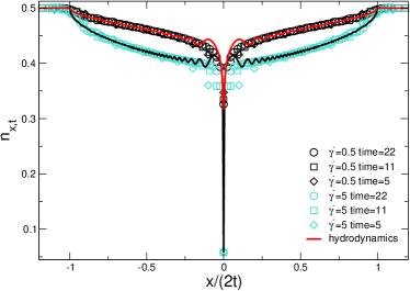
Figure 9: Density profile $n_{x,t}$ in a free fermion chain with local losses. The chain is prepared in a uniform Fermi sea at half filling, i.e., with $k_{F}=\pi/2$. The symbols are exact numerical data for $\gamma^{-}=0.5$ and $\gamma^{-}=5$. Lines are exact results in the space-time scaling limit. The oscillating correction are an artifact of the approximations and vanish in the space-time scaling limit.

For a Fermi sea with Fermi level $k_{F}$ the initial correlation matrix reads

$$G_{x,y}=\frac{\sin(k_{F}(x-y))}{\pi(x-y)}.$$ (127)

We now use the parametrization

$$G_{x,y}=\frac{1}{2\pi}\int_{-k_{F}}^{k_{F}}dkS_{k,x}\bar{S}_{k,y}$$ (128)

As in section IV.2, the equation for $S_{k,x}$ is

$$\frac{S_{k,x}}{dt}=i[S_{k,x+1}+S_{k,x-1}]-\frac{\gamma^{-}}{2}\delta_{x,0}S_{k,x}.$$ (129)

The initial condition reads as

$$S_{k,x}(0)=e^{ikx}.$$ (130)

We now use that

$$\sum_{x=-\infty}^{\infty}e^{ixz}=W(z):=2\pi\sum_{p=-\infty}^{\infty}\delta(z-2\pi p).$$ (131)

The Laplace/Fourier transforms of (129) read as

$$\widehat{S}_{k,q}=\widehat{S}^{U}_{k,q}+\widehat{S}_{k,q}^{D}.$$ (132)

Here we defined

$$\widehat{S}_{k,q}^{U}=\frac{1}{s-2i\cos(q)}W(k-q)$$ (133)

and

$$\widehat{S}_{k,q}^{D}=-\frac{\gamma^{-}}{4\pi}\int_{-\pi}^{\pi}dp\frac{W(k-p)}{\gamma^{-}/2+\sqrt{s^{2}+4}}\\ \times\frac{\sqrt{s^{2}+4}}{s-2i\cos(p)}\frac{1}{s-2i\cos(q)}.$$ (134)

Following the same steps as in section IV.2, we can rewrite $S_{k,n}^{D}$ and $S^{U}_{k,n}$ as

$$S_{k,x}^{U} =\frac{1}{2\pi}\int_{-\pi}^{\pi}dqe^{2it\cos(q)+iqx}W(k-q)$$ (135)

$$S_{k,y}^{D} =\frac{1}{2\pi}\int_{-\pi}^{\pi}dpW(k-p)e^{2it\cos(p)+i|x||p|}\chi_{x}r.$$ (136)

The integrations over $p$ and $q$ in (135) and (136) are straightforward, in contrast with section IV.2, because of the simple structure of $W(z)$ (cf. (131)). The net effect of the integration is to fix $q=k$ and $p=k$. The final result is given as

$$G_{x,y}(t)=\frac{1}{2\pi}\int_{-k_{F}}^{k_{F}}dk\Big{[}e^{ikx}+\chi_{x}re^{i|k||x|}\Big{]}\\ \times\Big{[}e^{-iky}+\chi_{y}re^{-i|k||y|}\Big{]}$$ (137)

It is interesting to observe that in (137) the time-dependent terms $e^{2it\cos(k)}$ drop out. The only time dependence is in the term $\chi_{|\xi_{x}|}$ and $\chi_{|\xi_{y}|}$. Finally, it is straightforward to check that in the space-time scaling limit $x,y,t\to\infty$ after neglecting oscillating terms Eq. (137) coincides with (83) with $k_{F}^{l}=k_{F}^{r}=k_{F}$.

In Fig. 9 we discuss exact numerical data for the fermionic density $n_{x,t}=G_{xx}$ obtained by solving numerically Eq. (9) with $\gamma^{+}=0$. We fix $k_{F}=\pi/2$. In the Figure we show results for both “strong” dissipation ($\gamma^{-}=5$) and “weak” dissipation ($\gamma^{-}=0.5$). Note that a singularity is present at $x=0$, as expected. Also, for $|x|/(2t)>1$ one has $n_{x,t}=1/2$. The continuous lines in Fig. 9 are (137). Note that oscillating corrections are present. These are an artifact of the derivation of (137). The corrections vanish in the limit $x,t\to\infty$ and Eq. (137) fully describes the numerical data.

References

- Degasperis et al. (1974) A. Degasperis, L. Fonda, and G. C. Ghirardi, Il Nuovo Cimento A (1965-1970) 21, 471 (1974).
- Misra and Sudarshan (1977) B. Misra and E. C. G. Sudarshan, Journal of Mathematical Physics 18, 756 (1977).
- Facchi and Pascazio (2002) P. Facchi and S. Pascazio, Phys. Rev. Lett. 89, 080401 (2002).
- Bernard et al. (2018) D. Bernard, T. Jin, and O. Shpielberg, EPL (Europhysics Letters) 121, 60006 (2018).
- Carollo et al. (2018) F. Carollo, J. P. Garrahan, and I. Lesanovsky, Phys. Rev. B 98, 094301 (2018).
- Popkov et al. (2018) V. Popkov, S. Essink, C. Presilla, and G. Schütz, Phys. Rev. A 98, 052110 (2018).
- Lin et al. (2013) Y. Lin, J. P. Gaebler, F. Reiter, T. R. Tan, R. Bowler, A. S. Sørensen, D. Leibfried, and D. J. Wineland, Nature 504, 415 (2013).
- Verstraete et al. (2009) F. Verstraete, M. M. Wolf, and J. Ignacio Cirac, Nature Physics 5, 633 (2009).
- Diehl et al. (2011) S. Diehl, E. Rico, M. A. Baranov, and P. Zoller, Nature Physics 7, 971 (2011).
- Vicari (2018) E. Vicari, Phys. Rev. A 98, 052127 (2018).
- Rossini and Vicari (2019a) D. Rossini and E. Vicari, Phys. Rev. A 99, 052113 (2019a).
- Nigro et al. (2019) D. Nigro, D. Rossini, and E. Vicari, Phys. Rev. A 100, 052108 (2019).
- Rossini and Vicari (2019b) D. Rossini and E. Vicari, Phys. Rev. B 100, 174303 (2019b).
- Di Meglio et al. (2020) G. Di Meglio, D. Rossini, and E. Vicari, Phys. Rev. B 102, 224302 (2020).
- Rossini and Vicari (2021) D. Rossini and E. Vicari, “Coherent and dissipative dynamics at quantum phase transitions,” (2021), arXiv:2103.02626 [cond-mat.stat-mech] .
- Breuer and Petruccione (2002) H. P. Breuer and F. Petruccione, The theory of open quantum systems (Oxford University Press, Great Clarendon Street, 2002).
- Prosen (2008) T. Prosen, New Journal of Physics 10, 43026 (2008).
- Prosen (2011) T. Prosen, Phys. Rev. Lett. 107, 137201 (2011).
- Prosen (2014) T. Prosen, Phys. Rev. Lett. 112, 030603 (2014).
- Prosen (2015) T. Prosen, Journal of Physics A: Mathematical and Theoretical 48, 373001 (2015).
- Žnidarič (2010) M. Žnidarič, Journal of Statistical Mechanics: Theory and Experiment 2010, L05002 (2010).
- Žnidarič (2011) M. Žnidarič, Phys. Rev. E 83, 011108 (2011).
- Medvedyeva et al. (2016) M. V. Medvedyeva, F. H. L. Essler, and T. Prosen, Phys. Rev. Lett. 117, 137202 (2016).
- Ilievski (2017) E. Ilievski, SciPost Phys. 3, 031 (2017).
- Buca et al. (2020) B. Buca, C. Booker, M. Medenjak, and D. Jaksch, “Dissipative bethe ansatz: Exact solutions of quantum many-body dynamics under loss,” (2020), arXiv:2004.05955 [cond-mat.stat-mech] .
- Bastianello et al. (2020) A. Bastianello, J. De Nardis, and A. De Luca, Phys. Rev. B 102, 161110 (2020).
- Essler and Piroli (2020) F. H. L. Essler and L. Piroli, Phys. Rev. E 102, 062210 (2020).
- Ziolkowska and Essler (2020) A. A. Ziolkowska and F. H. Essler, SciPost Phys. 8, 44 (2020).
- Sieberer et al. (2016) L. M. Sieberer, M. Buchhold, and S. Diehl, Reports on Progress in Physics 79, 96001 (2016).
- Bertini et al. (2016) B. Bertini, M. Collura, J. De Nardis, and M. Fagotti, Phys. Rev. Lett. 117, 207201 (2016).
- Castro-Alvaredo et al. (2016) O. A. Castro-Alvaredo, B. Doyon, and T. Yoshimura, Phys. Rev. X 6, 041065 (2016).
- Bouchoule et al. (2020) I. Bouchoule, B. Doyon, and J. Dubail, SciPost Phys. 9, 44 (2020).
- Friedman et al. (2020) A. J. Friedman, S. Gopalakrishnan, and R. Vasseur, Physical Review B 101 (2020).
- de Leeuw et al. (2021) M. de Leeuw, C. Paletta, and B. Pozsgay, “Constructing integrable lindblad superoperators,” (2021), arXiv:2101.08279 [cond-mat.stat-mech] .
- Nardis et al. (2021) J. D. Nardis, S. Gopalakrishnan, R. Vasseur, and B. Ware, “Stability of superdiffusion in nearly integrable spin chains,” (2021), arXiv:2102.02219 [cond-mat.stat-mech] .
- Calabrese and Cardy (2005) P. Calabrese and J. Cardy, Journal of Statistical Mechanics: Theory and Experiment 2005, P04010 (2005).
- Fagotti and Calabrese (2008) M. Fagotti and P. Calabrese, Phys. Rev. A 78, 010306 (2008).
- Alba and Calabrese (2017) V. Alba and P. Calabrese, Proceedings of the National Academy of Sciences of the United States of America 114 (2017), 10.1073/pnas.1703516114.
- Alba and Calabrese (2018) V. Alba and P. Calabrese, SciPost Phys. 4, 17 (2018).
- Alba and Carollo (2021) V. Alba and F. Carollo, Phys. Rev. B 103, L020302 (2021).
- Maity et al. (2020) S. Maity, S. Bandyopadhyay, S. Bhattacharjee, and A. Dutta, Phys. Rev. B 101, 180301 (2020).
- Dolgirev et al. (2020) P. E. Dolgirev, J. Marino, D. Sels, and E. Demler, Phys. Rev. B 102, 100301 (2020).
- Jin et al. (2020) T. Jin, M. Filippone, and T. Giamarchi, Phys. Rev. B 102, 205131 (2020).
- Maimbourg et al. (2020) T. Maimbourg, D. M. Basko, M. Holzmann, and A. Rosso, “Bath-induced zeno localization in driven many-body quantum systems,” (2020), arXiv:2009.11784 [cond-mat.stat-mech] .
- Fröml et al. (2019) H. Fröml, A. Chiocchetta, C. Kollath, and S. Diehl, Phys. Rev. Lett. 122, 040402 (2019).
- Tonielli et al. (2019) F. Tonielli, R. Fazio, S. Diehl, and J. Marino, Phys. Rev. Lett. 122, 040604 (2019).
- Fröml et al. (2020) H. Fröml, C. Muckel, C. Kollath, A. Chiocchetta, and S. Diehl, Phys. Rev. B 101, 144301 (2020).
- Krapivsky et al. (2019) P. L. Krapivsky, K. Mallick, and D. Sels, Journal of Statistical Mechanics: Theory and Experiment 2019, 113108 (2019).
- Krapivsky et al. (2020) P. L. Krapivsky, K. Mallick, and D. Sels, Journal of Statistical Mechanics: Theory and Experiment 2020, 63101 (2020).
- Rosso et al. (2020) L. Rosso, F. Iemini, M. Schirò, and L. Mazza, SciPost Phys. 9, 91 (2020).
- Vernier (2020) E. Vernier, SciPost Phys. 9, 49 (2020).
- Gericke et al. (2008) T. Gericke, P. Würtz, D. Reitz, T. Langen, and H. Ott, Nature Physics 4, 949 (2008).
- Brazhnyi et al. (2009) V. A. Brazhnyi, V. V. Konotop, V. M. Pérez-García, and H. Ott, Phys. Rev. Lett. 102, 144101 (2009).
- Zezyulin et al. (2012) D. A. Zezyulin, V. V. Konotop, G. Barontini, and H. Ott, Phys. Rev. Lett. 109, 020405 (2012).
- Barontini et al. (2013) G. Barontini, R. Labouvie, F. Stubenrauch, A. Vogler, V. Guarrera, and H. Ott, Phys. Rev. Lett. 110, 035302 (2013).
- Patil et al. (2015) Y. S. Patil, S. Chakram, and M. Vengalattore, Phys. Rev. Lett. 115, 140402 (2015).
- Labouvie et al. (2016) R. Labouvie, B. Santra, S. Heun, and H. Ott, Phys. Rev. Lett. 116, 235302 (2016).
- Lebrat et al. (2019) M. Lebrat, S. Häusler, P. Fabritius, D. Husmann, L. Corman, and T. Esslinger, Phys. Rev. Lett. 123, 193605 (2019).
- Corman et al. (2019) L. Corman, P. Fabritius, S. Häusler, J. Mohan, L. H. Dogra, D. Husmann, M. Lebrat, and T. Esslinger, Phys. Rev. A 100, 053605 (2019).
- Viti et al. (2016) J. Viti, J. M. Stéphan, J. Dubail, and M. Haque, Epl 115, 40011 (2016), arXiv:1507.08132 .
- Mossel et al. (2010) J. Mossel, G. Palacios, and J.-S. Caux, Journal of Statistical Mechanics: Theory and Experiment 2010, L09001 (2010).
- Antal et al. (1999) T. Antal, Z. Rácz, A. Rákos, and G. M. Schütz, Phys. Rev. E 59, 4912 (1999).
- Sabetta and Misguich (2013) T. Sabetta and G. Misguich, Phys. Rev. B 88, 245114 (2013).
- Press et al. (2007) W. Press, S. Teukolsky, W. Vetterling, and B. Flannery, Numerical Recipes: The Art of Scientific Computing, 3rd ed. (Cambridge University Press, 2007).
- Polkovnikov et al. (2011) A. Polkovnikov, K. Sengupta, A. Silva, and M. Vengalattore, Rev. Mod. Phys. 83, 863 (2011).
- Eisert et al. (2015) J. Eisert, M. Friesdorf, and C. Gogolin, Nature Phys. 11, 124 (2015).
- Gogolin and Eisert (2016) C. Gogolin and J. Eisert, Rep. Progr. Phys. 79, 056001 (2016).
- D’Alessio et al. (2016) L. D’Alessio, Y. Kafri, A. Polkovnikov, and M. Rigol, Adv. Phys. 65, 239 (2016).
- Calabrese et al. (2016) P. Calabrese, F. H. L. Essler, and G. Mussardo, J. Stat. Mech. 2016, 64001 (2016).
- Gobert et al. (2005) D. Gobert, C. Kollath, U. Schollwöck, and G. Schütz, Phys. Rev. E 71, 036102 (2005).
- Antal et al. (2008) T. Antal, P. L. Krapivsky, and A. Rákos, Phys. Rev. E 78, 061115 (2008).
- Allegra et al. (2016) N. Allegra, J. Dubail, J.-M. Stéphan, and J. Viti, Journal of Statistical Mechanics: Theory and Experiment 2016, 53108 (2016).
- Gamayun et al. (2020) O. Gamayun, O. Lychkovskiy, and J.-S. Caux, SciPost Phys. 8, 36 (2020).
- Dubail et al. (2017a) J. Dubail, J.-M. Stéphan, J. Viti, and P. Calabrese, SciPost Phys. 2, 002 (2017a).
- Brun and Dubail (2017) Y. Brun and J. Dubail, SciPost Phys. 2, 012 (2017).
- Dubail et al. (2017b) J. Dubail, J.-M. Stéphan, and P. Calabrese, SciPost Phys. 3, 019 (2017b).
- Brun and Dubail (2018) Y. Brun and J. Dubail, SciPost Phys. 4, 37 (2018).
- Ruggiero et al. (2019) P. Ruggiero, Y. Brun, and J. Dubail, SciPost Phys. 6, 51 (2019).
- Collura et al. (2020) M. Collura, A. De Luca, P. Calabrese, and J. Dubail, Phys. Rev. B 102, 180409 (2020).
- Bettelheim and Glazman (2012) E. Bettelheim and L. Glazman, Phys. Rev. Lett. 109, 260602 (2012).
- Collura et al. (2018) M. Collura, A. De Luca, and J. Viti, Phys. Rev. B 97, 081111 (2018).
- Burke et al. (2020) P. C. Burke, J. Wiersig, and M. Haque, Phys. Rev. A 102, 012212 (2020).
- Wong (2001) R. Wong, Asymptotic Approximations of Integrals (Society for Industrial and Applied Mathematics, 2001).
- Wald et al. (2020a) S. Wald, R. Arias, and V. Alba, Journal of Statistical Mechanics: Theory and Experiment 2020 (2020a), 10.1088/1742-5468/ab6b19.
- Wald et al. (2020b) S. Wald, R. Arias, and V. Alba, Physical Review Research 2, 043404 (2020b).
- Alba (2021) V. Alba, SciPost Phys. 10, 56 (2021).
- Vidal and Werner (2002) G. Vidal and R. F. Werner, Phys. Rev. A 65, 032314 (2002).
- Plenio (2005) M. B. Plenio, Phys. Rev. Lett. 95, 090503 (2005).
- Calabrese et al. (2012) P. Calabrese, J. Cardy, and E. Tonni, Phys. Rev. Lett. 109, 130502 (2012).
- Shapourian and Ryu (2019) H. Shapourian and S. Ryu, Phys. Rev. A 99, 022310 (2019).
- Alba and Calabrese (2019) V. Alba and P. Calabrese, EPL (Europhysics Letters) 126, 60001 (2019).
- Alba and Heidrich-Meisner (2014) V. Alba and F. Heidrich-Meisner, Phys. Rev. B 90, 075144 (2014).
- Vicari (2012) E. Vicari, Phys. Rev. A 85, 062324 (2012).
- Nespolo and Vicari (2013) J. Nespolo and E. Vicari, Phys. Rev. A 87, 032316 (2013).
- Ruggiero et al. (2020) P. Ruggiero, P. Calabrese, B. Doyon, and J. Dubail, Phys. Rev. Lett. 124, 140603 (2020).