Strong coupling effects in quantum thermal transport with the reaction coordinate method

Abstract

We present a semi-analytical approach for studying quantum thermal energy transport beyond the weak system-bath coupling regime. Our treatment, which results in a renormalized, effective Hamiltonian model is based on the reaction coordinate method. In our technique, applied to the nonequilibrium spin-boson model, a collective coordinate is extracted from each environment and added into the system to construct an enlarged system. After performing additional Hamiltonian’s truncation and transformation, we attain an effective two-level system with renormalized parameters, which is weakly coupled to its environments, thus can be simulated using a perturbative Markovian quantum master equation approach. We compare the heat current characteristics in our method to other techniques, and demonstrate that we properly capture strong system-bath signatures such as the turnover behavior of the heat current as a function of system-bath coupling strength. We further investigate the thermal diode effect and demonstrate that strong couplings moderately improve the rectification ratio relative to the weak coupling limit. The effective Hamiltonian method that we developed here offers fundamental insight into the strong coupling behavior, and is computationally economic. Applications of the method towards studying quantum thermal machines are anticipated.

I Introduction

Nonequilibrium dissipative quantum systems play a central role in quantum technologies. However, simulating the dynamics and transport properties of open quantum systems is challenging given the important role of the surrounding environment. Perturbative treatments in the language of Green’s functions diventra or quantum master equations (QMEs) Breuer ; Nitzan ; Strunz20 have proved fruitful, bringing much insights. QME methods are perturbative in the coupling energy of the system to its surroundings, further typically assuming a Markovian-memoryless system’s dynamics. Particularly for second-order QMEs, the rate constants responsible for transitions between quantum states are linear in the system-bath interaction energy (quantified e.g. by the reorganization energy). Nevertheless, many open-system processes fall outside the regime of validity of perturbation techniques, ranging from biological charge and exciton transport processes Thorwart ; Coker to quantum devices Nori .

In contrast to the linear-monotonous nature of the weak coupling regime, strong system-bath couplings can enact rich functional behavior relying on involved phenomena such as time nonlocal effects, cooperative interactions between thermal baths, and the buildup of correlations between a system and its surroundings. Significant efforts are currently directed to understand—and harness—the nontrivial outcome of strong system-bath couplings on the performance of quantum heat machines; a small sample of such studies include Strasberg_2016 ; Hava18 ; Newman ; Goold ; Misha ; Wiedmann2020 ; Motz2018 .

The nonequilibrium spin-boson (SB) model, with a two-level system (spin) coupled to two independent harmonic-oscillator (HO) baths was suggested for exploring the fundamentals of thermal energy transport in anharmonic nanojunctions PRL05 ; QME06 . Remarkably, the model was recently realized in superconducting quantum circuits demonstrating a thermal diode effect PekolaE . The heat current in the SB model displays a turnover behavior at strong coupling: While in the weak coupling limit the steady state heat current grows monotonically with the system-bath interaction energy, at strong coupling the current is suppressed ThossMCTDH ; NIBA11 ; Nazim14 ; NIBA14 ; ARPC ; Aurell2020 .

Numerous techniques were developed to investigate the thermal transport characteristics of the nonequilibrium SB model, specifically the turnover behavior mentioned above, by going beyond the weak-coupling Born-Markov Redfield (BMR) equation. For example, the non-interacting blip approximation (NIBA), which is perturbative in the tunneling splitting (nonadiabatic parameter) can properly describe strong system-bath coupling effects for Ohmic baths PRL05 ; QME06 ; NIBA11 ; NIBA14 ; Aurell2019 . To interpolate between the weak-coupling Born-Markov Redfield equation and the strong-coupling NIBA for general spectral functions, a nonequilibrium polaron-transformed Redfield equation has been developed in Refs. Cao1 ; Cao2 . Keldysh nonequilibrium Green’s function (NEGF) methods were furthermore developed for the SB model in Refs. ThossNEGF ; WuNEGF ; NJP17 ; PT-NEGF17 .

Beyond perturbative methods, numerically-exact techniques, originally developed to study the dissipative dynamics of the spin-boson model, were extended to investigate the behavior of the heat current in steady state. This includes simulations with the multi-layer multi-configuration Hartree approach ThossMCTDH ; MCTDHH , iterative influence functional path integral techniques Segal13 ; Nazim14 ; PI , quantum Monte Carlo Saito1 ; Saito2 and the hierarchical equation of motion HEOM1 ; HEOM2 ; HEOM3 ; HEOM4 . Other treatments involve semiclassical Kelly , mixed quantum-classical approximations mixed1 ; mixed2 ; mixed3 , and chain mapping approaches Plenio1 ; Plenio2 ; Plenio3 ; Poletti2020 .

The reaction coordinate (RC) method offers an alternative, balanced approach between low-order perturbation theory treatments and brute-force numerical methods. In this semi-analytic method, a collective coordinate of the bath, termed reaction coordinate, is identified and included into the quantum system. This step, or mapping, is exact. Since the RC incorporates system-bath interaction energies, the dynamics of the enlarged, “super-system” captures effects beyond weak coupling and beyond the Markovian approximation even when evolved approximately using a second-order Markovian QME PlenioProof ; Francesco20 . Obviously, the principle of the RC method can be generalized with several discrete modes extracted from the baths and included either as part of the system or as a primary non Markovian environment, further coupled to a secondary Markovian bath Gauger15 ; Eisfeld15 ; Nori19 ; PlenioProof ; Francesco20 ; Plenio1 ; Plenio2 ; Plenio3 ; Poletti2020 .

Apart from its computational simplicity, the reaction-coordinate quantum master equation (RC-QME) procedure can bring insights on the system’s dynamics and the evolution of system-environment correlations NazirPRA14 ; Nazir16 . The RC-QME method has been applied onto both bosonic and fermionic systems GernotF ; GernotF2 ; Nazir18 ; GalperinF . Furthermore, recent studies with this method examined the role of strong coupling effects in the performance of autonomous Strasberg_2016 and four-stroke Nazir18 thermal machines.

In this paper we develop, test, and benchmark a RC quantum master equation method for nonequilibrium quantum heat transport problems. Beyond numerical simulations, our objective is to gain insight on the role of strong system-bath couplings in the operation of thermal devices.

The turnover behavior of the heat current with system-bath coupling energy has been demonstrated with several methods, interpreted using a picture analogous to polaron transformation PRL05 ; QME06 ; NIBA11 ; NIBA14 ; Cao1 ; Cao2 . Here, we explain the turnover behavior of the heat current with an alternative picture: Employing the RC framework, we show that with a series of transformations and truncation we can convert the original-standard spin-boson model with strong system-bath couplings into an effective spin-boson model (EFF-SB). In the new model, the spin splitting is renormalized (suppressed) with coupling energy. Other parameters that are renormalized or transformed are the coupling parameters of the spin to the heat baths and the reservoirs’ spectral density functions. The new, effective SB model captures nontrivial-nonlinear effects—such as the suppression of the heat current at strong coupling—even at the level of a Markovian second-order QME. Overall, our approach handles the nontrivial strong coupling regime with minimal cost.

Our work addresses the following questions regarding heat transport in nanojunctions: (i) What is the origin of the heat current suppression at strong coupling? (ii) How does the current scale with different system’s parameters? (iii) What is the extent of the thermal rectification (diode) behavior? Does strong coupling assist the rectification effect?

The paper is organized as follows. In Section II, we describe the standard spin-boson model. We further describe the RC procedure, which takes us to an effective spin-boson model with renormalized parameters. We describe the RC-QME method in Sec. III. Simulations are presented in Sec. IV where we focus on gaining insights on the role of strong coupling in transport and on benchmarking the RC-QME technique against other methods. In Sec. V, we present additional simulations of the asymmetric spin-boson junction, and analyze its operation as a thermal diode in the strong coupling regime. We conclude and discuss future directions in Section VI.

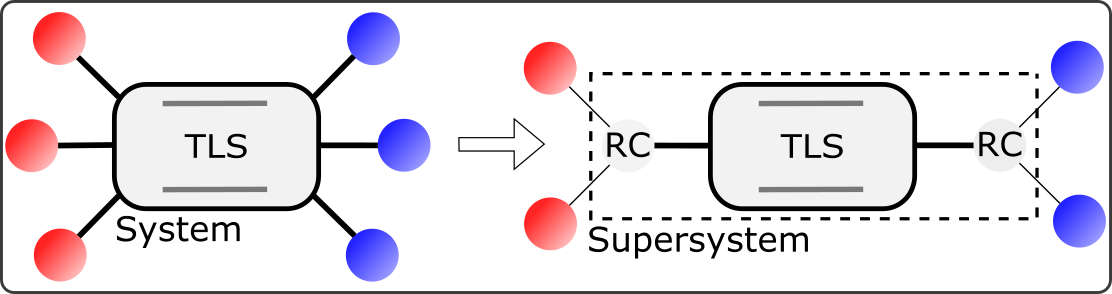
Figure 1: A two-level system interacting with two bosonic reservoirs held at different temperatures is mapped to an enlarged supersystem comprising the original two-level system coupled to two collective modes (one for each reservoir), which are in turn coupled to residual heat baths.

II Model: Derivation of the effective spin-boson Hamiltonian

We begin with the nonequilibrium spin-boson model allowing for strong coupling between the quantum system (spin) and the baths, which are characterized by peaked, Brownian oscillator spectral functions. After a series of transformations and truncations, the model is reduced into an effective SB model, which now can be assumed to be weakly coupled to the baths—described by modified spectral functions. The energy spacing of the effective spin and its coupling parameters to the baths are renormalized, thus providing understanding on the role of strong couplings in thermal transport.

II.1 The standard SB model

We start with a two-level system coupled to two heat baths ($i=h,c$) comprising collections of harmonic oscillators ($\hbar=1$, $k_{B}=1$),

$$H_{SSB} = \frac{\epsilon}{2}\sigma_{z}+\frac{\Delta}{2}\sigma_{x}+\sigma_{z}\sum_{k,i\in{\{h,c\}}}f_{k,i}(c_{k,i}^{\dagger}+c_{k,i})$$ (1)

$$+ \sum_{k,i\in{\{h,c\}}}\nu_{k,i}c_{k,i}^{\dagger}c_{k,i}.$$

Here, $\epsilon$ is the energy splitting of the spin, $\Delta$ is the tunneling frequency, $\sigma_{x,y,z}$ are the Pauli matrices, $c_{k,i}^{\dagger}$ ($c_{k,i}$) are the bosonic creation (annihilation) operators for the hot and cold baths ($i=h,c$) for a mode of frequency $\nu_{k,i}$. The displacements of the harmonic oscillators are coupled to the spin polarization with strength $f_{k,i}$, and these interactions are captured by the spectral density functions, $J_{SSB,i}(\omega)=\sum_{k}f_{k,i}^{2}\delta(\omega-\nu_{k,i})$. In what follows, we refer to the model Hamiltonian Eq. (1) as the “standard spin-boson model” (SSB).

Technically, it is convenient to first specify the spectral function of the residual baths, after the RC mapping (as we do in Sec. II.2), then work our way back and derive the spectral function of the SSB model. For completeness, we already present here the spectral function of the SSB model: It can be shown that an Ohmic function in the RC representation corresponds to a Brownian-oscillator model for the SSB model,

$$J_{SSB,i}(\omega)=\frac{4\gamma_{i}\omega\Omega_{i}^{2}\lambda_{i}^{2}}{(\Omega_{i}^{2}-\omega^{2})^{2}+(2\pi\gamma_{i}\Omega_{i}\omega)^{2}}.$$ (2)

We elaborate on this mapping in Appendix A. The physical picture emerging from this spectral function is that, in each bath, there is a collection of modes with frequencies centered around $\Omega_{i}$ that are strongly coupled to the system. The energy parameter $\lambda_{i}$ quantifies the coupling strength of the spin to the $i$th bath. The combination $\gamma_{i}\Omega_{i}$, with $\gamma_{i}$ a dimensionless parameter, provides a measure for the width of the spectral function. Since bath modes around $\Omega_{i}$ dominate the Brownian spectral function, by extracting an oscillator around this frequency from the $i$th bath, and including it into the system, we can capture strong system-bath coupling effects.

In simulations below, we work with the following range of parameters: $\Delta=1$, $\epsilon=0$ (for simplicity), $\Omega>\Delta$, small width for the spectral function $\gamma\ll 1$, and variable system-bath coupling strength $\lambda/\Delta$.

II.2 Reaction Coordinate mapping

We follow a procedure analogous to that described in Ref. (NazirPRA14, ), but extended here to the case of a system strongly coupled to two heat baths. In brief, we apply a normal-mode transformation to the harmonic part of Eq. (1) and define a collective coordinate for each environment, termed reaction coordinate. The two RCs ($i=h,c$) are each coupled directly to the spin, as well as to their residual harmonic bath. This mapping is sketched in Fig. 1. The resulting reaction coordinate (RC) Hamiltonian is given by

$$H_{RC} = \frac{\epsilon}{2}\sigma_{z}+\frac{\Delta}{2}\sigma_{x}+\sum_{i}\Omega_{i}a_{i}^{\dagger}a_{i}+\sigma_{z}\sum_{i}\lambda_{i}(a_{i}^{\dagger}+a_{i})$$ (3)

$$+ \sum_{k,i}\omega_{k,i}b_{k,i}^{\dagger}b_{k,i}+\sum_{i}(a_{i}^{\dagger}+a_{i})\sum_{k}g_{k,i}(b_{k,i}^{\dagger}+b_{k,i})$$

$$+ \sum_{i}(a_{i}^{\dagger}+a_{i})^{2}\sum_{k}\frac{g^{2}_{k,i}}{\omega_{k,i}}.$$

The two collective coordinates are defined such that,

$$\lambda_{i}(a_{i}^{\dagger}+a_{i})=\sum_{k}f_{k,i}\left(c_{k,i}^{\dagger}+c_{k,i}\right).$$ (4)

Here, $\lambda_{i}$ is the newly-defined coupling of each RC to the spin system, $\Omega_{i}$ are the corresponding frequencies of the reaction coordinates. The residual baths are denoted by creation (annihilation) operators $b_{k,i}^{\dagger}$ ($b_{k,i}$), which now couple only to the $i$th RC. The spectral density functions of the residual heat baths are defined as $J_{RC,i}(\omega)=\sum_{k}g_{k,i}^{2}\delta(\omega-\omega_{k,i})$.

It is important to note that this mapping is exact. To complete the mapping, the spectral density functions of the SSB and the RC models need to be coordinated such that the spin system follows a corresponding dynamics. For simplicity, we assume that the spectral functions of the residual baths are Ohmic,

$$J_{RC,i}(\omega)=\gamma_{i}\omega e^{-\omega/\Lambda_{i}}.$$ (5)

Here, $\gamma_{i}$ is a dimensionless coupling parameter of the RC to the residual bath. This parameter is assumed to be small in our simulations allowing us to use the second-order QME for the model after the RC mapping. $\Lambda_{i}$ is the cutoff frequency of the bath.

The reaction coordinate Hamiltonian, Eq. (3), comprises the following components: The enlarged system (supersystem), now including the original spin, two additional harmonic oscillators as the RCs, and the coupling of the spin to these two oscillators. Other terms in Eq. (3), appearing in the second line are the two residual heat baths ($i=h,c$) and their couplings to the two reaction coordinates. The last element (third line) is a nontrivial quadratic term, $\sum_{i}\left(a_{i}^{\dagger}+a_{i}\right)^{2}\sum_{k}\frac{g_{k,i}^{2}}{\omega_{k,i}}$. In Ref. NazirPRA14 it was treated as part of the interaction Hamiltonian and shown to be partially eliminated from the Markovian quantum master equation. In Ref. Correa19 , the exactly solvable model of a chain of harmonic oscillators coupled to harmonic baths was treated with the Langevin Equation, then compared to the approximate Lindblad method. It was pointed out that standard QME methods (such as in Lindblad form or Redfield) have to be executed without the quadratic term.

Essentially, an exact quantum equation of motion for the Hamiltonian (3) is reduced to a Markovian QME in which the bare parameters of the RC and its coupling to the system and bath ($\Omega$, $\lambda$, $g_{k,i}$) are to be used, rather than renormalized parameters defined once the quadratic term is absorbed YanRev . In Appendix B we perform a rotation transformation and absorb the quadratic term, by renormalizing the parameters of the reaction coordinate Hamiltonian. However, as pointed out in Refs. YanRev ; NazirPRA14 ; Correa19 , Markovian QME simulations in this rotated basis do not correspond to the original Hamiltonian.

II.3 Truncation of the RC Hamiltonian

Simulations of the RC model, Eq. (3) are performed by truncating it to include only $M$ equi-distant levels. We count these levels using an index $l$,

$$\Omega a^{\dagger}a \xrightarrow[]{} \sum_{l=0}^{M-1}\Omega\left(l+\frac{1}{2}\right)|l\rangle\langle l|,\,\,$$

$$\left(a^{\dagger}+a\right) \xrightarrow[]{} \sum_{l=1}^{M-1}\sqrt{l}\left(|l\rangle\langle l-1|+|l-1\rangle\langle l|\right).$$ (6)

For simplicity, we include the same number of states for each truncated RC. After the truncation, the Hamiltonian describes an enlarged system (ES) with a spin coupled to two $M$-level manifolds, with each $M$ manifold coupled to a residual heat bath,

$$H_{RC}^{M}=H_{ES}^{M}+H_{B}+H_{ES,B}^{M}.$$ (7)

Explicitly, the enlarged system Hamiltonian is

$$H_{ES}^{M} = \frac{\epsilon}{2}\sigma_{z}+\frac{\Delta}{2}\sigma_{x}+\sum_{i=h,c}\sum_{l_{i}=0}^{M-1}\Omega_{i}\left(l_{i}+\frac{1}{2}\right)|l_{i}\rangle\langle l_{i}|$$ (8)

$$+ \sigma_{z}\sum_{i=h,c}\lambda_{i}\sum_{l_{i}=1}^{M-1}\sqrt{l_{i}}|l_{i}\rangle\langle l_{i}-1|+h.c.$$

As before, the residual baths are given as a collection of harmonic oscillators, $H_{B}=\sum_{k,i}\omega_{k,i}b_{k,i}^{\dagger}b_{k,i}$. The extended system interacts with the two heat baths ($h,c$),

$$H_{ES,B}^{M}=\sum_{i=h,c}V_{ES,i}^{M}\otimes B_{i},$$ (9)

where we identify the system operator $V_{ES,i}^{M}$ and the coupled bath operator $B_{i}$ as

$$V_{ES,i}^{M} = \sum_{l_{i}=1}^{M-1}\sqrt{l_{i}}\left(|l_{i}\rangle\langle l_{i}-1|+|l_{i}-1\rangle\langle l_{i}|\right),$$

$$B_{i} = \sum_{k}g_{k,i}\left(b_{k,i}^{\dagger}+b_{k,i}\right).$$ (10)

The Hamiltonian $H_{ES}^{M}$ and system’s operators $V_{ES,i}^{M}$ are matrices of dimension $2M^{2}\times 2M^{2}$.

II.4 Diagonalization and the effective spin-boson model

As a quick review, we started from the SSB model in Sec. II.1. We extracted RCs, one from each bath in Sec. II.2 and we truncated the RCs in Sec. II.3. The last two steps of the procedure are described in this Section. They involve: (i) Diagonalizing the $M$-level RC extended-system $H_{ES}^{M}$ of Eq. (8). (ii) Truncating the resulting spectrum, leaving only two states—thus strikingly, finishing where we started with a two state system coupled to harmonic oscillator heat baths. Albeit, as we show next, the spin-boson model at the end of the procedure relates to the SSB model through renormalized parameters. In more details:

We diagonalize $H_{ES}^{M}$ of Eq. (8) with a unitary transformation $U$. In general, this procedure is done numerically. This transformation is further applied onto the interaction Hamiltonians in Eq. (10),

$$H_{ES}^{D}=U^{\dagger}H_{ES}^{M}U,\,\,\,\,\ V_{ES,i}^{D}=U^{\dagger}V_{ES,i}^{M}U.$$ (11)

As an example, in Fig. 2 we present the evolution of the eigenenergies $E_{n}$ of $H_{ES}^{M}$ with the coupling energy, $\lambda$. For simplicity, we use RCs with $M=2$, that is, the model includes a central spin and two two-level RCs. Overall, there are eight (many-body) occupation-basis states. For simplicity, the model is made to be fully symmetric; $\lambda=\lambda_{i}$ and $\Omega=\Omega_{i}$.

Since we work with $\Omega>\lambda$ and $\Omega\gg\Delta$, the global eigenstates of $H_{ES}^{M}$ can be associated with the local picture of a central spin and two (left and right) RC oscillators. The lowest two eigenstates in Fig. 2(b), are separated by $\approx\Delta$. They correspond to the two RCs residing in their respective ground states (energy $2\times\frac{1}{2}\Omega$), while the central spin occupies either its ground or excited states. Higher eigenenergies in Fig. 2(a) correspond to excited RCs, and are separated by multiples of $\Omega$. Specifically, there are four levels clustered around $2\Omega$ corresponding to one RC in its ground state and the other in its first excited state, with the spin occupying its ground or excited state. The top two levels in Fig. 2 are associated with both RCs being excited, and the spin occupying its ground or excited state. One can similarly explain level structure for $M>2$.

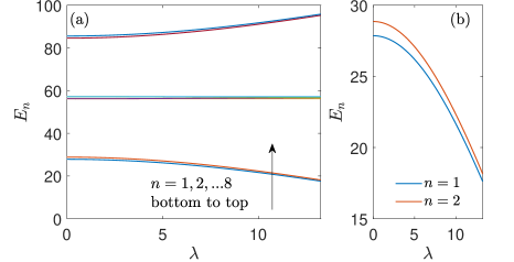
Figure 2: (a) Eigenenergies of $H_{ES}^{M=2}$ with $\Delta=1$, $\epsilon=0$, $\Omega=28\Delta$ commentP . (b) Focus on the lowest two eigenvalues, which form an effective spin Hamiltonian.

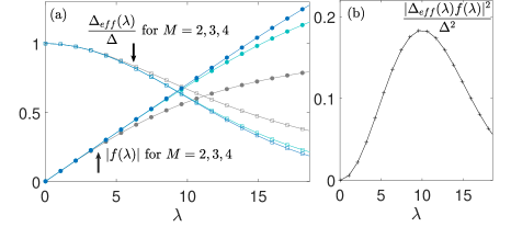
Figure 3: Behavior of the renormalized parameters in the effective spin-boson model, Eq. (12). (a) The spin splitting $\Delta_{eff}(\lambda)$ and the coupling function $f(\lambda)$ are obtained numerically from the diagonalization transformation of $H_{ES}^{M}$. (b) We present the combination $[\Delta_{eff}(\lambda)f(\lambda)]^{2}$, which controls the heat current for ohmic spectral functions at weak coupling. $\epsilon$ = $0$, $\Omega$ = $28\Delta$.

We now discuss our choice of parameters. In previous studies e.g. in Ref. NazirPRA14 , the parameters of the RC model Eq. (3) were such that $\Omega\sim\Delta$, and $\Omega\sim T$. Here, with the objective to uncover the role of strong couplings, we use a high frequency RC mode, $\Omega\gg\Delta$ and $\Omega\gg T$ such that we can safely truncate the spectrum of each RC and include few levels when performing heat transport calculations. This choice of parameters allows us to focus on the strong-coupling limit while bypassing issues of convergence involved in the truncation of the harmonic oscillator manifold. As a result of this truncation, we are able to construct an effective model, which exposes the essence of strong interactions, and is highly accurate as we show in section IV. In Appendix D we include additional simulations of the heat current at strong coupling using smaller values of $\Omega$, down to $\Omega=5\Delta$.

Inspecting Fig. 2, we make a useful observation: Since in simulations we work with $T\ll\Omega$, excited states beyond the first two levels are thermally inaccessible as there is a dramatic energy separation between the first two levels (gapped by $\leavevmode\nobreak\ \Delta$), and the rest of the eigenenergy manifold. Based on this observation, we truncate the spectrum of $H_{ES}^{D}$ and write down an effective spin-boson Hamiltonian,

$$H_{SB}^{eff} = \frac{1}{2}\Delta_{eff}(\vec{\lambda})\sigma_{z}+\sigma_{x}\sum_{i}f_{i}(\vec{\lambda})\sum_{k}g_{k,i}(b_{k,i}^{\dagger}+b_{k,i})$$ (12)

$$+ \sum_{k,i}\omega_{k,i}b_{k,i}^{\dagger}b_{k,i},$$

with

$$\Delta_{eff}(\vec{\lambda})=E_{2}(\vec{\lambda})-E_{1}(\vec{\lambda}),\,\,\,\,\,f_{i}(\vec{\lambda})=\langle 1(\vec{\lambda})|V_{ES,i}^{D}|2(\vec{\lambda})\rangle.$$

We denote the pair $\lambda_{i}$ with a vector notation, ${\vec{\lambda}}=(\lambda_{h},\lambda_{c})$. $E_{n}(\vec{\lambda})$ are the eigenvalues of $H_{ES}^{D}$ with eigenstates $|n(\vec{\lambda})\rangle$; $n=1,2$, as depicted e.g. in Fig. 2. We refer to the Hamiltonian (12) as the “effective spin-boson (EFF-SB) model”.

We highlight the dependence of the spin splitting on the interaction energies $\vec{\lambda}$. The dimensionless function $f_{i}(\vec{\lambda})$ arises from the transformation of the enlarged system Hamiltonian into the diagonal basis and it describes the dressing of the system-bath coupling energies. It depends on both coupling energies, $\lambda_{h}$ and $\lambda_{c}$ and this fact immediately suggests that cooperative, two-bath interactions should play a role in the dynamics and steady state transport behavior, as indeed is the case based on the polaronic approach PRL05 ; QME06 ; NIBA11 ; NIBA14 .

To understand the impact of strong system-bath couplings, we depict in Fig. 3 the effective spin splitting and the coupling function $f_{i}(\vec{\lambda})$. Since henceforth we use equal couplings (until Sec. V), we relieve the vector notation, and identify by $\lambda$ the (equal) couplings of the spin to both reservoirs. On the one hand, strong coupling effects should facilitate transport by enhancing the coupling of the spin to the baths. Indeed, $f(\lambda)$ is an increasing function of $\lambda$. On the other hand, the detrimental impact of strong coupling clearly emerges through the suppression of $\Delta_{eff}(\lambda)$, the tunneling splitting between the levels of the effective spin. Roughly, as we reduce the spin splitting, less energy is transmitted per quanta transferred. In Appendix C we present analytical derivations on a simpler model to support the observed suppression of $\Delta_{eff}$ with $\lambda$. When focusing on quantum dynamics, the suppression of $\Delta_{eff}(\lambda)$ would eventually lead to the localization of the spin Weiss . In calculations of steady state heat transport as we perform here, the substantial suppression of $\Delta_{eff}(\lambda)$ shows up in the rapid decline of the heat current at strong coupling.

We fit the functions in Figure 3(a) and find that, approximately, $\Delta_{eff}(\lambda)\propto\exp\left(-\frac{\lambda^{2}}{\lambda_{m}^{2}}\right)$ and $f(\lambda)\propto\lambda$, with $\lambda_{m}$ a parameter with the dimension of energy. Importantly, since $f(\lambda)$ is of order 1, as long as $\gamma\ll 1$ [see Eq. (5)], we can still safely employ a weak coupling scheme to treat the dynamics and transport characteristics of the effective-SB Hamiltonian Eq. (12).

We present the combination $[\Delta_{eff}(\lambda)f(\lambda)]^{2}$ in Fig. 3(b) and reveal a non-monotonic behavior: The product first grows approximately as $\lambda^{2}$ then it decays rapidly as $\exp(-\lambda^{2}/\lambda_{m}^{2})$, with a maximum at $\lambda_{m}/\sqrt{2}$. As we discuss in more details in Sec. IV, the steady state heat current in the SB model is proportional to this product for Ohmic baths under the weak system-bath coupling approximation PRL05 ; QME06 ; NIBA14 ; ARPC . Thus, the trend observed in Fig. 3(b) is representative of the heat current in this regime.

While the condition of weak system-bath coupling does not hold for the SSB model since $\lambda/\Delta$ can be large, it is valid for the effective SB model since its coupling to the bath is dictated by the width parameter ${\gamma}_{i}$, which is assumed small. This is the main physical and computational outcome of the mapping approach: The effective spin-boson model captures strong coupling effects, as inherited from the SSB model, but now embedded in renormalized parameters while allowing a weak coupling treatment to the baths.

The effective SB model described in this subsection is highly beneficial as it hands over analytic understanding on transport characteristics. It is important to appreciate that the EFF-SB model should be identified only after constructing a RC that converges with respect to $M$, the number of levels representing the RC. This aspect is clearly manifested in Fig. 3. While $\Delta_{eff}(\lambda)$ and $f(\lambda)$ readily converge with $M$ at weak-intermediate couplings, at strong coupling increasingly more levels should be included to converge the parameters of the effective SB model.

III Method: steady state energy transport with the RC-QME

We succeeded in transforming the SSB model with possibly strong coupling of the spin to harmonic oscillator baths into an effective SB model. The parameter $\gamma\Omega$ in the SSB model, which controls the width of the spectral function, dictates the system-bath coupling energy in the RC picture. Thus, if we assume a narrow spectral function for the SSB model, in the RC model the extended system becomes weakly coupled to its surroundings. As a result, the dynamics and steady state characteristics of the effective SB can be studied using a QME perturbative in the system-bath coupling.

Here, we employ the Markovian Redfield master equation to study the steady state behavior under the Hamiltonian (7)-(10). This approach relies on three assumptions: (i) The enlarged system is weakly coupled to its residual environments such that a second-order perturbative approach yields proper results. (ii) The residual environments act as Markovian baths. (iii) The initial state of the total system factorizes into a system times bath form. The residual thermal baths are individually prepared in their canonical states characterized by inverse temperatures $\beta_{i}$.

Working in the Schrödinger picture and in the energy basis of the subsystem, the Redfield equation for the reduced density matrix of the enlarged system (dimension $2M^{2}$) is given by Nitzan ; Breuer ,

$$\dot{\rho}_{ES,mn}(t) = -i\omega_{mn}\rho_{ES,mn}(t)$$ (14)

$$+ \sum_{i}\sum_{j,k}[R_{mj,jk}^{i}(\omega_{kj})\rho_{ES,kn}(t)+R_{nk,kj}^{i*}(\omega_{jk})\rho_{ES,mj}(t)$$

$$- R_{kn,mj}^{i}(\omega_{jm})\rho_{ES,jk}(t)-R_{jn,mk}^{i*}(\omega_{kn})\rho_{ES,jk}(t)].$$

Here, $\omega_{mn}=E_{m}-E_{n}$ are the bohr frequencies of the enlarged system in the energy basis. The $R$ super-operator terms in Eq. (14) are given by half Fourier transform of bath autocorrelation functions,

$$R_{mn,jk}^{i}(\omega) = (V_{ES,i}^{D})_{m,n}(V_{ES,i}^{D})_{j,k}\int_{0}^{\infty}d\tau e^{i\omega\tau}\langle B_{i}(\tau)B_{i}\rangle$$ (15)

$$= (V_{ES,i}^{D})_{m,n}(V_{ES,i}^{D})_{j,k}[\Gamma_{RC,i}(\omega)+i\Delta_{RC,i}(\omega)].$$

The autocorrelation functions of bath operators are evaluated with respect to the thermal state of their respective baths. In what follows, we neglect the imaginary component of the dissipators, $\Delta_{RC}$, as it can be shown that they cancel out the quadratic term in the RC Hamiltonian, Eq.(3) NazirPRA14 .

For harmonic environments and a bilinear coupling between the enlarged system and the residual environments, the real part of the $R$ term reduces to

$$\Gamma_{RC,i}(\omega)=\begin{cases}\pi J_{RC,i}(\omega)n_{i}(\omega)&\omega>0\\ \pi J_{RC,i}(|\omega|)[(n_{i}(|\omega|)+1]&\omega<0.\end{cases}$$ (16)

Here, $n_{i}(\omega)$ is the Bose-Einstein distribution function of the $i$th bath; $J_{RC,i}(\omega)$ is the RC spectral function given by Eq. (5).

To calculate the heat current flowing through the system, we write down the Redfield equation as

$$\dot{\rho}_{ES}(t)=-i[H_{ES}^{D},\rho_{ES}]+D_{h}(\rho_{ES})+D_{c}(\rho_{ES}),$$ (17)

with the dissipators $D_{h,c}(\rho_{ES})$ organized based on Eq. (14). The dissipators are additive given the weak coupling of the RCs to their residual baths (but each dissipator $D_{i}$ depends non-additively on the original coupling parameters, $\lambda_{i}$).

We solve the equation of motion in steady state, $\dot{\rho}_{ES}(t)=0$ and obtain the density matrix of the enlarged system, $\rho_{ES}^{ss}$. The steady state heat current at the $i$th bath, calculated from the heat exchange between the enlarged system and this reservoir is given by

$$J_{i}={\rm Tr}\left[D_{i}(\rho_{ES}^{ss})H_{ES}^{D}\right].$$ (18)

The heat current is defined positive when flowing from the $i$th bath towards the system. This procedure, the application of the Redfield-QME onto the RC model is referred to as the reaction-coordinate quantum master equation method, RC-QME.

Below, we perform heat transport simulations of the nonequilibrium spin-boson model using four methods:

(i) RC-QME framework: We follow the approach described in this Section, while checking convergence by increasing $M$, the number of levels used to describe the RCs.

(ii) Weak coupling, BMR-QME calculations: We calculate the heat current with the original SSB Hamiltonian Eq. (1) without performing the RC mapping under the (unjustified) weak coupling assumption, so as to highlight signatures of strong-couplings. In this case, we again employ the Redfield Equation Eq. (14) in the diagonal representation but use $J_{RC}(\omega)\xrightarrow{}J_{SSB}(\omega)$. Obviously, this calculation (based on an analytic expression PRL05 ; QME06 ; NIBA14 ; ARPC ) is appropriate only when the coupling of the spin to the baths is weak.

(iii) PT-NEGF: We use the polaron-transformed NEGF method developed in Ref. PT-NEGF17 , denoted by “PT-NEGF”. This method, tested on the nonequilibrium spin-boson model, is capable of treating nonperturbatively the system-bath coupling term. It also handles the tunneling energy in a perturbative manner. The method combines the polaron transformation with the nonequilibrium Green’s function method, where a Majorana-fermion representation is utilized to evaluate the Dyson series.

(iv) EFF-SB model: We obtain the parameters of the effective two-state model based on the diagonalization of $H_{ES}^{M}$ with large enough $M$. However, since we end up with two states weakly coupled to the surroundings, we can utilize the closed-form expression for the heat current as derived in Refs. PRL05 ; QME06 , assuming a Markovian, Ohmic bath. We write down this expression emphasizing the nontrivial dependence of parameters on the renormalized spin splitting,

$$J_{q}^{eff}=\Delta_{eff}\frac{J_{RC,h}^{eff}(\Delta_{eff})J^{eff}_{RC,c}(\Delta_{eff})\left[n_{h}(\Delta_{eff})-n_{c}(\Delta_{eff})\right]}{J^{eff}_{RC,h}(\Delta_{eff})\left[2n_{h}(\Delta_{eff})+1\right]+J^{eff}_{RC,c}(\Delta_{eff})\left[2n_{c}(\Delta_{eff})+1\right]}.$$ (19)

The Ohmic spectral function, which is evaluated at the renormalized splitting, is dressed by $f(\lambda)$. For brevity, we suppress the dependence of $\Delta_{eff}$ on $\lambda$,

$$J^{eff}_{RC}(\Delta_{eff})=\gamma\Delta_{eff}|f(\lambda)|^{2}e^{-\Delta_{eff}/\Lambda}.$$ (20)

For a symmetric system in the limit of high $\Lambda$ the heat current reduces to

$$J_{q}^{eff}=\gamma|f(\lambda)|^{2}[\Delta_{eff}(\lambda)]^{2}\frac{n_{h}(\Delta_{eff})-n_{c}(\Delta_{eff})}{2n_{h}(\Delta_{eff})+2n_{c}(\Delta_{eff})+2}.$$

(21)

In Fig. 3(b) we showed that the temperature-independent prefactor of this function displayed a turnover behavior with $\lambda$,

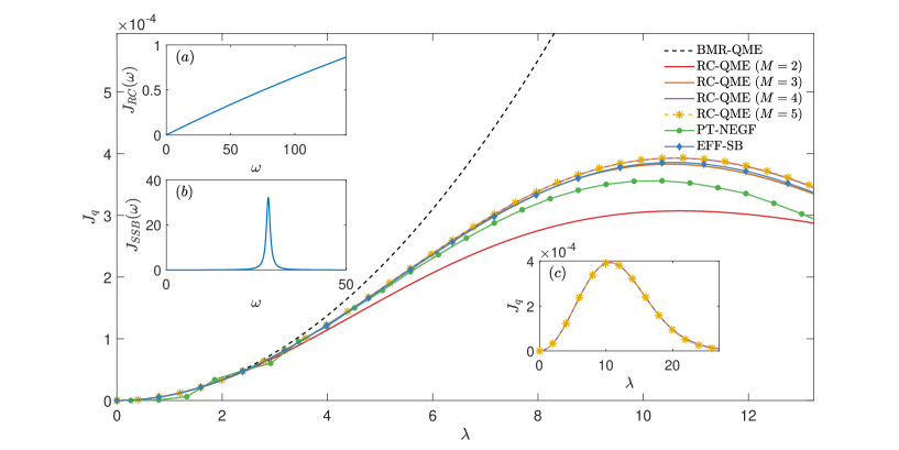
Figure 4: Steady state heat current as a function of coupling strength $\lambda$. We compare RC-QME simulations ($M=2-5$) to BMR-QME (dashed) and PT-NEGF ($\circ$) results. RC-QME simulations with $M=4-5$ overlap. We further display the current predicted from the effective SB model (EFF-SB), Eq. (19). (a)-(b) Spectral density functions of the reaction coordinate model and the standard spin-boson model, respectively. Parameters are $\epsilon$ = $0$, $\Omega$ = $28\Delta$, $\gamma$ = $0.0071/\pi$ and $\Lambda=1000\pi\Delta$. The temperatures are $T_{h}$ = $\Delta$, $T_{c}$ = $0.5\Delta$. In panel (b), we employ $\lambda$ = $8\Delta$. (c) Demonstration of the full suppression of the heat current at strong coupling based on RC-QME simulations for $M=4$ and $M=5$ (overlapping).

IV Numerical Simulations

IV.1 System-bath coupling

We begin by studying the behavior of the heat current as a function of the system-bath coupling strength. In the SSB model of Sec. II.1, the parameter $\lambda_{i}$ quantifies the system-bath coupling, see Eq. (2). In the RC picture, this parameter describes the coupling of the spin to the added reaction coordinates, while the enlarged-system-bath coupling is controlled by $\gamma$.

Figure 4 depicts the steady state heat current as a function of $\lambda$ using our RC-QME framework. We further show the BMR-QME, EFF-SB, and the PT-NEGF results. For simplicity, we assume a symmetric setup, $\lambda=\lambda_{i}$, $\Omega=\Omega_{i}$, $\gamma=\gamma_{i}$, $\Lambda=\Lambda_{i}$.

We find that the heat current obtained from the BMR-QME grows quadratically with $\lambda$; recall that the spectral function scales as $J_{SSB}(\omega)\propto\lambda^{2}$. In contrast, the RC-QME depicts a turnover behavior, in a good agreement with the PT-NEGF method (which takes into account strong coupling effects through the Polaron transformation and the Dyson-series summation). Notably, the turnover behavior of the current with the coupling energy is excellently captured by the effective-SB model, Eq. (19) with the renormalized parameters, displayed in Fig. 3. Parameters for the effective model were taken using $M=4$.

Figure 5 shows the steady state heat current for a smaller value of $\Omega$. Recall, that this parameter controls the peak position and width of the SSB spectral density, Eq. (2). We again observe a very good agreement between strong coupling methods. Notably, we notice that the EFF-SB better agrees with the PT-NEGF technique than the RC-QME method at $M=4$. This trend is further exemplified in Appendix D, and discussed in details in Sec. IV.4.

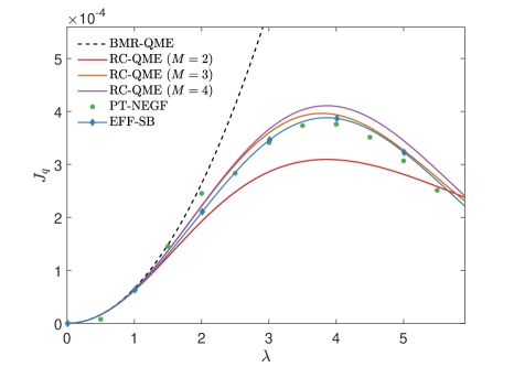
Figure 5: Steady state heat current as a function of coupling strength $\lambda$. Parameters are the same as in Fig. 4, except $\Omega=10\Delta$.

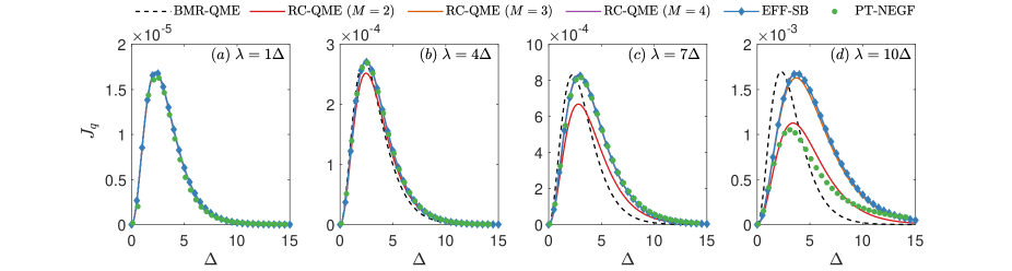
Figure 6: (a)-(d) Steady state heat current as a function of tunneling splitting from weak to strong couplings. Parameters are the same as in Fig. 4.

IV.2 Tunneling splitting

We study the behavior of the heat current as a function of the tunneling splitting $\Delta$ in Fig. 6, separately looking at weak (a), intermediate (b)-(c) and strong (d) system-bath couplings. The dependence of $J_{q}$ on the tunneling splitting was previously investigated analytically with NIBA NIBA11 and the BMR-QME Nazim14 , and numerically, with exact methods Segal13 ; Nazim14 ; PI . The general trend observed is of the heat current first growing with $\Delta$ quadratically. However, for larger spin splitting such that $\Delta>T$, $J_{q}$ begins to decay with $\Delta$. This suppression of the current can be rationalized in the weak coupling picture when only resonant processes contribute: When $\Delta$ becomes large, bath modes at this frequency are not thermally populated, resulting in the suppression of the heat current.

Inspecting Fig. 6, we find that the different methods agree at weak coupling. However, as we move into the intermediate and strong coupling regimes the current predicted by the BMR-QME offsets from the RC-QME. This is expected: We learned from Fig. 3 that strong coupling manifests itself in the renormalization (suppression) of the tunneling splitting. As such, in the BMR-QME method the position of the peak occurs at $\Delta\sim T$ while it appears only at a higher splitting for the RC-QME, once $\Delta_{eff}\sim T$. Interestingly, while the BMR-QME method incorrectly positions the peak, the maximal magnitude of the current is the same as in the RC-QME method.

As for the PT-NEGF method, while it agrees with the RC-QME at weak-intermediate couplings, see Fig. 6(a)-(c), more substantial deviations show up at strong coupling (up to 50%) and for large splitting, see Fig. 6(d). However, while the magnitude of the current differs between the RC-QME and the PT-NEGF methods, the peak position agrees. This manifests that the essential aspect of gap renormalization is captured in both methods, which is significant given the distinct ways they handle strong coupling effects. Which method, RC-QME or PT-NEGF is more accurate at strong coupling and large spin-splitting? We think that the RC-QME provides a more accurate result in this difficult regime: The PT-NEGF method does not handle exactly the spin splitting at large $\Delta$; while it is more accurate than the Markovian NIBA method of Ref. NIBA11 , which can only capture the $J_{q}\propto\Delta^{2}$ scaling, the self-energy in the PT-NEGF includes $\Delta$ only perturbatively. In contrast, the RC-QME handles both $\Delta$ and $\lambda$ non-perturbatively. Nevertheless, additional benchmarking is required to determine the exact behavior of the current at strong coupling and at large tunneling splitting.

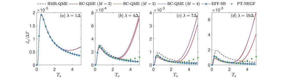
Figure 7: (a)-(d) Steady state heat current, divided by the temperature difference, as a function of the average temperature of the baths. Parameters are the same as in Fig. 4. We set $\Delta T=0.3T_{a}$, and $T_{h/c}=T_{a}\pm\Delta T/2$.

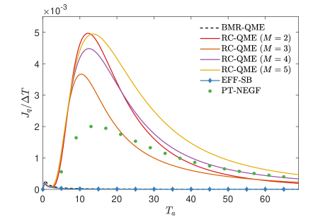
Figure 8: Steady state heat current divided by the temperature difference as a function of the averaged temperature of the reservoirs. This figure corresponds to Fig. 7 (c), but continuing here into the high temperature regime. Parameters are the same as in Fig. 4.

IV.3 Temperature-difference dependence

We study the behavior of the heat current as a function of the average temperature, $T_{a}\equiv(T_{h}+T_{c})/2$ in Figs. 7-8. Inspecting the low-intermediate temperature regime of $T_{a}<2\Delta$ in Fig. 7, we observe that the different methods display a crossover behavior: The current rises with $T_{a}$ as it approaches a resonance condition at $\Delta$ (or $\Delta_{eff}$ in the RC-QME). However, at higher temperatures the current drops as $1/T_{a}$ due to the temperature dependence of the scattering rates as captured by Eq. (19). The BMR-QME overestimates the current at strong couplings since it does not capture the suppression of $\Delta$, thus it allows for the transfer of more heat than in the RC-QME method.

As we raise the temperature, $T_{a}>2\Delta$, we observe in Fig. 7, and in more details in Fig. 8, a dramatic enhancement of the current, particularly at strong coupling. As a clue to deciphering the origin of this enhancement, we note that it is not captured by the EFF-SB model thus it emerges from the contributions of higher-energy transitions in the manifold of the extended system, see Fig. 2. Naturally, we question whether the enhancement of the current at high temperature is physical, or is it an artifact of the extraction of a single oscillator mode as a RC. However, in Fig. 8 we show that the PT-NEGF method also displays this enhancement, though there are differences in the magnitude of the current.

Altogether, as a function of temperature, we gather from Figs. 7 and 8 that the heat current is peaked first around $T_{a}\approx\Delta$ then at $T_{a}\approx\Omega$ (there are additional peaks at higher temperature). In the RC picture, we can explain this structure as follows: The current is high when $T_{a}$ roughly matches transition frequency in the extended system. The first peak corresponds to the excitation of the spin, with the RCs in their ground state. The second peak corresponds to energy transfer via the excitation of the RCs.

Interestingly, using the PT-NEGF method we can explain these peaks with a different picture, thinking about resonant and off-resonant (tunneling) transport of phonons. The first peak at $T_{a}\approx\Delta$ corresponds to resonant transmission of phonons from the bath through the spin. Beyond that at higher temperatures, the transport process occurs increasingly via tunneling: high frequency phonons from the baths must utilize the low frequency spin impurity to transfer heat. This off-resonant process becomes more potent as the temperature rises eventually matching the peak of the baths spectral density function (recall that we use a Brownian function in the SSB model), where the bath density of state is maximized. If one continues and increases the temperature, additional peaks will show up at multiples of $\Omega$. They would represent multi-phonon transfer processes in the PT-NEGF method, and the excitation of high energy levels in the extended-system RC model.

IV.4 Discussion: The exceptional performance of the effective Spin-boson model

The effective SB model brings insight on the strong coupling regime, and it allows fast computations. More surprisingly, as we show e.g. in Figs. 4-5 and Appendix D, it consistently provided results more accurate than those achieved with the full $2M^{2}$ model Hamiltonian, Eq. (7) as long as $T\ll\Omega$, $\Delta\ll\Omega$. What is the explanation for the remarkable success of the EFF-SB model? We can explain this superior behavior by noting that weak-coupling methods typically overestimate the heat current compared to exact results Nazim14 . In the RC-QME framework, as we include a large number of states for the RC ($M>2)$, many transitions contribute to the heat current, thereby increasing the error associated with the weak coupling scheme. Thus, while a large $M$ more accurately represents the RC oscillators, at the same time errors associated with the calculation of the current using a weak-coupling method become more significant.

In contrast, the effective SB model offers an excellent, fortunate tradeoff of these two aspects: On the one hand, it is constructed by diagonalizing a large $M$-RC Hamiltonian, Eq. (7); the renormalized parameters therefore capture the RC manifold. On the other hand, the subsequent truncation of the $2M^{2}$ spectrum, to include only few (two) states limit the over-estimation error associated with weak coupling schemes.

V Thermal-diode effect

The nonequilibrium spin-boson model was originally introduced to describe a quantum thermal diode (rectifier) PRL05 ; QME06 . In a boson-bath nanojunction, this effect relies on two conditions: anharmonicity, captured here by the impurity spin, and spatial asymmetry, introduced here by coupling the spin asymmetrically to the different baths. Recently, the nonequilibrium spin-boson model was realized in a superconducting quantum circuit demonstrating a diode effect with rectification ratio $R=|\frac{J_{q}(T_{h},T_{c})}{J_{q}(T_{c},T_{h})}|=1.1$ PekolaE . An important question that has been touched on, without conclusion is whether strong coupling effects are beneficial for the diode effect, and to what extent. The EFF-SB model offers computation at low cost, and we utilize it here to address this question.

The quantity of interest here is the thermal rectification ratio, $R$, which quantifies transport asymmetry when reversing the temperature bias. In this definition, $R=1$ corresponds to lack of rectification, while $R>1$, or $R<1$ corresponds to a diode effect. To materialize this effect, spatial symmetry needs to be introduced into the model. This is done here through the use of an asymmetry parameter $-1<\chi<1$, with $\lambda_{h}=\lambda(1-\chi)$, $\lambda_{c}=\lambda(1+\chi)$. In this definition, $\chi=0$ corresponds to the symmetric model where no rectification is expected.

Using Eq. 19, we obtain an analytic expression for the rectification ratio

$$R = \frac{\frac{f_{L}(\vec{\lambda})}{f_{R}(\vec{\lambda})}(2n_{c}(\Delta_{eff})+1)+(2n_{h}(\Delta_{eff})+1)}{\frac{f_{L}(\vec{\lambda})}{f_{R}(\vec{\lambda})}(2n_{h}(\Delta_{eff})+1)+(2n_{c}(\Delta_{eff})+1)}.$$ (22)

This equation reveals that the ratio of the effective coupling parameters breaks spatial symmetry in the system, allowing a diode effect to emerge. Indeed, if $f_{L}(\vec{\lambda})=f_{R}(\vec{\lambda})$, then $R=1$ and the system will not exhibit a diode behaviour.

Figure 9 examines the effect of asymmetry in the coupling strength on the diode effect. We test the effect at different coupling strengths $\lambda$ and for two temperature biases. First, in Fig. 9 (a) and (c) we display the heat current itself in the forward direction using the BMR-QME and the EFF-SB methods. Notably, the current is not maximal when the coupling is symmetric, rather, the current reaches an extremum when the qubit couples more strongly to the cold bath. Fig. 9(b) and (d) display the corresponding rectification ratios using the BMR-QME and the effective SB models. At stronger coupling the rectification ratio increases. However, this increase is rather minor. Identifying strategies for significantly enhancing the thermal diode effect in impurity models remain a challenge.

Figure 9: Thermal diode effect at strong coupling with the EFF-SB model (filled and empty $\diamond$) and the weak coupling BMR-QME (full and dashed lines) at $\Delta T=0.5\Delta$ and $\Delta T=1\Delta$. Panels (a) and (c) depict the steady state heat current as a function of the asymmetry parameter $-1<\chi<1$, $\lambda_{h}=\lambda(1-\chi)$, $\lambda_{c}=\lambda(1+\chi)$. Panels (b) and (d) depict the associated rectification ratios $R$. Parameters are the same as in figure 4.

VI Summary

We presented the reaction coordinate framework, RC-QME for studies of quantum heat transport in nanoscale systems beyond the weak system-bath coupling limit. In this method, degrees of freedom of the baths, which are strongly coupled to the system are extracted and explicitly included into the system. After performing additional, physically-motivated transformations and truncation, transport characteristics of the enlarged system are computed using a perturbative, Markovian QME method. The main results of our work are:

(i) On the fundamental side, by continuing with physically-motivated transformations of the RC Hamiltonian we ended up with a spin-boson model, albeit with renormalized parameters. The effective SB model elegantly reveals the impact of strong system-bath coupling on spin dynamics and heat transport behavior, by manifesting competing effects: When increasing the system-bath coupling energy the effective spin splitting is strongly reduced. On the other hand, the coupling of the effective spin to the baths increased approximately linearly. One could generalize the principles behind the effective SB model, construct other effective few-level models with energy parameters renormalized to absorb strong coupling effects, and describe the operation of more complex thermal machines.

(ii) On the application side, by comparing our method to another scheme that utilizes the polaron transformation, we can safely conclude that our method captures system-bath coupling effects beyond low order perturbation theory treatments. Specifically, the RC-QME method reproduced the turnover behavior of the heat current with $\lambda$, the system-bath interaction parameter, in a quantitative agreement with the polaron-NEGF method. Furthermore, we demonstrated that the RC-QME method took into account off-resonant phonon transmission processes. This was manifested in the behavior of the heat current with temperature: The current showed multiple peaks representing resonant, then enhanced off-resonant transport once the temperature matched the peak of the bath density of states (spectral function). We further looked at the diode behavior of the asymmetric SB model and showed that strong coupling effects could enhance the rectification behavior, albeit to a small extent.

The construction of an effective SB model is one of the central results of this work, allowing us to rationalize strong coupling effects, as well as perform calculations at minimal computational cost. Once reaching the effective SB model, quantum dynamics and transport behavior can be evaluated with a perturbative QME method, as we did here. Moreover, one can further employ the effective SB model in conjunction with more accurate techniques developed for the SB model, such as the NIBA NIBA11 and Majorana-fermion NEGF methods NJP17 ; PT-NEGF17 . Even more so, once reaching the effective-SB model one could continue iteratively with the RC transformation, to extract additional modes into the system (transforming the spectral function numerically). As such, this technique is not limited to spectral functions that are peaked around a central mode. Our method differs from chain mapping techniques such as TEPODA Plenio1 ; Plenio2 ; Plenio3 , since we are able to study the strong coupling regime semi-analytically, gaining physical intuition and minimizing computational costs.

The RC-QME method described in this paper should be extended in two ways: First, one should test whether it is still accurate in models where the spectral density function of the SSB is not peaked at a single frequency as in the Brownian oscillator model, but rather resembles e.g. an Ohmic model. In such cases, one should find how many oscillators should be extracted from the baths to capture quantitatively strong coupling effects, and how does the reaction coordinate method correspond to the polaron model. Second, the RC method and the effective Hamiltonian principle can be feasibly generalized to describe the coupling of multi-level quantum systems to multiple reservoirs. As such, it is suitable to study the operation of strongly-coupled quantum heat machines, our objective in future studies.

Appendix A Reaction coordinate mapping

The reaction coordinate mapping would be incomplete without addressing how the SSB and the RC spectral density functions are related to each other. We find this correspondence by studying the dynamics of the system in the two representations. To generalize the discussion, we consider a coordinate $q$ moving in a confining potential $U(q)$. We will make use of classical equations of motions but an analogous treatment can be done quantum mechanically. This can be done because the spectral density function only contains information about the harmonic baths and their interaction with the system, which is linear in the oscillators’ displacements. Our discussion here follows Ref. NazirPRA14 . It is included here for completeness, demonstrating its generalization for the case of a system coupled to two heat baths.

Starting from the SSB Hamiltonian Eq. (1), the classical analogue of the SSB model takes the form

$$H_{q} = \frac{P_{q}^{2}}{2}+U(q)+q\sum_{k,i}\phi_{k,i}x_{k,i}+q^{2}\sum_{k,i}\frac{\phi_{k,i}^{2}}{2\nu_{k,i}^{2}}$$ (A1)

$$+ \frac{1}{2}\sum_{k,i}(p_{k,i}^{2}+\nu_{k,i}^{2}x_{k,i}^{2}).$$

Here, we introduce the compact form $\phi_{k,i}\equiv\sqrt{2\nu_{k,i}}f_{k,i}$. Also, we identify the position and momenta of the environment as:

$$x_{k,i}=\sqrt{\frac{1}{2\nu_{k,i}}}(c_{k,i}^{\dagger}+c_{k,i})$$ (A2)

and

$$p_{k,i}=i\sqrt{\frac{\nu_{k,i}}{2}}(c_{k,i}^{\dagger}-c_{k,i}).$$ (A3)

Using this Hamiltonian, we obtain the classical equations of motion for the coordinate $q$ and each bath mode $x_{k,i}$:

$$\ddot{q}(t) =-U^{\prime}(q)-\sum_{k,i}{\phi}_{k,i}x_{k,i}(t)-q(t)\sum_{k,i}\frac{{\phi}^{2}_{k,i}}{\nu_{k,i}^{2}},$$ (A4)

$$\ddot{x}_{k,i}(t) =-q(t){\phi}_{k,i}-\nu_{k,i}^{2}x_{k,i}(t).$$ (A5)

Here, $U^{\prime}(q)$ corresponds to a derivative with respect to the coordinate $q$. Working in Fourier space, where observables take the form $\check{q}(z)=\int_{-\infty}^{\infty}dte^{-izt}q(t)$, it is possible to eliminate the environment variables from the equations of motion. Doing so, we obtain an algebraic equation $K(z)\check{q}(z)=-\check{U^{\prime}}(z)$. Here, the Fourier space kernel $K(z)$ is defined as:

$$K(z) = -z^{2}\left(1+\sum_{k,i}\frac{{\phi}_{k,i}^{2}}{\nu_{k,i}^{2}(\nu_{k,i}^{2}-z^{2})}\right)$$ (A6)

$$= -z^{2}\left(1+2\sum_{i}\int_{0}^{\infty}d\nu\frac{J_{SSB,i}(\nu)}{\nu(\nu^{2}-z^{2})}\right)$$

$$= -z^{2}\left(1+\sum_{i}\int_{-\infty}^{\infty}d\nu\frac{J_{SSB,i}(\nu)}{\nu(\nu^{2}-z^{2})}\right).$$

The integral can be solved by the residue theorem making use of the simple pole at $\nu=z$. thus, the kernel takes the form:

$$K(z)=-z^{2}+\pi i\sum_{i}J_{SSB,i}(z).$$ (A7)

At this stage, we repeat the same procedure after the RC transformation, and identify the kernel $K(z)$ in terms of the RC spectral densities. Since the mapping is exact, the two kernel functions, before and after the normal mode transformation, should be identical. Following a similar procedure as before, we replace the Hamiltonian Eq. (3) by a classical coordinate moving in a potential $U(q)$. This yields

$$H_{q} = \frac{P_{q}^{2}}{2}+U(q)+q\sum_{i}\kappa_{i}x_{i}+q^{2}\sum_{i}\frac{\kappa_{i}^{2}}{2\Omega_{i}^{2}}+\frac{1}{2}\sum_{i}(p_{i}^{2}+\Omega_{i}^{2}x_{i}^{2})$$

$$+ \sum_{i}x_{i}\sum_{k}{\xi}_{k,i}X_{k,i}+\frac{1}{2}\sum_{k,i}(P_{k,i}^{2}+\omega_{k,i}^{2}X_{k,i}^{2})+\frac{1}{2}\sum_{k,i}\frac{\xi_{k,i}^{2}x_{i}^{2}}{\omega_{k,i}^{2}},$$

where we define scaled coefficients $\kappa_{i}=\sqrt{2\Omega_{i}}\lambda_{i}$ and ${\xi}_{k,i}=2g_{k,i}\sqrt{\Omega_{i}\omega_{k,i}}$, while $x_{i}$, $p_{i}$ and $X_{k,i}$, $P_{k,i}$ are positions and momenta of the RC and the environments, respectively. The Hamiltonian can be compactly written as

$$H_{q}=H_{s}(q,x_{i})+\frac{1}{2}\sum_{k}P_{k,i}^{2}+\frac{1}{2}\sum_{k}\omega_{k,i}^{2}\left(X_{k,i}+x_{i}\frac{\xi_{k,i}}{\omega_{k,i}^{2}}\right)^{2}.$$

$H_{s}(q,x_{i})$ includes the terms from the first line of Eq. (LABEL:eq:AHq). This Hamiltonian leads to equations of motion of the form

$$\ddot{q}(t) =-U^{\prime}(q)-\sum_{i}\kappa_{i}x_{i}(t)-q(t)\sum_{i}\frac{\kappa_{i}^{2}}{\Omega_{i}^{2}},$$

$$\ddot{x}_{i}(t) =-q(t)\kappa_{i}-\left(\Omega_{i}^{2}+\sum_{k}\frac{\xi_{k,i}^{2}}{\omega_{k,i}^{2}}\right)x_{i}(t)-\sum_{k}{\xi}_{k,i}X_{k,i}(t),$$

$$\ddot{X}_{k,i}(t) =-{\xi}_{k,i}x_{i}(t)-\omega_{k,i}^{2}X_{k,i}(t).$$ (A12)

Working in Fourier space, it is possible to eliminate both the RC and environment variables from the equation of motion such that the kernel takes the form:

$$K(z)=-z^{2}+\sum_{i}\frac{\kappa_{i}^{2}}{\Omega_{i}^{2}}\frac{\mathcal{L}_{i}(z)}{\Omega^{2}_{i}+\mathcal{L}_{i}(z)};$$ (A13)

where, using the definition of the RC spectral density:

$$\mathcal{L}_{i}(z) = -z^{2}\left(1+\sum_{k}\frac{{\xi}_{k,i}^{2}}{\omega_{k,i}(\omega_{k,i}^{2}-z^{2})}\right)$$ (A14)

$$= -z^{2}\left(1+4\Omega_{i}\int_{0}^{\infty}d\omega\frac{J_{RC,i}(\omega)}{\omega(\omega^{2}-z^{2})}\right).$$

If we assume that the RC spectral density is Ohmic, $J_{RC,i}=\gamma_{i}\omega e^{-|\omega|/\Lambda_{i}}$, where $\Lambda_{i}$ is a high frequency cut-off, then $\mathcal{L}_{i}(z)=-z^{2}+2i\pi z\Omega_{i}\gamma_{i}$. By plugging this expression into Eq. (A13), writing $z=\omega-i\epsilon$, we equate the two expressions for the kernel $K(z)$. This leads to the expression,

$$J_{SSB,i}(\omega) = \frac{1}{\pi}\lim_{\epsilon\to 0^{+}}\imaginary\frac{\kappa_{i}^{2}}{\Omega_{i}^{2}}\frac{-(\omega-i\epsilon)^{2}+2i\pi\Omega_{i}\gamma_{i}(\omega-i\epsilon)}{\Omega^{2}_{i}-(\omega-i\epsilon)^{2}+2i\pi\Omega_{i}\gamma_{i}(\omega-i\epsilon)},$$ (A15)

$$= \frac{4\gamma_{i}\omega\Omega_{i}^{2}\lambda_{i}^{2}}{(\Omega_{i}^{2}-\omega^{2})^{2}+(2\pi\gamma_{i}\Omega_{i}\omega)^{2}},$$

which is the associated spectral density function for the “standard” spin-boson model.

Appendix B Rotated Reaction Coordinate Model

In this Appendix, we perform a rotation transformation on the RC Hamiltonian, Eq. (3), and absorb the quadratic term. This transformation is exact. There are two terms, one for each RC, which are quadratic in the displacement of the reaction coordinate in Eq. (3), $\sum_{i}(a_{i}^{\dagger}+a_{i})^{2}\sum_{k}\frac{g^{2}_{k,i}}{\omega_{k,i}}$. These terms can be absorbed by renormalizing the corresponding reaction coordinates. To do this, we define a dimensionless parameter $\eta_{i}$ such that

$$\eta_{i}\Omega_{i} \equiv \sum_{k}\frac{g^{2}_{k,i}}{\omega_{k,i}}$$ (B1)

$$= \int_{0}^{\infty}\frac{J_{RC,i}(\omega)}{\omega}d\omega=\gamma_{i}\Lambda_{i}.$$

The last equality holds assuming Ohmic spectral functions for the residual baths. We now perform a rotation transformation of the RC oscillators,

$$\tilde{a}_{i} = a_{i}\cosh{r_{i}}+a_{i}^{\dagger}\sinh{r_{i}},$$

$$\tilde{a}_{i}^{\dagger} = a_{i}^{\dagger}\cosh{r_{i}}+a_{i}\sinh{r_{i}},$$ (B2)

where

$$e^{r_{i}}\equiv\sqrt{\frac{\tilde{\Omega}_{i}}{\Omega_{i}}};\,\,\,\,\,\,\,\tilde{\Omega}_{i}=\Omega_{i}\sqrt{1+4\eta_{i}}.$$ (B3)

Applying this transformation on Eq. (3) we get (what we refer to as) the rotated RC Hamiltonian,

$$\tilde{H}_{RC} = \frac{\epsilon}{2}\sigma_{z}+\frac{\Delta}{2}\sigma_{x}+\sum_{i}\tilde{\Omega}_{i}\tilde{a}_{i}^{\dagger}\tilde{a}_{i}+\sigma_{z}\sum_{i}\tilde{\lambda}_{i}(\tilde{a}_{i}^{\dagger}+\tilde{a}_{i})$$

$$+ \sum_{k,i}\omega_{k,i}b_{k,i}^{\dagger}b_{k,i}+\sum_{i}(\tilde{a}_{i}^{\dagger}+\tilde{a}_{i})\sum_{k}\tilde{g}_{k,i}(b_{k,i}^{\dagger}+b_{k,i}),$$

where

$$\tilde{\lambda}_{i} = \frac{\lambda_{i}}{(1+4\eta_{i})^{1/4}},$$

$$\tilde{\Omega}_{i} = \Omega_{i}\sqrt{1+4\eta_{i}},$$

$$\tilde{g}_{k,i} = \frac{g_{k,i}}{(1+4\eta_{i})^{1/4}}\,\,\,\,\,\,{\rm or}\,\,\,\,\,\,\tilde{\gamma}_{i}=\frac{\gamma_{i}}{\sqrt{1+4\eta_{i}}},$$ (B5)

with $\eta_{i}=\frac{\gamma_{i}\Lambda_{i}}{\Omega_{i}}$. The Hamiltonian in Eq. (LABEL:eq:HRCn_B) includes a spin coupled to two “primary” harmonic oscillators, each coupled to secondary harmonic baths. We select the spectral functions of the residual baths in the rotated-RC basis to be Ohmic,

$$\tilde{J}_{RC,i}(\omega)=\tilde{\gamma}_{i}\omega e^{-\omega/\Lambda_{i}},$$ (B6)

and find after a long algebra that it reduces to

$$J_{SSB,i}(\omega) = \frac{4\tilde{\gamma}_{i}\omega\tilde{\Omega}_{i}^{2}\tilde{\lambda}_{i}^{2}}{(\tilde{\Omega}_{i}^{2}-\omega^{2}-4\tilde{\Omega}_{i}\int_{0}^{\infty}\frac{\tilde{J}_{RC,i}d\omega}{\omega})^{2}+(2\pi\tilde{\gamma}_{i}\tilde{\Omega}_{i}\omega)^{2}},$$ (B7)

$$= \frac{4\gamma_{i}\omega\Omega_{i}^{2}\lambda_{i}^{2}}{(\Omega_{i}^{2}-\omega^{2})^{2}+(2\pi\gamma_{i}\Omega_{i}\omega)^{2}}.$$

The relationship between the SSB model and the rotated-RC model is a useful result of this work as it is an exact mapping, however, it comes with a warning. The behavior of the rotated-RC Hamiltonian cannot be studied with a Markovian QME method, as we discuss in Sec. II.2. Other techniques, which take into account environmental memory and strong correlation effects should be used for an accurate treatment of this model.

Appendix C Suppression of the effective tunneling splitting with $\lambda$

In this Appendix, we provide a deeper understanding of the suppression of $\Delta_{eff}(\lambda)$ with $\lambda$, the system-bath coupling energy, as displayed in Fig. 3. Towards this goal, we study a simpler, but closely related model to that of the RC Hamiltonian (8). It showcases an effective two-level behavior in the energy basis.

In the local basis, the model in question consists a qubit with splitting $\Delta$ (Pauli operators $\sigma_{x,y,z}^{S}$), coupled via $\lambda$ to a single harmonic oscillator with frequency $\Omega$, which is truncated at the second level ($M=2$). This two-state system (Pauli operators $\sigma^{RC}_{x,y,z}$ and identity operator $I^{RC}$) in turn is coupled to a heat bath held at a temperature $T$. Note, in order for this model to correspond to our simulations, we assume that $\Omega\gg\Delta,T$. Our system Hamiltonian is

$$H_{S}=\frac{\Delta}{2}\sigma_{z}^{S}+\Omega\left(I^{RC}-\frac{1}{2}\sigma_{z}^{RC}\right)+\lambda\sigma_{x}^{S}\sigma_{x}^{RC}.$$ (C1)

Both the qubit and the truncated oscillator have two possible states: The qubit can be in the states $\ket{\uparrow}$ or $\ket{\downarrow}$ while the oscillator can be in the occupation states $\ket{0}$ or $\ket{1}$. Therefore, the system can be in one of the four composite states: $\ket{\uparrow,0}$, $\ket{\uparrow,1}$, $\ket{\downarrow,0}$, and $\ket{\downarrow,1}$. In this local basis, the Hamiltonian is given by

$$H_{S}=\frac{1}{2}\begin{pmatrix}\Delta+\Omega&0&0&2\lambda\\ 0&\Delta+3\Omega&2\lambda&0\\ 0&2\lambda&-\Delta+\Omega&0\\ 2\lambda&0&0&-\Delta+3\Omega\\ \end{pmatrix}.$$ (C2)

We diagonalize the Hamiltonian and get the following eigenvalues, ranked from highest to lowest energy; recall that $\Omega\gg\Delta$, and we also assume that $\Omega>\lambda$,

$$E_{D} = \Omega+\frac{1}{2}\sqrt{\Delta^{2}+4\lambda^{2}+2\Delta\Omega+\Omega^{2}}\,\,\,\,\,\,\,\xrightarrow{\lambda\to 0}\,\,\,\,\,\,\,E_{\ket{\uparrow,1}}$$

$$E_{C} = \Omega+\frac{1}{2}\sqrt{\Delta^{2}+4\lambda^{2}-2\Delta\Omega+\Omega^{2}}\,\,\,\,\,\,\xrightarrow{\lambda\to 0}\,\,\,\,\,\,\,E_{\ket{\downarrow,1}}$$

$$E_{B} = \Omega-\frac{1}{2}\sqrt{\Delta^{2}+4\lambda^{2}-2\Delta\Omega+\Omega^{2}}\,\,\,\,\,\,\xrightarrow{\lambda\to 0}\,\,\,\,\,\,\,E_{\ket{\uparrow,0}}$$

$$E_{A} = \Omega-\frac{1}{2}\sqrt{\Delta^{2}+4\lambda^{2}+2\Delta\Omega+\Omega^{2}}\,\,\,\,\,\,\xrightarrow{\lambda\to 0}\,\,\,\,\,\,\,E_{\ket{\downarrow,0}}$$

As in our effective two-state model in the main text, we assume that the two highest energy states are thermally inaccessible since $\Omega\gg T$. Instead, we focus on the lowest-lying states with an energy gap $\Delta_{eff}(\lambda)=E_{B}-A_{A}$,

$$\Delta_{eff}(\lambda) = \frac{1}{2}\sqrt{\Delta^{2}+4\lambda^{2}+2\Delta\Omega+\Omega^{2}}$$ (C4)

$$- \frac{1}{2}\sqrt{\Delta^{2}+4\lambda^{2}-2\Delta\Omega+\Omega^{2}},$$

$$= \frac{\Omega}{2}\left(1+\frac{\Delta^{2}+4\lambda^{2}+2\Delta\Omega}{\Omega^{2}}\right)^{1/2}$$

$$- \frac{\Omega}{2}\left(1+\frac{\Delta^{2}+4\lambda^{2}-2\Delta\Omega}{\Omega^{2}}\right)^{1/2}.$$

Expanding Eq. (C4) up to third order in the small parameter $\frac{\Delta^{2}+4\lambda^{2}\pm 2\Delta\Omega}{\Omega^{2}}$ using the binomial formula, $(1+x)^{1/2}\approx 1-\frac{1}{2}x+-\frac{1}{8}x^{2}+\frac{1}{16}x^{3}$, for $|x|\ll 1$, we obtain an approximate low order expression for the effective two level system splitting,

$$\Delta_{eff}(\lambda)\approx\Delta\left(1-\frac{2\lambda^{2}}{\Omega^{2}}+\mathcal{O}\left(\frac{\lambda^{4}}{\Omega^{4}}\right)+\mathcal{O}\left(\frac{\lambda^{2}\Delta^{2}}{\Omega^{4}}\right)+\mathcal{O}\left(\frac{\Delta^{4}}{\Omega^{4}}\right)\right).$$

This expression demonstrates the suppression of the effective splitting at strong enough coupling—once $\lambda/\Omega$ cannot be neglected. We can further approximate it by

$$\Delta_{eff}(\lambda)\approx\Delta e^{-2\lambda^{2}/\Omega^{2}}.$$ (C6)

This function was used in the main text to fit $\Delta_{eff}(\lambda)$ as displayed in Fig. (3)(a).

The discussion in this section was confined to the case of a single RC, and truncating it most extremely. By coupling the spin to two RCs and repeating this calculation one would find that $\Delta_{eff}({\vec{\lambda}})$ and $f({\vec{\lambda}})$ depend on the two RCs in a non-additive manner; ${\vec{\lambda}}=(\lambda_{1},\lambda_{2})$.

Appendix D Additional simulations

In this Appendix we include additional simulations, displaying the behavior of the steady state heat flux as a function of $\lambda=\lambda_{i}$. These simulations, presented in Fig. 10 demonstrate that general trends observed in Figs. 4-5 hold even when we further reduced $\Omega$, the center of the spectral function in the SSB model.

As in the main text, we compare the RC-QME results to BMR-QME, EFF-SB and the PT-NEGF methods. We assume symmetric reservoirs for simplicity and vary the RC frequency $\Omega$ in the two panels. We find that the BMR-QME grows parabolically and diverges at large coupling in both panels while all strong-coupling techniques exhibit a turnover behaviour at roughly the same value.

Worthy of note, the width of the spectral function $J_{SSB}(\omega)$ centered around $\Omega$ in the SSB picture is controlled by the combination $\gamma\Omega$. Therefore, in panels (a) and (b) the associated spectral density function is broader relative to the one studied in the main text. This implies that there are more modes near $\Omega$ that are strongly coupled to the system, yet they are not extracted from the baths with a single reaction coordinate transformation. Therefore, treating the enlarged system using a perturbative quantum master equation approach becomes less accurate when the width parameter grows. This explains the large overshoot of the current. In order to accurately simulate the current in this regime, one would probably need to extract several modes (“chain mapping”) from the reservoirs by iteratively performing the RC transformation.

Remarkably, the EFF-SB treatment successfully captures the heat transport characteristics, compared to the PT-NEGF method, at a much cheaper computational cost, performing better than the $M$ level RC method. We discuss the superior performance of the EFF-SB method in Sec. IV.4.

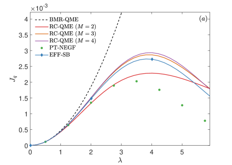
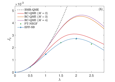
Figure 10: Steady state current as a function of coupling strength $\lambda$. We compare simulations of the RC-QME ($M=2-4$) to the BMR-QME (dashed), the PT-NEGF ($\circ$) and the EFF-SB ($\diamond$) methods. Parameters are $\epsilon=0$, $\Delta=1$, $\Lambda=1000\pi\Delta$. The temperatures are $T_{h}=\Delta$, $T_{c}=0.5\Delta$. (a) $\gamma=0.005$, $\Omega=10\Delta$. (b) $\gamma=0.005$, $\Omega=5\Delta$.

References

- (1) Di Ventra M 2008 Electrical Transport in Nanoscale Systems (Cambridge: Cambridge University Press)
- (2) Breuer H P and Petruccione F 2002 The theory of open quantum systems (New York: Oxford University Press)
- (3) Nitzan A 2006 Chemical Dynamics in Condensed Phases: Relaxation, Transfer, and Reactions in Condensed Molecular Systems (New York: Oxford University Press)
- (4) Hartmann R and Strunz W T 2020 Phys. Rev. A 101 012103
- (5) Nalbach P and Thorwart M 2010 The Journal of Chemical Physics 132 194111
- (6) Lee M K, Huo P and Coker D F 2016 Annual Review of Physical Chemistry 67 639
- (7) Xiang Z L, Ashhab S, You J and Nori F 2013 Reviews of Modern Physics 85 623–653
- (8) Strasberg P, Schaller G, Lambert N and Brandes T 2016 New Journal of Physics 18 073007
- (9) Friedman H M, Agarwalla B K and Segal D 2018 New Journal of Physics 20 083026
- (10) Newman D, Mintert F and Nazir A 2017 Phys. Rev. E 95 032139
- (11) Brenes M, Mendoza-Arenas J J, Purkayastha A, Mitchison M T, Clark S R and Goold J 2020 Physical Review X 10
- (12) Bergmann N and Galperin M 2020 arXiv e-prints (Preprint eprint 2004.05175)
- (13) Wiedmann M, Stockburger J T and Ankerhold J 2020 New Journal of Physics 22 033007
- (14) Motz T, Wiedmann M, Stockburger J T and Ankerhold J 2018 New Journal of Physics 20 113020
- (15) Segal D and Nitzan A 2005 Phys. Rev. Lett. 94 034301
- (16) Segal D 2006 Phys. Rev. B 73 205415
- (17) Senior J, Gubaydullin A, Karimi B, Peltonen J T, Ankerhold J and Pekola J P 2020 Communications physics 3
- (18) Velizhanin K A, Wang H and Thoss M 2008 Chemical Physics Letters 460 325–330
- (19) Nicolin L and Segal D 2011 The Journal of Chemical Physics 135 164106
- (20) Boudjada N and Segal D 2014 The Journal of Physical Chemistry A 118 11323
- (21) Segal D 2014 Phys. Rev. E 90 012148
- (22) Segal D and Agarwalla B K 2016 Annual Review of Physical Chemistry 67 185
- (23) Aurell E, Donvil B and Mallick K 2020 Phys. Rev. E 101 052116
- (24) Aurell E and Montana F 2019 Phys. Rev. E 99 042130
- (25) Wang C, Ren J and Cao J 2015 Scientific Reports 5
- (26) Wang C, Ren J and Cao J 2017 Phys. Rev. A 95 023610
- (27) Velizhanin K A, Thoss M and Wang H 2010 The Journal of Chemical Physics 133 084503
- (28) Yang Y and Wu C Q 2014 Euro. Phys. Lett 107 30003
- (29) Agarwalla B K and Segal D 2017 New Journal of Physics 19 043030
- (30) Liu J, Xu H, Li B and Wu C 2017 Phys. Rev. E 96 012135
- (31) Yang C H and Wang H 2020 Entropy 22
- (32) Segal D 2013 Phys. Rev. B 87 195436
- (33) Kilgour M, Agarwalla B K and Segal D 2019 The Journal of Chemical Physics 150 084111
- (34) Saito K and Kato T 2013 Phys. Rev. Lett. 111 214301
- (35) Yamamoto T, Kato M, Kato T and Saito K 2018 New Journal of Physics 20 093014
- (36) Cerrillo J, Buser M and Brandes T 2016 Phys. Rev. B 94 214308
- (37) Song L and Shi Q 2017 Phys. Rev. B 95 064308
- (38) Kato A and Tanimura Y 2016 The Journal of Chemical Physics 145 224105
- (39) Xu M, Stockburger J T and Ankerhold J 2020 arXiv e-prints (Preprint eprint arXiv:2012.11942)
- (40) Kelly A 2019 The Journal of Chemical Physics 150 204107
- (41) Liu J, Hsieh C Y, Segal D and Hanna G 2018 The Journal of Chemical Physics 149 224104
- (42) Carpio-Martínez P and Hanna G 2019 The Journal of Chemical Physics 151 074112
- (43) Carpio-Martínez P and Hanna G 2021 The Journal of Chemical Physics 154 094108
- (44) Prior J, Chin A W, Huelga S F and Plenio M B 2010 Phys. Rev. Lett. 105 050404
- (45) Woods M P, Groux R, Chin A W, Huelga S F and Plenio M B 2014 Journal of Mathematical Physics 55 032101
- (46) Tamascelli D, Smirne A, Lim J, Huelga S F and Plenio M B 2019 Phys. Rev. Lett. 123 090402
- (47) Chen T, Balachandran V, Guo C and Poletti D 2020 Phys. Rev. E 102 012155
- (48) Tamascelli D, Smirne A, Huelga S F and Plenio M B 2018 Phys. Rev. Lett. 120 030402
- (49) Pleasance G, Garraway B M and Petruccione F 2020 Phys. Rev. Research 2 043058
- (50) Fruchtman A, Lovett B W, Benjamin S C and Gauger E M 2015 New Journal of Physics 17 023063
- (51) Schönleber D W, Croy A and Eisfeld A 2015 Phys. Rev. A 91 052108
- (52) Lambert N, Ahmed S, Cirio M and Nori F 2019 Nature Communications 10 4656
- (53) Iles-Smith J, Lambert N and Nazir A 2014 Phys. Rev. A 90 032114
- (54) Iles-Smith J, Dijkstra A G, Lambert N and Nazir A 2016 The Journal of Chemical Physics 144 044110
- (55) Strasberg P, Schaller G, Schmidt T L and Esposito M 2018 Phys. Rev. B 97(20) 205405
- (56) Restrepo S, Böhling S, Cerrillo J and Schaller G 2019 Phys. Rev. B 100 035109
- (57) Nazir A and Schaller G 2018 The Reaction Coordinate Mapping in Quantum Thermodynamics (Springer International Publishing) pp 551–577
- (58) Chen F, Arrigoni E and Galperin M 2019 New Journal of Physics 21 123035
- (59) Correa L A, Xu B, Morris B and Adesso G 2019 The Journal of Chemical Physics 151 094107
- (60) Yan Y and Xu R 2005 Annual Review of Physical Chemistry 56 187–219
- (61) This comment is meant to explain seemingly odd values selected for parameters, and . Most importantly, these parameters satisfy , beneficial for the effective spin–boson description, and , allowing us to use the RC–QME weak coupling method. Specific values for and were originally chosen based on parameters in the rotated picture, described in Appendix B. However, since we do not show results in the rotated basis, this reference point is irrelevant and inconsequential.
- (62) Weiss U 1999 Quantum Dissipative Systems (Singapore:World Scientific)