Dissipative Bethe Ansatz: Exact Solutions of Quantum Many-Body Dynamics Under Loss

Abstract

We use the Bethe Ansatz technique to study dissipative systems experiencing loss. The method allows us to exactly calculate the Liouvillian spectrum. This opens the possibility of analytically calculating the dynamics of a wide range of experimentally relevant models including cold atoms subjected to one and two body losses, coupled cavity arrays with bosons escaping the cavity, and cavity quantum electrodynamics. As an example of our approach we study the relaxation properties in a boundary driven XXZ spin chain. We exactly calculate the Liouvillian gap and find different relaxation rates with a novel type of dynamical dissipative phase transition. This physically translates into the formation of a stable domain wall in the easy-axis regime despite the presence of loss. Such analytic results have previously been inaccessible for systems of this type.

Introduction– Particle loss is an important mechanism of environmental dissipation. It strongly affects the dynamics of many particle systems in the classical and the quantum regimes and has immense impact on technological applications. It is present in numerous experimental platforms including cold atoms Gross and Bloch (2017); Lewenstein et al. (2007), non-linear waveguides Zezyulin et al. (2012), coupled cavity arrays Fitzpatrick et al. (2017); Tangpanitanon et al. (2016, 2019); Wolff et al. (2016), THz cavities Zhang et al. (2016); Scalari et al. (2012); Halati et al. (2019); Schlawin et al. (2019), quantum wires Fröml et al. (2019); Lebrat et al. (2019), condensed matter systems Mitrano et al. (2014), and solid-state devices De Franceschi et al. (2010). Indeed, the primary source of dissipation in these settings is a consequence of particles escaping from the system either through one- or two-body processes Lewenstein et al. (2007), or due to the coupling to an external electromagnetic field (e.g. Zhang et al. (2016); De Franceschi et al. (2010); Fitzpatrick et al. (2017)). The platforms underlie future quantum technologies, which will require efficient manipulation of many constituents.

Understanding the behaviour of such systems is of paramount importance, and sheds light on properties that are robust to dissipation and could therefore allow for more efficient methods of information storage and the development of novel error correction mechanisms. However, due to the exponential complexity, numerical simulations of these systems are challenging. Thus, gaining a better understanding of their properties through uncovering their analytical structure is highly desirable. Thus far, exact solutions of such systems have been limited only to the stationary states of boundary driven systems Prosen (2011a, b); Popkov and Prosen (2015); Ilievski (2014, 2017); Ilievski and Prosen (2014); Ilievski and Žunkovič (2014); Žunkovič (2014); Lenarčič and Prosen (2015); Karevski et al. (2013); Popkov and Schütz (2017); Yuge and Sugita (2015); Popkov et al. (2019); Vanicat et al. (2018); Buča and Prosen (2014); Nigro (2020); Prosen (2015); Diehl et al. (2008); Buča and Prosen (2018) and to those with non-interacting Hamiltonians Žnidarič (2011, 2014, 2010); Prosen (2008); Prosen and Seligman (2010); Manzano et al. (2016); Monthus (2017); Krapivsky et al. (2019); Carollo et al. (2017); Budich et al. (2015); Iemini et al. (2016); Medvedyeva and Kehrein (2014); Guo and Poletti (2017); Medvedyeva et al. (2016); Rowlands and Lamacraft (2018); Ziolkowska and Essler (2020); Shibata and Katsura (2019a, b). Beyond this only certain approximate methods van Caspel and Gritsev (2018); Bastianello et al. (2020); Lange et al. (2017); Lenarčič et al. (2018), e.g. introducing dissipation on hydrodynamical scales, are available.

In this Letter we go beyond these results and develop an analytic approach to describing the dynamics of a wide class of fully interacting dissipative systems. Our approach opens a novel avenue for the analytical study of experimentally relevant many-body models experiencing loss, provided that the system’s effective non-Hermitian Hamiltonian is integrable. In experimental settings, examples of systems treatable by our method can be found in cold atom quantum simulators subjected to single and two body losses Gross and Bloch (2017); Lewenstein et al. (2007); Zhang et al. (2016), and driven-dissipative cavity arrays of bosons Fitzpatrick et al. (2017).

As an example of the power of our method we study the instructive and paradigmatic XXZ spin chain, often used to describe limiting cases of the aforementioned experimental setups Lewenstein et al. (2007), which we subject to boundary spin loss. We find that our model exhibits intriguing physical phenomena. Additionally, these types of localized loss processes recently attracted a lot of theoretical and experimental interest due to their importance for understanding transport properties and as an experimentally realistic venue for preparing interesting quantum states, see e.g. Tonielli et al. (2019); Kuhr (2016); Damanet et al. (2019); Zezyulin et al. (2012); Barontini et al. (2013); Lebrat et al. (2019); Fröml et al. (2019); Wolff et al. (2020); Prosen (2011a); Buča and Prosen (2014, 2012, 2017, 2018); Mendoza-Arenas et al. (2014).

Using our method we first characterize the relaxation dynamics, uncovering a dynamical dissipative phase transition Horstmann et al. (2013), by calculating the closure of the Liouvillian gap. Next, we analytically show the presence of a novel type of dynamical dissipative phase transition that corresponds to non-analiticity in many relaxation rates beyond the leading decay mode. Physically this implies a transition in the dynamics on both short and asymptotic time scales. This should be contrasted with phase transitions in the statationary state Kessler et al. (2012); Bhaseen et al. (2012); Marcuzzi et al. (2014); Casteels et al. (2017) or the leading decay mode Horstmann et al. (2013). In our case the stationary state is always the same and a phase transition occurs in the leading decay mode and in other parts of the spectrum. Related to this, we show that a stable domain wall state is formed in the easy-axis regime. Interestingly, the domain wall formation occurs spontaneously if the system is initialized in the maximally polarized state. It arises as a consequence of boundary bound states that we solve for. Formation of domain walls in both integrable and non-integrable closed systems has also recently attracted considerable interest Collura et al. (2018); Gamayun et al. (2019); Misguich et al. (2019); Medenjak and De Nardis (2020); Collura et al. (2020), but is currently still analytically unsolved.

Solving lossy models– We will focus on systems described by the Lindblad master equation which characterizes open quantum systems in the weak system-bath coupling limit. The dynamics of the density matrix $\rho$ is provided by the generator $\mathcal{L}$ as Breuer et al. (2002); Gardiner et al. (2004),

$$\frac{{\rm d}}{{\rm d}t}\rho(t)={{\cal L}}\rho(t):=$$

$$-{\rm i}[H,\rho(t)]+\sum_{\mu}\left(2L_{\mu}\rho(t)L_{\mu}^{\dagger}-\{L_{\mu}^{\dagger}L_{\mu},\rho(t)\}\right),$$ (1)

where $H$ is the system Hamiltonian and $L_{\mu}$ are the Lindblad jump operators modeling the influence of the environment on the system. The time evolution of an observable $O$ can be computed by diagonalizing the generator ${{\cal L}}$, ${\langle O(t)\rangle}={{\rm tr}}(O\rho(t))=\sum_{\mu}e^{\lambda_{\mu}t}{{\rm tr}}(\tilde{\rho}^{\dagger}_{\mu}\rho(0)){{\rm tr}}(\rho_{\mu}O)$, where $\lambda_{\mu}$ are the eigenvalues and $\rho_{\mu},\tilde{\rho}_{\mu}$ the right and left eigenvectors.

The general setup that we consider comprises an integrable Hamiltonian $H$ with a conservation law $M$ and Lindblad operators $L_{\mu}$ that change the eigenvalue of $M$ by well-defined amounts $m_{\mu}>0$, $[M,L_{\mu}]=-m_{\mu}L_{\mu}$, inducing the loss of the quantity $M$ in the system. For instance $M$ can be the total particle number and $L_{\mu}$ particle annihilation operators. In the following we will discuss the integrability requirements for applying our technique. The Liouvillian superoperator can be represented on the vector space with doubled degrees of freedom by the channel-state transformation $\mathinner{|{\psi}\rangle}\mathinner{\langle{\phi}|}\to\mathinner{|{\psi}\rangle}\otimes\mathinner{|{\phi}\rangle}$, yielding

$${{\cal L}}=-i(H\otimes\mathbbm{1}-\mathbbm{1}\otimes H^{T})++\sum_{\mu}\left(2L_{\mu}\otimes L_{\mu}^{*}-L_{\mu}^{\dagger}L_{\mu}\otimes\mathbbm{1}-\mathbbm{1}\otimes(L_{\mu}^{\dagger}L_{\mu})^{T}\right).$$ (2)

We will show that in order to obtain eigenvalues of the Liouvillian it suffices to obtain eigenvalues $E_{j}$ of the non-hermitian Hamiltonian $\tilde{H}\equiv-{\rm i}H-\sum_{\mu}L_{\mu}^{\dagger}L_{\mu}$ Torres (2014); Briegel and Englert (1993). Since $[\tilde{H},M]=0$, we can assume that the eigenvectors $\mathinner{|{\psi_{j}}\rangle}$ of $\tilde{H}$ are also eigenvectors of $M$. The generator (2) can now be decomposed into two parts

$${{\cal L}}=\mathcal{H}+\mathcal{D},$$ (3)

with $\mathcal{H}\equiv\tilde{H}\otimes\mathbbm{1}+\mathbbm{1}\otimes\tilde{H}^{*}$ and $\mathcal{D}=2\sum L_{\mu}\otimes L_{\mu}^{*}$. Since $\mathcal{H}$ is a sum of two operators acting on the factors in a tensor product independently, its eigenvalues read $\mathcal{H}\mathinner{|{\psi_{i}}\rangle}\otimes\overline{\mathinner{|{\psi_{j}}\rangle}}=(E_{i}+E_{j}^{*})\mathinner{|{\psi_{i}}\rangle}\otimes\overline{\mathinner{|{\psi_{j}}\rangle}}.$ Let us now order the eigenvectors $\mathinner{|{\psi_{i}}\rangle}\otimes\overline{\mathinner{|{\psi_{j}}\rangle}}$ of $\mathcal{H}$ by the corresponding eigenvalues $m_{i,j}$ of $\mathcal{M}\equiv M\otimes\mathbbm{1}+\mathbbm{1}\otimes M$. Due to the purely lossy dynamics the nondiagonal matrix elements of $\mathcal{D}$ lie strictly above the diagonal. This immediately implies that ${{\cal L}}$ takes the upper triangular form in the basis $\mathinner{|{\psi_{i}}\rangle}\otimes\overline{\mathinner{|{\psi_{j}}\rangle}}$ and that the eigenvalues of the Liouvillian $\lambda_{i,j}=E_{i}+E_{j}^{*}$ coincide with those of $\mathcal{H}$. Thus, provided that the non-hermitian Hamiltonian $\tilde{H}=-{\rm i}H-\sum_{\mu}L_{\mu}^{\dagger}L_{\mu}$ is exactly solvable, we have found the full spectrum of the Liouvillian. Nevertheless, the structure of Liouvillian eigenvectors corresponding to the eigenvalue $\lambda_{i,j}$ is more complicated and includes the states $\mathinner{|{\psi_{k}}\rangle}\otimes\overline{\mathinner{|{\psi_{l}}\rangle}}$, with $m_{k,l}\leq m_{i,j}$ SM .

Note that the dynamics describing pure gain can be treated on the same footing.

Here we focus on using Bethe Ansatz techniques Bethe (1931); Korepin et al. (1997) for solving $\tilde{H}$, which are applicable to a wide range of models. In many physically relevant situations the dissipative contribution, $\sum_{\mu}L_{\mu}^{\dagger}L_{\mu}$, modifying the system’s integrable Hamiltonian, $H$, will leave $\tilde{H}$ integrable. For instance, single particle bulk loss throughout the system in any integrable model with particle number conservation, the dissipative contribution corresponds simply to the particle number operator, which clearly implies integrability of $\tilde{H}$. For two-level systems with conserved magnetization the $L_{\mu}$ would correspond to on-site spin lowering operators. This is known to be a primary dissipative loss mechanism in numerous experimental setups such as optical lattices (due to interactions with the background vacuum), wave guides, solid state contacts, and coupled cavity arrays Lewenstein et al. (2007); Zezyulin et al. (2012); Fitzpatrick et al. (2017); De Franceschi et al. (2010). Other examples of dissipative mechanisms that preserve integrability of $\tilde{H}$ are provided by nearest-neighbour dissipation Parmee and Cooper (2018, 2019) and two-body loss processes Lewenstein et al. (2007); Nakagawa et al. (2020) (for details see SM ).

It is instructive to contrast this situation with cases where the full Liouvillian can be mapped to a non-Hermitian integrable Hamiltonian Medvedyeva et al. (2016); Ziolkowska and Essler (2020); Rowlands and Lamacraft (2018); Shibata and Katsura (2019a, b) (where the physical system’s Hamiltonian is quadratic). In our case the system’s Hamiltonian is interacting and the full Liouvillian does not correspond to some non-Hermitian integrable Hamiltonian. Rather here it is only $\tilde{H}$ (and hence $\mathcal{H}$ in Eq. (3)) that is integrable. For conciseness and in order to demonstrate the utility of our method we will now focus on the example of the Heisenberg XXZ chain in the presence of a spin sink at a single boundary.

Boundary driven XXZ spin chain dynamics– The Heisenberg Hamiltonian reads

$$H_{XXZ}=\sum_{j=1}^{N-1}\sigma^{x}_{j}\sigma^{x}_{j+1}+\sigma^{y}_{j}\sigma^{y}_{j+1}+\Delta\sigma^{z}_{j}\sigma^{z}_{j+1},$$ (4)

where the Pauli spin$-{\textstyle\frac{1}{2}}$ operators are $\sigma^{x,y,z}$, $\Delta$ is the anisotropy, and $N$ is the number of spin sites. We study the setup with an arbitrary loss rate on the first site $L_{1}=2\sqrt{\Gamma}\sigma^{-}_{1}$. The corresponding non-Hermitian Hamiltonian reads

$$\tilde{H}=-{\rm i}H_{XXZ}-4\Gamma\sigma^{z}_{1}+\rm{const},$$ (5)

i.e. ${\rm i}\tilde{H}$ describes an XXZ spin chain Hamiltonian in the presence of an imaginary magnetic field at the boundary. The Hamiltonian has a $U(1)$ symmetry $M=\sum_{j}\sigma^{z}_{j}$ and $[M,L_{1}]=-L_{1}$, i.e. $m_{1}=1$.

In contrast to boundary driven spin chains Prosen (2011a, b); Popkov and Prosen (2015); Žnidarič (2011); Prosen and Žunkovič (2010); Mendoza-Arenas et al. (2019); Žnidarič et al. (2017); Mendoza-Arenas et al. (2015, 2013) the stationary state, ${{\cal L}}\rho_{\infty}=0$, is not of interest in our system since it is a trivial vacuum state. However, we obtain the full spectrum of the non-Hermitian Hamiltonian Eq. (5), and therefore of the Liouvillian by the Bethe ansatz. The Bethe equations were obtained using Sklyanin’s reflection algebra Sklyanin (1988), and equivalently the coordinate Bethe ansatz Korepin et al. (1997); Ragoucy (2012); Crampé et al. (2010) (with imaginary boundary magnetic field $4i\Gamma\sigma^{z}_{1}$).

The complex energies of $\tilde{H}$ corresponding to $m$ magnons read

$$E(\{k_{j}\})=-{\rm i}(N-1)-4{\rm i}\sum_{j=1}^{m}(\cos(k_{j})-\Delta),$$ (6)

where the momenta of the magnons, $\{k_{j}\}$, are obtained by solving the Bethe equations

$$\frac{e^{2iNk_{j}}(\Delta-e^{ik_{j}})(e^{ik_{j}}+2i\Gamma-\Delta)}{(e^{ik_{j}}\Delta-1)(1+e^{ik_{j}}(2i\Gamma-\Delta))}=\prod_{l\neq j}^{m}S(e^{ik_{j}},e^{ik_{l}}).$$ (7)

The scattering matrix of two magnons takes the form

$$S(a,b)=\frac{(a-2\Delta ab+b)(1-2\Delta a+ab)}{(a-2\Delta+b)(1-2\Delta b+ab)}.$$ (8)

From the triangular form of the Liouvillian, which couples different magnetization sectors, we can express its eigenstates in terms of Bethe states of $\tilde{H}$ by simplified Gaussian elimination (for details see SM ). For later convenience we introduce a pair of labels $(m_{L},m_{R})$ refering to the eigenstates of ${{\cal L}}$ comprised of tensor product of two Bethe states with $m_{L}$ and $m_{R}$ magnons as well as tensor products of Bethe states with less $q_{L}<m_{L}$ and $q_{R}<m_{R}$ magnons (see SI SM ). In what follows we will utilise our results to address two physically interesting questions.

Eigenvalue Structure and the Liouvillian gap— The first problem that we consider is the Liouvillian gap, $R$, of ${{\cal L}}$. It corresponds to the maximum real part of the eigenvalues different from 0, which is the inverse relaxation time of the longest-lived eigenmodes. We plot it in Fig. 1 for different values of the anisotropy parameter $\Delta$.

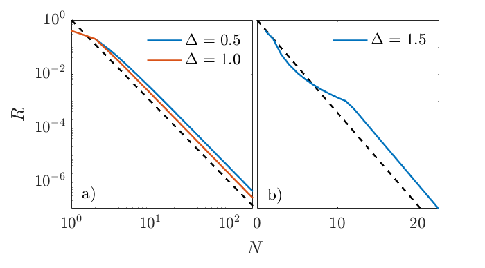
Figure 1: Scaling of the Liouvillian gap, $R$, with system size for $\Gamma=0.1$. a) Power law closing of the gap for $\Delta\leq 1$ with $R\propto 1/N^{3}$ (dashed line) shown for comparison. b) Exponential closing of the gap for $\Delta>1$ with $R\propto e^{-\alpha N}$ (dashed line) and $\alpha\approx 0.784$ shown for comparison.

The scaling of the gap with the system size $N$ is one of the primary features of open quantum systems, governing the late time dynamics.

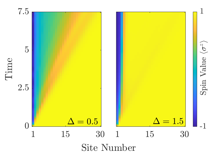
(a)

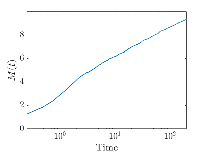
(b)

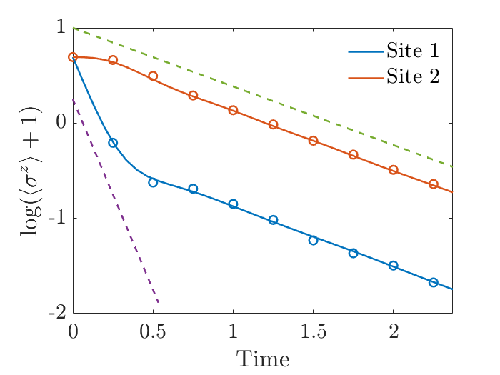
(c)

Figure 2: Domain wall formation and spin loss. a) Magnetization along the chain as a function of time for an initially fully polarized state with $\Gamma=0.5$. For $\Delta=0.5$ the initial state rapidly decays to the vacuum state $\rho_{\infty}$, while for $\Delta=1.5$ the system forms a meta-stable domain wall which decays exponentially slowly. b) The total spin lost, $M(t)$, by a 30 site system with $\Gamma=0.5$. This is logarithmic in time as a result of the domain wall preventing spin from leaking out. c) The spin decay on the first and second sites in 10 (solid) and 30 (circles) site systems with $\Delta=1.5$, $\Gamma=0.5$. We also plot the infinite chain 0 and 1 top-magnon decay rates in purple and green respectively for comparison.

We observe that the gap for $\Delta\leq 1$ corresponds to the eigenstates of ${{\cal L}}$ with $m_{L}+m_{R}=1$. By examining the single magnon $m=1$ solutions of (7) on top of the steady state we find that, depending on the value of $\Delta$, the gap closes at different rates. In particular, we demonstrate that for $\Delta\leq 1$ the longest lived excitations correspond to the solutions with $\lim_{N\to\infty}{\,{\rm Im}\,}(k_{j})=0$. Rewriting Eq. (7) as, $2ik=\frac{\Omega(e^{{\rm i}k})}{N}-\frac{2{\rm i}\pi I_{1}}{N},$ with $\Omega(a)=\log\left(\frac{(a\Delta-1)(-1+a(\Delta-2{\rm i}\Gamma))}{(a-\Delta)(a+2{\rm i}\Gamma-\Delta)}\right)$, we find that for $\Delta\leq 1$ the real part of the eigenvalues with the smallest real part scale as, SM ,

$$R=-\frac{1}{N^{3}}\frac{8\pi^{2}\Gamma}{4\Gamma^{2}+(\Delta+1)^{2}}+{\cal O}(\frac{1}{N^{4}}).$$ (9)

This matches the scaling of the gap for free fermions Prosen (2008). In the $N\to\infty$ limit these solutions are straightforwardly generalized to $m$-magnons SM . However, for $\Delta>1$ the leading decay rate is not in this class of solutions. Instead, we find exponentially long relaxation times consistent with a gap that closes exponentially fast (see Fig. 1 and SM ).

Boundary bound states and domain wall formation in the easy-axis regime— In the second setup we consider the case where the system is initialized in a highly excited, i.e. maximally polarized (all spins-up) state. In this case, due to the structure of ${{\cal L}}$, we need only consider eigenstates with $m_{L}=m_{R}=m$ (see SM ). In order to study the dynamics we now focus on the most stable (maximum real part) eigenvalues in the $m$ top-magnon sector, corresponding to spin-down excitations on top of the all spins-up state. The Bethe equations for top-magnons can be obtained from Eq. (7) by replacing $\Gamma\to-\Gamma$ in the sector with $m$ magnons.

Focusing on the easy-axis, $\Delta>1$, regime, we show that in the $m$ top-magnon sector states with $\lim_{N\to\infty}{\,{\rm Im}\,}(k_{j})>0$, which are localized at the boundary appear and are the most stable (see SI SM ). For these bound states the $m$ top-magnon Bethe equations can be easily solved in the $N\to\infty$ limit, since $e^{{\rm i}k_{j}N}\to 0$ (see SI SM ). A recursive solution of

$$\exp(-{\rm i}k_{j})+\exp(ik_{j-1})=2\Delta,$$

$$\exp(-{\rm i}k_{1})=\Delta+2{\rm i}\Gamma,$$

gives an appealingly simple result for the leading Liouvillian eigenvalues in the $m$ top-magnon sector,

$$\lambda_{m}=-2{\rm i}(\exp({\rm i}k_{m})-\exp(-{\rm i}k^{*}_{m})).$$ (10)

Physically this means that the first top-magnon with momentum $k_{1}$ is localized near the loss site, while the $j$th top-magnon is recursively bound to the $(j-1)$st. Importantly, we can show that as the number of top-magnons is increased they become exponentially stabilized, i.e. $\lim_{m\to\infty}{\,{\rm Re}\,}{\lambda_{m}}=0$ (see SI SM ). In turn, this implies that exponentially large times (in $m$) are needed for the loss site to dissipate the state with $m$ top-magnons.

The existence of these boundary bound states has intriguing physical consequences. It results in domain wall formation if the system is initialized in the maximally polarized state. Naively one might think that such a state is the most unstable, however tDMRG simulations, as shown in Fig. 2(a), in the $\Delta>1$ regime reveal that the total spin leaking out of the system increases only logarithmically with time (see Fig. 2(b)). This can be understood as a consequence of exponential stability of the boundary bound states. Namely, that exponentially long times (in $m$) are required for the loss site to remove all the states with $m$ down-turned spins. Moreover, in Fig. 2(c) we show that the dynamics of magnetization close to the spin loss site is well described by the decay rates of boundary top-magnons. On the other hand the decay of the maximally polarized state in the $\Delta<1$ regime is very rapid (Fig. 2(a)), and the total loss of magnetization increases linearly with time. There have recently been a number of studies addressing the dynamics of domain walls in integrable Collura et al. (2018); Gamayun et al. (2019); Misguich et al. (2019); Collura et al. (2020) and nonintegrable Medenjak and De Nardis (2020) systems without dissipation. While the ballistic expansion in the $\Delta<1$ regime is well understood, the domain wall freezing was analytically unresolved.

The existence of boundary bound states also has profound consequences on the spectral properties of ${{\cal L}}$. It results in a dissipative phase transition (shown in Fig. 3). In contrast to standard dissipative phase transitions Kessler et al. (2012), the stationary state remains the same (all spins-down). The phase transition rather happens in the relaxation spectrum of ${{\cal L}}$ at different values of $\Delta$ and $\Gamma$ depending on the top-magnon number $m$, and converges to $\Delta=1$ in the limit $m\to\infty$. This is similar to dynamical dissipative phase transitions Horstmann et al. (2013), but the discontinuous eigenvalues that are relevant for the dynamics are not only the Liouvillian gap. This is reflected in the fact that already the short time dynamics for the easy-plane and easy-axis regimes are qualitatively different (see Fig. 2) The discontinuity is shown in Fig. 3 where we can see non-analyticity in eigenvalues in three different top-magnon sectors demonstrating that this phase transitions happens in all sectors. The non-analyticity shown corresponds to the non-existence of boundary bound state solutions for $\Delta<1$. More specifically, we prove the existence of $\{k_{j}\}$ such that $\lim_{\Delta\to 1}\frac{dk_{j}}{d\Delta}\to\infty$ for large $N$ and small $\Gamma$ (see SI SM ), which implies the divergence in the corresponding eigenvalues.

Conclusion— We have devoloped a framework for diagonalizing quantum Liouvillians with integrable system Hamiltonians and dissipative loss. We demonstrate the utility of our method in an example of the Heisenberg XXZ spin chain with boundary loss. The method allows us to directly identify phase transitions in the Liouvillian spectrum and calculate the Liouvillian gap. This led us to observe two intriguing physical phenomena, namely domain wall formation, and a dissipative phase transition, which we link to the existence of boundary bound top-magnons. Such remarkable phenomena could occur in other models with localized loss, e.g. 1D Hubbard and interacting bosons in 1D Lewenstein et al. (2007), which can be studied analytically with our method.

A number of questions remain open. The first natural extension of our results is directly calculating the full eigenstates of the quantum Liouvillian. We also envisage using the thermodynamic Bethe ansatz van Tongeren (2016); Yang and Yang (1969) to explore the decay of states with a finite density of excitations, and the connection with boundary states Grijalva et al. (2019) and strong edge modes Fendley (2016) in closed systems. Additionally, the Liouvillian spectrum exhibits a multi-band structure at sufficiently large $\Delta$ (see Fig. S1 in SM ), which remains to be explained.

More generally our method can be applied to a number of systems that are quantitatively very different from the example we studied. Such systems include, for example, arrays of two-level systems with nearest-neighbor dissipation induced by external drive Parmee and Cooper (2018), and integrable systems exhibiting the loss of particles at each site Lewenstein et al. (2007). Here the interest is two-fold. On one hand, judging by our example, such systems hide a plethora of interesting physical phenomena, which are yet to be uncovered. On the other hand they describe realistic experimental setups and therefore provide an indispensable tool for understanding future experiments.

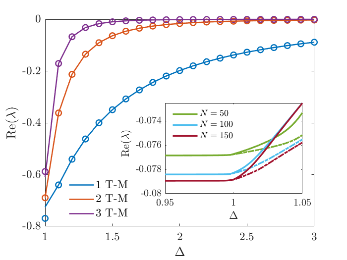
Figure 3: The eigenvalues with maximum real part of ${{\cal L}}$ when $N\rightarrow\infty$ (circles) from Equation (10) for $\Delta>1$ compared with a 50 site system (line) for 1, 2 and 3 top-magnon sectors at $\Gamma=0.01$. The inset shows the largest (solid line) and second largest (dashed line) real part of the eigenvalues of the Liouvillian in the one top-magnon sector for different $N$ at $\Gamma=0.01$. We see a cusp forming with increasing $N$ close to $\Delta=1$ indicating the dynamical dissipative phase transition in the large $N$ limit.

Note Added: While nearing the completion of this manuscript a related preprint appeared Nakagawa et al. (2020) studying exact solutions in the Hubbard model with two-body loss.

Acknowledgments— We thank F. Essler, E. Ilievski, C. Parmee, T. Prosen, J. Tindall, F. Tonielli, and A. Ziolkowska for useful discussions. We are in particularly indebted to T. Prosen for suggesting the original problem that led to this study. BB, CB and DJ acknowledge funding from EPSRC programme grant EP/P009565/1, EPSRC National Quantum Technology Hub in Networked Quantum Information Technology (EP/M013243/1), and the European Research Council under the European Union’s Seventh Framework Programme (FP7/2007-2013)/ERC Grant Agreement no. 319286, Q-MAC.

Supplementary Information: Exact Solutions of Quantum Many-Body Dynamics Under Loss using the Bethe Ansatz

In the supplemental material we provide the discussion of technical details that were omitted from the main text. In the first part we discuss further examples of systems solvable by our method. In the second section we construct the eigenstates of the Liouvillian. In the third section we provide details on the calculation of the Liouvillian gap, and in the final section the results related to the boundary magnons. We also plot the full Liouvillian spectrum for different values of anisotropy $\Delta$ which shows the formation of intriguing band structure (see Fig. S1).

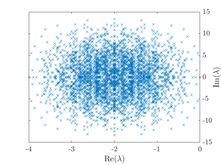
(a) $\Delta=0.5$

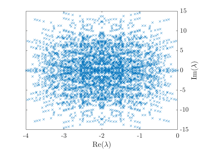
(b) $\Delta=1.0$

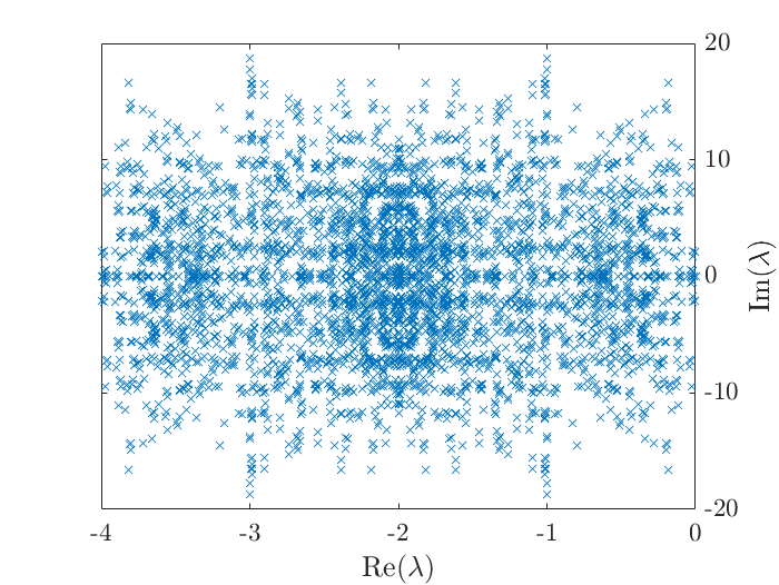
(c) $\Delta=1.5$

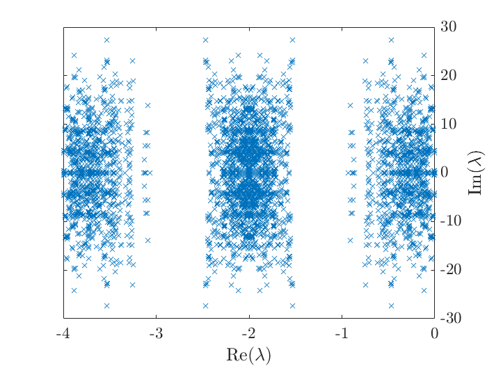
(d) $\Delta=2.5$

Figure S1: Full spectrum for a 6 site system with $\Gamma=0.5$ at various $\Delta$. We see the emergence of band structure forming as $\Delta$ increased. This corresponds to different subspaces of the Hilbert space decaying in separate stages.

Examples of dissipative quantum models solvable by Bethe ansatz

Here we provide some further examples of models solvable by the method introduced in the main text.

Consider a general 1D Hamiltonian with raising (lowering) operators for possibly several species, $a_{j}^{\dagger}$, $b_{j}^{\dagger},\ldots$ ($a_{j},b_{j},\ldots$), acting on site $j=1,\ldots,N$. We further assume that $[H,\sum a^{\dagger}_{j}a_{j}]=[H,\sum b^{\dagger}_{j}b_{j}]=0$. We define the dissipative contribution to $\tilde{H}$ as $D\equiv\sum_{\mu}L_{\mu}^{\dagger}L_{\mu}$. Taking an integrable $H$ we observe that the following types of loss processes render $\tilde{H}$ integrable,

1. $L_{j}=\gamma a_{j}b_{j},j=1,\ldots,N$ (homogenous two-body loss),

2. $L_{j}=\gamma a^{\dagger}_{j}a_{j+1},L_{j+N-1}=\gamma^{\prime}a_{j}a^{\dagger}_{j+1},j=1,\ldots,N-1$ (dissipative nearest-neighbor hopping) and,

3. $D=\gamma\sum_{j=1}^{N-1}a^{\dagger}_{j}a_{j+1}$ (correlated non-local dissipative loss).

The $\tilde{H}$ in cases 1. (2.) are integrable because $D$ may be rewritten as an imaginary interaction term of the form $D=\sum_{j}a^{\dagger}_{j}a_{j}b^{\dagger}_{j}b_{j}$ ($D=\sum_{j}\gamma a_{j}a^{\dagger}_{j}a^{\dagger}_{j+1}a_{j+1}+\gamma^{\prime}a^{\dagger}_{j}a_{j}a_{j+1}a^{\dagger}_{j+1}$). In particular, homogeneous two-body loss is a standard loss process in cold atom simulations Lewenstein et al. (2007); Gross and Bloch (2017). A concrete physical example of this is the 1D Hubbard model with two-body recombination of fermions of spin-down and spin-up Nakagawa et al. (2020).

The case  3. has an integrable $\tilde{H}$ because $D$ is just an imaginary contribution to the hopping (kinetic) term in $H$. For instance, for XXZ spin chains such a non-Hermitian Hamiltonian was solved in Beisert et al. (2013). These cases are realized, for instance, by two-level systems coupled by dipolar interactions and subject to nonlocal dissipation, i.e. decay through optical emissions Parmee and Cooper (2018, 2019).

Eigenstates of the boundary loss XXZ Liouvillian

In this section we will construct the right eigenstates of the Liouvillian

$${{\cal L}}=-i(H\otimes\mathbbm{1}-\mathbbm{1}\otimes H^{T})+\sum_{k}\left(2L_{\mu}\otimes L_{\mu}^{*}-L_{\mu}^{\dagger}L_{\mu}\otimes\mathbbm{1}-\mathbbm{1}\otimes(L_{\mu}^{\dagger}L_{\mu})^{T}\right).$$ (S1)

In the case of the XXZ chain with a single loss at the first site. First of all, we will remind the reader of the basic structure of Bethe eigenstates, which will then serve to construct the eigenstates of the Liouvillian. The eigenstate of the Hamiltonian

$$\tilde{H}=-{\rm i}H_{XXZ}-\Gamma\sigma^{+}_{1}\sigma^{-}_{1},$$ (S2)

pertaining to the energy $E_{\phi_{\eta}^{a}}$ reads

$$\mathinner{|{\phi^{a}_{\eta}}\rangle}=\sum_{1\leq x_{1}<...<x_{a}\leq n}f_{a,\eta}(x_{1},..,x_{a})\mathinner{|{x_{1},...,x_{a}}\rangle}.$$ (S3)

Here the set of $\{x_{j}\}$ indicate the positions of spin-up excitations while the label $a$ corresponds to a given total magnetisation. Finally $\eta$ labels the state within this sector. In terms of Bethe roots $\{k_{j}\}$, the wave function reads

$$f(x_{1},...,x_{m})=\sum_{P}\varepsilon_{P}A(k_{1},...,k_{m})e^{i(k_{1}x_{1}+\dots k_{m}x_{m})}$$ (S4)

$$A(k_{1},...,k_{m})=\prod_{j=1}^{m}(\Delta e^{-ik_{j}N}-e^{-i(N+1)k_{j}})\prod_{1\leq j<l\leq m}B(-k_{j},k_{l})e^{-ik_{l}}$$ (S5)

$$B(k,k^{\prime})=(1-2\Delta e^{ik^{\prime}}+e^{i(k+k^{\prime})})(1-2\Delta e^{-ik}+e^{i(k^{\prime}-k)}),$$ (S6)

where the summation is performed over all permutations and negations of $\{k_{j}\}$, and $\varepsilon_{P}$ changes sign with each such mutation.

We then use the triangular form for the Liouvillian, i.e that

$${\mathcal{L}}:\mathcal{M}^{a}\otimes\mathcal{M}^{b}\rightarrow\left(\mathcal{M}^{a}\otimes\mathcal{M}^{b}\right)\oplus\left(\mathcal{M}^{a-1}\otimes\mathcal{M}^{b-1}\right),$$ (S7)

where $\mathcal{M}^{a}$ is the subspace with magnetization $a$, to make the ansatz that the eigenstate of ${\mathcal{L}}$ with eigenvalue $E_{\phi_{\eta}^{a}}+E_{\phi_{\zeta}^{b}}^{*}$ is given by

$$\mathinner{|{\Phi_{\eta,\zeta}^{a,b}}\rangle}=\mathinner{|{\phi_{\eta}^{a}}\rangle}\overline{\mathinner{|{\phi_{\zeta}^{b}}\rangle}}+\sum_{\mu=1}^{\min\{a,b\}}\sum_{i,j}B_{\mu}(i,j)\mathinner{|{\phi_{i}^{a-\mu}}\rangle}\overline{\mathinner{|{\phi_{j}^{b-\mu}}\rangle}}.$$ (S8)

Substituting this gives the recurrence relation

$$B_{\mu}(i,j)=\frac{8\Gamma}{E_{\mu}(i,j)}\sum_{p,q}B_{\mu-1}(p,q)\Sigma_{a-\mu+1}(p,i)\Sigma_{b-\mu+1}(q,j)^{*}\ ,\ B_{0}(i,j)=\delta_{i,\eta}\delta_{j,\zeta}$$ (S9)

for $\mu=1,...,\min\{a,b\}$, where we defined

$$E_{\mu}(i,j)=(E_{\phi_{\eta}^{a}}+E_{\phi_{\zeta}^{b}}^{*})-(E_{\phi_{i}^{a-\mu}}+E_{\phi_{j}^{b-\mu}}^{*})$$ (S10)

$$\Sigma_{m}(p,i)=\sum_{\{x_{2},\dots x_{m}\},\ x_{2}>1}f_{m,p}(1,x_{2},\dots x_{m})f_{m-1,i}(x_{2},\dots,x_{m}).$$ (S11)

In general, this recursion relation is significantly more complex than computing the Bethe states of $\tilde{H}$. It does however provide an insight into the structure of the eigenstates. We also note that one of the main powers of Bethe ansatz lies in the thermodynamics and that efficient calculations might still be possible in such a limit.

Thermodynamic limit of the leading decay rates

Here we will study the solutions of the Bethe equations that have purely real momenta in the thermodynamic limit $\lim_{N\to\infty}k_{j}=2n\pi$. These solutions can be physically understood as free magnons that live in the bulk of the system and only experience the effects of other magnons and the boundary in sub-leading order $1/N$.

To do this we start with the logarithmic form of the Bethe equations,

$$2{\rm i}k_{j}=\frac{1}{N}\left(\sum_{i\neq j}\log\left[S(e^{{\rm i}k_{j}},e^{{\rm i}k_{i}})\right]\right)-\frac{2{\rm i}\pi I_{j}}{N}.$$ (S12)

In order to simplify discussion we focus on the single magnon case, though the solutions for $m$ magnons are also straightforward in the above discussed limit,

$$2{\rm i}k=\frac{\Omega(e^{{\rm i}k})}{N}-\frac{2{\rm i}\pi I_{1}}{N},$$ (S13)

We denote by

$$\Omega(a)=\log\left(\frac{(a\Delta-1)(-1+a(\Delta-2{\rm i}\Gamma))}{(a-\Delta)(a+2{\rm i}\Gamma-\Delta)}\right),$$ (S14)

and expand the momenta $k$ as the power series in $1/N$, $k=k^{(0)}+1/Nk^{(1)}+\ldots$, which we truncate at the order $\mathcal{O}(1/N^{3})$. It is important to distinguish the cases when the integer $I_{1}$ is finite and when it is of the order of the system size $N$ or close to $N$. Since the leading decay mode corresponds to the latter case, we make the transformation $I_{1}\to N-I_{1}$ and focus on finite $I_{1}$.

Expanding (S13) is straightforward, as is solving it order by order. We arrive at,

$$k=-\pi+\frac{1}{N}\pi I_{1}+\frac{1}{N^{2}}\pi I_{1}\left(-\frac{1}{-2i\Gamma+\Delta+1}-\frac{1}{\Delta+1}+1\right)+\frac{1}{N^{3}}\frac{\pi I_{1}\left(-2i\Gamma\Delta+\Delta^{2}-1\right)^{2}}{(\Delta+1)^{2}(-2i\Gamma+\Delta+1)^{2}}+{\cal{O}}\left(\frac{1}{N^{4}}\right).$$ (S15)

Let us recall the eigenvalue equation,

$$\lambda_{i,j}=-4{\rm i}(\cos(k_{i})-\cos(k_{j}^{*})),$$ (S16)

where $i,j$ distinguishes different solutions given by $I_{1}$ in (S15). The gap comes from an off-diagonal state composed of the vacuum state and the single spin-up excitation, i.e. $k_{i}=0,k_{j}=k(I_{1}=1)$. Setting this gives the gap equation in the main text.

We will now study the one top-magnon (spin-down in a background of all spins up) sector.

Calculation of the phase transition in the highly excited eigenstates

The single top-magnon cases correspond to setting $\Omega(a)=\log\left(\frac{(a\Delta-1)(-1+a(\Delta+2{\rm i}\Gamma))}{(a-\Delta)(a-2{\rm i}\Gamma-\Delta)}\right)$ in (S13). The corresponding energies of $\tilde{H}$ are,

$$E_{p}=-4\Gamma-4{\rm i}(\cos(k_{p})-\Delta),$$ (S17)

while the eigenvalues of ${{\cal L}}$ read,

$$\lambda_{p,p^{^{\prime}}}=E_{p}+E^{*}_{p^{\prime}}.$$ (S18)

We now look at the case when $I_{1}$ is finite. Numerically we observe that this corresponds to the leading decay rates in the single top-magnon sector for $\Delta<1$ in the small $\Gamma$ limit. Performing the same expansion as before, relabeling $I_{1}\rightarrow p$, we obtain (now it is sufficient to look at only up to order $1/N^{2}$),

$$k_{p}=-\frac{p\pi}{N}+\frac{1}{N^{2}}\left[\pi I_{1}\left(-\frac{1}{-2{\rm i}\Gamma+\Delta-1}+\frac{1}{1-\Delta}-1\right)\right].$$ (S19)

We take the derivative w.r.t to $\Delta$ of (S18),

$$\frac{d\lambda_{p,p^{\prime}}}{d\Delta}=-4{\rm i}[-\sin(k_{p})\frac{dk_{p}}{d\Delta}+\sin(k_{p^{\prime}}^{*})\frac{dk_{p^{\prime}}^{*}}{d\Delta}].$$ (S20)

Using (S19) we obtain,

$$\frac{d\lambda_{p,p^{\prime}}}{d\Delta}=-4i\pi^{2}\left(\frac{p^{2}-{p^{\prime}}^{2}}{(1-\Delta)^{2}}+\frac{p^{2}+{p^{\prime}}^{2}}{(-2i\Gamma+\Delta-1)^{2}}\right)\frac{1}{N^{3}}+O\left(\frac{1}{N^{4}}\right)$$ (S21)

which diverges as $\Delta\to 1$ at leading order in $\Gamma$, signaling the phase transition in these highly excited states.

Boundary bound modes and stability of the domain wall in the easy-axis regime

In the easy-axis regime, $\Delta>1$, an infinite number of solutions that have non-zero imaginary part in the thermodynamic limit appear, $\lim_{N\to\infty}{\,{\rm Im}\,}(k_{j})\neq 0$. In contrast, in the easy-plane regime we observe that only a finite number of such solutions can appear at finite $\Gamma\neq 0$.

We study the solutions with $\lim_{N\to\infty}{\,{\rm Im}\,}(k_{j})>0$. These correspond to top-magnons localized at the boundary loss site, which we refer to as boundary bound modes. More specifically, we may solve the $m$ top-magnon Bethe equations in the $N\to\infty$ limit by observing that $e^{{\rm i}k_{j}N}\to 0$. Focusing on the top-magnon boundary bound modes, we arrive at the following simple form of the Bethe equations in the $N\to\infty$ limit,

$$\left(1+e^{{\rm i}k_{j}}(-\Delta-2{\rm i}\Gamma)\right)\prod_{i\neq j}\left(-2\Delta e^{{\rm i}k_{j}}+e^{{\rm i}(k_{j}-k_{i})}+1\right)\left(e^{{\rm i}(k_{j}+k_{i})}-2\Delta e^{{\rm i}k_{j}}+1\right)=0.$$ (S22)

These may be recursively solved,

$$\exp(-{\rm i}k_{j})+\exp(ik_{j-1})=2\Delta,\quad\exp(-{\rm i}k_{1})=\Delta+2{\rm i}\Gamma.$$ (S23)

Physically, this means that the $k_{1}$ top-magnon is localized at the loss site, whereas the $j$-th top-magnon is bound to the $(j-1)$-st one. This characterises a domain wall state.

We will now show that the real part of the eigenvalues decay exponentially with top-magnon number $m$. First, we decompose the equations for energies (S17) as

$$E_{m}=-4\Gamma-4{\rm i}\sum_{i=1}^{m}\left(\frac{1}{2}\left(\exp({\rm i}k_{i})+\exp(-{\rm i}k_{i})\right)-\Delta\right).$$ (S24)

Regrouping the terms, we simply get

$$E_{m}=-2{\rm i}\left(\exp({\rm i}k_{m})-\Delta\right).$$ (S25)

In order to demonstrate stability it is sufficient to show that the imaginary part of $\exp({\rm i}k_{m})$ goes to $0$ in the limit of large top-magnon number, $m\to\infty$. Let us write recursion relations for $\exp({\rm i}k_{m})$

$$\exp({\rm i}k_{2j+1})=-\frac{2\Delta-\exp({\rm i}k_{2j-1})}{1-2\Delta(2\Delta-\exp({\rm i}k_{2j-1}))},\quad\exp({\rm i}k_{1})=(\Delta+2{\rm i}\Gamma)^{-1},\quad\exp(ik_{2})=\frac{\Delta-2i\Gamma}{2\Delta(\Delta-2i\Gamma)-1}.$$ (S26)

Solving for the stationary value of recursion, $z=\exp({\rm i}k_{2j+1})=\exp({\rm i}k_{2j-1})$, we obtain two real solutions,

$$z_{1}=\Delta-\sqrt{-1+\Delta^{2}},\quad z_{2}=\Delta+\sqrt{-1+\Delta^{2}},$$ (S27)

with the stable point being $z_{1}$. We numerically observe that this fixed point is converged to for any initial value of $\Delta>1$ and $\Gamma$. The decay of the most stable eigenvalue $\lambda_{m}=2{\,{\rm Re}\,}(E_{m})$ is thus exponential in top-magnon number $m$, demonstrating the stability of the domain wall.

References

- Gross and Bloch (2017) C. Gross and I. Bloch, Science 357, 995 (2017).
- Lewenstein et al. (2007) M. Lewenstein, A. Sanpera, V. Ahufinger, B. Damski, A. Sen(De), and U. Sen, 56, 243 (2007).
- Zezyulin et al. (2012) D. A. Zezyulin, V. V. Konotop, G. Barontini, and H. Ott, Phys. Rev. Lett. 109, 020405 (2012).
- Fitzpatrick et al. (2017) M. Fitzpatrick, N. M. Sundaresan, A. C. Y. Li, J. Koch, and A. A. Houck, Phys. Rev. X 7, 011016 (2017).
- Tangpanitanon et al. (2016) J. Tangpanitanon, V. M. Bastidas, S. Al-Assam, P. Roushan, D. Jaksch, and D. G. Angelakis, Phys. Rev. Lett. 117, 213603 (2016).
- Tangpanitanon et al. (2019) J. Tangpanitanon, S. R. Clark, V. M. Bastidas, R. Fazio, D. Jaksch, and D. G. Angelakis, Phys. Rev. A 99, 043808 (2019).
- Wolff et al. (2016) S. Wolff, A. Sheikhan, and C. Kollath, Phys. Rev. A 94, 043609 (2016).
- Zhang et al. (2016) Q. Zhang, M. Lou, X. Li, J. L. Reno, W. Pan, J. D. Watson, M. J. Manfra, and J. Kono, Nature Physics 12, 1005 (2016).
- Scalari et al. (2012) G. Scalari, C. Maissen, D. Turčinková, D. Hagenmüller, S. De Liberato, C. Ciuti, C. Reichl, D. Schuh, W. Wegscheider, M. Beck, and J. Faist, Science 335, 1323 (2012).
- Halati et al. (2019) C.-M. Halati, A. Sheikhan, H. Ritsch, and C. Kollath, “Dissipative generation of highly entangled states of light and matter,” (2019), arXiv:1909.07335 [cond-mat.quant-gas] .
- Schlawin et al. (2019) F. Schlawin, A. Cavalleri, and D. Jaksch, Phys. Rev. Lett. 122, 133602 (2019).
- Fröml et al. (2019) H. Fröml, C. Muckel, C. Kollath, A. Chiocchetta, and S. Diehl, “Ultracold quantum wires with localized losses: many-body quantum zeno effect,” (2019), arXiv:1910.10741 [cond-mat.quant-gas] .
- Lebrat et al. (2019) M. Lebrat, S. Häusler, P. Fabritius, D. Husmann, L. Corman, and T. Esslinger, Phys. Rev. Lett. 123, 193605 (2019).
- Mitrano et al. (2014) M. Mitrano, G. Cotugno, S. R. Clark, R. Singla, S. Kaiser, J. Stähler, R. Beyer, M. Dressel, L. Baldassarre, D. Nicoletti, A. Perucchi, T. Hasegawa, H. Okamoto, D. Jaksch, and A. Cavalleri, Phys. Rev. Lett. 112, 117801 (2014).
- De Franceschi et al. (2010) S. De Franceschi, L. Kouwenhoven, C. Schönenberger, and W. Wernsdorfer, Nature Nanotechnology 5, 703 (2010).
- Prosen (2011a) T. Prosen, Phys. Rev. Lett. 106, 217206 (2011a).
- Prosen (2011b) T. Prosen, Phys. Rev. Lett. 107, 137201 (2011b).
- Popkov and Prosen (2015) V. Popkov and T. Prosen, Phys. Rev. Lett. 114, 127201 (2015).
- Ilievski (2014) E. Ilievski, “Exact solutions of open integrable quantum spin chains,” (2014), arXiv:1410.1446 [quant-ph] .
- Ilievski (2017) E. Ilievski, SciPost Phys. 3, 031 (2017).
- Ilievski and Prosen (2014) E. Ilievski and T. Prosen, Nuclear Physics B 882, 485 (2014).
- Ilievski and Žunkovič (2014) E. Ilievski and B. Žunkovič, Journal of Statistical Mechanics: Theory and Experiment 2014, P01001 (2014).
- Žunkovič (2014) B. Žunkovič, New Journal of Physics 16, 013042 (2014).
- Lenarčič and Prosen (2015) Z. Lenarčič and T. Prosen, Phys. Rev. E 91, 030103 (2015).
- Karevski et al. (2013) D. Karevski, V. Popkov, and G. M. Schütz, Phys. Rev. Lett. 110, 047201 (2013).
- Popkov and Schütz (2017) V. Popkov and G. M. Schütz, Phys. Rev. E 95, 042128 (2017).
- Yuge and Sugita (2015) T. Yuge and A. Sugita, Journal of the Physical Society of Japan 84, 014001 (2015).
- Popkov et al. (2019) V. Popkov, T. Prosen, and L. Zadnik, “Exact nonequilibrium steady state of open xxz/xyz spin-1/2 chain with dirichlet boundary conditions,” (2019), arXiv:1912.03282 [cond-mat.stat-mech] .
- Vanicat et al. (2018) M. Vanicat, L. Zadnik, and T. Prosen, Phys. Rev. Lett. 121, 030606 (2018).
- Buča and Prosen (2014) B. Buča and T. Prosen, Phys. Rev. Lett. 112, 067201 (2014).
- Nigro (2020) D. Nigro, Phys. Rev. A 101, 022109 (2020).
- Prosen (2015) T. Prosen, Journal of Physics A: Mathematical and Theoretical 48, 373001 (2015).
- Diehl et al. (2008) S. Diehl, A. Micheli, A. Kantian, B. Kraus, H. P. Büchler, and P. Zoller, Nature Physics 4, 878 (2008).
- Buča and Prosen (2018) B. Buča and T. Prosen, The European Physical Journal Special Topics 227, 421 (2018).
- Žnidarič (2011) M. Žnidarič, Phys. Rev. Lett. 106, 220601 (2011).
- Žnidarič (2014) M. Žnidarič, Phys. Rev. Lett. 112, 040602 (2014).
- Žnidarič (2010) M. Žnidarič, Journal of Statistical Mechanics: Theory and Experiment 2010, L05002 (2010).
- Prosen (2008) T. Prosen, New Journal of Physics 10, 043026 (2008).
- Prosen and Seligman (2010) T. Prosen and T. H. Seligman, Journal of Physics A: Mathematical and Theoretical 43, 392004 (2010).
- Manzano et al. (2016) D. Manzano, C. Chuang, and J. Cao, New Journal of Physics 18, 043044 (2016).
- Monthus (2017) C. Monthus, Journal of Statistical Mechanics: Theory and Experiment 2017, 043303 (2017).
- Krapivsky et al. (2019) P. L. Krapivsky, K. Mallick, and D. Sels, Journal of Statistical Mechanics: Theory and Experiment 2019, 113108 (2019).
- Carollo et al. (2017) F. Carollo, J. P. Garrahan, I. Lesanovsky, and C. Pérez-Espigares, Phys. Rev. E 96, 052118 (2017).
- Budich et al. (2015) J. C. Budich, P. Zoller, and S. Diehl, Phys. Rev. A 91, 042117 (2015).
- Iemini et al. (2016) F. Iemini, D. Rossini, R. Fazio, S. Diehl, and L. Mazza, Phys. Rev. B 93, 115113 (2016).
- Medvedyeva and Kehrein (2014) M. V. Medvedyeva and S. Kehrein, Phys. Rev. B 90, 205410 (2014).
- Guo and Poletti (2017) C. Guo and D. Poletti, Phys. Rev. A 95, 052107 (2017).
- Medvedyeva et al. (2016) M. V. Medvedyeva, F. H. L. Essler, and T. c. v. Prosen, Phys. Rev. Lett. 117, 137202 (2016).
- Rowlands and Lamacraft (2018) D. A. Rowlands and A. Lamacraft, Phys. Rev. Lett. 120, 090401 (2018).
- Ziolkowska and Essler (2020) A. A. Ziolkowska and F. H. Essler, SciPost Phys. 8, 44 (2020).
- Shibata and Katsura (2019a) N. Shibata and H. Katsura, Phys. Rev. B 99, 224432 (2019a).
- Shibata and Katsura (2019b) N. Shibata and H. Katsura, Phys. Rev. B 99, 174303 (2019b).
- van Caspel and Gritsev (2018) M. van Caspel and V. Gritsev, Phys. Rev. A 97, 052106 (2018).
- Bastianello et al. (2020) A. Bastianello, J. D. Nardis, and A. D. Luca, “Generalised hydrodynamics with dephasing noise,” (2020), arXiv:2003.01702 [cond-mat.stat-mech] .
- Lange et al. (2017) F. Lange, Z. Lenarčič, and A. Rosch, Nature Communications 8, 15767 (2017).
- Lenarčič et al. (2018) Z. Lenarčič, F. Lange, and A. Rosch, Phys. Rev. B 97, 024302 (2018).
- Tonielli et al. (2019) F. Tonielli, R. Fazio, S. Diehl, and J. Marino, Phys. Rev. Lett. 122, 040604 (2019).
- Kuhr (2016) S. Kuhr, National Science Review 3, 170 (2016).
- Damanet et al. (2019) F. Damanet, E. Mascarenhas, D. Pekker, and A. J. Daley, Phys. Rev. Lett. 123, 180402 (2019).
- Barontini et al. (2013) G. Barontini, R. Labouvie, F. Stubenrauch, A. Vogler, V. Guarrera, and H. Ott, Phys. Rev. Lett. 110, 035302 (2013).
- Wolff et al. (2020) S. Wolff, A. Sheikhan, S. Diehl, and C. Kollath, Phys. Rev. B 101, 075139 (2020).
- Buča and Prosen (2012) B. Buča and T. Prosen, New Journal of Physics 14, 073007 (2012).
- Buča and Prosen (2017) B. Buča and T. Prosen, Phys. Rev. E 95, 052141 (2017).
- Mendoza-Arenas et al. (2014) J. J. Mendoza-Arenas, M. T. Mitchison, S. R. Clark, J. Prior, D. Jaksch, and M. B. Plenio, New Journal of Physics 16, 053016 (2014).
- Horstmann et al. (2013) B. Horstmann, J. I. Cirac, and G. Giedke, Phys. Rev. A 87, 012108 (2013).
- Kessler et al. (2012) E. M. Kessler, G. Giedke, A. Imamoglu, S. F. Yelin, M. D. Lukin, and J. I. Cirac, Phys. Rev. A 86, 012116 (2012).
- Bhaseen et al. (2012) M. J. Bhaseen, J. Mayoh, B. D. Simons, and J. Keeling, Phys. Rev. A 85, 013817 (2012).
- Marcuzzi et al. (2014) M. Marcuzzi, E. Levi, S. Diehl, J. P. Garrahan, and I. Lesanovsky, Phys. Rev. Lett. 113, 210401 (2014).
- Casteels et al. (2017) W. Casteels, R. Fazio, and C. Ciuti, Phys. Rev. A 95, 012128 (2017).
- Collura et al. (2018) M. Collura, A. De Luca, and J. Viti, Physical Review B 97, 081111 (2018).
- Gamayun et al. (2019) O. Gamayun, Y. Miao, and E. Ilievski, Physical Review B 99, 140301 (2019).
- Misguich et al. (2019) G. Misguich, N. Pavloff, and V. Pasquier, SciPost Phys. 7, 025 (2019).
- Medenjak and De Nardis (2020) M. Medenjak and J. De Nardis, Physical Review B 101, 081411 (2020).
- Collura et al. (2020) M. Collura, A. De Luca, P. Calabrese, and J. Dubail, arXiv preprint arXiv:2001.04948 (2020).
- Breuer et al. (2002) H.-P. Breuer, F. Petruccione, et al., The theory of open quantum systems (Oxford University Press on Demand, 2002).
- Gardiner et al. (2004) C. Gardiner, P. Zoller, and P. Zoller, Quantum noise: a handbook of Markovian and non-Markovian quantum stochastic methods with applications to quantum optics (Springer Science & Business Media, 2004).
- Torres (2014) J. M. Torres, Phys. Rev. A 89, 052133 (2014).
- Briegel and Englert (1993) H.-J. Briegel and B.-G. Englert, Phys. Rev. A 47, 3311 (1993).
- (79) Supplemental Material.
- Bethe (1931) H. Bethe, Zeitschrift für Physik 71, 205 (1931).
- Korepin et al. (1997) V. E. Korepin, N. M. Bogoliubov, and A. G. Izergin, Quantum inverse scattering method and correlation functions, Vol. 3 (Cambridge university press, 1997).
- Parmee and Cooper (2018) C. D. Parmee and N. R. Cooper, Phys. Rev. A 97, 053616 (2018).
- Parmee and Cooper (2019) C. D. Parmee and N. R. Cooper, Phys. Rev. A 99, 063615 (2019).
- Nakagawa et al. (2020) M. Nakagawa, N. Kawakami, and M. Ueda, “Exact liouvillian spectrum of a one-dimensional dissipative hubbard model,” (2020), arXiv:2003.14202 [cond-mat.quant-gas] .
- Prosen and Žunkovič (2010) T. Prosen and B. Žunkovič, New Journal of Physics 12, 025016 (2010).
- Mendoza-Arenas et al. (2019) J. J. Mendoza-Arenas, M. Žnidarič, V. K. Varma, J. Goold, S. R. Clark, and A. Scardicchio, Phys. Rev. B 99, 094435 (2019).
- Žnidarič et al. (2017) M. Žnidarič, J. J. Mendoza-Arenas, S. R. Clark, and J. Goold, Annalen der Physik 529, 1600298 (2017).
- Mendoza-Arenas et al. (2015) J. J. Mendoza-Arenas, S. R. Clark, and D. Jaksch, Phys. Rev. E 91, 042129 (2015).
- Mendoza-Arenas et al. (2013) J. J. Mendoza-Arenas, T. Grujic, D. Jaksch, and S. R. Clark, Phys. Rev. B 87, 235130 (2013).
- Sklyanin (1988) E. K. Sklyanin, Journal of Physics A: Mathematical and General 21, 2375 (1988).
- Ragoucy (2012) E. Ragoucy, Journal of Physics: Conference Series 343, 012100 (2012).
- Crampé et al. (2010) N. Crampé, E. Ragoucy, and D. Simon, Journal of Statistical Mechanics: Theory and Experiment 2010, P11038 (2010).
- van Tongeren (2016) S. J. van Tongeren, Journal of Physics A: Mathematical and Theoretical 49, 323005 (2016).
- Yang and Yang (1969) C.-N. Yang and C. P. Yang, Journal of Mathematical Physics 10, 1115 (1969).
- Grijalva et al. (2019) S. Grijalva, J. D. Nardis, and V. Terras, SciPost Phys. 7, 23 (2019).
- Fendley (2016) P. Fendley, Journal of Physics A: Mathematical and Theoretical 49, 30LT01 (2016).
- Beisert et al. (2013) N. Beisert, L. Fiévet, M. de Leeuw, and F. Loebbert, Journal of Statistical Mechanics: Theory and Experiment 2013, P09028 (2013).