Studying and applying magnetic dressing with a Bell and Bloom magnetometer

Abstract

The magnetic dressing phenomenon occurs when spins precessing in a static field (holding field) are subject to an additional, strong, alternating field. It is usually studied when such extra field is homogeneous and oscillates in one direction. We study the dynamics of spins under dressing condition in two unusual configurations. In the first instance, an inhomogeneous dressing field produces space dependent dressing phenomenon, which helps to operate the magnetometer in strongly inhomogeneous static field. In the second instance, beside the usual configuration with static and the strong orthogonal oscillating magnetic fields, we add a secondary oscillating field, which is perpendicular to both. The system shows novel and interesting features that are accurately explained and modelled theoretically. Possible applications of these novel features are briefly discussed.

1 Introduction

The physics of a precessing magnetization in a static magnetic field is well-known since the studies performed by Joseph Larmor at the end of the 19th century. The phenomenology of precessing systems is enriched when additional time-dependent fields are introduced. In many applications like magnetic resonance (MR) experiments an oscillating transverse field (which is usually much weaker than the static one) is applied resonantly to the Larmor one $\Omega_{\mathrm{L}}/2\pi$. In this case the resonant condition helps in describing the system dynamics in the rotating wave approximation: the oscillating field is seen as a superposition of two counter-rotating components, one of which appears to be static in the reference frame rotating at $\Omega_{\mathrm{L}}$ around the holding field: it causes a slow precession in that rotating frame.

The presence of a transverse (off-resonant) alternating field arouse interest also in the complementary regime, when its strength exceeds the static one. This condition is technically unfeasible in conventional NMR at Tesla level, while it is more easily accessible in atomic physics experiments, where the MR is commonly studied in much weaker fields, e.g. at microtesla level.

The seminal work studying precessing spins subjected to a strong, off-resonant, transverse field (dressing field) dates back to the late Sixties, when S.Haroche and co-workers [1] introduced the concept of magnetic dressing. That contribution started a vivid activity around the subject [2, 3, 4, 5] Recently, the magnetic dressing was studied also with cold atoms and condensates [6, 7]. The magnetic dressing of atoms offers a powerful tool in quantum control experiments [6, 8] and high resolution magnetometry [9].

Our group devoted research activity to characterize the magnetic dressing phenomenon occurring when an atomic sample is subject to an anharmonic dressing field [10]. More recently, the potential of applying a non-uniform dressing field to counteract the effects of static field inhomogeneities was demonstrated [11]. This has important implications in NMR imaging (MRI) in the ultra low field regime [12].

As a general feature, the mentioned works studied the magnetic dressing in configurations where the precession around the holding field is modified by one time dependent field oriented along one direction in the plane perpendicular to the holding one (the precession plane).

In a more recent work [13], we studied theoretically and experimentally new features that emerge when the design of the dressing field uses both the dimensions of the precession plane. We addressed the case when such time-dependent two-dimensional field is periodic in time. The periodicity is obtained by superposing two perpendicular field components, which oscillate harmonically with various amplitudes and with frequencies that are equal or in (small) integer ratio $p$.

The system is studied by means of a model that produces analytical results thanks to a perturbative approach. This approach requires that one of the time-dependent components is much larger than both the static field and the other oscillating term. Despite its weakness, the latter (denominated tuning field) plays an important role.

This paper is organized as follows: in Sec.2, we describe the model and derive the expression for the effective precession frequency in terms of the dressing parameters (amplitudes, frequencies and relative phase of the dressing and tuning fields); in Sec.3, we describe a practical application of magnetic dressing, which makes a Bell and Bloom atomic magnetometer suited to operate also in the presence of a strong field gradient. In Sec.4, we report experimental results obtained in the tuning-dressing configuration, and consider possible applications where our findings may be of interests. An appendix deepens some technical aspects of the calculations on which the model is based.

2 Model

The evolution of atomic magnetization in an external field is commonly described using the Bloch equations. In this work, the considered atomic sample is a buffered Cs cell at the core of a Bell & Bloom magnetometer [14]. The presence of a weak pump radiation synchronously modulated at the effective Larmor frequency compensates the weak relaxation phenomena and enables the use of a model that determines the steady-state solution on the basis of the simpler Larmor equation.

Consider the Larmor equation $\mathbf{\dot{M}}=\gamma\mathbf{B}\times\mathbf{M}$ for the atomic magnetization $\mathbf{M}$ in presence of a magnetic field of the form

$$\mathbf{B}=B_{1}\cos(\Omega t)\mathbf{\hat{x}}+B_{2}\cos(p\Omega t+\phi)\mathbf{\hat{y}}+B_{3}\mathbf{\hat{z}}$$ (1)

with $p$ an integer. We refer to $B_{3}$ as static field, to $B_{1}$ as dressing field and to $B_{2}$ as tuning field, respectively. Using the adimensional time $\tau=\Omega t$ one obtains explicitly ($\omega_{i}=\gamma B_{i}$)

$$\frac{d\,\mathbf{M}}{d\,\tau}=\left[\frac{\omega_{1}}{\Omega}\cos(\tau)\,A_{1}+\frac{\omega_{2}}{\Omega}\cos(p\tau+\phi)\,A_{2}+\frac{\omega_{3}}{\Omega}A_{3}\right]\mathbf{M},$$ (2)

where the three-dimensional matrices $A_{i}$ are antisymmetric with only two elements different from zero i.e. $(A_{1})_{2,3}=-(A_{1})_{3,2}=-1$. $A_{2}$ and $A_{3}$ are obtained from cyclic permutations of the indices: see eqs.16 in the appendix.

Assuming that $\xi=\omega_{1}/\Omega\gg\omega_{2}/\Omega,\omega_{3}/\Omega$ the perturbation theory let factorize the time evolution operator $U(\tau)$ ($\mathbf{M}(\tau)\equiv U(\tau)\mathbf{M}(0)$) in the interaction representation as

$$U(\tau)=\exp{\left[\xi\ \sin\tau\,A_{1}\right]}\,U_{I}(\tau)=\begin{pmatrix}1&0&0\\ 0&\cos\varphi&-\sin\varphi\\ 0&\sin\varphi&\cos\varphi\end{pmatrix}U_{I}(\tau),$$ (3)

where $\varphi=\xi\ \sin\tau$, obtaining a dynamical equation for $U_{I}(\tau)$: $dU_{I}/d\tau$ is given by

$$\left[\left(\frac{\omega_{3}}{\Omega}\sin\varphi+\frac{\omega_{2}}{\Omega}\cos\varphi\,\cos(p\tau+\phi)\right)A_{2}+\left(\frac{\omega_{3}}{\Omega}\cos\varphi-\frac{\omega_{2}}{\Omega}\sin\varphi\,\cos(p\tau+\phi)\right)A_{3}\right]U_{I}\equiv\epsilon A(\tau)U_{I},$$

where the parameter $\epsilon$ is used to identify the various orders of perturbation theory and to label the corresponding terms.

The matrix $A(\tau)$ is periodic $A(\tau+2\pi)=A(\tau)$ so we can use the Floquet theorem and write

$$U_{I}(\tau)=\e^{\Lambda(\tau)}\,\e^{\tau\,F}$$ (4)

with $\Lambda(0)=0$ and $\Lambda(\tau+2\pi)=\Lambda(\tau)$, and the Floquet matrix $F$ is time-independent. Next, we expand $U_{I}$ following the Floquet-Magnus [15] expansion

$$\Lambda=\epsilon\Lambda_{1}+\epsilon^{2}\Lambda_{2}+\cdots\,,\,\,\,\,F=\epsilon F_{1}+\epsilon^{2}F_{2}+\cdots$$ (5)

where the first terms are obtained from the relations

$$F_{1}=\frac{1}{2\pi}\int_{0}^{2\pi}A(\tau)\mathrm{d}\tau\,,\,\,\,\,\Lambda_{1}(\tau)=\int_{0}^{\tau}A(\tau^{\prime})\mathrm{d}\tau^{\prime}-\tau F_{1}.$$ (6)

Using the relation involving the Bessel functions $J_{n}$

$$\e^{i\,z\sin\theta}=\sum_{n=-\infty}^{+\infty}J_{n}(z)\,\e^{i\,n\,\theta}$$ (7)

one finds

$$\int_{0}^{\tau}\cos(\varphi(\tau^{\prime}))\mathrm{d}\tau^{\prime} =J_{0}(\xi)\tau+f_{1}(\tau)$$ (8a)

$$\int_{0}^{\tau}\sin(\varphi(\tau^{\prime}))\mathrm{d}\tau^{\prime} =f_{2}(\tau)$$ (8b)

$$\int_{0}^{\tau}\cos(\varphi(\tau^{\prime}))\cos(p\tau^{\prime}+\phi)\mathrm{d}\tau^{\prime} =\frac{1+(-1)^{p}}{2}\tau J_{p}(\xi)\cos\phi+f_{3}(\tau)$$ (8c)

$$\int_{0}^{\tau}\sin(\varphi(\tau^{\prime}))\cos(p\tau^{\prime}+\phi)\mathrm{d}\tau^{\prime} =\frac{-1+(-1)^{p}}{2}\tau J_{p}(\xi)\sin\phi+f_{4}(\tau).$$ (8d)

The functions $f_{i}(\tau)$ are reported in the appendix (see eqs. 19 - 22).

Using the eq. (8) one finds

$$F_{1}=\begin{cases}\frac{\omega_{3}}{\Omega}J_{0}(\xi)\,A_{3}+\frac{\omega_{2}}{\Omega}J_{p}(\xi)\cos\phi\,A_{2}&p\,\mathrm{even}\\ \left[\frac{\omega_{3}}{\Omega}J_{0}(\xi)+\frac{\omega_{2}}{\Omega}J_{p}(\xi)\sin\phi\right]A_{3}&p\,\mathrm{odd}\end{cases}$$ (9)

and

$$\Lambda_{1}=\left(\frac{\omega_{3}}{\Omega}f_{2}(\tau)+\frac{\omega_{2}}{\Omega}f_{3}(\tau)\right)A_{2}+\left(\frac{\omega_{2}}{\Omega}f_{1}(\tau)-\frac{\omega_{2}}{\Omega}f_{4}(\tau)\right)A_{3}$$ (10)

Using the eq. (9) (see appendix for details) we can calculate the dressed Larmor frequency measured in the experiment for the component of the magnetization parallel to the dressing field:

$$\Omega_{\mathrm{L}}=\begin{cases}\sqrt{\omega_{3}^{2}J_{0}^{2}(\xi)+\omega_{2}^{2}J_{p}^{2}(\xi)\ \cos^{2}\phi}&p\;\mathrm{even}\\ \left|\omega_{3}J_{0}(\xi)+\omega_{2}J_{p}(\xi)\ \sin\phi\right|&p\;\mathrm{odd}\end{cases}$$ (11)

The eq. (11) is at the focus of this paper. It includes also the well known and simpler case of a single dressing field: for zero values of the tuning field (i.e. $\omega_{2}=0$) it gives $\Omega_{\mathrm{L}}=|J_{0}(\xi)\omega_{3}|$. The latter is the instance discussed in Sec.3, where only the dressing field is applied, with the peculiarity of a position-dependent parameter: $\xi=\xi(x)$. The more general case, with the presence of both the dressing and the tuning fields, is discussed in Sec.4.

3 Atomic resonance enhancement with inhomogenous dressing

An interesting magnetometric application of the dressing phenomenon is based on applying a position-dependent dressing (and/or tuning) field to compensate atomic MR broadening caused by inhomogeneities of the static field. Unless counteracted, the broadening induced by strongly inhomogeneous static field would severely deteriorate the performance of the magnetometer.

Details of the magnetometric experimental apparatus can be found elsewhere [16]. Beside the field control system described in ref. [16], here several additional coils enable the application of the time dependent (dressing and tuning) fields. In particular, the stronger dressing field is applied with a solenoidal coil surrounding the sensor and the weaker tuning field is applied by means of an Helmholtz pair. Alternatively, when an inhomogenous dressing field is required, it is produced by a small source (a coil wound on a hollow-cylinder ferrite, with the laser beams passing across the hole) placed in the proximity of the atomic cell.

As discussed in Refs.[11, 12], the application of inhomogenous dressing field paves the way to detect NMR imaging signals in loco, that is with an atomic sensor operating in the same place where the NMR sample is. In fact, the frequency encoding technique used in MRI requires the application of static gradients which would destroy the atomic resonance.

The basic principle of operation can be summarized as follows: let the NMR sample and the sensor atom be in a static field $(B_{3}(x))$ with an intensity dependent on the $x$ co-ordinate , thus $\omega_{3}=\omega_{3}(x)=\gamma(B_{3}(0)+Gx)$, where $G=\partial B_{3}/\partial x$ is the gradient applied to the frequency encoding purpose, which in our case is up to about 150 nT/cm. Over the centimetric size of the atomic sample, such a gradient would broaden the atomic MR from its original few-Hz width up to kHz level, smashing it completely and preventing any magnetometric measurement.

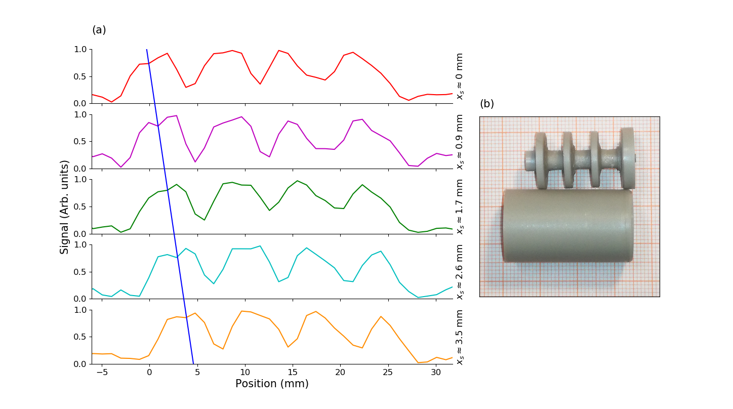
Figure 1: 1-D imaging of a structured (four disks) water sample contained in the plastic cartridge shown in the picture (b). The plots (a) represent MRI profiles, as obtained when the sample occupies four different positions $x_{s}$. Both the structure details and the positions (actual $x_{s}$ values are reported the right-side y-axes) are determined with submillimetric precision.

The narrow width of the atomic magnetic resonance can be restored by applying tailored tuning and/or dressing fields. We will consider here the case of single field dressing, where the gradient $G$ makes $\Omega_{\mathrm{L}}$ position-dependent according to

$$\Omega_{\mathrm{L}}(x)=|J_{0}(\xi(x))\omega_{3}(x)|,$$ (12)

where we have considered a position dependent dressing field, making the dressing parameter $\xi$ dependent on $x$, as well.

An appropriate inhomogeneity of $\xi$ makes possible to achieve the condition $\partial\Omega_{L}/\partial x=0$, under which the atomic resonance width is restored. It is worth noting that the nuclear precession is unaffected by the dressing field. The much smaller gyromagnetic factor, makes their dressing parameter vanishing and the effects of $B_{1}$ negligible: the MRI frequency encoding based on $G$ is preserved.

In this configuration, $B_{1}$ is inhomogeneous, and, in a dipole approximation, at a distance $x$ from the cell center, the dressing field $B_{x}$ is

$$B_{x}(x,t)=\frac{\mu_{0}}{2\pi}\frac{m(t)}{(x_{0}+x)^{3}}=B_{1}(x)\cos(\Omega t),$$ (13)

where $\mu_{0}$ is the vacuum permittivity, $m(t)=m_{0}\cos(\Omega t)$ is the oscillating dipole momentum, and $x_{0}$ is the distance of the dipole from the cell center. Taking now into account the dependence on $x$ of both the static and the dressing fields, accordingly with the eq.11, the dressed angular frequency results

$$\Omega_{L}(x)=\frac{\gamma_{\mathrm{Cs}}}{2\pi}\left(B_{0}+Gx\right)J_{0}\left(\frac{\gamma_{\mathrm{Cs}}B_{1}(x)}{\Omega}\right),$$ (14)

or, in a first-order Taylor approximation,

$$\begin{split}\Omega_{\mathrm{L}}(x)=\Omega_{\mathrm{L}}(0)+\Omega_{\mathrm{L}}^{\prime}(0)\,x+O(x^{2})\approx\frac{\gamma_{\mathrm{Cs}}}{2\pi}\left(B_{0}J_{0}(\alpha)+\left[\frac{3B_{0}\alpha J_{1}(\alpha)}{x_{0}}+GJ_{0}(\alpha)\right]x\right),\\ \end{split}$$

where $\alpha=(\mu_{0}/2\pi)(\gamma_{\mathrm{Cs}}m_{0})/(\Omega x_{0}^{3})$. In conclusion, the condition for compensating the effect of the gradient $G$ is found to be:

$$-3\frac{B_{0}}{x_{0}}\frac{\alpha J_{1}(\alpha)}{J_{0}(\alpha)}=G.$$ (15)

This shows that with an appropriate choice of $\alpha$, the width of the atomic magnetic resonance is substantially restored, as to recover the magnetometer performance to a level making it suited to detect weak MRI signals.

The Figure 1 shows MRI profiles obtained with this methodology. The frequency encoding is here obtained with a field gradient $G\approx 100$nT/cm. The presence of $G$ broadens the atomic MR from its original 25 Hz up to about 800 Hz. Its width is then restored down to 35 Hz by inhomogeneous dressing.

4 Tuning-dressing experiment

The Eq.11 expresses the dependence of dressed angular frequency $\Omega_{\mathrm{L}}$ on the experimental parameters (strengths, relative phase and frequencies of the tuning and dressing fields). The predicted behaviour is verified using the mentioned Bell and Bloom magnetometer. Measurements are made with $p=1,2,3$, and $\Omega_{\mathrm{L}}$ is recorded as a function of $\omega_{1}$ and $\phi$.

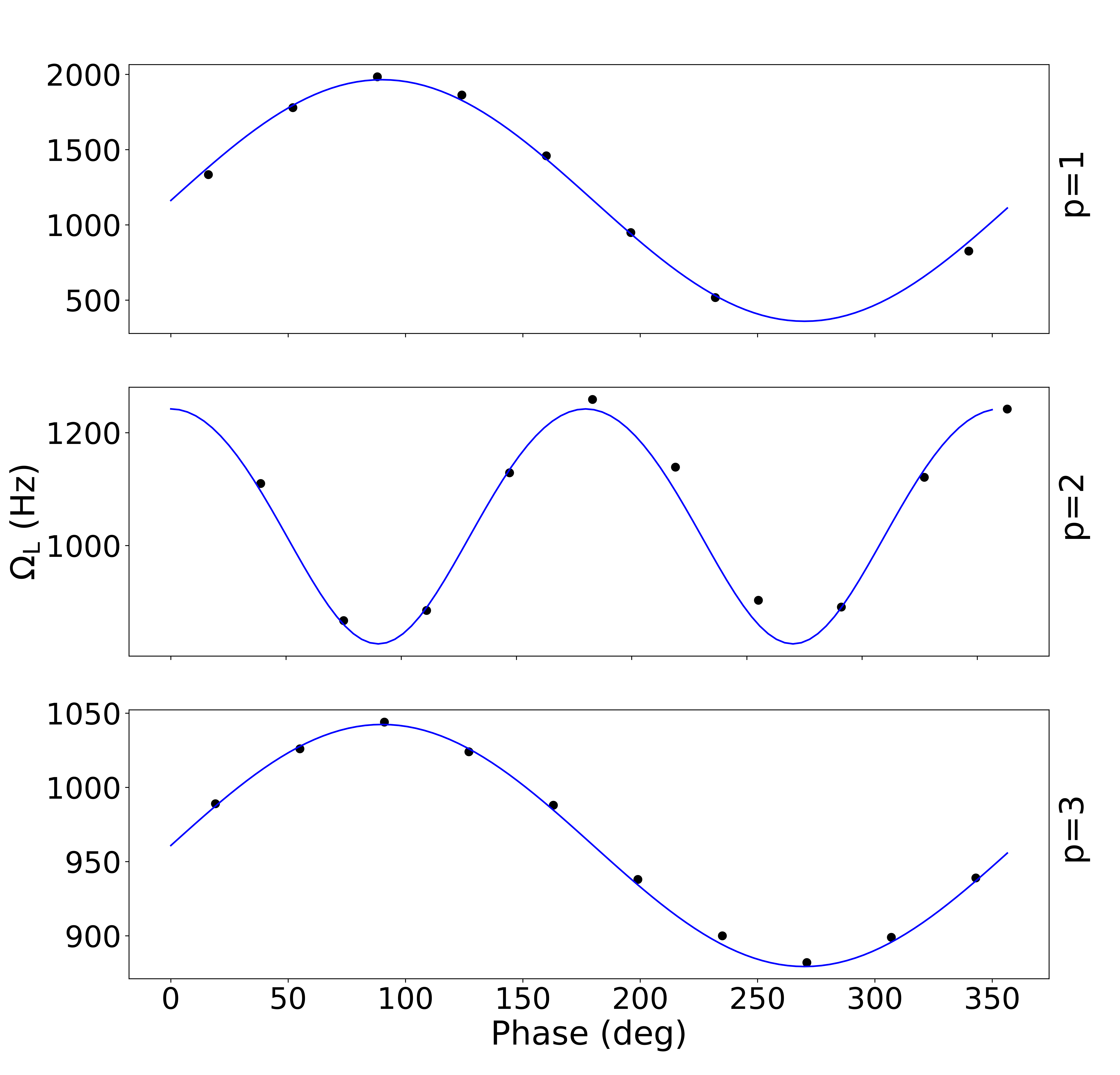
(a)

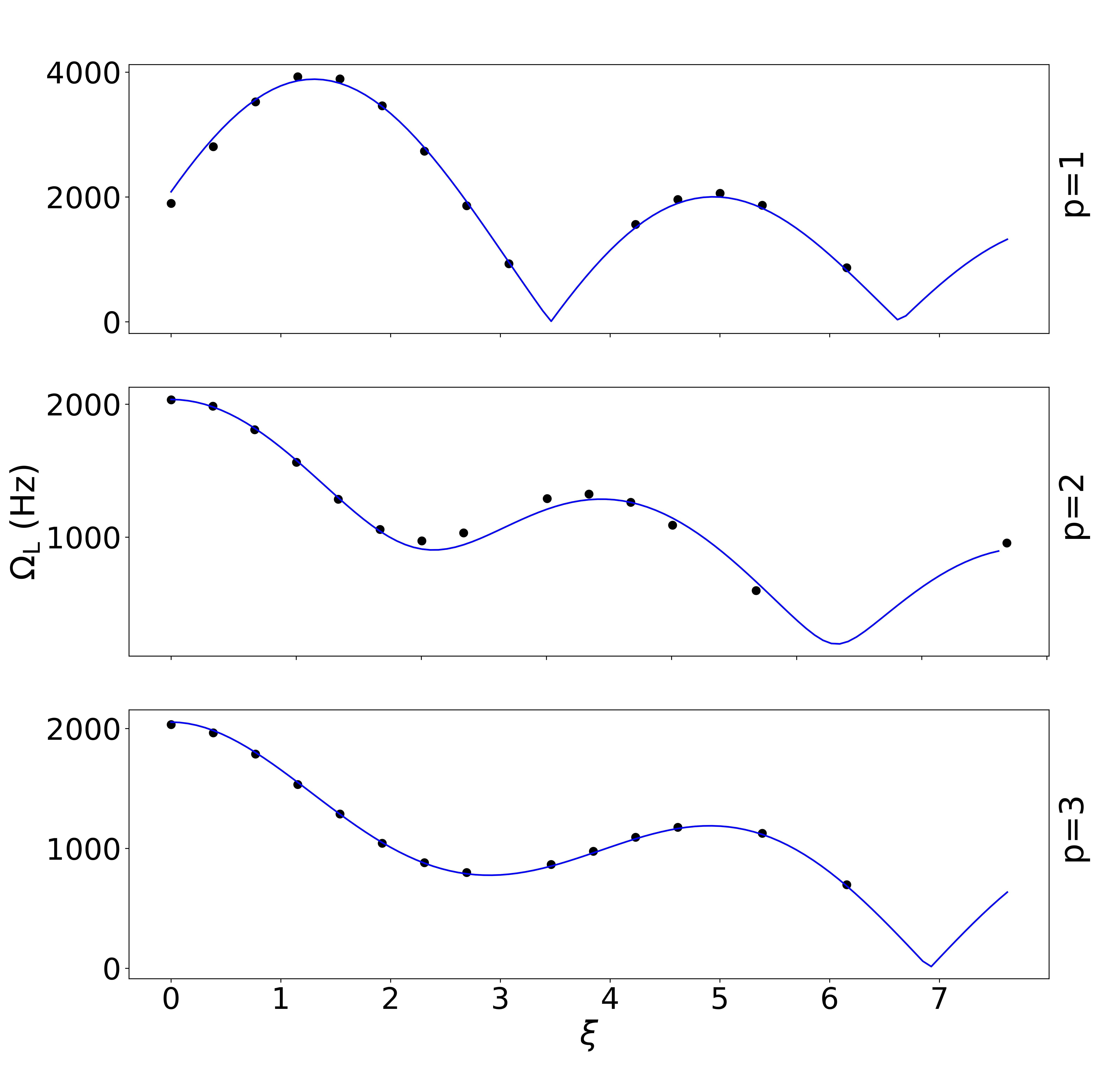
(b)

Figure 2: (a) $\Omega_{\mathrm{L}}$ as a function of the relative phase $\phi$ between the fields $B_{1}$ and $B_{2}$. In black dots the experimental measurements, in blue the theoretical predictions. Upper, middle and bottom panels refer respectively to the cases with $p=1,2,3$, in which $\xi$ has been fixed to $1.38,3.83,1.54$. (b) $\Omega_{\mathrm{L}}$ as a function of the Bessel functions argument $\xi$. In black dots the experimental measurements, in blue the theoretical predictions. Upper, middle and bottom panels refer respectively to the cases with $p=1,2,3$. In the cases with an odd $p$ the phase between $B_{1}$ and $B_{2}$ is fixed to $\phi=\pi/2$, when $p$ is even the phase $\phi$ is set to zero. In each plot, $\xi$ changes varying the value of $B_{1}$, which ranges from zero to $\approx 15\ \mu$T.

Figure 2 shows comparisons of measured and calculated values of $\Omega_{\mathrm{L}}$ as a function of $\phi$ for given $\xi$ and as a function of $\xi$ for given $\phi$, respectively. The data shown in Figure 2(b) are measured with the $\phi$ values that maximize the tuning effect. i.e. is $\phi=\pi/2$ for the odd $p$ values and $\phi=0$ for the even one.

There is an excellent accordance between the experimental data and the theoretical prediction. In particular, both the dependence of the relative phase $\phi$ and on the pertinent $J_{p}$ (with $p=1,2,3$) Bessel functions are perfectly verified by the experiment. Minor deviations can be attributed to experimental imperfections, mainly to not-exact perpendicularity of the applied fields $B_{1}$ and $B_{2}$.

The developed model and its excellent correspondence with the experimental results demonstrates the possibility to enhance the control of spins evolution by means of the described tuning-dressing field arrangement.

This enhancement opens up to a variety of new experimental configurations in which the new set of parameters ($B_{2}$, $p$ and $\phi$) add to $B_{1}$ and $\Omega$ to make new handles available to finely control the atomic magnetization dynamics. Compared to the known cases of harmonic [1] or anharmonic [10] dressing field oscillating along one direction, noticeably here the dressed frequency $\Omega_{\mathrm{L}}$ (eq.11) may exceed $\omega_{3}$.

The tuning-dressing scheme makes possible to chose a parameter set to achieve an arbitrary $d\Omega_{\mathrm{L}}/d\xi$ in conjunction with an arbitrary (to some extent) value of $\Omega_{\mathrm{L}}$. For instance, it is possible to produce a condition of critical dressing (equalization of precession frequencies of different species) [17, 9] with no first-order dependence on $\xi$, so to attenuate the detrimental effects caused by $B_{1}$ inhomogeneities, which constitute a severe limiting problem in high-resolution experiments [9].

Similarly, it is possible to fulfill the condition of a large $d\Omega_{\mathrm{L}}/d\xi$ avoiding the constraint of a strong $\Omega_{\mathrm{L}}$ reduction. The latter may help in applications like that described in Sec.3, where $\Omega_{\mathrm{L}}$ is made deliberately position-dependent by means of a spatially inhomogeneous $\xi$. In addition, for that kind of application, it is worth noting that the presented scheme makes it possible to render $\Omega_{\mathrm{L}}$ space dependent by means of an inhomogeneity of the field $B_{2}$, which is of easier implementation and control, being $B_{2}\ll B_{1}$.

Other applications where the tuning-dressing scheme may offer important potentials is suggested by the dependence on $\phi$. As recently reported [18], an emerging application of highly sensitive magnetometers concerns the detection of targets made of weakly conductive materials. In that case, the typical setup is based on a radio-frequency magnetometer, where the target modifies the amplitude or the phase of a (resonant) radio-frequency field driving the magnetometer. Alternative setups could be developed, where the target modifies the field $B_{2}$, whose frequency is not required to match the atomic resonance. In this case, provided that $J_{p}(\xi)$ is large (e.g. $\xi\approx 1.84$ in the case of $p=1$), the system would have a large response to any variation of either the amplitude (if $\phi=\pm\pi/2$) or the phase (if $\phi=0,\pi$) of $B_{2}$ caused by eddy currents induced in the target.

Appendix A Appendix

The explicit expressions for the matrices in the main text are

$$A_{1}=\begin{pmatrix}0&0&0\\ 0&0&-1\\ 0&1&0\end{pmatrix}\,,\,\,A_{2}=\begin{pmatrix}0&0&1\\ 0&0&0\\ -1&0&0\end{pmatrix}\,,\,\,A_{3}=\begin{pmatrix}0&1&0\\ -1&0&0\\ 0&0&0\end{pmatrix}$$ (16)

Defining $L_{j}=iA_{j}$ and taking the base that diagonalizes $L_{3}$ one obtains the familiar form for the angular momentum operators acting on the $|L=1,M_{L}\rangle$ states. This demonstrates that the algebra generated by the $A_{i}$ matrices is the same of the quantum angular momentum operators. Moreover, it is straightforward to demonstrate that the quantum mean value $\langle\gamma\mathbf{L}\rangle$ satisfies the same classical Larmor equation.

The action of a general antisymmetric matrix $W=a_{1}A_{1}+a_{2}A_{2}+a_{3}A_{3}$ on a given vector $\mathbf{v}$ is the cross-product

$$W\mathbf{v}=\mathbf{a}\times\mathbf{v}\qquad\mathbf{a}\equiv(a_{1},a_{2},a_{3}).$$ (17)

Using the Cayley-Hamilton theorem, the needed matrix exponentials can be analytically evaluated. Let write $\mathbf{a}=\theta\mathbf{\hat{a}}$ with $\mathbf{\hat{a}}\cdot\mathbf{\hat{a}}=1$ then

$$\e^{W}\mathbf{v}=\sum_{n=0}^{+\infty}\frac{W^{n}}{n!}\mathbf{v}=\mathbf{v}+\sin\theta\,\mathbf{\hat{a}}\times\mathbf{v}+(1-\cos\theta)\,\mathbf{\hat{a}}\times(\mathbf{\hat{a}}\times\mathbf{v}).$$ (18)

The auxiliary $f_{i}$ functions introduced in the main text are defined as

$$f_{1}(\tau) =\sum_{n=1}^{\infty}\frac{J_{2n}(\xi)}{n}\sin(2n\tau)$$ (19)

$$f_{2}(\tau) =4\sum_{n=0}^{\infty}\frac{J_{2n+1}(\xi)}{2n+1}\sin^{2}((n+1/2)\tau)$$ (20)

$$f_{3}(\tau) =\Re(g(\tau))$$ (21)

$$f_{4}(\tau) =\Im(g(\tau))$$ (22)

where

$$g(\tau)=\e^{i\phi}\sum_{n\neq-p}\frac{J_{n}(\xi)}{i(n+p)}\left(\e^{i(n+p)\tau}-1\right)+\e^{-i\phi}\sum_{n\neq p}\frac{J_{n}(\xi)}{i(n-p)}\left(\e^{i(n-p)\tau}-1\right)$$ (23)

These functions have a limited and oscillating behaviour and are needed in the evaluation of $\e^{\Lambda_{1}(\tau)}$. One can see by inspection that $\e^{\Lambda_{1}}\approx\mathbbmss{1}$ is a good approximation.

The initial condition appropriate for the experiment is $\mathbf{M}(0)\propto(1,0,0)$ and the quantity monitored is $M_{x}(\tau)$. So applying eq. (18) to evaluate $\e^{\tau F_{1}}$, and then eq. (3), one finds

$$M_{x}(t)\propto\cos(\Omega_{\mathrm{L}}\;t).$$ (24)

References

References

- [1] Haroche S, Cohen-Tannoudji C, Audoin C and Schermann J P 1970 Phys. Rev. Lett. 24 861–864
- [2] Yabuzaki T, Tsukada N and Ogawa T 1972 Journal of the Physical Society of Japan 32 1069–1077
- [3] Kunitomo M and Hashi T 1972 Physics Letters A 40 75–76
- [4] Ito H, Ito T and Yabuzaki T 1994 Journal of the Physical Society of Japan 63 1337
- [5] Holthaus M 2001 Phys. Rev. Applied 64 011601
- [6] Gerbier F, Widera A, Fölling S, Mandel O and Bloch I 2006 Phys. Rev. A 73(4) 041602 URL https://link.aps.org/doi/10.1103/PhysRevA.73.041602
- [7] Hofferberth S, Fischer B, Schumm T, Schmiedmayer J and Lesanovsky I 2007 Physical Review A - Atomic, Molecular, and Optical Physics 76 013401
- [8] Pervishko A A, Kibis O V, Morina S and Shelykh I A 2015 Phys. Rev. B 92(20) 205403 URL https://link.aps.org/doi/10.1103/PhysRevB.92.205403
- [9] Swank C M, Webb E K, Liu X and Filippone B W 2018 Phys. Rev. A 98(5) 053414 URL https://link.aps.org/doi/10.1103/PhysRevA.98.053414
- [10] Bevilacqua G, Biancalana V, Dancheva Y and Moi L 2012 Phys. Rev. A 85 042510 (Preprint 1112.1309)
- [11] Bevilacqua G, Biancalana V, Dancheva Y and Vigilante A 2019 Phys. Rev. Applied 11(2) 024049 URL https://link.aps.org/doi/10.1103/PhysRevApplied.11.024049
- [12] Bevilacqua G, Biancalana V, Dancheva Y and Vigilante A 2019 Appl.Phys.Lett. 115 174102 (Preprint https://arxiv.org/abs/1908.01283) URL https://doi.org/10.1063/1.5123653
- [13] Bevilacqua G, Biancalana V, Vigilante A, Zanon-Willette T and Arimondo E 2020 Phys. Rev. Lett. 125(9) 093203 URL https://link.aps.org/doi/10.1103/PhysRevLett.125.093203
- [14] Bell W E and Bloom A L 1957 Phys. Rev. 107(6) 1559–1565 URL https://link.aps.org/doi/10.1103/PhysRev.107.1559
- [15] Blanes S, Casas F, Oteo J and Ros J 2009 Physics Reports 470 151 – 238 ISSN 0370-1573 URL http://www.sciencedirect.com/science/article/pii/S0370157308004092
- [16] Bevilacqua G, Biancalana V, Chessa P and Dancheva Y 2016 Applied Physics B 122 103 ISSN 1432-0649 URL http://dx.doi.org/10.1007/s00340-016-6375-2
- [17] Golub R and Lamoreaux S K 1994 Physics Reports 237 1 – 62 ISSN 0370-1573 URL http://www.sciencedirect.com/science/article/pii/0370157394900841
- [18] Marmugi L, Deans C and Renzoni F 2019 Applied Physics Letters 115 083503 (Preprint https://doi.org/10.1063/1.5116811) URL https://doi.org/10.1063/1.5116811