Larmor frequency dressing by a non-harmonic transverse magnetic field

Abstract

We present a theoretical and experimental study of spin precession in the presence of both a static and an orthogonal oscillating magnetic field, which is non-resonant, not harmonically related to the Larmor precession and of arbitrary strength. Due to the intrinsic non-linearity of the system, previous models that account only for the simple sinusoidal case cannot be applied. We suggest an alternative approach and develop a model that closely agrees with experimental data produced by an optical-pumping atomic magnetometer. We demonstrate that an appropriately designed non-harmonic field makes it possible to extract a linear response to a weak dc transverse field, despite the scalar nature of the magnetometer, which normally causes a much weaker, second-order response.

I Introduction

The precession of spins in a static homogeneous field is a well known problem of classic as well as quantum physics. A second widely studied system is derived from the previous one when an oscillating field perpendicular to the static one is added. This is the configuration used in typical magnetic resonance (MR) experiments, and for this reason, it has been extensively studied. In MR setups, however, the transverse field oscillates at a frequency near-resonant to the Larmor frequency set by the static field, and has usually an amplitude much smaller than the static one. The resonant condition greatly facilitates the task of modeling the system: the oscillating field is seen as a superposition of two counter-rotating (and usually weak) fields, one of which appears to be (quasi-) static in a reference frame which rotates at the Larmor frequency around the static field, while the other has negligible effects. This is well-known in textbooks as the rotating wave approximation (RWA).

In this work we study the system described above, but in conditions which make the RWA unsuitable. In particular, we consider the cases in which the transverse field has a general periodic time dependence containing Fourier components at frequencies much larger than the Larmor frequency. In fact, we re-examine, extend, and generalize the results reported decades ago by S.Haroche and co-workers Haroche et al. (1970), where similarly an analytical model has been developed and applied to interpret experimental data from optical detection of atomic precession.

The results presented here are modeled with the Larmor equation and discussed using a perturbative approach based on the Magnus expansion of the time-development operator. Compared to previous works on this subject, our approach makes it easy to model the effects of a transverse field oscillating with an arbitrary waveform.

It seems worth stressing that the subject has implications for the research area of dynamic localization Kenkre and Raghavan (2000); Holthaus and Hone (1996), which concerns the effect of a time-periodic field on quantum systems such as charged particles in crystals Dunlap and Kenkre (1986) and Bose Einstein condensates Eckardt et al. (2009).

The experimental implementation is feasible, provided that a slow precession occurs around a weak static field, for instance with ultra-low-field NMR setups and in atomic spin precession experiments. This latter is the nature of the setup used in our case, and the reported experimental results concern measurements performed with an optical-pumping atomic magnetometer operated at a $\mu$T static field range. The corresponding Larmor frequency is in the kHz range, making it easy to apply a homogeneous transverse field oscillating at much higher frequencies, even with a much larger amplitude.

Our apparatus detects the time-dependent Faraday rotation of the polarization plane of a weak probe laser beam, which is directly related to a component of the macroscopic magnetization of atoms. The analyzed magnetization component is the one parallel to the direction of the oscillating field, which coincides with the probe beam propagation axis. In the presence of a strong transverse oscillating field the three components of the magnetization evolve in time with a complex behaviour, which is far from a simple precession. Nevertheless the measured component maintains its similarity to the simple precession behaviour. In other terms, the motion around the direction ($z$) of the static field is deeply affected by a strong non-resonantly oscillating field along $x$, which mainly modifies the dynamics of the magnetization components $M_{y}$ and $M_{z}$, but leaves $M_{x}$ evolving (approximately) with a simple harmonic law. This quasi-harmonic evolution of $M_{x}$ makes it possible to define a modified (dressed) Larmor frequency even when the oscillating field is so strong that no precession motion could be recognized by simply observing the time evolution of the whole $\mathbf{M}$ vector.

The paper is organized as follows: in Section II we describe the experimental setup used, in Section III we discuss the theoretical model, and Section IV contains the discussion and the conclusions.

II Experimental setup

The basic structure of the experimental setup is that of an optical atomic magnetometer (see Fig. 1). Using a resonant circularly polarized laser light, alkali atoms are pumped in a specific Zeeman sublevel and thus the medium is magnetized along the wave-vector ($x$) direction. The atomic medium is placed in a homogeneous magnetic field ($z$ direction) transverse to the pump light propagation. Consequently the Zeeman sublevel where atoms are pumped evolves in time, giving rise to the magnetization precession in the $xy$ plane, around the static magnetic field.

This precession is detected by analyzing the Faraday rotation of a weak, linearly polarized, probe beam which propagates in the $xy$ plane (in our case it is collinear to the pump beam). The linear probe beam polarization can be decomposed in two $\sigma^{+}$ and $\sigma^{-}$ counter-rotating circularly polarized components, which experience variation of the respective refractive indexes due to the atomic spin precession. These two circular components recombine with a time-dependent relative dephasing in a linear polarization rotated by an angle oscillating at the Larmor frequency. Beside the different dispersions, the $\sigma^{+}$ and $\sigma^{-}$ components suffer also different absorptions, but this aspect is made of little relevance by tuning the probe laser away from the resonance center.

To contrast the relaxation processes that cause a progressive decay of the induced magnetization, and hence of the detected signal, the pump light is applied periodically, synchronously with the precession of the atomic spins, i.e. resonantly with the Larmor frequency set by the static magnetic field.

In our setup, the pump radiation is generated by a single-mode, distributed feedback, pigtailed DFB diode laser, whose optical frequency is controlled through the junction current and is periodically made resonant (or non resonant) to the D1 transition of Cs, at 894 nm. It illuminates the atomic sample at an intensity of about 0.5 mW/cm². The probe radiation is generated by a single-mode, Fabry-Perot, pig-tailed diode laser resonant with the D2 line of Cs, at 852 nm. It illuminates the sample at much weaker intensity, being attenuated at a level of about half $\mu$W/cm², in order to negligibly perturb the sample.

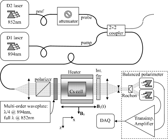
Figure 1: Schematics of the experimental setup. The probe laser is tuned to the D2-Cs line @852nm and unmodulated; the pump laser is tuned to the D1-Cs line @894nm and is modulated synchronously with the atomic precession. Both are mixed and coupled to the sensor though polarization maintaining fibres (pmf). The probe is attenuated down to $\mu$W level before the Cs cell, the pump is stopped by an interferential filter (Int fltr) after the cell. A multi-order waveplate renders the pump polarization circular, while leaving the probe polarization linear. The Cs cell contains 23 Torr of N₂ as a buffer gas, which quenches the fluorescence and slows down the Cs atom motion, making it diffusive. The cell is slightly heated to increase Cs vapour density. The transmitted probe laser polarization is analyzed by a balanced polarimeter made of a Rochon polarizer oriented at $45^{o}$ with respect to the probe polarization axis and two photodiodes. A differential transimpedance amplifier converts the photocurrent to a voltage signal, which is then digitally acquired. That signal reproduces the Faraday rotation, associated to the time-dependent orientation of the precessing atomic spins.

Polarization maintaining (PM) fibres bring the radiation of the two lasers to a coupler (via an on-fibre attenuator in the case of the probe) which mixes them in the PM fibre illuminating the sample. In proximity of the atomic sample, the two radiations emerging from the fibre end are collimated by a lens, their linear polarization is reinforced by a polarizing cube.Then, a phase-plate acts differently on the polarization of both the radiations, rendering the pump radiation circular, while leaving the probe one linear. This double effect is achieved thanks to a multi-order wave plate made of a 480$\mu$m quartz layer, which introduces Ghosh (1999) for the crossed linear polarization components of the two wavelengths a (5+1/4)$\lambda_{D1}$ and a 5$\lambda_{D2}$ relative delays, respectively. Such method of tailored multi-order waveplate method is quite similar to that applied in the magnetometric setup (based on Rb vapors) described in Johnson et al. (2010).

After interacting with the atomic sample, the pump radiation is blocked by an interferential filter and the probe beam polarization is analyzed by a balanced polarimeter made of a 45^o oriented Rochon and a couple of photodetectors whose photocurrent difference is amplified by a low-noise transimpedance amplifier.

The polarimetric signal is either analyzed as a function of the laser-modulation frequency to characterize the atomic magnetic resonance, or used to generate a signal for driving the laser optical frequency, thus closing a loop which makes the system a self-oscillator. In the first case, the precession frequency is estimated with a best fit procedure, while in the second case it is evaluated as the self-oscillation frequency, provided that the loop delay is properly compensated. In practice, the closed-loop, self-oscillating operation helps in shortening the measurement time, but may introduce systematic errors due to inappropriate choice of the loop delay. On the contrary, operating in the open loop/scanned frequency/best fit procedure requires a longer time but improves the accuracy in the Larmor frequency determination. All the plots reported in Sec. IV were obtained in this more accurate open-loop operation mode. With the used static field intensities, the precession frequency ranges from hundreds of Hz to several kHz.

The atomic sample is made of a high quality gas-buffered cell containing a droplet of Cs and 23 Torr of N₂. The buffer gas is suitable for slowing down the thermal motion of Cs atoms, making it diffusive and also quenches any stray fluorescence light. Following several optimization campaigns devoted to improve the sensitivity of the setup in magnetometric applications, the pump laser is made resonant (at the right time) with the $|^{1}S_{1/2},F_{g}=4\rangle\rightarrow|^{1}P_{1/2}\rangle$ hyperfine components of the D1 line, while the analyzed ground state is the $F_{g}=4$ and the detection is made tuning the probe laser about 2  GHz on the blue wing of the line made of the triplet $|^{1}S_{1/2},F_{g}=4\rangle\rightarrow|^{2}P_{3/2}\rangle$. The pump radiation is broadly modulated with a slightly asymmetric signal, so that, besides the synchronous excitation of the $|^{1}S_{1/2},F_{g}=4\rangle$ level, it also spends some time in resonance with the $|^{1}S_{1/2},F_{g}=3\rangle\rightarrow|^{2}P_{3/2}\rangle$ triplet.

The Cs cell is inserted in an anti-inductive heating coil by which the temperature is increased up to about 50^oC in order to reach a good compromise for having a large signal (an optimal optical depth) without introducing an excessive broadening due to the increase of spin-exchange collision rate. A second coaxial, inductive coil makes it possible to apply a homogeneous time dependent transverse field which is thus parallel to the optical axis. This second coil is supplied by a digital waveform generator which provides an arbitrary periodic voltage signal. This signal is designed to produce current (and hence $x$-oriented magnetic field) Fourier components with appropriate phases and amplitudes, in accordance to the measured complex impedance of the coil.

The whole experiment is conducted in a magnetically clean volume, where a set of three mutually perpendicular, large size Helmholtz coils and a set of quadrupoles make it possible to control the three components of the magnetic field and reduce their inhomogeneities. In particular, the horizontal components ($x$, $y$) of the Earth field are fully compensated while the vertical one ($z$), partially compensated down to a few $\mu$T, determines the static field.

The system is here used for an absolute frequency measurement. Nevertheless, the apparatus is designed to perform differential measurements as well. In fact, the fibre coupler is a $2\times 2$ 50% device, meaning that the two radiations are mixed in equal ratios and made available in two output PM fibres. Thus, the apparatus can easily be adapted to work with a dual sensor, suitable for gradiometry and for differential magnetic measurements. The accuracy in the absolute frequency measurement (order of 1 Hz) is largely in excess compared to the needs of this work, and is limited by the environmental magnetic noise.

III Model

The aim of this section is to describe and characterize the precession of spins in the presence of a time dependent magnetic field orthogonally oriented with respect to the static one, using a special form of the perturbation theory for the time evolution operator.

As stated above, taking the $z$ axis in the direction of the static field and the $x$ axis along the alternating one, i.e. $\mathbf{B}=(B_{x}\,\phi(\omega t),0,B_{z})$, the Larmor equations for the magnetization are

$$\begin{cases}\dot{M}_{x}&=-\Omega_{z}M_{y}\\ \dot{M}_{y}&=\Omega_{z}M_{x}-\Omega_{x}{\phi}(\omega t)\,M_{z}\\ \dot{M}_{z}&=\Omega_{x}{\phi}(\omega t)\,M_{y}\end{cases}$$ (1)

Here $\Omega_{x,z}=\gamma B_{x,z}$ ($\gamma$ is the gyromagnetic ratio) and $\phi(\omega t)$ is a real and periodic function with a well-behaved Fourier expansion. Notice that hereafter the magnetization is treated classically, but the same results hold true if the $M_{i},\;i=x,y,z$ are treated as non-commuting quantum mechanical operators.

Using the dimensionless time $\tau=\omega t$, the equation set (1) can be recast as

$$\frac{d}{d\tau}\mathbf{M}=\left[\frac{\Omega_{z}}{\omega}\begin{pmatrix}0&-1&0\\ 1&0&0\\ 0&0&0\end{pmatrix}+\frac{\Omega_{x}}{\omega}\begin{pmatrix}0&0&0\\ 0&0&-1\\ 0&1&0\end{pmatrix}\phi(\tau)\right]\mathbf{M}.$$ (2)

We are interested in the case of $\zeta\equiv\Omega_{z}/\omega\ll 1$, so it is natural to use perturbation theory. To keep track of the perturbation order, we introduce the parameter $\epsilon$ and let $\zeta\rightarrow\epsilon\zeta$ in the intermediate formulas, we set then $\epsilon=1$ at the end of the calculations. We can thus rewrite eq. (2) as

$$\frac{d}{d\tau}\mathbf{M}=\left[\epsilon\,\zeta\,A_{z}+\xi\,\phi(\tau)A_{x}\right]\mathbf{M},$$ (3)

where $\xi\equiv\Omega_{x}/\omega$. Notice that introducing the commutator $A_{y}\equiv[A_{z},A_{x}]$, the three matrices $A_{k},\;k=x,y,z$ constitute essentially the three-dimensional real representation of the angular momentum quantum operators.

The magnetization $\mathbf{M}(\tau)$ can be obtained acting with the time evolution operator $U(\tau)$ as $\mathbf{M}(\tau)=U(\tau)\mathbf{M}(0)$ on the initial value $\mathbf{M}(0)$. In the spirit of perturbation theory, it is useful to factorize $U$ in the “interaction” representation as

$$U(\tau)=\exp\left[\xi\int_{0}^{\tau}\phi(\tau^{\prime})d\tau^{\prime}\,A_{x}\right]\;U_{I}(\tau)=\begin{pmatrix}1&0&0\\ 0&\cos\Phi&-\sin\Phi\\ 0&\sin\Phi&\cos\Phi\end{pmatrix}\;U_{I}(\tau)$$ (4)

which implicitly defines $U_{I}(\tau)$. Moreover we set

$$\Phi(\tau)=\xi\int_{0}^{\tau}\phi(\tau^{\prime})d\tau^{\prime}.$$ (5)

Let’s comment on the structure of eq.(4): the first factor represents a rotation of an angle $\Phi$ around the first axis. This rotation relates the laboratory frame to the rotating frame, thus $\Phi$ is the Larmor angle for the precession around the oscillating field. In the rotating frame, the evolution operator satisfies

$$\frac{dU_{I}}{d\tau}=\epsilon\zeta\mbox{$\mathrm{e}^{-\Phi(\tau)A_{x}}$}A_{z}\mbox{$\mathrm{e}^{\Phi(\tau)A_{x}}$}\;U_{I}=\epsilon\zeta\left[\cos\Phi\,A_{z}+\sin\Phi\,A_{y}\right]\;U_{I}=\epsilon\zeta A_{z}^{(I)}\;U_{I}$$ (6)

whose solution, following the Magnus expansion device Blanes et al. (2009), can be written as

$$U_{I}(\tau)=\mbox{$\mathrm{e}^{W(\tau)}$}.$$ (7)

The exponent satisfies the non-linear equation Blanes et al. (2009)

$$\frac{dW}{d\tau}=\epsilon\zeta\,A_{z}^{(I)}-\frac{1}{2}\left[W,\epsilon\zeta\,A_{z}^{(I)}\right]+\frac{1}{12}\left[W,\left[W,\epsilon\zeta\,A_{z}^{(I)}\right]\right]+\ldots$$ (8)

which can be solved perturbatively. In fact expanding $W$ as $W=\sum_{n\geq 1}\epsilon^{n}\,W_{n}$ one gets the first order contribution

$$W_{1}(\tau)=\zeta\,\mathrm{Re}(\Psi(\tau))\,A_{z}+\zeta\,\mathrm{Im}(\Psi(\tau))\,A_{y}$$ (9)

where we introduced the quantity

$$|\Psi(\tau)|\mbox{$\mathrm{e}^{i\beta(\tau)}$}=\int_{0}^{\tau}\mbox{$\mathrm{e}^{i\,\Phi(\tau^{\prime})}$}\,\mathrm{d}\tau^{\prime}.$$ (10)

After some algebra one finds

$$U_{I}=\begin{pmatrix}\cos(\zeta|\Psi|)&-\cos\beta\,\sin(\zeta|\Psi|)&\sin\beta\,\sin(\zeta|\Psi|)\\ \cos\beta\,\sin(\zeta|\Psi|)&\cos^{2}\beta\cos(\zeta|\Psi|)+\sin^{2}\beta&\sin(2\beta)\sin^{2}(\zeta|\Psi|/2)\\ -\sin\beta\,\sin(\zeta|\Psi|)&\sin(2\beta)\sin^{2}(\zeta|\Psi|/2)&\sin^{2}\beta\cos(\zeta|\Psi|)+\cos^{2}\beta\end{pmatrix}$$ (11)

which represents a rotation of an angle $\zeta|\Psi|$ around the axis

$$\mathbf{n}=\begin{pmatrix}0,&\sin\beta,&\cos\beta\end{pmatrix}.$$ (12)

Considering the initial magnetization prepared along the $x$ axis $\mathbf{M}(0)=\left(M_{x}(0),0,0\right)$ and using the eqs. (11) and (4) one finds

$$M_{x}(\tau)=M_{x}(0)\,\cos(\zeta|\Psi(\tau)|),$$ (13)

clarifying that $\Psi$ is the Larmor angle around the axis $\mathbf{n}$. Deriving this quantity, the first-order correct frequency of the signal experimentally analyzed can be evaluated

$$\Omega^{(1)}_{L}=\omega\frac{d}{d\tau}\,\left(\zeta|\Psi(\tau)|\right).$$ (14)

Notice that, on general ground, if one needs only the argument of the cosine in (13), it can be more easily obtained by calculating the eigenvalues of $W_{1}$.

Another case of practical interest is the following

$$\frac{d}{d\tau}\mathbf{M}=\left[\epsilon\,\zeta\,A_{z}+\epsilon^{2}\,\xi_{0}\,A_{x}+\xi\,\phi(\tau)A_{x}\right]\mathbf{M},$$ (15)

which models the case of a very small (residual) static magnetic field superimposed to the alternating one. Precisely we assume that the dimensionless quantities $\xi$, $\zeta$ and $\xi_{0}$ satisfy

$$\xi\equiv\gamma B_{x}^{\mathrm{(ac)}}/\omega\approx O(1)\qquad\zeta\equiv\epsilon\,\gamma B_{z}/\omega\ll 1\qquad\xi_{0}\equiv\epsilon^{2}\,\gamma B_{x}^{\mathrm{(dc)}}/\omega\ll\zeta,$$ (16)

showing the need of second-order perturbation theory to study the effect of $\xi_{0}$. Repeating the above derivation we get the same $W_{1}$ while the second-order contribution $W_{2}$ becomes

$$W_{2}(\tau)=\left[\xi_{0}\tau-\frac{\zeta^{2}}{2}\mathrm{Im}\int_{0}^{\tau}\Psi(\tau^{\prime})\mbox{$\mathrm{e}^{-i\Phi(\tau^{\prime})\mathrm{d}\tau^{\prime}}$}\right]A_{x}\equiv\chi(\tau)\,A_{x}.$$ (17)

The geometric meaning of $\chi$ is that in the second order approximation the rotation described in eq. (9) does not occur around $\mathbf{n}$, but around a direction having also a small $x$ component. Finding the eigenvalues of $\epsilon\,W_{1}+\epsilon^{2}W_{2}$ makes it possible to determine the argument of the cosine

$$\Theta_{L}(\tau)=\epsilon\sqrt{\zeta^{2}|\Psi(\tau)|^{2}+\epsilon^{2}\,\chi(\tau)^{2}}$$ (18)

and thus eq. (14) generalizes to

$$\Omega^{(2)}_{L}=\omega\frac{d\Theta_{L}(\tau)}{d\tau}.$$ (19)

III.1 Determination of $\Psi$ and $\chi$

We are interested in periodic signals, so that $\phi(\tau)$, $\Phi(\tau)$ and $\exp(i\Phi)$ have a well behaved Fourier expansion. More precisely we consider signals $\phi(\tau)$ with a zero mean so that

$$\mbox{$\mathrm{e}^{i\,\Phi(\tau)}$}=\sum_{n=-\infty}^{\infty}G_{n}\mbox{$\mathrm{e}^{i\,n\,\tau}$}=\sum_{n=-\infty}^{\infty}|G_{n}|\mbox{$\mathrm{e}^{i(\,n\,\tau+\theta_{n})}$},$$ (20)

then it is easy to obtain

$$\int_{0}^{\tau}\mbox{$\mathrm{e}^{i\,\Phi(\tau^{\prime})}$}\mathrm{d}\tau^{\prime}=G_{0}\tau+\sum_{n\neq 0}\frac{G_{n}}{in}\left(\mbox{$\mathrm{e}^{i\,n\,\tau}$}-1\right)=G_{0}\tau+g(\tau).$$ (21)

where the implicitly defined function $g(\tau)$ is a limited and oscillating function. When $\tau\gg 1$ (or $t\gg 1/\omega$) we can neglect $g(\tau)$ obtaining $\Psi(\tau)=G_{0}\tau$, and thus we find a dressed Larmor frequency

$$\Omega^{(1)}_{L}=\Omega_{z}\left|G_{0}\right|.$$ (22)

To access the second-order corrections we need the integral

$$\int_{0}^{\tau}\Psi(\tau^{\prime})\mbox{$\mathrm{e}^{-i\,\Phi(\tau^{\prime})}$}\mathrm{d}\tau^{\prime}=|G_{0}|^{2}\tau^{2}/2+\tau i(a-b)+f_{0}(\tau)+\tau f_{1}(\tau)$$ (23)

where $f_{0}(\tau)$ and $f_{1}(\tau)$ are periodic and limited functions whose explicit form is not important here. The parameters $a$ and $b$ are defined as

$$a\equiv\sum_{n\neq 0}\frac{G_{0}^{*}G_{n}}{n}\qquad b\equiv\sum_{n\neq 0}\frac{|G_{n}|^{2}}{n}.$$ (24)

Neglecting the oscillating terms in eq. (23) as before and taking the imaginary part we get

$$\chi(\tau)=\tau\left[\xi_{0}+\zeta^{2}\left(b-\mathrm{Re}(a)\right)/2\right]\equiv\tau\left(\xi_{0}+\zeta^{2}c/2\right)\equiv\tau\chi_{0}.$$ (25)

The dressed Larmor frequency eq. (19) can thus be evaluated approximating the square root in eq. (18) as

$$\frac{\Omega^{(2)}_{L}}{\Omega_{z}}\approx|G_{0}|\left[1+\frac{\chi_{0}^{2}}{2\zeta^{2}|G_{0}|^{2}}\right]=|G_{0}|+\frac{1}{2|G_{0}|}\left[(\xi_{0}/\zeta)^{2}+\xi_{0}c+\zeta^{2}c^{2}/4\right],$$ (26)

where now we can consider the last terms as corrections to the first-order result (22). Notice how the coefficients $G_{n},\;\,n\neq 0$ are encoded in the $c$ parameter.

III.2 Pure sinusoidal signal

This case has already been studied and reported in literature. S. Haroche et al., in a pioneer paper had already demonstrated the possibility of solving the simple case of a harmonic transverse field  Haroche et al. (1970) with a different approach based on quantum mechanics. In that study, the authors quantized the oscillating field as a bosonic mode (rf photons) and used standard first-order perturbation theory to evaluate the energy shifts. Then, in the (semi-classical) limit of a large boson number, they obtained the same result reported here below. That method would run into difficulties for generic time-periodic signals. On the other hand, let us examine how quickly the results are obtained using our approach. Starting from $\phi(\tau)=\cos\tau$ we easily get $\Phi(\tau)=\xi\sin\tau$ and the coefficients $G_{n}$ are the Bessel functions Abramowitz and Stegun (1964)

$$G_{n}=\left|J_{n}\left(\xi\right)\right|\mbox{$\mathrm{e}^{i\theta_{n}}$}$$ (27)

being the phases $\theta_{n}$ either $0$ or $\pi$ according to the sign of $J_{n}$. We thus re-obtain the Haroche et al. result

$$\Omega_{L}=\Omega_{z}\,\left|J_{0}\left(\xi\right)\right|.$$ (28)

Notice that in case of a general harmonic signal $\phi(\tau)=\cos(\tau-\tau_{0})$ one has

$$\Phi(\tau)=\xi\left[\sin(\tau-\tau_{0})+\sin\tau_{0}\right]$$ (29)

and thus

$$G_{n}=\mbox{$\mathrm{e}^{i\,\xi\sin\tau_{0}}$}\,\left|J_{n}\left(\xi\right)\right|\mbox{$\mathrm{e}^{i(\theta_{n}-n\tau_{0})}$}$$ (30)

giving for $|G_{0}|$ the same result as before.

III.3 Non-harmonic signals

Having found the general expression (22) for the dressed Larmor frequency, we can study more complicated cases. Let’s first introduce a higher harmonic component in the signal, indicating with $r$ the ratio between its amplitude and the fundamental one i.e.

$$\phi(\tau)=\cos\tau+r\cos(k\tau+\varphi)$$ (31)

which gives

$$\Phi(\tau)=\xi\left[\sin\tau+\frac{r}{k}\left(\sin(k\tau+\varphi)-\sin\varphi\right)\right].$$ (32)

Repeating the same steps as before, one gets

$$G_{n}=\mbox{$\mathrm{e}^{-i\,(\xi r/k)\sin\varphi}$}\,\sum_{p=-\infty}^{+\infty}J_{n-kp}\left(\xi\right)\,J_{p}\left(\xi\,r/k\right)\,\mbox{$\mathrm{e}^{i\,p\,\varphi}$}$$ (33)

which is a generalized Bessel function Dattoli and Torre (1996). Thus the leading contribution (eq. (22) ) of the Larmor frequency becomes

$$\frac{\Omega_{L}}{\Omega_{z}}=F(\xi,r,k,\varphi)\equiv\left|\sum_{p=-\infty}^{+\infty}J_{-kp}\left(\xi\right)\,J_{p}\left(\xi\,r/k\right)\,\mbox{$\mathrm{e}^{i\,p\,\varphi}$}\right|.$$ (34)

Another highly non-harmonic signal which gives analytical results is the square wave

$$\Phi(\tau)=\xi\begin{cases}\tau&0\leq\tau\leq 2\pi\alpha\\ \alpha(2\pi-\tau)/(1-\alpha)&2\pi\alpha<\tau<2\pi\end{cases}.$$ (35)

In fact in this case the integration outlined in eq. (20) can be done trivially obtaining

$$G_{0}=\mbox{$\mathrm{e}^{i\pi\xi\alpha}$}\,\frac{\sin(\pi\xi\alpha)}{\pi\xi\alpha},$$ (36)

and thus the dressed Larmor frequency results

$$\frac{\Omega_{L}}{\Omega_{z}}=\frac{|\sin\pi\xi\alpha|}{\pi\xi\alpha}.$$ (37)

For general periodic signals the $G_{n}$ coefficients can be obtained analytically as multiple sums of products of ordinary Bessel functions. However, this approach soon becomes cumbersome and a numerical evaluation of the $G_{n}$, using for instance the Fast Fourier Transform, is a viable alternative.

IV Discussion

The main issue of the paper is to study the effect of an alternating, non-resonant magnetic field oriented perpendicularly to the static one causing a reduction of the precession rate of spins. Such a reduction has a non-monotone dependence on the amplitude of the alternating field, and, under specific conditions, the precession frequency can take a zero value. This phenomenon has been previously observed and theoretically interpreted in the case of a harmonic signal Haroche et al. (1970).

The model introduced in this work is suitable to the description of the simple case of a harmonically oscillating field but also makes it possible to easily extend the analysis to the non-harmonic case.

The comparison of theoretical predictions and experimental results is made taking into account several operating conditions and varying different parameters. We preliminarily test the consistency with known results obtained in the simple case of a transverse field oscillating with a harmonic law. Then we test the strongly non-harmonic case of a square-wave field. A more detailed analysis is presented for the case of a two-Fourier-component field, where we analyse the effect as a function of the amplitudes and of the relative phase of the two components. We also devote attention to the cases when the frequency ratio is even ($k=2$) or odd ($k=3$), pointing out the symmetries discussed in the appendix A. Finally we demonstrate the existence of a linear response to a weak dc field, which has implications in the design of atomic magnetometers with vectorial response.

We show in Fig. 2 the comparison of experimental data obtained with the apparatus described in Sec. II and the curve (namely $\left|J_{0}\right|$) given by the model in the case of a harmonic field. In this figure (as in the following ones) the amplitude of the oscillating field is expressed in terms of the dimensionless quantity $\xi$ defined (see also Sec. III eq. (3)) by $\xi=\Omega_{x}/\omega=\gamma B_{x}/\omega$. The frequency reduction effect is also given in natural dimensionless units, reporting the ratio between the dressed and the unperturbed precession frequencies. It is worth noticing that if the same curves are plotted in terms absolute quantities (i.e. plotting the dressed precession frequency as a function of $B_{x}$), passing from a spinning species to another having a larger gyromagnetic factor, the vertical axis scales up while the horizontal one scales down. This makes it possible to identify conditions for matching the dressed precession frequencies of different species, which is of great interest for possible applications, see for example Ito et al. (2003) and references therein.

Figure 2: Ratio between the dressed and unperturbed precession frequency as a function of the amplitude of the oscillating field (expressed in the dimensionless quantity $\xi=\gamma B_{x}/\omega$) in the case of a harmonic transverse field, according to eq. (28) the plot reproduces the behaviour of $\left|J_{0}\left(\xi\right)\right|$.

As a first example of a non-harmonic modulation, we consider the case of a symmetric (50% duty cycle) square wave. In this case the model predicts a behaviour given by a sinc modulus (eq. (35)). The prediction is in good agreement with the experimental observation, as appears evident in Fig. 3.

Figure 3: Comparison of theoretical predictions (line) and experimental points for the ratio between the dressed and unperturbed precession frequency as a function of the amplitude of a square-wave like oscillating field. According to eq. (37) the behaviour is described by the modulus of a sinc function.

A detailed analysis is performed in the case of a non-harmonic periodic transverse field made of only two Fourier components (a fundamental one plus its $k^{th}$ harmonics). In this case the prediction (see eq. (34)) can be easily compared to the experimental results when varying one of the independent variables, as in the following. In Fig. 4 we preliminarily show the behaviour of $F$ as a function of the amplitude $\xi$ of the fundamental Fourier component and the relative amplitude $r$ (see eq. (31) for the precise meaning of $r$, $k$ and $\varphi$) of the $k^{th}$ harmonics, for fixed values of their relative phase and of $k$.

Figure 4: Graphs of the function $F(\xi,r,k,\varphi)$, see eq. (34), for different values of $k$ and $\varphi$.

Due to technical limitations, only a few lobes of the ones shown in Fig. 4 have been accessed to compare the model prediction with the experimental results. As an example, in Fig. 5 the dependence of $F$ on the amplitude ratio $r$ is presented for several couples $(k,\xi)$ of the frequency ratio and of the fundamental amplitude.

Figure 5: Comparison of theoretical predictions (line) and experimental points for different values of $\xi$ and $k$ as a function of $r$ (see eq. (31)).

One fact which stands out among the most interesting features of the system considered is that the non-linear nature of the observed phenomenon makes relevant the relative phase of the Fourier components of the oscillating field. Figs. 6 and 7 are devoted to comparing the dependency of $F$ on one of those parameters. For a large enough amplitude of both the components, phase values exist causing the precession frequency to vanish.

Figure 6: Comparison of theoretical predictions (line) and experimental points for $k=3$, $\xi=3$ and two values of and $r$ for the ratio between the dressed and unperturbed precession frequencies as a function of the relative phase between the two Fourier components of the oscillating field (see eq. (31)).

Figure 7: Comparison of theoretical predictions (line) and experimental points for $k=2$ and different values of $\xi$ and $r$ for the ratio between the dressed and unperturbed precession frequencies as a function of the relative phase between the two Fourier components of the oscillating field (see eq. (31)).

Two comparisons for $k=3$ are made in Fig. 6, where differently located zeroes and local maxima of $F$ appear. It is worth noting that, as confirmed by the experiment, in the case of $k=3$ the dependence of the relative phase is symmetric with respect to the $\varphi=\pi$ value.

Fig. 7 reports further comparisons made for $k=2$. In these cases due to the small value of $r$, the interference-like pattern does not produce zeroes, while the number of local maxima is clearly dependent on the absolute amplitude $\xi$. For this value of $k$, both the model and the experiment show that the dependence of the relative phase has an additional symmetry with respect to the $\varphi=\pi/2$ value.

The symmetries pointed out in the Figs. 6 and 7, can be interpreted in terms of properties of the Bessel function, according to the analysis presented in brief in the Appendix A. As shown in that appendix, the symmetry around the $\pi$ value is a consequence of a $2\pi$ periodicity occurring for both odd and even values of $k$, while the additional symmetry around $\pi/2$ occurs only for the even values of $k$.

The even-$k$ symmetry can be broken by the presence of a vectorial perturbation along the oscillation axis. In particular, a weak static magnetic field component added to the alternating one results in an asymmetric curve

$$w_{0}\equiv\frac{\Omega_{L}}{\Omega_{z}}\bigg{|}_{\varphi=0}\neq\frac{\Omega_{L}}{\Omega_{z}}\bigg{|}_{\varphi=\pi}\equiv w_{\pi}$$ (38)

as can be seen in Fig. 8, where it is also shown the theoretical simulations with and without the second order corrections (see eq. (26)). A look at the right panel reveals the importance of the corrections depending of the $G_{n}\,,\,n\neq 0$ coefficients through the $c$ quantity (see eq. (25)) in generating the asymmetry.

This asymmetry has potential applications in designing and setting up apparatuses like the magnetometer used in our experiment. The scalar nature of our magnetometer makes it very sensitive to variations of the field component parallel to the static one ($z$ component), while the transverse components can be detected and minimized with procedures responding to the second order in $\xi_{0}$. In contrast, repeated measurements and equalization of $w_{0}$ and $w_{\pi}$ constitute an effective procedure with a first order response in $\xi_{0}$ (see eq. (26)) for fine balancing the transverse dc component. In this perspective, an even-$k$ modulation technique may be proposed to achieve a vector response of this type of scalar sensors.

It is also worth nothing that this asymmetry cannot be seen if the modulation is purely harmonic (see Appendix B for details), at least in the perturbation order considered in the described model.

Figure 8: (Upper) Comparison of theoretical predictions (line) and experimental points in presence of a small dc field superimposed to the ac one. The parameters are $\xi_{0}\equiv\gamma B_{x}^{\mathrm{(dc)}}/\omega=1.3\cdot 10^{-2}$, $\xi=2$ , $r=1$, $k=2$ and $\zeta=0.14$. The solid line is calculated using eq. (26) while the dashed one using eq. (22). It is clearly visible the effect of a small $\xi_{0}$. (Lower) The three second order corrections according to eq. (26). Notice how the term proportional to $\xi_{0}^{2}$ has the same value for $\varphi=0$ and $\varphi=\pi$ and thus it is not responsible of the asymmetry.

V Conclusions

We have studied both theoretically and experimentally the effects produced on the Larmor precession by a transverse magnetic field, which oscillates at frequencies higher than the Larmor one, and has an arbitrarily large amplitude. The proposed model is suitable for the interpretation of the effect of a non-harmonically oscillating transverse field. In fact, the nonlinear nature of the system’s response makes a harmonic expansion unfeasible and makes previously proposed analyses (considering only the harmonic transverse case) unsuitable for describing the general case of an arbitrary time-dependence of the transverse magnetic field. We have tested our model experimentally, studying in detail the case of a non-harmonic transverse field constituted by two Fourier components. The relevance of the relative phase of the two components in the determination of the observed dressed Larmor frequency was pointed out. We also demonstrated that the non-harmonicity of the alternating field gives rise to a first-order variation of the dressed Larmor frequency with respect to a small dc field superimposed to the alternating one. This observation is of interest for its potential in designing atomic magnetometers with vectorial response.

Appendix A Properties of $F$.

In this appendix we list some properties of the quantity (34). An explicit expression can be obtained as

$$F(\xi,\eta,k,\varphi)=\left[\rho_{k,0}+2\sum_{s\geq 1}\rho_{k,s}\,\cos(s\varphi)\right]^{1/2}$$ (39)

where

$$\rho_{k,s}=\sum_{p=-\infty}^{\infty}\mbox{$J_{-k(p+s)}(\xi)$}\mbox{$J_{p+s}(\eta)$}\mbox{$J_{-kp}(\xi)$}\mbox{$J_{p}(\eta)$}.$$ (40)

Using the property $J_{-m}=(-1)^{m}J_{m}$ of the Bessel functions and some straightforward manipulations one can see by inspection that

$$\rho_{k,s}=(-1)^{(k+1)s}\rho_{k,s}$$ (41)

which in the case of odd $k$ reduces to a trivial identity. For even $k$ it is easily seen that $\rho_{k,2n+1}\equiv 0$ reducing the $\varphi$ period in (39) from $2\pi$ to $\pi$. This feature is clearly visible in the Fig. 7.

Appendix B Asymmetry details

Let’s consider the second order corrections to $\Omega_{L}$ which give rise to the asymmetry. As can be seen from eq. (26) one needs to investigate the series (24), which can be rewritten as

$$a=\sum_{n=1}^{+\infty}\frac{G_{0}^{*}(G_{n}-G_{-n})}{n}\qquad b=\sum_{n=1}^{+\infty}\frac{|G_{n}|^{2}-|G_{-n}|^{2}}{n}.$$ (42)

Then let’s evaluate these expressions for the case of a general harmonic field as in eq. (29). Notice that in real experimental situations the presence of the time lag $\tau_{0}$ is unavoidable. Thus we assume that $\tau_{0}$ is a random parameter uniformly distributed and at the end of the calculations all the quantities must be averaged.

Using eq. (30) and the property $J_{-n}=(-1)^{n}J_{n}$ of Bessel functions one arrives at

$$\mathrm{Re}(a)=2\sum_{n=0}^{+\infty}\frac{J_{0}(\xi)J_{2n+1}(\xi)}{2n+1}\,\cos(2n+1)\tau_{0}\qquad b\equiv 0$$ (43)

whose average

$$\overline{\mathrm{Re}(a)}\equiv\frac{1}{2\pi}\int_{0}^{2\pi}\mathrm{Re}(a)\,\mathrm{d}\tau_{0}$$ (44)

gives zero. We can thus conclude that a purely harmonic signal cannot give an asymmetric contribution.

The non-harmonic case (see eq. (31)) on the contrary shows the asymmetry. In fact let the general non-harmonic signal be

$$\phi(\tau)=\cos(\tau-\tau_{0})+r\cos(k(\tau-\tau_{0})+\varphi),$$ (45)

using the same device of eq. (33) we can write

$$G_{n}(\tau_{0})=\mbox{$\mathrm{e}^{i\,\xi\,(\sin\tau_{0}+(r/k)\sin(k\tau_{0}-\varphi)+(r/k)\sin\varphi)}$}\,\mbox{$\mathrm{e}^{-i\,n\,\tau_{0}}$}\,G_{n}$$ (46)

where the $G_{n}$ on the right-hand side can be read from eq. (33). From this result easily follows that

$$|G_{n}(\tau_{0})|^{2}=|G_{n}|^{2}$$ (47)

showing that the leading contribution to the Larmor frequency is unaffected by an overall phase. Moreover $G_{-n}$ cannot be simply related to $G_{n}$ (as in Bessel functions case), thus the $b$ parameter in (42) generally is non-zero. For the other series after some algebra one finds

$$\mathrm{Re}(a)=\sum_{n=1}^{+\infty}\left\{\frac{\mathrm{Re}\left[G_{0}^{*}(G_{n}-G_{-n})\right]}{n}\cos n\tau_{0}-\frac{\mathrm{Im}\left[G_{0}^{*}(G_{n}-G_{-n})\right]}{n}\sin n\tau_{0}\right\}$$ (48)

whose average is zero.

References

- Haroche et al. (1970) S. Haroche, C. Cohen-Tannoudji, C. Audoin, and J. P. Schermann, Phys. Rev. Lett. 24, 861 (1970).
- Kenkre and Raghavan (2000) V. M. Kenkre and S. Raghavan, J. Opt. B: Quantum Semiclass. Opt. 2, 686 (2000).
- Holthaus and Hone (1996) M. Holthaus and D. W. Hone, Phil. Mag. B 74, 105 (1996).
- Dunlap and Kenkre (1986) D. H. Dunlap and V. M. Kenkre, Phys. Rev. B 34, 3625 (1986).
- Eckardt et al. (2009) A. Eckardt, M. Holthaus, H. Lignier, A. Zenesini, D. Ciampini, O. Morsch, and E. Arimondo, Phys. Rev. A 79, 013611 (2009), URL http://link.aps.org/doi/10.1103/PhysRevA.79.013611.
- Ghosh (1999) G. Ghosh, Opt. Comm. 163, 95 (1999).
- Johnson et al. (2010) C. Johnson, P. D. D. Schwindt, and M. Weisend, Applied Physics Letters 97, 243703 (2010).
- Blanes et al. (2009) S. Blanes, F. Casas, J. Oteo, and J. Ros, Physics Reports 470, 151 (2009), ISSN 0370-1573, URL http://www.sciencedirect.com/science/article/pii/S03701573080%04092.
- Abramowitz and Stegun (1964) M. Abramowitz and I. A. Stegun, Handbook of Mathematical Functions with Formulas, Graphs, and Mathematical Tables (Dover, New York, 1964), ninth dover printing, tenth gpo printing ed., ISBN 0-486-61272-4.
- Dattoli and Torre (1996) G. Dattoli and A. Torre, Theory and Applications of Generalized Bessel Functions (Aracne Editrice, Rome, 1996).
- Ito et al. (2003) T. Ito, N. Shimomura, and T. Yabuzaki, Journal of the Physical Society of Japan 72, 1302 (2003).