Particle acceleration and non-thermal emission in colliding-wind binary systems

Abstract

We present a model for the creation of non-thermal particles via diffusive shock acceleration in a colliding-wind binary. Our model accounts for the oblique nature of the global shocks bounding the wind-wind collision region and the finite velocity of the scattering centres to the gas. It also includes magnetic field amplification by the cosmic ray induced streaming instability and the dynamical back reaction of the amplified field. We assume that the injection of the ions and electrons is independent of the shock obliquity and that the scattering centres move relative to the fluid at the Alfvén velocity (resulting in steeper non-thermal particle distributions). We find that the Mach number, Alfvénic Mach number, and transverse field strength vary strongly along and between the shocks, resulting in significant and non-linear variations in the particle acceleration efficiency and shock nature (turbulent vs. non-turbulent). We find much reduced compression ratios at the oblique shocks in most of our models compared to our earlier work, though total gas compression ratios that exceed 20 can still be obtained in certain situations. We also investigate the dependence of the non-thermal emission on the stellar separation and determine when emission from secondary electrons becomes important. We finish by applying our model to WR 146, one of the brightest colliding wind binaries in the radio band. We are able to match the observed radio emission and find that roughly 30 per cent of the wind power at the shocks is channelled into non-thermal particles.

1 Introduction

Colliding-wind binary (CWB) systems typically consist of two early-type stars whose individual winds collide at supersonic speeds (e.g., Stevens, Blondin & Pollock, 1992; Pittard, 2009). This interaction produces a wind-wind collision region (WCR) where strong global shocks slow the winds and heat the plasma up to temperatures of $10^{7}$ K or more. The WCR may radiate strongly at X-ray energies, the most famous examples perhaps being WR 140 (e.g., Pollock et al., 2005; Sugawara et al., 2015) and $\eta$ Carinae (e.g., Hamaguchi et al., 2007; Henley et al., 2008; Corcoran et al., 2010; Hamaguchi et al., 2014a, b, 2016, 2018). Numerical simulations of the X-ray emission from the WCR have become increasingly sophisticated in recent years (e.g., Pittard & Parkin, 2010; Parkin & Gosset, 2011; Parkin et al., 2011, 2014).

Particles may also be accelerated to high energies at the global shocks bounding the WCR through diffusive shock acceleration (DSA). The presence of such non-thermal particles is revealed by synchrotron emission, which is sometimes spatially resolved (e.g., Williams et al., 1997; Dougherty, Williams & Pollacco, 2000, 2005; O’Connor et al., 2005; Dougherty & Pittard, 2006; Ortiz-León et al., 2011; Benaglia et al., 2015; Brookes, 2016) or shows orbital variability (e.g., Blomme et al., 2013, 2017). Catalogues of particle-accelerating CWB systems have been assembled by De Becker & Raucq (2013) and De Becker et al. (2017).

The convincing detection of non-thermal emission at X-ray and $\gamma$-ray energies has proved far more difficult, but at last this appears to be changing. In 2018, non-thermal X-ray emission was reported from $\eta$ Carinae (Hamaguchi et al., 2018). Crucially, the detection was made using NuSTAR, a focusing telescope, which localised the emission to within a few arc-seconds of the binary and revealed that the emission varied with the orbital phase. This work provided much needed confirmation of previous GeV detections (e.g., Reitberger et al., 2015) which suffered from poor localisation. Most recently, $\eta$ Carinae has been detected at energies of 100’s GeV by the HESS telescope (H.E.S.S. collaboration, 2020).

Driven by these observations we are developing a numerical model for simulating the non-thermal emission from CWBs. In this paper we take the model presented in Pittard, Vila & Romero (2020) and improve it in several ways. Firstly, the particle acceleration scheme is updated to that in Grimaldo et al. (2019), which generalizes Caprioli et al. (2009)’s model for the case of oblique shocks where the background magnetic field has also a transverse component. This scheme self-consistently includes magnetic field amplification due to the cosmic ray induced streaming instability, and the dynamical back reaction of the amplified magnetic field. The back reaction reduces the modification of the shock precursor and the total compression ratio of the shock, compared to standard non-linear DSA. However, we improve Grimaldo et al. (2019)’s model by also considering the finite velocity of the scattering centres relative to the fluid. This can have a big effect on the steepness of the non-thermal particle distributions.

Secondly, we include a model for the magnetic field in the stellar winds. Two possible configurations are considered: radial (applicable for non-rotating stars) or toriodal (applicable for rotating stars). Thirdly, the creation of secondary particles from proton-proton interactions is also taken into account. Finally, additional emission and absorption processes are modelled: synchrotron emission, two-photon absorption from the creation of electron-positron pairs, and free-free absorption from the clumpy winds. In Sec. 2 we describe our new model and in Sec. 3 we present the results. We apply our model to the radio bright CWB WR 146 in Sec. 4 and we summarize and conclude in Sec. 5. Further details of some of the improvements to the model are described in a set of Appendices.

Table 1: The stellar parameters used in our standard model. Both stars are assumed to have an effective temperature $T=40,000$ K, a surface magnetic field flux density $B_{*}=100$ G, and an equatorial rotational speed of $200\,\hbox{${\rm{\rm\thinspace km}{\rm\thinspace s}^{-1}\,}$}$. Both winds are assumed to be clumpy with a volume filling factor $f=0.1$. The stellar separation, $D=2\times 10^{15}\,$cm.

Parameter	WR-star	O-star
$\hbox{${\dot{M}}$}\,\,(\hbox{${\rm\hbox{${\rm\thinspace M_{\odot}}$}{\rm\thinspace yr}^{-1}\,}$})$	$2\times 10^{-5}$	$2\times 10^{-6}$
$v_{\rm\infty}\,\,(\hbox{${\rm{\rm\thinspace km}{\rm\thinspace s}^{-1}\,}$})$	$2000$	$2000$
$L\,\,(\hbox{${\rm\thinspace L_{\odot}}$})$	$2\times 10^{5}$	$5\times 10^{5}$

2 The model

2.1 Global structure and upstream quantities

Our model is based on the one presented in Pittard et al. (2020). The reader is referred to this paper for full details, but in brief it is assumed that the stellar winds collide at fixed speeds to create an axisymmetric WCR. Orbital effects and the acceleration/deceleration of the winds are ignored, so our models are currently most appropriate for wide binaries with long orbital periods where these neglected effects are minimised. We also assume that the global shocks are coincident with the contact discontinuity (CD) between the winds, which is a suitable first-order approximation. The position of the CD is computed using the equations in Cantó, Raga & Wilkin (1996), which gives an accurate determination of the half-opening angle for wind momentum ratios $>0.01$ (Pittard & Dawson, 2018).

Particle acceleration at the shock depends strongly on the assumed pre-shock magnetic field. Close to each star the magnetic field is a dipole; it changes to a radial configuration at distances beyond the Alfvén radius, $r_{\rm A}$, and, if the star is rotating, the field lines wrap up and the field becomes toroidal at distances $r>R_{*}v_{\infty}/v_{\rm rot}$, where $v_{\rm rot}$ is the equatorial rotation speed of the star, ${v_{\infty}}$  is the wind speed and $R_{*}$ is the stellar radius (Eichler & Usov, 1993). The radial field is

$$B(r)=B_{*}\left(\frac{R_{*}}{r}\right)^{2},$$ (1)

where $B_{*}$ is the magnetic flux density at the stellar surface. For the toroidal field we adopt

$$B_{\phi}(r,\theta)=B_{*}\frac{v_{\rm rot}}{v_{\infty}}\left(\frac{R_{*}}{r}\right)^{2}\left(\frac{r}{R_{*}}-1\right)\sin\theta,$$ (2)

where $\theta$ is the polar angle, and $B_{\rm r}=B_{\theta}=0$ (see, e.g., García-Segura, 1997). We adopt $B_{*}=100\,$G and $v_{\rm rot}/v_{\infty}=0.1$ as reasonable values (see, e.g., Eichler & Usov, 1993).

Starting at the apex of the WCR the CD is divided into a sequence of annuli of 1 degree interval in the angle $\theta$ measured from the secondary star (hereafter assumed to be the star with the less powerful wind - see, e.g., Fig. 1 in Pittard et al., 2020). Each annulus is then subdivided into 8 segments equally spaced in azimuthal angle $\Phi$, which measures the position on the WCR relative to the rotation axis of each star (the latter are assumed to be aligned with the orbital axis). $\Phi=0$ points upwards, while $\Phi=\pi/2$ lies in the orbital plane. $\Phi$ increases in a clockwise direction for each star. Therefore, particular values for $\theta$ and $\Phi$ correspond to a particular position on the WCR for each star (although given the definition of $\Phi$ the points on each shock will be in opposite halves of the model). The centre of each segment has $\Phi=(2n-1)\pi/8$ where $n=1...8$.

At the centre point of each segment the pre-shock wind properties are calculated: the density, $\rho_{\rm 0}$, the velocity parallel ($u_{\rm 0\parallel}$) and perpendicular ($u_{\rm 0\perp}$) to the CD, and the magnetic field flux density $B_{\rm 0}$ and angle to the shock normal $\theta_{\rm B0}$. We set the pre-shock gas temperature to $T_{\rm 0}=10^{4}\,$K, as appropriate for photoionized stellar winds.

2.2 The shock solution

The non-thermal particle spectrum at the shock is calculated by solving the diffusion-advection equation, as detailed in Appendix A, which provides all quantities of interest. The shock has a precursor and a subshock. All of the far upstream quantities have a subscript “0”. Those immediately upstream of the subshock have a subscript “1”, while the postshock quantites have a subscript “2”. In solving the diffusion-advection equation we assume that all quantities change locally only in the $x$-direction which is perpendicular to the shock and that the magnetic field lies in the $x$-$z$ plane.

Four compression factors are of interest. The first two relate to the gas and are $R_{\rm tot}=u_{0x}/u_{2x}$ and $R_{\rm sub}=u_{1x}/u_{2x}$. The second two relate to the scattering centres and are $S_{\rm sub}$ and $S_{\rm tot}$. The non-thermal particles produce turbulence created by resonant and non-resonant instabilities. If the turbulence is assumed to be Alfvén waves (produced by resonant instabilities) the scattering center speed is the Alfvén speed. However, the nature of the turbulence created by non-resonant cosmic ray current-driven instabilites is significantly different to Alfvén waves, and is not necessarily well described in such terms. Using a Monte Carlo simulation of DSA, Bykov et al. (2014) found that the velocity of the scattering centres relative to the fluid was significantly below the Alfvén speed. However, this is a complicated issue, that might well depend on the level of turbulence upstream, something that is expected to be high in line-driven stellar winds. Therefore, for the time being, we continue to make the standard assumption that the scattering centres move relative to the fluid at the Alfvén velocity, $\nu_{\rm A}$. The compression ratios experienced by the scattering centres are then

$$S_{\rm sub}=\frac{u_{1x}-v_{\rm A1}}{u_{2x}+v_{\rm A2}}\hskip 14.22636pt{\rm and}\hskip 14.22636ptS_{\rm tot}=\frac{u_{0x}-v_{\rm A0}}{u_{2x}+v_{\rm A2}}.$$ (3)

The non-thermal proton distribution function, $f_{\rm p}(p)=f_{1}(p)=f_{2}(p)$, at each position on the shocks is obtained (see Eq. 16). Various pressures are also obtained: the gas thermal pressure, the gas ram pressure, the cosmic-ray pressure, the pressure of the uniform magnetic field, and the pressure of the magnetic waves. The solution also reveals the fraction of the input energy flux that goes into cosmic rays that are either advected downstream or escape upstream (see Eq. A). The sum of these fractions gives the total fraction going into cosmic rays.

2.2.1 Shock obliquity and particle injection

The 1D kinetic treatment developed by Blasi and collaborators (Blasi, 2002; Amato & Blasi, 2005, 2006; Caprioli et al., 2009) assumes that the shock is parallel, with the upstream magnetic field aligned with the shock normal. Grimaldo et al. (2019) modified their solution to include a pressure term for the uniform background field, but did not consider how the DSA efficiency changes with the obliquity of the shock. This is a fundamental issue that unfortunately is not yet fully resolved. On the one hand, simulations by Caprioli & Spitovsky (2014) using a hybrid particle-in-cell code show that ion acceleration becomes very inefficient for shock obliquities $\theta_{\rm B0}\mathrel{\hbox to0.0pt{\lower 3.0pt\hbox{$\sim$}\hss}\raise 2.0pt\hbox{$>$}}45^{\circ}$, as very few of the reflected ions are able to move further upstream to be injected into the DSA process (Caprioli, Pop & Spitovsky, 2015). On the other hand, Reville & Bell (2013) suggested that there exists a quasi-universal shock behaviour, whatever the orientation of the far upstream field, because the field in the immediate upstream region becomes completely disordered. In addition, van Marle, Casse & Marcowith (2018) find efficient DSA for large shock obliquities because the shock becomes corrugated (though Haggerty & Caprioli (2019) disagree with these findings). Furthermore, large ($\delta B/B_{0}$) Alfvénic turbulence upstream may allow injection of ions at shocks that are perpendicular on average (Giacalone, 2005), although for this process to be efficient the fluctuations must be strong on length-scales comparable to the gyroradius of suprathermal particles (see the discussion in Caprioli, Zhang & Spitovsky, 2018).

The injection of electrons into the DSA process has long been an outstanding problem but this is beginning to be tackled through simulations that now show the simultaneous acceleration of both electrons and ions (Park, Caprioli & Spitkovsky, 2015; Kato, 2015). In quasi-parallel shocks, electrons are not efficiently accelerated and the fraction of the shock energy that goes into them, $\zeta_{\rm e}\mathrel{\hbox to0.0pt{\lower 3.0pt\hbox{$\sim$}\hss}\raise 2.0pt\hbox{$<$}}10^{-3}$. On the other hand, Xu, Spitkovsky & Caprioli (2020) find that electrons are efficiently injected and accelerated via shock-drift acceleration and then DSA in quasi-perpendicular shocks ($\theta_{\rm B0}=63^{\circ}$) if $M$ and (particularly) $M_{\rm A}$ are high enough. In such cases $\zeta_{\rm e}\sim 0.1$. Thus it might be the case that some shocks preferentially accelerate electrons and not ions.

Faced with this current understanding there are two extreme positions that can be taken with any model:

1. If the flow at the shock is strongly turbulent on small scales (perhaps because of turbulence far upstream), or if the shock becomes corrugated, then the electron and ion acceleration efficiency may be independent of the shock obliquity, with ions accelerated more efficiently than electrons.

2. If not, then quasi-perpendicular shocks may accelerate electrons efficiently but not ions (with no significant shock modification), while quasi-parallel shocks may accelerate ions efficiently (with significant shock modification) but not electrons.

In the current work we adopt the former scenario in which the ion acceleration efficiency is dependent on $M$, $M_{\rm A}$ and the maximum momentum of the non-thermal protons, $p_{\rm max}$, but not on $\theta_{\rm B0}$ (in particular, the value of $\chi$ in Eq. 14 is kept fixed and independent of $\theta_{\rm B0}$). This might be consistent with the known clumpy nature of line-driven stellar winds. In future work we will explore the second possibility.

2.2.2 Maximum proton momentum

The solution to the diffusion-advection equation depends on $p_{\rm max}$, which generally depends on geometrical (Hillas, 1984) or temporal (Lagage & Cesarsky, 1983) conditions. In exceptional circumstances $p_{\rm max}$ can be set by proton-proton losses (as occurs in $\eta$ Carinae; White et al., 2020), but this is not important in the models in the current work where we find the geometrical condition dominates. $p_{\rm max}$ is thus set by the diffusion (escape) of particles from the shock, where the diffusion length $l_{\rm diff}=r_{\rm shk}/4$, and where $r_{\rm shk}$ is the distance of the shock from the star. This gives a maximum proton energy $E_{\rm max}=l_{\rm diff}eB_{\rm 0}u_{\rm 0\perp}/c$, where $e$ is the proton/electron charge. As in Ellison, Decourchelle & Ballet (2004), a turnover is applied to the distribution at the highest energies, according to

$$\exp\left[-\frac{1}{\alpha}\left(\frac{p}{p_{\rm max}}\right)^{\alpha}\right],$$ (4)

where $\alpha$ is a constant. Steeper turndowns are achieved with higher values of $\alpha$, and in this work we adopt $\alpha=4$ ($\alpha=1$ was used in Pittard et al., 2020). This change was necessary in order for the synchrotron emission to fall below the thermal X-ray flux in our model of WR 146 (see Sec. 4). Values of $\alpha$ as high as 4 have been previously used in the literature (see Ellison et al., 2004).

2.2.3 Maximum electron momentum

The non-thermal electron distribution function, $f_{\rm e}(p)$, is not an output from the solution to the diffusion-advection equation. In keeping with usual practice we set $f_{\rm e}(p)=K_{\rm ep}\,f_{\rm p}(p)$, with an exponential cut-off at $p_{\rm max,e}$ that is set by radiative losses. We assume that $K_{\rm ep}=0.01$ (as in Pittard & Dougherty, 2006; Pittard et al., 2020). Though the value of $K_{\rm ep}$ is not yet well measured or constrained in CWBs, the value we use is consistent with the well-established ratio of proton to electron energy densities for Galactic cosmic rays of $\sim 100$ (Longair, 1994), and is in rough agreement with observations of young Galactic SNRs (e.g., Morlino & Caprioli, 2012) and simulations (e.g., Park et al., 2015) that find $K_{\rm ep}\approx 10^{-3}-10^{-2}$.

The non-thermal electron distribution is also prevented from exceeding the Maxwell-Boltzmann thermal distribution, which can occur when the former has a very steep slope. In such cases we locally reduce the value of $K_{\rm ep}$ and the normalization of $f_{\rm e}(p)$ so that it matches and smoothly connects to the peak of the Maxwell-Boltzmann thermal distribution (cf. Fig. 1 in Caprioli et al., 2010).

The value of $p_{\rm max,e}$ is calculated by balancing the local acceleration and loss rates. For $\gamma\gg 1$, the electron acceleration rate is given by (see Eq. 6 in Pittard et al., 2006)

$$\frac{d\gamma_{\rm e}}{dt}=\frac{8}{9}\frac{R_{\rm sub}-1}{R_{\rm sub}}\frac{u^{2}}{c^{2}}\frac{eB}{m_{\rm e}c},$$ (5)

where $u$ is the shock velocity ($u=u_{\rm 0\perp}$), and we have assumed that the non-thermal electrons feel a compression factor $R_{\rm sub}$. We further assume that $u$ and $B$ take their pre-subshock values ($u=u_{1}$ and $B=B_{1}$). The loss rates are given in Appendix A of Pittard et al. (2020). For the synchrotron loss rate we use the total (normal plus turbulent) post-shock magnetic field i.e. $B=B_{\rm 2,tot}=\sqrt{B_{2}^{2}+(\delta B_{2})^{2}}$, where $B_{2}$ and $\delta B_{2}$ are the magnetic flux densities of the postshock uniform and turbulent fields, respectively. This yields a slightly lower maximum energy for the primary non-thermal electrons and their emission, compared to using only the non-turbulent component of the magnetic flux density. The total magnetic flux density is also used for the downstream synchrotron cooling and emission.

At relatively close stellar separations (e.g., $D_{\rm sep}\mathrel{\hbox to0.0pt{\lower 3.0pt\hbox{$\sim$}\hss}\raise 2.0pt\hbox{$<$}}10^{14}\,$cm), $p_{\rm max,e}$ will typically be set by inverse Compton losses which will occur in the Thomson limit. However, in wider systems the inverse Compton losses will be reduced by the Klein-Nishina effect so that synchrotron cooling may become the dominant energy loss mechanism. The cooling time as a function of electron energy for various processes is shown in Fig. 6 of Pittard et al. (2020).

2.3 The downstream solution

The non-thermal particle spectrum downstream of the shock is calculated by solving the kinetic equation. For a volume co-moving with the underlying thermal gas, and ignoring diffusion and particle escape, the energy distribution $n\equiv dN/dE$ as a function of time $t$ and energy $E$ is given by the continuity equation (Ginzburg & Syrovatskii, 1964; Blumenthal & Gould, 1970):

$$\frac{\partial n(E,t)}{\partial t}+\frac{\partial(\dot{E}n(E,t))}{\partial E}=Q(E,t).$$ (6)

The second term is an advection term in energy space due to cooling processes and this equation is valid when the energy losses can be treated as continuous (for further details see Appendix A in Pittard et al., 2020). $Q(E,t)$ is the number of particles per unit volume injected in a time $dt$ in the energy range ($E,E+dE$); the addition of this term marks an important difference from our previous work (cf. Pittard et al., 2020), where we did not include it. Our calculation of the injection function for secondary electrons (actually electron-positron pairs), $Q_{\rm e\pm}$, is detailed in Appendix B. The secondary electrons are produced via the decay of charged pions, which are created in collisions between thermal and non-thermal protons. The creation of secondary electrons by interactions between photons and non-thermal protons is detailed in Appendix C. We show in Appendix D that proton-proton interactions dominate the emissivity in our standard CWB model, justifying our omission of interactions between non-thermal protons and stellar photons.

The fluid properties are assumed to be constant within each segment on the WCR. When the co-moving volume containing the thermal and non-thermal particles moves along the CD and into the next segment the fluid properties are set to those of the new segment. This leads to a steady decrease in the gas density and temperature and the magnetic flux density, and a steady increase in the velocity. The photon energy density from the stars also drops. The number density of the non-thermal particles is also reduced through the relative adiabatic expansion between the two segments (cf. Appendix A in Pittard et al., 2020).

2.4 Further details

Our new model also includes synchrotron emission, and photon-photon and free-free absorption. Details of the calculation of the synchrotron emission are provided in Appendix E. The absorption of high energy photons by collisions with stellar photons to create electron-positron pairs is detailed in Appendix F. The free-free absorption of low energy photons is detailed in Appendix G. A final change to our previous model is the use of the Khangulyan, Aharonian & Kelner (2014) approximation for the inverse Compton emissivity when the target photons have a black-body distribution (see also del Palacio et al., 2020). This removes one loop from the calculations and leads to a significant speed-up with no loss of accuracy.

Figure 1: Selected quantities along the CD as a function of the angle $\theta$ from the secondary star (see Fig. 1 in Pittard et al. (2020) for the definition of $\theta$). Panels a-f) show the upstream perpendicular wind velocity ($u_{\rm 0x}$), magnetic flux density ($B_{0}$), angle of the magnetic field to the shock normal ($\theta_{\rm B0}$), perpendicular Mach number ($M_{\rm 0x}$), perpendicular Alfvénic Mach number ($M_{\rm A0x}$), and the maximum non-thermal proton momentum ($p_{\rm max}$). In all panels the solid line indicates the properties for the WR-shock, while the dashed line indicates the properties for the O-shock. $B_{0}$, $\theta_{\rm B0}$, $M_{\rm A0x}$ and $p_{\rm max}$ are all dependent on the azimuthal angle of the position on the WCR. The values in this figure are for $\Phi=\pi/4$.

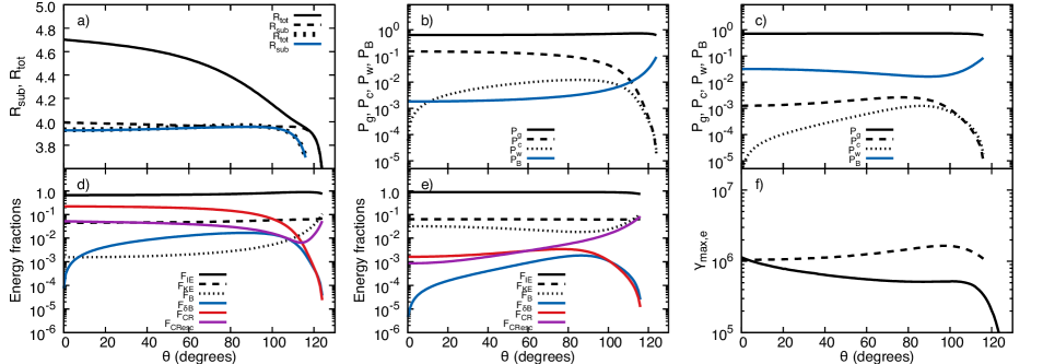
Figure 2: Selected quantities along the CD as a function of the angle $\theta$ from the secondary star. Panel a) shows the gas compression ratio across the subshock ($R_{\rm sub}$) and the entire shock ($R_{\rm tot}$). The properties for the WR-shock are shown by the black solid and dashed lines. The properties for the O-shock are shown by the black dotted and blue solid lines. Panels b) and c) show the postshock pressure (normalized to $\rho_{0}u_{0x}^{2}$) for the gas ($P_{\rm g}$), cosmic rays ($P_{\rm c}$), magnetic turbulence ($P_{\rm w}$) and uniform magnetic field ($P_{\rm B}$). Panel b) shows the properties for the WR-shock while panel c) shows the properties for the O-shock. Panels d) and e) show the downstream thermal ($F_{\rm IE}$), kinetic ($F_{\rm KE}$), magnetic ($F_{\rm B}$), magnetic turbulence ($F_{\delta\rm{B}}$) and cosmic ray ($F_{\rm CR}$) energy fractions. $F_{\rm CResc}$ is the fraction of energy in the cosmic rays that escape upstream of the shock. The total energy fraction of the cosmic rays is $F_{\rm CR}+F_{\rm CResc}$. Panel d) shows the properties for the WR-shock while panel e) shows the properties for the O-shock. Panel f) shows the maximum Lorentz factor of the non-thermal electrons from the WR-shock (solid) and the O-shock (dashed) (the maximum proton momentum is shown in Fig.1). The values in this figure are for $\Phi=\pi/4$.

Figure 3: Ratio of the turbulent to non-turbulent magnetic field as a function of angle (position) along the contact discontinuity. The properties of the WR-shock are shown by the solid line while the dotted line shows the properties of the O-shock. The post-shock magnetic field is turbulent for most of the WR-side of the CD, but is more ordered on the O-side.

3 Results

Unless otherwise noted we adopt a set of “standard” parameters for our model, in which the stellar separation is $D=2\times 10^{15}$ cm and the viewing angle $\phi=90^{\circ}$ (i.e. the line-of-sight is perpendicular to the line-of-centres between the stars - see also Fig. 1 in Pittard et al., 2020). Other parameters of our model are noted in Table 1. The model is not of any particular system, but its parameter values are chosen to be representative of a WR+O system with a reasonably wide stellar separation. For simplicity the DSA model assumes that the winds are pure hydrogen, but all other parts of the code use WC mass fractions ($X=0.0$, $Y=0.5$, $Z=0.5$) for the WR-star and solar mass fractions ($X=0.7381$, $Y=0.2485$, $Z=0.0134$; Grevesse et al., 2010) for the O-star. The wind momentum ratio is 0.1 and the stagnation point is at a distance of $0.26\,D$ from the O-star, where $D$ is the stellar separation. The WCR is largely adiabatic. Numerical values of some pre-shock quantities are given in Sec. 2.7 of Pittard et al. (2020). With a toriodal magnetic field in the wind of each star, the pre-shock magnetic flux density on the line of centres is 4 mG for the WR-shock and 20 mG for the O-shock. The shocks are almost perpendicular at this location.

3.1 The standard model

3.1.1 Quantities along each shock

Fig. 1 shows various quantites from our standard model as a function of angle, $\theta$, along the CD as measured from the secondary star ($\theta=0^{\circ}$ corresponds to the stagnation point of the WCR on the line-of-centres between the stars, while $\theta=90^{\circ}$ indicates a point on the CD where $z=D$ - see Fig. 1 in Pittard et al. (2020)). The maximum value of $\theta$ is $180^{\circ}$ minus the half-opening angle of the WCR. For our standard parameters, the half-opening angle is $\approx 50^{\circ}$, so $\theta_{\rm max}\approx 130^{\circ}$.

Fig. 1a) shows that the perpendicular pre-shock velocity is equal to $2000\,\hbox{${\rm{\rm\thinspace km}{\rm\thinspace s}^{-1}\,}$}$ on the axis of symmetry of the WCR (i.e. at the stagnation point between the winds), but steadily declines as one moves off-axis. The WR-shock becomes more oblique more rapidly than the O-shock. $u_{0x}=u_{\rm 0\perp}\rightarrow 0$ as $\theta\rightarrow\theta_{\rm max}$.

Fig. 1b) shows that the pre-shock magnetic flux density is significantly higher for the O-shock than for the WR-shock. This mainly reflects the fact that the WCR is much closer to the O-star, though there is also some enhancement due to the larger radius of the O-star. This is a key difference to our previous work (Dougherty et al., 2003; Pittard et al., 2006; Pittard & Dougherty, 2006; Pittard et al., 2020) where the on-axis pre-shock magnetic flux density was assumed to be identical for both winds.

The angle that the pre-shock magnetic field makes to the shock normal, $\theta_{\rm B0}$, is nearly $90^{\circ}$ near the stagnation point (i.e. the shock is very nearly perpendicular - see Fig. 1c). As one moves off-axis the field becomes more oblique. Note that the value of $\theta_{\rm B0}$ is a function of both $\theta$ and $\Phi$. Thus the particle acceleration is no longer azimuthally symmetric if the stars are rotating and the pre-shock magnetic field is toriodal. In such a case the shock is always perpendicular when $\Phi=0$ or $\pi$ (for all values of $\theta$). However, while it starts off perpendicular when $\Phi=\pi/2$ (when $\theta=0^{\circ}$), it becomes more and more oblique as $\theta$ increases.

Fig. 1d) shows that the pre-shock perpendicular Mach number is above 100 for both shocks up to $\theta\approx 90^{\circ}$. The pre-shock perpendicular Alfvénic Mach number is a factor of two lower than $M_{0x}$ for the WR-shock, but for the O-shock $M_{A0x}\sim 0.1M_{0x}$, so that $M_{A0x}\mathrel{\hbox to0.0pt{\lower 3.0pt\hbox{$\sim$}\hss}\raise 2.0pt\hbox{$<$}}15$ (Fig. 1e). As we will see, this drastically affects the particle acceleration efficiency of the O-shock in the standard model.

Fig. 1f) shows that the maximum non-thermal proton momentum is nearly twice as high for the O-shock. This is because the stronger magnetic field more than compensates for the reduced radius of the shock.

While the focus of Fig. 1 is mostly on pre-shock quantities along each shock, the focus of Fig. 2 is mostly on the post-shock quantities. It is immediately clear from the values of $R_{\rm tot}>4$ that the WR-shock is an efficient accelerator of non-thermal particles (until $\theta\mathrel{\hbox to0.0pt{\lower 3.0pt\hbox{$\sim$}\hss}\raise 2.0pt\hbox{$>$}}110^{\circ}$), while the O-shock is not (see Fig. 2a). The reason for this is due to the different values of $M_{\rm A0x}$ for the two shocks. When $M_{\rm A0x}$ is small enough, the compression ratios felt by the non-thermal particles ($S_{\rm sub}$ and $S_{\rm tot}$; see Eq. 3) can become significantly lower than that felt by the fluid ($R_{\rm sub}$ and $R_{\rm tot}$). This leads to a steeper spectral slope for the non-thermal particles, as noted by Bell (1978). This is discussed further in Sec. 3.1.3.

Fig. 2b) shows the various post-shock pressures, normalized to the pre-shock ram pressure, for the WR-shock. The thermal gas pressure still dominates but the cosmic ray pressure remains above 10% until $\theta>80^{\circ}$. The accelerated particles are also able to generate significant magnetic turbulence. Along a significant part of the WR-shock the turbulent field exceeds the uniform field, by up to a factor of 2. In contrast, the post-shock pressure from the non-turbulent magnetic field is the second most important pressure behind the O-shock (Fig. 2c), and the pressure from the turbulent field is lower. This means that the post-shock magnetic field is turbulent for most of the WR-side of the CD, but is more ordered on the O-side (see Fig. 3).

The WR-shock manages to convert 20% of the input energy flux into cosmic rays that are advected downstream (Fig. 2d). A further 5% goes into cosmic rays that escape upstream. In contrast, the O-shock puts $<1$% of the incoming energy flux into downstream cosmic rays (nearly 10% goes into cosmic rays that escape upstream as $\theta\rightarrow\theta_{\rm max}$, but there is very little energy going into the shock at this stage). Thus the non-thermal particles accelerated at the WR-shock will dominate the non-thermal emission, as we show in Sec. 3.1.4.

Fig. 2f) shows that radiative losses limit the maximum Lorentz factor of the non-thermal electrons to $\gamma_{\rm max,e}\sim 10^{6}$ (for the protons $\gamma_{\rm max}\mathrel{\hbox to0.0pt{\lower 3.0pt\hbox{$\sim$}\hss}\raise 2.0pt\hbox{$>$}}10^{3}$). This is slightly lower than in Pittard et al. (2020). Part of it is due to the stronger synchrotron losses that are now assumed (i.e. the use of $B_{\rm 2,tot}$ rather than $B_{0}$). The change in $\gamma_{\rm max,e}$ with $\theta$ reflects the changing pre-shock magnetic field, compression, and generation of the turbulent magnetic field.

3.1.2 The shock precursor

Fig. 4 shows pressure profiles in the WR-shock precursor as a function of position on the WCR. Panels a)-c) are for $\Phi=\pi/4$ while panels d)-f) are for $\Phi=\pi/2$ (i.e. positions on the WCR that lie in the orbital plane). Panels a)-c) show that the normalized cosmic ray pressure drops as $\theta$ increases, reflecting the drop in the acceleration efficiency. Note that there is practically no difference between panels a) and d), as the pre-shock magnetic flux density and angle to the shock normal is almost identical. However, there are significant differences between panels c) and f) since there are now much larger differences in $B_{0}$ and $\theta_{\rm B0}$ at these positions on the WR-shock.

$U_{0x}$ is almost equal to 1.0 for all of the cases in Fig. 4 (the minimum value of $U_{0x}=0.85$ is obtained for $\theta=0.5^{\circ}$). Finally, Fig. 4 shows that while the cosmic ray and turbulent magnetic pressures both increase in the precursor, there is very little increase in the thermal and magnetic pressures (again this is most obvious when $\theta=0.5^{\circ}$), indicating that there is little compression and/or heating within the precursor.

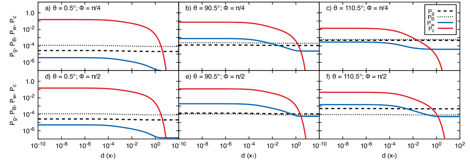
Figure 4: The normalized thermal ($P_{\rm g}$), magnetic ($P_{\rm B}$), magnetic turbulence ($P_{\rm w}$), and cosmic-ray ($P_{\rm c}$) pressures in the WR-shock precursor. The subshock is located at the left side of each panel and the upstream flow is incident from the right. The location upstream of the subshock is in units of $x_{*}=D(p_{\rm max})/u_{0x}$. Each panel shows a different location on the WR-shock front, indicated by the values of $\theta$ and $\Phi$. In all cases the normalized perpendicular pre-shock velocity $U_{\rm x}$ remains close to 1.0 (not shown).

Fig. 5 shows the profiles in the precursor of the O-shock. We see again that this shock is far less effective at accelerating particles than the WR-shock, and also that the precursor is less extended. We see that when $\Phi=\pi/4$, the normalized cosmic ray pressure immediately upstream of the subshock, $P_{\rm c1}$, is roughly constant for $\theta=0-90^{\circ}$, but drops sharply for $\theta>90^{\circ}$ (panels a-c). However, when $\Phi=\pi/2$, $P_{\rm c1}$ drops continuously with $\theta$.

Table 2 notes the values of $x_{*}$ for each position on the WCR shown in Figs. 4 and 5. Fig. 4 shows that the cosmic rays stream up to distances $\sim 10\,x_{*}$ from the WR-subshock, but are confined to distances $\ll x_{*}$ from the O-subshock. We see that the cosmic ray precursor is generally much smaller than the local scale of the shock (taken to be $r_{\rm WR}D$ and $r_{\rm OB}D$ for the on-axis ($\theta=0^{\circ}$) WR and O-shocks, respectively - for the standard model $r_{\rm WR}=0.74$ and $r_{\rm OB}=0.26$ - see also Fig. 1 in Pittard et al., 2020). While the size of the WR-shock precursor relative to the WCR starts to become significant as one moves off-axis, for the most part our use of a 1-dimensional cosmic-ray shock model is valid and appropriate. The far-off-axis region of the WCR adds little to the total cosmic-ray population and emission, in any case.

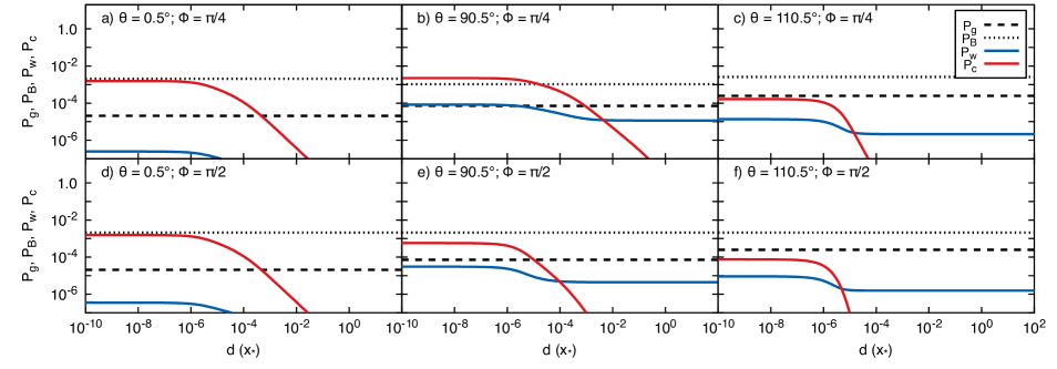
Figure 5: As Fig. 4 but for the O-shock. The precursor is less extended compared to that of the WR-shock (see Fig. 4).

Table 2: The value of $x_{*}$ in our standard model, as a function of $\theta$ and $\Phi$. The stellar separation, $D=2\times 10^{15}$ cm.

$\theta$ (∘)	$\Phi$ (c)	$x_{*}$ (cm)
		WR-shock	O-shock
0.5	$\pi/4$	$2.7\times 10^{13}$	$1.0\times 10^{13}$
0.5	$\pi/2$	$2.7\times 10^{13}$	$1.0\times 10^{13}$
90.5	$\pi/4$	$1.1\times 10^{14}$	$8.0\times 10^{13}$
90.5	$\pi/2$	$1.6\times 10^{14}$	$8.0\times 10^{13}$
110.5	$\pi/4$	$2.2\times 10^{14}$	$1.9\times 10^{14}$
110.5	$\pi/2$	$3.1\times 10^{14}$	$2.1\times 10^{14}$

3.1.3 The particle distributions

Figs. 6 and 7 show the distributions of the thermal and non-thermal particles immediately downstream of the subshock. In each figure the proton distributions are indicated by a “p”, while the electron distributions are indicated by an “e”. The particle distributions are shown for the WR-shock (solid line) and the O-shock (dashed line). Fig. 6 shows the distributions for $\theta=0^{\circ}$, while Fig. 7 shows them for $\theta=110^{\circ}$. In both cases $\Phi=\pi/4$.

The stand-out feature in both figures is the slope of the non-thermal particle distribution. The spectral index $n$ of the particle distribution ($f(p)\propto p^{n}$) is given by

$$n=-\frac{3r}{r-1},$$ (7)

where $r$ is the relevant compression ratio. For a strong, non-relativistic shock with polytropic index $\gamma=5/3$, the density compression ratio is $r=R_{\rm tot}=4$, which gives $n=-4$ (i.e. a flat distribution in our figures). However, if the scattering centres move relative to the fluid their compression ratio can be reduced, leading to steeper spectra. The on-axis WR-shock has $R_{\rm tot}=4.7$, $R_{\rm sub}=3.99$, $S_{\rm tot}=4.1$ and $S_{\rm sub}=3.5$. The spectral index of the particle distribution should therefore vary from $n=-4.2$ at low energies to $n=-3.97$ at high energies, which is indeed consistent with Fig. 6 (the high energy slope is not seen due to the maximum energy cut-off of the particles). For the on-axis O-shock we find $R_{\rm tot}=R_{\rm sub}=3.93$ but $S_{\rm tot}=S_{\rm sub}=2.45$. This yields $n=-5.1$ and is again consistent with the displayed distribution.

The stellar parameters of our standard model are not too dissimilar from those used by del Palacio et al. (2016) to model HD 93129A. It is therefore interesting that in order to match the observed synchrotron emission from HD 93129A, del Palacio et al. (2016) adopt an energy index of $p=3.2$ for the non-thermal particles in their model. This corresponds to $n=-5.2$ for the momentum index of the particles, and is very similar to the index that we find for the particles accelerated at the on-axis O-shock (see Fig. 6). del Palacio et al. (2020) also consider a hardening of the high energy particle distribution to $p=2$ (equivalent to $n=-4$), which is what we obtain for the WR-shock in our model.

In Fig. 6 the curvature of the non-thermal part of the distributions from the WR-shock reveal some modest shock modification, but it is much reduced compared to the pure hydrodynamic case (cf. Fig. 4 in Pittard et al., 2020), and this is also manifest in the shift to higher momenta of the thermal peaks. Fig. 6 again indicates that the particle acceleration at the O-shock is very inefficient. Fig. 7 shows that as $\theta$ increases the particle acceleration also becomes inefficient for the WR-shock, with the observed steepening of the particle distribution consistent with $S_{\rm sub}=2.91$ (giving $n\approx-4.6$). This behaviour again contrasts with Pittard et al. (2020) - see their Fig. 5.

Figure 6: The proton and electron distributions for the WR-shock (solid line) and O-shock (dashed line) for $\theta=0^{\circ}$ and $\Phi=\pi/4$. For the WR-shock, $R_{\rm tot}=4.7$, $R_{\rm sub}=3.99$, $S_{\rm tot}=4.1$ and $S_{\rm sub}=3.5$. For the O-shock, $R_{\rm tot}=R_{\rm sub}=3.93$ and $S_{\rm tot}=S_{\rm sub}=2.45$. For both shocks $n_{0}=1.3\times 10^{5}\,{\rm cm^{-3}}$. The thermal peaks are visible at low momenta.

Figure 7: The proton and electron distributions for the WR-shock (solid line) and O-shock (dashed line) for $\theta=110^{\circ}$ and $\Phi=\pi/4$. For the WR-shock, $R_{\rm tot}=4.02$, $R_{\rm sub}=3.96$, $S_{\rm tot}=2.96$ and $S_{\rm sub}=2.91$. For the O-shock, $R_{\rm tot}=R_{\rm sub}=3.89$ and $S_{\rm tot}=S_{\rm sub}=1.99$. For the WR-shock $n_{0}=2.0\times 10^{4}\,{\rm cm^{-3}}$, while for the O-shock $n_{0}=4.2\times 10^{3}\,{\rm cm^{-3}}$.

3.1.4 The non-thermal emission

The non-thermal emission from our standard model is shown in Fig. 8. The inverse Compton emission dominates at $E\mathrel{\hbox to0.0pt{\lower 3.0pt\hbox{$\sim$}\hss}\raise 2.0pt\hbox{$>$}}1\,$keV while synchrotron emission dominates for $E\mathrel{\hbox to0.0pt{\lower 3.0pt\hbox{$\sim$}\hss}\raise 2.0pt\hbox{$<$}}10$ eV. Free-free absorption by the stellar winds causes the synchrotron emission to turnover at about 2 GHz (which is comparable to the turnover frequency found from the full hydrodynamic models in Pittard et al., 2006). However, the Razin turnover frequency occurs at about 5 GHz and dominates the low frequency turnover in this model. The emission from $\pi^{0}$-decay adds slightly more than 10% to the total emission between $0.3-100$ GeV. The non-thermal emission in Fig. 8 is somewhat softer than that seen in Fig. 10 in Pittard et al. (2020), where a more pronounced upwards curvature in the emission towards higher energies is seen. This is due to the lower compression ratio of the scattering centres which steepens the particle distributions in the current work, and the less strongly modified shocks. The $\pi^{0}$-decay emission is also weaker relative to the inverse Compton emission in the current work, due to the lower total gas compression ratio $R_{\rm tot}$. $\gamma$-$\gamma$ absorption is negligible.

The spectral shape of the inverse Compton emission around $1-10^{3}$ eV is rather unexpected. Fig. 9 shows that this is due to emission from the particles accelerated at the O-shock, but a “bump”in the emission is also seen from particles accelerated at the WR-shock. Tests show that in both cases this “bump” is produced by electrons with Lorentz factors $\gamma<2$. It arises due to the cooling experienced by the downstream electrons, which gives rise to a “peaked” particle distribution (see Figs. 6, 7 and 10 in Pittard et al., 2020). Removing the emission from these particles creates a smooth downturn at these energies. Fig. 9 also shows that the total emission is dominated by particles accelerated at the WR-shock, and that the emission from the O-shock is noticeably softer. This is expected given the particle distributions shown in Figs. 6 and 7.

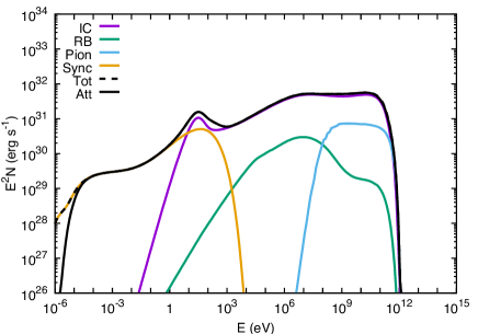
Figure 8: The non-thermal emission from our standard model. The intrinsic emission from the inverse Compton (IC), relativistic bremmstrahlung (RB), $\pi^{0}$-decay (Pion), and the synchrotron (Sync) processes are shown separately, as well as their combined total (Tot) and the total attenuated (Att) emission (which accounts for free-free and photon-photon absorption). The stellar separation $D=2\times 10^{15}\,{\rm cm}$ and the viewing angle $\phi=90^{\circ}$.

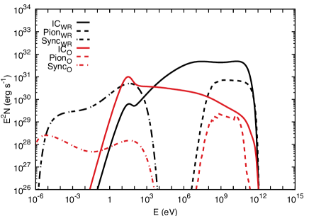
Figure 9: The contribution of each shock to the intrinsic non-thermal emission from our standard model. The emission from particles accelerated by the WR-shock is shown by the black lines, while the emission from the O-shock accelerated particles is shown by the red lines. Except for a narrow range at $\sim 10-100$ eV, the WR-shock completely dominates the non-thermal emission.

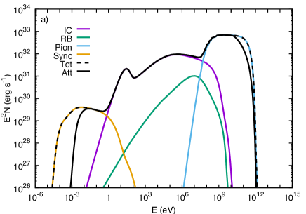
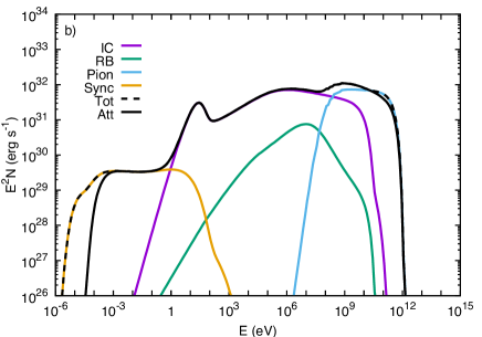
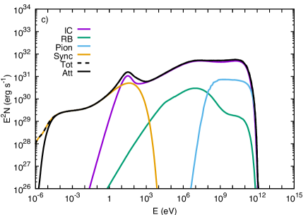
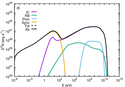
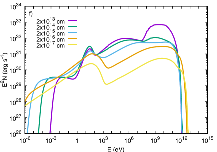
Figure 10: The dependence of the non-thermal emission on the stellar separation, $D$, which varies between each panel: a) $D=2\times 10^{13}\,{\rm cm}$; b) $D=2\times 10^{14}\,{\rm cm}$; c) $D=2\times 10^{15}\,{\rm cm}$; d) $D=2\times 10^{16}\,{\rm cm}$; e) $D=2\times 10^{17}\,{\rm cm}$. All other parameters are unchanged. In panel f) the total attenuated emission from each of these models is plotted. In all cases $\phi=90^{\circ}$.

3.2 The effect of varying the stellar separation

Fig. 10 shows how the non-thermal emission changes as the stellar separation is varied. It is clear that the $\pi^{0}$-decay emission increases steadily as $D$ decreases (scaling as $D^{-1}$ - see Pittard et al., 2020). So while the non-thermal spectrum at large $D$ is dominated by synchrotron and inverse Compton emission (at low and high energies, respectively), at closer separations the high energy emission becomes dominated by the $\gamma$-rays created by $\pi^{0}$-decay (emission from secondary electrons may also become important - see Sec. 3.4). At $D=2\times 10^{17}$ cm the synchrotron emission dominates up to $E=1$ keV, while at higher energies inverse Compton emission takes over. As $D$ decreases the spectral shape of the synchrotron emission changes quite markedly, due to a softening of the non-thermal electron spectrum. The maximum energy of the inverse Compton emission is $\mathrel{\hbox to0.0pt{\lower 3.0pt\hbox{$\sim$}\hss}\raise 2.0pt\hbox{$>$}}10^{12}$ eV at $D\mathrel{\hbox to0.0pt{\lower 3.0pt\hbox{$\sim$}\hss}\raise 2.0pt\hbox{$>$}}10^{15}$ cm, but decreases for closer separations, being $\sim 10^{10}$ eV when $D\sim 10^{13}$ cm. $\gamma$-$\gamma$ absorption only becomes significant at $D\mathrel{\hbox to0.0pt{\lower 3.0pt\hbox{$\sim$}\hss}\raise 2.0pt\hbox{$<$}}10^{14}$ cm.

Pittard et al. (2020) showed that the emission from non-thermal electrons varies in a more complicated way with $D$. If the cooling length of the non-thermal electrons is greater than or of order the size of the WCR, then they fill the WCR and the emission also varies as $D^{-1}$. However, if the non-thermal electrons cool more rapidly then the emission will tend towards a constant value (i.e. be independent of $D$). They also noted that as $p_{\rm max,e}\propto D^{-1}$ (for an assumed scaling of $B_{0}\propto D^{-1}$), this would drive further changes in the emission with $D$.

Panel f) in Fig. 10 shows the total attenuated non-thermal spectrum at each distance. For $E\mathrel{\hbox to0.0pt{\lower 3.0pt\hbox{$\sim$}\hss}\raise 2.0pt\hbox{$>$}}10^{3}$ eV the emission generally increases with decreasing $D$, though depending upon the energy, the increase is not always steady or even strictly monotonic. As $D$ drops further the emission plateaus, as predicted by Pittard et al. (2020). Free-free absorption by the clumpy stellar winds curtails the low-frequency synchrotron emission as $D$ decreases, with the turnover frequency scaling as $\nu\propto D^{-10/7}$ (Dougherty et al., 2003). The Razin effect produces a characteristic cut-off frequency that is given by $\nu_{\rm R}=20n_{\rm e}/B$. Since in our standard model $B\propto 1/D$ and $n_{\rm e}\propto 1/D^{2}$, the cut-off frequency scales as $\nu_{\rm R}\propto D^{-1}$. This is responsible for the turndown in the intrinsic synchrotron emission seen in Fig. 10.

3.3 The effect of varying the stellar wind magnetic field

The pre-shock magnetic field depends on the strength of the magnetic field at the stellar surfaces, $B_{*}$, and the rotation speed of the star, $v_{\rm rot}$. The latter affects how tightly wound the field-lines are in the equatorial plane of the star. In the extreme case that the stars are not rotating the stellar wind drags the field lines into a radial configuration. In the following we vary both $B_{*}$ (specifically the surface magnetic field of the O-star, $B_{\rm*O}$) and $v_{\rm rot}$ to see how each may change the particle acceleration and non-thermal emission.

3.3.1 Changing the surface magnetic field

We first explore changing $B_{*}$. Since $B_{0}$ is higher for the O-shock than it is for the WR-shock in the standard model (see Fig. 1), we reduce the surface magnetic field strength of the O-star to $B_{\rm*O}=10$ G (the standard model has $B_{*}=100$ G for both stars). This results in an on-axis pre-shock magnetic field strength of 2.1 mG and an Alfvénic Mach number of 155 at the O-shock. The result is that the on-axis O-shock becomes much more efficient at accelerating particles than before, with 45% of the incoming kinetic flux now turned into non-thermal particles flowing downstream from the shock. This is a greater efficiency than the on-axis WR-shock (which is at 23%), and is also manifest as a higher compression ratio for the O-shock ($R_{\rm tot}=7.2$) in this situation.

We find that the particle acceleration process behaves non-linearly with the magnetic field strength at the shock. As the surface magnetic field of the O-star reduces from $100$ G the particle acceleration efficiency at the O-shock first increases and then reduces again. This is because of two competing effects. First, the acceleration efficiency increases as the Alfvénic Mach number of the shock increases. Second, the maximum proton energy decreases ($E_{\rm max}\propto B_{0}$ - see Sec. 2.2.2) - this eventually causes the acceleration to become inefficient.

This non-linear behaviour is manifest in the resulting non-thermal emission which is shown in Fig. 11. The dependence of the particle acceleration efficiency on $M_{\rm A0x}$ and $p_{\rm max}$ results in the peak of the synchrotron emission being obtained at an intermediate value of $B_{\rm*O}$.

Considering the IC emission in Fig. 11b), we see that the IC emission has a globally negative slope when $B_{\rm*O}=100$ G, while the curves for lower values of $B_{\rm*O}$ do not. This arises because of the very steep particle distributions that are obtained when $B_{\rm*O}=100$ G (the standard case) due to the low values of $S_{\rm tot}$ and $S_{\rm sub}$ (see Fig. 6). As $B_{\rm*O}$ decreases and $S_{\rm tot}$ and $S_{\rm sub}$ increase, the IC emission attains a globally positive slope.

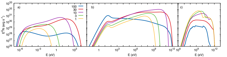
Figure 11: The intrinsic non-thermal emission from the particles accelerated at the O-shock when the surface magnetic field of the O-star is varied. a) The synchrotron emission. b) The inverse Compton emission. c) The emission from $\pi^{0}$-decay.

3.3.2 Radial stellar magnetic fields

We now explore how the particle acceleration and emission changes if we assume that the stars do not rotate. This results in a radial magnetic field in each stellar wind, which declines as $r^{-2}$ (instead of a toroidal field that declines as $r^{-1}$). Hence this change affects both the strength of the pre-shock magnetic field, and its orientation to the shock. On the WCR axis the shocks become parallel (compared to almost perpendicular in the standard model).

Fig. 12 shows the pre-shock quantities as a function of the angle $\theta$ from the secondary star for the WR and O winds. Because the magnetic field in each stellar wind is now radial, and drops as $r^{-2}$, the pre-shock magnetic flux density is considerably lower than in the standard model, especially for the WR-shock. This results in both shocks becoming highly super-Alfvénic ($M_{\rm A0x}>10^{4}$ for the WR-shock, and $M_{\rm A0x}\sim 10^{3}$ for the O-shock). Both shocks are parallel on-axis and become nearly perpendicular far off-axis. The reduced magnetic field strength also lowers the maximum momentum that the non-thermal protons attain (again, particularly for the WR-shock).

Figure 12: As Fig. 1 but for a model where the stars are not rotating, resulting in a radial magnetic field in each wind. All quantities are now independent of $\Phi$.

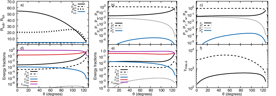
Figure 13: As Fig. 2 but for a model where the stars are not rotating, resulting in a radial magnetic field in each wind. All quantities are now independent of $\Phi$.

Fig. 13 shows the post-shock quantities as a function of the angle $\theta$ from the secondary star. Both the WR-shock and O-shock are now extremely efficient particle accelerators, and very high compression ratios are obtained. The latter occurs despite creation of non-negligible magnetic turbulence at the shock because of the very low magnetic field strength upstream. On axis the WR-shock puts 12 and 87 per cent of the incoming kinetic flux into non-thermal particles that flow downstream and escape upstream, respectively. For the O-shock these numbers are 32 and 65 per cent. The thermal X-ray emission from the WCR (not calculated) will be much softer from this model than the terminal speeds of the winds would suggest, because of the significantly lower post-shock temperatures that are obtained (as a large part of the input mechanical energy is used for particle acceleration). The turbulent magnetic field component dominates the uniform field component, for both shocks and in all locations, by more than an order of magnitude.

Another big change is the dramatic reduction in the maximum Lorentz factor of the non-thermal electrons. We see that $\gamma_{\rm max,e}$ drops from $\sim 10^{6}$ with a toroidal stellar magnetic field (see Fig. 2f) to $\sim 10^{3}$ when the field is radial. This is due to several factors: i) the large reduction in the flow speed immediately prior to the subshock (due to the large compression in the subshock in this model, $u_{1}=u_{0}R_{\rm sub}/R_{\rm tot}=92\hbox{${\rm{\rm\thinspace km}{\rm\thinspace s}^{-1}\,}$}$, compared to $1700\hbox{${\rm{\rm\thinspace km}{\rm\thinspace s}^{-1}\,}$}$ in the standard model); ii) the low value of the magnetic field immediately prior to the subshock ($B_{1}=2.6\times 10^{-5}$ G in this model, compared to $5\times 10^{-3}$ G in the standard model); iii) the strongly turbulent post-shock magnetic field ($B_{\rm 2,tot}=0.044$ in this model, versus 0.02 in the standard model). Factors i) and ii) strongly reduce the acceleration rate of the electrons (cf. Eq. 5), by about a factor of $10^{5}$, while iii) increases the synchrotron loss rate by a factor of $\approx 5$.

Fig. 14 shows the on-axis particle distributions immediately downstream of the subshock. The strong concave curvature to the distributions indicates the significant modification of the shocks. The O-shock now contributes similarly to the non-thermal particle population, whereas in the standard model the O-shock contributed very little (cf. Fig. 6). Neither shock accelerates particles to particularly high energies, and as we have seen the electron maximum energy is considerably reduced. The thermal peak shows a significant shift to lower momenta, particularly for the WR-shock, indicating the considerable reduction in post-shock temperature.

Figure 14: The proton and electron distributions for the WR-shock (solid line) and O-shock (dashed line) for $\theta=0^{\circ}$ when the magnetic field in each stellar wind is radial. The distributions are independent of $\Phi$. For the WR-shock, $R_{\rm tot}=S_{\rm tot}=54.1$ and $R_{\rm sub}=S_{\rm sub}=2.5$. For the O-shock, $R_{\rm tot}=19.8$ and $R_{\rm sub}=3.09$, while $S_{\rm tot}=19.6$ and $S_{\rm sub}=3.06$. For both shocks $n_{0}=1.3\times 10^{5}\,{\rm cm^{-3}}$. The thermal peaks are visible at low momenta. $D=2\times 10^{15}$ cm.

In Fig. 15 we show the non-thermal emission from this model. The differences in the non-thermal particle distributions compared to the standard model result in significant differences to the non-thermal emission. First, we see a dramatic dip in the emission between energies of $0.1-10$ eV. This is caused by the significantly lower energies attained by the non-thermal electrons, which causes a reduction in the number of energy decades that the synchrotron (and inverse Compton) emission extends over. Second, the synchrotron and inverse Compton emission are both significantly weaker. Third, the reduction in $p_{\rm max}$ also lowers the maximum energy of the $\pi^{0}$-decay emission. Finally, we see that the $\pi^{0}$-decay emission is significantly stronger compared to the standard model at the same separation. This is because of the much higher density of the post-shock gas due to the increased compression of the shocks, plus the much lower flow speed of this gas, which means that the ratio of the non-thermal proton cooling timescale to the flow timescale has much reduced.

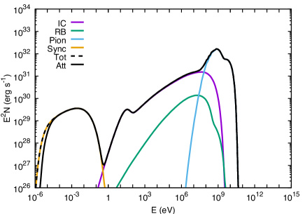
Figure 15: The non-thermal emission when the stellar rotation speeds are zero (in the standard model $v_{\rm rot}/\hbox{${v_{\infty}}$}\,=0.1$). $D=2\times 10^{15}$ cm.

3.4 Secondary electron creation and emission

In some situations we might expect secondary electrons to make an important contribution to the overall emission. Secondary electrons can be created when non-thermal protons interact with either thermal protons or with photons. The former case is expected to be dominant in CWBs (see App. D). The emission from secondary electrons has the potential to dominate that from the primary electrons (those accelerated at the shocks) because the former originate from the non-thermal protons, which carry the majority of the energy that the non-thermal particles have (see, e.g., Orellana et al., 2007). It is also possible to create secondary electrons with higher maximum energies than the primary electrons (since the former is given by $0.05\,E_{\rm p,max}$, where $E_{\rm p,max}$ is the maximum proton energy, while the latter depends on inverse Compton and synchrotron losses during shock acceleration). The secondary electrons have the same slope in their particle distribution as the primary protons.

In order for secondary electrons to dominate the emission the non-thermal protons must lose a significant fraction of their energy through collisions with thermal protons. The inelastic proton-proton cross-section is energy dependent, but we can take $\sigma_{\rm pp}\approx 30\,$mb as a good approximation (see, e.g., Fig. A2 in Vila, 2012, and also Eq. 32 in this work). The cooling rate of a non-thermal proton is then

$$\frac{1}{t_{\rm pp}}\approx cn_{\rm p}K_{\rm pp}\sigma_{\rm pp},$$ (8)

where $n_{\rm p}$ is the thermal proton number density and $K_{\rm pp}\approx 0.5$ is the total inelasticity of the interaction.

For cooling to be effective we require $t_{\rm pp}\mathrel{\hbox to0.0pt{\lower 3.0pt\hbox{$\sim$}\hss}\raise 2.0pt\hbox{$<$}}t_{\rm dyn}=D/v_{\rm ps}$, where $v_{\rm ps}$ is the postshock flow speed. With $v_{\rm ps}\sim v_{\infty}/R_{\rm tot}$ and $n_{\rm p}\sim R_{\rm tot}\hbox{${\dot{M}}$}/(4\pi D^{2}v_{\infty}m_{\rm H})$, this gives

$$D\mathrel{\hbox to0.0pt{\lower 3.0pt\hbox{$\sim$}\hss}\raise 2.0pt\hbox{$<$}}10^{12}\frac{\hbox{${\dot{M}}$}_{-5}R_{\rm tot}^{2}}{v_{\infty,3}}\,{\rm cm},$$ (9)

where $\hbox{${\dot{M}}$}_{-5}=\hbox{${\dot{M}}$}/(10^{-5}\hbox{${\rm\hbox{${\rm\thinspace M_{\odot}}$}{\rm\thinspace yr}^{-1}\,}$})$ and $v_{\infty,3}=v_{\infty}/(1000\hbox{${\rm{\rm\thinspace km}{\rm\thinspace s}^{-1}\,}$})$. For our standard model $\hbox{${\dot{M}}$}_{-5}=2$ and $v_{\infty,3}=2$ for the primary star, and $R_{\rm tot}\sim 4$, so secondary electrons should become important when $D_{\rm sep}\mathrel{\hbox to0.0pt{\lower 3.0pt\hbox{$\sim$}\hss}\raise 2.0pt\hbox{$<$}}2\times 10^{13}\,{\rm cm}$.

Fig. 16 compares the leptonic and total non-thermal emission arising from models that include or do not include secondary electrons. We see that the secondary electrons give a significant boost to the high energy inverse Compton emission (over the energy range $E=10^{5}-10^{11}$ eV) and synchrotron emission (over the energy range $E=10^{-3}-10^{4}$ eV), and indeed emit at higher energies than the primary electrons are capable of. The emission produced by secondary electrons is aided by the fact that they are continually generated downstream (whereas the primary electrons cool as they flow downstream and so only have a short opportunity to create the highest energy synchrotron and inverse Compton emission).

Despite the significant boost to the leptonic emission that the secondaries provide, however, there is relatively little change in the spectrum of the total non-thermal emission. The reason is that at the energies where this boost to the emission occurs, other processes tend to be dominant (inverse Compton emission from the primary electrons masks the synchrotron emission from secondary electrons at $E\sim 10-10^{3}$ eV, and $\pi^{0}$-decay emission at $E\sim 10^{8}-10^{11}$ eV masks the inverse Compton emission from secondary electrons). Only between $10^{5}-10^{8}$ eV do the secondary electrons make a visible contribution to the total emission.

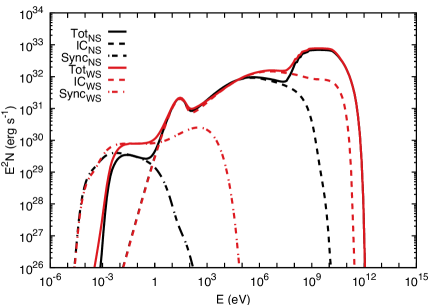
Figure 16: Comparison of the intrinsic non-thermal emission from models with (subscript WS; red lines) and without (subscript NS; black lines) secondary electrons ($D=2\times 10^{13}$ cm). The secondary electrons boost the inverse Compton and synchrotron emission.

While secondary electrons do not appear to significantly affect the total non-thermal emission for the standard model parameters with $D\mathrel{\hbox to0.0pt{\lower 3.0pt\hbox{$\sim$}\hss}\raise 2.0pt\hbox{$>$}}10^{13}$ cm, they may be more important in systems with higher stellar mass-loss rates and slower wind speeds, or if the primary protons are able to interact with dense, radiatively cooled, gas. White et al. (2020) show that secondary electrons dominate the emission between $E\approx 1-40$ MeV in their “off-periastron” models of $\eta$ Carinae (see the top panel in their Fig. 3).

Secondary electrons can also become important in situations where the shocks are strongly modified and very high compression ratios are achieved. Fig. 17 compares the significance of secondary electrons in such models (see Fig. 13 for the $R_{\rm tot}$ values in this case). While secondary electrons only become important for stellar separations $D\mathrel{\hbox to0.0pt{\lower 3.0pt\hbox{$\sim$}\hss}\raise 2.0pt\hbox{$<$}}2\times 10^{13}\,$cm in models with the standard parameters, Fig. 17 shows that secondaries can become important at much wider stellar separations when the shocks are significantly modified. In this particular case they are starting to add significantly to the emission between $10^{5}-10^{7}$ eV.

Figure 17: Comparison of the non-thermal emission from models with and without secondary electrons. $D=2\times 10^{15}$ cm and $v_{\rm rot}/\hbox{${v_{\infty}}$}\,=0.0$ (i.e. the stellar winds have radial magnetic fields).

4 Modelling the radio emission from WR 146

Having explored how the particle acceleration and non-thermal emission varies with stellar separation and the magnetic field in each wind, and the conditions under which secondary electrons become important, we now turn our attention to the modelling of a specific system. We choose WR 146, a WC6+O8I-IIf system (Lépine et al., 2001), because it is amongst the brightest CWBs at radio wavelengths and is also one of the few CWBs to be spatially resolved, with a southern thermal component and a northern non-thermal component (Dougherty et al., 1996, 2000; O’Connor et al., 2005). It has also been resolved at optical wavelengths by HST (Niemela et al., 1998), revealing a projected stellar separation of $168\pm 31$ mas with the WR-star to the south and the O-star to the north. At 43 GHz there is a significant thermal contribution to the northern flux from the O-star wind (O’Connor et al., 2005). From the relative position of the components, O’Connor et al. (2005) inferred a wind momentum ratio of $\eta=0.06\pm 0.15$. More recently, a search for polarized radio emission has been made (Hales et al., 2017). WR 146 is currently the only CWB system to be detected at frequencies as low as 150 MHz (Benaglia et al., 2020). The distance to WR 146 is estimated as $1.2\pm 0.3$ kpc (Dougherty et al., 1996), which is compatible with the Gaia DR2 estimate of $1.10^{+0.67}_{-0.36}$ kpc (Rate & Crowther, 2020). At a distance of $1.2$ kpc, the projected stellar separation is $2.9\times 10^{15}$ cm. Secondary electrons are not expected to be important in this system (see Eq. 9), and are therefore not included in the following models.

In their X-ray analysis of WR 146, Zhekov (2017) found that the predicted theoretical X-ray flux from their models far exceeded the observed emission. To bring the two measurements together required either substantially reducing their adopted mass-loss rates (by a factor of 10), or increasing the stellar separation $D$ (by a factor of 66). The necessary change required for each variable in isolation is rather implausible, which suggests that they need to vary in combination, though even then the size of the required changes is rather overwhelming. One then wonders what other process could be at play. Zhekov (2017) note that models where the post-shock electrons are not in temperature equilibration with the ions can reduce the X-ray luminosity by another factor of two.

There seem to be three possible solutions to this problem. First, the wind momentum ratio may be too high (Zhekov (2017) assumed that $\eta=0.11$). A lower value would mean that a smaller fraction of the WR wind is shocked, and since $L_{\rm x}\propto\eta$ (Pittard & Dawson, 2018), this would move the theoretical prediction towards the observed flux. However, given the magnitude of the excess emission this alone will not be enough. A second solution, which is not incompatible with the previous one, is that a significant fraction of the kinetic power of the stellar winds goes into non-thermal particles via DSA. Both of these possibilities are investigated below. Finally, a third possibility is that the post-shock flow is also not in ionization equilibrium. This may impact the X-ray luminosity but a detailed study is needed to determine at what level.

Our spectral models of WR 146 are constrained by the observed flux from this system. In the radio band we use the flux measurements by Hales et al. (2017) and Benaglia et al. (2020). We also include measurements obtained using the VLA in combination with the VLBA Pie Town antenna (see Table 3). In the X-ray band we use the on-axis ACIS-I Chandra pointed observation (Obs ID 7426) taken on March $17^{\rm th}$ 2007 (PI Pittard). This observation was designed to search for signs of weak shock heating and shock modification. Finally, there are also upper limits from 2 years of data from the Fermi satellite (Werner et al., 2013). To date, only one CWB has been detected at TeV energies ($\eta$ Carinae; H.E.S.S. collaboration, 2020).

Table 3: Flux and RMS measurements of WR 146 obtained with the VLA in combination with the VLBA Pie Town antenna on October 1^st 2004 (the 22 GHz data was obtained on November 8^th 2004). Where two sources are resolved data is provided for both. At the lower frequencies where this is not the case all the flux is assigned to the northern source. From O’Connor et al. (2005).

Frequency	N flux	N RMS	S flux	S RMS
(GHz)	(mJy)	(mJy)	(mJy)	(mJy)
1.465	71.92	1.4	0.0	0.0
4.885	33.96	0.68	0.0	0.0
8.435	23.46	0.47	0.0	0.0
15.00	14.82	0.74	3.59	0.18
22.46	10.33	0.52	5.17	0.26
43.34	5.21	0.26	6.59	0.33

Table 4: The parameters used in our final model of WR 146. Our assumed $D=1.2\times 10^{16}$ cm implies that $i=76^{\circ}$ and $\phi=14^{\circ}$ (the O star is directly in front of the WR-star when $i=90^{\circ}$). The WR-star terminal wind speed is an average from Eenens & Williams (1994) and Willis et al. (1997). The O-star terminal wind speed is from the velocity ratio given in Dougherty et al. (2000). The O and WR-star luminosities are from O’Connor (private communication), and are estimated from Vacca, Garmany & Shull (1996) and the magnitude difference reported by Niemela et al. (1998). The hydrogen, helium and “metal” mass fractions are noted as $X$, $Y$ and $Z$, respectively. The WR abundances are from Nugis & Lamers (2000).

Parameter	WR-star	O-star
$\hbox{${\dot{M}}$}\,\,(\hbox{${\rm\hbox{${\rm\thinspace M_{\odot}}$}{\rm\thinspace yr}^{-1}\,}$})$	$2\times 10^{-5}$	$4\times 10^{-6}$
$v_{\rm\infty}\,\,(\hbox{${\rm{\rm\thinspace km}{\rm\thinspace s}^{-1}\,}$})$	$2800$	$1600$
$L\,\,(\hbox{${\rm\thinspace L_{\odot}}$})$	$2.3\times 10^{5}$	$7.9\times 10^{5}$
$T_{\rm eff}\,\,$(K)	49000	32000
$R_{*}\,\,(\hbox{${\rm\thinspace R_{\odot}}$})$	6.6	28.9
$X$	0.0	0.7381
$Y$	0.744	0.2485
$Z$	0.256	0.0134
$B_{*}$  (G)	140	14
$v_{\rm rot}/\hbox{${v_{\infty}}$}\,$	0.1	0.1
$f$	1.0	1.0

Table 5: The kinetic power of the winds, the kinetic flux at each shock, and the power put into non-thermal particles that are advected downstream or escape upstream from the shocks. All values are in ${\rm{\rm\thinspace erg}{\rm\thinspace s}^{-1}\,}$.

Parameter	WR	O	Total
Wind kinetic power	$5.0\times 10^{37}$	$3.3\times 10^{36}$	$5.3\times 10^{37}$
Input power at shock	$1.6\times 10^{36}$	$8.9\times 10^{35}$	$2.5\times 10^{36}$
CR advection power	$3.4\times 10^{35}$	$2.4\times 10^{35}$	$5.7\times 10^{35}$
CR escape power	$6.7\times 10^{34}$	$6.9\times 10^{34}$	$1.4\times 10^{35}$

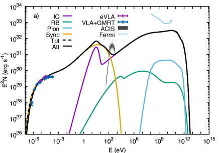
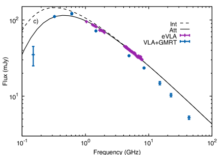
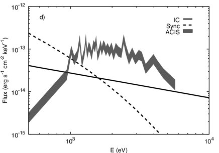
Figure 18: Model spectra for WR 146. a) The model inverse Compton, synchrotron, relativistic bremsstrahlung and $\pi^{0}$-decay emission are shown, together with the observed radio and thermal X-ray fluxes, and the upper limits from Fermi. b) The inverse Compton and synchrotron emission from particles accelerated at the WR-shock (black lines) and O-shock (red lines). c) The intrinsic and absorbed synchrotron radio emission from the model, and the observed radio emission. d) The observed X-ray emission and the non-thermal emission from the model. See Table 4 for the model parameters.

4.1 The modelling

As it is unlikely that the stars are not rotating we adopt $v_{\rm rot}/v_{\infty}=0.1$, which leads to a toroidal magnetic field in each wind. We first attempted to fit the observational data with the assumption that the system is viewed face-on ($D=2.9\times 10^{15}$ cm; $i=0^{\circ}$; $\phi=90^{\circ}$). We adopted somewhat lower mass-loss rates than usually found in the literature, given the findings by Zhekov (2017): $\hbox{${\dot{M}}$}_{\rm WR}=2\times 10^{-5}\,\hbox{${\rm\hbox{${\rm\thinspace M_{\odot}}$}{\rm\thinspace yr}^{-1}\,}$}$ and $\hbox{${\dot{M}}$}_{\rm O}=2\times 10^{-6}\,\hbox{${\rm\hbox{${\rm\thinspace M_{\odot}}$}{\rm\thinspace yr}^{-1}\,}$}$. With the observed terminal wind speeds this gives a wind momentum ratio $\eta=0.057$. However, it proved impossible to obtain a good match to the observed synchrotron emission while simultaneously matching the turnover frequency at $\nu\approx 450\,$MHz. In particular we found that the Razin turnover frequency was always too high, and the synchrotron luminosity too low. The former could be reduced by reducing the stellar surface magnetic flux densities, but this led to lower synchrotron luminosity (cf. Fig. 11).

Since $\nu_{\rm R}\approx 20\,n_{\rm e}/B\,$, the Razin turnover frequency can be lowered in the case that $B\propto 1/D$ by increasing $D$. Increasing the stellar separation to $D=1.2\times 10^{16}$ cm ($i=76^{\circ}$; $\phi=14^{\circ}$) yielded $\nu_{\rm R}$ at the correct frequency, but the synchrotron luminosity was still too low. To increase the synchrotron luminosity the O-star mass-loss rate was increased to $\hbox{${\dot{M}}$}_{\rm O}=4\times 10^{-6}\,\hbox{${\rm\hbox{${\rm\thinspace M_{\odot}}$}{\rm\thinspace yr}^{-1}\,}$}$, giving a wind momentum ratio $\eta=0.11$. This increase in $\eta$ means that a greater fraction of the WR-wind kinetic flux is intercepted by the WCR. The kinetic flux of the O-wind also doubles. The increase in $\hbox{${\dot{M}}$}_{\rm O}$ and $\eta$ does indeed produce stronger synchrotron emission, and a reasonable match to the observational data is now obtained (see Fig. 18). With the assumed value of $v_{\rm rot}/\hbox{${v_{\infty}}$}\,=0.1$ we require $B_{\rm*WR}\approx 140$ G and $B_{\rm*O}\approx 14$ G to match the turnover frequency and synchrotron flux. The turndown below 1 GHz is a combination of the Razin effect and free-free absorption (see Fig. 18c). The latter is sensitive to the volume filling factor of the clumps in the winds - here the winds are assumed to be smooth (i.e. $f=1.0$; since the thermal free-free emission from the stellar winds is not calculated in our model, $f$ only affects the free-free absorption through the O-wind in the current model). While our model is a good match to the recent eVLA data of Hales et al. (2017) and the GMRT data of Benaglia et al. (2020), it matches less well the derived fluxes from the older VLA + Pie Town data of O’Connor et al. (2005), which lie below the higher fluxes reported by Hales et al. (2017). The parameters of our model are noted in Table 4.

In our model the non-thermal particles accelerated at the WR-shock provide the majority of the emission, with the O-shock accelerated particles typically contributing about a third to the total flux. The WR-shock accelerated particles provide the highest energy inverse Compton and synchrotron emission (see Fig. 18b). The non-thermal X-ray flux predicted by the model is shown together with the observed X-ray emission in Fig. 18d). The inverse Compton emission barely drops below the observed thermal emission at $E\approx 6$ keV, while the predicted synchrotron emission exceeds the observed thermal emission at $E<1$ keV (note that no photoelectric absorption has been applied to the model emission). In our model the synchrotron flux at keV energies is sensitive to the value adopted for $\alpha$ in Eq. 4 and the assumption that the synchrotron loss rate at the shock depends on $B_{\rm 2,tot}$ (this latter assumption affects $p_{\rm max,e}$). Both of these “close encounters” with the thermal X-ray emission may prove challenging to future models. In theory, they may allow tight constraints to be placed on the O-star luminosity (a higher luminosity would possibly decrease the maximum energy of the non-thermal electrons and thus the maximum energy that the synchrotron emission attains, but then would increase the predicted inverse Compton emission, while a lower luminosity would increase the maximum energy of the synchrotron emission). Future models should also investigate whether radial magnetic fields in the stellar winds produce a better match to the observations.

On axis the shocks put $\approx 20$ per cent of the wind kinetic flux into non-thermal particles, while a further 5 per cent goes into non-thermal particles that escape upstream. Compression ratios of 4.7 are obtained. The upstream magnetic field strength is 0.72 and 0.93 mG for the WR and O-shock respectively, while the post-shock values are 3.4 and 4.3 mG.

Table 5 notes the kinetic power of each wind, the power available at each shock, and the power put into non-thermal particles that are advected downstream or escape upstream of each shock. The total power put into non-thermal particles is $7.1\times 10^{35}\,\hbox{${\rm{\rm\thinspace erg}{\rm\thinspace s}^{-1}\,}$}$, which represents an overall efficiency of conversion of the power available at the shocks of 29 per cent. Just over 1 per cent of the combined wind power of the stars goes into non-thermal particles.

4.2 Discussion

Compared to the model in Zhekov (2017), $\hbox{${\dot{M}}$}_{\rm WR}$ is 1.6 times lower, $D$ is 3.5 times higher, and $\eta$ is the same. Since the thermal X-ray luminosity for an adiabatic system scales as $L_{\rm x}\propto\hbox{${\dot{M}}$}^{2}\eta D^{-1}$ (Stevens et al., 1992; Pittard & Dawson, 2018), our model should be 9 times fainter by this measure. However, as 30 per cent of the available wind power is put into cosmic rays rather than thermalised gas, it should be $\approx 13$ times fainter overall. Unfortunately, this is still less than the factor of $30-50$ reduction that Zhekov (2017) states is required if $T_{\rm e}\leq T_{\rm ion}$. Perhaps non-equilibrium ionization also has a role to play.

Turning our attention to the radio we note that although synchrotron emission is intrinsically polarized, Hales et al. (2017) found the fractional linear polarization from the radio synchrotron emission from WR 146 to be less than 0.6 per cent. The lack of polarization is naturally explained if the magnetic field is turbulent, and they estimate that the field has a dominant random component with $\delta B/B>8$. In contrast, we find that the emission weighted value of $\delta B/B$ from our model is $\approx 2.4$ at frequencies of $1-8$ GHz. This suggests that some other process or mechanism may be responsible for the lack of polarisation (see Hales et al. (2017) for a discussion of this). Alternatively, it may indicate that our models of WR 146 should have a magnetic field that is more turbulent. This is achieved in our model with radial magnetic fields in the stellar winds (see Sec. 3.3.2), where the turbulent component dominates for both shocks in all locations by more than an order of magnitude. The level of turbulence is interesting not least because a high level of turbulence may lead to ultra-fast acceleration in CWBs (and maximum energies above a few TeV), in contrast to SNRs which appear to accelerate particles close to the Bohm limit (Stage et al., 2006).

While we have indicated the simple fitting that we have attempted, we have certainly not exhausted all possibilities, and it is quite likely that fits as least as good will be found with other model parameters. This is because various trade-offs exist between the model parameters. For instance, increasing $D$ generally leads to a drop in emission, but this can be offset by increasing ${\dot{M}}$. In addition, $B_{*}$ and $v_{\rm rot}/\hbox{${v_{\infty}}$}\,$ can be directly played off against each other. Having said this, the model does place some constraints. Too high values for the magnetic flux density result in particle distributions that are too steep. Too low values for $B$ result in no or very weak acceleration, and/or too low values of $p_{\rm max}$ and $p_{\rm max,e}$. A more detailed investigation, that will also model the free-free radio emission, the thermal X-ray emission, and produce radio images, is left to future work.

5 Summary and conclusions

We report on the first particle acceleration model of colliding wind binaries that applies a non-linear diffusive shock acceleration model, with magnetic field amplification and relative motion of the scattering centres, to oblique shocks. We find that:

1. The relative motion of the scattering centres with respect to the fluid can be significant. When this occurs we obtain steeper non-thermal particle distributions.

2. The particle acceleration is strongly dependent on the pre-shock magnetic field, and its efficiency can vary strongly along and between each shock.

3. The particle acceleration efficiency and non-thermal emission can behave non-linearly with the magnetic field strength at the shock. As the pre-shock magnetic flux density decreases, an increase in acceleration efficiency due to the increasing Alfvénic Mach number competes against a reduction in the maximum energy of the accelerated particles. This can result in the non-thermal emission peaking at intermediate values of the magnetic field strength.

4. The strength and angle to the shock normal of the pre-shock magnetic field depends strongly on whether the stellar winds have a toroidal field (i.e. the stars are rotating) or a radial field (i.e. the stars are non-rotating).

5. The non-thermal emission may be dominated by particles accelerated by one or the other shock, or may be roughly equally split between both shocks.

6. The shock precursors are typically smaller than the scale of the WCR.

7. Downstream of the shock the dominant pressure may be from the gas or from the cosmic rays.

8. In some locations along the shocks we find that $\delta B>B$, while the opposite is true in other locations. In our standard model we find that the WR-shock is largely turbulent while the O-shock is not. Whether or not a shock is turbulent depends sensitively on the model parameters, such as the strength of the surface magnetic field and rotation speed of the star. In some systems the synchrotron emission should not be significantly polarized, while in others it may be.

9. Local particle acceleration efficiencies for the downstream flowing cosmic rays of up to 30 per cent are obtained. Such values can arise when the shocks are perpendicular, oblique, or parallel. When the magnetic field in the stellar wind is radial, the lower pre-shock magnetic flux densities that result mean that up to nearly 90 per cent of the local kinetic flux may go into cosmic rays that escape upstream. Under other conditions the advected and escape cosmic ray energy fractions may be much reduced.

10. The gas compression ranges from $\leq 4$ to over 20 in some cases. High ratios have a significant effect on the strength of the emission from $\pi^{0}$-decay and secondary electrons, and will also affect the postshock temperature and the thermal X-ray emission.

Given the large variation in the spectral indices of the non-thermal particles seen in our models, it is clearly necessary to go beyond the assumption that $f(p)\propto p^{-4}$ (equivalent to $N(E)\propto E^{-2}$). While previous works have varied the spectral index of the non-thermal particles as a model input (e.g., Pittard et al., 2006; Pittard & Dougherty, 2006; del Palacio et al., 2016, 2020), our new model produces the spectral index as an output, and allows it to vary along and between the shocks, and as a function of energy or momentum. We draw attention to the fact that the values of the energy index output from our standard model corresponds precisely to the indices adopted by del Palacio et al. (2016, 2020) to match the observed emission from HD 93129A.

We also derive an analytical expression to determine when emission from secondary electrons is expected to make an important contribution to the total emission (Eq. 9). Such secondaries can produce emission at higher energy than the primary electrons, but we also show how the additional emission can sometimes be masked by other emission processes.

Our new model has been applied to WR 146, one of the brightest CWB systems in the radio band. We are able to obtain a good match to the radio flux, reproducing both the curvature of the eVLA data plus the low frequency turnover. Our model is also consistent with other data: the non-thermal emission is fainter than the observed thermal X-ray emission and the Fermi upperlimit. The model converts $\approx 30$ per cent of the kinetic wind power at the shocks into non-thermal particles. If this WR+O system has a lifetime of $\approx 3\times 10^{5}$ yr, it will put nearly $10^{49}$ erg into non-thermal particles during this evolutionary phase of the stars. Significant energy may also go into cosmic rays during the prior O+O phase which involves weaker winds but is longer lasting.

Data Availability

The data underlying this article are available in the Research Data Leed Repository, at https://doi.org/XXX.

Appendix A Semianalytical Nonlinear Calculation of Particle Acceleration

In this appendix we provide equations and the method for obtaining an exact solution for the spatial and momentum distribution of particles accelerated at a shock. The non-thermal particles generate Alfvén waves, and the magnetic turbulence and the cosmic rays dynamically react back on the shock. The method is based on a 1D kinetic treatment of parallel shocks developed by Amato & Blasi (2005, 2006) and Caprioli et al. (2009), and modified by Grimaldo et al. (2019) to include a pressure term from a transverse component of the background magnetic field. Like Grimaldo et al. (2019) we do not consider how the DSA efficiency changes with the obliquity of the shock - this possibility is discussed further in Sec. 2.2.1. We assume that all quantities change locally only in the $x$-direction which is perpendicular to the shock and that the magnetic field lies in the $x$-$z$ plane. Unlike Grimaldo et al. (2019), we assume that the scattering centres move relative to the fluid at the Alfvén velocity.

The solution is obtained by iteratively solving the diffusion-advection equation for the shock-accelerated particles. The cosmic rays are described by their distribution function in phase space $f(x,p)$ where $p$ is the particle momentum. Keeping only the isotropic part, the diffusion-advection equation for a 1D non-relativistic shock is:

$$[u_{x}(x)-v_{\rm A}(x)]\frac{\partial f(x,p)}{\partial x}=\frac{\partial}{\partial x}\left[D(x,p)\frac{\partial}{\partial x}f(x,p)\right]\\ +\frac{d[u_{x}(x)-v_{\rm A}(x)]}{dx}\frac{p}{3}\frac{\partial f(x,p)}{\partial p}+Q(x,p),$$ (10)

where $u_{x}(x)$ is the flow speed in the x-direction, $v_{\rm A}(x)$ is the Alfvén velocity, $D(x,p)$ is the diffusion coefficient, and $Q(x,p)$ describes the injection of particles into the acceleration process. The calculation is performed in the frame of the sub-shock which is located at $x=0$; upstream is at $x<0$ and downstream is at $x>0$. In the following, quantities evaluated far upstream are given the prefix “0”, quantities evaluated immediately upstream of the subshock are given the prefix “1”, and quantities evaluated immediately downstream of the subshock are given the prefix “2”.

The input values are the conditions far upstream: the flow density, $\rho_{0}$, the flow velocity in the $x$-direction, $u_{0x}$, the gas thermal pressure, $p_{\rm g0}$, the flux density of the unperturbed magnetic field, $B_{0}$, and the angle it makes to the shock normal, $\theta_{B0}$. In the following, velocities and pressures indicated with capital letters are normalized by $u_{0x}$ and $\rho_{0}u_{0x}^{2}$, respectively.

We consider only Alfvén waves generated by the resonant-streaming instability. The local Alfvén velocity is given by

$$v_{\rm A}(x)=\frac{B(x)}{\sqrt{4\pi\rho(x)}},$$ (11)

where $\rho(x)$ and $B(x)$ are the local gas density and magnetic flux density of the uniform field, respectively. $B_{x}$ is constant throughout the shock, while $B_{z}$ changes in the shock precursor and across the subshock. Hence $\theta_{B}$ is also a function of $x$.

We suppose that the diffusion coefficient is given by Bohm diffusion in the self-generated magnetic field (e.g., Jones & Ellison, 1991) so that

$$D(x,p) = D_{\parallel}(x,p)\cos^{2}\theta_{B}(x)+D_{\perp}(x,p)\sin^{2}\theta_{B}(x),$$

$$D_{\parallel}(x,p) = \frac{pc}{eB(x)}\frac{c}{3},$$

$$D_{\perp}(x,p) = \frac{1}{4}\frac{pc}{eB(x)}\frac{c}{3}.$$ (12)

$D_{\parallel}$ and $D_{\perp}$ are the diffusion coefficients parallel and perpendicular to the magnetic field lines, respectively.

We assume that particle injection occurs only at the shock and for particles with momentum $p_{\rm inj}$, such that

$$Q(x,p)=\eta\frac{\rho_{1}u_{1x}}{4\pi m_{\rm p}p_{\rm inj}^{2}}\delta(p-p_{\rm inj})\delta(x),$$ (13)

where we adopt the recipe of Blasi, Gabici & Vannoni (2005) for the fraction $\eta$ of injected particles:

$$\eta=\frac{4}{3\sqrt{\pi}}(S_{\rm sub}-1)\chi^{3}e^{-\chi^{2}}.$$ (14)

This prescription assumes that only particles with momentum $p_{\rm inj}\geq\chi p_{\rm th,2}$ can be accelerated, where $p_{\rm th,2}$ is the momentum of the thermal peak in the post shock gas. We follow Caprioli et al. (2009) and set $\chi=3.75$ in all of our simulations.

A very good approximation for the solution of Eq. 10 is (Amato & Blasi, 2005, 2006; Blasi et al., 2007)

$$f(x,p)=f_{1}(p){\rm exp}\left[-\frac{(S_{\rm sub}-1)}{S_{\rm sub}}\frac{q(p)u_{0}}{3}\int^{0}_{-\infty}\frac{U_{x}(x^{\prime})-V_{\rm A}(x^{\prime})}{D(x^{\prime},p)}dx^{\prime}\right],$$ (15)

where $V_{\rm A}(x)=v_{\rm A}(x)/u_{0x}$, $f_{1}=f(0,p)$ and $q(p)=-\frac{{\rm d\,log}\,f_{1}(p)}{{\rm d\,log}\,p}$ is the spectral slope at the shock location.

Blasi (2002) showed that $f_{1}(p)$ can be written as

$$f_{1}(p)=\left(\frac{3S_{\rm tot}}{S_{\rm tot}U_{px}(p)-1}\right)\frac{\eta\rho_{1}}{4\pi m_{\rm p}p_{\rm inj}^{3}}\\ \times{\rm exp}\left[-\int^{p}_{p_{\rm inj}}\frac{3S_{\rm tot}U_{px}(p^{\prime})}{S_{\rm tot}U_{px}(p^{\prime})-1}\frac{dp^{\prime}}{p^{\prime}}\right],$$ (16)

where

$$U_{px}(p)=U_{1x}-V_{\rm A1}-\frac{1}{f_{1}(p)}\int^{0}_{-\infty}f(x,p)\frac{{\rm d}[U_{x}(x)-V_{\rm A}(x)]}{\rm dx}{\rm dx}.$$ (17)

$u_{x}(p)=U_{px}(p)u_{0x}$ is the mean velocity effectively felt by a particle with momentum $p$ in the upstream region.

The method of solution is based also on the momentum flux conservation equation, normalized to $\rho_{0}u_{0x}^{2}$:

$$U_{x}(x)+P_{\rm c}(x)+P_{\rm w}(x)+P_{\rm g}(x)+P_{\rm B}(x)=1+P_{\rm g0}+P_{\rm B0},$$ (18)

where the normalized thermal pressure $P_{\rm g0}=1/(\gamma M_{\rm 0x}^{2})$ and $M_{\rm 0x}^{2}=\rho_{0}u_{0x}^{2}/(\gamma p_{\rm g0})$. The normalized pressure in cosmic rays is

$$P_{\rm c}(x)=\frac{4\pi}{3\rho_{0}u_{0x}^{2}}\int_{p_{\rm inj}}^{\infty}p^{3}v(p)f(x,p)\,{\rm d}p,$$ (19)

where $v(p)$ is the velocity of a particle with momentum $p$, while the normalized pressure in magnetic turbulence generated via the resonant streaming instability is

$$P_{\rm w}(x)=\frac{v_{\rm A}(x)}{4u_{0x}}\frac{1-U(x)^{2}}{U(x)^{3/2}}\cos\theta_{B0}.$$ (20)

If the heating of the background gas, with adiabatic index $\gamma$, in the precursor is purely adiabatic, the normalized gas pressure is

$$P_{\rm g}(x)=\frac{U_{x}(x)^{-\gamma}}{\gamma M_{0x}^{2}}.$$ (21)

The $z$-component of the magnetic field exerts a normalized pressure

$$P_{B}(x)=\frac{B_{z}(x)^{2}}{8\pi\rho_{0}u_{0x}^{2}},$$ (22)

where

$$B_{z}(x)=\left(\frac{M_{A0x}^{2}-\cos^{2}\theta_{B0}}{U_{x}(x)M_{A0x}^{2}-\cos^{2}\theta_{B0}}\right)B_{0z}$$ (23)

and $M_{A0x}=u_{0x}/v_{A}$. If the shock is not strictly parallel $P_{\rm B}$ is present.

Given a value for $U_{1x}=R_{\rm sub}/R_{\rm tot}$, the normalized values $P_{\rm g1}$, $P_{\rm w1}$, $P_{\rm c1}$, and $P_{\rm B1}$ are determined. $R_{\rm sub}$ can then be determined by solving the third-order equation (cf. Decker, 1988; Vainio & Schlickeiser, 1999; Grimaldo et al., 2019)

$$a_{3}R_{\rm sub}^{3}+a_{2}R_{\rm sub}^{2}+a_{1}R_{\rm sub}+a_{0}=0,$$ (24)

with coefficients

$$a_{3} = [(\gamma-1)(1+\lambda)M_{A1x}^{2}+\gamma\beta_{1}\cos^{2}\theta_{B1}]\cos^{2}\theta_{B1},$$

$$a_{2} = \biggl{[}[2(1+\lambda)-\gamma(1+\cos^{2}\theta_{B1}+\lambda)]M_{A1x}^{2}$$

$$-[1+\lambda+\gamma(2\beta_{1}+1+\lambda)]\cos^{2}\theta_{B1}\biggr{]}M_{A1x}^{2},$$

$$a_{1} = [(\gamma-1)M_{A1x}^{2}+\gamma(1+\lambda+\cos^{2}\theta_{B1}+\beta_{1})$$

$$+2\cos^{2}\theta_{B1}]M_{A1x}^{4},$$

$$a_{0} = -(\gamma+1)M_{A1x}^{6}.$$

In the above equations, $\lambda=(\delta B_{1}/B_{1})^{2}$, $M_{A1x}=u_{1x}/v_{A}$, and $\beta$ is the plamsa beta given by $\beta=8\pi p_{\rm g}/B^{2}$. This then yields a value for $R_{\rm tot}$.

To solve these equations a numerical grid spanning $x/x_{*}=10^{-10}-100$, where $x_{*}=-D(p_{\rm max})/u_{0x}$ and $D(p_{\rm max})$ is calculated using $p_{\rm max}$, $B_{1x}$ and $B_{1z}$. A momentum grid spanning $p_{\rm inj}$ to $p_{\rm max}$ is also used. Each grid has 600 bins distributed logarithmically. The following solution method is used:

1. For a given $p_{\rm max}$, and upstream flow parameters $\rho_{0}$, $u_{0x}$, $T_{0}$, $B_{0}$ and $\theta_{B0}$, guess an initial value of $U_{1x}$. Given $U_{1x}$, calculate $P_{\rm g1}$, $P_{\rm w1}$, $P_{\rm c1}$, $B_{1z}$ and $P_{\rm B1}$.

2. Set $U_{x}(x)=U_{1x}$ for all $x$ and $U_{px}(p)=U_{1x}$ for all $p$ on the momentum grid. Set $P_{\rm g}(x)=P_{\rm g1}$, $P_{\rm B}(x)=P_{\rm B1}$, $P_{\rm w}(x)=P_{\rm w1}$ and $P_{\rm c}(x)=P_{\rm c1}$ for all $x$. Set $B_{z}(x)=B_{1z}$ for all $x$. Determine all immediate pre-shock quantities (with subscript 1).

3. Determine $R_{\rm sub}$, $R_{\rm tot}$, all immediate post-shock quantities (with subscript 2), $S_{\rm sub}$, $S_{\rm tot}$, $p_{\rm inj}$ and $\eta$. $B_{2x}=B_{1x}$ and $B_{2z}=R_{\rm sub}B_{1z}$.

4. Calculate $\rho(x)$, $B(x)$ and $V_{\rm A}(x)$ for all $x$. The magnetic flux density of the uniform field is given by $B(x)=\sqrt{B_{x}^{2}(x)+B_{z}^{2}(x)}$.

5. Calculate $f_{1}(p)$.

6. Calculate $P_{\rm c}$ from $f_{1}(p)$ and compare to $P_{\rm c1}$. Let $K=P_{\rm c1}/P_{\rm c}$. Renormalize $f_{1}(p)$ by multiplying by $K$.

7. If $K$ is converged with its previous value goto item (xiii) below. Otherwise calculate $q(p)$, $D(x,p)$, $f(x,p)$, and $P_{\rm c}(x)$.

8. Calculate $U_{x}(x)$ from Eq. 18. To achieve faster convergence average the flow profile $U_{x}(x)$ with its previous value.

9. Update $\rho(x)$, $P_{\rm g}(x)$, $P_{\rm w}(x)$, $B_{z}(x)$, $B(x)$, $P_{\rm B}(x)$, and $V_{\rm A}(x)$.

10. Update the immediate pre-shock quantities from these values (e.g., $U_{1x}=U_{x}(x=0^{-})$ where $x=0^{-}$ is immediately upstream of the subshock).

11. Determine $R_{\rm sub}$, $R_{\rm tot}$, all immediate post-shock quantities (with subscript 2), $S_{\rm sub}$, $S_{\rm tot}$, $p_{\rm inj}$ and $\eta$.

12. Update $U_{px}(p)$ and goto item (v) above.

13. In general convergence will be achieved for $K\neq 1$. However, the correct solution is only obtained when $K=1$, which will usually require restarting the calculation with a different initial value of $U_{1}$ (i.e. goto item (i) above). This can be driven by a standard numerical root-finding procedure.

The distribution function $f(x,p)$ so obtained is then a solution of both the transport and conservation equations.

The flux of non-thermal particles that escape upstream of the shock can be determined from the equation for the conservation of energy flux

$$\frac{1}{2}\rho_{2}u_{2x}^{3}+\frac{\gamma_{\rm g}}{\gamma_{\rm g}-1}p_{\rm g2}u_{2x}+\frac{\gamma_{\rm c}}{\gamma_{\rm c}-1}p_{\rm c2}u_{2x}+3p_{\rm w2}u_{2x}+\frac{B_{2}^{2}}{4\pi}u_{2x}$$

$$=\frac{1}{2}\rho_{0}u_{0x}^{3}+\frac{\gamma_{\rm g}}{\gamma_{\rm g}-1}p_{\rm g0}u_{0x}+\frac{B_{0}^{2}}{4\pi}u_{0x}-F_{\rm CResc},$$ (26)

where $F_{\rm CResc}$ is the energy flux of particles escaping at the maximum momentum from the upstream section of the fluid.

Appendix B Creation of secondary particles and $\gamma$-rays via proton-proton interactions

In this appendix we provide equations for some of the emissivity calculations in our models (see Orellana et al. (2007) and Vila (2012) for further details).

Proton-proton inelastic collisions create pions through the following reactions:

$$p+p \rightarrow p+p+a\pi^{0}+b\left(\pi^{+}+\pi^{-}\right)$$

$$p+p \rightarrow p+n+\pi^{+}+a\pi^{0}+b\left(\pi^{+}+\pi^{-}\right)$$ (27)

$$p+p \rightarrow n+n+2\pi^{+}+a\pi^{0}+b\left(\pi^{+}+\pi^{-}\right).$$

The integers $a$ and $b$ are the pions multiplicities. They depend on the energy of the relativistic proton approximately as $a,b\propto E_{p}^{-\kappa}$ with $\kappa\sim 1/4$ (Mannheim & Schlickeiser, 1994). The threshold energy for the production of a single neutral pion is

$$E_{\rm thr}=m_{\rm p}c^{2}+2m_{\pi^{0}}c^{2}\left(1+\frac{m_{\pi^{0}}}{4m_{\rm p}}\right)\approx 1.22\,\mathrm{GeV},$$ (28)

where $m_{\rm p}$ and $m_{\pi^{0}}$ are the mass of the proton and the neutral pion, respectively.

The decay of neutral pions into $\gamma$-rays is calculated as in Appendix A3 in Pittard et al. (2020). The main decay channels for the charged pions created in proton-proton inelastic collisions are:

$$\pi^{+}\rightarrow\mu^{+}+\nu_{\mu},$$ (29)

$$\pi^{-}\rightarrow\mu^{-}+\overline{\nu}_{\mu},$$

with a branching ratio of $99.98770\pm 0.00004$ (Nakamura et al., 2010). Muons decay with a probability almost equal to unity into a neutrino, an antineutrino, and an electron/positron:

$$\mu^{+}\rightarrow e^{+}+\nu_{\rm{e}}+\overline{\nu}_{\mu}$$ (30)

$$\mu^{-}\rightarrow e^{-}+\overline{\nu}_{\rm{e}}+\nu_{\mu}.$$

The charged muons decay over very short distances compared to the size of the WCR, so the electron and positron are assumed to be injected “on-the-spot”.

Kelner et al. (2006) provide simple analytical formulae for the cross-section and energy spectra of the products of inelastic proton-proton collisions. However, their fits are dependent on the shape of the non-thermal proton distribution. As a result we instead use the $\delta$-functional approximation to obtain the injection function of electrons:

$$Q_{\rm e\pm}(E_{\rm e})=c\frac{n_{\rm p}}{K_{\rm e}}\sigma_{\rm pp}(E_{\rm p})N_{\rm p}(E_{\rm p}),$$ (31)

where $E_{\rm e}=K_{\rm e}E_{\rm kin}$ and $K_{\rm e}$ is the fraction of the proton energy that the electron has. For electron production via charged pions, $K_{\rm e}=K_{\pi}/4$, where $K_{\pi}=0.17$ is the fraction of the proton kinetic energy that the leading pion has. $n_{\rm p}$ is the number density of thermal protons, and $N_{\rm p}$ is the distribution function of the non-thermal protons (units of protons cm^-3 erg^-1).

The inelastic proton-proton cross section $\sigma_{\rm{pp}}\left(E_{\rm p}\right)$ can be accurately approximated as (Kelner et al., 2006)

$$\sigma_{\rm{pp}}\left(E_{\rm p}\right)=\left(34.3+1.88\,L+0.25\,L^{2}\right)\left[1-\left(\frac{E_{\rm th}}{E_{\rm p}}\right)^{4}\right]^{2}\,\rm{mb}.$$ (32)

Appendix C Creation of secondary particles and $\gamma$-rays via proton-photon interactions

Proton-photon inelastic collisions create pions and electron-positron pairs through the following reactions:

$$p+\gamma \rightarrow p+e^{-}+e^{+}$$

$$p+\gamma \rightarrow p+a\pi^{0}+b\left(\pi^{+}+\pi^{-}\right)$$ (33)

$$p+\gamma \rightarrow n+\pi^{+}+a\pi^{0}+b\left(\pi^{+}+\pi^{-}\right).$$

The integer coefficients $a$ and $b$ are, as before, the pion multiplicities. In the rest frame of the proton, the photon threshold energy for the creation of a pair is $\epsilon_{\rm thr}^{\prime(e)}=2m_{\rm e}c^{2}\approx 1$ MeV. Photomeson production becomes possible when the energy of the photon in the rest frame of the proton is larger than

$$\epsilon_{\rm thr}^{\prime(\pi)}=m_{\pi^{0}}c^{2}\left(1+\frac{m_{\pi^{0}}}{2m_{\rm p}}\right)\approx 145\,\mathrm{MeV},$$ (34)

The cross section for pair production is about two orders of magnitude larger than that for pion production. The inelasticity $K_{p\gamma}^{(e)}$, however, is very low, so the proton only loses a small fraction of its energy per collision. As a result, the cooling is completely dominated by pion production if the energy of the photons exceeds $\epsilon_{\rm thr}^{\prime(\pi)}$.

If the cooling of pions and muons before decay is neglected, the injection function of electron-positron pairs can be easily estimated in the $\delta$-functional approximation as in Atoyan & Dermer (2003). Assuming that each charged pion takes an energy $E_{\pi}\approx 0.2E_{\rm p}$, and that this energy is equally distributed among the decay products, the energy of each electron/positron is $E_{\rm e}\approx 0.05\,E_{\rm p}$. The injection function of pairs is then

$$Q_{\rm e^{\pm}}\left(E_{\rm e^{\pm}}\right)=20N_{\rm p}\left(20E_{\rm e}\right)\omega_{p\gamma}^{(\pi)}\left(20E_{\rm e}\right)n_{\pi^{\pm}}\left(20E_{\rm e}\right),$$ (35)

where $n_{\pi^{\pm}}$ is the mean number of charged pions created per proton-photon collision and $\omega_{p\gamma}^{(\pi)}$ is the collision rate. Thus the secondary electrons have the same spectral shape as the non-thermal protons and extend up to a maximum energy of $0.05\,E_{\rm p,max}$ where $E_{\rm p,max}$ is the maximum proton energy.

Kelner & Aharonian (2008) provide simple analytical expressions for the spectrum of gamma rays due to decay of neutral pions created in proton-photon collisions. In terms of the distributions of relativistic protons and target photons, the gamma-ray emissivity can be written as

$$q_{\gamma}^{(p\gamma)}\left(E_{\gamma}\right)=\int_{E_{p}^{\rm{min}}}^{E_{p}^{\rm{max}}}\,\mathrm{d}E_{p}\int_{\epsilon_{\rm{thr}}^{\prime(\pi)}/2\gamma_{p}}^{\infty}\,\mathrm{d}\epsilon\,\frac{N_{p}(E_{p})}{E_{p}}\,n_{\rm{ph}}(\epsilon)\,\Phi\left(\eta,\,x\right).$$ (36)

Here $\eta=4\epsilon E_{\rm p}/m_{\rm p}^{2}c^{4}$ and $x=E_{\gamma}/E_{\rm p}$. The function $\Phi\left(\eta,\,x\right)$ was obtained fitting the numerical results of SOPHIA, a Monte Carlo code for the simulation of photohadronic interactions (Mücke et al., 2000). The function $\Phi\left(\eta,\,x\right)$ can be approximated with an accuracy better than 10% by a simple analytical formula. If we define $x_{\pm}$ as

$$x_{\pm}=\frac{1}{2(1+\eta)}\left[\eta+r^{2}\pm\sqrt{\left(\eta-r^{2}-2r\right)(\eta-r^{2}+2r)}\right],$$ (37)

then, in the range $x_{-}<x<x_{+}$,

$$\Phi_{\gamma}\left(\eta,\,x\right)=B_{\gamma}\,\exp\left\{-s_{\gamma}\left[\ln\left(\frac{x}{x_{-}}\right)\right]^{\delta_{\gamma}}\right\}\\ \times\left[\ln\left(\frac{2}{1+y^{2}}\right)\right]^{2.5+0.4\ln(\eta/\eta_{0})},$$ (38)

where

$$y=\frac{x-x_{-}}{x_{+}-x_{-}},$$ (39)

and

$$\eta_{0}=2\frac{m_{\pi}}{m_{p}}+\frac{m_{\pi}^{2}}{m_{p}^{2}}\approx 0.313.$$ (40)

For $x<x_{-}$, the spectrum is independent of $x$,

$$\Phi_{\gamma}\left(\eta,\,x\right)=B_{\gamma}\,\left[\ln 2\right]^{2.5+0.4\ln(\eta/\eta_{0})},$$ (41)

and $\Phi_{\gamma}\left(\eta,\,x\right)=0$ for $x>x_{+}$. The parameters $B_{\gamma}$, $s_{\gamma}$ and $\delta_{\gamma}$ are functions of $\eta$. For values of $1.1\,\eta_{0}<\eta<100\,\eta_{0}$, these functions are tabulated in Kelner & Aharonian (2008).

For power-law distributions of protons, Kelner & Aharonian (2008) claim that it is more convenient to integrate over $d\eta$. i.e.

$$\frac{dN}{dE}=\int_{\eta_{0}}^{\infty}H(\eta,E)\,d\eta,$$ (42)

where

$$H(\eta,E)=\frac{m_{\rm p}^{2}c^{4}}{4}\int_{E}^{\infty}\frac{N_{\rm p}(E_{\rm p})}{E_{\rm p}^{2}}n_{\rm ph}\left(\frac{\eta m_{\rm p}^{2}c^{4}}{4E_{\rm p}}\right)\Psi\left(\eta,\frac{E}{E_{\rm p}}\right)\,dE_{\rm p}.$$ (43)

In practice, we change the integration variable from $x$ to $u={\rm log_{10}}x$.

Appendix D Comparison of electron and $\gamma$-ray emission by proton-proton and proton-photon interactions

Fig. 19 shows the electron and $\gamma$-ray spectra produced via proton-proton (pp) and proton-photon (p$\gamma$) interactions. In each case the non-thermal protons have a distribution specified by

$$J_{\rm p}(E_{\rm p})=AE_{\rm p}^{-2}\,{\rm exp}\left(-\frac{E_{\rm p}}{E_{0}}\right),$$ (44)

with $E_{\rm 0}=1000$ TeV and $A$ set so that

$$\int_{\rm 1\,TeV}^{\infty}E_{\rm p}J_{\rm p}\,dE_{\rm p}=1\,{\rm erg\,cm^{-3}}.$$ (45)

The thermal proton density is assumed to be $4\times 10^{5}\,{\rm cm^{-3}}$ (as appropriate for the post-O-shock gas at the stagnation point in the WCR). At this location the secondary star (which dominates the photon flux) occupies a solid angle of $\approx 10^{-6}$ steradian (the stellar radius of the O-star, $R_{\rm*O}=14.72\,\hbox{${\rm\thinspace R_{\odot}}$}$). It is clear that the proton-proton emissivity is much stronger than the proton-photon emissivity, and that proton-photon emission can be safely ignored in this work.

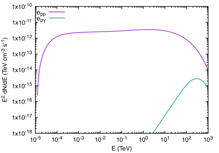
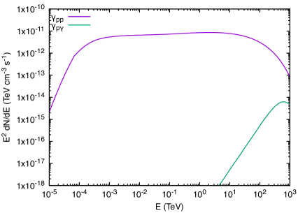
Figure 19: Comparison of the electron (top) and photon (bottom) emissivities for proton-proton and proton-photon interactions. Conditions appropriate for the stagnation point of the WCR are assumed, including a thermal proton number density of $3.9\times 10^{5}\,{\rm cm^{-3}}$ and a solid angle of $10^{-6}$ steradian for the disk of the O-star.

Appendix E Synchrotron emission

The synchrotron power per unit energy radiated by a single electron of energy $E_{\rm e}$ in a vacuum is given by (e.g. Ginzburg & Syrovatskii, 1965; Vila, 2012)

$$P_{\rm sync}(E_{\gamma},E_{\rm e},\alpha)=\frac{\sqrt{3}e^{3}B}{m_{\rm e}c^{2}h}\frac{E_{\gamma}}{E_{\rm c}}\int^{\infty}_{E_{\gamma}/E_{\rm c}}K_{5/3}(\zeta){\rm d}\zeta,$$ (46)

where $E_{\gamma}$ is the energy of the emitted photon and $K_{5/3}(\zeta)$ is a modified Bessel function of the second kind. $P_{\rm sync}$ peaks sharply near the characteristic energy

$$E_{\rm c}=\frac{3heB\sin\alpha}{4\pi m_{\rm e}c}\gamma_{\rm e}^{2},$$ (47)

where $\gamma_{\rm e}$ is the electron Lorentz factor, and the pitch angle $\alpha$ is the angle between the magnetic field (with flux density $B$) and the particle’s momentum. For a turbulent/isotropic magnetic field, $\sin\alpha=\sqrt{2/3}$. The integral in Eq. 46 can be approximated as (Melrose, 1980)

$$x\int^{\infty}_{x}K_{5/3}(\zeta){\rm d}\zeta\approx 1.85x^{1/3}e^{-x},$$ (48)

where $x=E_{\gamma}/E_{\rm c}$ is the dimensionless energy.

The situation changes somewhat if instead the electron is in the presence of a cold background plasma. In such a case the refractive index of the medium, which is smaller than unity, reduces the beaming effect, and can greatly reduce the synchrotron emission. This effect is know as the Tsytovitch-Razin effect (or, more generally, as the Razin effect; Tsytovitch, 1951; Razin, 1960). Eq. 46 now becomes (Ginzburg & Syrovatskii, 1965; Van Loo, Runacres & Blomme, 2004)

$$P_{\rm sync}(E_{\gamma},E_{\rm e},\alpha)=\frac{\sqrt{3}e^{3}B}{m_{\rm e}c^{2}h}f\frac{E_{\gamma}}{E_{\rm c}^{1}}\int^{\infty}_{E_{\gamma}/E_{\rm c}^{1}}K_{5/3}(\zeta){\rm d}\zeta,$$ (49)

where

$$f=\left(1+\frac{\nu_{0}^{2}}{\nu^{2}}\gamma_{\rm e}^{2}\right)^{-1/2},$$ (50)

$\nu_{0}=\sqrt{n_{\rm e}e^{2}/\pi m_{\rm e}}$ is the plasma frequency, and $n_{\rm e}$ is the number density of thermal electrons. $E_{\rm c}^{1}=f^{3}E_{\rm c}$.

Eq. 49 may be used for even mildly relativistic electrons, provided that $\chi=\nu/\nu_{\rm b}\mathrel{\hbox to0.0pt{\lower 3.0pt\hbox{$\sim$}\hss}\raise 2.0pt\hbox{$>$}}100$, where $\nu_{\rm b}=\omega_{\rm b}/2\pi$ and $\omega_{\rm b}=eB/m_{\rm e}c$ is the cyclotron frequency of the electron. To capture the transition from cyclotron to synchrotron emission, a data table of emissivity values for $1<\gamma<5$ and $10^{-2}<\chi<2\times 10^{3}$ is created using the approach given in Mahadevan et al. (1996).

The photon emission (photon s^-1 erg^-1) is then obtained from integrating over the volume and the distribution of non-thermal electrons:

$$q_{\rm sync}(E_{\gamma})=\frac{1}{E_{\gamma}}\int_{V}dV\sin\alpha\int_{E_{\rm e}^{\rm min}}^{E_{\rm e}^{\rm max}}N_{\rm e}(E_{\rm e})P_{\rm sync}(E_{\gamma},E_{\rm e},\alpha)dE_{\rm e},$$ (51)

where $N_{\rm e}$ is the distribution function of the non-thermal electrons (units of electrons cm^-3 erg^-1).

Appendix F Photon-photon absorption by pair creation

In CWB systems the stars provide large numbers of target photons for electron-positron pair production with high-energy ($\sim$ TeV) $\gamma$-rays. The probability of absorption depends on the cosine of the angle between the directions of the two photons, $\mu$. For a $\gamma$-ray of energy $E$ interacting with a stellar photon of energy $\epsilon$, the optical depth is given by

$$\frac{{\rm d}\tau}{{\rm d}\epsilon{\rm d}\Omega{\rm d}l}=(1-\mu)n_{\rm ph}\sigma_{\gamma\gamma},$$ (52)

where ${\rm d}l$ is the distance along the path of the $\gamma$-ray, ${\rm d}\Omega$ is the solid angle of the stellar surface, and $n_{\rm ph}$ is the radiation density which is assumed to be that of a blackbody of temperature $T_{*}$:

$$n_{\rm ph}=\frac{2\epsilon^{2}}{h^{3}c^{3}}\frac{1}{{\rm exp}(\epsilon/(kT_{*}))-1}\hskip 28.45274pt{\rm(ph\,cm^{-3}\,erg^{-1}\,sr^{-1})}.$$ (53)

The cross-section depends only on $\beta=(1-1/s)^{1/2}$, where $s=\epsilon/\epsilon_{\rm min}$ and the threshold energy

$$\epsilon_{\rm min}=\frac{2m_{\rm e}^{2}c^{4}}{E(1-\mu)}.$$ (54)

The cross-section is (Gould & Schréder, 1967)

$$\sigma_{\gamma\gamma}(\beta)=\frac{3}{16}\sigma_{\rm T}(1-\beta^{2})\left[(3-\beta^{4}){\rm ln}\left(\frac{1+\beta}{1-\beta}\right)-2\beta(2-\beta^{2})\right].$$ (55)

We follow the prescription given in Dubus (2006) to calculate the opacity (see also Romero, del Valle & Orellana, 2010). The integral over solid angle can be split into one over $\mu$ and $\phi$. As noted by Dubus (2006), the energy integral can be replaced with a definite integral over $\beta$ between the limits [0,1] while the integral along $l$ can be replaced with a definite integral over the angle $\psi$ between the limits [$\psi_{0},\pi$]. The final equation for calculating the optical depth then becomes

$$\tau=\int_{\psi_{0}}^{\pi}\frac{d_{0}\sin\psi_{0}}{\sin^{2}\psi}{\rm d}\psi\int_{\mu_{\rm min}}^{1}{\rm d}\mu\int_{0}^{2\pi}{\rm d}\phi\\ \times\int_{0}^{1}\frac{2\epsilon^{2}\sqrt{1-\beta}}{\epsilon_{\rm min}}(1-\mu)n_{\rm ph}\sigma_{\gamma\gamma}{\rm d}\beta,$$ (56)

where $\mu_{\rm min}=(1-R_{*}^{2}/d^{2})^{1/2}$ and $d$ is the distance of the $\gamma$-ray to the star.

Appendix G Free-free absorption

The emission from the WCR can also be absorbed by the stellar winds. In our axisymmetric model, the line of sight to the observer from a given patch on the WCR may pass solely through the primary or secondary wind, or it may pass first through the secondary wind and then move into the primary wind.

The dot product of the line of sight vector with the normal to the shock determines if the line of sight moves into the primary wind or into the secondary wind. If the latter occurs the line of sight may remain in the secondary wind, or it may intersect another part of the WCR and then move into the primary wind. To determine if this latter case occurs, a triangle or quadrangle facet is constructed from each patch on the WCR. Triangular facets are constructed only for those patches that touch the apex of the WCR, while quadrangles are constructed for all other patches. The list of triangle and quadrangle facets is then run through to find intersections with the line of sight, using standard techniques (Schlick & Subrenat, 1993; Möller & Trumbore, 1997).

For an ionized stellar wind consisting solely of protons and electrons the optical depth due to free-free absorption along a line of sight, $s$, is given by (see Wright & Barlow, 1975; Panagia & Felli, 1975)

$${\rm d}\tau=\int_{s_{0}}^{s_{1}}n^{2}K{\rm d}s=n_{0}^{2}K\int_{s_{0}}^{s_{1}}\frac{{\rm d}s}{s^{2}+q^{2}}=\frac{n_{0}^{2}K}{2q^{3}}\left[\frac{qs}{d^{2}}+\tan^{-1}\left(\frac{s}{q}\right)\right]_{s_{0}}^{s_{1}}.$$ (57)

Here the proton (and electron) number density is

$$n=\frac{n_{0}}{s^{2}+q^{2}},$$ (58)

with

$$n_{0}=\frac{\hbox{${\dot{M}}$}}{4\pi\hbox{${v_{\infty}}$}\,m_{\rm H}}.$$ (59)

The line of sight ray has an impact parameter $q$ with the star, $s=0$ at the point of closest approach to the star, and the observer is at $s=+\infty$. In Eq. 57, $s_{0}$ is the starting point of the ray and $s_{1}$ is either equal to $+\infty$ or the value obtained at the intersection point of the WCR. In the latter case the total opacity is obtained from $\tau=d\tau_{1}+d\tau_{2}$, where $d\tau_{1}$ and $d\tau_{2}$ are the optical depths through each wind along the line of sight.

In cgs units, $K$ is given by (Wright & Barlow, 1975)

$$K=3.7\times 10^{8}[1-\exp(-h\nu/kT)]g(\nu,T)T^{-1/2}\nu^{-3}\hskip 14.22636pt{\rm cm^{5}},$$ (60)

where $g$ is the Gaunt factor. $K$ is appropriately scaled for a wind with other atomic species. In evaluating $K$ we assume that the wind temperature is maintained at $10^{4}$ K. Hydrogen and helium are assumed to be singly ionized while C, N and O are assumed to be doubly ionized. The relative number densities of H, He and CNO are assumed to be given by $X$, $Y/4$ and $Z/14.24$. Finally, if the wind is clumpy, Eq. 57 is scaled by $1.0/f$, where $f$ is the volume filling factor of the clumps ($f<1.0$).

Additional absorption due to the material in the WCR can also be included, if desired (see, e.g., Parkin & Pittard, 2008). However, this addition is only likely to be significant if the WCR strongly cools, and so is not included in the present work.

References

- Amato & Blasi (2005) Amato E., Blasi P., 2005, MNRAS, 364, L76
- Amato & Blasi (2006) Amato E., Blasi P., 2006, MNRAS, 371, 1251
- Atoyan & Dermer (2003) Atoyan A.M., Dermer C.D., 2003, ApJ, 586, 79
- Bednarek (2005) Bednarek W., 2005, MNRAS, 363, L46
- Bell (1978) Bell A.R., 1978, MNRAS, 182, 147
- Bell et al. (2013) Bell A.R., Schure K.M., Reville B., Giacinti G., 2013, MNRAS, 431, 415
- Benaglia et al. (2020) Benaglia P., De Becker M., Ishwara-Chandra C.H., Intema H., Isequilla N.L., 2020, PASA, 37, 30
- Benaglia et al. (2015) Benaglia P., Marcote B., Moldón J., Nelan E., De Becker M., Dougherty S.M., Koribalski B.S., 2015, A&A, 579, A99
- Blasi (2002) Blasi P., 2002, Astropart. Phys., 16, 429
- Blasi et al. (2005) Blasi P., Gabici S., Vannoni G., 2005, MNRAS, 361, 907
- Blasi et al. (2007) Blasi P., Amato E., Caprioli D., 2007, MNRAS, 375, 1471
- Blomme et al. (2013) Blomme R., et al., 2013, A&A, 550, A90
- Blomme et al. (2017) Blomme R., Fenech D.M., Prinja R.K., Pittard J.M., Morford J.C., 2017, A&A, 608, A69
- Blumenthal & Gould (1970) Blumenthal G.R., Gould R.J., 1970, Rev. Mod. Phys., 42, 237
- Brookes (2016) Brookes D.P., 2016, PhD thesis, The University of Birmingham
- Bykov et al. (2014) Bykov A.M., Ellison D.C., Osipov S.M., Vladimirov A.E., 2014, ApJ, 789, 137
- Cantó et al. (1996) Cantó J., Raga A.C., Wilkin F.P., 1996, ApJ, 469, 729
- Caprioli et al. (2009) Caprioli D., Blasi P., Amato E., Vietri M., 2009, MNRAS, 395, 895
- Caprioli et al. (2010) Caprioli D., Kang H., Vladimirov A.E., Jones T.W., 2010, MNRAS, 407, 1773
- Caprioli et al. (2015) Caprioli D., Pop A.-R., Spitovsky A., 2015, ApJL, 798, L28
- Caprioli & Spitovsky (2014) Caprioli D., Spitovsky A., 2014, ApJ, 783, 91
- Caprioli et al. (2018) Caprioli D., Zhang H., Spitovsky A., 2018, Journal of Plasma Physics, 84, 715840301
- Corcoran et al. (2010) Corcoran M.F., Hamaguchi K., Pittard J.M., Russell C.M.P., Owocki S.P., Parkin E.R., Okazaki A., 2010, ApJ, 725, 1528
- De Becker et al. (2017) De Becker M., Benaglia P., Romero G.E., Peri C.S., 2017, A&A, 600, A47
- De Becker & Raucq (2013) De Becker M., Raucq F., 2013, A&A, 558, A28
- Decker (1988) Decker R.B., 1988, Space Sci. Rev., 48, 195
- del Palacio et al. (2016) del Palacio S., Bosch-Ramon V., Romero G., Benaglia P., 2016, A&A, 591, 139
- del Palacio et al. (2020) del Palacio S., et al., 2020, MNRAS, 494, 6043
- Dougherty et al. (2005) Dougherty S.M., Beasley A.J., Claussen M.J., Zauderer B.A., Bolingbroke N.J., 2005, ApJ, 623, 447
- Dougherty et al. (2003) Dougherty S.M., Pittard J.M., Kasian L., Coker R.F., Williams P.M., Lloyd H.M., 2003, A&A, 409, 217
- Dougherty & Pittard (2006) Dougherty S.M., Pittard J.M., 2006, in Proc. of the 8th European VLBI Network Symp., 49
- Dougherty et al. (2000) Dougherty S.M., Williams P.M., Pollacco D.L., 2000, MNRAS, 316, 143
- Dougherty et al. (1996) Dougherty S.M., Williams P.M., van der Hucht K.A., Bode M.F., Davis R.J., 1996, MNRAS, 280, 963
- Dubus (2006) Dubus G., 2006, A&A, 451, 9
- Eenens & Williams (1994) Eenens P.R.J., Williams P.M., 1994, MNRAS, 269, 1082
- Eichler & Usov (1993) Eichler D., Usov V., 1993, ApJ, 402, 271
- Ellison et al. (2004) Ellison D.C., Decourchelle A., Ballet J., 2004, A&A, 413, 189
- García-Segura (1997) García-Segura G., 1997, ApJ, 489, L189
- Giacalone (2005) Giacalone J., 2005, ApJ, 624, 765
- Ginzburg & Syrovatskii (1964) Ginzburg V., Syrovatskii S., 1964, “The Origin of Cosmic Rays” (New York: Macmillan)
- Ginzburg & Syrovatskii (1965) Ginzburg V., Syrovatskii S., 1965, ARA&A, 3, 297
- Gould & Schréder (1967) Gould R.J., Schréder G.P., 1967, Phys. Rev., 155, 1404
- Grevesse et al. (2010) Grevesse N., Asplund M., Sauval A.J., Scott P., 2010, Astrophys. Space Sci., 328, 179
- Grimaldo et al. (2019) Grimaldo E., Reimer A., Kissmann R., Niederwanger F., Reitberger K., 2019, ApJ, 871, 55
- Haggerty & Caprioli (2019) Haggerty C.C., Caprioli D., 2019, ApJ, 887, 165
- Hales et al. (2017) Hales C.A., Benaglia P., del Palacio S., Romero G.E., Koribalski B.S., 2017, A&A, 598, A42
- Hamaguchi et al. (2007) Hamaguchi K., et al., 2007, ApJ, 663, 522
- Hamaguchi et al. (2014a) Hamaguchi K., et al., 2014a, ApJ, 784, 125
- Hamaguchi et al. (2014b) Hamaguchi K., et al., 2014b, ApJ, 795, 119
- Hamaguchi et al. (2016) Hamaguchi K., et al., 2016, ApJ, 817, 23
- Hamaguchi et al. (2018) Hamaguchi K., et al., 2018, Nature Astronomy, 2, 731
- Henley et al. (2008) Henley D. B., Corcoran M. F., Pittard J. M., Stevens I. R., Hamaguchi K., Gull T. R., 2008, ApJ, 680, 705
- H.E.S.S. collaboration (2020) H.E.S.S. Collaboration, Abdalla et al., 2020, A&A, 635, A167
- Hillas (1984) Hillas A.M., 1984, ARA&A, 22, 425
- Hussein & Shalchi (2014) Hussein M., Shalchi A., 2014, ApJ, 785, 31
- Jones & Ellison (1991) Jones F.C., Ellison D.C., 1991, Space Sci. Rev., 58, 259
- Kato (2015) Kato T.N., 2015, ApJ, 802, 115
- Khangulyan et al. (2008) Khangulyan D., Aharonian F.A., Bosch-Ramon V., 2008, MNRAS, 383, 467
- Khangulyan et al. (2014) Khangulyan D., Aharonian F.A., Kelner S.R., 2014, ApJ, 783, 100
- Kelner et al. (2006) Kelner S.R., Aharonian F.A., Bugayov V.V., 2006, Phys. Rev. D, 74, 034018
- Kelner & Aharonian (2008) Kelner S.R., Aharonian F.A., 2008, Phys. Rev. D, 78, 034013
- Lagage & Cesarsky (1983) Lagage P.O, Cesarsky C.J., 1983, A&A, 125, 249
- Lépine et al. (2001) Lépine S., Wallace D., Shara M.M., Moffat A.F.J., Niemela V.S., 2001, AJ, 122, 3407
- Longair (1994) Longair M.S., 1994, High Energy Astrophysics. Vol. 2, 2nd edn., Cambridge Univ. Press, Cambridge
- Mannheim & Schlickeiser (1994) Mannheim K., Schlickeiser R., 1994, A&A, 286, 983
- Mahadevan et al. (1996) Mahadevan R., Narayan R., Yi I., 1996, ApJ, 465, 327
- Melrose (1980) Melrose D.B., 1980, Plasma astrophysics: Nonthermal processes in diffuse magnetized plasmas, Astrophysical applications (New York, Gordon and Breach Science Publishers), 2, 430
- Möller & Trumbore (1997) Möller T., Trumbore B., 1997, Journal of Graphics Tools, 2, 21
- Morlino & Caprioli (2012) Morlino G., Caprioli D., 2012, A&A, 538, A81
- Mücke et al. (2000) Mücke A., Engel R., Rachen J.P., Protheroe R.J., Stanev T., 2000, Comput. Phys. Commun., 124, 290
- Nakamura et al. (2010) Nakamura K., et al., 2010, J. Phys. G Nucl. Partic., 37, 075021
- Niemela et al. (1998) Niemela V.S., Shara M.M., Wallace D.J., Zurek D.R., Moffat A.F.J., 1998, AJ, 115, 2047
- Nugis & Lamers (2000) Nugis T., Lamers H.J.G.L.M., 2000, A&A, 360, 227
- O’Connor et al. (2005) O’Connor E.P., Dougherty S.M., Pittard J.M., Williams P.M., 2005, in Massive Stars and High-Energy Emission in OB Associations, eds. G. Rauw, Y. Nazé, R. Blomme, & E. Gosset, 81
- Orellana et al. (2007) Orellana M., Bordas P., Bosch-Ramon V., Romero G., Paredes J.M., 2007, A&A, 476, 9
- Ortiz-León et al. (2011) Ortiz-León G., Loinard L., Rodríguez L.F., Mioduszewski A.J., Dzib S.A., 2011, ApJ, 737, 30
- Panagia & Felli (1975) Panagia N., Felli M., 1975, A&A, 39, 1
- Park et al. (2015) Park J., Caprioli D., Spitkovsky A., 2015, Phys. Rev. Lett., 114, 085003
- Parkin & Gosset (2011) Parkin E. R., Gosset E., 2011, A&A, 530, A119
- Parkin & Pittard (2008) Parkin E. R., Pittard J.M., 2008, MNRAS, 388, 1047
- Parkin et al. (2011) Parkin E. R., Pittard J. M., Corcoran M. F., Hamaguchi K., 2011, ApJ, 726, 105
- Parkin et al. (2014) Parkin E. R., Pittard J. M., Nazé Y., Blomme R., 2014, A&A, 570, A10
- Pittard (2009) Pittard J.M., 2009, MNRAS, 396, 1743
- Pittard & Dawson (2018) Pittard J.M., Dawson B., 2018, MNRAS, 477, 5640
- Pittard & Dougherty (2006) Pittard J.M., Dougherty S.M., 2006, MNRAS, 372, 801
- Pittard et al. (2006) Pittard J.M., Dougherty S.M., Coker R.F., O’Connor E., Bolingbroke N.J., 2006, A&A, 446, 1001
- Pittard & Parkin (2010) Pittard J.M., Parkin E.R., 2010, MNRAS, 403, 1657
- Pittard et al. (2020) Pittard J.M., Vila G.S., Romero G.E., 2020, MNRAS, 495, 2205
- Pollock et al. (2005) Pollock A. M. T., Corcoran M. F., Stevens I. R., Williams P. M., 2005, ApJ, 629, 482
- Pshirkov (2016) Pshirkov M.S., 2016, MNRAS, 457, L99
- Rate & Crowther (2020) Rate G., Crowther P.A., 2020, MNRAS, 493, 1512
- Razin (1960) Razin V.A., 1960, Radiophysica, 3, 584
- Reitberger et al. (2015) Reitberger K., Reimer A., Reimer O., Takahashi H., 2015, A&A, 577, A100
- Reville & Bell (2013) Reville B., Bell A.R., 2013, MNRAS, 430, 2873
- Romero et al. (2010) Romero G.E., del Valle M.V., Orellana M., 2010, A&A, 518, A12
- Schlick & Subrenat (1993) Schlick C., Subrenat G., 1993, “Ray Intersection of Tessellated Surfaces: Quadrangles versus Triangles”, Graphics Gems V, Academic Press, p232
- Stage et al. (2006) Stage M.D., Allen G.E., Houck J.C., Davis J.E., 2006, Nature Physics, 2, 614
- Stevens et al. (1992) Stevens I.R., Blondin J.M., Pollock A.M.T., 1992, ApJ, 386, 265
- Sugawara et al. (2015) Sugawara Y., et al., 2015, PASJ, 67, 121
- Tsytovitch (1951) Tsytovitch V.N., 1951, Vest. Mosk. Univ., 11, 27
- Vacca et al. (1996) Vacca W.D., Garmany C.D., Shull J.M., 1996, ApJ, 460, 914
- Van Loo et al. (2004) Van Loo S., Runacres M.C., Blomme R., 2004, A&A, 418, 717
- van Marle et al. (2018) van Marle A.J., Casse F., Marcowith A., 2018, MNRAS, 473, 3394
- Vainio & Schlickeiser (1999) Vainio R., Schlickeiser R., 1999, A&A, 343, 303
- Vila (2012) Vila G.S., 2012, PhD thesis “Radiative models for jets in X-ray binaries”, Universidad de Buenos Aires
- Werner et al. (2013) Werner M., Reimer O., Reimer A., Egberts K., 2013, A&A, 555, A102
- White et al. (2020) White R., Breuhaus M., Konno R., Ohm S., Reville B., Hinton J.A., 2020, A&A, 635, A144
- Williams et al. (1997) Williams P.M., Dougherty S.M., Davis R.J., van der Hucht K.A., Bode M.F., Setia Gunawan D.Y.A., 1997, MNRAS, 289, 10
- Willis et al. (1997) Willis A.J., Dessart L., Crowther P.A., Morris P.W., van der Hucht K.A., 1997, Ap&SS, 255, 167
- Wright & Barlow (1975) Wright A.E., Barlow M.J., 1975, MNRAS, 170, 41
- Xu et al. (2020) Xu R., Spitkovsky A., Caprioli D., 2020, ApJL, 897, L41
- Zhekov (2017) Zhekov S.A., 2017, MNRAS, 472, 4374