SIRSi-Vaccine dynamical model for Covid-19 pandemic

Abstract

The Severe Acute Respiratory Syndrome Corona Virus 2 (SARS-CoV-2), or Covid-19, burst into a pandemic in the beginning of 2020. An unprecedented worldwide effort involving academic institutions, regulatory agencies and industry is facing the challenges imposed by the rapidly spreading disease. Emergency use authorization for vaccines were granted in the beginning of December 2020 in Europe and nine days later in the United States. The urge for vaccination started a race, forcing governs and health care agencies to take decisions on the fly regarding the vaccination strategy and logistics. So far, the vaccination strategies and non-pharmaceutical interventions, such as social distancing and the use of face masks, are the only efficient actions to stop the pandemic. In this context, it is of fundamental importance to understand the dynamical behavior of the Covid-19 spread along with possible vaccination strategies. In this work a Susceptible - Infected - Removed - Sick with vaccination (SIRSi-Vaccine) model is proposed. In addtion, the SIRSi-Vaccine model also accounts for unreported, or asymptomatic, cases and the possibility of temporary immunity, either after infection or vaccination. Disease free and endemic equilibrium points existence conditions are determined in the ($\omega\times\theta$) vaccine-effort and social distancing parameter space. The model is adjusted to the data from São Paulo, Santos and Campinas, three major cities in the State of São Paulo, Brazil.

1 Introduction

In 30 January 2020 the World Health Organization (WHO) declared a Public Health Emergency of International Concern (PHEIC). Four weeks before, the Wuhan Municipal Health Commission had reported a cluster of pneumonia cases, whose causative agent was soon after discovered to be the Severe Acute Respiratory Syndrome Corona Virus 2 (SARS-CoV-2), or Covid-19. Despite the WHO alert, the Covid-19 became pandemic weeks later, in March 2020 [1, 2].

It is of great concern the fact that worldwide governs and Health Care Agencies were unable to stop the Covid-19 pandemic in its beginning. As a result, the rapidly spreading disease is challenging health care angencies, academic institutions and industry to develop and deploy efficient drug treatments and vaccination.

A number of drugs have been tried in patients with Covid-19 disease. Unfortunately, studies [3, 4, 5, 6, 7] found that the drugs had little or no effect on the overall mortality, initiation of ventilation, duration of hospital stay or viral clearance even for patients with chronic use of some of the tried drugs.

On the other hand, non-pharmaceutical interventions (NPI), such as physical distancing, use of face masks and eye protection, reduce the virus transmission [8, 9]. Worldwide populations have been compliant to NPI, however, in some countries, there is a controversy over its effectiveness [10]. In Brazil, the closure of non-essential activities lasted only for a short time, and the cities lifted NPI in an uncoordinated manner [9]. As a result, in the beginning of November 2020, the downward trend reversed and the number of Covid-19 cases started to raise in a second wave of infection [11].

The development of vaccines usually takes many years, even decades, and is also very expensive. The fast development of Covid-19 vaccines was only possible since researchers had been working for years on vaccines for similar viruses, such as, SARS (Severe Acute Respiratory Syndrome) and MERS (Middle East Respiratory Syndrome). In addition, the experience gained with the Ebola vaccine showed that the development of new vaccines can be accelerated with a worldwide effort, including academic institutions, industry and health care regulatory agencies, without compromising safety [12, 13, 14].

There are currently 78 vaccines in clinical trial on humans, and other 77 are under investigation in animals. Emergency use authorization for vaccines were granted in the beginning of December 2020 by Britain’s National Health Service, and later on by the U.S. Food and Drug Administration (FDA). In january 2021 the Brazilian national health surveillance agency (Anvisa) also granted emergency use for vaccines. Up to now, in several countries, 6 vaccines have been granted emergency use, and 7 approved for full use [15, 16].

The Covid-19 pandemic, and the consequent urge for vaccination, started a race, with countries trying to vaccinate populations as fast as possible. In [17] the immunization results of a nationwide mass vaccination in Israel is reported, strengthening the expectation of Covid-19 pandemic effects mitigation. However, at the current pace, and for most countries, a successful vaccination strategy consists of a long journey ahead [18].

Logistics plays an important role in vaccination strategies deployment, since the efficacy of the vaccines currently in development ranges from 50.38% to 95.0% [15], and that different vaccines need different vaccination strategies, given the number of doses, the number of weeks apart each dose, specific storage facility needs, and so on.

Besides, Health Care Agencies must take decisions considering the Covid-19 new variants, vaccination strategy with varying NPI adherence among the population, or consider to delay the second dose in order to speed up the one dose vaccinated population [19, 20]. In addition, important factors are vaccine efficacy and population vaccination cover. Vaccines have to have at least $70\%$ efficacy with population cover of $75\%$ to prevent a pandemic without any other intervention. To stop the ongoing pandemic the needed vaccines efficacy raises to at least $80\%$, for $75\%$ population cover [21].

Given such complex context it is important to understand the dynamical behavior of the Covid-19 pandemic, considering possible vaccination strategies in order to mitigate of even to extinguish the ongoing pandemic.

Many scientific works have been developed since the beginning of the pandemic, aiming to stop, or mitigate, the pandemic effects, consisting of control systems strategies, and deep learning modeling. Other works, consisting of mathematical modeling, analysis, and numerical simulations, in order to predict the Covid-19 contagious behavior, have also been published.

In [22] time-series models - Auto-Regressive Integrated Moving Average (ARIMA) and Seasonal Auto-Regressive Integrated Moving Average (SARIMA) are developed for the COVID-19 pandemic, with data for the countries where $70\%$ - $80\%$ of global cumulative cases are located. The results show exponential growth of confirmed cases and deaths. In [23] a two parameter model is used to predict the pandemic evolution in France.

A Susceptible - Infected - Removed model is used to predict the Covid-19 pandemic in Kuwait [24]. A SIR-type model with non-constant population is developed In [25]. The model is calibrated to the rates of infection and deaths for Italy, Spain and the USA.

In [26] the death toll due to the Covid-19 pandemic is modeled via sigmoid curve, predicting mortality, and estimating practical interest values such as the number of new cases per infection, i.e., the basic reproduction number.

In [27] a mathematical model of Covid-19 is developed. A control system is proposed aiming to reduce the number of the susceptible individuals in a population applying NPI consisting of social distancing.

A number of works consider deep learning to predict the number of Covid-19 cases. In [28] a prediction model of confirmed and death cases of Covid-19 is developed, based on a deep learning algorithm with two long short-term memory layers, considering the available data for Covid-19 in India. In [29], multilayer deep learning models with perceptron, random forest and Long short-term memory, are trained and used to forecast the Covid-19 pandemic in Iran.

In [30] a Susceptible - Infected - Removed - Sick (SIRSi) model is proposed, modeling unreported or asymptomatic cases, and considering the effects of temporary acquired immunity on the Covid-19 spread.

In this work, the model proposed in [30] is modified, and a vaccination strategy is included, consisting of a vaccination rate of susceptible individuals. The proposed SIRSi-Vaccine model is composed of four compartments, namely, Susceptible, Infected, Sick and Recovered. The focus is to assess the effects of vaccination associated with social distancing as a NPI in the Covid-19 spread dynamics.

The proposed SIRSi-Vaccine model presents both disease free and endemic equilibrium points. The equilibrium points stabilities are studied both analytically and numerically, and, as a result, the found equilibrium existence condition relates the effects of the social distancing to the vaccination rate.

In addition, the SIRSi-Vaccine model is numerically adjusted to the epidemic situation in São Paulo, Santos and Campinas, three major cities in the State of São Paulo connecting the shores with the interior of the São Paulo state. The numerical results show that in order to stop the Covid-19 spread different strategies may be necessary for different cities, concerning social distancing NPI and vaccination rates.

The paper is organized as follows; Section 2 presents the mathematical model. In Section 3 the equilibrium points are determined and their stability are investigated. The parametric fitting is presented in Section 4. In Section 5 the simulations results for São Paulo, Santos and Campinas are presented. The final remarks are shown in Section 6.

2 SIRSi and SIRSi-Vaccine mathematical models

A constant population model with four compartments is proposed, see Fig. 1. The compartments are defined as: Susceptible $(S)$, Infected $(I)$, Infected symptomatic positive tested $(S_{ick})$ and Recovered $(R)$.

In Fig 1, $I$ is the infectious population compartment representing the population in the incubation stage, i.e., prior to the onset of symptoms. Transmission during this period has been reported in [31, 32, 33].

Figure 1: SIRSi model with constant population.

The infected population can be asymptomatic or symptomatic, and according to [34] the incubation period is assumed to be of 5.1 days. Infectiousness occur $12$ hours prior to the symptoms onset for the symptomatic. On the other hand, for those who are asymptomatic, the infectiousness is assumed to occur $4.6$ days after infection. The average time between infection and infectiousness is 6.5 days.

Those who are asymptomatic or do not develop severe symptoms, i.e., neither tested nor documented cases, are moved to the $R$ (Recovered) compartment after a $1/\beta_{1}$ period [30].

The incubation period for those who are sympotmatic is $1/\beta_{2}$. Once the infected individual is tested positive and the case is documented, it is moved to the $S_{ick}$ compartment, which consists of those patients with severe symptoms seeking medical attention.

After a period $1/\beta_{3}$ the $S_{ick}$ population that recovers is moved to the compartment $R$.

The possibility of temporary immunity for recovered individuals, as addressed in [35, 36, 37, 30], is also considered. As it can be seen in Fig. 1, the recovered $R$ population becomes susceptible $S$ again at a rate $\gamma$.

The model is developed considering the population size constraint of Eq. 1. In addition, the population growth and death rates $\mu$, including deaths due to Covid-19, are similar in the State of São Paulo [38], therefore, in this work, they are considered to be equal.

$$N=S(t)+I(t)+S_{ick}(t)+R(t)$$ (1)

From the foregoing considerations the SIRSi mathematical model is given by Eq. 2.

$$\begin{split}\frac{d}{dt}S(t)&=\mu N-\frac{\alpha(1-\theta)}{N}S(t)I(t)-\mu S(t)+\gamma R(t);\\ \frac{d}{dt}I(t)&=\frac{\alpha(1-\theta)}{N}S(t)I(t)-(\beta_{1}+\beta_{2})I(t)-\mu I(t);\\ \frac{d}{dt}S_{ick}(t)&=\beta_{2}I(t)-\beta_{3}S_{ick}(t)-\mu S_{ick}(t);\\ \frac{d}{dt}R(t)&=\beta_{1}I(t)+\beta_{3}S_{ick}(t)-\gamma R(t)-\mu R(t);\end{split}$$ (2)

In Eq. 2, the effect of social distancing measure, which is a form of NPI, is introduced by the parameter $\theta$, $0<\theta<1$. Where $\theta=0$ means that no social distancing measure is under consideration, and $\theta=1$ means a complete lockdown.

A normalization with respect to the population size $N$ is performed in Eq. 1, resulting in Eq. 3,

$$1=s(t)+i(t)+s_{ick}(t)+r(t)$$ (3)

where $s(t)=S(t)/N$, $i(t)=I(t)/N$, $s_{ick}(t)=S_{ick}(t)/N$ and $r(t)=R(t)/N$. Replacing Eq. 3 into the system of Eq. 2, results Eq. 4.

$$\begin{split}\frac{d}{dt}s(t)&=\mu-\alpha(1-\theta)si-\mu s+\gamma r;\\ \frac{d}{dt}i(t)&=\alpha(1-\theta)si-(\beta_{1}+\beta_{2})i-\mu i;\\ \frac{d}{dt}s_{ick}(t)&=\beta_{2}i-\beta_{3}s_{ick}-\mu s_{ick};\\ \frac{d}{dt}r(t)&=\beta_{1}i+\beta_{3}s_{ick}-\gamma r-\mu r;\end{split}$$ (4)

In addition, from Eq. 3, the recovered compartment $r(t)$ can be written as a linear combination of the other compartments (or state variables), as shown in Eq. 5,

$$r(t)=1-s(t)-i(t)-s_{ick}(t),$$ (5)

consequently, the solutions $\Omega=\{(s(t),i(t),s_{ick}(t))\in\mathbb{R}^{3}_{+}\,|\,s(t)+i(t)+s_{ick}(t)\leq 1\}$ of the system of Eq. 4 can be studied in the system of Eq. 6,

$$\begin{split}\frac{d}{dt}s(t)&=\mu+\gamma-\alpha(1-\theta)si-(\mu+\gamma)s-\gamma i-\gamma s_{ick}\\ \frac{d}{dt}i(t)&=\alpha(1-\theta)si-(\beta_{1}+\beta_{2}+\mu)i\\ \frac{d}{dt}s_{ick}(t)&=\beta_{2}i-(\beta_{3}+\mu)s_{ick}\end{split}$$ (6)

with reproduction basic number,

$$R_{0}=\dfrac{\alpha(1-\theta)}{\beta_{1}+\beta_{2}+\mu}.$$ (7)

A vaccination intervention is introduced consisting of susceptible individuals vaccinated at a rate $\omega$. The vaccinated individuals are considered to become instantaneously immune after vaccination, being moved to the recovered compartment. The proposed SIRSi-Vaccine model is shown in Fig. 2.

Including the vaccination intervention in Eqs. 4 and 6 results in Eqs. 8 and 9, respectively.

$$\begin{split}\frac{d}{dt}s(t)&=\mu-\alpha(1-\theta)si-\mu s+\gamma r-\omega s\\ \frac{d}{dt}i(t)&=\alpha(1-\theta)si-(\beta_{1}+\beta_{2})i-\mu i\\ \frac{d}{dt}s_{ick}(t)&=\beta_{2}i-\beta_{3}s_{ick}-\mu s_{ick}\\ \frac{dr}{dt}r(t)&=\beta_{1}i+\beta_{3}s_{ick}-\gamma r+\omega s-\mu r\end{split}$$ (8)

$$\begin{split}\frac{d}{dt}s(t)&=\mu+\gamma-\alpha(1-\theta)si-(\mu+\gamma+\omega)s-\gamma i-\gamma s_{ick}\\ \frac{d}{dt}i(t)&=\alpha(1-\theta)si-(\beta_{1}+\beta_{2}+\mu)i\\ \frac{d}{dt}s_{ick}(t)&=\beta_{2}i-(\beta_{3}+\mu)s_{ick}\end{split}$$ (9)

Figure 2: SIRSi model with vaccination intervention.

3 Disease-free and endemic equilibrium points

In this section the equilibrium points for the mathematical models in Eqs. 6 and 9 are determined and their stabilities are analysed.

3.1 SIRSi equilibrium points

The system of Eq. 6 has two equilibrium points, one is consistent with a disease-free situation, and the other representing an endemic equilibrium.

The disease-free equilibrium point $P_{df1}$ is given by Eq. 10.

$$P_{df1}=\left[\begin{array}[]{c}s^{\ast}\\ i^{\ast}\\ s^{\ast}_{ick}\end{array}\right]=\left[\begin{array}[]{c}1\\ 0\\ 0\end{array}\right]$$ (10)

On the other hand, the endemic equilibrium point $P_{e1}$ is given by Eq. 11

$$P_{e1}=\left[\begin{array}[]{c}s^{\ast}\\ i^{\ast}\\ s^{\ast}_{ick}\end{array}\right]=\left[\begin{array}[]{c}\frac{\beta_{1}+\beta_{2}+\mu}{\alpha\left(1-\theta\right)}\\ (\beta_{3}+\mu)\varphi\\ \beta_{2}\varphi\end{array}\right],$$ (11)

where

$$\varphi=\frac{\left(\gamma+\mu\right)\left(\alpha(1-\theta)-(\beta_{1}+\beta_{2}+\mu)\right)}{\alpha\left(1-\theta\right)\left((\beta_{1}+\beta_{2}+\mu)(\beta_{3}+\mu)+(\beta_{2}+\beta_{3}+\mu)\gamma\right)}.$$ (12)

In order to analyze the local stability of the point, the Jacobian matrix $J$ of the system in Eq. 6 is shown in Eq. 13.

$$J=\left[\begin{array}[]{@{}c@{}c@{}c@{}}-\alpha(1-\theta)i^{\ast}-(\mu+\gamma)&-\alpha(1-\theta)s^{\ast}-\gamma&-\gamma\\ \alpha(1-\theta)i^{\ast}&\alpha(1-\theta)s^{\ast}-(\beta_{1}+\beta_{2}+\mu)&0\\ 0&\beta_{2}&-(\beta_{3}+\mu)\end{array}\right]$$ (13)

The eigenvalues associated with $P_{df1}$, the disease free equilibrium point, are given by Eq. 14.

$$\begin{split}\lambda_{1}&=-(\mu+\gamma)\\ \lambda_{2}&=\alpha(1-\theta)-(\beta_{1}+\beta_{2}+\mu)\\ \lambda_{3}&=-(\beta_{3}+\mu)\end{split}$$ (14)

The eigenvalue $\lambda_{2}$ shows the possibility of a bifurcation since it can change sign depending on the parameters values. Therefore, the disease free equilibrium point $P_{df1}$ is stable if

$$\alpha(1-\theta)<\beta_{1}+\beta_{2}+\mu.$$ (15)

Comparing Eqs. 7 and Eq. 15 it can be noticed that if $R_{0}<1$ then $P_{df1}$ is locally asymptotically stable. On the other hand, if $R_{0}>1$, then $P_{df1}$ is unstable.

Considering the endemic equilibrium point $P_{e1}$, Eqs. 11 and 12, and the Jacobian matrix, Eq. 13, the characteristic polynomial of $P_{e1}$ is given by Eq. 16, where the coefficients are given by Eq. 17.

$$\mathcal{P}_{e1}(\lambda)=\lambda^{3}+a_{1}\lambda^{2}+a_{2}\lambda+a_{3},$$ (16)

$$\begin{split}a_{1}&=\varphi\alpha(1-\theta)\left(\beta_{3}+\mu\right)+\beta_{3}+\gamma+2\mu\\ a_{2}&=\left(\beta_{3}+\mu\right)\left[\gamma+\mu+\varphi\alpha(1-\theta)\left(\beta_{1}+\beta_{2}+\beta_{3}+\gamma+2\mu\right)\right]\\ a_{3}&=\varphi\alpha\left(1-\theta\right)\left(\beta_{3}+\mu\right)\left(\begin{array}[]{@{}c@{}}\beta_{1}\beta_{3}+\beta_{1}\mu+\beta_{2}\beta_{3}+\beta_{2}\gamma\\ +\beta_{2}\mu+\beta_{3}\gamma+\beta_{3}\mu+\gamma\mu+\mu^{2}\end{array}\right)\end{split}$$ (17)

The coefficients $a_{1}$, $a_{2}$ and $a_{3}$, in Eq. 17, are positive real numbers if $\varphi>0$ (see Eq. 12). In this case, in order to determine whether the characteristic polynomial in Eq. 16 has unstable or stable roots the Routh-Hurwitz stability criterion [39] is used.

Consequently, the characteristic polynomial in Eq. 16 is stable if expression 18 holds.

$$b_{1}=a_{2}-\frac{a_{3}}{a_{1}}>0$$ (18)

The proof that expression 18 holds true demands some mathematical reasoning, which results in Eq. 19.

$$\begin{split}b_{1}&=\frac{1}{a_{1}}\left(\beta_{3}+\mu\right)\left[\varphi^{2}c_{1}^{2}c_{2}+\varphi c_{1}c_{3}+c_{4}\right],\end{split}$$ (19)

where

$$\begin{split}c_{1}&=\alpha(1-\theta),\\ c_{2}&=(\beta_{1}+\beta_{2})(\beta_{3}+\mu)+\beta_{3}^{2}+\beta_{3}\gamma+3\beta_{3}\mu+\gamma\mu+2\mu^{2},\\ c_{3}&=\beta_{1}\gamma+\beta_{1}\mu+\beta_{2}\mu+\beta_{3}^{2}+2\beta_{3}\gamma+4\beta_{3}\mu+\gamma^{2}+4\gamma\mu+4\mu^{2},\\ c_{4}&=\beta_{3}\gamma+\beta_{3}\mu+\gamma^{2}+3\gamma\mu+2\mu^{2}.\end{split}$$

The expression inside brackets in Eq. 19 is positive if $\varphi>0$. Consequently, for $\varphi>0$ the expression 18 holds true, and $P_{3}$ is asymptotically stable. In addition, as it can be seen in Eq. 12, $\varphi>0$ implies that $R_{0}>1$.

3.2 SIRSi-Vaccine equilibrium points

Similarly to what was found in Section 3.2, the SIRSi-Vaccine mathematical model of Eq. 9 has two equilibrium points, the first one is consistent with a disease-free situation, and the other with an endemic equilibrium.

The disease free equilibrium point of Eq. 9 is shown in Eq. 20, for $s^{\ast}>0$.

$$P_{df2}=\left[\begin{array}[]{c}s^{\ast}\\ i^{\ast}\\ s_{ick}^{\ast}\end{array}\right]=\left[\begin{array}[]{c}\frac{\mu+\gamma}{\mu+\gamma+\omega}\\ 0\\ 0\end{array}\right]$$ (20)

The endemic equilibrium point $P_{e2}$ is given by Eq. 21

$$P_{e2}=\left[\begin{array}[]{c}s^{\ast}\\ i^{\ast}\\ s_{ick}^{\ast}\end{array}\right]=\left[\begin{array}[]{c}\frac{\beta_{1}+\beta_{2}+\mu}{\alpha(1-\theta)}\\ (\beta_{3}+\mu)\psi\\ \beta_{2}\psi\end{array}\right],$$ (21)

where

$$\psi=\frac{\alpha(1-\theta)(\gamma+\mu)-\left(\beta_{1}+\beta_{2}+\mu\right)\,\left(\gamma+\mu+\omega\right)}{\alpha(1-\theta)((\beta_{1}+\beta_{2}+\gamma+\mu)(\beta_{3}+\mu)+\beta_{2}\,\gamma)}.$$ (22)

The local stability of the equilibrium points are determined with the Jacobian matrix shown in Eq. 23.

$$J=\left[\begin{array}[]{@{}c@{}c@{}c@{}}-\alpha(1-\theta)i^{\ast}-(\mu+\gamma+\omega)&-\alpha(1-\theta)s^{\ast}-\gamma&-\gamma\\ \alpha(1-\theta)i^{\ast}&\alpha(1-\theta)s^{\ast}-(\beta_{1}+\beta_{2}+\mu)&0\\ 0&\beta_{2}&-(\beta_{3}+\mu)\\ \end{array}\right]$$ (23)

The disease free equilibrium point $P_{df2}$ is associated with the eigenvalues $\lambda_{1}$, $\lambda_{2}$ and $\lambda_{3}$ in Eqs. 24, 25 and 26, respectively.

$$\lambda_{1} =-(\gamma+\mu+\omega)$$ (24)

$$\lambda_{2} =-(\beta_{1}+\beta_{2}+\mu)+\alpha(1-\theta)\dfrac{\mu+\gamma}{\mu+\gamma+\omega}$$ (25)

$$\lambda_{3} =-(\beta_{3}+\mu)$$ (26)

From Eq. 24 and 26 it can be seen that $\lambda_{1}$ and $\lambda_{3}$ are negative. However, $\lambda_{3}$ is negative only if the condition in 27 holds true.

$$\omega>\left(\frac{\alpha(1-\theta)}{\beta_{1}+\beta_{2}+\mu}-1\right)(\mu+\gamma)=\left(R_{0}-1\right)(\mu+\gamma)$$ (27)

Therefore, considering the foregoing relations, and if condition 27 holds, the point $P_{e2}$ is locally asymptotically stable.

Now, regarding the endemic equilibrium point $P_{e2}$, it exists only if the condition expressed in 28 holds true.

$$\omega\leq\left(\dfrac{\alpha(1-\theta)}{\beta_{1}+\beta_{2}+\mu}-1\right)(\mu+\gamma)=\left(R_{0}-1\right)(\mu+\gamma)$$ (28)

It is interesting to notice that the existence condition depends on the vaccination rate $\omega$. Besides, for $R_{0}<1$, $P_{e2}$ exists only for negative values of $\omega$, which is a case of no physical concern.

The stability of the endemic equilibrium point $P_{e2}$ is conditioned to parameters combinations, including the social distancing $(\theta)$ and the vaccination rate $(\omega)$ parameters. The mathematical reasoning to derive and prove such stability conditions is cumbersome, for that reason, numerical analysis is used to infer the stability of the point.

The simulations results presented in Section 5, show that if the disease free equilibrium point $P_{df2}$ is unstable, then the trajectories in the vicinity of $P_{e2}$ are stable. These results can be seen from the numerical analysis represented by the bifurcation graphs in Section 5.

4 SIRSi-Vaccine model parametric fitting

In this section, the parameters of the SIRSi model (Eq. 6) are numerically determined by parametric fitting using public available data covering a one year period of the Covid-19 pandemic, specifically, ranging from March, 2020 to March, 2021.

The SIRSi-Vaccine model considers the social distancing influence on the Covid-19 infectiousness. Recently, a number of works have reported that Covid-19 epidemiological models are strongly sensitive to social distancing index [40, 41, 34, 30].

The social distancing index is time-varying, presenting an oscillatory behavior with approximately 7-days period, a feature that impairs the numerical parametric adjustment of the SIRSi-Vaccine model.

In order to avoid numerical problems, the approach is to use a polynomial function adjusted to the social distancing data as the social distancing index. The data is obtained using privacy-protected mobile phone device location information available in SEADE [42] for São Paulo, Campinas and Santos.

For the least-squares parameters adjustment raw data was used for São Paulo. On the other hand, for Campinas and Santos, instead of the raw data, a 21-day moving average filter was used in order to smooth the data prior to the least-squares fitting. In spite of that, the filtered data preserves both monthly trend and general behavior. The social distancing index polynomial fitting results can be seen in Figs. 3, 4 and 5.

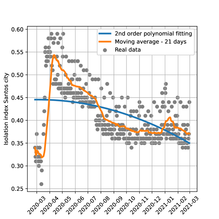
Figure 3: Isolation index of Santos.

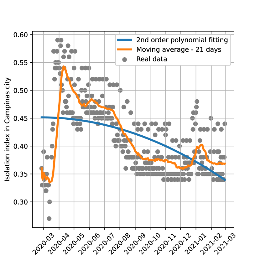
Figure 4: Isolation index of Campinas.

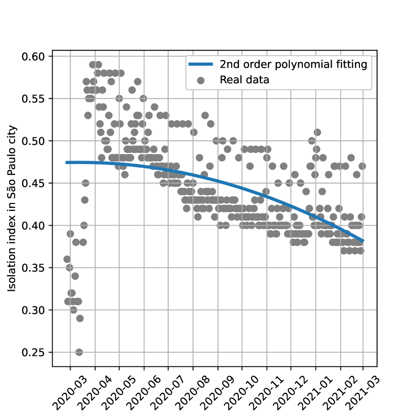
Figure 5: Isolation index of São Paulo.

For all the other parameters, the Least-squares Trust Region Reflective (TRR) algorithm [43, 44], which is a robust real-time optimization method, was used to fit the number of Covid-19 confirmed cases.

The free parameters in the fitting process are $\left(\gamma,\alpha,\beta_{1},\beta_{2},\beta_{3}\right)$ (see Fig. 2), and $s(0)$ which is the normalized amount of susceptible individuals prior the pandemic. The other normalized initial conditions are $s_{ick}(0)=0$ and $i(0)=1-s(0)$. In addition, for the lower and upper bounds of the parameters, epidemiological and clinical characteristics of Covid-19 reported in the literature where considered [45, 46, 47, 48]

The confirmed cases are considered to be the $s_{ick}(t)$ compartment population in the model of Eq. 9. The results of the least-squares TRR fitting comparing the confirmed cases and the respective $s_{ick}$ compartment simulation can be seen in Figs. 6, 7 and 8.

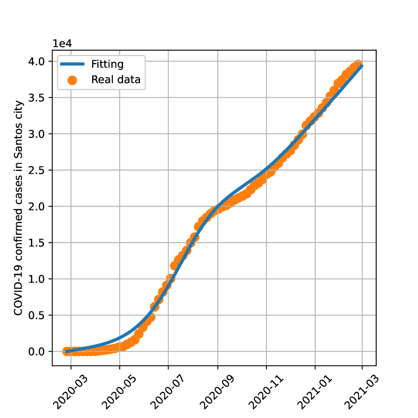
Figure 6: Covid-19 infection confirmed cases in Santos [38] compared to the respective $s_{ick}$ compartment.

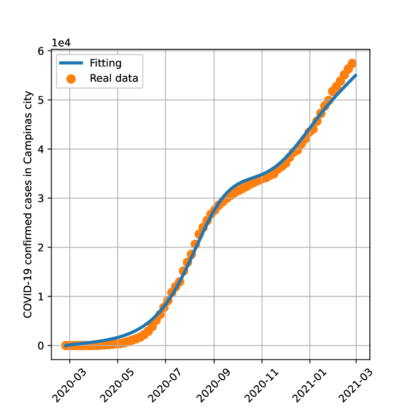
Figure 7: Covid-19 infection confirmed cases in Campinas [38] compared to the respective $s_{ick}$ compartment.

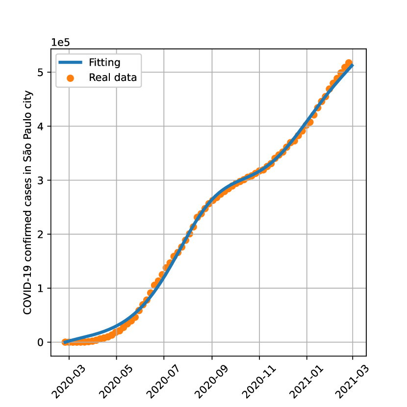
Figure 8: Covid-19 infection confirmed cases in São Paulo [38] compared to the respective $s_{ick}$ compartment.

The parameters determined with the least-squares TRR algorithm for Santos, Campinas, and São Paulo, are shown in the Tables 1, 2 and 3, respectively.

Parameter	Value
$\mu$	0.000027
$\gamma$	0.100000
$\alpha$	0.775985
$\theta$	0.415355
$\beta_{1}$	0.200000
$\beta_{2}$	0.200000
$\beta_{3}$	0.047847
$s_{0}$	0.999754
$i_{0}$	0.000246

Table 1: Fitted parameters for Santos.

Parameter	Value
$\mu$	0.000034
$\gamma$	0.038255
$\alpha$	0.776520
$\theta$	0.414454
$\beta_{1}$	0.200000
$\beta_{2}$	0.200000
$\beta_{3}$	0.067000
$s_{0}$	0.999883
$i_{0}$	0.000117

Table 2: Fitted parameters for Campinas.

Parameter	Value
$\mu$	0.000036
$\gamma$	0.032774
$\alpha$	0.811656
$\theta$	0.444603
$\beta_{1}$	0.200000
$\beta_{2}$	0.200000
$\beta_{3}$	0.058792
$s_{0}$	0.999800
$i_{0}$	0.000200

Table 3: Fitted parameters for São Paulo.

5 Simulation results

In this section, the numerical simulations of the SIRSi-Vaccine model (Eq. 9) are performed. The parameters used for the SIRSi-Vaccine model simulations are the same parameters determined for the SIRSi model in Section 4, and shown in Tables 1, 2 and 3.

In the simulations the social distancing index $\theta$ and the vaccination rate $\omega$ are kept constant over time. However, they are set up with different values in each performed simulation.

Two different scenarios are considered. Firstly, the vaccination rate is set to $\omega=0$, and the numerical simulations are performed for different values of the social distancing index, ranging from $\theta=0.0$, i.e., no social distancing intervention, to $\theta=0.7$ which means that $70$% of the population is locked home, keeping social distancing.

In the next scenario, the social distancing index $\theta$ is set up equal to the average value of the measured social distancing data. The values of $\theta$ used for each case can be seen in the Tables 1, 2 and 3. In this scenario, the simulations are performed considering different values of vaccination rate $\omega$ in order to assess the needed vaccination effort to stop, or, at least, to mitigate the spread of the Covid-19.

5.1 Simulation results for Santos

The simulations in Fig. 9 show that without vaccination the Covid-19 spread do not decay for a social distancing index less than $\theta=0.5$. On the other hand, for $\theta=0$ the number of cases nearly triple, which is a potential threath to health care units. With $\theta=0.7$ the infected population rapidly decay until the mid July, a behavior that is observed also for $\theta=0.5$, but slower in this last case.

It is important to point out that this hypothetical behavior offers an insight to what could be the result in such situation, since the social distancing data shows that $\theta$, in fact, presents a moving average value behavior combined with a 7-days periodic oscillation.

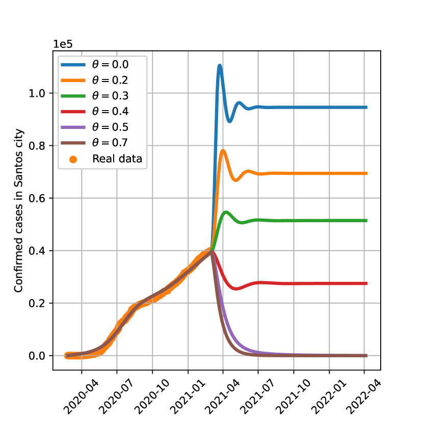
Figure 9: Simulation of infection confirmed cases for Santos with $\omega=0$ and different values of social distancing index.

The simulations in Fig. 10 are performed adopting constant social distancing index (see Table 1). As it can be seen, the simulations results are consistent with the equilibrium points stability and existing conditions in Section 3.2.

For the vaccination rate $\omega<0.1$ in Fig. 10, the disease free equilibrium point $P_{df2}$ is unstable according to condition 27, and the endemic equilibrium point $P_{e2}$ exists according to condition 28. The simulation also suggests that $P_{e2}$ is stable due to the steady number of confirmed cases over time.

For $\omega=0.1$ the situation is the opposite. In this case, the disease free point $P_{df2}$ is stable, and the endemic equilibrium point $P_{e2}$ does no exist, according to condition 28, and the number of confirmed cases decay to zero.

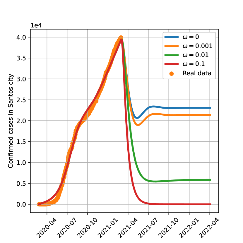
Figure 10: Simulation of infection confirmed cases for Santos considering different values of vaccination rate $\omega$.

In Fig. 11 the number of confirmed cases for Santos as a function of the social distancing index $\theta$ and of the vaccination rate $\omega$ is shown. In addition, Fig. 11 is also a bifurcation diagram, showing the stable region (dark-blue) in the parameter space of the disease free equilibrium point. The light-blue and green areas indicate the region where the disease free point is unstable. The same region indicates the existence of the endemic equilibrium.

Figure 11: Steady state response of the number of confirmed cases for Santos.

In addition, Fig. 11 shows the relation between the social distancing index $\theta$ and the vaccination rate $\omega$, indicating how to develop a vaccination strategy, combined with NPI for the city of Santos.

In this case, with an isolation index $\theta>0.5$ and a small vaccination rate, the number of confirmed cases decay to a disease free equilibrium. On the other hand, for $\theta<0.3$, the vaccination rate must be much higher, for instance $\omega>0.4$, otherwise the number of cases do not decay, remaining constant over time, in a situation compatible with an stable endemic equilibrium.

5.2 Simulation results for Campinas

The qualitative general behavior of the simulations for Campinas, shown in Figs. 12, 13 and 14, is similar to what is presented in the Section 5.1.

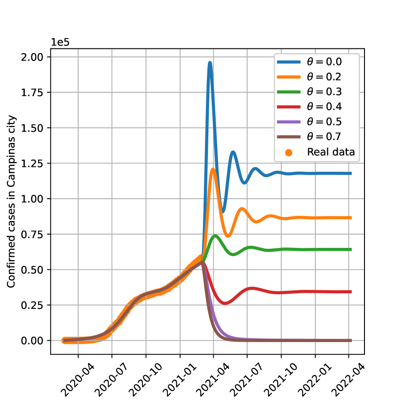
Figure 12: Simulation of infection confirmed cases for Campinas with $\omega=0$ and different values of social distancing index.

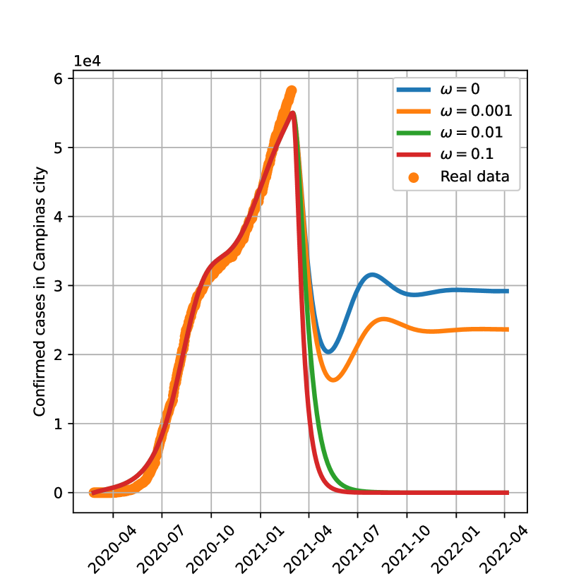
Figure 13: Simulation of infection confirmed cases for Campinas considering different values of vaccination rate $\omega$.

Figure 14: Steady state response of the number of confirmed cases for Campinas.

In Fig. 12 the number of confirmed cases is shown considering $\omega=0$, and for different values of social distancing index $\theta$.

As a result, it can be seen that for social distancing index higher than $0.5$, i.e, $\theta>0.5$, the disease free equilibrium is stable - condition 27 holds true - and the number of cases decay to zero over time.

Differently, for $\theta<0.5$, the disease free equilibrium is unstable. The endemic equilibrium exists - condition 28 holds true - and the number of cases do not decay over time. It is important to notice that for $\theta<0.3$ the number of confirmed cases abruptly increases, nearly quadrupling in a very short period. This indicates the importance of NPI to mitigate the Covid-19 spread and to prevent health care units from collapsing.

The simulations of infected confirmed cases for Campinas, considering a constant social distancing index $\theta$, see Table 2, and different values for the vaccination rate $\omega$, are shown in Fig. 13. In this case, a vaccination rate $\omega=0.1$ is enough to generate a stable disease free response. For smaller vaccination rates, however, the endemic equilibrium exists and the simulations suggests it is stable.

Comparing Figs. 11 and 14, the vaccination rate that is capable of generating stable disease free responses is considerably smaller for Campinas than for Santos. This behavior is probably due to the re-susceptibility feedback gain $\gamma$, since the value found for Santos is nearly $2.6$ times bigger than for Campinas, see Tables 1 and 2.

Another relevant information is the slightly bigger social distancing data dispersion for Santos, that influences on the infectiousness of the Covid-19 spread, and probably on the re-susceptibility feedback gain $\gamma$.

5.3 Simulation results for São Paulo

Again, for São Paulo, the qualitative general behavior of the simulations shown in Figs. 15, 16 and 17, is similar to the behavior of the simulations presented in the Sections 5.1 and 5.2.

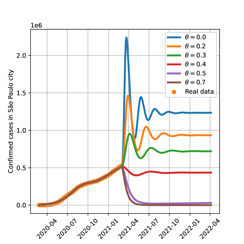
Figure 15: Simulation of infection confirmed cases for São Paulo with $\omega=0$ and different values of social distancing index.

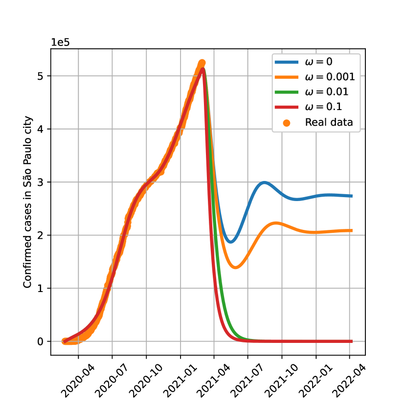
Figure 16: Simulation of infection confirmed cases for São Paulo considering different values of vaccination rate $\omega$.

Figure 17: Steady state response of the number of confirmed cases for São Paulo.

In Fig. 15 the simulations of the infection confirmed cases for $\omega=0$ and for different values of the social distancing index $\theta$ are shown. It can be seen that for $\theta>0.5$ the disease free equilibrium point is stable, i. e., condition 27 holds true, consequently the number of cases decay to zero over time.

On the other hand, for simulations with $\theta<0.5$ the disease free equilibrium is unstable, and since the condition 28 holds true, the endemic equilibrium exists. Therefore, the number of cases do not decay over time.

For $\theta<0.3$ the number of infection confirmed cases increases very fast, threatening the health care units of collapsing in a short period of time.

The simulations of infection confirmed cases shown in Fig. 16, indicate that for $\omega\geq 0.1$ the disease free equilibrium is stable. On the contrary, for the simulated values of $\omega<0.1$, the endemic equilibrium is stable while the disease free equilibrium is unstable. As a result, in this case, the number of infection confirmed cases do not decay over time.

Comparing Figs. 17, 14 and 11, it is clear that the simulation results obtained for São Paulo and Campinas are very similar concerning the behavior related to the social distancing index $\theta$ and the vaccination rate $\omega$. In order to stop the Covid-19 spread in Santos, the vaccination rate need to be higher.

The least-square fitting was performed differently for Campinas and Santos due to the dispersion of the social distancing index. The influence of this procedure is still not clear, and further investigation may be needed in order improve the SIRSi-Vaccine model response.

6 Conclusions

A compartmental model of the Covid-19 pandemic is proposed consisting of four compartments, namely: Susceptible - Infected - Recovered - Sick with vaccination (SIRSi-Vaccine), considering a vaccination strategy and the possibility of recovered patients become susceptible again, that is, individuals loose their acquired immunity either after recovery or vaccination.

The proposed SIRSi-Vaccine model has both disease free and endemic equilibrium points, presenting interchangeable stability, that is, the condition that assures stability for the disease free equilibrium imply the nonexistence of the endemic equilibrium. On the other hand, the endemic equilibrium existence condition imply on the instability of the disease free equilibrium. In addition, the existence and stability conditions of expressions 27 and 28 depend on both the reproduction basic number $R_{0}$ and on the vaccination rate $\omega$.

The proposed SIRSi-Vaccine model is least-squares fitted to Covid-19 pandemic publicly available data for Santos, Campinas and São Paulo. The qualitative general behavior of the simulations is compatible with the analytical results. However, comparing the simulations of Santos  with Campinas and São Paulo, a slightly different behavior is found for Santos.

The difference is probably due to the re-susceptibility feedback gain $\gamma$, determined by the least-squares algorithm, that is $2.6$ times higher for Santos, when compared with Campinas and São Paulo. This result indicates that for Santos, a successful vaccination strategy imply a higher vaccination rate.

Another result is the influence of the social distancing index $\theta$. Small variations on this index can generate abrupt increase in the number of infected confirmed Covid-19 cases in a short period of time. This behavior is of special concern due to the possible threat to health care units.

Availability of data and materials

Data are publicly available with [49, 38].

Declaration of competing interest

There is no conflict of interest between the authors.

References

- [1] A. Maxmen, Why did the world’s pandemic warning system fail when COVID hit?, Nature 589 (7843) (2021) 499–500. doi:10.1038/d41586-021-00162-4.
- [2] World Health Organization. WHO Timeline - COVID-19 [online] (Jun 2020) [cited 25 Jun 2020].
- [3] Repurposed antiviral drugs for covid-19 — interim WHO solidarity trial results, New England Journal of Medicine 384 (6) (2021) 497–511. doi:10.1056/NEJMoa2023184.
- [4] C. Johnston, E. R. Brown, J. Stewart, H. C. Karita, P. J. Kissinger, J. Dwyer, S. Hosek, T. Oyedele, M. K. Paasche-Orlow, K. Paolino, K. B. Heller, H. Leingang, H. S. Haugen, T. Q. Dong, A. Bershteyn, A. R. Sridhar, J. Poole, P. A. Noseworthy, M. J. Ackerman, S. Morrison, A. L. Greninger, M.-L. Huang, K. R. Jerome, M. H. Wener, A. Wald, J. T. Schiffer, C. Celum, H. Y. Chu, R. V. Barnabas, J. M. Baeten, Hydroxychloroquine with or without azithromycin for treatment of early sars-cov-2 infection among high-risk outpatient adults: A randomized clinical trial, EClinicalMedicine (2021) 100773 doi:10.1016/j.eclinm.2021.100773.
- [5] B. Tomlinson, S. P. Eftekhar, S. Kazemi, M. Barary, M. Javanian, S. Ebrahimpour, N. Ziaei, Effect of hydroxychloroquine and azithromycin on qt interval prolongation and other cardiac arrhythmias in covid-19 confirmed patients, Cardiovascular Therapeutics 2021 (2021) 6683098. doi:10.1155/2021/6683098.
- [6] L. M. Bush, A. K. Rahman, A. G. Purdy, P. T. Ender, Covid-19 pneumonia in patients on chronic hydroxychloroquine therapy: Three cases of covid-19 pneumonia, Case Reports in Infectious Diseases 2020 (2020) 8822753. doi:10.1155/2020/8822753.
- [7] P. R. Bignardi, C. S. Vengrus, B. M. Aquino, A. C. Neto, Use of hydroxychloroquine and chloroquine in patients with COVID-19: a meta-analysis of randomized clinical trials, Pathogens and Global Health (2021) 1–12. doi:10.1080/20477724.2021.1884807.
- [8] D. K. Chu, E. A. Akl, S. Duda, K. Solo, S. Yaacoub, H. J. Schünemann, D. K. Chu, E. A. Akl, A. El-harakeh, A. Bognanni, T. Lotfi, M. Loeb, A. Hajizadeh, A. Bak, A. Izcovich, C. A. Cuello-Garcia, C. Chen, D. J. Harris, E. Borowiack, F. Chamseddine, F. Schünemann, G. P. Morgano, G. E. U. Muti Schünemann, G. Chen, H. Zhao, I. Neumann, J. Chan, J. Khabsa, L. Hneiny, L. Harrison, M. Smith, N. Rizk, P. Giorgi Rossi, P. AbiHanna, R. El-khoury, R. Stalteri, T. Baldeh, T. Piggott, Y. Zhang, Z. Saad, A. Khamis, M. Reinap, S. Duda, K. Solo, S. Yaacoub, H. J. Schünemann, Physical distancing, face masks, and eye protection to prevent person-to-person transmission of sars-cov-2 and covid-19: a systematic review and meta-analysis, The Lancet 395 (10242) (2020) 1973–1987. doi:10.1016/S0140-6736(20)31142-9.
- [9] A. A. de Souza Santos, D. d. S. Candido, W. M. de Souza, L. Buss, S. L. Li, R. H. M. Pereira, C.-H. Wu, E. C. Sabino, N. R. Faria, Dataset on SARS-CoV-2 non-pharmaceutical interventions in Brazilian municipalities, Scientific Data 8 (1) (2021) 73. doi:10.1038/s41597-021-00859-1.
- [10] J. L. Scheid, S. P. Lupien, G. S. Ford, S. L. West, Commentary: Physiological and psychological impact of face mask usage during the covid-19 pandemic, International Journal of Environmental Research and Public Health 17 (18) (2020). doi:10.3390/ijerph17186655.
- [11] Ministério da Saúde do Brasil. Painel coronavírus [online] (March 2020) [cited 19].
- [12] P. Ball, The lightning-fast quest for covid vaccines - and what it means for other diseases, Nature 589 (7840) (2021) 16–18, doi:10.1038/d41586-020-03626-1.
- [13] J. Wolf, S. Bruno, M. Eichberg, R. Jannat, S. Rudo, S. VanRheenen, B.-A. Coller, Applying lessons from the ebola vaccine experience for sars-cov-2 and other epidemic pathogens, npj Vaccines 5 (1) (2020) 51. doi:10.1038/s41541-020-0204-7.
- [14] G. Finnegan, Ebola vaccine success shows how to beat covid-19, Vaccines Today (February 2021).
- [15] C. Zimmer, J. Corum, S.-L. Wee. Coronavirus vaccine tracker [online] (Mar 2021).
- [16] N. Cancian, R. Machado. Por unanimidade, anvisa aprova uso emergencial de vacinas contra covid-19 [online] (Mar 2021).
- [17] N. Dagan, N. Barda, E. Kepten, O. Miron, S. Perchik, M. A. Katz, M. A. Hernán, M. Lipsitch, B. Reis, R. D. Balicer, Bnt162b2 mRNAcovid-19 vaccine in a nationwide mass vaccination setting, New England Journal of Medicine 0 (0) (2021). doi:10.1056/NEJMoa2101765.
- [18] H. Ritchie, E. Ortiz-Ospina, D. Beltekian, E. Mathieu, J. Hasell, B. Macdonald, C. Giattino, C. Appel, M. Roser. Coronavirus (covid-19) vaccinations [online] (3 2021) [cited March, 22, 2021].
- [19] J. P. Moore, P. A. Offit, SARS-CoV-2 Vaccines and the Growing Threat of Viral Variants, JAMA 325 (9) (2021) 821–822. doi:10.1001/jama.2021.1114.
- [20] S. R. Kadire, R. M. Wachter, N. Lurie, Delayed second dose versus standard regimen for covid-19 vaccination, New England Journal of Medicine 384 (9) (2021) e28. doi:10.1056/NEJMclde2101987.
- [21] S. M. Bartsch, K. J. O’Shea, M. C. Ferguson, M. E. Bottazzi, P. T. Wedlock, U. Strych, J. A. McKinnell, S. S. Siegmund, S. N. Cox, P. J. Hotez, B. Y. Lee, Vaccine efficacy needed for a covid-19 coronavirus vaccine to prevent or stop an epidemic as the sole intervention, American Journal of Preventive Medicine 59 (4) (2020) 493–503.
- [22] K. ArunKumar, D. V. Kalaga, C. M. Sai Kumar, G. Chilkoor, M. Kawaji, T. M. Brenza, Forecasting the dynamics of cumulative covid-19 cases (confirmed, recovered and deaths) for top-16 countries using statistical machine learning models: Auto-regressive integrated moving average (arima) and seasonal auto-regressive integrated moving average (sarima), Applied Soft Computing 103 (2021) 107161.
- [23] M. Fiacchini, M. Alamir, The ockham’s razor applied to covid-19 model fitting french data, Annual Reviews in Control (2021) doi:10.1016/j.arcontrol.2021.01.002.
- [24] M. N. Alenezi, F. S. Al-Anzi, H. Alabdulrazzaq, Building a sensible sir estimation model for covid-19 outspread in kuwait, Alexandria Engineering Journal 60 (3) (2021) 3161–3175. doi:10.1016/j.aej.2021.01.025.
- [25] G. A. Muñoz-Fernández, J. M. Seoane, J. B. Seoane-Sepúlveda, A sir-type model describing the successive waves of covid-19, Chaos, Solitons & Fractals 144 (2021) 110682. doi:https://doi: 10.1016/j.chaos.2021.110682.
- [26] G. Nakamura, B. Grammaticos, C. Deroulers, M. Badoual, Effective epidemic model for covid-19 using accumulated deaths, Chaos, Solitons & Fractals 144 (2021) 110667. doi:10.1016/j.chaos.2021.110667.
- [27] W. Wei, B. Duan, M. Zuo, Q. Zhu, An extended state observer based u-model control of the covid-19, ISA Transactions (2021). doi:10.1016/j.isatra.2021.02.039.
- [28] M. Gupta, R. Jain, S. Taneja, G. Chaudhary, M. Khari, E. Verdú, Real-time measurement of the uncertain epidemiological appearances of covid-19 infections, Applied Soft Computing 101 (2021) 107039. doi:10.1016/j.asoc.2020.107039.
- [29] K. Blyuss, R. Kafieh, R. Arian, N. Saeedizadeh, Z. Amini, N. D. Serej, S. Minaee, S. K. Yadav, A. Vaezi, N. Rezaei, S. Haghjooy Javanmard, Covid-19 in iran: Forecasting pandemic using deep learning, Computational and Mathematical Methods in Medicine 2021 (2021) 6927985. doi:10.1155/2021/6927985.
- [30] C. M. Batistela, D. P. Correa, Á. M. Bueno, J. R. C. Piqueira, Sirsi compartmental model for covid-19 pandemic with immunity loss, Chaos, Solitons & Fractals 142 (2021) 110388. doi:10.1016/j.chaos.2020.110388.
- [31] L. Zou, F. Ruan, M. Huang, L. Liang, H. Huang, Z. Hong, J. Yu, M. Kang, Y. Song, J. Xia, Q. Guo, T. Song, J. He, H.-L. Yen, M. Peiris, J. Wu, Sars-cov-2 viral load in upper respiratory specimens of infected patients, New England Journal of Medicine 382 (12) (2020) 1177–1179. doi:10.1056/NEJMc2001737.
- [32] J. Zhang, S. Tian, J. Lou, Y. Chen, Familial cluster of COVID-19 infection from an asymptomatic, Critical Care 24 (1) (2020) 7–9. doi:10.1186/s13054-020-2817-7.
- [33] S. Tian, N. Hu, J. Lou, K. Chen, X. Kang, Z. Xiang, H. Chen, D. Wang, N. Liu, D. Liu, G. Chen, Y. Zhang, D. Li, J. Li, H. Lian, S. Niu, L. Zhang, J. Zhang, Characteristics of COVID-19 infection in Beijing, Journal of Infection 80 (4) (2020) 401–406. doi:10.1016/j.jinf.2020.02.018.
- [34] N. M. Ferguson, D. Laydon, G. Nedjati-Gilani, N. Imai, K. Ainslie, M. Baguelin, S. Bhatia, A. Boonyasiri, Z. Cucunubá, G. Cuomo-Dannenburg, A. Dighe, I. Dorigatti, H. Fu, K. Gaythorpe, W. Green, A. Hamlet, W. Hinsley, L. C. Okell, S. Van Elsland, H. Thompson, R. Verity, E. Volz, H. Wang, Y. Wang, P. Gt Walker, C. Walters, P. Winskill, C. Whittaker, C. A. Donnelly, S. Riley, A. C. Ghani, Impact of non-pharmaceutical interventions (npis) to reduce covid-19 mortality and healthcare demand, Imperial.Ac.Uk (2020) 3–20doi:10.25561/77482.
- [35] P. Kellam, W. Barclay, The dynamics of humoral immune responses following sars-cov-2 infection and the potential for reinfection, Journal of General Virology 101 (8) (2020) 791–797. doi:10.1099/jgv.0.001439
- [36] K. A. Callow, H. F. Parry, M. Sergeant, D. A. Tyrrell, The time course of the immune response to experimental coronavirus infection of man, Epidemiology and infection 105 (2) (1990) 435–446. doi:10.1017/s0950268800048019.
- [37] H. MO, G. ZENG, X. REN, H. LI, C. KE, Y. TAN, C. CAI, K. LAI, R. CHEN, M. CHAN-YEUNG, N. ZHONG, Longitudinal profile of antibodies against sars-coronavirus in sars patients and their clinical significance, Respirology 11 (1) (2006) 49–53. doi:10.1111/j.1440-1843.2006.00783.x.
- [38] SEADE. SP contra o novo coronavírus boletim completo [online] (4 2021) [cited 06 Apr 2021].
- [39] D. F. Golnaraghi, D. B. C. Kuo, Automatic Control Systems, Tenth Edition, McGraw-Hill Education, New York, 2017.
- [40] G. Giordano, F. Blanchini, R. Bruno, P. Colaneri, A. Di Filippo, A. Di Matteo, M. Colaneri, Modelling the covid-19 epidemic and implementation of population-wide interventions in italy, Nature Medicine 26 (6) (2020) 855–860. doi:10.1038/s41591-020-0883-7.
- [41] K. Prem, Y. Liu, T. Russell, A. Kucharski, R. Eggo, N. Davies, S. Flasche, S. Clifford, C. Pearson, J. Munday, S. Abbott, H. Gibbs, A. Rosello, B. Quilty, T. Jombart, F. Sun, C. Diamond, A. Gimma, K. Zandvoort, S. Funk, C. Jarvis, W. Edmunds, N. Bosse, J. Hellewell, M. Jit, P. Klepac, The effect of control strategies to reduce social mixing on outcomes of the covid-19 epidemic in wuhan, china: a modelling study, The Lancet Public Health 5 (5) (2020) e261 – e270. doi:10.1016/S2468-2667(20)30073-6.
- [42] SP contra o novo coronavírus adesão ao isolamento social em sp [online] (04 2021) [cited 7].
- [43] A. R. Conn, N. I. M. Gould, P. L. Toint, Trust Region Methods, Society for Industrial and Applied Mathematics, 2000. doi:10.1137/1.9780898719857.
- [44] J. J. Moré, D. C. Sorensen, Computing a trust region step, SIAM Journal on Scientific and Statistical Computing 4 (3) (1983) 553–572. doi:10.1137/0904038.
- [45] W. M. de Souza, L. F. Buss, D. d. S. Candido, J.-P. Carrera, S. Li, A. E. Zarebski, R. H. M. Pereira, C. A. Prete, A. A. de Souza-Santos, K. V. Parag, M. C. T. D. Belotti, M. F. Vincenti-Gonzalez, J. Messina, F. C. da Silva Sales, P. d. S. Andrade, V. H. Nascimento, F. Ghilardi, L. Abade, B. Gutierrez, M. U. G. Kraemer, C. K. V. Braga, R. S. Aguiar, N. Alexander, P. Mayaud, O. J. Brady, I. Marcilio, N. Gouveia, G. Li, A. Tami, S. B. de Oliveira, V. B. G. Porto, F. Ganem, W. A. F. de Almeida, F. F. S. T. Fantinato, E. M. Macário, W. K. de Oliveira, M. L. Nogueira, O. G. Pybus, C.-H. Wu, J. Croda, E. C. Sabino, N. R. Faria, Epidemiological and clinical characteristics of the covid-19 epidemic in brazil, Nature Human Behaviour 4 (8) (2020) 856–865. doi:10.1038/s41562-020-0928-4.
- [46] Y. Caicedo-Ochoa, D. E. Rebellón-Sánchez, M. Peñaloza-Rallón, H. F. Cortés-Motta, Y. R. Méndez-Fandiño, Effective reproductive number estimation for initial stage of covid-19 pandemic in latin american countries, International Journal of Infectious Diseases 95 (2020) 316–318. doi:10.1016/j.ijid.2020.04.069.
- [47] C. V. Munayco, A. Tariq, R. Rothenberg, G. G. Soto-Cabezas, M. F. Reyes, A. Valle, L. Rojas-Mezarina, C. Cabezas, M. Loayza, G. Chowell, D. C. Garro, K. M. Vasquez, E. S. Castro, I. S. Ordinola, J. M. Mimbela, K. M. Cornejo, F. C. Quijano, L. La Torre Rosillo, L. O. Ibarguen, M. V. Dominguez, R. V. Gonzalez Seminario, M. C. Silva, M. S. Dreyfus, M. L. Pineda, M. Durand, N. Janampa, J. Chuquihuaccha, S. M. Lizarbe, D. E. Cusi, I. M. Pilco, A. Jaramillo, K. Vargas, O. Cabanillas, J. Arrasco, M. Vargas, W. Ramos, Early transmission dynamics of covid-19 in a southern hemisphere setting: Lima-peru: February 29th–march 30th, 2020, Infectious Disease Modelling 5 (2020) 338–345. doi:10.1016/j.idm.2020.05.001.
- [48] K. N. Nabi, Forecasting covid-19 pandemic: A data-driven analysis, Chaos, Solitons & Fractals 139 (2020) 110046. doi:10.1016/j.chaos.2020.110046.
- [49] SEADE. Portal estatísticas do Estado de São Paulo [online] (6 2020) [cited 19 Jun 2020].